A trend in the effective spin distribution of LIGO binary black holes with mass
Abstract
Binary black holes (BBHs) detected by gravitational wave (GW) observations could be broadly divided into two formation channels: those formed through field binary evolution and those assembled dynamically in dense stellar systems. Each of these formation channels, and their sub-channels, populate a distinct region in the effective spin-mass ( ) plane. Depending on the branching ratio of different channels, an ensemble of BBHs could show a trend in this plane. Here we fit a mass-dependent distribution for to the GWTC-1 BBHs from the first and second observing runs of Advanced LIGO and Advanced Virgo. We find a negative correlation between mass and the mean effective spin (), and positive correlation with its dispersion () at 75% and 80% confidence. This trend is robust against the choice of mass variable, but most pronounced when the mass variable is taken to be the chirp mass of the binary. The result is consistent with significant contributions from both dynamically assembled and field binaries in the GWTC-1 catalog. The upcoming LIGO O3a data release will critically test this interpretation.
1 Introduction
The spin probability distribution function of stellar mass black holes at birth is unknown. The efficiency of angular momentum (AM) transfer from the core of a dying star to outer shell layers through magnetic fields sets the expected spin of the newly born compact object. The efficiency of the mechanism is debated in the literature, for example, the Geneva stellar evolution model (Eggenberger et al., 2007; Ekström et al., 2011) assumes moderate efficiency of AM transport through meridional currents and therefore permits BHs to be born with non-negligable spin, while efficient transport by the Tayler-Spruit magnetic dynamo (Spruit, 1999, 2001), as implemented in stellar evolution calculations (Fuller et al., 2019; Fuller & Ma, 2019) predicts all isolated BHs to be born very slowly rotating.
The models in which BHs are assumed to be non-spinning at birth have a difficult time explaining the observed high spin of the BHs in high mass x-ray binaries (HMXBs) (Batta et al., 2017; Qin et al., 2018) since these black holes are wind fed and therefore gas accretion (Fragos & McClintock, 2014) or tidal locking (Zaldarriaga et al., 2017b; Schrøder et al., 2018) can not explain their high spins. Moreover, one of the BHs in GW151226 has spin greater than 0.2 (Abbott et al . & Collaboration, 2016) which might challenge the zero spin scenario. Given that the BHs in high mass x-ray binaries are less massive compared to the LIGO BHs, it is possible there may be a mass trend for the spin of the black holes. In addition to the effects of angular momentum transport discussed above, such a trend could be due to the supernova explosion mechanism that form the BHs or secondary astrophysical mechanisms such as tidal locking (Zaldarriaga et al., 2017b; Schrøder et al., 2018) or gas accretion that can change the spin of a BH (Fragos & McClintock, 2014). This latter mechanism is operative in the case of low mass x-ray binaries (LMXBs).
The effective spin of a binary black hole (BBH) system is defined as
| (1) |
where , and are the masses of the primary and secondary black hole, and , and their associated dimensionless spin magnitude defined as:
| (2) |
Here is the speed of light, G is the gravitational constant, and M and J are the mass and angular momentum of the BH. is the angle between the direction of each BH’s spin and the orbital angular momentum of the BBH. The effective spin parameter is the best-measured spin-related parameter from gravitational wave observations (Farr et al., 2017, and references therein), so here we focus on this one-dimensional summary of the full, six-dimensional space of BBH spins.
The spin distribution of the LIGO black holes therefore carries crucial information that illuminates the formation process of these systems (Vitale et al., 2017b; Farr et al., 2017; Stevenson et al., 2017). Broadly, two different mechanism have been proposed for the formation of the BBHs: (i) assembled in the field through stellar evolution and a potential common envelope phase, (ii) assembled dynamically, either in globular or nuclear star clusters or hierarchical triple or higher order stellar systems (Rodriguez & Antonini, 2018; Safarzadeh et al., 2019). Each of these channels predict a different spin-mass distribution: Field binaries are expected have their BH spins preferentially aligned with the orbital angular momentum of the binary (Belczynski et al., 2002; Dominik et al., 2012; Zaldarriaga et al., 2017b; Gerosa et al., 2018; Qin et al., 2018; Bavera et al., 2019; Schrøder et al., 2018), while dynamically assembled binaries (Zwart et al., 2004; Samsing et al., 2014; Chatterjee et al., 2016; Rodriguez et al., 2016; Antonini et al., 2017; Samsing et al., 2018; Rodriguez et al., 2018) are expected to have their spin isotropically distributed with respect to the angular momentum of the binary and therefore result in large fraction of the systems to have .
The effective spin parameter for the 10 LIGO/Virgo GWTC-1 BBHs is consistent with being clustered all around zero (Abbott et al., 2019a; Belczynski et al., 2017; Roulet & Zaldarriaga, 2019) which could be due the fact that LIGO black holes are mostly non-spinning or their spins lie in the orbital plane of the binary. Here we examine this population for mass-dependent effects on effective spin.
Several additional BBH merger events have been claimed in the same LIGO/Virgo data used to generate GWTC-1 (Venumadhav et al., 2019b, a), including some with (large) positive (Zackay et al., 2019) and negative effective spin (Venumadhav et al., 2019a). Piran & Piran (2019) argue that the larger catalog is more consistent with field than dynamical formation (using models where the entire population comes from a single channel). Here we focus only on the BBH systems in GWTC-1 for two reasons: (1) full posterior distributions for the parameters of the additional events have not been made available, and a Gaussian approximation to the posterior may not be adequate for population analysis in such a large catalog (Ng et al., 2018) and (2) there is no publicly-released procedure to characterize the sensitivity of the pipelines used in Venumadhav et al. (2019b, a) well enough to account for selection biases in the population.
We summarize how different formation channels of the BBHs populate different regions in -mass plane in §2. In §3 we analyze the joint mass-effective spin distribution of the ten LIGO/Virgo BBHs to search for possible correlations of the mean and dispersion of the effective spin with mass, where mass can be either the primary mass, the chirp mass, or the total mass of the binary. In §4 we summarize our results and suggest alternative joint distribution studies that could carry similar information as -mass distribution.
2 Summary of distribution of BBHs in effective spin-mass plane
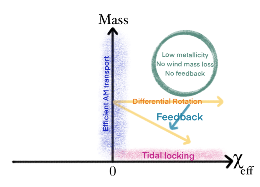
Different models for the evolution of field binaries predict different -mass distribution: There are models that predict all isolated black holes should be born slowly rotating (e.g., Fuller et al., 2019; Fuller & Ma, 2019) and therefore, secondary astrophysical mechanisms such as tidal interactions are invoked to explain fast rotating BHs in either HMXBs or GW151226. Effectively such models predict a distribution of BHs in mass-spin at birth similar to the blue band in Figure 1 for the BBHs.
In the case of moderate efficiency of AM as implemented in MESA stellar evolution model (Eggenberger et al., 2007), low metallicity stars are expected to not lose mass through winds, as their opacity for EUV/UV photons is small (Kudritzki & Puls, 2000; Vink et al., 2001). Therefore, the collapse of such stars is expected to result in both massive, and highly spinning BHs (although in such cases feedback is likely to limit their mass; Batta & Ramirez-Ruiz, 2019). The predicted locus of such objects are depicted by the green circle in Figure 1. Since low metallicity environments are thought to be the underlying requirement for the formation of such BBHs, given the metallicity evolution of the universe, these systems are expected to be likely born at high redshifts (although it is possible to form such systems in pockets of the low metallicity regions in the local universe), and therefore, a long delay time (large separations at birth) are thought to make them merge at such that LIGO can see them. This channel has been proposed to explain GW170729 (Bavera et al., 2019).
Other models with inefficient angular momentum transport can produce a distribution in space with a mean value that decreases and a dispersion that increases with increasing mass (Belczynski et al., 2017), as we find in the GWTC-1 catalog. However, such models generally predict higher values of at low masses than are observed in GWTC-1, and are therefore disfavored (Belczynski et al., 2017). Nevertheless, it may be possible to produce the trends we observe in mean and dispersion with mass through field formation models invoking a combination of efficient angular momentum transport, tidal spin-up, and metallicity-dependent mass loss from high-mass stellar winds that differs from the one explored in Bavera et al. (2019).
Dynamical assembly can also make massive spinning BBH mergers, however, the expected distribution in the case of dynamical assembly is symmetric and therefore future BBH detections can tell us whether there is a locus of BBHs at high mass and high spin, or whether the massive BBHs are symmetrically distributed in . This can shed light on the underlying formation mechanism of such systems and whether their spins have been altered by subsequent stellar encounters (e.g., Lopez et al., 2019).
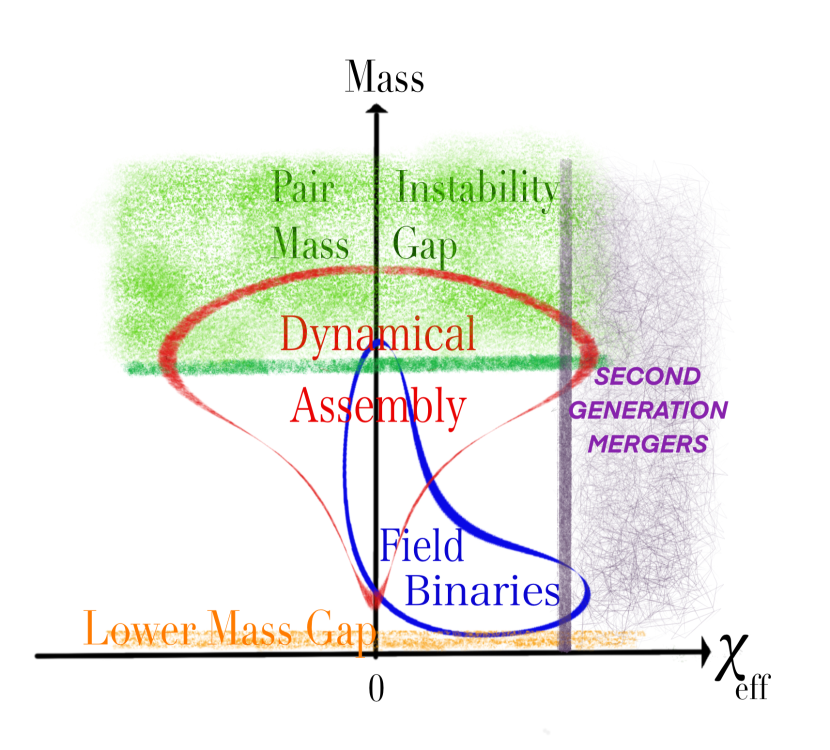
Under dynamical assembly, the predicted -mass distribution is more well defined in its structure: first generation black holes could be born with zero spin, however the final merger product of such black holes will have high spins () (Fishbach et al., 2017; Gerosa & Berti, 2017). The merger of these second generation BHs with either another second generation BHs, or first generation BHs, forms a BBH with at least one of the BHs to be highly spinning. The spin orientation of the BHs in the dynamical assembly would be random with respect to the binary’s orbital plane and therefore the final merger product is expected to show a symmetric distribution around zero that widens at larger masses. The widening at larger masses is due to the merger products of higher generation black holes in a dense cluster like environment (Rodriguez et al., 2019; Doctor et al., 2019).
Figure 2 shows the expected distribution in -mass from two separate categories: Field binaries shown as the blue banana region, and the dynamically assembled binaries shown with red pear like region. These are rough sketches of the expected distributions and not necessarily to scale. The lower orange band indicates the debated lower mass gap (between 2-5 ). The green band and the light green region above it indicates the presence of a drop in mass function of the BBHs given the 10 LIGO/Virgo BBHs (Fishbach & Holz, 2017; Talbot & Thrane, 2018; Roulet & Zaldarriaga, 2019; Safarzadeh & Farr, 2019) due to pulsational pair instability supernovae (Woosley, 2017) where BHs with mass between are expected to not form. The field binaries can provide the negative trend with mass, and the dynamically assembled binaries provide the increase in dispersion with mass, the combination of which can potentially explain our findings.
3 Regression analysis on GWTC-1
In this section we analyze the joint -mass distribution of the ten LIGO/Virgo BBHs to search for possible correlations of the mean and dispersion of the effective spin with mass, where mass can be either the primary mass, the chirp mass, or the total mass of the binary.
We assume that the population distribution for , conditioned on mass, follows
| (3) |
where is a normal distribution with mean , and dispersion . The notation means to truncate the normal distribution to the range . The parameters and are set by the mass of the BBH via
| (4) |
and
| (5) |
Here can be any measure of the mass of the BBHs: the primary mass of the BBH (), the total mass of the system (), or the chirp mass of the system,
| (6) |
where is the symmetric mass ratio given by
| (7) |
We assume a fixed mass and redshift distribution consistent with the population analysis in Abbott et al. (2019a) throughout this work, with
| (8) | |||||
| (9) | |||||
| (10) |
where is the comoving volume (Hogg, 1999). (The redshift distribution gives an observed merger rate that is consistent with the comoving merger rate tracking the low-redshift evolution of the star formation rate (Fishbach et al., 2018; Madau & Dickinson, 2014).) We have verified that our results do not depend on the choice of mass and redshift distribution within the ranges permitted by the population analysis of Abbott et al. (2019a).
The marginal likelihood for the catalog data given population parameters is (Mandel et al., 2018)
| (11) |
where
| (12) |
is the population-averaged detection probability.
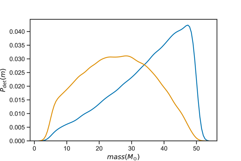
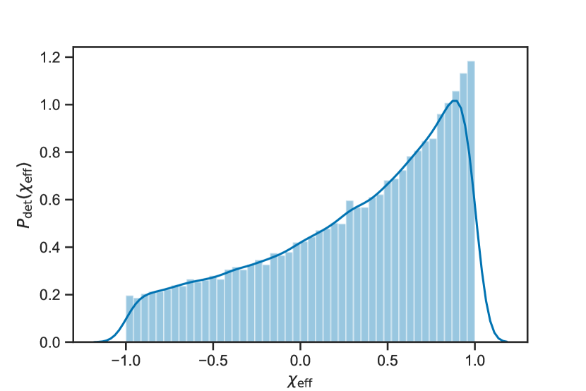
Here we model the detection process semi-analytically, using a method similar to the one described in Abbott et al. (2016), but with a three-detector network (two Advanced LIGO, one Advanced Virgo, all assumed to operate with “early high-sensitivity” noise (Abbott et al., 2018)) and a correspondingly enhanced (noisy) SNR threshold of . For all these calculations we use the IMRPHENOMPV2 waveform family (Hannam et al., 2014). The detection probabilities produced for , , and from our analytic model are shown in Figure 3.
The integral in the product can be approximated as a weighted sum over samples drawn from the likelihood function :
| (13) |
Similarly, can be approximated as a weighted sum over samples drawn from a canonical distribution, , and “detected” by our synthetic pipeline (Farr, 2019):
| (14) |
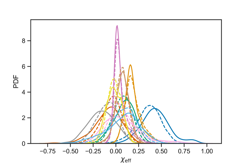
We re-weight the posterior samples of provided by the LVC for each of the BBH systems in GWTC-1 (Abbott et al., 2019b) by the inverse of the LALInference prior (Veitch et al., 2015) to draw samples from the likelihood function. The default prior from LALInference assumes a uniform mass distribution for and in the detector frame, uniform distribution for the magnitude of the spin parameter for each black hole, and uniform prior on the from -1 to 1, and a prior on the luminosity distance proportional to . Figure 4 shows the difference between the posterior samples from the GWTC-1 catalog and the likelihood function for marginalized over our assumed mass and redshift distribution (Eqs. (8), (9), and (10)).
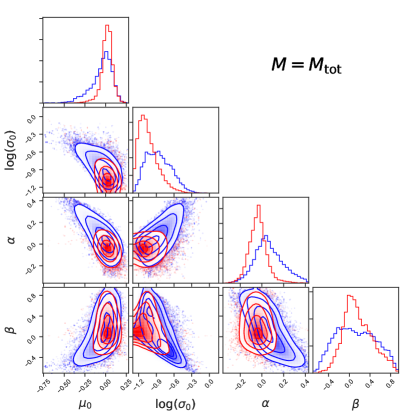
We apply a flat prior on the population parameters , and sample from their posterior distribution given the catalog data (i.e. we draw samples of proportional to the function in Eq. (11)) using the emcee stochastic sampler (Foreman-Mackey et al., 2013) with various choices of mass parameter controlling the distribution. Our results are summarized in Figures 5, 6, and 7.
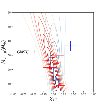
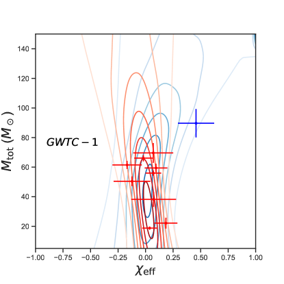
The left panel of Figure 5 shows a contour plot of the posterior distribution in the - plane after analyzing the GWTC-1 BBHs and marginalizing over :
| (15) |
The crosses show the error in chirp mass and of the ten LIGO BBHs. The blue cross represents GW170729 which has the highest observed among the 10 BBH systems. The red contours show the posterior PDF, without considering GW170729, while the blue contours show the result when all of the ten LIGO events are analyzed. We have singled out GW170729 since it has the highest significant false alarm rate (FAR) of 0.18 / year in the GstLAL pipeline (Abbott et al., 2019a) which nearly matches the threshold of 0.1 / year, while the other BBH systems have significantly lower FARs ().
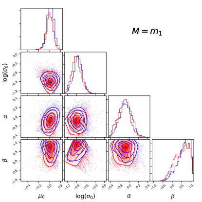
The right panel of Figure 5 shows the posterior PDF of the four parameters in our model used to describe the -mass relation. A negative trend with mass () and a positive trend of dispersion with mass () are favored at 95% and 60% respectively for the case of ignoring GW170729, and 74%, 78% when analyzing all ten LIGO events.
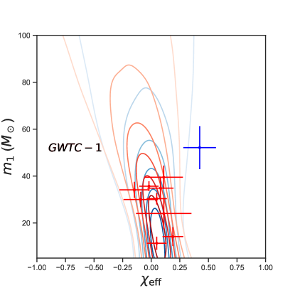
Figure 6 shows the same result but when the mass variable is taken to be the primary mass of the system. When the mass scale is the primary mass of the BBHs, a negative trend with mass () and a positive trend of dispersion with mass () is favored at 80% and 90% respectively for the case of ignoring GW170729, and 70%, 95% in case of analyzing all the ten LIGO events.
Figure 7 shows the same result but when the mass is taken to be the total mass of the system. When the mass scale is the total mass of the BBHs, a negative trend with mass () and a positive trend of dispersion with mass () is favored at 30% and 60% respectively for the case of ignoring GW170729, and 70%, 70% is favored in case of analyzing all the ten LIGO events.
Although the choice of mass scale somewhat affects the confidence by which a trend with mass for either the mean or its dispersion could be detected, the data suggests that if there is a trend, it is a negative trend with mass for the mean and a positive trend for its dispersion. Dynamical assembly alone can account for the larger dispersion in with mass, however the negative trend of the mean with mass can not be accounted for based on dynamical assembly. Field formation of the BBHs on the other hand can potentially explain the negative trend with mass (through a combination of tidally spun up systems at low masses and massive BBHs with about zero effective spin at birth), however, the increase of dispersion with mass would be hard to accommodate based on field evolution alone. Thus we suggest that the observed trends in with mass could be indicating the operation of both formation channels in the GWTC-1 observations.
4 Summary & Conclusion
A given formation channel for a BBH system would predict a certain distribution in -mass plane for the final merger event that LIGO/Virgo would observe. Field binaries tend to predict a banana shaped region that encompass massive systems with negligible magnitude or low mass systems with positive magnitudes if the angular momentum transport is weak. The distribution could be combination of three main mechanism : (i) formation with negligible spin at all masses due to efficient AM transport, (ii) tidal spin of the binaries in which the second born compact object forms from a tidally spun up progenitor in a close orbit with another BH, (iii) formation with moderate efficiency of AM transport while including feedback from disk formation after the core of the progenitor star has collapsed and formed a BH.
On the other hand, dynamical assembly of BBHs in dense stellar clusters leads to a symmetric distribution of BBHs in at all masses with larger dispersion at higher masses. The increase of dispersion is due to a random walk in -mass that higher generation BHs follow.
In this study we find a tentative negative correlation between and chirp mass for the ten LIGO/Virgo BBHs with confidence. The negative correlation could in principle be explained by field formation alone. However, standard field formation consistent with the observed small effective spins at low mass would predict that the dispersion should decrease with mass, the opposite of what the data suggests. We find that the dispersion in grows with mass with 80% confidence. These trends are consistent with a combined channel of dynamically assembled BBHs that provide the positive trend of dispersion with mass, and a field formation channel that provides the negative mean trend with mass could explain our findings.
Given the public alerts released by Advanced LIGO and Virgo111See https://emfollow.docs.ligo.org/userguide/. in the first half of the third observing run, the O3a catalog should contain BBH mergers; therefore, the statistical uncertainties on our parameters should decrease by about a factor of on incorporating the O3a catalog; additional detections in O3b (Abbott et al., 2019b, 2018) should produce a further factor of reduction in uncertainty. Thus we can expect the O3 catalog of BBH systems to confidently confirm or overturn the trends observed here.
References
- Abbott et al. (2016) Abbott, B. P., Abbott, R., Abbott, T. D., et al. 2016, ApJS, 227, 14
- Abbott et al. (2018) —. 2018, Living Reviews in Relativity, 21, 3
- Abbott et al. (2019a) —. 2019a, ApJ, 882, L24
- Abbott et al. (2019b) —. 2019b, Physical Review X, 9, 031040
- Abbott et al . & Collaboration (2016) Abbott et al ., B. P., & Collaboration, t. V. 2016, Physical Review Letters, 688
- Antonini et al. (2017) Antonini, F., Rodriguez, C. L., Petrovich, C., & Fischer, C. L. 2017, Monthly Notices of the Royal Astronomical Society: Letters, L58
- Astropy Collaboration et al. (2013) Astropy Collaboration, Robitaille, T. P., Tollerud, E. J., et al. 2013, A&A, 558, A33
- Batta & Ramirez-Ruiz (2019) Batta, A., & Ramirez-Ruiz, E. 2019, 1904.04835
- Batta et al. (2017) Batta, A., Ramirez-Ruiz, E., & Fryer, C. 2017, ApJ, 846, L15
- Bavera et al. (2019) Bavera, S. S., Fragos, T., Qin, Y., et al. 2019, 1906.12257
- Belczynski et al. (2002) Belczynski, K., Kalogera, V., & Bulik, T. 2002, The Astrophysical Journal, 572, 407
- Belczynski et al. (2017) Belczynski, K., Klencki, J., Fields, C. E., et al. 2017, 1706.07053
- Carpenter et al. (2017) Carpenter, B., Gelman, A., Hoffman, M., et al. 2017, Journal of Statistical Software, Articles, 76, 1
- Chatterjee et al. (2016) Chatterjee, S., Rodriguez, C. L., Kalogera, V., & Rasio, F. A. 2016, The Astrophysical Journal, L26
- Doctor et al. (2019) Doctor, Z., Wysocki, D., O’Shaughnessy, R., Holz, D. E., & Farr, B. 2019, 1911.04424
- Dominik et al. (2012) Dominik, M., Belczynski, K., Fryer, C., et al. 2012, The Astrophysical Journal, 759, 52
- Eggenberger et al. (2007) Eggenberger, P., Meynet, G., Maeder, A., et al. 2007, Astrophysics and Space Science, 316, 43
- Ekström et al. (2011) Ekström, S., Georgy, C., Eggenberger, P., et al. 2011, Astronomy & Astrophysics, A146
- Farr (2019) Farr, W. M. 2019, Research Notes of the American Astronomical Society, 3, 66
- Farr et al. (2017) Farr, W. M., Stevenson, S., Miller, M. C., et al. 2017, Nature, 548, 426
- Fishbach & Holz (2017) Fishbach, M., & Holz, D. E. 2017, The Astrophysical Journal Letters, 851, L25
- Fishbach et al. (2017) Fishbach, M., Holz, D. E., & Farr, B. 2017, ApJ, 840, L24
- Fishbach et al. (2018) Fishbach, M., Holz, D. E., & Farr, W. M. 2018, ApJ, 863, L41
- Foreman-Mackey (2016) Foreman-Mackey, D. 2016, The Journal of Open Source Software, 1, 24
- Foreman-Mackey et al. (2013) Foreman-Mackey, D., Hogg, D. W., Lang, D., & Goodman, J. 2013, Publications of the Astronomical Society of the Pacific, 125, 306
- Fragos & McClintock (2014) Fragos, T., & McClintock, J. E. 2014, ApJ, 17
- Fuller & Ma (2019) Fuller, J., & Ma, L. 2019, The Astrophysical Journal, L1
- Fuller et al. (2019) Fuller, J., Piro, A. L., & Jermyn, A. S. 2019, Monthly Notices of the Royal Astronomical Society, 1902.08227
- Gerosa & Berti (2017) Gerosa, D., & Berti, E. 2017, Phys. Rev. D, 95, 124046
- Gerosa et al. (2018) Gerosa, D., Berti, E., O’Shaughnessy, R., et al. 2018, Physical Review D, 126
- Hannam et al. (2014) Hannam, M., Schmidt, P., Bohé, A., et al. 2014, Phys. Rev. Lett., 113, 151101
- Hogg (1999) Hogg, D. W. 1999, arXiv e-prints, astro
- Hunter (2007) Hunter, J. D. 2007, Computing in Science and Engineering, 9, 90
- Jones et al. (2001–) Jones, E., Oliphant, T., Peterson, P., et al. 2001–, SciPy: Open source scientific tools for Python, [Online; accessed 2019 Aug 23]
- Kudritzki & Puls (2000) Kudritzki, R.-P., & Puls, J. 2000, Annual Review of Astronomy and Astrophysics, 38, 613
- Kumar et al. (2019) Kumar, R., Carroll, C., Hartikainen, A., & Martin, O. A. 2019, The Journal of Open Source Software, doi:10.21105/joss.01143
- Lopez et al. (2019) Lopez, Martin, J., Batta, A., Ramirez-Ruiz, E., Martinez, I., & Samsing, J. 2019, ApJ, 877, 56
- Madau & Dickinson (2014) Madau, P., & Dickinson, M. 2014, Annual Review of Astronomy and Astrophysics, 52, 415
- Mandel et al. (2018) Mandel, I., Farr, W. M., & Gair, J. R. 2018, Monthly Notices of the Royal Astronomical Society, 1086
- Ng et al. (2018) Ng, K. K. Y., Vitale, S., Zimmerman, A., et al. 2018, Phys. Rev. D, 98, 083007
- O’Shaughnessy et al. (2017) O’Shaughnessy, R., Gerosa, D., & Wysocki, D. 2017, Physical Review Letters, 91
- Piran & Piran (2019) Piran, Z., & Piran, T. 2019, arXiv e-prints, arXiv:1910.11358
- Price-Whelan et al. (2018) Price-Whelan, A. M., Sipőcz, B. M., Günther, H. M., et al. 2018, AJ, 156, 123
- Pérez & Granger (2007) Pérez, F., & Granger, B. E. 2007, Computing in Science & Engineering, 9, 21
- Qin et al. (2018) Qin, Y., Marchant, P., Fragos, T., Meynet, G., & Kalogera, V. 2018, The Astrophysical Journal, L18
- Rodriguez et al. (2018) Rodriguez, C. L., Amaro-Seoane, P., Chatterjee, S., et al. 2018, Physical Review D, 1
- Rodriguez & Antonini (2018) Rodriguez, C. L., & Antonini, F. 2018, ApJ, 7
- Rodriguez et al. (2019) Rodriguez, C. L., Zevin, M., Amaro-Seoane, P., et al. 2019, Physical Review D, 043027
- Rodriguez et al. (2016) Rodriguez, C. L., Zevin, M., Pankow, C., Kalogera, V., & Rasio, F. A. 2016, The Astrophysical Journal, L2
- Roulet & Zaldarriaga (2019) Roulet, J., & Zaldarriaga, M. 2019, Monthly Notices of the Royal Astronomical Society, 484, 4216
- Safarzadeh & Farr (2019) Safarzadeh, M., & Farr, W. M. 2019, The Astrophysical Journal, L24
- Safarzadeh et al. (2019) Safarzadeh, M., Hamers, A. S., Loeb, A., & Berger, E. 2019, arXiv e-prints, arXiv:1911.04495
- Samsing et al. (2014) Samsing, J., MacLeod, M., & Ramirez-Ruiz, E. 2014, ApJ, 784, 71
- Samsing et al. (2018) —. 2018, ApJ, 853, 140
- Schrøder et al. (2018) Schrøder, S. L., Batta, A., & Ramirez-Ruiz, E. 2018, ApJ, 862, L3
- Spruit (1999) Spruit, H. C. 1999
- Spruit (2001) —. 2001, Astronomy & Astrophysics, 381, 923
- Stan Development Team (2018) Stan Development Team. 2018, PyStan: The Python Interface to Stan
- Stevenson et al. (2017) Stevenson, S., Berry, C. P. L., & Mandel, I. 2017, MNRAS, 471, 2801
- Talbot & Thrane (2018) Talbot, C., & Thrane, E. 2018, The Astrophysical Journal, 856, 173
- Veitch et al. (2015) Veitch, J., Raymond, V., Farr, B., et al. 2015, Phys. Rev. D, 91, 042003
- Venumadhav et al. (2019a) Venumadhav, T., Zackay, B., Roulet, J., Dai, L., & Zaldarriaga, M. 2019a, arXiv e-prints, arXiv:1904.07214
- Venumadhav et al. (2019b) —. 2019b, Phys. Rev. D, 100, 023011
- Vink et al. (2001) Vink, J. S., de Koter, A., & Lamers, H. J. G. L. M. 2001, Astronomy & Astrophysics, 369, 574
- Vitale et al. (2017a) Vitale, S., Gerosa, D., Haster, C.-J., Chatziioannou, K., & Zimmerman, A. 2017a, Phys. Rev. Lett., 119, 251103
- Vitale et al. (2017b) Vitale, S., Lynch, R., Sturani, R., & Graff, P. 2017b, Classical and Quantum Gravity, 34, 03LT01
- Walt et al. (2011) Walt, S. v. d., Colbert, S. C., & Varoquaux, G. 2011, Computing in Science & Engineering, 13, 22
- Waskom et al. (2018) Waskom, M., Botvinnik, O., O’Kane, D., et al. 2018, mwaskom/seaborn: v0.9.0 (July 2018), doi:10.5281/zenodo.1313201
- Woosley (2017) Woosley, S. E. 2017, The Astrophysical Journal, 836, 244
- Zackay et al. (2019) Zackay, B., Venumadhav, T., Dai, L., Roulet, J., & Zaldarriaga, M. 2019, Phys. Rev. D, 100, 023007
- Zaldarriaga et al. (2017a) Zaldarriaga, M., Kushnir, D., & Kollmeier, J. A. 2017a, Monthly Notices of the Royal Astronomical Society, 4174
- Zaldarriaga et al. (2017b) —. 2017b, Monthly Notices of the Royal Astronomical Society, 473, 4174
- Zwart et al. (2004) Zwart, S. P., Baumgardt, H., Hut, P., Makino, J., & McMillan, S. 2004, Nature, 428, 724