On Covering Numbers, Young Diagrams, and the Local Dimension of Posets

Abstract

We study covering numbers and local covering numbers with respect to difference graphs and complete bipartite graphs. In particular we show that in every cover of a Young diagram with $\binom{2k}{k}$ steps with generalized rectangles there is a row or a column in the diagram that is used by at least $k+1$ rectangles, and prove that this is best-possible. This answers two questions by Kim, Martin, Masařík, Shull, Smith, Uzzell, and Wang [15], namely:

1. What is the local complete bipartite cover number of a difference graph?

2. Is there a sequence of graphs with constant local difference graph cover number and unbounded local complete bipartite cover number?

We add to the study of these local covering numbers with a lower bound construction and some examples. Following Kim et al., we use the results on local covering numbers to provide lower and upper bounds for the local dimension of partially ordered sets of height 2. We discuss the local dimension of some posets related to Boolean lattices and show that the poset induced by the first two layers of the Boolean lattice has local dimension $(1+o(1))\log_{2}\log_{2}n$. We conclude with some remarks on covering numbers for digraphs and Ferrers dimension.

1 Introduction

The covering number of a graph $H$ (host) with respect to a class $\mathfrak{F}$ is the least $k$ such that there are graphs $G_{1},\ldots,G_{k}\in\mathfrak{F}$ with $G_{i}\subset H$ for $i\in[k]$ such that their union covers the edges of $H$ and no other edges. We denote this number by $\operatorname{c}^{\mathfrak{F}}(H)$. The study of covering numbers has a long tradition:

• In 1891 Petersen [20] showed that the covering number of $2k$-regular graphs with respect to $2$-regular graphs is $k$.

• In 1964 Nash-William [19] defined the arboricity of a graph as the covering number respect to forests and showed that it equals the lower bound given by the maximum local density.

• The track number introduced by Gyárfás and West [11] and the thickness introduced by Aggarwal et al. [1] correspond to covering numbers with respect to interval graphs and planar graphs respectively.

Knauer and Ueckerdt [17] proposed the study of local covering numbers. This number is defined as the minimum number $k$ such that there is a cover of $H$ with graphs from $\mathfrak{F}$ (see above) such that every vertex of $H$ is contained in at most $k$ members of the cover. We denote the local covering number by $\operatorname{c}_{\ell}^{\mathfrak{F}}(H)$. Fishburn and Hammer [9] introduced the bipartite degree which equals what we call the local covering number with respect to complete bipartite graphs. Motivated by questions regarding the local dimension of posets, Kim et al. [15] studied local covering number with respect to difference graphs and compare this to the local covering number with respect to complete bipartite graphs.

In this paper we continue the studies initiated in [15]. In Section 2 we discuss local coverings with difference graphs and complete bipartite graphs. With Theorem 1 we give a precise result regarding the local covering number of a difference graph (Young diagram) with respect to complete bipartite graphs (generalized rectangles). This answers a question raised in [15].

Section 3 relates the results to the local dimension of posets. In this section we also discuss aspects of the local dimension of Boolean lattices. Finally, in Section 4 we discuss covering numbers of directed graphs and their relation with order dimension and notions of Ferrers dimension.

2 Covering numbers

Following the notation in [17], local covering numbers are defined as follows. For a graph class $\mathfrak{F}$ and a graph $H$, an $\mathfrak{F}$-covering of $H$ is a set of graphs $G_{1},\ldots,G_{t}\in\mathfrak{F}$ with $H=G_{1}\cup\cdots\cup G_{t}$. (In [17] this is called an injective $\mathfrak{F}$-covering. But as all coverings considered here are injective, we omit this specification throughout.) An $\mathfrak{F}$-covering of $H$ is $k$-local if every vertex of $H$ is contained in at most $k$ of the graphs $G_{1},\ldots,G_{t}$, and the local $\mathfrak{F}$-covering number of $H$, denoted by $\operatorname{c}_{\ell}^{\mathfrak{F}}(H)$, is the smallest $k$ for which a $k$-local $\mathfrak{F}$-cover of $H$ exists.

A difference graph is a bipartite graph in which the vertices of one partite set can be ordered $a_{1},\ldots,a_{r}$ in such a way that $N(a_{i})\subseteq N(a_{i-1})$ for $i=2,\ldots,r$, i.e., the neighbourhoods of these vertices along this ordering are weakly nesting.

Difference graphs are closely related to Young diagrams. Let $\mathbb{N}$ denote the set of positive integers. For $x\in\mathbb{N}$ we denote $[x]=\{1,\ldots,x\}$. A Young diagram with $r$ rows and $c$ columns is a subset $Y\subseteq[r]\times[c]$ such that whenever $(i,j)\in Y$, then $(i-1,j)\in Y$ provided $i\geq 2$, as well as $(i,j-1)\in Y$ provided $j\geq 2$. A Young diagram is visualized as a set of axis-aligned unit squares, called cells that are arranged consecutively in rows and columns, each row starting in the first column, and with every row (except the first) being at most as long as the row above.

A generalized rectangle (also called combinatorial rectangle) in a Young diagram $Y\subseteq[r]\times[c]$ is a set $R$ of the form $R=S\times T$ with $S\subseteq[r]$ and $T\subseteq[c]$ and $R\subseteq Y$. Note that (unless $Y=[r]\times[c]$) not every set of the form $R=S\times T$ with $S\subseteq[r]$ and $T\subseteq[c]$ satisfies $R\subseteq Y$. A generalized rectangle $R=S\times T$ with $S$ being a set of consecutive numbers in $[r]$ and $T$ being a set of consecutive numbers in $[c]$ is an actual rectangle. A generalized rectangle $R=S\times T$ uses the rows in $S$ and the columns in $T$. See Figure 2 for an illustrative example.

Difference graphs can be characterized as those bipartite graphs $H=(V,E)$ with bipartition $V=A\mathop{\mathbin{\mathchoice{\leavevmode\vtop{\halign{\hfil$\m@th\displaystyle#$\hfil\cr\cup\cr\cdot\crcr}}}{\leavevmode\vtop{\halign{\hfil$\m@th\textstyle#$\hfil\cr\cup\cr\cdot\crcr}}}{\leavevmode\vtop{\halign{\hfil$\m@th\scriptstyle#$\hfil\cr\cup\cr\cdot\crcr}}}{\leavevmode\vtop{\halign{\hfil$\m@th\scriptscriptstyle#$\hfil\cr\cup\cr\cdot\crcr}}}}}B$, $|A|=r,|B|=c$, which admit a bipartite adjacency matrix $M=(m_{s,t})_{s\in A,t\in B}$ whose support is a Young diagram $Y\subseteq[r]\times[c]$:

$$\forall s\in A,t\in B\colon\qquad\{s,t\}\in E\quad\Leftrightarrow\quad(s,t)\in Y\quad\Leftrightarrow\quad m_{s,t}=1$$

Moreover, a complete bipartite subgraph $G$ of $H$ corresponds to a generalized rectangle $R$ in $Y$. Rows and columns of $M$ correspond to vertices of $H$ in $A$ and $B$, respectively.

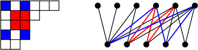
Figure 1: Left: A Young diagram $Y$ with $r=5$ rows and $c=6$ columns. Highlighted are the generalized rectangle $\{1,4\}\times\{1,3\}$ (blue), and the actual rectangle $\{2,3\}\times\{2,3\}$ (red). Right: A corresponding difference graph with corresponding red and blue $K_{2,2}$.

In [15], Kim et al. introduced the concept of covering a Young diagram with generalized rectangles subject to minimizing the maximum number of rectangles intersecting any row or column. Their motivation was to investigate the relations between local difference cover numbers and local complete bipartite cover numbers.

Let $\mathfrak{D}$ denote the class of all difference graphs, and ${\mathfrak{C}\mathfrak{B}}\subset\mathfrak{D}$ the class of all complete bipartite graphs. Clearly, we have $\operatorname{c}_{\ell}^{\mathfrak{D}}(H)\leq\operatorname{c}_{\ell}^{{\mathfrak{C}\mathfrak{B}}}(H)$ for all graphs $H$. Kim et al. [15] asked whether there is a sequence of graphs $(H_{i}\colon i\in\mathbb{N})$ for which $\operatorname{c}_{\ell}^{\mathfrak{D}}(H_{i})$ is constant while $\operatorname{c}_{\ell}^{{\mathfrak{C}\mathfrak{B}}}(H_{i})$ is unbounded. They prove that for all graphs $H$ on $n$ vertices,

$$\operatorname{c}_{\ell}^{{\mathfrak{C}\mathfrak{B}}}(H)\leq\operatorname{c}_{\ell}^{\mathfrak{D}}(H)\cdot\left\lceil\log_{2}(n/2+1)\right\rceil,$$

by showing that $\operatorname{c}_{\ell}^{{\mathfrak{C}\mathfrak{B}}}(H)\leq\lceil\log_{2}(r+1)\rceil$ whenever $H\in\mathfrak{D}$ is a difference graph with one partite set of size $r$. However, no lower bound on $\operatorname{c}_{\ell}^{{\mathfrak{C}\mathfrak{B}}}(H)$ for $H\in\mathfrak{D}$ is established in [15]. Specifically, Kim et al. ask for the exact value of $\operatorname{c}_{\ell}^{{\mathfrak{C}\mathfrak{B}}}(H_{i})$ for the difference graph $H_{i}$ with vertex set $\{a_{1},\ldots,a_{i}\}\cup\{b_{1},\ldots,b_{i}\}$ and $N(a_{j})=\{b_{1},\ldots,b_{j}\}$ for all $j\in[i]$. For the case that $i+1$ is a power of $2$ they prove the upper bound $\operatorname{c}_{\ell}^{{\mathfrak{C}\mathfrak{B}}}(H_{i})\leq\log_{2}(i+1)-1$.

The number of steps of a Young diagram $Y\subseteq[r]\times[c]$ is the number of different row lengths in $Y$, i.e., the cardinality of

$$Z=\{(s,t)\in Y\mid(s+1,t)\notin Y\text{ and }(s,t+1)\notin Y\}.$$

The cells in $Z$ are called the steps of $Y$. Young diagrams with $n$ elements, $r$ rows, $c$ columns, and $z$ steps, visualize partitions of $n$ into $r$ unlabeled summands (row lengths) with summands of $z$ different values and largest summand being $c$.

We say that $Y$ is covered by a set $C$ of generalized rectangles if $Y=\bigcup_{R\in C}R$, i.e., $Y$ is the union of all rectangles in $C$. In this case we also say that $C$ is a cover of $Y$. If additionally the rectangles in $C$ are pairwise disjoint, we call $C$ a partition of $Y$. For example, Figure 2 shows a Young diagram with a partition into actual rectangles.

Theorem 1.

For any $k\in\mathbb{N}$, any Young diagram $Y$ can be covered by a set $C$ of generalized rectangles such that each row and each column of $Y$ is used by at most $k$ rectangles in $C$ if and only if $Y$ has strictly less than $\binom{2k}{k}$ steps.

The Young diagram of the difference graph $H_{i}$ is $Y_{i}=\{(s,t)\in[i]\times[i]\mid s+t\leq i+1\}$, i.e., the (unique) Young diagram with $i$ rows, $i$ columns, and $i$ steps. Therefore Theorem 1 answers the questions raised by Kim et al..

2.1 Proof of Theorem 1

Throughout we shall simply use the term rectangle for generalized rectangles, and rely on the term actual rectangle when specifically meaning rectangles that are contiguous. For a Young diagram $Y$ and $i,j\in\mathbb{N}$, let us define a cover $C$ of $Y$ to be $(i,j)$-local if each row of $Y$ is used by at most $i$ rectangles in $C$ and each column of $Y$ is used by at most $j$ rectangles in $C$. Recall that $Y_{z}$ is the Young diagram with $z$ rows, $z$ columns, and $z$ steps. See Figure 2.

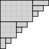
Figure 2: The Young diagram $Y_{9}$ with $9$ steps and a $(2,3)$-local partition of $Y$ with actual rectangles.

We start with a lemma stating that instead of considering any Young diagram with $z$ steps, we may restrict our attention to just $Y_{z}$.

Lemma 2.

Let $i,j,z\in\mathbb{N}$ and $Y$ be any Young diagram with $z$ steps. Then $Y$ admits an $(i,j)$-local cover if and only if $Y_{z}$ admits an $(i,j)$-local cover with exactly $z$ rectangles.

Proof.

First assume that $Y$ admits an $(i,j)$-local cover $C$. If $C$ consists of strictly more than $z$ rectangles, as every rectangle is contained in a $[s]\times[t]$ for some step $(s,t)\in Z$, by the pigeonhole principle there are $R_{1},R_{2}\in C$, $R_{1}\neq R_{2}$, such that $R_{1},R_{2}\subseteq[s]\times[t]$ for some step $(s,t)\in Z$. However, in this case $C-\{R_{1},R_{2}\}+\{R_{1}\cup R_{2}\}$ is also an $(i,j)$-local cover of $Y$ with one rectangle less, where $\{R_{1}\cup R_{2}\}$ denotes the rectangle whose row set and column set is the union of the row set and column set of $R_{1}$ and $R_{2}$. Thus, by repeating this argument, we may assume that $|C|=z$.

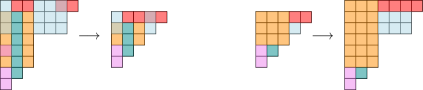
Figure 3: Transforming a cover of any Young diagram $Y$ with $5$ steps into a cover of $Y_{5}$ (left) and vice versa (right).

If $Y\neq Y_{z}$, there is a row $s$ or a column $t$ that is not used by any step in $Z$. Apply the mapping $\mathbb{N}\times\mathbb{N}\to\mathbb{N}\times\mathbb{N}$ with

$$(x,y)\mapsto\begin{cases}(x,y)&\text{ if }x<s\\ (x-1,y)&\text{ if }x\geq s\end{cases} (x,y)\mapsto\begin{cases}(x,y)&\text{ if }y<t\\ (x,y-1)&\text{ if }y\geq t\end{cases}$$ respectively

Intuitively, we cut out row $s$ (respectively column $t$), moving all rows below one step up (respectively all columns to the right one step left). This gives an $(i,j)$-local cover of a smaller Young diagram with $z$ steps, and eventually leads to an $(i,j)$-local cover of $Y_{z}$, as desired. See the left of Figure 3.

On the other hand, if $Y_{z}$ admits an $(i,j)$-local cover $C=\{R_{1},\ldots,R_{z}\}$, this defines an $(i,j)$-local cover of $Y$ as follows. Index the rows used by the steps $Z$ of $Y$ by $s_{1}<\cdots<s_{z}$ and the columns used by the steps $Z$ of $Y$ by $t_{1}<\cdots<t_{z}$ and let $s_{0}=t_{0}=0$. Defining

$$R^{\prime}_{a}=\{(s,t)\in Y\mid s_{x-1}<s\leq s_{x}\text{ and }t_{y-1}<t\leq t_{y}\text{ for some }(x,y)\in R_{a}\}$$

for $a=1,\ldots,z$ gives an $(i,j)$-local cover $\{R^{\prime}_{1},\ldots,R^{\prime}_{z}\}$ of $Y$. See the right of Figure 3.

Observe that the construction maps an actual rectangle $R_{a}$ of $Y_{z}$ to an actual rectangle $R^{\prime}_{a}$ of $Y$. Also, if $\{R_{1},\ldots,R_{z}\}$ is a partition of $Y_{z}$, then $\{R^{\prime}_{1},\ldots,R^{\prime}_{z}\}$ is a partition of $Y$. This will be used in the proof of Item (i) of Theorem 3. ∎

Let us now turn to our main result. In fact, we shall prove the following strengthening of Theorem 1.

Theorem 3.

For any $i,j,z\in\mathbb{N}$ and any Young diagram $Y$ with $z$ steps, the following hold.

1. If $z<\binom{i+j}{i}$, then there exists an $(i,j)$-local partition of $Y$ with actual rectangles.

2. If $z\geq\binom{i+j}{i}$, then there exists no $(i,j)$-local cover of $Y$ with generalized rectangles.

Proof.

First, let us prove Item (i). For shorthand notation, we define $f(i,j):=\binom{i+j}{i}-1$. It will be crucial for us that the numbers $\{f(i,j)\}_{i,j\geq 1}$ solve the recursion

$$f(i,j)=\begin{cases}f(i-1,j)+f(i,j-1)+1&\text{ if }i,j\geq 2\\ j&\text{ if }i=1,j\geq 1\\ i&\text{ if }i\geq 1,j=1.\end{cases}$$ (1)

This follows directly from Pascal’s rule $\binom{a}{b}=\binom{a-1}{b-1}+\binom{a-1}{b}$ for any $a,b\in\mathbb{N}$ with $1\leq b\leq a-1$.

Due to Lemma 2 it suffices to show that for any $i,j\in\mathbb{N}$ and $z=f(i,j)=\binom{i+j}{i}-1$, there is an $(i,j)$-local partition of $Y_{z}$ with actual rectangles.

We define the $(i,j)$-local partition $C$ by induction on $i$ and $j$. For illustrations refer to Figure 4.

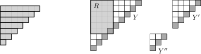
Figure 4: Left: The Young diagram $Y_{z}$ with $z=f(1,7)=\binom{1+7}{1}-1=7$ steps and a $(1,7)$-local partition of $Y_{z}$ into actual rectangles. Right: The Young diagram $Y_{z}$ with $z=f(3,2)=\binom{3+2}{3}-1=9$ steps, the rectangle $R=[a]\times[z+1-a]=[6]\times[4]$ with $a=f(2,2)+1=6$, and the Young diagrams $Y^{\prime}$ and $Y^{\prime\prime}$ with $f(2,2)=5$ and $f(3,1)=3$ steps, respectively.

If $i=1$, respectively $j=1$, then $C$ is the set of rows of $Y_{j}$, respectively the set of columns of $Y_{i}$. If $i\geq 2$ and $j\geq 2$, then $z=f(i,j)=f(i-1,j)+f(i,j-1)+1$ by (1). Consider the actual rectangle $R=[a]\times[z+1-a]$ for $a=f(i-1,j)+1$. Then $Y_{z}-R$ splits into a right-shifted copy $Y^{\prime}$ of $Y_{a-1}$ and a down-shifted copy $Y^{\prime\prime}$ of $Y_{z-a}$. Note that $a-1=f(i-1,j)$ and $z-a=f(i,j-1)$.

By induction we have an $(i-1,j)$-local cover $C^{\prime}$ of $Y^{\prime}$ and an $(i,j-1)$-local cover $C^{\prime\prime}$ of $Y^{\prime\prime}$, each consisting of pairwise disjoint actual rectangles. Define

$$C=\{R\}\cup C^{\prime}\cup C^{\prime\prime},$$

this is a cover of $Y_{z}$ consisting of pairwise disjoint actual rectangles. Rows $1$ to $a$ are used by $R$ and at most $i-1$ rectangles in $C^{\prime}$, and rows $a+1$ to $z$ are used by at most $i$ rectangles in $C^{\prime\prime}$. Hence each row of $Y_{z}$ is used by at most $i$ rectangles in $C$. Similarly each column of $Y_{z}$ is used by at most $j$ rectangles in $C$. Thus $C$ is an $(i,j)$-local partition of $Y_{z}$ by actual rectangles, as desired.

For $z^{\prime}<z=f(i,j)$ we obtain an $(i,j)$-local partition of $Y_{z^{\prime}}$ by restricting the rectangles of the cover $C$ of $Y_{z}$ to the rows from $z-z^{\prime}$ to $z$. This yields an $(i,j)$-local partition of a down-shifted copy $Y^{\prime}$ of $Y_{z^{\prime}}$.

Now, let us prove Item (ii). Due to Lemma 2 it is sufficient to show that for $i,j\in\mathbb{N}$ the Young diagram $Y_{z^{\prime}}$ with $z^{\prime}\geq\binom{i+j}{i}$ admits no $(i,j)$-local cover. If $Y_{z^{\prime}}$ with $z^{\prime}>z=\binom{i+j}{i}$ has an $(i,j)$-local cover, then by restricting the rectangles of the cover to the rows from $z^{\prime}-z$ to $z^{\prime}$ we obtain an $(i,j)$-local cover of a down-shifted copy of $Y_{z}$. Therefore, we only have to consider $Y_{z}$.

Let $C$ be a cover of $Y_{z}$. We shall prove that $C$ is not $(i,j)$-local. Again, we proceed by induction on $i$ and $j$, where illustrations are given in Figure 5.

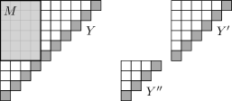
Figure 5: The Young diagram $Y_{z}$ with $z=\binom{3+2}{3}=10$ steps, the rectangle $M=[a]\times[z-a]=[6]\times[4]$ with $a=\binom{2+2}{2}=6$, and the Young diagrams $Y^{\prime}$ and $Y^{\prime\prime}$ with $\binom{2+2}{2}=6$ and $\binom{3+1}{3}=4$ steps, respectively.

If $i=1$, then each row is only used by a single rectangle in $C$, otherwise, $C$ would not be $(1,j)$-local. Hence, each row of $Y_{z}$ is a rectangle in $C$. Thus column $1$ of $Y_{z}$ is used by $z=j+1$ rectangles, proving that $C$ is not $(i,j)$-local.

The case $j=1$ is symmetric to the previous by exchanging rows and columns.

Now let $i\geq 2$ and $j\geq 2$. We have $z=\binom{i+j}{i}=\binom{(i-1)+j}{i-1}+\binom{i+(j-1)}{i}$. Consider the rectangle $M=[a]\times[z-a]$ for $a=\binom{(i-1)+j}{i-1}$. Then $Y_{z}-M$ splits into a right-shifted $Y^{\prime}$ copy of $Y_{a}$ and a down-shifted copy $Y^{\prime\prime}$ of $Y_{z-a}$. Note that $z-a=\binom{i+(j-1)}{i}$.

Let $C^{\prime}$, respectively $C^{\prime\prime}$, be the subset of rectangles in $C$ using at least one of the rows $1,\ldots,a$ in $Y^{\prime}$, respectively at least one of the columns $1,\ldots,z-a$ in $Y^{\prime\prime}$. Note that $C^{\prime}\cap C^{\prime\prime}=\emptyset$ as each generalized rectangle is contained in $Y_{z}$.

Prune each rectangle in $C^{\prime}$ to the columns $z-a+1,\ldots,z$ and each rectangle in $C^{\prime\prime}$ to the rows $a+1,\ldots,z$. This yields covers of $Y^{\prime}$ and $Y^{\prime\prime}$.

The Young diagram $Y^{\prime}$ is a copy of $Y_{a}$ and $a=\binom{(i-1)+j}{i-1}$. Hence, by induction the pruned cover $C^{\prime}$ is not $(i-1,j)$-local. If some column $t$ of $Y^{\prime}$ is used by at least $j+1$ rectangles in $C^{\prime}$, this column of $Y_{z}$ is used by at least $j+1$ rectangles in $C$, proving that $C$ is not $(i,j)$-local, as desired. So we may assume that some row $s$ of $Y^{\prime}$ is used by at least $i$ rectangles in $C^{\prime}$.

Symmetrically, $Y^{\prime\prime}$ is a copy of $Y_{z-a}$ and $z-a=\binom{i+(j-1)}{i}$. Hence, the pruned $C^{\prime\prime}$ is a cover of $Y^{\prime\prime}$, which by induction is not $(i,j-1)$-local, and we may assume that some column $t$ of $Y^{\prime\prime}$ is used by at least $j$ rectangles in $C^{\prime\prime}$. Hence row $s$ in $Y_{z}$ is used by at least $i$ rectangles in $C^{\prime}$ and column $t$ in $Y_{z}$ is used by at least $j$ rectangles in $C^{\prime\prime}$. As $C^{\prime}\cap C^{\prime\prime}=\emptyset$ and element $(s,t)$ is contained in some rectangle of $C$, either row $s$ of $Y_{z}$ is used by at least $i+1$ rectangles or column $t$ of $Y_{z}$ is used by at least $j+1$ rectangles (or both), proving that $C$ is not $(i,j)$-local. ∎

Finally, Theorem 1 follows from Theorem 3 by setting $i=j=k$.

2.2 More about local covering numbers

Using Theorem 1 and $\binom{2k}{k}=(1+o(1))\frac{1}{\sqrt{k\pi}}2^{2k}$, we see that

• for every difference graph $H$ the exact value of $\operatorname{c}_{\ell}^{{\mathfrak{C}\mathfrak{B}}}(H)$ is the smallest $k\in\mathbb{N}$ such that for the number $z$ of steps of $H$ it holds that $z<\binom{2k}{k}$,

• the difference graphs $H_{i}$, $i\in\mathbb{N}$ (corresponding to the Young diagrams $Y_{i}$, $i\in\mathbb{N}$), defined by Kim et al. satisfy

  $$\operatorname{c}_{\ell}^{{\mathfrak{C}\mathfrak{B}}}(H_{i})=\tfrac{1}{2}\log_{2}i+\tfrac{1}{4}\log_{2}\log_{2}i+O(1),$$

  (and, using more precise bounds on Stirling’s approximation, it can be shown that the $O(1)$ term is at most $2$ for all $i\geq 2$),

• for this sequence $(H_{i}\colon i\in\mathbb{N})$ of difference graphs $\operatorname{c}_{\ell}^{\mathfrak{D}}(H_{i})$ is constant $1$, while $\operatorname{c}_{\ell}^{{\mathfrak{C}\mathfrak{B}}}(H_{i})$ is unbounded, and

• for all graphs $H$ on $n$ vertices,

  $$\operatorname{c}_{\ell}^{{\mathfrak{C}\mathfrak{B}}}(H)\leq\operatorname{c}_{\ell}^{\mathfrak{D}}(H)\cdot\left(\tfrac{1}{2}\log_{2}\tfrac{n}{2}+\tfrac{1}{4}\log_{2}\log_{2}\tfrac{n}{2}+2\right).$$

It is also interesting to understand the worst case scenario in covering a bipartite graph by complete bipartite graphs or difference graphs. With a different proof, the following result was already shown in [15].

Theorem 4.

For any $n$ there exists a bipartite graph $H$ on $n$ vertices such that $\operatorname{c}_{\ell}^{\mathfrak{D}}(H)=\Omega(n/\log n)$.

Proof.

Suppose $n\geq 2$ is even. Consider a random bipartite graph $G$ with vertex classes $A$ and $B$, where $|A|=|B|=n/2$ and each edge is chosen with probability $1/2$. For any $t\geq 2$, the expected number of $K_{t,t}$’s in $G$ is $2^{-t^{2}}\binom{n/2}{t}^{2}<2^{-t^{2}}\left(n/2\right)^{2t}$. If we choose $t=\lceil 2\log_{2}n\rceil$, then the expected number of $K_{t,t}$’s (and hence the probability that $G$ contains a $K_{t,t}$) is less than $1/2$. The probability that $e(G)\geq\frac{1}{8}n^{2}$ is at least $1/2$, so with nonzero probability $e(G)\geq\frac{1}{8}n^{2}$ and $G$ has no $K_{t,t}$.

Now consider a cover of $G$ with difference graphs. We call a star an $A$-star (resp. $B$-star) if its centre is in $A$ (resp. $B$). No difference graph in the cover contains a $K_{t,t}$ and thus every difference graph in the cover can be decomposed into at most $t-1$ $A$-stars and at most $t-1$ $B$-stars. Without loss of generality, at least half the edges of $G$ are covered by $A$-stars. As $B$ has $n/2$ vertices, among the $\frac{1}{16}n^{2}$ edges covered by $A$-stars there are at least $n/8$ incident to some vertex $v\in B$. Each difference graph in the cover contributes at most $t-1\leq 2\log_{2}n$ of the $A$-stars containing $v$. Therefore at least $\frac{n}{16\log_{2}n}$ difference graphs of the cover contain $v$. ∎

As Kim et al. [15] already observed, the upper bound follows from a theorem of Erdős and Pyber [7], which shows that a cover of corresponding size exists even with complete bipartite graphs.

Theorem 5 (Erdős and Pyber).

For any simple graph $H$ on $n$ vertices, $\operatorname{c}_{\ell}^{{\mathfrak{C}\mathfrak{B}}}(H)=O(n/\log n)$.

Hansel [12] (see also Király, Nagy, Pálvölgyi and Visontai [16] and Bollobás and Scott [3]) proved that $\operatorname{c}_{\ell}^{{\mathfrak{C}\mathfrak{B}}}(K_{n})\geq\log_{2}n$, which together with the obvious upper bound gives the following proposition:

Proposition 6.

For all $n$, $\operatorname{c}_{\ell}^{{\mathfrak{C}\mathfrak{B}}}(K_{n})=\lceil\log_{2}n\rceil$.

In fact, Hansel proved a somewhat stronger result, namely that, for every ${\mathfrak{C}\mathfrak{B}}$-covering of $K_{n}$, the average number of complete bipartite graphs in which a vertex appears is at least $\log_{2}n$.

An interesting case is $K^{\star}_{n,n}$, which is obtained by deleting the edges of a perfect matching from the complete bipartite graph $K_{n,n}$. Note that $K^{\star}_{n,n}$ is the union of two difference graphs. What is the best covering of this graph by complete bipartite graphs?

Proposition 7.

$\operatorname{c}_{\ell}^{{\mathfrak{C}\mathfrak{B}}}(K^{\star}_{n,n})\leq\operatorname{c}_{\ell}^{{\mathfrak{C}\mathfrak{B}}}(K_{n})\leq 2\operatorname{c}_{\ell}^{{\mathfrak{C}\mathfrak{B}}}(K^{\star}_{n,n})$ and therefore $\operatorname{c}_{\ell}^{{\mathfrak{C}\mathfrak{B}}}(K^{\star}_{n,n})=\Theta(\log n)$.

Proof.

Let us denote the vertices of $K_{n}$ by $\{v_{1},v_{2},\dots v_{n}\}$, and the vertices of $K^{\star}_{n,n}$ by $\{a_{1},a_{2},\dots a_{n},b_{1},b_{2},\dots b_{n}\}$ where $a_{i}b_{j}\in E(K^{\star}_{n,n})\Leftrightarrow i\not=j$. One can easily obtain a covering of $K^{\star}_{n,n}$ from a covering of $K_{n}$. For every complete bipartite graph in the covering with vertex classes $\{v_{i_{1}},v_{i_{2}},\dots v_{i_{p}}\}$ and $\{v_{j_{1}},v_{j_{2}},\dots v_{j_{q}}\}$ take the complete bipartite graph with vertex classes $\{a_{i_{1}},a_{i_{2}},\dots a_{i_{p}}\}$ and $\{b_{j_{1}},b_{j_{2}},\dots b_{j_{q}}\}$ and another one with vertex classes $\{b_{i_{1}},b_{i_{2}},\dots b_{i_{p}}\}$ and $\{a_{j_{1}},a_{j_{2}},\dots a_{j_{q}}\}$. This will be a covering of $K^{\star}_{n,n}$ where the vertices $a_{i}$ and $b_{i}$ are covered exactly as many times as $v_{i}$ in the covering of $K_{n}$. This construction shows $\operatorname{c}_{\ell}^{{\mathfrak{C}\mathfrak{B}}}(K^{\star}_{n,n})\leq\operatorname{c}_{\ell}^{{\mathfrak{C}\mathfrak{B}}}(K_{n})$.

On the other hand, we can obtain a covering of $K_{n}$ from a covering of $K^{\star}_{n,n}$. For a complete bipartite graph in the covering with vertex classes $\{a_{i_{1}},a_{i_{2}},\dots a_{i_{p}}\}$ and $\{b_{j_{1}},b_{j_{2}},\dots b_{j_{q}}\}$ take the complete bipartite graph with vertex classes $\{v_{i_{1}},v_{i_{2}},\dots v_{i_{p}}\}$ and $\{v_{j_{1}},v_{j_{2}},\dots v_{j_{q}}\}$. This will be a covering of $K_{n}$ where the vertex $v_{i}$ is covered exactly as many times as $a_{i}$ and $b_{i}$ are covered in total in the covering of $K^{\star}_{n,n}$. This construction shows $\operatorname{c}_{\ell}^{{\mathfrak{C}\mathfrak{B}}}(K_{n})\leq 2\operatorname{c}_{\ell}^{{\mathfrak{C}\mathfrak{B}}}(K^{\star}_{n,n})$. ∎

3 Local dimension of posets

The motivation for Kim et al. [15] to study local difference cover numbers comes from the local dimension of posets, a notion recently introduced by Ueckerdt [23].

For a partially ordered set (also called a poset) $\mathcal{P}=(P,\leq)$, define a realizer as a set $\mathcal{L}$ of linear extensions such that if $x$ and $y$ are incomparable (denoted $x||y$), then $x<y$ in some $L\in\mathcal{L}$ and $y<x$ in some $L^{\prime}\in\mathcal{L}$. The dimension of $\mathcal{P}$, denoted $\dim(\mathcal{P})$, is the minimum size of a realizer. The dimension of a poset is a widely studied parameter.

A partial linear extension of $\mathcal{P}$ is a linear extension $L$ of an induced subposet of $\mathcal{P}$. A local realizer of $\mathcal{P}$ is a non-empty set $\mathcal{L}$ of partial linear extensions such that (1) if $x<y$ in $\mathcal{P}$, then $x<y$ in some $L\in\mathcal{L}$, and (2) if $x$ and $y$ are incomparable (denoted $x||y$), then $x<y$ in some $L\in\mathcal{L}$ and $y<x$ in some $L^{\prime}\in\mathcal{L}$. The local dimension of $\mathcal{P}$, denoted $\operatorname{\operatorname{ldim}}(\mathcal{P})$, is then the smallest $k$ for which there exists a local realizer $\mathcal{L}$ of $\mathcal{P}$ with each $x\in P$ appearing in at most $k$ partial linear extensions $L\in\mathcal{L}$. Note that by definition $\operatorname{\operatorname{ldim}}(\mathcal{P})\leq\dim(\mathcal{P})$ for every poset $\mathcal{P}$.

For an arbitrary height-two poset $\mathcal{P}=(P,\leq)$, Kim et al. consider the bipartite graph $G_{\mathcal{P}}=(P,E)$ with partite sets $A=\min(\mathcal{P})$ (the minimal elements of $\mathcal{P}$) and $B=P-\min(\mathcal{P})\subseteq\max(\mathcal{P})$ whose edges correspond to the so-called critical pairs:

$$\forall x\in A,y\in B\colon\qquad\{x,y\}\in E\quad\Leftrightarrow\quad x||y\text{ in }\mathcal{P}$$

They prove that

$$\operatorname{c}_{\ell}^{\mathfrak{D}}(G_{\mathcal{P}})-2\leq\operatorname{\operatorname{ldim}}(\mathcal{P})\leq\operatorname{c}_{\ell}^{{\mathfrak{C}\mathfrak{B}}}(G_{\mathcal{P}})+2,$$

which also gives good bounds for $\operatorname{\operatorname{ldim}}(\mathcal{P})$ when $\mathcal{P}$ has larger height, since we have

$$\operatorname{\operatorname{ldim}}(\mathcal{Q})-2\leq\operatorname{\operatorname{ldim}}(\mathcal{P})\leq 2\operatorname{\operatorname{ldim}}(\mathcal{Q})-1$$

for the associated height-two poset $\mathcal{Q}$ known as the split of $\mathcal{P}$ (see [2], Lemma 5.5). Using these results and the ones from the previous section, we can conclude the following for the local dimension of any poset.

Corollary 8.

For any poset $\mathcal{P}$ on $n$ elements with split $\mathcal{Q}$ we have

$$\operatorname{c}_{\ell}^{\mathfrak{D}}(G_{\mathcal{Q}})-4\leq\operatorname{\operatorname{ldim}}(\mathcal{P})\leq\operatorname{c}_{\ell}^{\mathfrak{D}}(G_{\mathcal{Q}})\cdot(1+o(1))\log_{2}n.$$

3.1 Local dimension of the Boolean lattice

Let $2^{[n]}$ denote the Boolean lattice of subsets of the $n$ element set $[n]$ (note that this lattice has $2^{n}$ elements, one for each subset of $[n]$). Since the dimension of $2^{[n]}$ is $n$ we immediately have $\operatorname{\operatorname{ldim}}(2^{[n]})\leq n$.

For any integer $s\in\{0,\dots,n\}$ let ${[n]}\choose{s}$ denote the family of all the subsets of $[n]$ of size $s$. This we call layer $s$ or the $s$’th layer of $2^{[n]}$ and let $P(s,t;n)$ be the subposet of $2^{[n]}$ induced by layers $s$ and $t$. We denote $\operatorname{\operatorname{ldim}}(s,t;n):=\operatorname{\operatorname{ldim}}(P(s,t;n))$.

The study of the dimension $\dim(s,t;n):=\dim(P(s,t;n))$ has a long history. Kierstead [14] is a valuable survey on the topic.

Kim et al. [15] give a lower bound for $\operatorname{\operatorname{ldim}}(1,n-\lceil n/e\rceil;n)=\Omega(n/\log n)$ which implies that $\operatorname{\operatorname{ldim}}(2^{[n]})=\Omega(n/\log n)$. For the height $2$ poset $P(1,n-\lceil n/e\rceil;n)$ they in fact give bounds on the local covering numbers of the corresponding bipartite graphs.

A similar lower bound on $\operatorname{\operatorname{ldim}}(2^{[n]})$ can be obtained as follows: Let $k=\operatorname{\operatorname{ldim}}(2^{[n]})$ and consider a local realizer $L_{1},\ldots,L_{s}$ such that each subset of $[n]$ appears in at most $k$ of the partial linear extensions. Altogether there are at most $kn$ appearances of singletons and at most $kn$ partial linear extensions containing a singleton. The singletons cut these partial linear extensions altogether into at most $2kn$ consecutive parts. Given a non-singleton fixed set $A$ of $[n]$, for any given such part we have two options, $A$ is either present in this part or not. Moreover, $A$ is present in at most $k$ partial linear extensions, thus in at most $k$ such parts. Two sets $A$ cannot be present in exactly the same parts by the definition of a local realizer. Thus, the number of sets $A$ (which is equal to $2^{n}-n$) is at most the number of subsets of size at most $k$ on $2kn$ elements. Hence $2^{n}-n\leq\sum_{j=1}^{k}\binom{2nk}{j}\leq k\binom{2nk}{k}$. From the inequality it follows that $k\geq(1-o(1))n/\log_{2}n$.

Problem 1.

Determine the asymptotics of $\operatorname{\operatorname{ldim}}(2^{[n]})$.

A possible approach towards resolving the problem would be to study the local dimension of appropriate pairs of levels.

We continue with what we can say regarding $\operatorname{\operatorname{ldim}}(s,t;n)$ for some specific values of $s$ and $t$.

3.2 The subposet of the two middle levels

Let $n=2k+1$ be odd and consider the poset $P(k,k+1;2k+1)$ induced by the two middle levels of the Boolean lattice. We are interested in $\operatorname{\operatorname{ldim}}(k,k+1;2k+1)$. More specifically, let $A(s,t;n)$ be the adjacency matrix of the bipartite graph $G_{P(s,t;n)}$ defined by the critical pairs (see Section 3) of levels $s$ and $t$. We want to find good local covers of $M_{2k+1}=A(k,k+1;2k+1)$.

First we give a recursive formula for $M_{2k+1}$ (notice that it has ${2k+1}\choose{k}$ rows and colums). $M_{1}$ is the matrix with a single $0$ entry (its single row corresponds to $\emptyset$, its single column to $[1]$ and these are not connected in the corresponding bipartite graph as $\emptyset\subset[1]$, that is, they do not form a critical pair. Then,

$$M_{2k+1}=\begin{bmatrix}M_{2k-1}&\textbf{J}&\overline{I}&\textbf{J}\\ \textbf{J}&M_{2k-1}&\overline{I}&\textbf{J}\\ \textbf{J}&\textbf{J}&A(k-2,k-1;2k-1)&\textbf{J}\\ \overline{I}&\overline{I}&\textbf{J}&A(k,k+1;2k-1)\end{bmatrix}.$$

Here J denotes an all-$1$ (not necessarily square) matrix of appropriate size and $\overline{I}$ is the complement of an identity (square) matrix of appropriate size. This recursion can be easily verified by considering two elements $x,y\in[2k+1]$ and ordering the rows and columns by first taking the sets containing $x$ but not containing $y$, then taking the sets containing $y$ but not containing $x$, then the sets containing $x$ and $y$ and finally the sets containing none of the two.

Problem 2.

Determine the best local cover of $M_{2k+1}$ by Young diagrams.

3.3 The subposet of the first two levels

In this subsection, we look at the poset $P(1,2;n)$ and the graph $G_{P(1,2;n)}$ of critical pairs in $P(1,2;n)$. Throughout this section, we identify the first layer with $[n]$ in the obvious way.

It is known that the dimension of $P(1,2;n)$ grows asymptotically as $\log_{2}\log_{2}n+(\frac{1}{2}+o(1))\log_{2}\log_{2}\log_{2}n$. Spencer proved the upper bound in [22], and Füredi, Hajnal, Rödl, and Trotter proved the corresponding lower bound in [10]. The maximum $n$ such that $\dim(1,2;n)\leq k$ is sometimes denoted $HM(k)$, see OEIS Sequence A001206 and Hoşten and Morris [13].

Theorem 9.

As $n\rightarrow\infty$, $\operatorname{\operatorname{ldim}}(P(1,2;n))=\log_{2}\log_{2}n+O(\log_{2}\log_{2}\log_{2}n)$.

Proof.

The upper bound follows from Spencer’s upper bound for $\dim(P(1,2;n))$. We prove the lower bound

$$\operatorname{\operatorname{ldim}}(P(1,2;n))\geq\operatorname{c}_{\ell}^{\mathfrak{D}}(G_{P(1,2;n)})\geq$$

$$\log_{2}\log_{2}n-\big{(}1+\tfrac{1}{\ln 2}\big{)}\log_{2}\log_{2}\log_{2}n-o(1).$$

Let $\mathcal{D}$ be an $\mathfrak{D}$-covering of $G=G_{P(1,2;n)}$. Recall that, for each $D\in\mathcal{D}$, the singletons in $D$ are weakly ordered by reverse inclusion of their neighbourhoods. We define a sequence of difference graphs $D_{i}\in\mathcal{D}$ and a sequence of subsets $L_{i}\subseteq[n]$ as follows. Let $c<1$ be a fixed positive real number. First, choose $D_{1}\in\mathcal{D}$ such that $D_{1}$ contains at least $n^{c}$ singeletons, if there is such a graph in $\mathcal{D}$. If there isn’t, then each pair is contained in at least $\frac{n-2}{n^{c}}\gg\log_{2}\log_{2}n$ elements of $\mathcal{D}$. Otherwise, let $L_{1}$ be the set of singletons in $D_{1}$. Now suppose $L_{i}$ and $D_{1},D_{2},\dots,D_{i}$ have already been chosen. We choose a graph $D_{i+1}\in\mathcal{D}$ such that $V(D_{i+1})\cap L_{i}\geq|L_{i}|^{c}$, if such a graph exists. If so, then, by the Erdős-Szekeres theorem, there is a subset $L_{i+1}\subseteq V(D_{i+1})\cap L_{i}$ such that $|L_{i+1}|\geq|L_{i}|^{c/2}$ and the elements of $L_{i+1}$ appear in the same or opposite order in $D_{i}$ and $D_{i+1}$. Continue in this way until either $|L_{i}|\leq\log_{2}n$ or $|L_{i}|>\log_{2}n$ and there is no graph in $\mathcal{D}$ that contains $|L_{i}|^{c}$ elements of $L_{i}$. In the former case, each element of $L_{i}$ appears in at least $i$ elements of $\mathcal{D}$, and $n^{(c/2)^{i}}\leq\log_{2}n$, so $i\geq\frac{1}{1-\log_{2}c}(\log_{2}\log_{2}n-\log_{2}\log_{2}\log_{2}n)$. In the latter case, let $a$ and $b$ be the first and last elements of $L_{i}$ in the order induced by $D_{i}$ and look at the set of chosen difference graphs $D_{j}$ that contain the pair $ab$. Because the ordering on $L_{i}$ induced by $D_{j}$ begins with either $a$ or $b$ for every $j$, none of these graphs can contain any edges from $ab$ to $L_{i}$. Every other difference graph in $\mathcal{D}$ contains less than $|L_{i}|^{c}$ edges from $L_{i}$ to $ab$, so there must be at least $\frac{|L_{i}|-2}{|L_{i}|^{c}}\geq(\log_{2}n)^{1-c}-2(\log_{2}n)^{-c}$ such difference graphs containing $ab$. Now, if we take $c=1-\frac{\log_{2}\log_{2}\log_{2}n}{\log_{2}\log_{2}n}$, then

$$(\log_{2}n)^{1-c}-2(\log_{2}n)^{-c}=$$

$$(\log_{2}n)^{\frac{\log_{2}\log_{2}\log_{2}n}{\log_{2}\log_{2}n}}-2(\log_{2}n)^{-1+o(1)}=$$

$$2^{\cancel{\log_{2}\log_{2}n}\cdot\frac{\log_{2}\log_{2}\log_{2}n}{\cancel{\log_{2}\log_{2}n}}}-o(1)=$$

$$\log_{2}\log_{2}n-o(1).$$

Using the affine approximation

$$\tfrac{1}{1-\log_{2}c}=1+\tfrac{1}{\ln 2}(c-1)+O\left((c-1)^{2}\right)$$

as $c\to 1$, we have

$$\tfrac{1}{1-\log_{2}c}(\log_{2}\log_{2}n-\log_{2}\log_{2}\log_{2}n)=$$

$$\left(1-\tfrac{1}{\ln 2}\cdot\tfrac{\log_{2}\log_{2}\log_{2}n}{\log_{2}\log_{2}n}+O\left((\tfrac{\log_{2}\log_{2}\log_{2}n}{\log_{2}\log_{2}n})^{2}\right)\right)(\log_{2}\log_{2}n-\log_{2}\log_{2}\log_{2}n)=$$

$$\log_{2}\log_{2}n-\left(1+\tfrac{1}{\ln 2}\right)\log_{2}\log_{2}\log_{2}n-o(1).$$

Therefore,

$$\operatorname{c}_{\ell}^{\mathfrak{D}}(G_{P(1,2;n)})\geq\min\big{\{}\log_{2}\log_{2}n-o(1),$$

$$\log_{2}\log_{2}n-\left(1+\tfrac{1}{\ln 2}\right)\log_{2}\log_{2}\log_{2}n-o(1)\big{\}},$$

and the stated lower bound follows immediately. ∎

Theorem 10.

As $n\rightarrow\infty$, $\operatorname{c}_{\ell}^{{\mathfrak{C}\mathfrak{B}}}(G_{P(1,2;n)})=\Theta(\log n)$.

Proof.

First we prove the lower bound. Choose any $x\in[n]$ and consider the subgraph $F$ of $G_{P(1,2;n)}$ induced by the set of singletons other than $x$ and the set of pairs containing $x$. $F$ is a complete bipartite graph minus a matching, and the homomorphism $\varphi:F\rightarrow K_{n-1}$ defined by $\varphi(y)=\varphi(xy)=y$ is a double covering map. Hence if $B$ is an ${\mathfrak{C}\mathfrak{B}}$-covering of $G_{P(1,2;n)}$ and $B^{\prime}$ is its restriction to $F$, then $B^{\prime}$ is an ${\mathfrak{C}\mathfrak{B}}$-covering of $K^{\star}_{n-1,n-1}$. Therefore, by Proposition 6 and Proposition 7, $\operatorname{c}_{\ell}^{{\mathfrak{C}\mathfrak{B}}}(G_{P(1,2;n)})\geq\frac{1}{2}\log_{2}(n-1)$.

Now we prove the upper bound. Choose a random partition $A\mathbin{\mathchoice{\leavevmode\vtop{\halign{\hfil$\m@th\displaystyle#$\hfil\cr\cup\cr\cdot\crcr}}}{\leavevmode\vtop{\halign{\hfil$\m@th\textstyle#$\hfil\cr\cup\cr\cdot\crcr}}}{\leavevmode\vtop{\halign{\hfil$\m@th\scriptstyle#$\hfil\cr\cup\cr\cdot\crcr}}}{\leavevmode\vtop{\halign{\hfil$\m@th\scriptscriptstyle#$\hfil\cr\cup\cr\cdot\crcr}}}}B$ of $[n]$ and consider the complete bipartite subgraph of $G_{P(1,2;n)}$ induced by the set of singletons in $A$ and the set of pairs of elements of $B$. The edge $\{a,bc\}$ is covered by this subgraph if and only if $a\in A$, $b,c\in B$, so the probability that the edge is not covered is $\frac{7}{8}$. If we choose $3\log_{8/7}n$ such partitions independently, then the expected number of edges not covered is $3\binom{n}{3}\big{(}\frac{7}{8}\big{)}^{3\log_{8/7}n}<n^{3}\cdot n^{-3}=1$. Therefore, $\operatorname{c}_{\ell}^{{\mathfrak{C}\mathfrak{B}}}(G_{P(1,2;n)})\leq 3\log_{8/7}n$. ∎

4 Ferrers Dimension

Covering numbers and local covering numbers can also be defined for directed graphs. In this section we provide some links to research in this direction with emphasis to questions regarding notions of dimension.

Recall that Young diagrams are more commonly called Ferrers diagrams. Riguet [21] defined a Ferrers relation as a relation $R\subset X\times Y$ on possibly overlapping base sets $X$ and $Y$ such that

$(x,y)\in R$ and $(x^{\prime},y^{\prime})\in R$ $\quad\implies\quad$ $(x,y^{\prime})\in R$ or $(x^{\prime},y)\in R$.

A relation $R\subset X\times Y$ can be viewed as a digraph $D$ with $V_{D}=X\cup Y$ and $E_{D}=R$. A digraph thus corresponding to a Ferrers relation is a Ferrers digraph. Riguet characterized Ferrers digraphs as those in which the sets $N^{+}(v)$ of out-neighbors are linearly ordered by inclusion. Hence, bipartite Ferrers digraphs (i.e., when $X\cap Y=\emptyset$) are exactly the difference graphs.

By playing with $x=x^{\prime}$ and/or $y=y^{\prime}$ in the definition of a Ferrers relation it can be shown that Ferrers digraphs without loops are 2+2-free and transitive, i.e., they are interval orders. In general, however, Ferrers digraphs may have loops.

In the spirit of order dimension the Ferrers dimension of a digraph $D$ ($\operatorname{\operatorname{fdim}}(D)$) is the minimum cardinality of a set of Ferrers digraphs whose intersection is $D$. If $\mathcal{P}=(P,\leq)$ is a poset and $D_{\mathcal{P}}$ the digraph associated with the order relation (reflexivity implies that $D_{\mathcal{P}}$ has loops at all vertices), then $\dim(\mathcal{P})=\operatorname{\operatorname{fdim}}(D_{\mathcal{P}})$. This was shown by Bouchet [4] and Cogis [5]. The result implies that Ferrers dimension is a generalization of order dimension. Since Ferrers digraphs are characterized by having a staircase shaped adjacency matrix the complement of a Ferrers digraph is again a Ferrers digraph. Therefore, instead of representing a digraph as intersection of Ferrers digraphs containing it ($D=\bigcap F_{i}$ with $D\subseteq F_{i}$), we can as well represent its complement as union of Ferrers digraphs contained in it ($\overline{D}=\bigcup\overline{F_{i}}$ with $\overline{F_{i}}\subseteq\overline{D}$). This simple observation is sometimes useful and indicates the connection to covering numbers, c.f., Section 2.

The Ferrers dimension of a relation $R$ ($\operatorname{\operatorname{fdim}}(R)$) is the minimum cardinality of a set of Ferrers relations whose intersection is $R$. Note that if $D$ is the digraph corresponding to a relation $R$, then $\operatorname{\operatorname{fdim}}(D)=\operatorname{\operatorname{fdim}}(R)$. Hence, the result of Bouchet can be expressed as $\dim(\mathcal{P})=\operatorname{\operatorname{fdim}}(P,P,\leq)$, where we use the notation $(P,P,\leq)$ to emphasize that we interpret the order as a relation. The interval dimension $\operatorname{idim}(\mathcal{P})$ of a poset $\mathcal{P}$ is the minimum cardinality of a set of interval orders extending $\mathcal{P}$ whose intersection is $\mathcal{P}$. Interestingly, interval dimension is also nicely expressed as a special case of Ferrers dimension: $\operatorname{idim}(\mathcal{P})=\operatorname{\operatorname{fdim}}(P,P,<)$. For this and far reaching generalizations see Mitas [18].

Relations $R\subset X\times Y$ with $X\cap Y=\emptyset$ can be viewed as bipartite graphs. In this setting $\operatorname{\operatorname{fdim}}(R)$ is the global $\mathfrak{D}$-covering number of $\overline{R}$, i.e., the minimum cardinality of a set of difference graphs whose union is the bipartite complement of $R$.

We believe that it is worthwhile to study local variants of Ferrers dimension.

References

- [1] Alok Aggarwal, Maria M. Klawe, David Lichtenstein, Nathan Linial, and Avi Wigderson. Multi-layer grid embeddings. In Proc. FOCS, pages 186–196, 1985.
- [2] Fidel Barrera-Cruz, Thomas Prag, Heather C. Smith, Libby Taylor, and William T. Trotter. Comparing Dushnik-Miller Dimension, Boolean Dimension and Local Dimension. arXiv preprint 1710.09467, 2017.
- [3] Béla Bollobás and Alex Scott. On separating systems. European Journal of Combinatorics, 28(4):1068–1071, 2007.
- [4] André Bouchet. Etude combinatoire des ensembles ordonnés finis. These de Doctorat D’Etat, Universite de Grenoble, 1971.
- [5] Olivier Cogis. On the Ferrers dimension of a digraph. Discrete Math., 38:47–52, 1982.
- [6] David Eppstein, Jean-Claude Falmagne, and Sergei Ovchinnikov. Media theory. Springer, 2008.
- [7] Paul Erdős and László Pyber. Covering a graph by complete bipartite graphs. Discrete Math., 170:249–251, 1997.
- [8] Stefan Felsner and Torsten Ueckerdt. A note on covering Young diagrams with applications to the local dimension of posets. In Proc. Eurocomb 2019, volume 88 of Acta Math. Univ. Comenianae, pages 673–678, 2019.
- [9] Peter C. Fishburn and Peter L. Hammer. Bipartite dimensions and bipartite degrees of graphs. Discrete Math., 160:127–148, 1996.
- [10] Zoltan Füredi, Péter Hajnal, Vojtech Rödl, and William T. Trotter. Interval orders and shift graphs. In Proc. Sets, graphs and numbers, volume 60 of Colloq. Math. Soc. János Bolyai, pages 297–313. North-Holland, 1992.
- [11] András Gyárfás and Douglas West. Multitrack interval graphs. In Proc. 26. Southeastern ICGTC, volume 109 of Congr. Numer., pages 109–116, 1995. www.math.illinois.edu/ dwest/pubs/tracks.ps.
- [12] Georges Hansel. Nombre minimal de contacts de fermeture nécessaires pour réaliser une fonction booléenne symétrique de variables. C. R. Acad. Sci. Paris, 258, 1964.
- [13] Serkan Hoşten and Walter D. Morris. The order dimension of the complete graph. Discrete Math., 201:133–139, 1999.
- [14] Henry A. Kierstead. The dimension of two levels of the Boolean lattice. Discrete Math., 201:141–155, 1999.
- [15] Jinha Kim, Ryan R. Martin, Tomáš Masařík, Warren Shull, Heather C. Smith, Andrew Uzzell, and Zhiyu Wang. On difference graphs and the local dimension of posets. arXiv preprint 1803.08641, 2018. To appear Europ. J. Comb.
- [16] Zoltán Király, Zoltán L. Nagy, Dömötör Pálvölgyi, and Mirkó Visontai. On families of weakly cross-intersecting set-pairs. Fundamenta Informaticae, 117:189–198, 2012.
- [17] Kolja Knauer and Torsten Ueckerdt. Three ways to cover a graph. Discrete Math., 339(2):745–758, 2016.
- [18] Jutta Mitas. Interval orders based on arbitrary ordered sets. Discrete Math., 144:75–95, 1995.
- [19] Crispin St. J. A. Nash-Williams. Decomposition of finite graphs into forests. J. London Math. Soc., 39:12, 1964.
- [20] Julius Petersen. Die Theorie der regulären graphs. Acta Math., 15:193–220, 1891.
- [21] Jacques Riguet. Les relations de Ferrers. C. R. Acad. Sci., Paris, 232:1729–1730, 1951.
- [22] Joel Spencer. Minimal scrambling sets of simple orders. Acta Math. Acad. Sci. Hungar., 22:349–353, 1971.
- [23] Torsten Ueckerdt. Order & Geometry Workshop, 2016.