Rapid multi-component phase-split calculations using volume functions and reduction methods

Mohamad Fathi and Stefan Hickel email: m.fathi@tudelft.nl ; orcid: https://orcid.org/0000-0001-9122-228Xemail: s.hickel@tudelft.nl ; orcid: https://orcid.org/0000-0002-7463-9531
( Aerodynamics Group, Faculty of Aerospace Engineering, Delft University of Technology
Kluyverweg 2, 2629 HS Delft, The Netherlands )
Abstract

We present a new family of fast and robust methods for the calculation of the vapor-liquid equilibrium at isobaric-isothermal (PT-flash), isochoric-isothermal (VT-flash), isenthalpic-isobaric (HP-flash), and isoenergetic-isochoric (UV-flash) conditions. The framework is provided by formulating phase-equilibrium conditions for multi-component mixtures in an effectively reduced space based on the molar specific value of the recently introduced volume function derived from the Helmholtz free energy. The proposed algorithmic implementation can fully exploit the optimum quadratic convergence of a Newton method with the analytical Jacobian matrix. This paper provides all required exact analytic expressions for the general cubic equation of state. Computational results demonstrate the effectivity and efficiency of the new methods. Compared to conventional methods, the proposed reduced-space iteration leads to a considerable speed-up as well as to improved robustness and better convergence behavior near the spinodal and coexistence curves of multi-component mixtures, where the preconditioning by the reduction method is most effective.

Keywords: vapor-liquid equilibrium, reduction method, volume function, constant volume flash

1 Introduction

Robust, computationally efficient and accurate phase splitting or flash calculations play a crucial role in many engineering disciplines, such as chemical-process and reservoir simulations. In Computational Fluid Dynamics (CFD) simulations of realistic multi-component vapor-liquid fluid flows, millions of phase equilibrium calculations are required every time step in the form of either the VT-flash or UV-flash, depending on the chosen formulation of the governing equations: The VT-flash is needed in cases where the overall specific volume, temperature and composition are known, such as for the carbon dioxide injection into subsurface reservoirs 1, 2. Methods that solve the compressible Navier-Stokes equations based on the conservation laws for mass, linear momentum and total energy, such as applied for the simulation of the trans-critical vaporization of liquid fuels 3, 4, 5, 6, require a UV-flash, where the input is the overall specific internal energy, volume and composition. The calculation of thermodynamic equilibrium properties of multi-component multi-phase mixtures typically consumes more than three quarters of the total computational time 7, 8 and thus imposes severe limitation on the tractable space-time resolution or even the computational feasibility of such numerical simulations. At the same time, flash algorithms for CFD applications have to be fault tolerant and robust, because even a method that fails to converge only once in a billion will eventually spoil the entire simulation.

The simplest case and workhorse of most phase-equilibrium calculations is the so-called PT-flash, where the equilibrium pressure and temperature of the mixture are already given. Most methods for calculating the isobaric-isothermal equilibrium volume fractions and compositions follow the approach proposed by Michelsen 9, 10. For solving flash problems at conditions other than constant pressure and temperature, Michelsen 11 introduced an indirect method based on nesting simple and robust PT-flash calculations. For VT-flashes, for example, Michelsen’s method aims to find the pressure at which the PT-flash results in the given total specific volume. This results in an optimization algorithm, in which the pressure is adjusted in the outer loop and a PT-flash is solved in the inner loop. Accordingly, UV-flashes are solved by a bi-variant optimization of temperature and pressure corresponding to the given internal energy and volume, which define the thermodynamic state, for example, in mass and energy conservative Navier-Stokes solvers 3.

Nested algorithms based on the PT-flash are also attractive for mixtures with many components, because they offer the possibility of adopting reduction methods 12, which provide a considerable speedup and, in addition, improve the robustness of the algorithm 13. The first reduction method was introduced by Michelsen 12, who found that the phase-splitting problem is fully defined by only three reduced parameters regardless of the number of components when all Binary Interaction Coefficients (BICs) are zero. Hendriks and Van Bergen 14 successfully generalized the method for cases with some non-zero BICs through an eigenvalue analysis of the binary interaction matrix. Nichita and Graciaa 15 found a new set of reduced parameters for PT-flash calculations, for which they demonstrated a notable decrease in the number of iterations relative to previous reduction methods specifically near the phase boundary and the critical point.

Employing a direct VT-flash, on the other hand, could considerably reduce the computational time by eliminating the outer pressure iteration loop, provided that the method itself would be fast and robust enough. To this end, Mikyška and Firoozabadi 16 introduced an alternative formulation of the VT-flash problem based on a new thermodynamic function, the so-called volume function. They solved the problem directly by a successive-substitution iteration (SSI) algorithm with nearly the same number of iterations as a conventional PT-flash based solver requires for one inner iteration loop. Recently, Jindrová and Mikyška 17 and Nichita 18 presented methods for solving the VT-flash problem via direct minimization of the total Helmholtz free energy. Cismondi et al. 19 directly included the pressure equality and volume constraint in a new algorithm very similar to the PT-flash, and showed about 20%percent2020\% reduction in the computational time compared to Michelsen’s nested optimization technique. However, for working fluids with a large number of components, these methods lead to a significantly stronger increase of the computational time compared to the nested approach that benefits from the quadratic Newton-Raphson convergence rate in the reduced space.

Extending the work of Mikyška and Firoozabadi 16 and Nichita and Graciaa 15, we present a very fast and robust method for direct vapor-liquid phase-split calculations based on formulating phase equilibrium conditions in terms of the molar specific value of Mikyška and Firoozabadi’s volume function (instead of fugacity coefficients) and a corresponding reduction method. This new formulation allows us to solve isothermal flashes (both PT and VT) directly and with the exact analytical Jacobian matrix, which results in optimum quadratic convergence of the Newton-Raphson method. Non-isothermal cases, such as UV and HP flashes, are solved through nested univariate optimization with the corresponding isothermal flash (PT for HP and VT for UV) and the readily available specific heat capacity at constant pressure (for HP-flash) or at constant volume (for UV-flash) as exact Jacobian.

This paper is structured as follows: First, the mathematical description of the equilibrium problem is reformulated based on the molar specific values of the volume function for the vapor and liquid phases. Next, the classical reduction method is presented along with the derivation of new reduced parameters in the context of the new formulations, and all other thermodynamic relations required for non-isothermal flashes are also derived from the reduced parameters. Then, algorithms based on the Newton-Raphson method with the analytical Jacobian matrix for the direct solution of isothermal flashes and for the indirect solution of non-isothermal ones, are presented. Last but not least, the reliability and efficiency of proposed algorithms and its significantly improved computational performance compared to a recently published implementation for high-fidelity CFD simulations 3 will be demonstrated and discussed for different multi-component mixtures at various thermodynamic conditions.

2 Thermodynamic equilibrium formulation

According to the Gibbsian thermodynamics 20, a multi-component system consisting of vapor and liquid phases is in equilibrium when the temperatures, pressures, and chemical potentials of phases are equal, that is,

TL=TV,pL=pV,μiL=μiV,formulae-sequencesuperscript𝑇𝐿superscript𝑇𝑉formulae-sequencesuperscript𝑝𝐿superscript𝑝𝑉superscriptsubscript𝜇𝑖𝐿superscriptsubscript𝜇𝑖𝑉{T^{L}}={T^{V}},\quad{p^{L}}={p^{V}},\quad\mu_{i}^{L}=\mu_{i}^{V}, (1)

where T𝑇T, p𝑝p, and μisubscript𝜇𝑖\mu_{i} are temperature, pressure, and chemical potential of component i={1n}𝑖1𝑛i=\{1\ldots n\} in a mixture with n𝑛n components, and superscripts L𝐿L and V𝑉V refer to values of the liquid and vapor phases.

The pressures can be computed as a function of temperature, molar specific volume and composition of each phase using the general form of the cubic equation of states (EoS)

p=RTvba(v+δ1b)(v+δ2b),𝑝𝑅𝑇𝑣𝑏𝑎𝑣subscript𝛿1𝑏𝑣subscript𝛿2𝑏p=\frac{{RT}}{{v-b}}-\frac{a}{{(v+{\delta_{1}}b)(v+{\delta_{2}}b)}}\ , (2)

where δ1subscript𝛿1\delta_{1} and δ2subscript𝛿2\delta_{2} are the two EoS parameters (see below), R𝑅R is the universal gas constant, and v𝑣v is the molar specific volume of the mixture. The energy and co-volume parameters a𝑎a and b𝑏b are usually computed using the van der Waals mixing rules

a=i=1nj=1nzizj(1κij)a^ia^j,𝑎superscriptsubscript𝑖1𝑛superscriptsubscript𝑗1𝑛subscript𝑧𝑖subscript𝑧𝑗1subscript𝜅𝑖𝑗subscript^𝑎𝑖subscript^𝑎𝑗a=\sum\limits_{i=1}^{n}{\sum\limits_{j=1}^{n}{{z_{i}}{z_{j}}\left({1-{\kappa_{ij}}}\right)\sqrt{{\hat{a}_{i}}{\hat{a}_{j}}}}}, (3)

and

b=i=1nzib^i,𝑏superscriptsubscript𝑖1𝑛subscript𝑧𝑖subscript^𝑏𝑖b=\sum\limits_{i=1}^{n}{{z_{i}}{\hat{b}_{i}}}\ , (4)

in which zisubscript𝑧𝑖z_{i} is the mole fraction of the component i𝑖i, and κijsubscript𝜅𝑖𝑗\kappa_{ij} is the binary interaction coefficient between component i𝑖i and j𝑗j in the mixture. a^isubscript^𝑎𝑖\hat{a}_{i} and b^isubscript^𝑏𝑖\hat{b}_{i} are energy and co-volume parameters of the pure component i𝑖i, which are obtained through

a^i=ΩaR2Tci2pci[1+c(ωi)(1TTci)]2subscript^𝑎𝑖subscriptΩ𝑎superscript𝑅2superscriptsubscript𝑇𝑐𝑖2subscript𝑝𝑐𝑖superscriptdelimited-[]1𝑐subscript𝜔𝑖1𝑇subscript𝑇𝑐𝑖2{\hat{a}_{i}}={\Omega_{a}}\frac{{{R^{2}}T_{ci}^{2}}}{{{p_{ci}}}}{\left[{1+c({\omega_{i}})\left({1-\sqrt{\frac{T}{T_{ci}}}}\right)}\right]^{2}}\\ (5)

and

b^i=ΩbRTcipci,subscript^𝑏𝑖subscriptΩ𝑏𝑅subscript𝑇𝑐𝑖subscript𝑝𝑐𝑖{\hat{b}_{i}}={\Omega_{b}}\frac{{R{T_{ci}}}}{{{p_{ci}}}}\ , (6)

where Tcisubscript𝑇𝑐𝑖T_{ci}, pcisubscript𝑝𝑐𝑖p_{ci} are critical temperature and pressure of the component i𝑖i. The two constants ΩasubscriptΩ𝑎{\Omega_{a}} and ΩbsubscriptΩ𝑏{\Omega_{b}} as well as the form of the function of c(ωi)𝑐subscript𝜔𝑖{c({\omega_{i}})}, in which ωisubscript𝜔𝑖{\omega_{i}} is the acentric factor, depend of the selected cubic EoS: for instance, in the Peng-Robinson (PR) EoS: δ1=1+2subscript𝛿112\delta_{1}=1+\sqrt{2} and δ2=12subscript𝛿212\delta_{2}=1-\sqrt{2}, which result in Ωa=0.45724subscriptΩ𝑎0.45724{\Omega_{a}=0.45724}, Ωb=0.0778subscriptΩ𝑏0.0778{\Omega_{b}=0.0778}, and the functional c(ωi)𝑐subscript𝜔𝑖{c({\omega_{i}})} is:

c(ωi)={0.37464+1.54226ωi0.26992ωi2,forωi<0.50.3796+1.485ωi0.1644ωi2+0.01667ωi3,forωi0.5.{c({\omega_{i}})}=\left\{{\begin{array}[]{*{20}{c}}{0.37464+1.54226{\omega_{i}}-0.26992\omega_{i}^{2}}&\mathrm{~{}~{},for~{}~{}}{{\omega_{i}}<0.5}\\ {0.3796+1.485{\omega_{i}}-0.1644\omega_{i}^{2}+0.01667\omega_{i}^{3}}&\mathrm{~{}~{},for~{}~{}}{{\omega_{i}}\geq 0.5}\end{array}}\right.\ .

In the Soave-Redlich-Kwong (SRK) EoS, with δ1=0subscript𝛿10\delta_{1}=0 and δ2=1subscript𝛿21\delta_{2}=1, they are Ωa=0.42748subscriptΩ𝑎0.42748{\Omega_{a}=0.42748}, Ωb=0.08664subscriptΩ𝑏0.08664{\Omega_{b}=0.08664}, and c(ωi)=0.48508+1.55171ωi0.15613ωi2.𝑐subscript𝜔𝑖0.485081.55171subscript𝜔𝑖0.15613superscriptsubscript𝜔𝑖2{c({\omega_{i}})}={0.48508+1.55171{\omega_{i}}-0.15613\omega_{i}^{2}}.

The equality of chemical potentials is typically expressed in terms of the K-factor (also named K-value or equilibrium ratio, which is the ratio of the mole fractions in the vapor (y𝑦y) and liquid (x𝑥x) phases), and the fugacity coefficient derived from the Gibbs free energy. The logarithmic form of this relation for a two-phase vapor-liquid mixture is

lnKi=lnφiLlnφiV,fori=1n,formulae-sequencesubscript𝐾𝑖superscriptsubscript𝜑𝑖𝐿superscriptsubscript𝜑𝑖𝑉for𝑖1𝑛\ln{K_{i}}=\ln\varphi_{i}^{L}-\ln\varphi_{i}^{V}\mathrm{~{}~{},for~{}~{}}i=1\ldots n\ , (7)

with φ𝜑\varphi as the fugacity coefficient and K𝐾{K} as the K-factor. Mikyška and Firoozabadi 16 derived a new thermodynamic function for the evaluation of the equilibrium ratio via minimization of the Helmholtz free energy that uses the specific volume, temperature, and mole fractions as its primary variables and eliminates the need for knowing the equilibrium pressure and for solving the state equation for the stable volume. They proved that the following relationship exists between the K-factor and the volume function coefficient for the liquid and vapor phases:

Ki=vVΦi(vV,T,y1,,yn)vLΦi(vL,T,x1,,xn),subscript𝐾𝑖superscript𝑣𝑉subscriptΦ𝑖superscript𝑣𝑉𝑇subscript𝑦1subscript𝑦𝑛superscript𝑣𝐿subscriptΦ𝑖superscript𝑣𝐿𝑇subscript𝑥1subscript𝑥𝑛{K_{i}}=\frac{{{v^{V}}\Phi_{i}({v^{V}},T,{y_{1}},...,{y_{n}})}}{{{v^{L}}\Phi_{i}({v^{L}},T,{x_{1}},...,{x_{n}})}}\ , (8)

in which ΦisubscriptΦ𝑖\Phi_{i} is the volume function coefficient of the component i𝑖i and can be computed analytically as a function of temperature, specific volume, and mole fractions via

lnΦi=v+[1v1RT(pzi)T,v,zji]𝑑v.subscriptΦ𝑖superscriptsubscript𝑣delimited-[]1𝑣1𝑅𝑇subscript𝑝subscript𝑧𝑖𝑇𝑣subscript𝑧𝑗𝑖differential-d𝑣\ln{\Phi_{i}}=\int\limits_{v}^{+\infty}{\left[{\frac{1}{v}-\frac{1}{{RT}}{{\left({\frac{{\partial p}}{{\partial{z_{i}}}}}\right)}_{T,v,{z_{j\neq i}}}}}\right]dv}. (9)

We define

ψivΦisubscript𝜓𝑖𝑣subscriptΦ𝑖{\psi_{i}}\equiv{v}{\Phi_{i}} (10)

as the molar specific value of the volume function, such that, instead of using Eq. (7), the natural logarithm of K-factors can be calculated by

lnKi=lnψiVlnψiL,fori=1n.formulae-sequencesubscript𝐾𝑖superscriptsubscript𝜓𝑖𝑉superscriptsubscript𝜓𝑖𝐿for𝑖1𝑛\ln{K_{i}}=\ln\psi_{i}^{V}-\ln\psi_{i}^{L}\mathrm{~{}~{},for~{}~{}}i=1\ldots n\ . (11)

It can be shown that this (molar) specific volume function is related to the fugacity coefficient via ψi=RT/pφisubscript𝜓𝑖𝑅𝑇𝑝subscript𝜑𝑖{\psi_{i}}=RT/p{\varphi_{i}}. By substituting the general cubic EoS (2) for the evaluation of the partial pressure term in the integral (9), the following expression is obtained for this new thermodynamic function:

lnψi=ln(vb)b^ivb+avb^i/(bRT)(v+δ1b)(v+δ2b)ab^i2bgi(δ1δ2)b2RTln(v+δ1bv+δ2b)subscript𝜓𝑖𝑣𝑏subscript^𝑏𝑖𝑣𝑏𝑎𝑣subscript^𝑏𝑖𝑏𝑅𝑇𝑣subscript𝛿1𝑏𝑣subscript𝛿2𝑏𝑎subscript^𝑏𝑖2𝑏subscript𝑔𝑖subscript𝛿1subscript𝛿2superscript𝑏2𝑅𝑇𝑣subscript𝛿1𝑏𝑣subscript𝛿2𝑏\ln{\psi_{i}}=\ln\left({v-b}\right)-\frac{{{{\hat{b}}_{i}}}}{{v-b}}+\frac{{av{{\hat{b}}_{i}}/\left({bRT}\right)}}{{\left({v+{\delta_{1}}b}\right)\left({v+{\delta_{2}}b}\right)}}-\frac{{a{{\hat{b}}_{i}}-2b{g_{i}}}}{{({\delta_{1}}-{\delta_{2}}){b^{2}}RT}}\ln\left({\frac{{v+{\delta_{1}}b}}{{v+{\delta_{2}}b}}}\right) (12)

where gisubscript𝑔𝑖g_{i} is

gi=j=1nzj(1κij)a^ia^j,fori=1n.formulae-sequencesubscript𝑔𝑖superscriptsubscript𝑗1𝑛subscript𝑧𝑗1subscript𝜅𝑖𝑗subscript^𝑎𝑖subscript^𝑎𝑗for𝑖1𝑛g_{i}=\sum\limits_{j=1}^{n}{z_{j}\left({1-{\kappa_{ij}}}\right)\sqrt{{\hat{a}_{i}}{\hat{a}_{j}}}}\mathrm{~{}~{},for~{}~{}}i=1\ldots n. (13)

The equality of chemical potentials and component material balances can be systematically expressed by means of K-factors in such a way that the vapor mole fraction θ𝜃\theta is determined by the classic Rachford-Rice equation

i=1nz^i(Ki1)1+θ(Ki1)=0,superscriptsubscript𝑖1𝑛subscript^𝑧𝑖subscript𝐾𝑖11𝜃subscript𝐾𝑖10\sum\limits_{i=1}^{n}{\frac{{{{\hat{z}}_{i}}({K_{i}}-1)}}{{1+\theta({K_{i}}-1)}}}=0\ , (14)

where z^isubscript^𝑧𝑖{\hat{z}}_{i} is the overall mole fractions of component i𝑖i in the feed. Then, molar compositions of the liquid and vapor phases are obtained:

xi=z^i1+θ(Ki1)andyi=xiKi,fori=1n.{x_{i}}=\frac{{{{\hat{z}}_{i}}}}{{1+\theta\left({{K_{i}}-1}\right)}}\mathrm{\quad and\quad}{y_{i}}={x_{i}}{K_{i}}\mathrm{\quad,for~{}~{}}i=1\ldots n. (15)

This formulation leads to a remarkable reduction in the number of variables in isothermal flash calculations; we know the overall composition of the feed hence, by knowing the n𝑛n K-factors, we can compute the molar compositions of the vapor and liquid. The molar specific volumes of phases can then be computed by evaluating the state equations separately for vapor and liquid based on the given pressure in PT-flash calculations 21, or by solving the pressure equality equation along with a volume constraint based on the given volume in VT-flash calculations 19.

3 Reduction method

The basic idea of all reduction methods is to calculate the K-factors in a lower-dimensional hyperspace spanned by parameters that are independent of the number of components in the mixture. According to the classical theory of reduction 20, such reduced parameters can be obtained by decomposing the symmetric matrix βij=1κijsubscript𝛽𝑖𝑗1subscript𝜅𝑖𝑗\beta_{ij}=1-{\kappa_{ij}} that represents the binary interactions into matrices composed of its eigenvectors and eigenvalues, that is,

β=SDS1=SDST,𝛽𝑆𝐷superscript𝑆1𝑆𝐷superscript𝑆𝑇{\beta}=SD{S^{-1}}=SD{S^{T}}, (16)

in which the diagonal matrix D=diag(λ1,,λn)𝐷diagsubscript𝜆1subscript𝜆𝑛{D}={\mathop{\rm diag}\nolimits}\left({{\lambda_{1}},...,\;{\lambda_{n}}}\right) represents the eigenvalues λi(i=1n)subscript𝜆𝑖𝑖1𝑛\lambda_{i}(i=1\ldots n) of the matrix β𝛽\beta, and the orthogonal matrix S=(s1,,sn)𝑆subscript𝑠1subscript𝑠𝑛S=({{\vec{s}}_{1}},...,{{\vec{s}}_{n}}) includes the corresponding eigenvectors si(i=1n)=(si1,,sin)Tsubscript𝑠𝑖𝑖1𝑛superscriptsubscript𝑠𝑖1subscript𝑠𝑖𝑛𝑇{\vec{s}}_{i}(i=1\ldots n)=({s_{i1}},...,{s_{in}})^{T}. For most mixtures with a large number of components, only a few (m<n)𝑚𝑛(m<n) eigenvalues are significant as a result of negligible binary interactions between many components; we can hence use the following approximation for the evaluation of the entries of the matrix β𝛽\beta:

βij=k=1nλkskiskjk=1mλkskiskj.subscript𝛽𝑖𝑗superscriptsubscript𝑘1𝑛subscript𝜆𝑘subscript𝑠𝑘𝑖subscript𝑠𝑘𝑗superscriptsubscript𝑘1𝑚subscript𝜆𝑘subscript𝑠𝑘𝑖subscript𝑠𝑘𝑗{\beta_{ij}}=\sum\limits_{k=1}^{n}{{\lambda_{k}}{s_{ki}}{s_{kj}}}\approx\sum\limits_{k=1}^{m}{{\lambda_{k}}{s_{ki}}{s_{kj}}}. (17)

Defining s^kiskia^isubscript^𝑠𝑘𝑖subscript𝑠𝑘𝑖subscript^𝑎𝑖{\hat{s}_{ki}}\equiv{s_{ki}}\sqrt{{{\hat{a}}_{i}}} as entries of the reduction matrix with size of m×n𝑚𝑛m\times n, we can express gi(i=1n)subscript𝑔𝑖𝑖1𝑛g_{i}(i=1\ldots n) in Eq. (13) as

gi=j=1nzj(k=1mλkskiskj)a^ia^j=k=1mλks^ki(j=1nzjs^kj)=k=1mλks^kiqk,subscript𝑔𝑖superscriptsubscript𝑗1𝑛subscript𝑧𝑗superscriptsubscript𝑘1𝑚subscript𝜆𝑘subscript𝑠𝑘𝑖subscript𝑠𝑘𝑗subscript^𝑎𝑖subscript^𝑎𝑗superscriptsubscript𝑘1𝑚subscript𝜆𝑘subscript^𝑠𝑘𝑖superscriptsubscript𝑗1𝑛subscript𝑧𝑗subscript^𝑠𝑘𝑗superscriptsubscript𝑘1𝑚subscript𝜆𝑘subscript^𝑠𝑘𝑖subscript𝑞𝑘{g_{i}}=\sum\limits_{j=1}^{n}{{z_{j}}(\sum\limits_{k=1}^{m}{{\lambda_{k}}}{s_{ki}}{s_{kj}})\sqrt{{{\hat{a}}_{i}}{{\hat{a}}_{j}}}}=\sum\limits_{k=1}^{m}{{\lambda_{k}}{{\hat{s}}_{ki}}(\sum\limits_{j=1}^{n}{{z_{j}}{{\hat{s}}_{kj}}})=}\sum\limits_{k=1}^{m}{{\lambda_{k}}{{\hat{s}}_{ki}}{q_{k}}}, (18)

as a function of the reduced parameters

qk=i=1nzis^ki,fork=1m.formulae-sequencesubscript𝑞𝑘superscriptsubscript𝑖1𝑛subscript𝑧𝑖subscript^𝑠𝑘𝑖for𝑘1𝑚{q_{k}}=\sum\limits_{i=1}^{n}{{z_{i}}{{\hat{s}}_{ki}}}\mathrm{~{}~{},for~{}~{}}k=1\ldots m\ . (19)

Similarly, the energy parameter a𝑎a of the mixture in Eq. (3) can be calculated from these reduced parameters via

a=i=1nj=1nzizj(k=1mλkskiskj)a^ia^j=k=1mλk(i=1nzis^ki)2=k=1mλkqk2.𝑎superscriptsubscript𝑖1𝑛superscriptsubscript𝑗1𝑛subscript𝑧𝑖subscript𝑧𝑗superscriptsubscript𝑘1𝑚subscript𝜆𝑘subscript𝑠𝑘𝑖subscript𝑠𝑘𝑗subscript^𝑎𝑖subscript^𝑎𝑗superscriptsubscript𝑘1𝑚subscript𝜆𝑘superscriptsuperscriptsubscript𝑖1𝑛subscript𝑧𝑖subscript^𝑠𝑘𝑖2superscriptsubscript𝑘1𝑚subscript𝜆𝑘superscriptsubscript𝑞𝑘2a=\sum\limits_{i=1}^{n}{\sum\limits_{j=1}^{n}{{z_{i}}{z_{j}}(\sum\limits_{k=1}^{m}{{\lambda_{k}}}{s_{ki}}{s_{kj}})\sqrt{{{\hat{a}}_{i}}{{\hat{a}}_{j}}}}}=\sum\limits_{k=1}^{m}{{\lambda_{k}}{{(\sum\limits_{i=1}^{n}{{z_{i}}{{\hat{s}}_{ki}}})^{2}}}}=\sum\limits_{k=1}^{m}{{\lambda_{k}}q_{k}^{2}}. (20)

Then, an equation for evaluation of the molar specific value of the volume functions, ψisubscript𝜓𝑖\psi_{i}, can be derived by substituting gi(i=1n)subscript𝑔𝑖𝑖1𝑛g_{i}(i=1\ldots n) and a𝑎a into Eq. (12) using Eqs. (18) and (20):

lnψi=k=1mhks^ki+hm+1b^i+hm+2,fori=1n,formulae-sequencesubscript𝜓𝑖superscriptsubscript𝑘1𝑚subscript𝑘subscript^𝑠𝑘𝑖subscript𝑚1subscript^𝑏𝑖subscript𝑚2for𝑖1𝑛\ln{\psi_{i}}=\sum\limits_{k=1}^{m}{{h_{k}}{{\hat{s}}_{ki}}+{h_{m+1}}{\hat{b}_{i}}+{h_{m+2}}}\mathrm{~{}~{},for~{}~{}}i=1\ldots n, (21)

where coefficients hh are functions of qk(k=1m)subscript𝑞𝑘𝑘1𝑚q_{k}(k=1\ldots m), b𝑏b, and v𝑣v:

hksubscript𝑘\displaystyle{h_{k}} =2λkqkln[(v+δ1b)/(v+δ2b)]/[(δ1δ2)bRT],fork=1mformulae-sequenceabsent2subscript𝜆𝑘subscript𝑞𝑘𝑣subscript𝛿1𝑏𝑣subscript𝛿2𝑏delimited-[]subscript𝛿1subscript𝛿2𝑏𝑅𝑇for𝑘1𝑚\displaystyle=2{\lambda_{k}}{q_{k}}\ln\left[{(v+{\delta_{1}}b)/(v+{\delta_{2}}b)}\right]/\left[{({\delta_{1}}-{\delta_{2}})bRT}\right]\mathrm{~{}~{},for~{}~{}}k=1\ldots m (22)
hm+1subscript𝑚1\displaystyle{h_{m+1}} =k=1mλkqk2{vb/[(v+δ1b)(v+δ2b)]ln[(v+δ1b)/(v+δ2b)]/(δ1δ2)}/(RTb2)1/(vb),absentsuperscriptsubscript𝑘1𝑚subscript𝜆𝑘superscriptsubscript𝑞𝑘2limit-from𝑣𝑏delimited-[]𝑣subscript𝛿1𝑏𝑣subscript𝛿2𝑏𝑣subscript𝛿1𝑏𝑣subscript𝛿2𝑏subscript𝛿1subscript𝛿2𝑅𝑇superscript𝑏21𝑣𝑏\displaystyle=\sum\limits_{k=1}^{m}{{\lambda_{k}}q_{k}^{2}\left\{\begin{array}[]{l}vb/\left[{(v+{\delta_{1}}b)(v+{\delta_{2}}b)}\right]-\\ \ln\left[{(v+{\delta_{1}}b)/(v+{\delta_{2}}b)}\right]/({\delta_{1}}-{\delta_{2}})\\ \end{array}\right\}/\left({RTb^{2}}\right)}-1/{\left({v-b}\right)},
hm+2subscript𝑚2\displaystyle{h_{m+2}} =ln(vb).absent𝑣𝑏\displaystyle=\ln(v-b).

Because the entries of reduction matrix s^kisubscript^𝑠𝑘𝑖{\hat{s}}_{ki} and b^isubscript^𝑏𝑖{\hat{b}}_{i} are equal in the liquid and vapor phases, all K-factors can be computed from:

lnKi=k=1mhkΔs^ki+hm+1Δb^i+hm+2Δ,subscript𝐾𝑖superscriptsubscript𝑘1𝑚superscriptsubscript𝑘Δsubscript^𝑠𝑘𝑖superscriptsubscript𝑚1Δsubscript^𝑏𝑖superscriptsubscript𝑚2Δ\ln{K_{i}}=\sum\limits_{k=1}^{m}{h_{k}^{\Delta}{{\hat{s}}_{ki}}+h_{m+1}^{\Delta}{\hat{b}_{i}}+h_{m+2}^{\Delta}}\ , (23)

with hαΔhαVhαL(α=1,,m+2)superscriptsubscript𝛼Δsuperscriptsubscript𝛼𝑉superscriptsubscript𝛼𝐿𝛼1𝑚2h_{\alpha}^{\Delta}\equiv h_{\alpha}^{V}-h_{\alpha}^{L}\;({\alpha}=1,...,m+2). Performing the calculations in the hh-space with size m+2𝑚2m+2 leads to another remarkable reduction in the number of variables in the multi-component flash calculation, i.e. to dimension m+2𝑚2m+2 instead of n𝑛n regardless of the number of components in the mixture.

We note that these hh-based reduced parameters are Lagrange multipliers of the classical reduced parameters, similar to the reduced parameters introduced by Nichita and Graciaa 15. Hence, the reduced-space iteration has a better condition number and will converge faster than other methods 22.

3.1 Thermodynamic relations for non-isothermal flashes

For non-isothermal flash calculations, it is necessary to compute additional thermodynamic quantities such as the specific molar enthalpy, internal energy, and heat capacities at constant volume and pressure. They are typically calculated as a summation of the ideal part, which is here evaluated as a function of temperature using the 9-coefficient NASA polynomials 23, and the excess part obtained from the state equation using the reduced parameters. Overall mixture quantities are computed through

ηmix=(1θ)ηL+θηV,superscript𝜂𝑚𝑖𝑥1𝜃superscript𝜂𝐿𝜃superscript𝜂𝑉{\eta^{mix}}=\left({1-\theta}\right){\eta^{L}}+\theta{\eta^{V}}\ , (24)

where η{u,h,cv,cp}𝜂𝑢subscript𝑐𝑣subscript𝑐𝑝\eta\in\left\{{u,h,{c_{v}},{c_{p}}}\right\} are specific internal energy, enthalpy, and heat capacities at constant volume and pressure. The molar specific internal energy of the liquid or vapor (superscripts L𝐿L and V𝑉V are not repeated for brevity) is computed via

u=i=1nziuiig(T)+aT(a/T)(δ2δ1)bln(v+δ1bv+δ2b),𝑢superscriptsubscript𝑖1𝑛subscript𝑧𝑖superscriptsubscript𝑢𝑖𝑖𝑔𝑇𝑎𝑇𝑎/𝑇subscript𝛿2subscript𝛿1𝑏𝑣subscript𝛿1𝑏𝑣subscript𝛿2𝑏u=\sum\limits_{i=1}^{n}{{z_{i}}u_{i}^{ig}(T)}+\frac{{a-T\left({{{\partial a}\mathord{\left/{\vphantom{{\partial a}{\partial T}}}\right.\kern-1.2pt}{\partial T}}}\right)}}{{\left({{\delta_{2}}-{\delta_{1}}}\right)b}}\ln\left({\frac{{v+{\delta_{1}}b}}{{v+{\delta_{2}}b}}}\right)\ , (25)

where uiigsuperscriptsubscript𝑢𝑖𝑖𝑔u_{i}^{ig} is the ideal gas (NASA polynomial) molar specific internal energy of pure component i𝑖i; a𝑎a is obtained from Eq. (20) and its first temperature derivative is

aT=2k=1mλkqkqkT,𝑎𝑇2superscriptsubscript𝑘1𝑚subscript𝜆𝑘subscript𝑞𝑘subscript𝑞𝑘𝑇\frac{{\partial a}}{{\partial T}}=2\sum\limits_{k=1}^{m}{{\lambda_{k}}{q_{k}}\frac{{\partial{q_{k}}}}{{\partial T}}}, (26)

with

qkT=R2ΩaTi=1nzic(ωi)skisgn(ϑi)Tcipci,subscript𝑞𝑘𝑇𝑅2subscriptΩ𝑎𝑇superscriptsubscript𝑖1𝑛subscript𝑧𝑖𝑐subscript𝜔𝑖subscript𝑠𝑘𝑖sgnsubscriptitalic-ϑ𝑖subscript𝑇𝑐𝑖subscript𝑝𝑐𝑖\frac{{\partial{q_{k}}}}{{\partial T}}=-\frac{R}{2}\sqrt{\frac{{{\Omega_{a}}}}{T}}\sum\limits_{i=1}^{n}{\frac{{{z_{i}}c({\omega_{i}}){s_{ki}}}}{{{\mathop{\rm sgn}}({\vartheta_{i}})}}\sqrt{\frac{{{T_{ci}}}}{{{p_{ci}}}}}}\ , (27)

where sgn(ϑi)sgnsubscriptitalic-ϑ𝑖{\mathop{\rm sgn}}(\vartheta_{i}) is the sign function of variable ϑi=1+c(ωi)(1T/Tci)subscriptitalic-ϑ𝑖1𝑐subscript𝜔𝑖1𝑇subscript𝑇𝑐𝑖\vartheta_{i}=1+c({\omega_{i}})(1-\sqrt{T/{T_{ci}}}) and its value is equal to plus one for ϑi>0subscriptitalic-ϑ𝑖0\vartheta_{i}>0 and equal to minus one otherwise. The molar specific enthalpy of the mixture is defined as

h=u+pv,𝑢𝑝𝑣h=u+pv\ , (28)

where p𝑝p is either known or computed via Eq. (2). The molar specific heat capacity at constant volume for a multi-component mixture can be computed via

cv=i=1nzicv,iig(T)+T(2a/T2)(δ1δ2)bln(v+δ1bv+δ2b).subscript𝑐𝑣superscriptsubscript𝑖1𝑛subscript𝑧𝑖superscriptsubscript𝑐𝑣𝑖𝑖𝑔𝑇𝑇superscript2𝑎/superscript𝑇2subscript𝛿1subscript𝛿2𝑏𝑣subscript𝛿1𝑏𝑣subscript𝛿2𝑏{c_{v}}=\sum\limits_{i=1}^{n}{{z_{i}}c_{v,i}^{ig}(T)}+\frac{{T\left({{{{\partial^{2}}a}\mathord{\left/{\vphantom{{{\partial^{2}}a}{\partial{T^{2}}}}}\right.\kern-1.2pt}{\partial{T^{2}}}}}\right)}}{{\left({{\delta_{1}}-{\delta_{2}}}\right)b}}\ln\left({\frac{{v+{\delta_{1}}b}}{{v+{\delta_{2}}b}}}\right)\ . (29)

Here, cv,iigsuperscriptsubscript𝑐𝑣𝑖𝑖𝑔c_{v,i}^{ig} is the ideal gas molar specific heat capacity at constant volume for the component i𝑖i, which is computed as a function of temperature using NASA polynomials, and the second derivative 2a/T2superscript2𝑎superscript𝑇2\partial^{2}a/\partial T^{2} is

2aT2=2k=1mλk[(qkT)2+qk2qkT2]superscript2𝑎superscript𝑇22superscriptsubscript𝑘1𝑚subscript𝜆𝑘delimited-[]superscriptsubscript𝑞𝑘𝑇2subscript𝑞𝑘superscript2subscript𝑞𝑘superscript𝑇2\frac{{{\partial^{2}}a}}{{\partial{T^{2}}}}=2\sum\limits_{k=1}^{m}{{\lambda_{k}}\left[{{{\left({\frac{{\partial{q_{k}}}}{{\partial T}}}\right)}^{2}}+{q_{k}}\frac{{{\partial^{2}}{q_{k}}}}{{\partial{T^{2}}}}}\right]} (30)

with

2qkT2=R4TΩaTi=1nzic(ωi)skisgn(ϑi)Tcipci.superscript2subscript𝑞𝑘superscript𝑇2𝑅4𝑇subscriptΩ𝑎𝑇superscriptsubscript𝑖1𝑛subscript𝑧𝑖𝑐subscript𝜔𝑖subscript𝑠𝑘𝑖sgnsubscriptitalic-ϑ𝑖subscript𝑇𝑐𝑖subscript𝑝𝑐𝑖\frac{{{\partial^{2}}{q_{k}}}}{{\partial{T^{2}}}}=\frac{R}{{4T}}\sqrt{\frac{{{\Omega_{a}}}}{T}}\sum\limits_{i=1}^{n}{\frac{{{z_{i}}c({\omega_{i}}){s_{ki}}}}{{{\mathop{\rm sgn}}({\vartheta_{i}})}}\sqrt{\frac{{{T_{ci}}}}{{{p_{ci}}}}}}\ . (31)

The molar specific heat capacity at constant pressure of the mixture is computed from the thermodynamic relation

cp=cvT(p/T)2p/v,subscript𝑐𝑝subscript𝑐𝑣𝑇superscript𝑝/𝑇2𝑝/𝑣{c_{p}}={c_{v}}-T\frac{{{{\left({{{\partial p}\mathord{\left/{\vphantom{{\partial p}{\partial T}}}\right.\kern-1.2pt}{\partial T}}}\right)}^{2}}}}{{{{\partial p}\mathord{\left/{\vphantom{{\partial p}{\partial v}}}\right.\kern-1.2pt}{\partial v}}}}\ , (32)

where the derivatives of pressure with respect to the specific volume and temperature are

pv=RT(vb)2+a[2v+(δ1+δ2)b](v+δ1b)2(v+δ2b)2𝑝𝑣𝑅𝑇superscript𝑣𝑏2𝑎delimited-[]2𝑣subscript𝛿1subscript𝛿2𝑏superscript𝑣subscript𝛿1𝑏2superscript𝑣subscript𝛿2𝑏2\frac{{\partial p}}{{\partial v}}=-\frac{{RT}}{{{{\left({v-b}\right)}^{2}}}}+\frac{{a\left[{2v+\left({{\delta_{1}}+{\delta_{2}}}\right)b}\right]}}{{{{\left({v+{\delta_{1}}b}\right)}^{2}}{{\left({v+{\delta_{2}}b}\right)}^{2}}}} (33)

and

pT=Rvba/T(v+δ1b)(v+δ2b).𝑝𝑇𝑅𝑣𝑏𝑎/𝑇𝑣subscript𝛿1𝑏𝑣subscript𝛿2𝑏\frac{{\partial p}}{{\partial T}}=\frac{R}{{v-b}}-\frac{{{{\partial a}\mathord{\left/{\vphantom{{\partial a}{\partial T}}}\right.\kern-1.2pt}{\partial T}}}}{{\left({v+{\delta_{1}}b}\right)\left({v+{\delta_{2}}b}\right)}}\ . (34)

4 Numerical algorithms

4.1 Isothermal flashes

Result: K-factors of a multi-component vapor-liquid equilibrium
Step 0: Estimate initial values of K-factors using the input values or via the Wilson’s correlation in case of blind flashes;
while  convergence criteria not met  do
       Step 1: Calculate θ𝜃\theta by solving the Rachford-Rice equation (Eq. 14);
       Step 2: Determine molar compositions x𝑥x and y𝑦y (Eq. 15) and then compute parameters qksubscript𝑞𝑘q_{k} and b𝑏b for both phases (Eqs. 19 and 4);
       Step 3: Compute molar specific volumes vLsuperscript𝑣𝐿v^{L} and vVsuperscript𝑣𝑉v^{V} using pressure equality and volume constraint equations in case of VT-flash and two state equations of liquid and vapor in case of PT-flash;
       Step 4: Evaluate Jacobian matrix and update the reduced principal variables for the Newton-Raphson iteration or update the principal variables via their definitions in case of the successive substitution method;
       Step 5: Update K-factors (Eq. 23) and check the convergence criteria.
end while
Algorithm 1 VT and PT flash calculations

In this section, numerical solution procedures for two important isothermal phase splitting cases, PT and VT-flashes, are presented. In Algorithm 1, we need to estimate the initial K-factors at Step 0: if there is no promising data available (blind flash), Wilson’s correlation

Ki=pcipexp[5.373(1+ωi)(1TciT)],fori=1nformulae-sequencesubscript𝐾𝑖subscript𝑝𝑐𝑖𝑝5.3731subscript𝜔𝑖1subscript𝑇𝑐𝑖𝑇for𝑖1𝑛K_{i}=\frac{{{p_{ci}}}}{p}\exp\left[{5.373\left({1+{\omega_{i}}}\right)\left({1-\frac{{{T_{ci}}}}{T}}\right)}\right]\mathrm{~{}~{},for~{}~{}}i=1\ldots n (35)

is commonly employed for the initialization of the iteration. This is straightforward if the pressure and temperature are known as in the PT-flash; in the case of a blind VT-flash, however, the pressure is unknown. In this case, one could estimate the pressure from the state equation of the mixture by using the total specific volume v^^𝑣\hat{v}, temperature T𝑇T, and overall mole fractions z^isubscript^𝑧𝑖\hat{z}_{i} as an input, but this will result in negative pressures in many cases. A simple remedy is to set a minimum value in pressure estimation 19, or to employ the initialization method based on the vapor pressures of the components 24, 25. We propose to use the geometric average of the pressures of the dew and bubble points estimated as

pi=1nz^ipisat/i=1nz^ipisat,𝑝superscriptsubscript𝑖1𝑛subscript^𝑧𝑖superscriptsubscript𝑝𝑖𝑠𝑎𝑡superscriptsubscript𝑖1𝑛subscript^𝑧𝑖superscriptsubscript𝑝𝑖𝑠𝑎𝑡p\approx\sqrt{\sum\limits_{i=1}^{n}{{{\hat{z}}_{i}}p_{i}^{sat}}/\sum\limits_{i=1}^{n}{\frac{{{{\hat{z}}_{i}}}}{{p_{i}^{sat}}}}}\ , (36)

where pisatsuperscriptsubscript𝑝𝑖𝑠𝑎𝑡p_{i}^{sat} is the vapor pressure of the pure component i𝑖i, which can be estimated from Raoult’s law and Wilson’s correlation.

In Step 1, we need to solve the Rachford-Rice Eq. (14) to determine the vapor mole fraction. Usually, a Newton method is coupled with a bisection method for reasons explained by Michelsen and Mollerup 21. In order to preserve the fully quadratic convergence rate of the Newton method, we rather use the convex transformation technique of Nichita and Leibovici 26. In the convex transformation technique, the first and last index are assigned to the components with maximum and minimum K-factors, and vectors ci=1/(1Ki)subscript𝑐𝑖11subscript𝐾𝑖{c_{i}}=1/(1-{K_{i}}) and di=(c1ci)/(cnc1)subscript𝑑𝑖subscript𝑐1subscript𝑐𝑖subscript𝑐𝑛subscript𝑐1{d_{i}}=({c_{1}}-{c_{i}})/({c_{n}}-{c_{1}}) are obtained for all components. Two convex functions of the variable σ=(θc1)/(cnθ)𝜎𝜃subscript𝑐1subscript𝑐𝑛𝜃\sigma=(\theta-{c_{1}})/({c_{n}}-\theta), can be then computed:

G(σ)=(1+σ)S(σ),𝐺𝜎1𝜎𝑆𝜎\displaystyle\begin{split}G(\sigma)&=(1+\sigma)S(\sigma)\ ,\end{split} (37a)
H(σ)=σ(1+σ)S(σ),𝐻𝜎𝜎1𝜎𝑆𝜎\displaystyle\begin{split}H(\sigma)&=-\sigma(1+\sigma)S(\sigma)\ ,\end{split} (37b)

where

S(σ)=i=1nzidi+σ(1+di).𝑆𝜎superscriptsubscript𝑖1𝑛subscript𝑧𝑖subscript𝑑𝑖𝜎1subscript𝑑𝑖S(\sigma)=\sum\limits_{i=1}^{n}{\frac{{{z_{i}}}}{{{d_{i}}+\sigma(1+{d_{i}})}}}. (38)

For any starting value σ0subscript𝜎0\sigma_{0} in the range of (0,+)0\left(0,+\infty\right), monotonic convergence of the Newton iteration is guaranteed for one of these two functions. The estimated value of σ𝜎\sigma is updated via

σnew={σG(σ)/G(σ),forG(σ)>0σH(σ)/H(σ),forG(σ)<0{\sigma_{new}}=\left\{{\begin{array}[]{*{20}{c}}{\sigma-G(\sigma)/G^{\prime}(\sigma)}&\mathrm{,for\,}{G(\sigma)>0}\\ {\sigma-H(\sigma)/H^{\prime}(\sigma)}&\mathrm{,for\,}{G(\sigma)<0}\end{array}}\right. (39)

where Gsuperscript𝐺G^{\prime} and Hsuperscript𝐻H^{\prime} are derivatives of G𝐺G and H𝐻H with respect to σ𝜎\sigma:

G(σ)=S(σ)+(1+σ)S(σ),superscript𝐺𝜎𝑆𝜎1𝜎superscript𝑆𝜎\displaystyle\begin{split}G^{\prime}(\sigma)=S(\sigma)+(1+\sigma)S^{\prime}(\sigma)\ ,\end{split} (40a)
H(σ)=(1+2σ)S(σ)σ(1+σ)S(σ),superscript𝐻𝜎12𝜎𝑆𝜎𝜎1𝜎superscript𝑆𝜎\displaystyle\begin{split}H^{\prime}(\sigma)=-(1+2\sigma)S(\sigma)-\sigma(1+\sigma)S^{\prime}(\sigma)\ ,\end{split} (40b)

and

S(σ)=i=1nzi(1+di)(di+σ(1+di))2.superscript𝑆𝜎superscriptsubscript𝑖1𝑛subscript𝑧𝑖1subscript𝑑𝑖superscriptsubscript𝑑𝑖𝜎1subscript𝑑𝑖2S^{\prime}(\sigma)=\sum\limits_{i=1}^{n}{\frac{{-{z_{i}}(1+{d_{i}})}}{{{{\left({{d_{i}}+\sigma(1+{d_{i}})}\right)}^{2}}}}}\ . (41)

The Newton iteration is repeated with σnewsubscript𝜎𝑛𝑒𝑤\sigma_{new} until the convergence criteria is met. The vapor mole fraction is then obtained via θ=(c1+σcn)/(1+σ).𝜃subscript𝑐1𝜎subscript𝑐𝑛1𝜎\theta=({c_{1}}+\sigma{c_{n}})/(1+\sigma).

In Step 2, molar compositions of the liquid xisubscript𝑥𝑖x_{i} and vapor yisubscript𝑦𝑖y_{i} for (i=1n)𝑖1𝑛(i=1\ldots n) are computed using Eq. (15). Then m𝑚m reduced parameters qksubscript𝑞𝑘q_{k} and mixture co-volume parameter b𝑏b are obtained using Eqs. (19) and (4 )for both phases.

In Step 3, the energy parameter a𝑎a is computed for the liquid and vapor phases using their m𝑚m reduced parameters via Eq. (20). For the case of PT-flash, in which the value of the equilibrium pressure p𝑝p is given, the specific volume is then computed for the vapor and liquid phases separately. For general cubic EoS Eq. (2) this means to find the roots of the cubic equation that is written below for the liquid phase:

vL3+ϱ2vL2+ϱ1vL+ϱ0=0,superscriptsubscript𝑣𝐿3subscriptitalic-ϱ2superscriptsubscript𝑣𝐿2subscriptitalic-ϱ1subscript𝑣𝐿subscriptitalic-ϱ00v_{L}^{3}+{\varrho_{2}}v_{L}^{2}+{\varrho_{1}}{v_{L}}+{\varrho_{0}}=0\ , (42)

where

ϱ0subscriptitalic-ϱ0\displaystyle{\varrho_{0}} =aLbL/p(bL+RT/p)δ1δ2bL2,absentsubscript𝑎𝐿subscript𝑏𝐿𝑝subscript𝑏𝐿𝑅𝑇𝑝subscript𝛿1subscript𝛿2superscriptsubscript𝑏𝐿2\displaystyle=-{a_{L}}{b_{L}}/p-\left({{b_{L}}+RT/p}\right){{\delta_{1}}{\delta_{2}}}b_{L}^{2}\ , (43)
ϱ1subscriptitalic-ϱ1\displaystyle{\varrho_{1}} =δ1δ2bL2+aL/p(δ1+δ2)bL(bL+RT/p),absentsubscript𝛿1subscript𝛿2superscriptsubscript𝑏𝐿2subscript𝑎𝐿𝑝subscript𝛿1subscript𝛿2subscript𝑏𝐿subscript𝑏𝐿𝑅𝑇𝑝\displaystyle={{\delta_{1}}{\delta_{2}}}b_{L}^{2}+{a_{L}}/p-\left({{\delta_{1}}+{\delta_{2}}}\right){b_{L}}\left({{b_{L}}+RT/p}\right)\ ,
ϱ2subscriptitalic-ϱ2\displaystyle{\varrho_{2}} =(δ1+δ21)bLRT/p.absentsubscript𝛿1subscript𝛿21subscript𝑏𝐿𝑅𝑇𝑝\displaystyle=\left({{\delta_{1}}+{\delta_{2}}-1}\right){b_{L}}-RT/p\ .

The same equation is holds for the vapor phase. We use Cardino’s algorithm to determine all roots of Eq. (42). If more than one real root is found, the root associated with the lowest Gibbs free energy is selected 21.

For the VT-flash, in which the value of the total molar specific volume v^^𝑣\hat{v} is given, we first compute the molar specific volume of one phase from the volume constraint (1θ)vL+θvV=v^1𝜃subscript𝑣𝐿𝜃subscript𝑣𝑉^𝑣(1-\theta){v_{L}}+\theta{v_{V}}=\hat{v} and then substitute it into the pressure equality equation. The resulting equation is a quintic function of the other phase specific volume that is given below for the liquid phase:

ς5vL5+ς4vL4+ς3vL3+ς2vL2+ς1vL+ς0=0subscript𝜍5superscriptsubscript𝑣𝐿5subscript𝜍4superscriptsubscript𝑣𝐿4subscript𝜍3superscriptsubscript𝑣𝐿3subscript𝜍2superscriptsubscript𝑣𝐿2subscript𝜍1subscript𝑣𝐿subscript𝜍00{{\varsigma_{5}}v_{L}^{5}+{\varsigma_{4}}v_{L}^{4}+{\varsigma_{3}}v_{L}^{3}+{\varsigma_{2}}v_{L}^{2}+{\varsigma_{1}}{v_{L}}+{\varsigma_{0}}=0} (44)

where

ς0subscript𝜍0\displaystyle{\varsigma_{0}} =(α2Lα5Vα2Vα5L)θ3(α5Lα1Vα4Vα2L)v^θ2+(α2Lα3Vα5L)θv^2+α2Lv^3,absentsuperscriptsubscript𝛼2𝐿superscriptsubscript𝛼5𝑉superscriptsubscript𝛼2𝑉superscriptsubscript𝛼5𝐿superscript𝜃3superscriptsubscript𝛼5𝐿superscriptsubscript𝛼1𝑉superscriptsubscript𝛼4𝑉superscriptsubscript𝛼2𝐿^𝑣superscript𝜃2superscriptsubscript𝛼2𝐿superscriptsubscript𝛼3𝑉superscriptsubscript𝛼5𝐿𝜃superscript^𝑣2superscriptsubscript𝛼2𝐿superscript^𝑣3\displaystyle=(\alpha_{2}^{L}\alpha_{5}^{V}-\alpha_{2}^{V}\alpha_{5}^{L}){\theta^{3}}-(\alpha_{5}^{L}\alpha_{1}^{V}-\alpha_{4}^{V}\alpha_{2}^{L})\hat{v}{\theta^{2}}+(\alpha_{2}^{L}\alpha_{3}^{V}-\alpha_{5}^{L})\theta{\hat{v}^{2}}+\alpha_{2}^{L}{\hat{v}^{3}}\ , (45)
ς1subscript𝜍1\displaystyle{\varsigma_{1}} =(α1Lα5Vα5Lα1V+α4Vα2Lα2Vα4L)θ3+(α1Lα3V+3α2Lα4L)v^2θ+(v^α1L3α2L)v^2absentsuperscriptsubscript𝛼1𝐿superscriptsubscript𝛼5𝑉superscriptsubscript𝛼5𝐿superscriptsubscript𝛼1𝑉superscriptsubscript𝛼4𝑉superscriptsubscript𝛼2𝐿superscriptsubscript𝛼2𝑉superscriptsubscript𝛼4𝐿superscript𝜃3superscriptsubscript𝛼1𝐿superscriptsubscript𝛼3𝑉3superscriptsubscript𝛼2𝐿superscriptsubscript𝛼4𝐿superscript^𝑣2𝜃^𝑣superscriptsubscript𝛼1𝐿3superscriptsubscript𝛼2𝐿superscript^𝑣2\displaystyle=\left({\alpha_{1}^{L}\alpha_{5}^{V}-\alpha_{5}^{L}\alpha_{1}^{V}+\alpha_{4}^{V}\alpha_{2}^{L}-\alpha_{2}^{V}\alpha_{4}^{L}}\right){\theta^{3}}+\left({\alpha_{1}^{L}\alpha_{3}^{V}+3\alpha_{2}^{L}-\alpha_{4}^{L}}\right){\hat{v}^{2}}\theta+(\hat{v}\alpha_{1}^{L}-3\alpha_{2}^{L}){\hat{v}^{2}}
+2(α5Lα2Lα3V)v^θ+(α1Lα4Vα1Vα4L+2α2Lα3V2α5L)v^θ2+(α5Lα1Vα4Vα2L)θ2,2superscriptsubscript𝛼5𝐿superscriptsubscript𝛼2𝐿superscriptsubscript𝛼3𝑉^𝑣𝜃superscriptsubscript𝛼1𝐿superscriptsubscript𝛼4𝑉superscriptsubscript𝛼1𝑉superscriptsubscript𝛼4𝐿2superscriptsubscript𝛼2𝐿superscriptsubscript𝛼3𝑉2superscriptsubscript𝛼5𝐿^𝑣superscript𝜃2superscriptsubscript𝛼5𝐿superscriptsubscript𝛼1𝑉superscriptsubscript𝛼4𝑉superscriptsubscript𝛼2𝐿superscript𝜃2\displaystyle+2(\alpha_{5}^{L}-\alpha_{2}^{L}\alpha_{3}^{V})\hat{v}\theta+(\alpha_{1}^{L}\alpha_{4}^{V}-\alpha_{1}^{V}\alpha_{4}^{L}+2\alpha_{2}^{L}\alpha_{3}^{V}-2\alpha_{5}^{L})\hat{v}{\theta^{2}}+(\alpha_{5}^{L}\alpha_{1}^{V}-\alpha_{4}^{V}\alpha_{2}^{L}){\theta^{2}}\ ,
ς2subscript𝜍2\displaystyle{\varsigma_{2}} =(α1Lα4Vα1Vα4L+α2Lα3Vα2Vα3Lα5L+α5V)θ3+(v^23v^α1L+3α2L)v^absentsuperscriptsubscript𝛼1𝐿superscriptsubscript𝛼4𝑉superscriptsubscript𝛼1𝑉superscriptsubscript𝛼4𝐿superscriptsubscript𝛼2𝐿superscriptsubscript𝛼3𝑉superscriptsubscript𝛼2𝑉superscriptsubscript𝛼3𝐿superscriptsubscript𝛼5𝐿superscriptsubscript𝛼5𝑉superscript𝜃3superscript^𝑣23^𝑣superscriptsubscript𝛼1𝐿3superscriptsubscript𝛼2𝐿^𝑣\displaystyle=(\alpha_{1}^{L}\alpha_{4}^{V}-\alpha_{1}^{V}\alpha_{4}^{L}+\alpha_{2}^{L}\alpha_{3}^{V}-\alpha_{2}^{V}\alpha_{3}^{L}-\alpha_{5}^{L}+\alpha_{5}^{V}){\theta^{3}}+({\hat{v}^{2}}-3\hat{v}\alpha_{1}^{L}+3\alpha_{2}^{L})\hat{v}
+(2α1Lα3Vα1Vα3L+3α2L2α4L+α4V)v^θ2+(α1Vα4Lα1Lα4V2α2Lα3V+2α5L)θ22superscriptsubscript𝛼1𝐿superscriptsubscript𝛼3𝑉superscriptsubscript𝛼1𝑉superscriptsubscript𝛼3𝐿3superscriptsubscript𝛼2𝐿2superscriptsubscript𝛼4𝐿superscriptsubscript𝛼4𝑉^𝑣superscript𝜃2superscriptsubscript𝛼1𝑉superscriptsubscript𝛼4𝐿superscriptsubscript𝛼1𝐿superscriptsubscript𝛼4𝑉2superscriptsubscript𝛼2𝐿superscriptsubscript𝛼3𝑉2superscriptsubscript𝛼5𝐿superscript𝜃2\displaystyle+(2\alpha_{1}^{L}\alpha_{3}^{V}-\alpha_{1}^{V}\alpha_{3}^{L}+3\alpha_{2}^{L}-2\alpha_{4}^{L}+\alpha_{4}^{V})\hat{v}{\theta^{2}}+(\alpha_{1}^{V}\alpha_{4}^{L}-\alpha_{1}^{L}\alpha_{4}^{V}-2\alpha_{2}^{L}\alpha_{3}^{V}+2\alpha_{5}^{L}){\theta^{2}}
+(3α1Lα3L+α3V)v^2θ+2(α4Lα1Lα3V3α2L)v^θ+(α2Lα3Vα5L)θ,3superscriptsubscript𝛼1𝐿superscriptsubscript𝛼3𝐿superscriptsubscript𝛼3𝑉superscript^𝑣2𝜃2superscriptsubscript𝛼4𝐿superscriptsubscript𝛼1𝐿superscriptsubscript𝛼3𝑉3superscriptsubscript𝛼2𝐿^𝑣𝜃superscriptsubscript𝛼2𝐿superscriptsubscript𝛼3𝑉superscriptsubscript𝛼5𝐿𝜃\displaystyle+(3\alpha_{1}^{L}-\alpha_{3}^{L}+\alpha_{3}^{V}){\hat{v}^{2}}\theta+2(\alpha_{4}^{L}-\alpha_{1}^{L}\alpha_{3}^{V}-3\alpha_{2}^{L})\hat{v}\theta+(\alpha_{2}^{L}\alpha_{3}^{V}-\alpha_{5}^{L})\theta\ ,
ς3subscript𝜍3\displaystyle{\varsigma_{3}} =(α1Lα3Vα1Vα3L+α2Lα2Vα4L+α4V)θ3+(3α1Lα1V2α3L+2α3V)v^θ2absentsuperscriptsubscript𝛼1𝐿superscriptsubscript𝛼3𝑉superscriptsubscript𝛼1𝑉superscriptsubscript𝛼3𝐿superscriptsubscript𝛼2𝐿superscriptsubscript𝛼2𝑉superscriptsubscript𝛼4𝐿superscriptsubscript𝛼4𝑉superscript𝜃33superscriptsubscript𝛼1𝐿superscriptsubscript𝛼1𝑉2superscriptsubscript𝛼3𝐿2superscriptsubscript𝛼3𝑉^𝑣superscript𝜃2\displaystyle=(\alpha_{1}^{L}\alpha_{3}^{V}-\alpha_{1}^{V}\alpha_{3}^{L}+\alpha_{2}^{L}-\alpha_{2}^{V}-\alpha_{4}^{L}+\alpha_{4}^{V}){\theta^{3}}+(3\alpha_{1}^{L}-\alpha_{1}^{V}-2\alpha_{3}^{L}+2\alpha_{3}^{V})\hat{v}{\theta^{2}}
+(α1Vα3L2α1Lα3Vα4V3α2L+2α4L)θ2+(6α1L+2α3L2α3V)v^θsuperscriptsubscript𝛼1𝑉superscriptsubscript𝛼3𝐿2superscriptsubscript𝛼1𝐿superscriptsubscript𝛼3𝑉superscriptsubscript𝛼4𝑉3superscriptsubscript𝛼2𝐿2superscriptsubscript𝛼4𝐿superscript𝜃26superscriptsubscript𝛼1𝐿2superscriptsubscript𝛼3𝐿2superscriptsubscript𝛼3𝑉^𝑣𝜃\displaystyle+(\alpha_{1}^{V}\alpha_{3}^{L}-2\alpha_{1}^{L}\alpha_{3}^{V}-\alpha_{4}^{V}-3\alpha_{2}^{L}+2\alpha_{4}^{L}){\theta^{2}}+(-6\alpha_{1}^{L}+2\alpha_{3}^{L}-2\alpha_{3}^{V})\hat{v}\theta
+(2v^2+α1Lα3V+3α2Lα4L)θ3v^2+3v^α1Lα2L,2superscript^𝑣2superscriptsubscript𝛼1𝐿superscriptsubscript𝛼3𝑉3superscriptsubscript𝛼2𝐿superscriptsubscript𝛼4𝐿𝜃3superscript^𝑣23^𝑣superscriptsubscript𝛼1𝐿superscriptsubscript𝛼2𝐿\displaystyle+(2{\hat{v}^{2}}+\alpha_{1}^{L}\alpha_{3}^{V}+3\alpha_{2}^{L}-\alpha_{4}^{L})\theta-3{\hat{v}^{2}}+3\hat{v}\alpha_{1}^{L}-\alpha_{2}^{L}\ ,
ς4subscript𝜍4\displaystyle{\varsigma_{4}} =[(α1Lα1Vα3L+α3V)θ2+(v^2α1L+α3Lα3V)θ3v^+α1L](θ1),absentdelimited-[]superscriptsubscript𝛼1𝐿superscriptsubscript𝛼1𝑉superscriptsubscript𝛼3𝐿superscriptsubscript𝛼3𝑉superscript𝜃2^𝑣2superscriptsubscript𝛼1𝐿superscriptsubscript𝛼3𝐿superscriptsubscript𝛼3𝑉𝜃3^𝑣superscriptsubscript𝛼1𝐿𝜃1\displaystyle=[(\alpha_{1}^{L}-\alpha_{1}^{V}-\alpha_{3}^{L}+\alpha_{3}^{V}){\theta^{2}}+(\hat{v}-2\alpha_{1}^{L}+\alpha_{3}^{L}-\alpha_{3}^{V})\theta-3\hat{v}+\alpha_{1}^{L}](\theta-1)\ ,
ς5subscript𝜍5\displaystyle{\varsigma_{5}} =(θ1)2.absentsuperscript𝜃12\displaystyle=-{({\theta-1})^{2}}\ .

Here, parameters αi(i=15)subscript𝛼𝑖𝑖15\alpha_{i}(i=1\ldots 5) are computed via the following expressions using the liquid and vapor co-volume and energy parameters:

α1subscript𝛼1\displaystyle{\alpha_{1}} =b(δ1+δ2)a/RT,absent𝑏subscript𝛿1subscript𝛿2𝑎𝑅𝑇\displaystyle=b({\delta_{1}}+{\delta_{2}})-a/RT\ , (46)
α2subscript𝛼2\displaystyle{\alpha_{2}} =b(bδ1δ2+a/RT),absent𝑏𝑏subscript𝛿1subscript𝛿2𝑎𝑅𝑇\displaystyle=b\left({b{\delta_{1}}{\delta_{2}}+a/RT}\right)\ ,
α3subscript𝛼3\displaystyle{\alpha_{3}} =b(δ1δ21),absent𝑏subscript𝛿1subscript𝛿21\displaystyle=b\left({{\delta_{1}}{\delta_{2}}-1}\right),
α4subscript𝛼4\displaystyle{\alpha_{4}} =b2(δ1+δ2δ1δ2),absentsuperscript𝑏2subscript𝛿1subscript𝛿2subscript𝛿1subscript𝛿2\displaystyle={b^{2}}\left({{\delta_{1}}+{\delta_{2}}-{\delta_{1}}{\delta_{2}}}\right)\ ,
α5subscript𝛼5\displaystyle{\alpha_{5}} =b3δ1δ2.absentsuperscript𝑏3subscript𝛿1subscript𝛿2\displaystyle=-{b^{3}}{\delta_{1}}{\delta_{2}}\ .

Since there is no analytical solution, Eq. (44) has to be solved by iterative methods to obtain vLsubscript𝑣𝐿v_{L}. We use a Newton method with a starting point very close to the co-volume of the mixture in this study. Afterwards, the vapor’s specific volume is obtained through the volume constraint vV=[v^(1θ)vL]/θsubscript𝑣𝑉delimited-[]^𝑣1𝜃subscript𝑣𝐿𝜃{v_{V}}=\left[{\hat{v}-(1-\theta){v_{L}}}\right]/\theta.

In Step 4, we update the principal variables via their definitions in the first iteration (corresponding to a successive substitution iteration (SSI)) or evaluate Jacobian matrix and update the reduced principal variables for the Newton-Raphson iteration (NRI). In the case of the SSI, the new values of the reduced principal variables are obtained as the difference between the hh values of the vapor and liquid phase calculated via Eq. (22). In the case of the NRI, first the error functions

eα=hαVhαLhαΔ,forα=1m+2formulae-sequencesubscript𝑒𝛼superscriptsubscript𝛼𝑉superscriptsubscript𝛼𝐿superscriptsubscript𝛼Δfor𝛼1𝑚2{e_{\alpha}}=h_{\alpha}^{V}-h_{\alpha}^{L}-h_{\alpha}^{\Delta}\mathrm{~{}~{},for~{}~{}}\alpha=1\ldots m+2\ (47)

and the associated Jacobian matrix

Jαβ=eαhβΔ=hαVhβΔhαLhβΔδαβ,forα,β=1m+2formulae-sequencesubscript𝐽𝛼𝛽subscript𝑒𝛼superscriptsubscript𝛽Δsuperscriptsubscript𝛼𝑉superscriptsubscript𝛽Δsuperscriptsubscript𝛼𝐿superscriptsubscript𝛽Δsubscript𝛿𝛼𝛽for𝛼𝛽1𝑚2{J_{\alpha\beta}}=\frac{{\partial{e_{\alpha}}}}{{\partial h_{\beta}^{\Delta}}}=\frac{{\partial h_{\alpha}^{V}}}{{\partial h_{\beta}^{\Delta}}}-\frac{{\partial h_{\alpha}^{L}}}{{\partial h_{\beta}^{\Delta}}}-{\delta_{\alpha\beta}}\mathrm{~{}~{},for~{}~{}}\alpha,\beta=1\ldots m+2\ (48)

are calculated, in which δαβsubscript𝛿𝛼𝛽\delta_{\alpha\beta} is the Kronecker delta function. Next, the resulting set of linear equations JΔhΔ=e,𝐽ΔsuperscriptΔ𝑒J\Delta{{\vec{h}}^{\Delta}}=\vec{e}, can be solved by using the Gauss elimination method with partial pivoting to compute ΔhΔ=hnewΔholdΔΔsuperscriptΔsuperscriptsubscript𝑛𝑒𝑤Δsuperscriptsubscript𝑜𝑙𝑑Δ\Delta{\vec{h}^{\Delta}}=\vec{h}_{new}^{\Delta}-\vec{h}_{old}^{\Delta} and the new values of the reduced principal variables

hnewΔ=holdΔ+ΔhΔ.superscriptsubscript𝑛𝑒𝑤Δsuperscriptsubscript𝑜𝑙𝑑ΔΔsuperscriptΔ\vec{h}_{new}^{\Delta}=\vec{h}_{old}^{\Delta}+\Delta{\vec{h}^{\Delta}}\ . (49)

In order to find the analytical expressions of the entries of the Jacobian matrix (48), we used the classical m+2𝑚2m+2 reduced parameters including qk(k=1m)subscript𝑞𝑘𝑘1𝑚q_{k}(k=1\ldots m), b𝑏b, and θ𝜃\theta as the helping variables in the derivative chain rule for the required partial derivatives

hαjhβΔ=k=1m(hαjqkj+hαjvjvjqkj)qkjhβΔ+(hαjbj+hαjvjvjbj)bjhβΔ+hαjvjvjθθhβΔ,forj=L,V.formulae-sequencesuperscriptsubscript𝛼𝑗superscriptsubscript𝛽Δsuperscriptsubscript𝑘1𝑚superscriptsubscript𝛼𝑗superscriptsubscript𝑞𝑘𝑗superscriptsubscript𝛼𝑗superscript𝑣𝑗superscript𝑣𝑗superscriptsubscript𝑞𝑘𝑗superscriptsubscript𝑞𝑘𝑗superscriptsubscript𝛽Δsuperscriptsubscript𝛼𝑗superscript𝑏𝑗superscriptsubscript𝛼𝑗superscript𝑣𝑗superscript𝑣𝑗superscript𝑏𝑗superscript𝑏𝑗superscriptsubscript𝛽Δsuperscriptsubscript𝛼𝑗superscript𝑣𝑗superscript𝑣𝑗𝜃𝜃superscriptsubscript𝛽Δfor𝑗𝐿𝑉\frac{{\partial h_{\alpha}^{j}}}{{\partial h_{\beta}^{\Delta}}}=\sum\limits_{k=1}^{m}{\left({\frac{{\partial h_{\alpha}^{j}}}{{\partial q_{k}^{j}}}+\frac{{\partial h_{\alpha}^{j}}}{{\partial{v^{j}}}}\frac{{\partial{v^{j}}}}{{\partial q_{k}^{j}}}}\right)\frac{{\partial q_{k}^{j}}}{{\partial h_{\beta}^{\Delta}}}+\left({\frac{{\partial h_{\alpha}^{j}}}{{\partial{b^{j}}}}+\frac{{\partial h_{\alpha}^{j}}}{{\partial{v^{j}}}}\frac{{\partial{v^{j}}}}{{\partial{b^{j}}}}}\right)\frac{{\partial{b^{j}}}}{{\partial h_{\beta}^{\Delta}}}+\frac{{\partial h_{\alpha}^{j}}}{{\partial{v^{j}}}}\frac{{\partial{v^{j}}}}{{\partial\theta}}\frac{{\partial\theta}}{{\partial h_{\beta}^{\Delta}}}}\mathrm{~{}~{},for~{}~{}}j=L,V\ . (50)

The required partial derivatives of the coefficients hh are obtained via Eq. (22). The derivatives with respect to the reduced variable qksubscript𝑞𝑘q_{k} are

hα/qk=subscript𝛼subscript𝑞𝑘absent\displaystyle\partial{h_{\alpha}}/\partial{q_{k}}= 2δαkλkqkln[(v+δ1b)/(v+δ2b)]/[(δ1δ2)bRT],forα=1m2subscript𝛿𝛼𝑘subscript𝜆𝑘subscript𝑞𝑘𝑣subscript𝛿1𝑏𝑣subscript𝛿2𝑏delimited-[]subscript𝛿1subscript𝛿2𝑏𝑅𝑇for𝛼1𝑚\displaystyle 2{\delta_{\alpha k}}{\lambda_{k}}{q_{k}}\ln[(v+{\delta_{1}}b)/(v+{\delta_{2}}b)]/[({\delta_{1}}-{\delta_{2}})bRT]\mathrm{\ ,for\,}\alpha=1\ldots m (51)
hm+1/qk=subscript𝑚1subscript𝑞𝑘absent\displaystyle\partial{h_{m+1}}/\partial{q_{k}}= 2λkqk{vb/[(v+δ1b)(v+δ2b)]ln[(v+δ1b)/(v+δ2b)]/(δ1δ2)}/(RTb2),2subscript𝜆𝑘subscript𝑞𝑘limit-from𝑣𝑏delimited-[]𝑣subscript𝛿1𝑏𝑣subscript𝛿2𝑏missing-subexpressionmissing-subexpressionmissing-subexpressionmissing-subexpressionmissing-subexpressionmissing-subexpressionmissing-subexpressionmissing-subexpressionmissing-subexpressionmissing-subexpressionmissing-subexpressionmissing-subexpressionmissing-subexpressionmissing-subexpressionmissing-subexpressionmissing-subexpressionmissing-subexpressionmissing-subexpressionmissing-subexpression𝑣subscript𝛿1𝑏𝑣subscript𝛿2𝑏subscript𝛿1subscript𝛿2missing-subexpressionmissing-subexpressionmissing-subexpressionmissing-subexpressionmissing-subexpressionmissing-subexpressionmissing-subexpressionmissing-subexpressionmissing-subexpressionmissing-subexpressionmissing-subexpressionmissing-subexpressionmissing-subexpressionmissing-subexpressionmissing-subexpressionmissing-subexpressionmissing-subexpressionmissing-subexpressionmissing-subexpression𝑅𝑇superscript𝑏2\displaystyle 2{\lambda_{k}}{q_{k}}\left\{{\begin{array}[]{*{20}{c}}{vb/\left[{(v+{\delta_{1}}b)(v+{\delta_{2}}b)}\right]-}\\ {\ln\left[{(v+{\delta_{1}}b)/(v+{\delta_{2}}b)}\right]/({\delta_{1}}-{\delta_{2}})}\\ \end{array}}\right\}/\left({RT{b^{2}}}\right)\ ,
hm+2/qk=subscript𝑚2subscript𝑞𝑘absent\displaystyle\partial{h_{m+2}}/\partial{q_{k}}= 0.0\displaystyle 0\ .

In addition, the derivatives with respect to the co-volume of the phase are

hα/bsubscript𝛼𝑏\displaystyle\partial{h_{\alpha}}/\partial b =2λαqα{vb/[(v+δ1b)(v+δ2b)]ln[(v+δ1b)/(v+δ2b)]/(δ1δ2)}/(RTb2),forα=1mformulae-sequenceabsent2subscript𝜆𝛼subscript𝑞𝛼limit-from𝑣𝑏delimited-[]𝑣subscript𝛿1𝑏𝑣subscript𝛿2𝑏missing-subexpressionmissing-subexpressionmissing-subexpressionmissing-subexpressionmissing-subexpressionmissing-subexpressionmissing-subexpressionmissing-subexpressionmissing-subexpressionmissing-subexpressionmissing-subexpressionmissing-subexpressionmissing-subexpressionmissing-subexpressionmissing-subexpressionmissing-subexpressionmissing-subexpressionmissing-subexpressionmissing-subexpression𝑣subscript𝛿1𝑏𝑣subscript𝛿2𝑏subscript𝛿1subscript𝛿2missing-subexpressionmissing-subexpressionmissing-subexpressionmissing-subexpressionmissing-subexpressionmissing-subexpressionmissing-subexpressionmissing-subexpressionmissing-subexpressionmissing-subexpressionmissing-subexpressionmissing-subexpressionmissing-subexpressionmissing-subexpressionmissing-subexpressionmissing-subexpressionmissing-subexpressionmissing-subexpressionmissing-subexpression𝑅𝑇superscript𝑏2for𝛼1𝑚\displaystyle=2{\lambda_{\alpha}}{q_{\alpha}}\left\{{\begin{array}[]{*{20}{c}}{vb/\left[{(v+{\delta_{1}}b)(v+{\delta_{2}}b)}\right]-}\\ {\ln\left[{(v+{\delta_{1}}b)/(v+{\delta_{2}}b)}\right]/({\delta_{1}}-{\delta_{2}})}\\ \end{array}}\right\}/(RT{b^{2}})\mathrm{\ ,for\,}\alpha=1\ldots m (52)
hm+1/bsubscript𝑚1𝑏\displaystyle\partial{h_{m+1}}/\partial b =av{2ln[(v+δ1b)/(v+δ2b)]/[bv(δ1δ2)][4δ1δ2b2+3vb(δ1+δ2)+2v2]/[(v+δ1b)(v+δ2b)]2}/(RTb2)1/(vb),absent𝑎𝑣limit-from2𝑣subscript𝛿1𝑏𝑣subscript𝛿2𝑏delimited-[]𝑏𝑣subscript𝛿1subscript𝛿2missing-subexpressionmissing-subexpressionmissing-subexpressionmissing-subexpressionmissing-subexpressionmissing-subexpressionmissing-subexpressionmissing-subexpressionmissing-subexpressionmissing-subexpressionmissing-subexpressionmissing-subexpressionmissing-subexpressionmissing-subexpressionmissing-subexpressionmissing-subexpressionmissing-subexpressionmissing-subexpressionmissing-subexpressiondelimited-[]4subscript𝛿1subscript𝛿2superscript𝑏23𝑣𝑏subscript𝛿1subscript𝛿22superscript𝑣2superscriptdelimited-[]𝑣subscript𝛿1𝑏𝑣subscript𝛿2𝑏2missing-subexpressionmissing-subexpressionmissing-subexpressionmissing-subexpressionmissing-subexpressionmissing-subexpressionmissing-subexpressionmissing-subexpressionmissing-subexpressionmissing-subexpressionmissing-subexpressionmissing-subexpressionmissing-subexpressionmissing-subexpressionmissing-subexpressionmissing-subexpressionmissing-subexpressionmissing-subexpressionmissing-subexpression𝑅𝑇superscript𝑏21𝑣𝑏\displaystyle=av\left\{{\begin{array}[]{*{20}{c}}{2\ln\left[{(v+{\delta_{1}}b)/(v+{\delta_{2}}b)}\right]/[bv({\delta_{1}}-{\delta_{2}})]-}\\ {[4\,{\delta_{1}}{\delta_{2}}\,{b^{2}}+3\,vb({\delta_{1}}+{\delta_{2}})+2\,{v^{2}}]/{{\left[{(v+{\delta_{1}}b)(v+{\delta_{2}}b)}\right]}^{2}}}\\ \end{array}}\right\}/(RT{b^{2}})-1/(v-b),
hm+2/bsubscript𝑚2𝑏\displaystyle\partial{h_{m+2}}/\partial b =1/(vb),absent1𝑣𝑏\displaystyle={{-1/(v-b)}}\ ,

where a𝑎a is computed via Eq. (20) as a function of reduced parameters The derivatives respect to the specific volume of the phase are

hα/vsubscript𝛼𝑣\displaystyle\partial{h_{\alpha}}/\partial v =2λαqα/[RT(v+δ1b)(v+δ2b)],forα=1mformulae-sequenceabsent2subscript𝜆𝛼subscript𝑞𝛼delimited-[]𝑅𝑇𝑣subscript𝛿1𝑏𝑣subscript𝛿2𝑏for𝛼1𝑚\displaystyle=-2{\lambda_{\alpha}}{q_{\alpha}}/[RT(v+{\delta_{1}}b)(v+{\delta_{2}}b)]\mathrm{\ ,for\,}\alpha=1\ldots m (53)
hm+1/vsubscript𝑚1𝑣\displaystyle\partial{h_{m+1}}/\partial v =a[2bδ1δ2+v(δ1+δ2)]/[RT(v+δ1b)2(v+δ2b)2]+1/(vb),absent𝑎delimited-[]2𝑏subscript𝛿1subscript𝛿2𝑣subscript𝛿1subscript𝛿2delimited-[]𝑅𝑇superscript𝑣subscript𝛿1𝑏2superscript𝑣subscript𝛿2𝑏21𝑣𝑏\displaystyle=a[2\,b{\delta_{1}}{\delta_{2}}+v({\delta_{1}}+{\delta_{2}})]/[RT\,{{(v+{\delta_{1}}b)}^{2}}{{(v+{\delta_{2}}b)}^{2}}]+1/(v-b)\ ,
hm+2/vsubscript𝑚2𝑣\displaystyle\partial{h_{m+2}}/\partial v =1/(vb).absent1𝑣𝑏\displaystyle={{1/(v-b)}}\ .

Next, the partial derivatives of the specific volume in Eq. (50) are obtained through the implicit function theorem. For PT-flashes, we directly utilize the general cubic EoS (2) for each phase as follows:

vj/qkj=(p/qk)j/(p/v)j,forj=L,Vformulae-sequencesuperscript𝑣𝑗superscriptsubscript𝑞𝑘𝑗superscript𝑝subscript𝑞𝑘𝑗superscript𝑝𝑣𝑗for𝑗𝐿𝑉\partial{v^{j}}/\partial q_{k}^{j}=-{(\partial p/\partial{q_{k}})^{j}}/{(\partial p/\partial v)^{j}}\mathrm{~{}~{},for~{}~{}}j=L,V (54)

with p/v𝑝𝑣{\partial p/\partial v} from Eq. (33). By using the relationship between the a𝑎a and qksubscript𝑞𝑘q_{k}, we can compute p/qk𝑝subscript𝑞𝑘\partial p/\partial{q_{k}} as

p/qk=2λkqk/[(v+δ1b)(v+δ2b)].𝑝subscript𝑞𝑘2subscript𝜆𝑘subscript𝑞𝑘delimited-[]𝑣subscript𝛿1𝑏𝑣subscript𝛿2𝑏{\partial p/\partial{q_{k}}=-2{\lambda_{k}}{q_{k}}/[(v+{\delta_{1}}b)(v+{\delta_{2}}b)]}. (55)

Moreover, the derivatives with respect to the co-volume of the mixture are

vj/bj=(p/b)j/(p/v)j,forj=L,Vformulae-sequencesuperscript𝑣𝑗superscript𝑏𝑗superscript𝑝𝑏𝑗superscript𝑝𝑣𝑗for𝑗𝐿𝑉\partial{v^{j}}/\partial{b^{j}}=-{(\partial p/\partial b)^{j}}/{(\partial p/\partial v)^{j}}\mathrm{~{}~{},for~{}~{}}j=L,V (56)

with

p/b=RT/(vb)2+a[2δ1δ2b+v(δ1+δ2)]/[(v+δ1b)(v+δ2b)]2.𝑝𝑏𝑅𝑇superscript𝑣𝑏2𝑎delimited-[]2subscript𝛿1subscript𝛿2𝑏𝑣subscript𝛿1subscript𝛿2superscriptdelimited-[]𝑣subscript𝛿1𝑏𝑣subscript𝛿2𝑏2\partial p/\partial b=RT/{(v-b)^{2}}+a[2\,{\delta_{1}}{\delta_{2}}b+v({\delta_{1}}+{\delta_{2}})]/{[(v+{\delta_{1}}b)(v+{\delta_{2}}b)]^{2}}. (57)

It is obvious that, in PT-flashes, the partial derivatives of the specific volumes with respect to the vapor mole fraction are zero, i.e.

vj/θ=0,forj=L,V.formulae-sequencesuperscript𝑣𝑗𝜃0for𝑗𝐿𝑉\partial{v^{j}}/\partial\theta=0\mathrm{~{}~{},for~{}~{}}j=L,V\ . (58)

For utilizing the implicit function theorem for the VT-flashes, we define the function fpLpV𝑓superscript𝑝𝐿superscript𝑝𝑉f\equiv{p^{L}}-{p^{V}} and then compute the required derivatives as

vj/qkj=superscript𝑣𝑗superscriptsubscript𝑞𝑘𝑗absent\displaystyle\partial{v^{j}}/\partial q_{k}^{j}= (f/qkj)/(f/vj)𝑓superscriptsubscript𝑞𝑘𝑗𝑓superscript𝑣𝑗\displaystyle-(\partial f/\partial q_{k}^{j})/(\partial f/\partial{v^{j}}) ,forj=L,V,\displaystyle\mathrm{~{}~{},for~{}~{}}j=L,V\ , (59)
vj/bj=superscript𝑣𝑗superscript𝑏𝑗absent\displaystyle\partial{v^{j}}/\partial{b^{j}}= (f/bj)/(f/vj)𝑓superscript𝑏𝑗𝑓superscript𝑣𝑗\displaystyle-(\partial f/\partial{b^{j}})/(\partial f/\partial{v^{j}}) ,forj=L,V,\displaystyle\mathrm{~{}~{},for~{}~{}}j=L,V\ , (60)

where partial derivatives of f𝑓f can be computed using the chain rule. For instance, when j=L𝑗𝐿j=L, we obtain

f/vL=𝑓superscript𝑣𝐿absent\displaystyle\partial f/\partial{v^{L}}= (p/v)L(p/v)V(vV/vL),superscript𝑝𝑣𝐿superscript𝑝𝑣𝑉superscript𝑣𝑉superscript𝑣𝐿\displaystyle{\left({\partial p/\partial v}\right)^{L}}-{\left({\partial p/\partial v}\right)^{V}}(\partial{v^{V}}/\partial{v^{L}})\ , (61)
f/qkL=𝑓superscriptsubscript𝑞𝑘𝐿absent\displaystyle\partial f/\partial q_{k}^{L}= (p/qk)L(p/qk)V(qkV/qkL),superscript𝑝subscript𝑞𝑘𝐿superscript𝑝subscript𝑞𝑘𝑉superscriptsubscript𝑞𝑘𝑉superscriptsubscript𝑞𝑘𝐿\displaystyle{\left({\partial p/\partial{q_{k}}}\right)^{L}}-{\left({\partial p/\partial{q_{k}}}\right)^{V}}(\partial q_{k}^{V}/\partial q_{k}^{L})\ , (62)
f/bL=𝑓superscript𝑏𝐿absent\displaystyle\partial f/\partial{b^{L}}= (p/b)L(p/b)V(bV/bL),superscript𝑝𝑏𝐿superscript𝑝𝑏𝑉superscript𝑏𝑉superscript𝑏𝐿\displaystyle{\left({\partial p/\partial b}\right)^{L}}-{\left({\partial p/\partial b}\right)^{V}}(\partial{b^{V}}/\partial{b^{L}})\ , (63)

along with vV/vL=qkV/qkL=bV/bL=(θ1)/θsuperscript𝑣𝑉superscript𝑣𝐿superscriptsubscript𝑞𝑘𝑉superscriptsubscript𝑞𝑘𝐿superscript𝑏𝑉superscript𝑏𝐿𝜃1𝜃\partial{v^{V}}/\partial{v^{L}}=\partial q_{k}^{V}/\partial q_{k}^{L}=\partial{b^{V}}/\partial{b^{L}}=(\theta-1)/\theta. Subsequently, the partial derivatives of specific volumes respect to the vapor mole fraction are computed through

vj/θ=(f/θ)j/(f/vj),forj=L,V,formulae-sequencesuperscript𝑣𝑗𝜃superscript𝑓𝜃𝑗𝑓superscript𝑣𝑗for𝑗𝐿𝑉\partial{v^{j}}/\partial\theta=-{(\partial f/\partial\theta)^{j}}/(\partial f/\partial{v^{j}})\mathrm{~{}~{},for~{}~{}}j=L,V\ , (64)

where f/θ𝑓𝜃{\partial f/\partial\theta} for the liquid and vapor phases are

(f/θ)L=superscript𝑓𝜃𝐿absent\displaystyle{\left({\partial f/\partial\theta}\right)^{L}}= [k=1m(qkLqkV)(f/qkV)+(bLbV)(f/bV)+(vLvV)(f/vV)]/θ,delimited-[]superscriptsubscript𝑘1𝑚superscriptsubscript𝑞𝑘𝐿superscriptsubscript𝑞𝑘𝑉𝑓superscriptsubscript𝑞𝑘𝑉superscript𝑏𝐿superscript𝑏𝑉𝑓superscript𝑏𝑉superscript𝑣𝐿superscript𝑣𝑉𝑓superscript𝑣𝑉𝜃\displaystyle[\sum\limits_{k=1}^{m}{(q_{k}^{L}-q_{k}^{V})(\partial f/\partial q_{k}^{V})+}({b^{L}}-{b^{V}})(\partial f/\partial{b^{V}})+({v^{L}}-{v^{V}})(\partial f/\partial{v^{V}})]/\theta\ , (65)
(f/θ)V=superscript𝑓𝜃𝑉absent\displaystyle{\left({\partial f/\partial\theta}\right)^{V}}= [k=1m(qkVqkL)(f/qkL)+(bVbL)(f/bL)+(vVvL)(f/vL)]/(1θ).delimited-[]superscriptsubscript𝑘1𝑚superscriptsubscript𝑞𝑘𝑉superscriptsubscript𝑞𝑘𝐿𝑓superscriptsubscript𝑞𝑘𝐿superscript𝑏𝑉superscript𝑏𝐿𝑓superscript𝑏𝐿superscript𝑣𝑉superscript𝑣𝐿𝑓superscript𝑣𝐿1𝜃\displaystyle[\sum\limits_{k=1}^{m}{(q_{k}^{V}-q_{k}^{L})(\partial f/\partial q_{k}^{L})+}({b^{V}}-{b^{L}})(\partial f/\partial{b^{L}})+({v^{V}}-{v^{L}})(\partial f/\partial{v^{L}})]/(1-\theta)\ . (66)

Finally, partial derivatives of the reduced parameters qk(k=1m)subscript𝑞𝑘𝑘1𝑚q_{k}(k=1\ldots m) as well as b𝑏b with respect to principal variables hβΔ(β=1m+2)superscriptsubscript𝛽Δ𝛽1𝑚2h_{\beta}^{\Delta}(\beta=1\ldots m+2) can be obtained via their definitions: for all m𝑚m reduced parameters

qk/hβΔ=i=1n(zi/hβΔ)s^ki,subscript𝑞𝑘superscriptsubscript𝛽Δsuperscriptsubscript𝑖1𝑛subscript𝑧𝑖superscriptsubscript𝛽Δsubscript^𝑠𝑘𝑖\partial{q_{k}}/\partial h_{\beta}^{\Delta}=\sum\limits_{i=1}^{n}{\left({\partial{z_{i}}/\partial h_{\beta}^{\Delta}}\right){{\hat{s}}_{ki}}}\ , (67)

and for the co-volume parameter

b/hβΔ=i=1n(zi/hβΔ)b^i.𝑏superscriptsubscript𝛽Δsuperscriptsubscript𝑖1𝑛subscript𝑧𝑖superscriptsubscript𝛽Δsubscript^𝑏𝑖\partial b/\partial h_{\beta}^{\Delta}=\sum\limits_{i=1}^{n}{\left({\partial{z_{i}}/\partial h_{\beta}^{\Delta}}\right){{\hat{b}}_{i}}}\ . (68)

In both equations, we need the derivatives of the phase mole fractions zisubscript𝑧𝑖z_{i}, which is equal to xisubscript𝑥𝑖x_{i} and yisubscript𝑦𝑖y_{i} for liquid and vapor phases, with respect to the principal variables. Using the Rachford-Rice equation and the definition of the equilibrium ratio, we obtain

xi/hβΔ=di[θKi/hβΔ+(Ki1)θ/hβΔ],subscript𝑥𝑖superscriptsubscript𝛽Δsubscript𝑑𝑖delimited-[]𝜃subscript𝐾𝑖superscriptsubscript𝛽Δsubscript𝐾𝑖1𝜃superscriptsubscript𝛽Δ\partial{x_{i}}/\partial h_{\beta}^{\Delta}={d_{i}}\left[{\theta\partial{K_{i}}/\partial h_{\beta}^{\Delta}+({K_{i}}-1)\partial\theta/\partial h_{\beta}^{\Delta}}\right]\ , (69)

and

yi/hβΔ=di[(1θ)Ki/hβΔ+Ki(Ki1)θ/hβΔ],subscript𝑦𝑖superscriptsubscript𝛽Δsubscript𝑑𝑖delimited-[]1𝜃subscript𝐾𝑖superscriptsubscript𝛽Δsubscript𝐾𝑖subscript𝐾𝑖1𝜃superscriptsubscript𝛽Δ\partial{y_{i}}/\partial h_{\beta}^{\Delta}={d_{i}}\left[{(1-\theta)\partial{K_{i}}/\partial h_{\beta}^{\Delta}+{K_{i}}({K_{i}}-1)\partial\theta/\partial h_{\beta}^{\Delta}}\right]\ , (70)

where di=zi/[1+θ(Ki1)]2subscript𝑑𝑖subscript𝑧𝑖superscriptdelimited-[]1𝜃subscript𝐾𝑖12{d_{i}}=-{z_{i}}/{[1+\theta({K_{i}}-1)]^{2}}. The partial derivative with respect to principal variables is expressed as follows for all K-values:

Ki/hβΔsubscript𝐾𝑖superscriptsubscript𝛽Δ\displaystyle\partial{K_{i}}/\partial h_{\beta}^{\Delta} =Kis^βi,forβ=1mformulae-sequenceabsentsubscript𝐾𝑖subscript^𝑠𝛽𝑖for𝛽1𝑚\displaystyle={K_{i}}{\hat{s}_{\beta i}}\ ,\mathrm{for}\,\beta=1\ldots m (71)
Ki/hm+1Δsubscript𝐾𝑖superscriptsubscript𝑚1Δ\displaystyle\partial{K_{i}}/\partial h_{m+1}^{\Delta} =Kib^i,absentsubscript𝐾𝑖subscript^𝑏𝑖\displaystyle={K_{i}}{\hat{b}_{i}}\ ,
Ki/hm+2Δsubscript𝐾𝑖superscriptsubscript𝑚2Δ\displaystyle\partial{K_{i}}/\partial h_{m+2}^{\Delta} =Ki,absentsubscript𝐾𝑖\displaystyle={K_{i}}\ ,

and for the vapor mole fraction and the index the index in the range from β=1𝛽1\beta=1 to m+2𝑚2m+2:

θ/hβΔ=i=1ndi(Ki/hβΔ)/i=1ndi(Ki1)2.𝜃superscriptsubscript𝛽Δsuperscriptsubscript𝑖1𝑛subscript𝑑𝑖subscript𝐾𝑖superscriptsubscript𝛽Δsuperscriptsubscript𝑖1𝑛subscript𝑑𝑖superscriptsubscript𝐾𝑖12\partial\theta/\partial h_{\beta}^{\Delta}=\sum\limits_{i=1}^{n}{{d_{i}}(\partial{K_{i}}/\partial h_{\beta}^{\Delta})}/\sum\limits_{i=1}^{n}{{d_{i}}{{({K_{i}}-1)}^{2}}}. (72)

In Step 5, the logarithm of equilibrium ratios are computed from the updated principal variables via Eq. 23 and the following convergence criterion is checked:

lnKinewlnKioldεk.normsuperscriptsubscript𝐾𝑖𝑛𝑒𝑤superscriptsubscript𝐾𝑖𝑜𝑙𝑑subscript𝜀𝑘\left\|{\ln K_{i}^{new}-\ln K_{i}^{old}}\right\|\leq{\varepsilon_{k}}\ . (73)

We propose and use εk=102subscript𝜀𝑘superscript102\varepsilon_{k}=10^{-2} for the initial SSI and εk=1010subscript𝜀𝑘superscript1010\varepsilon_{k}=10^{-10} for NRI, but one SSI step is usually enough for the most of cases. If the solution is not converged, we jump back to step 1 with the new K-values.

4.2 Non-isothermal flashes

Result: Equilibrium temperature
Step 0: Estimate the initial value of temperature;
while  convergence criteria not met  do
       Step 1: Execute one VT-flash or PT-flash according to the availability of the specific volume or pressure and the latest available temperature;
       Step 2: In case of UV-flash, compute the specific internal energy and cvsubscript𝑐𝑣c_{v} of the mixture, or in case of HP-flash, compute the specific enthalpy and cpsubscript𝑐𝑝c_{p} of the mixture;
       Step 3: Update the temperature and check the convergence criteria;
      
end while
Algorithm 2 UV and HP flash calculations

In this section, the numerical solution method for the HP- and UV-flashes are explained. The main idea is to use the most appropriate isothermal flash (that is, PT for HP and VT for UV) and iterate its input temperature in such a way that the specific internal energy (UV) or enthalpy (HP) converge to the given value. The numerical procedure is summarized in Algorithm 2 and explained in more detailed in the following:

In Step 0, the temperature of the mixture is estimated. To provide an initial guess at regions close to the critical point or near phase boundaries, one can estimate the temperature by considering the mixture as single-phase and then iterate the EoS for the given specific internal energy or enthalpy.

In Step 1, we perform an isothermal flash calculation using the method that most closely corresponds to the targeted non-isothermal problem, that is, we perform a PT-flash in the case of the HP problem and a VT-flash for the case of the UV-flash. It is clear that for the first iteration these iso-thermal flashes require an estimate of the K-factors (it might exist from previous data otherwise those can be estimated via Wilson’s correlation as discussed above) whereas for the subsequent iterations, the previously computed values of K-factors can be used to accelerate computations.

In Step 2, the internal energy of the mixture umixsuperscript𝑢𝑚𝑖𝑥u^{mix} and its derivatives with respect to the temperature, i.e. cvmixsuperscriptsubscript𝑐𝑣𝑚𝑖𝑥c_{v}^{mix}, for the case of UV-flash and the specific enthalpy of the mixture hmixsuperscript𝑚𝑖𝑥h^{mix} and its derivative with respect to the temperature, i.e. cpmixsuperscriptsubscript𝑐𝑝𝑚𝑖𝑥c_{p}^{mix}, for the case of HP-flash are computed. All derivatives are computed from the reduced variables as explained in Section 3.1.

In Step 3, the estimated temperature is updated by a Newton iteration with line search \mathscr{L} in the range of [0,1]01\left[{0,1}\right] for the case of UV-flashes:

Tnew=T(u^umix)/cvmixsuperscript𝑇𝑛𝑒𝑤𝑇^𝑢superscript𝑢𝑚𝑖𝑥superscriptsubscript𝑐𝑣𝑚𝑖𝑥{T^{new}}=T-\mathscr{L}({\hat{u}-{u^{mix}}})/c_{v}^{mix} (74)

and for the case of HP-flashes:

Tnew=T(h^hmix)/cpmixsuperscript𝑇𝑛𝑒𝑤𝑇^superscript𝑚𝑖𝑥superscriptsubscript𝑐𝑝𝑚𝑖𝑥{T^{new}}=T-\mathscr{L}({\hat{h}-{h^{mix}}})/c_{p}^{mix} (75)

Using the line search \mathscr{L} ensures global convergence of the algorithm and renders the temperature initial guess less important. Subsequently, the relative error is computed, i.e. εr=|(h^hmix)/h^|subscript𝜀𝑟^superscript𝑚𝑖𝑥^{\varepsilon_{r}}=|(\hat{h}-{h^{mix}})/\hat{h}| or εr=|(u^umix)/u^|subscript𝜀𝑟^𝑢superscript𝑢𝑚𝑖𝑥^𝑢{\varepsilon_{r}}=|(\hat{u}-{u^{mix}})/\hat{u}| for HP or UV-flashes, respectively. Steps 1 to 3 are repeated until the convergence criterion is satisfied, for the calculations presented in this paper until εr<1010subscript𝜀𝑟superscript1010{\varepsilon_{r}}<{10^{-10}}.

5 Numerical results

We have developed a Fortran implementation of the proposed flash algorithms for the four discussed isothermal and non-isothermal flash calculations, and tested it for a large number of different multi-component mixtures and different cubic EoS. The selected representative cases that we will present discuss in the following use the PR EoS and the values for the critical temperatures, critical pressures and acentric factors that are listed in Table 1.

Table 1: Critical properties and acentric factors of components used in this study.
Name Tcsubscript𝑇𝑐T_{c} [K] pcsubscript𝑝𝑐p_{c} [bar] ω𝜔\omega [-] Name Tcsubscript𝑇𝑐{T_{c}} [K] pcsubscript𝑝𝑐p_{c} [bar] ω𝜔\omega [-]
C1 190.6 45.4 0.008 nC6 507.5 30.1 0.305
C2 305.4 48.2 0.098 nC7 540.3 27.4 0.305
C3 369.8 41.9 0.152 nC8 568.8 24.9 0.396
nC4 425.2 37.5 0.193 nC10 617.9 21.0 0.484
nC5 469.6 33.3 0.251 nC14 691.9 15.2 0.747
Table 2: Total mixture properties of the test fluids.
Properties [unit] Y8 mixture MY10 mixture
Point A Point B Point C Point D Point E Point F
Temperature [K] 295.40000295.40000295.40000 335.20000335.20000335.20000 375.30000375.30000375.30000 509.10000509.10000509.10000 566.60000566.60000566.60000 563.50000563.50000563.50000
Pressure [bar] 198.10000198.10000198.10000 134.50000134.50000134.50000 194.80000194.80000194.80000 104.90000104.90000104.90000 75.40000075.40000075.400000 32.70000032.70000032.700000
Volume [L/mol] 0.08056800.08056800.0805680 0.15334460.15334460.1533446 0.12730560.12730560.1273056 0.22809030.22809030.2280903 0.38465890.38465890.3846589 1.05964641.05964641.0596464
Enthalpy [KJ/mol] -94.70418194.70418194.704181 -90.63684190.63684190.636841 -87.89598187.89598187.895981 -142.74142142.74142142.74142 -124.94053124.94053124.94053 -120.73426120.73426120.73426
Int. Energy [KJ/mol] -96.30023596.30023596.300235 -92.69932692.69932692.699326 -90.37589590.37589590.375895 -145.13409145.13409145.13409 -127.84086127.84086127.84086 -124.19930124.19930124.19930
Table 3: Molar composition of vapor and liquid in equilibrium at the states selected for the detailed analysis of the convergence of the flash algorithms.
Y8 Point A Point B Point C
Liquid Vapor Liquid Vapor Liquid Vapor
C1 0.747447920.747447920.74744792 0.849060080.849060080.84906008 0.476585290.476585290.47658529 0.877460050.877460050.87746005 0.604003880.604003880.60400388 0.817623250.817623250.81762325
C2 0.060578580.060578580.06057858 0.054084460.054084460.05408446 0.062967560.062967560.06296756 0.055304750.055304750.05530475 0.058441150.058441150.05844115 0.056529080.056529080.05652908
C3 0.035898320.035898320.03589832 0.027250040.027250040.02725004 0.050927260.050927260.05092726 0.026465160.026465160.02646516 0.039657300.039657300.03965730 0.030251120.030251120.03025112
nC5 0.062662420.062662420.06266242 0.034975180.034975180.03497518 0.139746510.139746510.13974651 0.026569670.026569670.02656967 0.090678890.090678890.09067889 0.043967450.043967450.04396745
nC7 0.050324620.050324620.05032462 0.022046180.022046180.02204618 0.138980120.138980120.13898012 0.011442210.011442210.01144221 0.092601110.092601110.09260111 0.030704210.030704210.03070421
nC10 0.043088140.043088140.04308814 0.012584060.012584060.01258406 0.130793270.130793270.13079327 0.002758170.002758170.00275817 0.114617680.114617680.11461768 0.020924890.020924890.02092489
MY10 Point D Point E Point F
Liquid Vapor Liquid Vapor Liquid Vapor
C1 0.322771700.322771700.32277170 0.657142560.657142560.65714256 0.272450220.272450220.27245022 0.424835120.424835120.42483512 0.077835970.077835970.07783597 0.381551980.381551980.38155198
C2 0.028898040.028898040.02889804 0.042430370.042430370.04243037 0.025394310.025394310.02539431 0.034444460.034444460.03444446 0.009532450.009532450.00953245 0.032372800.032372800.03237280
C3 0.039447800.039447800.03944780 0.046228950.046228950.04622895 0.035815650.035815650.03581565 0.044037880.044037880.04403788 0.016334210.016334210.01633421 0.042743570.042743570.04274357
nC4 0.060331690.060331690.06033169 0.056258490.056258490.05625849 0.056734240.056734240.05673424 0.063151440.063151440.06315144 0.031476300.031476300.03147630 0.063306750.063306750.06330675
nC5 0.040805010.040805010.04080501 0.030919220.030919220.03091922 0.039647690.039647690.03964769 0.040339980.040339980.04033998 0.026278850.026278850.02627885 0.041590690.041590690.04159069
nC6 0.030959150.030959150.03095915 0.019180570.019180570.01918057 0.031063140.031063140.03106314 0.028974070.028974070.02897407 0.024414700.024414700.02441470 0.030647500.030647500.03064750
nC7 0.052067070.052067070.05206707 0.026682950.026682950.02668295 0.053973520.053973520.05397352 0.046165570.046165570.04616557 0.050158490.050158490.05015849 0.049981630.049981630.04998163
nC8 0.052475170.052475170.05247517 0.022079420.022079420.02207942 0.056039500.056039500.05603950 0.044171910.044171910.04417191 0.060882370.060882370.06088237 0.048738410.048738410.04873841
nC10 0.318431140.318431140.31843114 0.092091780.092091780.09209178 0.360698770.360698770.36069877 0.241426020.241426020.24142602 0.529387440.529387440.52938744 0.273407110.273407110.27340711
nC14 0.053813240.053813240.05381324 0.006985680.006985680.00698568 0.068182960.068182960.06818296 0.032453540.032453540.03245354 0.173699220.173699220.17369922 0.035659550.035659550.03565955

5.1 Convergence behavior and robustness

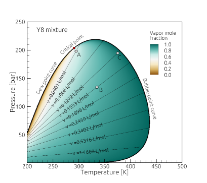
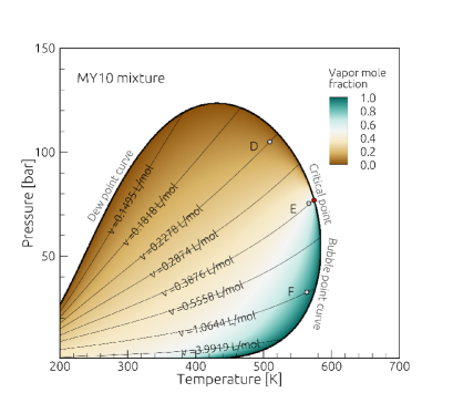
Two mixtures with specified compositions including a synthetic condensate gas and synthetic oil are selected in order to validate and evaluate the performance of proposed flash algorithms. The first fluid is the Y8 mixture introduced by Yarborough 27. It is a six-component synthetic gas condensate of normal alkanes including 80.9780.9780.97 C1, 5.665.665.66 C2, 3.063.063.06 C3, 4.574.574.57 nC5, 3.303.303.30 nC7, and 2.442.442.44 nC10 mole percents with a zero binary interaction matrix. With our reduction method, the latter results in only three governing equations for the reduced variables. The second fluid is the MY10 mixture introduced by Metcalfe and Yarborough 28. It is a ten-component mixture with overall molar fractions of 0.350.350.35 C1, 0.030.030.03 C2, 0.040.040.04 C3, 0.060.060.06 nC4, 0.040.040.04 nC5, 0.030.030.03 nC6, 0.050.050.05 nC7, 0.050.050.05 nC8, 0.300.300.30 nC10, and 0.050.050.05 nC14. For this mixture, all binary interaction coefficients are zero except those between the methane and the other components as reported by Firoozabadi and Pan 29. This sparse binary interaction matrix results in three non-zero eigenvalues λ1=9.9574subscript𝜆19.9574{\lambda_{1}}=9.9574, λ2=0.0707subscript𝜆20.0707{\lambda_{2}}=0.0707 and λ3=0.0280subscript𝜆30.0280{\lambda_{3}}=-0.0280.

Refer to caption
Refer to caption
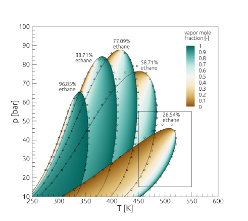
Figure 1: Phase diagrams for the Y8 and MY10 mixtures including isochores and the states selected for the detailed analysis of the convergence of the flash algorithms.
Refer to caption
Refer to caption
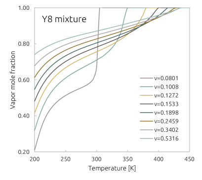
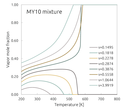
Figure 2: Vapor mole fraction curves as a function of temperature generated by the VT-flash algorithm corresponding to the lines shown in Fig. 1.

In Fig. 1, the phase diagrams for the two mixtures with contours of vapor mole fractions are shown. These diagrams are generated without any convergence problems of the blind PT-flashes over a fine Cartesian grid with 800×800800800800\times 800 nodes for the pressure - temperature range shown in the figure. This very fine grid is selected in order to check the applicability of the PT-flash algorithm at many different conditions very quite close to the phase boundaries and the critical point, where other methods may converge either very slowly or not at all.

Next, VT-flashes have been conducted along isochores drawn on the phase diagram. Selected isochoric lines are drawn in Fig. 1 to show the pressure evolution during constant volume heating or cooling of a typical condensate gas or synthetic oil. The corresponding vapor mole fraction curves shown in Fig. 2 were computed using the proposed VT-flash algorithm with the starting temperature of 200200200 [K] and a step size of 111 [K] up-to the saturation point. The retrograde behavior of MY10 for specific volumes lower than or equal to 0.28740.28740.2874 [L/mol] is an interesting phenomena: by increasing the temperature from 200200200 [K] the vapor mole fraction first increases with temperature and then decreases to zero. We verified that the results agree with our previous implementation of Michelson’s methods 3 and that the results of the VT-flashes are the same as those obtained with the PT-flashes up to machine round-off precision.

The performance of the isothermal and non-isothermal flash algorithms is investigated for six algorithmically challenging points (A-F) marked in the phase diagrams of the mixtures, see Fig. 1. The overall thermodynamic properties at these points are listed in Table 2 and results for the molar composition of the vapor and liquid in equilibrium are shown in Table 3. These values are equal for all types of flash calculations.
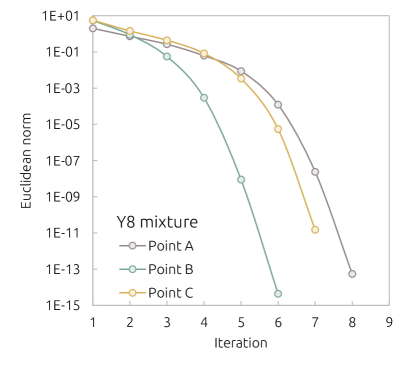
Refer to caption
Refer to caption
Figure 3: PT-flash convergence for the Y8 and MY10 mixtures at the points marked in Fig. 1.
Refer to caption
Refer to caption
Figure 4: VT-flash convergence for the Y8 and MY10 mixtures at the points marked in Fig. 1.
Refer to caption
Refer to caption
Figure 5: HP-flash convergence for the Y8 and MY10 mixtures at the points marked in Fig. 1.
Refer to caption
Refer to caption
Figure 6: UV-flash convergence for the Y8 and MY10 mixtures at the points marked in Fig. 1.

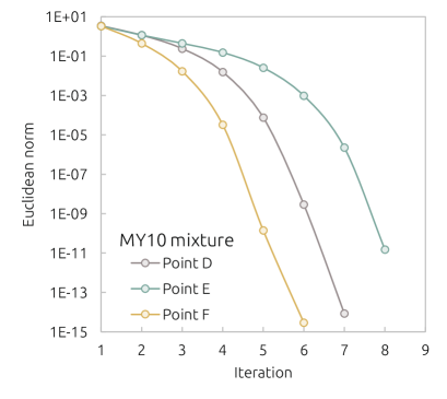
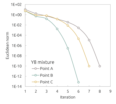
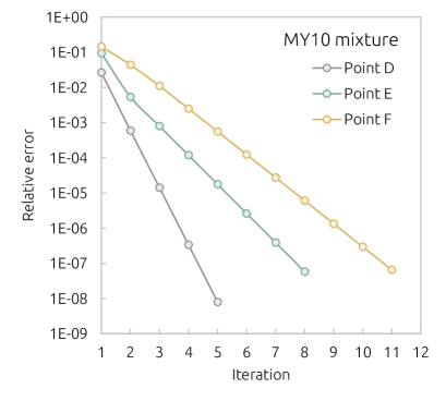
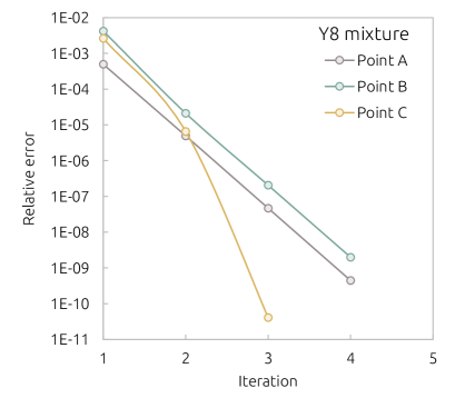
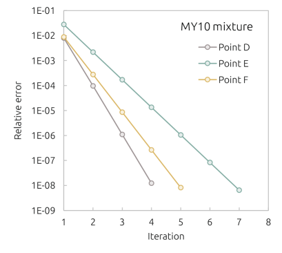
The evolution of the Euclidean residual norm for the PT-flash calculations at points A (198.1198.1198.1 [bar], 295.4295.4295.4 [K]), B (134.5134.5134.5 [bar], 335.2335.2335.2 [K]), and C (194.8194.8194.8 [bar], 375.3375.3375.3 [K]) for the Y8 mixture, and at points D (104.9104.9104.9 [bar], 509.1509.1509.1 [K]), E (75.475.475.4 [bar], 566.6566.6566.6 [K]), and F (32.732.732.7 [bar], 566.6566.6566.6 [K]) for the MY10 mixture are plotted in Fig. 3. For all points, one SSI has been carried out on the initial K-factors obtained from Wilson’s correlation before switching to the NRI. Results indicate that PT-flash algorithm requires about 68686-8 iterations for the points at the heart of the two-phase dome, near the phase boundaries, and close to the critical point.

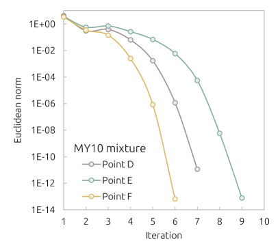
The convergence of the residuals of VT-flash calculations are shown in Fig. 4 for the points A (0.08060.08060.0806 [L/mol], 295.4295.4295.4 [K]), B (0.15330.15330.1533 [L/mol], 335.2335.2335.2 [K]), and C (0.12730.12730.1273 [L/mol], 375.3375.3375.3 [K]) corresponding to the marked points on the phase diagram of the Y8 mixture, and for the points D (0.22810.22810.2281 [L/mol], 509.1509.1509.1 [K]), E (0.38470.38470.3847 [L/mol], 566.6566.6566.6 [K]), and F (1.05961.05961.0596 [L/mol], 563.5563.5563.5 [K]) corresponding to the tagged points on the phase diagram of the MY10 mixture. Initial values for the K-factors were obtained from Wilson’s correlation using a pressure obtained from the state equation by the overall composition and given temperature and volumes, i.e. p={188.8,119.3,193.2,95.5,74.1,33.2}𝑝188.8119.3193.295.574.133.2p=\{188.8,119.3,193.2,95.5,74.1,33.2\} [bar] for points {{\{ A to F }}\}. As for the PT-flashes, one initial SSI was executed before switching to NRI. The VT-flash results show the same excellent convergence behavior as observed for the PT-flashes, that is, both algorithms have optimum quadratic convergence and require only very few iterations, with only two iterations difference between points close to and far from the extreme conditions.

Figure 5 shows the convergence of the relative errors for the blind HP-flash at points A (94.70494.704-94.704 [kJ/mol], 198.1198.1198.1 [bar]), B (90.63790.637-90.637 [kJ/mol], 134.5134.5134.5 [bar]), and C (87.89687.896-87.896 [kJ/mol], 194.8194.8194.8 [bar]) for the the condensate gas and at points D (142.741142.741-142.741 [kJ/mol], 104.9104.9104.9 [bar]), E (124.941124.941-124.941 [kJ/mol], 75.475.475.4 [bar]), and F (120.734120.734-120.734 [kJ/mol], 32.732.732.7 [bar]) for the synthetic oil. We initalize the iteration with a temperature of 250250250 [K] for Y8 and 400400400 [K] for MY10, far away from the true solution, in order to test the robustness of the non-isothermal flashes at extreme conditions. As the convergence plots show, they rapidly converge within very few iterations even with a poor inital temperature guess.

Figure 6 shows results for the blind UV-flash at the points A (96.30096.300-96.300 [kJ/mol], 0.08050.08050.0805 [L/mol]), B (92.69992.699-92.699 [kJ/mol], 0.15330.15330.1533 [L/mol]), and C (90.37690.376-90.376 [kJ/mol], 0.12730.12730.1273 [L/mol]) for Y8 and at the points D (145.134145.134-145.134 [kJ/mol], 0.22810.22810.2281 [L/mol]), E (127.841127.841-127.841 [kJ/mol], 0.38470.38470.3847 [L/mol]), and F (124.199124.199-124.199 [kJ/mol], 1.05961.05961.0596 [L/mol]) for the MY10 mixture. As before, the initial temperature guess is 250250250 [K] for the Y8 gas condensate and 400400400 [K] for the MY10 oil mixture. The initial values for the pressure are the same as used for the VT-flash at these points, see above. We observe rapid convergence within 4 to 7 iterations to within a relative error of 108superscript10810^{-8}. For the most of engineering applications, it is, however, not necessary to know the temperature with such a high precision and a much larger error, say 0.10.10.1 [K] can be tolerated. The algorithms for both non-isothermal flashes yield temperature differences of less than 0.10.10.1 [K] in just 333 iterations.

5.2 Computational time

Refer to caption
Figure 7: Phase diagram of binary mixtures of n-heptane and ethane at various molar compositions computed by the proposed algorithm. The symbols denote experimental reference data for the dew-point and bubble-point lines 30, 31. The black box encloses the pressure-temperature domain that was used for measuring the computational performance of the flash algorithms.
Refer to caption
Refer to caption
Figure 8: Computational time for PT-flashes and UV-flashes vs. number of mixture components. Shown is the total CPU time for 100×100100100100\times 100 flash calculations in the part of the phase diagram highlighted in Fig. 7.

In this section, we analyse the computational performance of the proposed flash algorithms for different mixtures and demonstrate the improved efficiency resulting from using a reduction method and direct VT-flashes instead of PT-flashes in the inner iteration loop of UV-flashes. For a fair quantitative evaluation, the computational time required for the new flash algorithms that we propose in this paper is compared with the highly optimized implementation of a conventional method that was developed by Matheis and Hickel 32 for the large-scale turbulence-resolving CFD simulations of transcritical fuel injection. Both algorithms use a Newton method to achieve fast convergence. The calculations are performed on an Intel Xeon W-2123 CPU at 3.60 GHz and the Intel Fortran compiler was used.

The test fluid is a mixture of ethane and normal heptane. The phase diagrams of this binary mixture for various molar compositions are shown in Fig. 7. To study the effect of the component number in the mixture, we have added pseudo-components with properties identical to ethane and normal heptane and adjust the mole fractions in a way that the total composition remains constant. First, PT-flash calculations were carried out for a mixture with 26.54%percent26.5426.54\% ethane and we record the total computational time 100×100100100100\times 100 states in the pressure-temperature range that is enclosed by the black box in Fig. 7. Then, the mixture internal energy and specific volume that were computed by the PT-flashes are used for executing the corresponding UV-flashes. In order to assess the performance of the proposed UV-flash at conditions that similar to what we typically encounter in CFD simulations, initial guesses of pressure and temperature were computed by adding random perturbations to the true values, that is:

Tguess=Ttrue+rΔT,subscript𝑇𝑔𝑢𝑒𝑠𝑠subscript𝑇𝑡𝑟𝑢𝑒𝑟Δ𝑇\displaystyle\begin{split}T_{guess}&={T_{true}}+r\Delta T\ ,\end{split} (76a)
pguess=ptrue+rΔp,subscript𝑝𝑔𝑢𝑒𝑠𝑠subscript𝑝𝑡𝑟𝑢𝑒𝑟Δ𝑝\displaystyle\begin{split}p_{guess}&={p_{true}}+r\Delta p\ ,\end{split} (76b)

where r𝑟r is a random number generated in the range [0.5,0.5]0.50.5[-0.5,0.5]. The perturbation amplitudes ΔTΔ𝑇\Delta T and ΔpΔ𝑝\Delta p are set to 202020 [K] and 202020 kPa, which corresponds to the maximum change that we can expect between two subsequent time steps in CFD simulations.

The results are shown in Fig. 8. The computational time for the current PT-flash algorithm is always lower than the highly optimized reference method. The difference becomes more significant as the number of components is increased, which shows the importance of reduction methods for the both iso-thermal and non-isothermal flashes. Surprisingly, we also measure a performance gain for the two-component mixture, where the number of variables is not reduced by the new method. In this case, the reduction method acts as a preconditioner and reduces the number of required iterations for the PT-flash. Furthermore, it should be noted that the computational performance the UV-flash based on the VT-flash is much less sensitive to the amplitude of the imposed pressure perturbation ΔpΔ𝑝\Delta p than the conventional method based on the PT-flash. For instance, the conventional method becomes more than five times slower for Δp=400Δ𝑝400\Delta p=400 kPa, whereas the overall time needed for the new method remains unchanged.

6 Discussion and Conclusions

This work was motivated by the need for computationally efficient and very robust vapor-liquid phase-split calculations in turbulence-resolving CFD simulations of high-pressure liquid-fuel injection and reacting transcritical multiphase flows in modern energy conversion systems, such as rocket engines, gas turbines and jet engines. Such simulations require typically 1010superscript101010^{10} to 1016superscript101610^{16} flash calculations for given overall specific internal energy, volume and composition and unknown pressure, temperature, volume fractions and phase compositions (isoenergetic-isochoric flash – UV-flash). The standard methods for such applications that we used in the past 32, 3 are based on a nested PT-flash and suffer from poor conditioning near the spinodal and coexistence curves and polynomial growth of the computational cost in terms of the number of mixture components. To this end, and building upon and extending the work of Mikyška and Firoozabadi 16 and Nichita and Graciaa 15, we have developed a new multi-component reduction method for direct PT-flash and VT-flash calculations based on the formulation of phase equilibrium conditions in terms of the molar specific value of Mikyška and Firoozabadi’s volume function and a corresponding adaptation of Nichita and Graciaa’s reduction method. The computational cost of solving the PT-flash and VT-flash in terms of the new reduced set of variables is almost independent of the number of components and the point in the phase diagram. The reduced-space Newton-Raphson iteration, using the exact analytical Jacobian matrix, results in optimum quadratic convergence in very few iterations. We further showed that the non-isothermal UV and HP flashes are efficiently solved through univariate residual minimization with the naturally corresponding isothermal flash (PT-flash for HP-flash and VT-flash for UV-flash) and the specific heat capacity at constant pressure (for HP-flash) or at constant volume (for UV-flash) as exact Jacobian. We have thoroughly verified the reliability and efficiency of the algorithmic implementation. The computational results show a considerable speed-up compared to conventional methods, as well as improved robustness and better convergence behavior near the spinodal and coexistence curves of multi-component mixtures, where the preconditioning by the reduction method is most effective.

Acknowledgements

This work is funded by the Netherlands Organisation for Scientific Research (Contract No. 680.91.082).

References

  • Rongy et al. 2012 Laurence Rongy, Kjetil B Haugen, and Abbas Firoozabadi. Mixing from Fickian diffusion and natural convection in binary non-equilibrium fluid phases. AIChE Journal, 58(5):1336–1345, 2012.
  • Polívka and Mikyška 2014 Ondřej Polívka and Jiří Mikyška. Compositional modeling in porous media using constant volume flash and flux computation without the need for phase identification. Journal of Computational Physics, 272:149 – 169, 2014.
  • Matheis and Hickel 2018 Jan Matheis and Stefan Hickel. Multi-component vapor-liquid equilibrium model for LES of high-pressure fuel injection and application to ECN Spray A. International Journal of Multiphase Flow, 99:294–311, 2018.
  • Ma et al. 2019 Peter C. Ma, Hao Wu, Daniel T. Banuti, and Matthias Ihme. On the numerical behavior of diffuse-interface methods for transcritical real-fluids simulations. International Journal of Multiphase Flow, 113:231 – 249, 2019.
  • Rodriguez et al. 2019 Carlos Rodriguez, Houman B Rokni, Foivos Koukouvinis, Ashutosh Gupta, and Manolis Gavaises. Complex multicomponent real-fluid thermodynamic model for high-pressure Diesel fuel injection. Fuel, 257:115888, 2019.
  • Tudisco and Menon 2020 Principio Tudisco and Suresh Menon. Numerical Investigations of Phase-Separation During Multi-Component Mixing at Super-Critical Conditions. Flow, Turbulence and Combustion, 104(2):(in press), 2020.
  • Abhvani et al. 1987 AS Abhvani, DN Beaumont, et al. Development of an efficient algorithm for the calculation of two-phase flash equilibria. SPE Reservoir Engineering, 2(04):695–702, 1987.
  • Michelsen 1998 Michael L. Michelsen. Speeding up the two-phase PT-flash, with applications for calculation of miscible displacement. Fluid Phase Equilibria, 143(1):1 – 12, 1998.
  • Michelsen 1982a Michael L Michelsen. The isothermal flash problem. Part I. Stability. Fluid phase equilibria, 9(1):1–19, 1982a.
  • Michelsen 1982b Michael L Michelsen. The isothermal flash problem. Part II. Phase-split calculation. Fluid phase equilibria, 9(1):21–40, 1982b.
  • Michelsen 1999 Michael L Michelsen. State function based flash specifications. Fluid Phase Equilibria, 158:617–626, 1999.
  • Michelsen 1986 Michael L Michelsen. Simplified flash calculations for cubic equations of state. Industrial & Engineering Chemistry Process Design and Development, 25(1):184–188, 1986.
  • Petitfrere and Nichita 2015 Martin Petitfrere and Dan Vladimir Nichita. A comparison of conventional and reduction approaches for phase equilibrium calculations. Fluid Phase Equilibria, 386:30–46, 2015.
  • Hendriks and Van Bergen 1992 EM Hendriks and ARD Van Bergen. Application of a reduction method to phase equilibria calculations. Fluid Phase Equilibria, 74:17–34, 1992.
  • Nichita and Graciaa 2011 Dan Vladimir Nichita and Alain Graciaa. A new reduction method for phase equilibrium calculations. Fluid Phase Equilibria, 302(1-2):226–233, 2011.
  • Mikyška and Firoozabadi 2011 Jiří Mikyška and Abbas Firoozabadi. A new thermodynamic function for phase-splitting at constant temperature, moles, and volume. AIChE Journal, 57(7):1897–1904, 2011.
  • Jindrová and Mikyška 2015 Tereza Jindrová and Jiří Mikyška. General algorithm for multiphase equilibria calculation at given volume, temperature, and moles. Fluid Phase Equilibria, 393:7–25, 2015.
  • Nichita 2018 Dan Vladimir Nichita. New unconstrained minimization methods for robust flash calculations at temperature, volume and moles specifications. Fluid Phase Equilibria, 466:31–47, 2018.
  • Cismondi et al. 2018 Martin Cismondi, Papa Matar Ndiaye, and Frederico W Tavares. A new simple and efficient flash algorithm for Tv specifications. Fluid Phase Equilibria, 464:32–39, 2018.
  • Firoozabadi 2015 Abbas Firoozabadi. Thermodynamics and Applications of Hydrocarbons Energy Production. McGraw-Hill Professional, 2015.
  • Michelsen and Mollerup 2007 Michael Locht Michelsen and Jørgen Mollerup. Thermodynamic Models: Fundamentals and Computational Aspects. Tie-Line Publications, 2007.
  • Nichita and Petitfrere 2013 Dan Vladimir Nichita and Martin Petitfrere. Phase stability analysis using a reduction method. Fluid Phase Equilibria, 358:27–39, 2013.
  • Goos et al. 2009 Elke Goos, Alexander Burcat, and Branko Ruscic. Third millennium ideal gas and condensed phase thermochemical database for combustion. URL: http://garfield.chem.elte.hu/Burcat/burcat.html, 2009.
  • Mikyška and Firoozabadi 2012 Jiří Mikyška and Abbas Firoozabadi. Investigation of mixture stability at given volume, temperature, and number of moles. Fluid Phase Equilibria, 321:1–9, 2012.
  • Nichita 2017 Dan Vladimir Nichita. Fast and robust phase stability testing at isothermal-isochoric conditions. Fluid Phase Equilibria, 447:107–124, 2017.
  • Nichita and Leibovici 2013 Dan Vladimir Nichita and Claude F Leibovici. A rapid and robust method for solving the Rachford–Rice equation using convex transformations. Fluid Phase Equilibria, 353:38–49, 2013.
  • Yarborough 1972 Lyman Yarborough. Vapor-liquid equilibrium data for multicomponent mixtures containing hydrocarbon and nonhydrocarbon components. Journal of Chemical and Engineering Data, 17(2):129–133, 1972.
  • Metcalfe and Yarborough 1979 Richard S Metcalfe and Lyman Yarborough. The effect of phase equilibria on the CO2 displacement mechanism. SPE Journal, 19(04):242–252, 1979.
  • Firoozabadi and Pan 2002 Abbas Firoozabadi and Huanquan Pan. Fast and robust algorithm for compositional modeling: Part I - stability analysis testing. SPE Journal, 7(1):78–89, 2002.
  • Kay 1938 W B Kay. Liquid-vapor phase equilibrium relations in the Ethane- n-Heptane system. Industrial and Engineering Chemistry, 30(4):459–465, April 1938.
  • Mehra and Thodos 1965 Vinod S Mehra and George Thodos. Vapor-liquid equilibrium in the Ethane-n-Heptane system. Journal of Chemical and Engineering Data, 10(3):211–214, July 1965.
  • Matheis and Hickel 2016 Jan Matheis and Stefan Hickel. Multi-component vapor-liquid equilibrium model for LES and application to ECN Spray A. In Studying Turbulence UsingNumerical SimulationDatabases - XVI – Proceedings of the 2016 Summer Program, pages 25–34. Center for Turbulence Research, Stanford University, 2016.