Time evolution of entanglement negativity across a defect

Abstract

We consider a quench in a free-fermion chain by joining two homogeneous half-chains via a defect. The time evolution of the entanglement negativity is studied between adjacent segments surrounding the defect. In case of equal initial fillings, the negativity grows logarithmically in time and essentially equals one-half of the Rényi mutual information with index $\alpha=1/2$ in the limit of large segments. In sharp contrast, in the biased case one finds a linear increase followed by the saturation at an extensive value for both quantities, which is due to the backscattering from the defect and can be reproduced in a quasiparticle picture. Furthermore, a closer inspection of the subleading corrections reveals that the negativity and the mutual information have a small but finite difference in the steady state. Finally, we also study a similar quench in the XXZ spin chain via density-matrix renormalization group methods and compare the results for the negativity to the fermionic case.

I Introduction

The study of integrable quantum many-body systems out of equilibrium has received considerable attention in the last decade Calabrese et al. (2016). Among the various research directions, the identification of the stationary ensemble Vidmar and Rigol (2016) towards which the system locally relaxes after a quantum quench Essler and Fagotti (2016) is of central importance. In understanding the mechanisms of this relaxation and equilibration, a crucial role is played by entanglement dynamics. In particular, the buildup of an extensive subsystem entropy can be traced back to the propagation of entangled quasiparticle excitations created by the quench Calabrese and Cardy (2005); Alba and Calabrese (2017).

The situation is, however, less clear if the translational invariance of the Hamiltonian governing the dynamics is broken by the presence of an impurity. In the generic case, such a local deformation typically destroys the integrability of the model, which makes the study of the dynamics far more complicated. Hence, most of our understanding about entanglement evolution across a defect is essentially restricted to free-fermion systems. These studies include free-fermion chains with a simple hopping defect Klich and Levitov (2009); Song et al. (2012); Eisler and Peschel (2012); Gamayun et al. (2020), the transverse Ising chain with a coupling defect Iglói et al. (2009), and even some more complicated interacting defects between non-interacting leads Kennes et al. (2014); Vasseur and Saleur (2017); Bidzhiev and Misguich (2017); He and Millis (2017).

In general, the behaviour of the half-chain entanglement depends crucially on whether a density bias is applied between the fermionic leads separated by the defect. For the unbiased case, one finds a logarithmic growth of entanglement, with the same prefactor that governs the equilibrium entropy scaling in the presence of a defect, which was studied both numerically and analytically for hopping chains Peschel (2005); Eisler and Peschel (2010); Eisler and Garmon (2010); Peschel and Eisler (2012); Arias (2020) as well as in the continuum Calabrese et al. (2011); Calabrese et al. (2012a). The exact same relation can actually be found in conformal field theory (CFT) calculations Wen et al. (2018), connecting entropy dynamics after the quench to the problem of ground-state entanglement across a conformal interface Sakai and Satoh (2008); Brehm and Brunner (2015). In sharp contrast, entanglement was found to grow linearly if a density bias is applied to the leads, which can be attributed to backscattering from the defect Eisler and Peschel (2012).

The examples mentioned above deal with a bipartite setting, where the entanglement entropy is calculated between two halves of the chain, with the defect located in the center. It is natural to ask how the results are modified when entanglement is considered between two finite segments surrounding the defect. Since the reduced state of the two segments is not any more pure, the Rényi entropies are no longer measures of entanglement. In such a tripartite geometry, a possible way of quantifying entanglement is via the logarithmic negativity Vidal and Werner (2002); Plenio (2005). In homogeneous systems, the time evolution of the entanglement negativity has already been considered in a similar geometry for global Coser et al. (2014); Alba and Calabrese (2019) or local quenches Wen et al. (2015); Feldman and Goldstein (2019), and even for initial states with a temperature or density bias Eisler and Zimborás (2014); Hoogeveen and Doyon (2015); Gullans and Huse (2019). Particularly interesting are the recent results of Ref. Alba and Calabrese (2019), where a nontrivial relation between the entanglement negativity and the Rényi mutual information with index $\alpha=1/2$, measured between two neighbouring blocks, has been established for free-particle systems after a global quench.

In the present paper we shall study the time evolution of the entanglement across a defect by employing a fermionic version of the logarithmic negativity introduced in Shapourian et al. (2017). One of the main questions we address is whether the relation between entanglement negativity and Rényi mutual information still holds in such an inhomogeneous quench problem. For the unbiased quench the answer is positive, with the functional form of the entanglement evolution being well approximated by that after a homogeneous local quench Wen et al. (2015), with an effective central charge that follows from the ground-state defect problem. In case of a density bias, the leading order behaviour is again the same for both quantities and can be captured by a semiclassical picture, similar to the one applied for the half-chain entropy Eisler and Peschel (2012). Here the pairs of partially reflected and transmitted single-particle excitations created at the defect contribute to a linear buildup of entanglement, which eventually saturates at an extensive value. However, the subleading corrections for the entanglement negativity and mutual information are found to differ by a finite amount in the steady state, even in the limit of large segments. Finally, we also study the standard logarithmic negativity for the XXZ chain with a single coupling defect in a similar quench setup, using the numerical methods introduced in Ruggiero et al. (2016). In particular, for the XX chain that is very closely related to the hopping chain, we find that the spin-chain negativity is always upper-bounded by the fermionic one.

The manuscript is structured as follows. In Section II we introduce the basic setup and the method of calculating the Rényi mutual information and logarithmic negativity for fermionic Gaussian states. In Sec. III we discuss the entanglement negativity in the ground state of a chain with a defect. Sections IV and V are devoted to the study of the quench from equal and unequal fillings, respectively. In Sec. VI we compute the negativity after a quench in the XXZ chain with a defect. We conclude with a discussion of our results in VII, followed by two Appendices providing some technical details of the calculations.

II Model and methods

We consider a chain of noninteracting fermions with a single hopping defect, described by the Hamiltonian

$$\hat{H}=\hat{H}_{l}+\hat{H}_{r}-\frac{\lambda}{2}\left(f_{0}^{\dagger}f_{1}+f_{1}^{\dagger}f_{0}\right),$$ (1)

where the hopping amplitude $\lambda$ characterizes the defect in the middle of the chain, while the homogeneous half-chains on the left/right hand side of the defect are given by

$$\hat{H}_{l}=-\frac{1}{2}\sum_{j=-N+1}^{-1}\left(f_{j}^{\dagger}f_{j+1}+f_{j+1}^{\dagger}f_{j}\right)\,,\qquad\hat{H}_{r}=-\frac{1}{2}\sum_{j=1}^{N-1}\left(f_{j}^{\dagger}f_{j+1}+f_{j+1}^{\dagger}f_{j}\right)\,.$$ (2)

The full chain has $2N$ sites and the fermionic annihilation (creation) operators $f_{j}$ ($f_{j}^{\dagger}$) with $j=-N+1,\dots,N$ satisfy the canonical anticommutation relation $\{f_{i},f_{j}^{\dagger}\}=\delta_{ij}$. The defect $\lambda\leq 1$ is assumed to be weaker than the tunneling in the leads $\hat{H}_{l}$ and $\hat{H}_{r}$.

In the following sections we shall either consider the ground state or the time evolution generated by (1). In the latter case, the chain is initially split in two halves and our quench protocol is depicted in Fig. 1. Here the initial state $\ket{\psi_{\sigma}}$ of the left/right part ($\sigma=l,r$) is given by the respective ground state of $\hat{H}_{\sigma}-\mu_{\sigma}\sum_{j\in\sigma}f_{j}^{\dagger}f_{j}$, where the chemical potential $\mu_{\sigma}$ sets the filling $n_{\sigma}$ of the corresponding half-chain. In particular, one sets $\mu_{l}=\mu_{r}=0$ to initialize both chains in their half-filled ground states $n_{l}=n_{r}=1/2$, whereas the choice $\mu_{l}=1$ and $\mu_{r}=-1$ corresponds to the step-like density $n_{l}=1$ and $n_{r}=0$ (also known as the domain wall initial state). In either case, the two halves are then coupled via a defect, depicted by the dashed bond in Fig. 1, and the resulting unitary time evolution is given by

$$\ket{\psi(t)}=e^{-i\hat{H}t}\ket{\psi_{l}}\otimes\ket{\psi_{r}}\,.$$ (3)

We are primarily interested in the buildup of entanglement in the time-evolved state $\ket{\psi(t)}$, between two segments $A_{1}$ and $A_{2}$ as shown by the colored sites in Fig. 1. We restrict ourselves to the case of adjacent segments of equal lengths $\ell$, located symmetrically around the defect. The bipartite case of $\ell=N$ ($B=\emptyset$) was studied in Ref. Eisler and Peschel (2012), where the entanglement in the pure state $\rho=\ket{\psi(t)}\bra{\psi(t)}$ is simply measured by the Rényi entropies between the two halves. In general, however, one has to first extract the reduced density matrix $\rho_{A}=\mathrm{Tr}_{B}(\rho)$ of the subsystem $A=A_{1}\cup A_{2}$ by tracing out over the environment $B$. This leaves us with a mixed state where the entanglement is much harder to be quantified and requires a proper measure.

Figure 1: Quench setup.

Before introducing this measure, one should remark that the time-evolved state (3) is Gaussian and thus fully characterized by its correlation matrix $C_{mn}(t)=\bra{\psi(t)}f_{m}^{\dagger}f_{n}\ket{\psi(t)}$. Indeed, since we are dealing with free fermions, the Hamiltonian (1) can be written in the quadratic form

$$\hat{H}=\sum_{m,n}H_{m,n}f_{m}^{\dagger}f_{n}\,,$$ (4)

which defines the elements $H_{m,n}$ of the hopping matrix $H$. Then the time evolution of the correlation matrix can simply be obtained as

$$C(t)=e^{iHt}\,C(0)\,e^{-iHt}\,.$$ (5)

The initial correlation matrix of the decoupled system at $t=0$ has a block-diagonal form

$$C(0)=\left(\begin{array}[]{cc}C_{l}&0\\ 0&C_{r}\end{array}\right),$$ (6)

where $C_{\sigma}$ is the ground-state correlation matrix at filling $n_{\sigma}$, with matrix elements given by Fagotti and Calabrese (2011)

$$(C_{\sigma})_{m,n}=\frac{1}{2(N+1)}\left[\frac{\sin(q_{F,\sigma}(m-n))}{\sin(\frac{\pi}{2(N+1)}(m-n))}-\frac{\sin(q_{F,\sigma}(m+n))}{\sin(\frac{\pi}{2(N+1)}(m+n))}\right],$$ (7)

and the Fermi wavenumber is defined as

$$q_{F,\sigma}=\frac{\pi(n_{\sigma}\,N+1/2)}{N+1}\,.$$ (8)

In particular, half-filling $n_{\sigma}=1/2$ corresponds to a Fermi momentum $q_{F,\sigma}=\pi/2$, whereas for the step initial condition ($n_{l}=1,\,n_{r}=0$) the correlations simplify to $(C_{l})_{m,n}=\delta_{m,n}$ and $(C_{r})_{m,n}=0$

II.1 Rényi entropy and mutual information

For the pure state $\rho=\ket{\psi(t)}\bra{\psi(t)}$, the reduced density matrix of the segment $A_{1}$ is given by $\rho_{A_{1}}=\mathrm{Tr}_{B\cup A_{2}}(\rho)$. The Rényi entropy between the segment $A_{1}$ and the rest of the system is defined as

$$S_{\alpha}(\rho_{A_{1}})=\frac{1}{1-\alpha}\ln\mathrm{Tr}\,(\rho^{\alpha}_{A_{1}})\,,$$ (9)

with the von Neumann entropy corresponding to the limit $\alpha=1$. Note, however, that these measures do not give information about the entanglement between $A_{1}$ and $A_{2}$. To gain some insight about the latter, one could consider the Rényi mutual information defined by the combination of subsystem entropies

$$\mathcal{I}_{\alpha}=S_{\alpha}(\rho_{A_{1}})+S_{\alpha}(\rho_{A_{2}})-S_{\alpha}(\rho_{A})\,.$$ (10)

The standard (von Neumann) mutual information with $\alpha=1$ is known to be a measure of total (classical and quantum) correlations and is thus an upper bound to the entanglement Groisman et al. (2005). Unfortunately, however, for generic $\alpha$ it is not even a proper measure. Indeed, it was demonstrated that $\mathcal{I}_{\alpha}$ may become negative for $\alpha>2$ after a certain quench Kormos and Zimborás (2017). On the other hand, it has been proved that $\mathcal{I}_{\alpha}$ is always positive in the range $0<\alpha<2$ for both fermionic and bosonic Gaussian states Camilo et al. (2019). Furthermore, recently it was pointed out that the particular case $\alpha=1/2$ is intimately related to a proper entanglement measure, the logarithmic negativity (see below), after a global quench Alba and Calabrese (2019). Thus our focus will be exclusively on the case $\alpha=1/2$.

The Rényi mutual information (10) is a simple combination of bipartite entropies in the pure Gaussian state $\rho$ and is thus uniquely determined by the correlation matrix (5). In particular, for the segment $A_{1}$ one has

$$S_{\alpha}(\rho_{A_{1}})=\frac{1}{1-\alpha}\sum_{j}\ln\left[\zeta_{j}^{\alpha}+(1-\zeta_{j})^{\alpha}\right],$$ (11)

where $\zeta_{j}$ are the eigenvalues of the reduced correlation matrix $C_{A_{1}}(t)$, with indices restricted to the segment $m,n\in A_{1}$. Similar expressions hold for the other terms in the mutual information (10), where the eigenvalues of the respective reduced correlation matrices $C_{A_{2}}(t)$ and $C_{A}(t)$ must be used.

II.2 Entanglement negativity

The logarithmic negativity is a versatile measure of entanglement Vidal and Werner (2002). Its definition relies on the partial transpose of the density matrix, which may have negative eigenvalues only if the system is entangled Peres (1996). For bosonic systems, the effect of the partial transpose is well known to be identical to a partial time reversal Simon (2000). However, for fermionic systems this is not any more the case. Indeed, in contrast to partial time reversal Shapourian et al. (2017), the partial transpose in general does not lead to a Gaussian operator Eisler and Zimborás (2015). However, it has been proved that the definition based on partial time reversal also yields a proper measure of entanglement Shapourian and Ryu (2019). Therefore, we shall adopt here the fermionic version of the logarithmic negativity, since it is directly amenable to correlation-matrix techniques.

In order to define the fermionic negativity, it is more convenient to work in the Majorana operator basis

$$c_{2j-1}=f_{j}+f_{j}^{\dagger},\qquad c_{2j}=i(f_{j}-f_{j}^{\dagger})\,,$$ (12)

satisfying the anticommutation relations $\{c_{m},c_{n}\}=2\delta_{mn}$. We can now expand the reduced density matrix $\rho_{A}$ supported on the segment $A=A_{1}\cup A_{2}$ encompassing the defect (see Fig. 1) as

$$\rho_{A}=\sum_{\begin{subarray}{c}\kappa,\tau\\ |\kappa|+|\tau|=\text{even}\end{subarray}}w_{\kappa,\tau}c_{-2\ell+1}^{\kappa_{1}}\dots c_{0}^{\kappa_{2\ell}}c_{1}^{\tau_{1}}\dots c_{2\ell}^{\tau_{2\ell}}\,.$$ (13)

Here $\kappa_{j}$ and $\tau_{j}$ with $j=1,\dots,2\ell$ are bit strings associated to the subspaces $A_{1}$ and $A_{2}$, with their norms defined as $|\kappa|=\sum_{j}\kappa_{j}$ and $|\tau|=\sum_{j}\tau_{j}$, respectively. The bit strings indicate whether a Majorana operator is included or not, $c_{j}^{0}=\mathbb{1}$ or $c_{j}^{1}=c_{j}$, with the weight of the corresponding term in the expansion given by $w_{\kappa,\tau}$. Importantly, the sum is restricted to terms, where the overall number of Majorana operators is even, reflecting the global fermion-number parity symmetry of the state.

The partial time reversal $R_{2}$ with respect to $A_{2}$ acts as Shapourian et al. (2017)

$$\rho_{A}^{R_{2}}=O_{+}=\sum_{\begin{subarray}{c}\kappa,\tau\\ |\kappa|+|\tau|=\text{even}\end{subarray}}w_{\kappa,\tau}i^{|\tau|}c_{-2\ell+1}^{\kappa_{1}}\dots c_{0}^{\kappa_{2\ell}}c_{1}^{\tau_{1}}\dots c_{2\ell}^{\tau_{2\ell}}\,,$$ (14)

where we have introduced the shorthand notation $O_{+}$ which will be useful also for the definition of the partial transpose. Note that, in general, $O_{+}$ is not a Hermitian operator and its conjugate will be denoted by $O_{-}=O_{+}^{\dagger}$. The fermionic logarithmic negativity is then defined as

$$\mathcal{E}_{f}=\ln\|\rho_{A}^{R_{2}}\|_{1}=\ln\mathrm{Tr}\sqrt{O_{+}O_{-}}\,.$$ (15)

Our goal is now to calculate $\mathcal{E}_{f}$ via the Majorana covariance matrix

$$\Gamma_{mn}=\frac{1}{2}\mathrm{Tr}\left(\rho\left[c_{m},c_{n}\right]\right),$$ (16)

where $\rho$ is the density matrix obtained from the pure state (3) as before. Since the dynamics conserves the fermion number, the covariance matrix $\Gamma$ is completely determined by $C(t)$ obtained from (5). Using the definition (12), it is easy to show that the following relations hold

$$\Gamma_{2j-1,2l}=-\Gamma_{2j,2l-1}=i\left(2\,C_{jl}(t)-\delta_{jl}\right)\,,\qquad\Gamma_{2j-1,2l-1}=\Gamma_{2j,2l}=2i\,\mathrm{Im}(C_{jl}(t))\,.$$ (17)

Note that we have suppressed the explicit $t$-dependence of the $\Gamma$ matrix for notational simplicity. Due to the Gaussianity of the state, the reduced density matrix $\rho_{A}$ is characterized by the reduced covariance matrix $\Gamma_{A}$. Moreover, one can show that $O_{\pm}$ are both Gaussian operators, with corresponding covariance matrix elements

$$(\Gamma_{\pm})_{mn}=\frac{1}{2}\mathrm{Tr}\left(O_{\pm}[c_{m},c_{n}]\right),$$ (18)

that can be written in the block form Eisler and Zimborás (2015); Shapourian et al. (2019)

$$\Gamma_{\pm}=\left(\begin{array}[]{cc}\Gamma_{A_{1}A_{1}}&\pm i\,\Gamma_{A_{1}A_{2}}\\ \pm i\,\Gamma_{A_{2}A_{1}}&-\Gamma_{A_{2}A_{2}}\end{array}\right),$$ (19)

where the block indices $A_{1}$ and $A_{2}$ denote the corresponding submatrices of $\Gamma_{A}$.

Clearly, evaluating the entanglement negativity in (15) boils down to an exercise of multiplying Gaussian operators and taking their trace. This has been carried out in Ref. Eisert et al. (2018) by introducing the auxiliary density matrix

$$\rho_{\times}=\frac{O_{+}O_{-}}{\mathrm{Tr}\,(O_{+}O_{-})},$$ (20)

which is a normalized Gaussian state with a real spectrum. Using the multiplication rules of Gaussian states, one can show that the corresponding covariance matrix can be written as Eisert et al. (2018)

$$\Gamma_{\times}\simeq\left(\frac{\mathbb{1}+\Gamma_{A}^{\,2}}{2}\right)^{-1}\left(\begin{array}[]{cc}\Gamma_{A_{1}A_{1}}&0\\ 0&-\Gamma_{A_{2}A_{2}}\end{array}\right),$$ (21)

where $\simeq$ denotes equality up to a similarity transformation. Indeed, it turns out that the result for $\mathcal{E}_{f}$ depends only on the spectra $\{\pm\nu_{j}^{\times}\}$ of $\Gamma_{\times}$ as well as that $\{\pm\nu_{j}\}$ of $\Gamma_{A}$, where $j=1,\dots,2\ell$ and the eigenvalues come in pairs due to the antisymmetry of the covariance matrix. The traces appearing in $\mathcal{E}_{f}$ can then be evaluated as

$$\mathrm{Tr}\,(O_{+}O_{-})=\mathrm{Tr}\,(\rho^{2}_{A})=\prod_{j=1}^{2\ell}\frac{1+\nu_{j}^{2}}{2}\,,\qquad\mathrm{Tr}\,(\rho^{1/2}_{\times})=\prod_{j=1}^{2\ell}\left[\left(\frac{1+\nu^{\times}_{j}}{2}\right)^{1/2}+\left(\frac{1-\nu^{\times}_{j}}{2}\right)^{1/2}\right].$$ (22)

Finally, using the formula (9) for the Rényi entropies, the logarithmic negativity can be put in the suggestive form

$$\mathcal{E}_{f}=\frac{1}{2}\left[S_{1/2}(\rho_{\times})-S_{2}(\rho_{A})\right].$$ (23)

We have thus obtained $\mathcal{E}_{f}$ as a combination of Rényi entropies of the reduced density matrix $\rho_{A}$ and the auxiliary density matrix $\rho_{\times}$, which in turn can be evaluated using the trace formulas (22). Note that, since the covariance matrix $\Gamma_{\times}$ is equivalent to the one in (21) which depends only on the matrix elements of $\Gamma_{A}$, the negativity is uniquely determined by the fermionic correlation matrix via (17). It is instructive to check the limit when $\rho_{A}$ corresponds to a pure state, such that $\Gamma^{2}_{A}=\mathbb{1}$ and one has trivially $S_{2}(\rho_{A})=0$. Furthermore, from (21) one observes that $\Gamma_{\times}$ becomes block diagonal and thus $S_{1/2}(\rho_{\times})=S_{1/2}(\rho_{A_{1}})+S_{1/2}(\rho_{A_{2}})$. Substituting into (23) and using the symmetry property $S_{1/2}(\rho_{A_{1}})=S_{1/2}(\rho_{A_{2}})$ of the Rényi entropy, one obtains the well known relation $\mathcal{E}_{f}=S_{1/2}(\rho_{A_{1}})$.

III Ground state entanglement

Although the main focus of our work is the time evolution of the entanglement across a defect, it turns out to be very useful to have a look at the ground-state entanglement first. Namely, we shall consider here the ground state of the chain (1) and calculate the entanglement negativity for the same geometry as for the quench shown in Fig. 1, i.e. for two equal segments surrounding the defect. In fact, in the bipartite case when the segment is taken to be the half-chain $(B=\emptyset)$, it has been shown that the entanglement entropies in the ground state and after the quench are very closely related Eisler and Peschel (2012); Wen et al. (2018).

The defect problem for the entanglement was first studied in Ref. Peschel (2005) where a single interval neighbouring the defect was considered in an infinite chain. The logarithmic scaling of the entropy was found to persist, albeit with a prefactor (dubbed as effective central charge) that varies continuously with the defect strength. Importantly, the contributions to the entanglement from the two boundaries of the interval were found to be additive. An analytical expression for the defect contribution was later derived in Eisler and Peschel (2010) by considering the half-chain entropy for $\alpha=1$, and further exact results for various other $\alpha$ were obtained in Peschel and Eisler (2012).

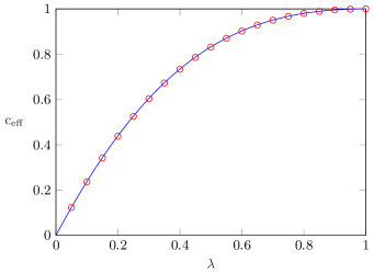
We shall now argue that the effective central charge for $\alpha=1/2$ will govern also the scaling of the entanglement negativity. Obviously, for the bipartite case this follows immediately from the relation $\mathcal{E}_{f}=S_{1/2}(\rho_{A_{1}})=\frac{1}{2}\,\mathcal{I}_{1/2}$. However, even in the generic tripartite case, one expects that the negativity should only be sensitive to the defect contribution. Indeed, $\mathcal{E}_{f}$ measures the entanglement between the segments $A_{1}$ and $A_{2}$ and should not care about the contribution of the homogeneous boundaries between $A$ and $B$. Now, this is exactly the contribution contained in $S_{1/2}(\rho_{A})$, which is subtracted in the mutual information. Indeed, as shown in Ossipov (2014), in the limit of $\ell\gg 1$, the Rényi entropy of an interval containing the defect in the middle is just given by the homogeneous result. Therefore, in complete analogy to Alba and Calabrese (2019), we assume by a continuity argument that the relation $\mathcal{E}_{f}\simeq\frac{1}{2}\,\mathcal{I}_{1/2}$ should hold in the tripartite case as well. Note that the factor $1/2$ just compensates the double counting of the defect contribution.

(a)

(b)

Figure 2: Left: comparison of the fits for $c_{\mathrm{eff}}$ (circles) according to Eq. (26), to the analytical formula (25) (line). Right: difference of $\mathcal{E}_{f}$ and $\frac{1}{2}\mathcal{I}_{1/2}$ as a function of $\ell$ for different coupling strengths $\lambda$.

One can now use the results for the $\alpha=1/2$ Rényi entropy to put forward the ansatz for the negativity

$$\mathcal{E}_{f}\simeq\frac{1}{2}\,\mathcal{I}_{1/2}=\frac{c_{\mathrm{eff}}}{4}\ln(\ell)+\mathrm{const},$$ (24)

where the effective central charge reads Peschel and Eisler (2012)

$$c_{\mathrm{eff}}=\frac{4}{\pi^{2}}\arcsin{(}s)(\pi-\arcsin{(}s))\,,\qquad s=\frac{2}{\lambda+\lambda^{-1}}\,.$$ (25)

Here $s$ is the transmission amplitude of the defect at the Fermi level $q_{F}=\pi/2$, i.e. the square root of the transmission coefficient $s=\sqrt{T_{q_{F}}}$, see (32). Note that $c_{\mathrm{eff}}$ is given by a smooth function that varies between zero and one, which are the limiting cases of decoupled ($\lambda=0$) and homogeneous ($\lambda=1$) chains.

To test our ansatz in (24), we carried out numerical calculations using the methods of Sec. II, where $C(t)$ has to be replaced by the ground-state correlation matrix. This can be evaluated directly in the thermodynamical limit $N\to\infty$ Peschel (2005), with the formulas summarized in Appendix A. For a fixed value of $\lambda$, we find indeed a logarithmic growth of $\mathcal{E}_{f}$ with the segment size, which can be fitted to

$$\mathcal{E}_{f}=\frac{c_{\mathrm{eff}}}{4}\ln(\ell)+a+\frac{b}{\ell}\,,$$ (26)

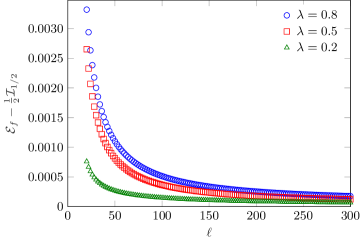
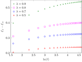
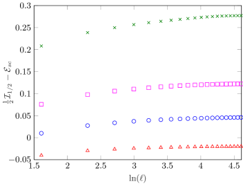
in the range up to $\ell=300$ and including also subleading corrections. A comparison of the fits for $c_{\mathrm{eff}}$ obtained from Eq. (26) and the analytic prediction (25) is shown on the left of Fig. 2, with a perfect agreement. Furthermore, we also compared the logarithmic negativity and the mutual information directly, with their difference shown on the right of Fig. 2. One can clearly see that the difference decreases with increasing $\ell$, which confirms the assumption $\mathcal{E}_{f}\simeq\frac{1}{2}\,\mathcal{I}_{1/2}$ up to subleading corrections that seem to vanish in the $\ell\to\infty$ limit.

IV Quench from equal fillings

After having investigated the ground-state problem, we now move to the quench scenario depicted in Fig. 1. First we consider equal fillings, restricting ourselves to the case of half-filled chains $n_{l}=n_{r}=1/2$. For a homogeneous chain ($\lambda=1$), the time evolution of the entanglement entropy after such a local quench has been calculated for hopping chains Eisler and Peschel (2007) as well as within CFT Calabrese and Cardy (2007); Stéphan and Dubail (2011). Moreover, CFT calculations could even be extended to the treatment of the negativity after the quench, using the techniques introduced in Calabrese et al. (2012b); Calabrese et al. (2013). For symmetric intervals in an infinite chain $N\to\infty$ and $t<\ell$, one obtains the result Wen et al. (2015)

$$\mathcal{E}_{f}=\frac{c}{4}\ln\left(\frac{t^{2}+\epsilon^{2}}{\epsilon^{2}}\frac{\ell-t}{\ell+t}\right)+\text{const},$$ (27)

where $\epsilon$ is a short-distance cutoff, ubiquitous in CFT calculations. Remarkably, the exact same result can be found for the Rényi mutual information $\frac{1}{2}\,\mathcal{I}_{1/2}$ in the limit of adjacent intervals, based on the the results of Ref. Asplund and Bernamonti (2014), where only the case $\alpha=1$ was considered but the generalization to $\alpha=1/2$ is trivial. It should be stressed that both CFT results contain, in general, a contribution from a non-universal function which, however, is expected to vanish for the Dirac fermion theory we are interested in, and is thus not included in (27). The characteristic feature of (27) is an early logarithmic growth for $t\ll\ell$ which then levels off into a plateau, followed by a sharp decrease around $t\to\ell$. For $t>\ell$, i.e. after the front created by the quench travels through the segment, the negativity assumes its ground-state value $\mathcal{E}_{f}=c/4\ln\ell+\mathrm{const}$.

On the other hand, for local quenches across a defect, another interesting result was found for the time evolution of the Rényi entropy of a half-chain, $\ell=N$. Namely, for a hopping chain with a defect, it turns out that the growth of the entropy is logarithmic and governed by the exact same effective central charge as found for the ground-state entanglement Eisler and Peschel (2012); Thomas and Flindt (2015). The result was later generalized to arbitrary CFTs with a conformal defect Wen et al. (2018). In particular, for $\alpha=1/2$ and in the limit $t\ll N$, one finds for the hopping chain

$$S_{1/2}(\rho_{A_{1}})=\frac{c_{\mathrm{eff}}}{2}\ln(t)+\mathrm{const},$$ (28)

where $c_{\mathrm{eff}}$ is given by (25). Note that in the homogeneous case $c_{\mathrm{eff}}=1$, and thus taking the limit $\ell\to\infty$, $t\gg\epsilon$ and setting $c=1$ in (27) exactly reproduces (28), as it should.

We now consider the negativity in the tripartite setup of Fig. 1. Similarly to the ground-state case in Sec. III, we argue that the relation $\mathcal{E}_{f}\simeq\frac{1}{2}\,\mathcal{I}_{1/2}$ should hold also for the local quench across a defect. However, apart from the homogeneous case $\lambda=1$, we are not aware of any calculations (neither lattice, nor CFT), which would generalize the formula (28) on the Rényi entropy for an interval $\ell<N$ that is not the half-chain. Nevertheless, it is reasonable to expect that, until the front reaches the boudary $t<\ell$, the entropy of the composite interval $S_{1/2}(\rho_{A})$ actually remains constant. Then, by combining the results (27) and (28), we propose the following simple ansatz

$$\mathcal{E}_{f}=\frac{c^{\prime}_{\mathrm{eff}}}{4}\ln\left(t^{2}\frac{\ell-t}{\ell+t}\right)+\text{const.}$$ (29)

Note that one has only two fitting parameters, namely the prefactor $c^{\prime}_{\mathrm{eff}}$ as well as the constant. Clearly, for the limiting cases $\lambda=0$ and $\lambda=1$, one has to have $c^{\prime}_{\mathrm{eff}}=0$ and $c^{\prime}_{\mathrm{eff}}=c=1$, respectively.

For intermediate values of $\lambda$, we have determined $c^{\prime}_{\mathrm{eff}}$ by fitting the ansatz (29) to the numerically calculated $\mathcal{E}_{f}$ curves for a fixed interval length $\ell=50$. The results are shown in Fig. 3. On the left of the figure the numerical data is shown together with the ansatz (29). On the right hand side we plot the obtained values of $c^{\prime}_{\mathrm{eff}}$ as a function of $\lambda$, compared to the equilibrium effective central charge $c_{\mathrm{eff}}$. One can clearly see that the two functions behave very similarly and one has $c^{\prime}_{\mathrm{eff}}\approx c_{\mathrm{eff}}$. Indeed, for larger values of $\lambda$ the agreement is almost perfect, however the deviation increases for smaller defect strengths. This is also obvious from the left of Fig. 3, where the data for $\lambda=0.2$ shows already some larger discrepancy compared to the fit function.

(a)

(b)

Figure 3: Left: time evolution of the logarithmic negativity $\mathcal{E}_{f}$ after a quench from equal fillings, for $\ell=50$ and $2N=600$. The red solid lines show the ansatz (29) the data is fitted to. Right: comparison of the fitted values of $c^{\prime}_{\mathrm{eff}}$ to the ground-state effective central charge $c_{\mathrm{eff}}$ from (25)

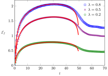
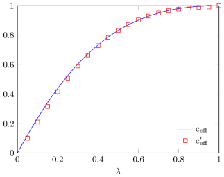
Although the mismatch of the data might be due to finite-size effects, we observe essentially the same behaviour for larger $\ell=75$. This rather suggests that the simplistic ansatz (29) is probably not the exact leading functional form of $\mathcal{E}_{f}$. In fact, we have also tried a more complicated three-parameter ansatz, assigning two different prefactors to the logarithmic terms with arguments $t$ and $(\ell-t)/(\ell+t)$. Unfortunately, however, the fits turn out to be very unstable against changing the fitting interval, making the results unreliable. Thus we conclude that, without some additional insights (e.g. from CFT calculations) on the structure of $\mathcal{E}_{f}$, extracting the proper time-dependece from numerical calculations is a very hard task.

We have also compared the behaviour of $\mathcal{E}_{f}$ and $\frac{1}{2}\,\mathcal{I}_{1/2}$ directly. One finds that the curves almost exactly overlap until roughly $t\approx\ell$, with no visible deviations. Around $t=\ell$ there is only a slight deviation between the two functions, which, however diminishes again for $t\gg\ell$. Indeed, both quantities are expected to converge towards their ground-state values asymptotically, where the deviation was already found to be tiny, see Fig. 2. Therefore, for better visibility of the data, we have not included $\frac{1}{2}\,\mathcal{I}_{1/2}$ in the left of Fig. 3.

V Quench from unequal fillings

We now study initial states with unequal fillings, where the behaviour of the entanglement negativity turns out to be qualitatively different from the unbiased case discussed above. In most of our calculations we shall actually consider the maximally biased case, $n_{l}=1$ and $n_{r}=0$, while at the end of the section we show that the generalization to arbitrary fillings is straightforward. Similarly to the unbiased case, we first discuss the negativity evolution for a homogeneous chain $(\lambda=1)$, where results can also be obtained via CFT techniques.

V.1 Homogeneous chain

This case is also known as the domain-wall quench, due to the form of the initial state in the spin-chain equivalent of the hopping model. Here one can work directly in the thermodynamic limit, $N\to\infty$, where the correlation matrix is known exactly and has the simple form Eisler and Rácz (2013)

$$C_{mn}(t)=\frac{i^{n-m}\,t}{2(m-n)}\left[J_{m-1}(t)J_{n}(t)-J_{m}(t)J_{n-1}(t)\right],$$ (30)

where $J_{m}(t)$ is the Bessel function of order $m$. Remarkably, the correlation matrix for the domain-wall quench is unitarily equivalent to the one in a static ground-state problem, namely a hopping chain with a linear chemical potential Eisler et al. (2009), with the time $t$ playing the role of the characteristic length scale of the potential. This can actually be shown to be a particular example of a more general mapping, known as emergent eigenstate solution Vidmar et al. (2017). Consequently, the entanglement properties in the dynamical and static problems are identical.

The entanglement entropy for a biased hopping chain was studied in Eisler et al. (2009); Eisler and Peschel (2014); Alba and Heidrich-Meisner (2014); Gruber and Eisler (2019) between two parts of the chain, with the cut located somewhere along the emerging front. The growth was found to be logarithmic, however with a different prefactor as for the local (unbiased) quench. The analytical understanding of the results for $n_{l}=1$ and $n_{r}=0$ came afterwards, when the method of curved-space CFT was developed Dubail et al. (2017). The basic idea is that certain inhomogeneous free-fermion problems can be treated by first mapping the problem to a CFT in a curved background metric. The entanglement entropies can be calculated by applying standard replica-trick methods Calabrese and Cardy (2009) for the curved-space Dirac fermion theory (see also Bastianello et al. for recent results on inhomogeneous Luttinger liquids). This makes it possible to extract the entropy analytically for a half-chain, or even generalize the calculations to a finite segment within the front region Dubail et al. (2017). The mutual information $\frac{1}{2}\,\mathcal{I}_{1/2}$ in our setup can be obtained immediately from the latter result.

Furthermore, it is possible to combine the curved-space technique with the CFT approach to the negativity Calabrese et al. (2012b); Calabrese et al. (2013). The calculation is straightforward but somewhat lengthy, thus we present it in Appendix B. As a result, we obtain for both the negativity and the mutual information

$$\mathcal{E}_{f}=\frac{1}{2}\,\mathcal{I}_{1/2}=\frac{1}{4}\ln\left[\,t\,f\left(\ell/t\right)\right]+c_{1},\qquad f(\xi)=\begin{cases}1&t<\ell\\ \frac{\left(1-\sqrt{1-\xi^{2}}\right)^{2}}{\xi^{3}}&t>\ell\end{cases}$$ (31)

Note that, apart from an explicit factor of $t$ which gives the logarithmic growth of the negativity, (31) depends only on a scaling function of the variable $\xi=\ell/t$. It should be stressed that the calculation in Appendix B refers only to $\xi<1$, as the curved-space CFT is able to describe only the front region with nontrivial fermionic density. However, the $\xi>1$ result can be obtained by using continuity and some simple arguments. Indeed, for $\ell>t$, the segments include parts of the chain outside the front, where the density is either zero or one. Clearly, these pieces do not contribute to the entanglement at all, which is thus given by the result for $\ell=t$, i.e. by the limit $\xi\to 1$.

The CFT results in (31) are compared to our numerical calculations in Fig. 4 with a very good agreement. The constant $c_{1}\approx 0.646$ has been obtained by fitting the data for $\mathcal{E}_{f}$ in the regime $t<\ell$. The only visible deviations are around $t=\ell$, i.e. when the boundaries of the segments are close to the edges of the front. Indeed, the front is known to have a nontrivial scaling behaviour around the edge Eisler and Rácz (2013); Viti et al. (2016); Fagotti (2017), characterized by the scale $t^{1/3}$, which is not resolved by the CFT treatment. Nevertheless, when plotted against $t/\ell=\xi^{-1}$ and after subtracting $1/4\ln(t)$, the lattice data for increasing $\ell$ converge smoothly towards the CFT result as shown in the inset of Fig. 4. Note also that the $t\to\infty$ behaviour can be obtained by expanding $f(\xi)\approx\xi$/4 for $\xi\to 0$, such that the steady state is characterized by $\mathcal{E}_{f}=1/4\ln\ell+\mathrm{const}$.

Figure 4: Logarithmic negativity $\mathcal{E}_{f}$ and mutual information $\frac{1}{2}\,\mathcal{I}_{1/2}$ after the domain wall quench in a homogeneous chain ($\lambda=1$), compared to the CFT prediction (31) (red solid lines) for two different segment sizes. The inset shows the scaled data around $t=\ell$, after substracting $\frac{1}{4}\ln(t)$.

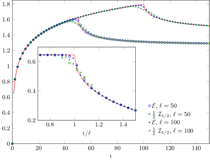
V.2 Chain with a defect

The time evolution of entanglement across a defect turns out to be qualitatively different Eisler and Peschel (2012). Indeed, an imperfect transmission between the half-chains gives rise to scattering, i.e. the single-particle modes are partially transmitted and reflected with probabilities $T_{q}$ and $R_{q}=1-T_{q}$, respectively. For a weak hopping defect parametrized by $\lambda=\mathrm{e}^{-\nu}$, the transmission coefficient is given by

$$T_{q}=\frac{\sin^{2}(q)}{\cosh^{2}(\nu)-\cos^{2}(q)}\,.$$ (32)

The transmitted and reflected particles become entangled in the wavefunction, and the contribution of such a pair in the $\alpha=1/2$ Rényi entropy is $s_{1/2}(T_{q})$, where

$$s_{1/2}(x)=2\ln\left(x^{1/2}+(1-x)^{1/2}\right)$$ (33)

is the density of the Rényi entropy, c.f. Eq. (11). Now, due to the density bias in the initial state, there is a constant influx of particles and consequently a steady generation of entanglement at the defect. For a half-chain, $\ell=N$, at maximum bias and in the limit $N\to\infty$, this was found to give, to leading order, a linear growth of entanglement Eisler and Peschel (2012)

$$S_{1/2}(\rho_{A_{1}})=t\int_{0}^{\pi}\frac{\mathrm{d}q}{2\pi}\,v_{q}\,s_{1/2}(T_{q})\,,$$ (34)

where $v_{q}=\sin(q)$ is the single-particle group velocity and the integral is taken over all modes with $v_{q}>0$.

This simple semiclassical picture of entanglement production, based on the propagation of entangled pairs of quasiparticles, bears a strong similarity to global quenches Calabrese and Cardy (2005); Alba and Calabrese (2017). One should stress, however, that here the pairs are created solely at the defect site but steadily in time, in contrast to a global quench where pairs are created only at $t=0$ but homogeneously along the chain. Nevertheless, the continuity argument $\mathcal{E}_{f}\simeq\frac{1}{2}\,\mathcal{I}_{1/2}$ can be applied the very same way as for the global quench Alba and Calabrese (2019). Indeed, due to the strictly local production of entanglement at the common boundary of the segments, the only effect of their finite size is to cut off the growth of the negativity once the distance travelled by a given mode $v_{q}t$ exceeds the segment size $\ell$. This leads to the semiclassical expression

$$\mathcal{E}_{sc}=\int_{0}^{\pi}\frac{\mathrm{d}q}{2\pi}\min{(v_{q}t,\ell)}\,s_{1/2}(T_{q})\,.$$ (35)

To test the validity of our ansatz $\mathcal{E}_{sc}$, in Fig. 5 we plot the integrals (35) for various $\lambda$ and compare them to the numerical data for $\mathcal{E}_{f}$ and $\frac{1}{2}\,\mathcal{I}_{1/2}$ obtained for a chain of length $2N=500$ from the correlation-matrix method. One can see that the semiclassical picture provides a rather good description of the data to leading order, there are, however, still some sizeable corrections which tend to diminish for smaller values of $\lambda$. The quantities $\mathcal{E}_{f}$ and $\frac{1}{2}\,\mathcal{I}_{1/2}$ perfectly overlap in the regime $t<\ell$ of linear growth, where the result is identical to the one for the half-chain (34), as there is no contribution to the entanglement from the outer boundaries of the segments. Interestingly, however, there is a clearly visible splitting for $t>\ell$, after the front has traversed the segments.

Figure 5: Entanglement negativity $\mathcal{E}_{f}$ (circles) and mutual information $\frac{1}{2}\,\mathcal{I}_{1/2}$ (squares) after a quench from unequal fillings $n_{l}=1$ and $n_{r}=0$, compared to the semiclassical ansatz (35) (lines) for $\ell=40$ and different values of $\lambda$.

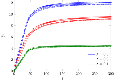
In order to better understand the corrections beyond the semiclassical picture, in Fig. 6 we have subtracted $\mathcal{E}_{sc}$ from the data, shown for the two larger values of $\lambda$ and several segment sizes. Similarly to $\mathcal{E}_{sc}$, the deviation also shows different behaviour in the regimes $t<\ell$ and $t>\ell$. Until roughly $t\approx\ell$, one observes a steady growth which becomes slower for larger defect strengths. A closer inspection shows that this subleading growth is actually slower than logarithmic for all the values $\lambda\neq 1$ we have checked. When the front crosses the segment boundary, one has a sharp drop in all of the curves, which is then followed again by a very slow increase. Note that the splitting of the $\mathcal{E}_{f}$ and $\frac{1}{2}\,\mathcal{I}_{1/2}$ curves is even more apparent in Fig. 6. However, due to the very slow variation of the data, it is hard to draw a firm conclusion about the asymptotic behaviour, despite the relatively large times considered in the calculations.

(a)

(b)

Figure 6: Deviations of $\mathcal{E}_{f}$ (solid lines) and $\frac{1}{2}\,\mathcal{I}_{1/2}$ (dashed lines) from the semiclassical ansatz (35) for $\lambda=0.8$ (left) and $\lambda=0.5$ (right) and various segment sizes $\ell$.

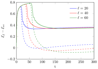
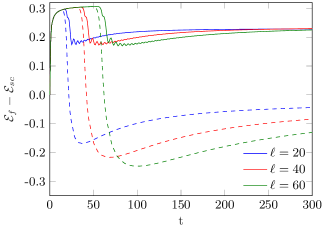
The steady state after the quench across the defect can actually be captured directly. Indeed, the elements of the correlation matrix in (5) have a well defined limit Ljubotina et al. (2019)

$$\tilde{C}_{m,n}=\lim_{t\to\infty}\lim_{N\to\infty}C_{m,n}(t)\,,$$ (36)

with the explicit formulas collected in Appendix A. These can be used to evaluate the subleading scaling of the steady-state negativity and mutual information, i.e. after subtracting the extensive contribution $\lim_{t\to\infty}\mathcal{E}_{sc}$ that follows from the semiclassical description (35). The results are shown in Fig. 7, with both the data for $\mathcal{E}_{f}$ (left) as well as $\frac{1}{2}\,\mathcal{I}_{1/2}$ (right) plotted against $\ln(\ell)$. Rather clearly, the subleading terms in the steady state are different for the two quantities and the scaling in $\ell$ is slower than logarithmic. This is also supported by the form of the steady-state correlation matrix (61) on a given side of the defect, which is a Toeplitz matrix with a symbol given by $T_{q}$ for $q>0$ and zero otherwise. While this yields immediately the extensive part of the negativity (35), one has also $T_{q}\to 0$ for $q\to 0$ and thus no jump singularity is present. Nevertheless, the symbol is still nonanalytic and shows a very sharp increase around $q=0$ as $\lambda\to 1$. Thus a weaker than logarithmic growth of the subleading term, although unlikely from the numerics, cannot be excluded.

(a)

(b)

Figure 7: Steady-state negativity (left) and mutual information (right), as calculated from the correlation matrix (36) after subtracting the extensive semiclassical contribution (35). The data is plotted against $\ln(\ell)$ for various defect strengths $\lambda$. Note the different vertical scales.

Finally, we briefly consider the case of arbitrary fillings with $n_{l}>n_{r}$. The straightforward generalization of the semiclassical ansatz reads

$$\mathcal{E}_{sc}=\int\displaylimits_{q_{F,r}}^{q_{F,l}}\frac{\mathrm{d}q}{2\pi}\min{(v_{q}t,\ell)}\,s_{1/2}(T_{q})\,,$$ (37)

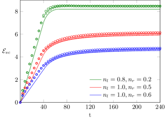
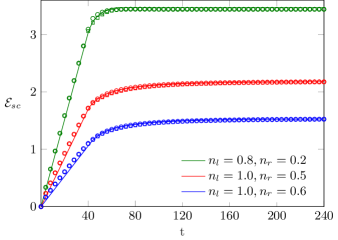
where the integral is carried out only between the Fermi wavenumbers $q_{F,\sigma}=\pi n_{\sigma}$. In other words, one has to consider only the contributions from the uncompensated fermionic modes, that can propagate from the left to the right half-chain. The resulting curves are shown in Fig. 8, for two different $\lambda$ and various fillings, together with the numerically calculated $\mathcal{E}_{f}$ and $\frac{1}{2}\,\mathcal{I}_{1/2}$ in a chain of size $2N=500$. As expected, the plots are very similar to the one in Fig. 5, with the deviations from the semiclassical prediction decreasing for smaller $\lambda$. Due to the similar qualitative behaviour, a detailed analysis of the subleading terms is not presented for this case.

(a)

(b)

Figure 8: Entanglement negativity $\mathcal{E}_{f}$ (circles) and mutual information $\frac{1}{2}\,\mathcal{I}_{1/2}$ (squares) after a quench from various unequal fillings, compared to the semiclassical ansatz (37) (lines) for $\ell=40$ and $\lambda=0.5$ (left) resp. $\lambda=0.1$ (right).

VI Quench in the XXZ chain with a defect

Finally we are considering a quench in the XXZ spin chain, given by the Hamiltonian

$$\hat{H}_{XXZ}=\sum_{j=-N+1}^{N-1}\left[J_{j}\left(S_{j}^{x}S_{j+1}^{x}+S_{j}^{y}S_{j+1}^{y}\right)+\Delta S_{j}^{z}S_{j+1}^{z}\right],$$ (38)

where $S_{j}^{\alpha}$ are spin-$1/2$ operators, $\Delta$ is the anisotropy parameter, and the XX-coupling is given by

$$J_{j}=\begin{cases}1&\text{if}\ j\neq 0\,,\\ \lambda\,\Theta(t)&\text{if}\ j=0\,.\end{cases}$$ (39)

Here $\Theta(t)$ is the Heaviside step function, in other words, the quench consists of simply joining two decoupled XXZ half-chains at time $t=0$. Applying a Jordan-Wigner transformation, the Hamiltonian (38) can be mapped into a chain of interacting fermions and the setup becomes exactly the same as the one depicted in Fig. 1 for free fermions without a density bias.

However, it turns out that the negativity depends on the choice of basis and is not equivalent in the fermion or spin representation. Indeed, using spin variables, one has to apply the conventional definition of the logarithmic negativity via the partial transpose of the density matrix Vidal and Werner (2002)

$$\mathcal{E}_{s}=\ln\|\rho_{A}^{T_{2}}\|_{1}\,.$$ (40)

Here the partial transpose is taken with respect to subsystem $A_{2}$, defined by its matrix elements as

$$\bra{e^{(1)}_{i},e^{(2)}_{j}}\rho_{A}^{T_{2}}\ket{e^{(1)}_{k},e^{(2)}_{l}}=\bra{e^{(1)}_{i},e^{(2)}_{l}}\rho_{A}\ket{e^{(1)}_{k},e^{(2)}_{j}},$$ (41)

where $\ket{e^{(1)}_{i}}$ and $\ket{e^{(2)}_{j}}$ denote orthonormal bases on the Hilbert spaces pertaining to segments $A_{1}$ and $A_{2}$.

Clearly, since we are now faced with a non-Gaussian problem, we have to compute the negativity $\mathcal{E}_{s}$ via density-matrix renormalization group (DMRG) Schollwöck (2011); White (1992, 1993) methods. In particular, the time evolution $\ket{\psi(t)}=e^{-i\hat{H}_{XXZ}t}\ket{\psi(0)}$ after the quench is first performed with time-dependent DMRG (tDMRG) simulations Daley et al. (2004); White and Feiguin (2004), which give access to the reduced density matrix $\rho_{A}$ in a matrix product state (MPS) representation ite . The partial transpose and the corresponding logarithmic negativity can then be calculated using the method of Ref. Ruggiero et al. (2016), which is briefly reviewed in the following subsection.

VI.1 Negativity for matrix product states

Let us consider the time-evolved state after the quench $\ket{\psi(t)}=e^{-i\hat{H}_{XXZ}t}\ket{\psi(0)}$ and its MPS representation

$$\ket{\psi(t)}=\sum_{\sigma_{1}\dots\sigma_{2N}}T_{\nu_{1}}^{\sigma_{1}}T_{\nu_{1}\nu_{2}}^{\sigma_{2}}\dots T_{\nu_{2N-1}}^{\sigma_{2N}}\ket{\sigma_{1}\dots\sigma_{2N}},$$ (42)

where $T_{\nu_{i-1}\nu_{i}}^{\sigma_{i}}$ denotes the tensor on site $i$ with bond indices $\nu_{i-1}$ and $\nu_{i}$ and the physical index $\sigma_{i}=0,1$. In Eq. (42) and all the following equations, we assume summation over all repeated bond indices $\nu_{i}$ implicitly, and indicate only summations over the physical indices for better readability.

Our goal is to calculate the negativity for the geometry depicted in Fig. 1, i.e. between two adjacent segments $A_{1}$ and $A_{2}$ with $A=A_{1}\cup A_{2}$. The main step is to construct the reduced density matrix $\rho_{A}$, which is shown graphically on the left of Fig. 9, after tracing out over the environment $B$. The squares in different colors depict the tensors belonging to either subsystems $A_{1}$ or $A_{2}$, c.f. Fig. 1. One can now introduce new basis states in the Hilbert spaces of the two intervals $A_{1}$ and $A_{2}$ as

$$\ket{w^{(1)}_{\nu_{1l},\nu_{1r}}}=\sum_{\{\sigma_{i}\}}\prod_{i\in A_{1}}T_{\nu_{i-1}\nu_{i}}^{\sigma_{i}}\ket{\sigma_{i}},\qquad\ket{w^{(2)}_{\nu_{2l},\nu_{2r}}}=\sum_{\{\sigma_{i}\}}\prod_{i\in A_{2}}T_{\nu_{i-1}\nu_{i}}^{\sigma_{i}}\ket{\sigma_{i}},$$ (43)

where the index pairs $\nu_{1l},\nu_{1r}$ and $\nu_{2l},\nu_{2r}$ indicate the uncontracted left- and rightmost bond indices for each block. Using these basis states, we can eventually write the reduced density matrix as

$$\rho_{A}=\delta_{\nu_{1l},\nu^{\prime}_{1l}}\delta_{\nu_{2r},\nu^{\prime}_{2r}}\delta_{\nu_{1r},\nu_{2l}}\delta_{\nu^{\prime}_{1r},\nu^{\prime}_{2l}}\ket{w^{(1)}_{\nu_{1l},\nu_{1r}}}\bra{w^{(1)}_{\nu^{\prime}_{1l},\nu^{\prime}_{1r}}}\otimes\ket{w^{(2)}_{\nu_{2l},\nu_{2r}}}\bra{w^{(2)}_{\nu^{\prime}_{2l},\nu^{\prime}_{2r}}},$$ (44)

where the delta functions carry out the contractions of the remaining bond indices, as visualized in the left of Fig. 9.

Figure 9: Graphical representation of the reduced density matrix $\rho_{A}$ (left), the transfer matrix $E_{1}$ corresponding to the segment $A_{1}$ (middle), and its singular value decomposition (right). The boxes represent tensors with the contractions indicated by the links between them.

The representation (44) yields a decomposition of $\rho_{A}$ on the two subspaces corresponding to $A_{1}$ and $A_{2}$. However, the main problem is that the choice of basis in (43) is not orthogonal. Indeed, the overlaps between these states are given by the so-called transfer matrices

$$\braket{w^{(1)}_{\nu_{1l},\nu_{1r}}}{w^{(1)}_{\nu^{\prime}_{1l},\nu^{\prime}_{1r}}}=\left[E_{1}\right]^{\nu_{1l},\nu_{1r}}_{\nu^{\prime}_{1l},\nu^{\prime}_{1r}},\qquad{\braket{w^{(2)}_{\nu_{2l},\nu_{2r}}}{w^{(2)}_{\nu^{\prime}_{2l},\nu^{\prime}_{2r}}}}=\left[E_{2}\right]^{\nu_{2l},\nu_{2r}}_{\nu^{\prime}_{2l},\nu^{\prime}_{2r}},$$ (45)

that are obtained by contracting all the tensors with their complex conjugates via their physical indices within the respective segment

$$\left[E_{1}\right]^{\nu_{1l},\nu_{1r}}_{\nu^{\prime}_{1l},\nu^{\prime}_{1r}}=\prod_{i\in A_{1}}\sum_{\sigma_{i}}T_{\nu_{i-1}\nu_{i}}^{\sigma_{i}}\bar{T}_{\nu^{\prime}_{i-1}\nu^{\prime}_{i}}^{\sigma_{i}}\,,\qquad\left[E_{2}\right]^{\nu_{2l},\nu_{2r}}_{\nu^{\prime}_{2l},\nu^{\prime}_{2r}}=\prod_{i\in A_{2}}\sum_{\sigma_{i}}T_{\nu_{i-1}\nu_{i}}^{\sigma_{i}}\bar{T}_{\nu^{\prime}_{i-1}\nu^{\prime}_{i}}^{\sigma_{i}}\,.$$ (46)

These objects are thus four-index tensors, corresponding to the uncontracted left- and rightmost bond indices, see the middle panel of Fig. 9 for a graphical representation of $E_{1}$.

In order to obtain an orthogonal basis, one has to perform a singular value decomposition (SVD) of the transfer matrices $E_{1}=U_{1}D_{1}V_{1}^{\dagger}$ and $E_{2}=U_{2}D_{2}V_{2}^{\dagger}$. This amounts to introducing a basis change via

$$\ket{w^{(1)}_{\nu_{1l},\nu_{1r}}}=\sum_{m}\left[N_{1}\right]^{m}_{\nu_{1l},\nu_{1r}}\ket{v_{m}^{(1)}},\qquad\ket{w^{(2)}_{\nu_{2l},\nu_{2r}}}=\sum_{n}\left[N_{2}\right]^{n}_{\nu_{2l},\nu_{2r}}\ket{v_{n}^{(2)}},$$ (47)

where $N_{1}=U_{1}D_{1}^{1/2}$ and $N_{2}=U_{2}D_{2}^{1/2}$, and the new indices $m$ and $n$ correspond to the singular values contained in the diagonal matrices $D_{1}$ and $D_{2}$. The pictorial representation of the SVD for $E_{1}$ is shown on the right of Fig. 9, where $D_{1}^{1/2}$ is depicted by the green rhombi. Inserting (47) into (44), one immediately obtains the matrix elements of the reduced density matrix

$$\left[\rho_{A}\right]^{m,m^{\prime}}_{n,n^{\prime}}=\left[N_{1}\right]^{m}_{\nu_{1l},\nu_{2l}}\left[\bar{N}_{1}\right]^{m^{\prime}}_{\nu_{1l},\nu^{\prime}_{2l}}\left[N_{2}\right]^{n}_{\nu_{2l},\nu_{2r}}\left[\bar{N}_{2}\right]^{n^{\prime}}_{\nu^{\prime}_{2l},\nu_{2r}}$$ (48)

expressed in the orthogonal bases $\ket{v_{m}^{(1)}}$ and $\ket{v_{n}^{(2)}}$. Note that (48) is now exactly in the form required to carry out the partial transposition according to (41). Indeed, the index pairs $m,m^{\prime}$ and $n,n^{\prime}$ correspond to the intervals $A_{1}$ and $A_{2}$, respectively. Therefore, the matrix elements of $\rho^{T_{2}}_{A}$ can simply be obtained by exchanging $n$ and $n^{\prime}$. Finally, the logarithmic negativity $\mathcal{E}_{s}$ in Eq. 40 can be calculated via an explicit diagonalization of $\rho^{T_{2}}_{A}$.

Regarding the computational effort, one has to stress that the cost of constructing the transfer matrices in (46) scales as $\mathcal{O}(\chi_{max}^{6})$ with the maximum bond dimension $\chi_{max}$ of the MPS. This, however, grows with the time evolution where we set the requirement $\epsilon\sim 10^{-8}-10^{-9}$ for the truncated weight. For a feasible computation of the transfer matrices, we truncated back the bond dimension to $\chi_{max}=300$. The range of each index $m,m^{\prime}$ as well as $n,n^{\prime}$ in the representation (48) is then bounded by $\chi^{2}_{max}$, which is still too large for a tractable calculation. However, since the singular values of $E_{1}$ and $E_{2}$ decay rapidly, one can apply a truncation after the SVD which we set to $\chi^{\prime}_{max}=80$. All in all, the evaluation of entanglement negativity is computationally much more demanding than that of the entropy, severely limiting the attainable segment sizes and simulation times in our numerics.

VI.2 Numerical results

The methods outlined in the previous subsection are now used to evaluate the time evolution of the logarithmic negativity across a defect in the XXZ chain. We focus exclusively on the unbiased case, as the bias induces a much more rapid growth of entanglement, which makes the DMRG calculations very demanding. We first present the results for the XX chain, which is just the special case of $\Delta=0$ in (38). Note that, even though the XX chain with a defect is exactly mapped into the fermionic Hamiltonian in Eq. (1) via a Jordan-Wigner transformation, the negativity $\mathcal{E}_{s}$ calculated for the spin chain in (40) is not equivalent to the fermionic one $\mathcal{E}_{f}$ defined in (15). Indeed, it has been shown in Eisler and Zimborás (2015) that the partial transposition in the spin basis yields a linear combination of two fermionic Gaussian operators

$$\rho_{A}^{T_{2}}=\frac{1-i}{2}O_{+}+\frac{1+i}{2}O_{-}\,,$$ (49)

where $O_{+}=\rho_{A}^{R_{2}}$ is the operator obtained in (14) by partial time reversal of the fermionic degrees of freedom and $O_{-}=O_{+}^{\dagger}$. Since in general the operators $O_{+}$ and $O_{-}$ do not commute, one has no access to the spectrum of $\rho_{A}^{T_{2}}$ and hence to $\mathcal{E}_{s}$ via simple covariance-matrix techniques. Nevertheless, the spin-chain negativity can be shown to be upper-bounded by the fermionic one as Herzog and Wang (2016); Eisert et al. (2018)

$$\mathcal{E}_{s}\leq\mathcal{E}_{f}+\ln\sqrt{2}\,.$$ (50)

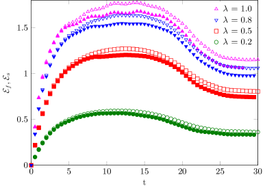
The time evolution of $\mathcal{E}_{s}$ obtained from tDMRG simulations are shown by the full symbols in Fig. 10 for various defect strengths $\lambda$. The results are compared to the fermionic negativity $\mathcal{E}_{f}$, shown by the empty symbols, and indicate that the upper bound in (50) actually holds even without the additional constant, i.e. one has $\mathcal{E}_{s}\leq\mathcal{E}_{f}$. The two quantities have a very similar qualitative behaviour, with their difference diminishing with decreasing $\lambda$. Unfortunately, however, the simulation times as well as the size of the segments are severely limited in the tDMRG simulations due to the increasing entanglement and bond dimension during time evolution, especially for higher values of $\lambda$. This makes a quantitative analysis of the discrepancy between $\mathcal{E}_{s}$ and $\mathcal{E}_{f}$ rather complicated.

Figure 10: Time evolution of the entanglement negativity $\mathcal{E}_{s}$ (full symbols) for two adjacent segments of size $\ell=20$ across a defect of various strengths $\lambda$ in an XX chain with $2N=100$. The data for the fermionic negativity $\mathcal{E}_{f}$ (empty symbols) in the analogous quench of the hopping chain with a defect is shown for comparison.

We also performed analogous tDMRG simulations for the XXZ chain with the anisotropy parameter $0<\Delta<1$. The fermionic analogue of this setting corresponds to an interacting problem and thus not amenable to Gaussian techniques. We first considered the homogeneous case $\lambda=1$, where the post-quench Hamiltonian is integrable and its low-energy behaviour is described by a Luttinger liquid. In particular, the spreading of excitations created above the ground state is given by the spinon velocity Franchini (2017)

$$v_{s}=\frac{\pi}{2}\frac{\sqrt{1-\Delta^{2}}}{\arccos{(}\Delta)}\,.$$ (51)

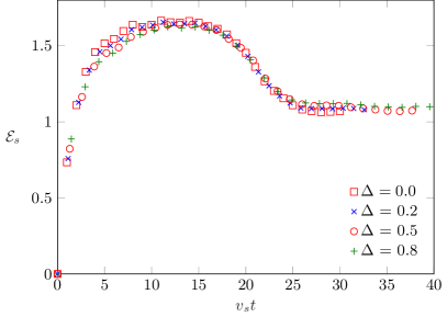
This strongly suggests that the main difference with respect to the homogeneous XX quench is due to the change in the Fermi velocity. On the left of Fig. 11 we have thus plotted the logarithmic negativity $\mathcal{E}_{s}$ calculated for various $\Delta$ against the variable $v_{s}t$, which indeed leads to a nice data collapse.

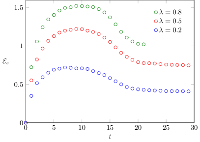
The situation for $\lambda\neq 1$ is more complicated, as the presence of the defect breaks the integrability of the model. The time evolution of the negativity is shown on the right of Fig. 11 for various defect strengths $\lambda$ and fixed $\Delta=0.5$, for a segment size $\ell=20$. Qualitatively, one observes a very similar behaviour as for the XX chain in Fig. 10. However, in previous studies of the half-chain entropy in Ref. Collura and Calabrese (2013) it was observed that the entropy growth is actually suppressed for repulsive interactions $\Delta>0$, corresponding to an effective central charge that goes to zero in the limit of large chain sizes. This is actually the same mechanism that was found for the ground-state entropy of the XXZ chain with a defect Zhao et al. (2006), and is the manifestation of a Kane-Fisher type renormalization behaviour Kane and Fisher (1992). Therefore it is reasonable to expect that the entanglement negativity would show a similar behaviour in the limit of large $\ell$. Unfortunately, however, the segment sizes required to test such a crossover are well beyond the limitations of our simulations.

Figure 11: Time evolution of the entanglement negativity $\mathcal{E}_{s}$ for two adjacent segments of size $\ell=20$ in an XXZ chain with $2N=100$. Left: homogeneous quench ($\lambda=1$) for different anisotropies $\Delta$. Right: quench across a defect of different strengths $\lambda$ and $\Delta=0.5$.

VII Discussion

We have studied entanglement in a hopping chain with a defect, focusing on the fermionic version of the logarithmic negativity $\mathcal{E}_{f}$ between two segments neighbouring the defect, and its relation to the Rényi mutual information $\frac{1}{2}\,\mathcal{I}_{1/2}$. In the ground state of the chain, the negativity scales logarithmically with an effective central charge $c_{\mathrm{eff}}$, and the difference $\mathcal{E}_{f}-\frac{1}{2}\,\mathcal{I}_{1/2}$ goes to zero for increasing segment sizes. For a quench across the defect, starting from disconnected half-chains both at half filling, the growth of the negativity is logarithmic in time and the prefactor seems to be well approximated by $c_{\mathrm{eff}}$. When the quench is performed from biased fillings, the entanglement growth becomes linear, followed by a saturation at an extensive value, which is due to backscattering from the defect and can be understood in a semiclassical picture. Although the ansatz (35) gives a very good leading order description of both $\mathcal{E}_{f}$ and $\frac{1}{2}\,\mathcal{I}_{1/2}$, the subleading corrections behave differently and their difference in the steady state remains finite even for large segment sizes. We have also calculated the standard logarithmic negativity $\mathcal{E}_{s}$ via DMRG methods in the XXZ spin chain after a (unbiased) quench across a defect. In the noninteracting XX case, closely related to the fermionic chain, we found that the spin-chain negativity is upper bounded by the fermionic one, $\mathcal{E}_{s}\leq\mathcal{E}_{f}$. In the general XXZ case, the results for $\mathcal{E}_{s}$ look qualitatively similar to the XX case for the small segment sizes attainable.

While the entanglement growth in the biased case has a very clear physical interpretation, the result for equal fillings is harder to grasp and would require some insight from CFT calculations. In fact, for the bipartite case of a half-chain, the CFT representation of the density matrix after the quench can be transformed into the one for the ground state by an appropriate conformal mapping Wen et al. (2018). Unfortunately, however, this transformation works only for the half-chain and it is unclear whether a generalization to our geometry exists.

It is important to stress that, although the semiclassical picture for unequal fillings is analogous to the one for a global quench Alba and Calabrese (2019), the qualitative behaviour of the negativity is completely different. Indeed, in the latter case the quasiparticles are created only at $t=0$, and thus the pairs that contribute to the entanglement growth eventually leave the segments. This implies that the negativity will decrease again for large times, decaying towards zero. In contrast, in our case there is a constant production of entangled pairs at the defect, and thus the negativity keeps growing until it eventually saturates at an extensive value. Furthermore, while for the global quench the deviation between $\mathcal{E}_{f}$ and $\frac{1}{2}\,\mathcal{I}_{1/2}$ seems to vanish for increasing $\ell$, for the defect we observe a finite difference between the two quantities. Understanding the origin of this discrepancy requires further investigations.

Finally, it would be interesting to extend these investigations to disjoint segments. In particular, it would be illuminating to see how the disagreement between the fermionic and XX chain negativities changes with separation. One expects the discrepancy to become larger, as the partial transpose is a sum of four fermionic Gaussian operators already in the ground state Coser et al. (2015). While the extension of both the fermionic as well as the spin-chain calculations are, in principle, straightforward, the computational effort of the DMRG calculations are much more demanding and are thus left for future studies.

Appendix A Correlation matrices for the defect

We collect here the integral formulas for the correlation matrix elements $\braket{c^{\dagger}_{m}c_{n}}$ in the thermodynamic limit $N\to\infty$ of the hopping chain (1), with a single weak hopping defect parametrized by $\lambda=\mathrm{e}^{-\nu}$. We consider both the ground state of the chain as well as the NESS after time evolution from a domain wall. The former has been considered in Ref. Peschel (2005) while in the latter case the results were obtained in Ref. Ljubotina et al. (2019). In each case the result depends on whether the lattice sites are chosen on the same (left or right) or opposite sides of the defect, i.e. the correlation matrix has a block form. We shall only consider matrix elements with $m\leq n$, since the others follow from hermiticity.

In the ground state of an infinite chain, the matrix elements read

$$C_{m,n}=\begin{cases}C_{0}(n-m)-C_{1}(n+m)&\mbox{if $m,n\geq 1$}\\ C_{0}(n-m)-C_{1}(2-n-m)&\mbox{if $m,n\leq 0$}\\ C_{2}(n-m)&\mbox{if $m\leq 0$, $n\geq 1$}\end{cases}$$ (52)

where the different contributions depend only on the difference $r=n-m$ and sum $s=n+m$ of the indices. The first translationally invariant piece is given by

$$C_{0}(r)=\frac{\sin(\frac{\pi}{2}r)}{\pi r}\,,$$ (53)

which is just the homogeneous result. The extra contributions on the same side of the defect were obtained in Peschel (2005) and read

$$C_{1}(s)=\frac{\mathrm{sh}\,\nu}{2}(\mathrm{e}^{\nu}I_{s}-\mathrm{e}^{-\nu}I_{s-2}),$$ (54)

where

$$I_{s}=\int_{0}^{\pi/2}\frac{\mathrm{d}q}{\pi}\frac{\cos qs}{\mathrm{sh}^{2}\,\nu+\sin^{2}q}\,.$$ (55)

Interestingly, one observes that the contributions $C_{1}(2k)=0$ vanish completely for even $s=2k$, which follows from the property $\mathrm{e}^{\nu}I_{2k}=\mathrm{e}^{-\nu}I_{2k-2}$ of the integrals defined above. Finally, the matrix elements on opposite sides of the defect are given by

$$C_{2}(r)=\frac{\mathrm{ch}\,\nu}{2}I_{r}-\frac{\mathrm{e}^{\nu}}{4}I_{r+2}-\frac{\mathrm{e}^{-\nu}}{4}I_{r-2}\,.$$ (56)

Using the property found above, it is easy to see that also these contributions vanish for $r=2k$. Thus the correlation matrix has a checkerboard structure as in the homogeneous case.

In the limit $\nu=0$ one has trivially $C_{1}(s)=0$, whereas for the offdiagonal block one finds

$$C_{2}(r)=\int_{0}^{\pi/2}\frac{\mathrm{d}q}{2\pi}\frac{\cos qr-\left[\cos q(r-2)+\cos q(r+2)\right]/2}{\sin^{2}q}=\int_{0}^{\pi/2}\frac{\mathrm{d}q}{\pi}\cos qr=C_{0}(r)\,,$$ (57)

i.e. one recovers the results for the homogeneous chain. In the opposite limit $\nu\to\infty$ of a vanishing defect coupling, one finds $C_{1}(s)=C_{0}(s)$ which is the result for a half-infinite chain. On the other hand, $C_{2}(r)=0$ as it should for two decoupled half-chains.

Now we consider the correlation matrix elements $\tilde{C}_{m,n}$ for the NESS, which emerges in the $t\to\infty$ limit of time evolution from a domain wall initial state. The results were obtained in Ljubotina et al. (2019) by solving the problem for a finite system size and time and then considering the limits $N\to\infty$ and $t\to\infty$ via contour integration tricks. In order to bring the formulas for the matrix elements in a transparent form, it is useful to introduce the transmission and reflection coefficients

$$T_{q}=\frac{\sin^{2}q}{\mathrm{sh}^{2}\,\nu+\sin^{2}q}\,,\qquad R_{q}=\frac{\mathrm{sh}^{2}\,\nu}{\mathrm{sh}^{2}\,\nu+\sin^{2}q}\,,$$ (58)

as well as the auxiliary integral expressions

$$\tilde{I}_{r}=\int_{0}^{\pi}\frac{\mathrm{d}q}{2\pi}\frac{i\,\sin qr}{\mathrm{sh}^{2}\,\nu+\sin^{2}q}\,.$$ (59)

Analogously to (52), the matrix elements can be written down by a separation of cases

$$\tilde{C}_{m,n}=\begin{cases}\tilde{C}_{0}(n-m)&\mbox{if $m,n\geq 1$}\\ \delta_{m,n}-\tilde{C}_{0}(m-n)&\mbox{if $m,n\leq 0$}\\ \tilde{C}_{2}(n-m)+\tilde{C}_{3}(n+m)&\mbox{if $m\leq 0$, $n\geq 1$}\end{cases}$$ (60)

The correlations are thus translationally invariant if both sites are located on the same side. They can be written in a very instructive form

$$\tilde{C}_{0}(r)=\int_{0}^{\pi}\frac{\mathrm{d}q}{2\pi}T_{q}\,\mathrm{e}^{iqr}.$$ (61)

Indeed, this can be interpreted as a correlation matrix where the occupation function is given by the transmission probability for all the modes with positive velocities. Note that the correlations on the left/right hand side are now related by the symmetry property $\tilde{C}_{m,n}=\delta_{m,n}-\tilde{C}_{1-m,1-n}$. If the sites are located on opposite sides, the correlations are given via the expressions

$$\tilde{C}_{2}(r)=\frac{\mathrm{ch}\,\nu}{2}\tilde{I}_{r}-\frac{\mathrm{e}^{\nu}}{4}\tilde{I}_{r+2}-\frac{\mathrm{e}^{-\nu}}{4}\tilde{I}_{r-2}\,$$ (62)

and

$$\tilde{C}_{3}(s)=i\int_{0}^{\pi}\frac{\mathrm{d}q}{2\pi}\sqrt{T_{q}R_{q}}\,\mathrm{e}^{iq(s-1)}\,.$$ (63)

The limiting cases are also straightforward to obtain. For $\nu=0$ we have $T_{q}\equiv 1$ and $R_{q}\equiv 0$ such that

$$\tilde{C}_{0}(r)=\frac{1}{2}\delta_{r,0}+i\int_{0}^{\pi}\frac{\mathrm{d}q}{2\pi}\sin qr\,,$$ (64)

which is exactly the NESS result for the homogeneous chain. For the offdiagonal block one obtains $C_{3}(s)=0$ as well as

$$\tilde{C}_{2}(r)=i\int_{0}^{\pi}\frac{\mathrm{d}q}{4\pi}\frac{\sin qr-\left[\sin q(r-2)+\sin q(r+2)\right]/2}{\sin^{2}q}=i\int_{0}^{\pi}\frac{\mathrm{d}q}{2\pi}\sin qr\,,$$ (65)

i.e. the full matrix becomes translationally invariant, as it should. In the opposite limit $\nu\to\infty$ one has $T_{q}\equiv 0$ and $R_{q}\equiv 1$, and thus $\tilde{C}_{0}(r)=\tilde{C}_{2}(r)=\tilde{C}_{3}(s)=0$. One then simply recovers the initial $t=0$ form of the correlation matrix since the transmission vanishes between the two half-chains.

Appendix B CFT treatment of the domain wall quench

In this appendix we present the CFT calculation of the mutual information and entanglement negativity for a domain wall initial state time evolved with a homogeneous hopping chain. The key insight to the problem was provided in Ref. Dubail et al. (2017), where it was shown that the inhomogeneous time-evolved state can be mapped onto a CFT with a curved background metric. This metric was first obtained in Allegra et al. (2016) where the imaginary-time evolution of the domain wall initial state was considered. Alternatively, one could use the exact mapping from the domain-wall melting to a ground-state problem with a linear potential Eisler et al. (2009); Vidmar et al. (2017). Here we will follow the latter route.

Let us consider a free-fermion chain with a slowly varying linear potential, with the corresponding length scale given by $t$. The ground state of this chain is unitarily equivalent to the time-evolved state starting from a domain wall Eisler et al. (2009). For $t\gg 1$ one can apply a local density approximation (LDA), i.e. one assumes that the ground state around position $x$ is locally equivalent to a homogeneous ground state, corresponding to the dispersion $\omega_{q}=-\cos q+x/t$. The spatially varying Fermi momentum and velocity are then given by, respectively,

$$q_{F}(x)=\arccos(x/t)\,,\qquad v_{F}(x)=\sin q_{F}(x)=\sqrt{1-(x/t)^{2}}\,.$$ (66)

The LDA yields a description where the state can be locally described via a 2D massless Dirac fermion field theory. The crucial finding of Ref. Dubail et al. (2017) is that one can define a globally valid Dirac theory, living in a curved background metric, where the changing of the Fermi velocity can be absorbed by introducing the coordinate transformation

$$z=\int_{0}^{x}\frac{\mathrm{d}x^{\prime}}{v_{F}(x^{\prime})}+iy=t\arcsin\frac{x}{t}+iy\,.$$ (67)

The curved metric is then given by $\mathrm{d}s^{2}=\mathrm{e}^{2\sigma(x)}\mathrm{d}z\mathrm{d}\bar{z}$, where the Weyl factor has to be chosen as $\mathrm{e}^{\sigma(x)}=v_{F}(x)$ in order to reproduce the local fermion propagators.

Once the proper metric and field theory have been identified, the calculation of the entropy can be performed by applying the replica trick and the corresponding twist-field formalism Calabrese and Cardy (2009). Namely, the Rényi entropy $S_{n}$ can be obtained by calculating expectation values of twist fields $\mathcal{T}_{n}$ and $\mathcal{\bar{T}}_{n}$ inserted at the spatial boundaries (and imaginary time $y=0$) of the subsystem at hand. Here we focus on an interval $A_{1}=\left[x_{1},x_{2}\right]$ such that

$$\mathrm{Tr}(\rho^{n}_{A_{1}})=\epsilon(x_{1})^{\Delta_{n}}\,\epsilon(x_{2})^{\Delta_{n}}\braket{\mathcal{T}_{n}(x_{1})\mathcal{\bar{T}}_{n}(x_{2})},$$ (68)

where the scaling dimension of the twist fields is given by

$$\Delta_{n}=\frac{c}{12}\left(n-\frac{1}{n}\right),$$ (69)

with the central charge being $c=1$ for the Dirac theory. Note that we have explicitly included a UV cutoff $\epsilon(x)$ in (68) which, in contrast to homogeneous systems, carries a spatial dependence and thus cannot be ignored. Indeed, since the only relevant microscopic energy scale on the lattice is given by the Fermi velocity, the cutoff must be chosen as $\epsilon(x)=\epsilon_{0}\,v^{-1}_{F}(x)$, where $\epsilon_{0}$ is a dimensionless constant.

In order to evaluate the expectation value in (68), one should point out that, due the change of coordinates in (67), the curved-space field theory lives on the infinite strip $\left[-\frac{\pi}{2}t,\frac{\pi}{2}t\right]\times\mathbb{R}$. Therefore, one has to first map the theory onto the upper half plane by the conformal transformation $g(z)=\mathrm{e}^{i(z/t+\pi/2)}$. The twist-field two-point function can then be written as

$$\braket{\mathcal{T}_{n}(x_{1})\mathcal{\bar{T}}_{n}(x_{2})}=\left(\mathrm{e}^{-\sigma(x_{1})}\left|\frac{\mathrm{d}g(z_{1})}{\mathrm{d}z_{1}}\right|\right)^{\Delta_{n}}\left(\mathrm{e}^{-\sigma(x_{2})}\left|\frac{\mathrm{d}g(z_{2})}{\mathrm{d}z_{2}}\right|\right)^{\Delta_{n}}\braket{\mathcal{T}_{n}(g(z_{1}))\mathcal{\bar{T}}_{n}(g(z_{2}))}_{\mathrm{UHP}}\,.$$ (70)

In the above expression we simply used the transformation properties of the twist fields under the Weyl transformation (i.e. changing to the curved-space coordinates) as well as the mapping $g(z)$. The remaining step is to evaluate the two-point function on the upper half plane which, using the method of images, can be written as a four-point function on the full plane. Up to multiplicative constants, one obtains for the Dirac theory Dubail et al. (2017)

$$\braket{\mathcal{T}_{n}(g(z_{1}))\mathcal{\bar{T}}_{n}(g(z_{2}))}_{\mathrm{UHP}}=\left[\mathrm{Im}\,g(z_{1})\,\mathrm{Im}\,g(z_{2})\,\eta_{1,2}\right]^{-\Delta_{n}}\,,\qquad\eta_{1,2}=\frac{|g(z_{1})-g(z_{2})|^{2}}{|g(z_{1})-g^{*}(z_{2})|^{2}}\,.$$ (71)

It should be noted that, for a generic CFT, the result is more complicated and is multiplied by a non-universal function $\mathcal{F}(\eta_{1,2})$ of the four-point ratio $\eta_{1,2}$, see e.g. Calabrese et al. (2009). For the Dirac theory, however, one has $\mathcal{F}\equiv 1$ Casini et al. (2005).

We are now ready to calculate the Rényi mutual information (9) between two adjacent intervals $A_{1}=\left[x_{1},x_{2}\right]$ and $A_{2}=\left[x_{2},x_{3}\right]$. Putting everything together, one arrives at the result

$$\mathcal{I}_{n}=\frac{1+n}{6n}\ln\left[\epsilon^{-1}(x_{2})\,\mathrm{e}^{\sigma(x_{2})}\left|\frac{\mathrm{d}g(z_{2})}{\mathrm{d}z_{2}}\right|^{-1}\mathrm{Im}\,g(z_{2})\left(\frac{\eta_{1,2}\,\eta_{2,3}}{\eta_{1,3}}\right)^{1/2}\right].$$ (72)

The calculation for the logarithmic negativity follows a similar procedure, but is slightly more involved. In the replica approach it can be written as Calabrese et al. (2012b); Calabrese et al. (2013)

$$\mathcal{E}=\lim_{n_{e}\to 1}\ln\mathrm{Tr}(\rho_{A}^{T_{2}})^{n_{e}}\,,$$ (73)

where the calculation has to be carried out for an even $n_{e}$ number of replicas and then taking the limit $n_{e}\to 1$. Indeed, the limit $n_{o}\to 1$ from an odd number of copies would give the log of the trace (which is trivially zero) instead of the trace norm. Furthermore, the effect of the partial transpose is to interchange the twist operators $\mathcal{T}_{n}$ and $\mathcal{\bar{T}}_{n}$ located at the ends of the segment $A_{2}$ over which the transpose is taken. We will restrict ourselves to adjacent intervals $A_{1}=\left[x_{1},x_{2}\right]$ and $A_{2}=\left[x_{2},x_{3}\right]$, such that the trace can be written as the three-point function

$$\mathrm{Tr}(\rho_{A}^{T_{2}})^{n}=\prod_{i=1}^{3}\epsilon(x_{i})^{\Delta_{(i)}}\braket{\mathcal{T}_{n}(x_{1})\mathcal{\bar{T}}^{2}_{n}(x_{2})\mathcal{T}_{n}(x_{3})}.$$ (74)

where the scaling dimensions are given by

$$\Delta_{(1)}=\Delta_{(3)}=\Delta_{n}\,,\qquad\Delta_{(2)}=\begin{cases}\Delta_{n_{o}}&n=n_{o}\,,\\ 2\Delta_{n_{e}/2}&n=n_{e}\,.\end{cases}$$ (75)

Clearly, the scaling dimension $\Delta_{(2)}$ corresponding to the composite field $\mathcal{\bar{T}}^{2}_{n}$ shows a strong parity dependence.

To calculate the twist-field expectation value, one uses again the transformation properties

$$\braket{\mathcal{T}_{n}(x_{1})\mathcal{\bar{T}}^{2}_{n}(x_{2})\mathcal{T}_{n}(x_{3})}=\prod_{i=1}^{3}\left(\mathrm{e}^{-\sigma(x_{i})}\left|\frac{\mathrm{d}g(z_{i})}{\mathrm{d}z_{i}}\right|\right)^{\Delta_{(i)}}\braket{\mathcal{T}_{n}(g(z_{1}))\mathcal{\bar{T}}^{2}_{n}(g(z_{2}))\mathcal{T}_{n}(g(z_{3}))}_{\mathrm{UHP}}\,.$$ (76)

The last step is to evaluate the three-point function on the upper half plane, which has already been considered in Wen et al. (2015). For the Dirac theory one has

$$\braket{\mathcal{T}_{n}(g(z_{1}))\mathcal{\bar{T}}^{2}_{n}(g(z_{2}))\mathcal{T}_{n}(g(z_{3}))}_{\mathrm{UHP}}=\prod_{i=1}^{3}\left[\mathrm{Im}\,g(z_{i})\right]^{-\Delta_{(i)}}\left[\eta_{1,2}^{\Delta_{(2)}}\eta_{2,3}^{\Delta_{(2)}}\eta_{1,3}^{\Delta_{(1)}+\Delta_{(3)}-\Delta_{(2)}}\right]^{-1/2},$$ (77)

where the four-point ratios are defined as

$$\eta_{i,j}=\frac{|g(z_{i})-g(z_{j})|^{2}}{|g(z_{i})-g^{*}(z_{j})|^{2}}\,.$$ (78)

Note that here we assumed that the non-universal function $\mathcal{F}(\left\{\eta_{i.j}\right\})$, which could depend on the full operator content for a generic CFT, becomes again trivial for the Dirac theory Casini et al. (2005). Finally, since $\Delta_{1}=0$ from (69), the only nontrivial scaling dimension from (75) that survives the replica limit (73) is $\lim_{n_{e}\to 1}\Delta_{(2)}=2\Delta_{1/2}=-1/4$. In turn, the entanglement negativity can be written as

$$\mathcal{E}=\frac{1}{4}\ln\left[\epsilon^{-1}(x_{2})\,\mathrm{e}^{\sigma(x_{2})}\left|\frac{\mathrm{d}g(z_{2})}{\mathrm{d}z_{2}}\right|^{-1}\mathrm{Im}\,g(z_{2})\left(\frac{\eta_{1,2}\,\eta_{2,3}}{\eta_{1,3}}\right)^{1/2}\right].$$ (79)

Comparing (79) to (72), one finds immediately $\mathcal{E}=\frac{1}{2}\,\mathcal{I}_{1/2}$. Note, however, that the result of the CFT calculation is valid only up to a nonuniversal additive constant. Nevertheless, one can use a continuity argument to make sure that this constant is the same for both quantities. Namely, if one considers a bipartite situation where $A$ is the full system, then one has exactly $\mathcal{E}=\frac{1}{2}\,\mathcal{I}_{1/2}$. Therefore the equality should be valid, up to subleading terms, for arbitrary adjacent segments.

Finally, it should be stressed that the calculation was carried out in complete generality for free-fermion systems that have an underlying curved-space CFT. In the last step we apply the result to our specific example of the linear potential. Introducing the scaling variables $\xi_{i}=x_{i}/t$, the various factors appearing in the argument of (79) read

$$\epsilon^{-1}(x_{2})=\mathrm{e}^{\sigma(x_{2})}=\mathrm{Im}\,g(z_{2})=\sqrt{1-\xi_{2}^{2}}\,,\qquad\left|\frac{\mathrm{d}g(z_{2})}{\mathrm{d}z_{2}}\right|^{-1}=t\,,$$ (80)

whereas the square-root of the four-point ratios can be evaluated as

$$(\eta_{i,j})^{1/2}=\frac{1-\xi_{i}\xi_{j}-\sqrt{(1-\xi_{i}^{2})(1-\xi_{j}^{2})}}{|\xi_{i}-\xi_{j}|}\,.$$ (81)

In particular, for the symmetric arrangement of the segments considered in the main text, $\xi_{3}=-\xi_{1}=\xi=\ell/t$ and $\xi_{2}=0$, the ratios further simplify to

$$(\eta_{1,2})^{1/2}=(\eta_{2,3})^{1/2}=\frac{1-\sqrt{1-\xi^{2}}}{\xi}\,,\qquad(\eta_{1,3})^{1/2}=\xi\,,$$ (82)

and plugging into (79) yields the result in (31).

References

- Calabrese et al. (2016) P. Calabrese, F. H. L. Essler, and G. Mussardo, J. Stat. Mech. 064001 (2016).
- Vidmar and Rigol (2016) L. Vidmar and M. Rigol, J. Stat. Mech. 064007 (2016).
- Essler and Fagotti (2016) F. H. L. Essler and M. Fagotti, J. Stat. Mech. 064002 (2016).
- Calabrese and Cardy (2005) P. Calabrese and J. L. Cardy, J. Stat. Mech. P04010 (2005).
- Alba and Calabrese (2017) V. Alba and P. Calabrese, Proc. Natl. Acad. Sci. 114, 7947 (2017).
- Klich and Levitov (2009) I. Klich and L. Levitov, Phys. Rev. Lett. 102, 100502 (2009).
- Song et al. (2012) H. F. Song, S. Rachel, C. Flindt, I. Klich, N. Laflorencie, and K. Le Hur, Phys. Rev. B 85, 035409 (2012).
- Eisler and Peschel (2012) V. Eisler and I. Peschel, EPL 99, 20001 (2012).
- Gamayun et al. (2020) O. Gamayun, O. Lychkovskiy, and J.-S. Caux, SciPost Phys. 8, 36 (2020).
- Iglói et al. (2009) F. Iglói, Z. Szatmári, and Y.-C. Lin, Phys. Rev. B 80, 024405 (2009).
- Kennes et al. (2014) D. M. Kennes, V. Meden, and R. Vasseur, Phys. Rev. B 90, 115101 (2014).
- Vasseur and Saleur (2017) R. Vasseur and H. Saleur, SciPost Phys. 3, 001 (2017).
- Bidzhiev and Misguich (2017) K. Bidzhiev and G. Misguich, Phys. Rev. B 96, 195117 (2017).
- He and Millis (2017) Z. He and A. J. Millis, Phys. Rev. B 96, 085107 (2017).
- Peschel (2005) I. Peschel, J. Phys. A: Math. Gen. 38, 4327 (2005).
- Eisler and Peschel (2010) V. Eisler and I. Peschel, Ann. Phys. (Berlin) 522, 679 (2010).
- Eisler and Garmon (2010) V. Eisler and S. S. Garmon, Phys. Rev. B 82, 174202 (2010).
- Peschel and Eisler (2012) I. Peschel and V. Eisler, J. Phys. A: Math. Theor. 45, 155301 (2012).
- Arias (2020) R. Arias, J. Stat. Mech. 013104 (2020).
- Calabrese et al. (2011) P. Calabrese, M. Mintchev, and E. Vicari, Phys. Rev. Lett. 107, 020601 (2011).
- Calabrese et al. (2012a) P. Calabrese, M. Mintchev, and E. Vicari, J. Phys. A: Math. Theor. 45, 105206 (2012a).
- Wen et al. (2018) X. Wen, Y. Wang, and S. Ryu, J. Phys. A: Math. Theor. 51, 195004 (2018).
- Sakai and Satoh (2008) K. Sakai and Y. Satoh, JHEP 12, 001 (2008).
- Brehm and Brunner (2015) E. Brehm and I. Brunner, JHEP 9, 080 (2015).
- Vidal and Werner (2002) G. Vidal and R. F. Werner, Phys. Rev. A 65, 032314 (2002).
- Plenio (2005) M. B. Plenio, Phys. Rev. Lett. 95, 090503 (2005).
- Coser et al. (2014) A. Coser, E. Tonni, and P. Calabrese, J. Stat. Mech. P12017 (2014).
- Alba and Calabrese (2019) V. Alba and P. Calabrese, EPL 126, 60001 (2019).
- Wen et al. (2015) X. Wen, P.-Y. Chang, and S. Ryu, Phys. Rev. B 92, 075109 (2015).
- Feldman and Goldstein (2019) N. Feldman and M. Goldstein, Phys. Rev. B 100, 235146 (2019).
- Eisler and Zimborás (2014) V. Eisler and Z. Zimborás, New J. Phys. 16, 123020 (2014).
- Hoogeveen and Doyon (2015) M. Hoogeveen and B. Doyon, Nucl. Phys. B 898, 78 (2015).
- Gullans and Huse (2019) M. J. Gullans and D. A. Huse, Phys. Rev. X 9, 021007 (2019).
- Shapourian et al. (2017) H. Shapourian, K. Shiozaki, and S. Ryu, Phys. Rev. B 95, 165101 (2017).
- Ruggiero et al. (2016) P. Ruggiero, V. Alba, and P. Calabrese, Phys. Rev. B 94, 035152 (2016).
- Fagotti and Calabrese (2011) M. Fagotti and P. Calabrese, J. Stat. Mech. P01017 (2011).
- Groisman et al. (2005) B. Groisman, S. Popescu, and A. Winter, Phys. Rev. A 72, 032317 (2005).
- Kormos and Zimborás (2017) M. Kormos and Z. Zimborás, J. Phys. A: Math. Theor. 50, 264005 (2017).
- Camilo et al. (2019) G. Camilo, G. T. Landi, and S. Eliëns, Phys. Rev. B 99, 045155 (2019).
- Peres (1996) A. Peres, Phys. Rev. Lett. 77, 1413 (1996).
- Simon (2000) R. Simon, Phys. Rev. Lett. 84, 2726 (2000).
- Eisler and Zimborás (2015) V. Eisler and Z. Zimborás, New J. Phys. 17, 053048 (2015).
- Shapourian and Ryu (2019) H. Shapourian and S. Ryu, Phys. Rev. A 99, 022310 (2019).
- Shapourian et al. (2019) H. Shapourian, P. Ruggiero, S. Ryu, and P. Calabrese, SciPost Phys. 7, 37 (2019).
- Eisert et al. (2018) J. Eisert, V. Eisler, and Z. Zimborás, Phys. Rev. B 97, 165123 (2018).
- Ossipov (2014) A. Ossipov, Phys. Rev. Lett. 113, 130402 (2014).
- Eisler and Peschel (2007) V. Eisler and I. Peschel, J. Stat. Mech. P06005 (2007).
- Calabrese and Cardy (2007) P. Calabrese and J. Cardy, J. Stat. Mech. P10004 (2007).
- Stéphan and Dubail (2011) J.-M. Stéphan and J. Dubail, J. Stat. Mech. P08019 (2011).
- Calabrese et al. (2012b) P. Calabrese, J. Cardy, and E. Tonni, Phys. Rev. Lett. 109, 130502 (2012b).
- Calabrese et al. (2013) P. Calabrese, J. Cardy, and E. Tonni, J. Stat. Mech. P02008 (2013).
- Asplund and Bernamonti (2014) C. T. Asplund and A. Bernamonti, Phys. Rev. D 89, 066015 (2014).
- Thomas and Flindt (2015) K. H. Thomas and C. Flindt, Phys. Rev. B 91, 125406 (2015).
- Eisler and Rácz (2013) V. Eisler and Z. Rácz, Phys. Rev. Lett. 110, 060602 (2013).
- Eisler et al. (2009) V. Eisler, F. Iglói, and I. Peschel, J. Stat. Mech. P02011 (2009).
- Vidmar et al. (2017) L. Vidmar, D. Iyer, and M. Rigol, Phys. Rev. X 7, 021012 (2017).
- Eisler and Peschel (2014) V. Eisler and I. Peschel, J. Stat. Mech. P04005 (2014).
- Alba and Heidrich-Meisner (2014) V. Alba and F. Heidrich-Meisner, Phys. Rev. B 90, 075144 (2014).
- Gruber and Eisler (2019) M. Gruber and V. Eisler, Phys. Rev. B 99, 174403 (2019).
- Dubail et al. (2017) J. Dubail, J-M. Stéphan, J. Viti, and P. Calabrese, SciPost Phys. 2, 002 (2017).
- Calabrese and Cardy (2009) P. Calabrese and J. Cardy, J. Phys. A: Math. Theor. 42, 504005 (2009).
- (62) A. Bastianello, J. Dubail, and J. Stéphan, arXiv:1910.09967.
- Viti et al. (2016) J. Viti, J-M. Stéphan, J. Dubail, and M. Haque, EPL 115, 40011 (2016).
- Fagotti (2017) M. Fagotti, Phys. Rev. B 96, 220302(R) (2017).
- Ljubotina et al. (2019) M. Ljubotina, S. Sotiriadis, and T. Prosen, SciPost Phys. 6, 004 (2019).
- Schollwöck (2011) U. Schollwöck, Ann. Phys. 326, 96 (2011).
- White (1992) S. R. White, Phys. Rev. Lett. 69, 2863 (1992).
- White (1993) S. R. White, Phys. Rev. B 48, 10345 (1993).
- Daley et al. (2004) A. J. Daley, C. Kollath, U. Schollwöck, and G. Vidal, J. Stat. Mech. P04005 (2004).
- White and Feiguin (2004) S. R. White and A. E. Feiguin, Phys. Rev. Lett. 93, 076401 (2004).
- (71) Our MPS code is implemented using the ITENSOR library, http://itensor.org/.
- Herzog and Wang (2016) C. P. Herzog and Y. Wang, J. Stat. Mech. 073102 (2016).
- Franchini (2017) F. Franchini, An Introduction to Integrable Techniques for One-Dimensional Quantum Systems (Springer, 2017), Lecture Notes in Physics Vol. 940.
- Collura and Calabrese (2013) M. Collura and P. Calabrese, J. Phys. A: Math. Theor. 46, 175001 (2013).
- Zhao et al. (2006) J. Zhao, I. Peschel, and X. Wang, Phys. Rev. B 73, 024417 (2006).
- Kane and Fisher (1992) C. L. Kane and M. P. A. Fisher, Phys. Rev. B 46, 15233 (1992).
- Coser et al. (2015) A. Coser, E. Tonni, and P. Calabrese, J. Stat. Mech. P08005 (2015).
- Allegra et al. (2016) N. Allegra, J. Dubail, J. Stéphan, and J. Viti, J. Stat. Mech. 053108 (2016).
- Calabrese et al. (2009) P. Calabrese, J. Cardy, and E. Tonni, J. Stat. Mech. P11001 (2009).
- Casini et al. (2005) H. Casini, C. D. Fosco, and M. Huerta, J. Stat. Mech. P07007 (2005).