Incomplete Selected Inversion for Linear-Scaling Electronic Structure Calculations

Abstract

Pole Expansion and Selected Inversion (PEXSI) is an efficient scheme for evaluating selected entries of functions of large sparse matrices as required e.g. in electronic structure algorithms. We show that the triangular factorizations computed by the PEXSI scheme exhibit a localization property similar to that of matrix functions, and we present a modified PEXSI algorithm which exploits this observation to achieve linear scaling. To the best of our knowledge, the resulting incomplete PEXSI (iPEXSI) algorithm is the first linear-scaling algorithm which scales provably better than cubically even in the absence of localization, and we hope that this will help to further lower the critical system size where linear-scaling algorithms begin to outperform the diagonalization algorithm.

65F05, 65F50, 65Z05

1 Introduction

A key challenge in the numerical simulation of electronic structure models like density functional theory or tight binding is the fast evaluation of functions of sparse matrices. Specifically, given a symmetric and sparse Hamiltonian matrix $H\in\mathbb{R}^{n\times n}$ which depends on the atomic coordinates $y_{I}\in\mathbb{R}^{d}$ with $I\in\{1,\ldots,N_{\mathrm{atoms}}\}$, the task is to compute quantities such as the total energy $E_{\mathrm{total}}$, the force $F_{I}=-\frac{\partial E_{\mathrm{total}}}{\partial y_{I}}$ on atom $I\in\{1,\ldots,N\}$, the electronic density $\rho_{i}$ at site $i\in\{1,\ldots,n\}$ or the total number of electrons $N_{\mathrm{electrons}}$, which are given, respectively, by

(1) $$E_{\mathrm{total}} =\operatorname{Tr}\bigl{(}H\,f_{\beta,E_{F}}(H)\bigr{)},$$

$$F_{I} =-\operatorname{Tr}\Bigl{(}\bigl{(}f_{\beta,E_{F}}(H)+H\,f^{\prime}_{\beta,E_{F}}(H)\bigr{)}\,\tfrac{\partial H}{\partial y_{I}}\Bigr{)},$$

$$\rho_{i} =f_{\beta,E_{F}}(H)_{ii},$$

$$N_{\mathrm{electrons}} =\operatorname{Tr}\bigl{(}f_{\beta,E_{F}}(H)\bigr{)}$$

where

$$f_{\beta,E_{F}}(E):=\frac{1}{1+\exp\bigl{(}\beta\,(E-E_{F})\bigr{)}}$$

denotes the Fermi-Dirac function with inverse temperature $\beta>0$ and Fermi energy $E_{F}\in\mathbb{R}$; see e.g. [Goe99, Kax03, SCS10, BM12].

1.1 Electronic structure algorithms

A simple algorithm for evaluating the matrix functions in Eq. 1 is to compute the $n$ eigenpairs $E_{k}\in\mathbb{R}$, $\psi_{k}\in\mathbb{R}^{n}$ of $H$ and to evaluate the quantities of interest using the formulae

(2) $$E_{\mathrm{total}} =\sum_{k=1}^{n}E_{k}\,f_{\beta,E_{F}}(E_{k}),$$

$$F_{I} =-\sum_{k=1}^{n}\bigl{(}f_{\beta,E_{F}}(E_{k})+E_{k}\,f^{\prime}_{\beta,E_{F}}(E_{k})\bigr{)}\,\psi_{k}^{T}\tfrac{\partial H}{\partial y_{I}}\psi_{k},$$

$$\rho_{i} =f_{\beta,E_{F}}(E_{k})_{ii}\,(\psi_{k})_{i}^{2},$$

$$N_{\mathrm{electrons}} =\sum_{k=1}^{n}f_{\beta,E_{F}}(E_{k}).$$

This approach is known as the diagonalization algorithm. Its main drawback is that computing all eigenpairs requires $\mathcal{O}(n^{3})$ floating-point operations which is unaffordably expensive for many matrix sizes $n$ of scientific interest.

Cubic scaling can be avoided by exploiting that the density matrix $f_{\beta,E_{F}}(H)$ is exponentially localized for insulators and metals at finite temperature, i.e. the magnitude of the entries of $f_{\beta,E_{F}}(H)$ decay exponentially as we move away from the nonzero entries of $H$ if either the spectrum of $H$ contains a gap of width independent of $n$ around the Fermi energy $E_{F}$ (insulator case), or if we have $\beta<\infty$ (finite temperature case) [Koh96, BBR13]. This localization implies that even though $f_{\beta,E_{F}}(H)$ has $\mathcal{O}(n^{2})$ nonzero entries, only $\mathcal{O}(n)$ of these entries are numerically significant and the quantities of interest can be computed in $\mathcal{O}(n)$ effort by replacing each occurrence of the exact density matrix $f_{\beta,E_{F}}(H)$ in Eq. 1 with a band-limited approximation $\tilde{\Gamma}\approx f_{\beta,E_{F}}(H)$ which can be determined in various ways, see the review articles [Goe99, BM12]. The resulting linear-scaling algorithms significantly extend the range of system sizes $n$ amenable to numerical simulation, but they provide no speedup over the diagonalization algorithm on small- to medium-sized systems due to a large prefactor in the $\mathcal{O}(n)$ cost estimate, and their performance deteriorates in the limit of metals at low temperatures due to vanishing localization.

	Runtime	Memory	Example system
$d=1$	$\mathcal{O}\big{(}n\big{)}$	$\mathcal{O}\big{(}n\big{)}$	Nanotubes
$d=2$	$\mathcal{O}\big{(}n^{3/2}\big{)}$	$\mathcal{O}\big{(}n\,\log(n)\big{)}$	Monolayers
$d=3$	$\mathcal{O}\big{(}n^{2}\big{)}$	$\mathcal{O}\big{(}n^{4/3}\big{)}$	Bulk solids

Table 1: Runtime and memory requirements of the selected inversion algorithm as a function of the effective dimension $d$ of the atomic system. References and some discussion regarding this result can be found in Section 2.2.

An algorithm which scales strictly better than $\mathcal{O}(n^{3})$ regardless of localization has recently been proposed in [LCYH13]. In abstract terms, this algorithm evaluates a matrix function $f(H)$ via a rational approximation in pole-expanded form,

(3) $$f(H)\approx r(H):=\sum_{k=1}^{q}w_{k}\,(H-z_{k}I)^{-1}$$

where the weights $w_{k}\in\mathbb{C}$ and poles $z_{k}\in\mathbb{C}$ are chosen such that $r(E)\approx f(E)$ on the spectrum of $H$. Applied to the matrix functions in Eq. 1, this yields the formulae

(4) $$E_{\mathrm{total}} \approx\sum_{k=1}^{q}w_{k}^{(E)}\,\operatorname{Tr}\bigl{(}(H-z_{k}^{(E)}I)^{-1}\bigr{)},$$

$$F_{I} \approx-\sum_{k=1}^{q}w_{k}^{(F)}\,\operatorname{Tr}\Bigl{(}(H-z_{k}^{(F)}I)^{-1}\,\tfrac{\partial H}{\partial y_{I}}\Bigr{)},$$

$$\rho_{i} \approx\sum_{k=1}^{q}w_{k}^{(f)}\,\bigl{(}(H-z_{k}^{(f)}I)^{-1}\bigr{)}_{ii},$$

$$N_{\mathrm{electrons}} \approx\sum_{k=1}^{q}w_{k}^{(f)}\,\operatorname{Tr}\bigl{(}(H-z_{k}^{(f)}I)^{-1}\bigr{)}$$

which replace the problem of evaluating the complicated matrix functions in Eq. 1 with that of evaluating shifted inverses $(H-z_{k}I)^{-1}$. Moreover, only the diagonal of $(H-z_{k}I)^{-1}$ is required for evaluating $E_{\mathrm{total}}$, $\rho_{i}$ and $N_{\mathrm{electrons}}$, and only the nonzero entries corresponding to nonzeros in $\frac{\partial H}{\partial y_{I}}$ are required for $F_{I}$. Both of these sets of entries can be computed efficiently using the selected inversion algorithm from [ET75] with runtime and memory requirements as summarized in Table 1. We conclude from this table that as promised at the beginning of this paragraph, the Pole Expansion and Selected Inversion (PEXSI) algorithm implied by Eq. 4 scales strictly better than cubically in all dimensions regardless of localization, but it scales worse than linearly in two and three dimensions which puts this scheme at a disadvantage compared to linear-scaling methods.

1.2 Contributions

After a brief review of the selected inversion algorithm in Section 2, we will show in Section 3 that the triangular factorizations computed as part of this algorithm exhibit a localization property similar to that of the density matrix $f_{\beta,E_{F}}(H)$. This suggests that the PEXSI scheme can be turned into a linear-scaling method by restricting the selected inversion algorithm to the $\mathcal{O}(n)$ entries of non-negligible magnitude, and in Section 4 we will propose and discuss in detail such an incomplete selected inversion algorithm. Section 5 will present numerical experiments which demonstrate the convergence and linear scaling of the proposed algorithm, and finally Section 6 will compare our iPEXSI scheme against other linear-scaling algorithms and discuss its parallel implementation.

1.3 Related work

The triangular factorization part of the incomplete selected inversion algorithm presented in Section 4 is exactly the symmetric version of the incomplete LU factorization commonly used as a preconditioner in iterative methods for linear systems, see e.g. [Saa03, §10.3]. Our analysis sheds a new light on this well-known algorithm which may also find applications outside of the context of electronic structure algorithms.

Three algorithms for computing the rational approximations required by Eq. 4 have been proposed in the literature: best rational approximations to the Fermi-Dirac function have been determined in [Mou16], approximation based on discretized contour integrals has been presented in [LLYE09], and a rational interpolation scheme has been proposed in [Ett19]. We expect that the approximations from [Mou16] are the best choice for most applications since they deliver the best possible accuracy for a given number of poles $q$. A distributed-memory parallel implementation of the selected inversion algorithm has been developed in [JLY16].

2 Review of exact selected inversion

Selected inversion applied to a matrix $A$ consists in first computing a triangular factorization of $A$ and then inferring the values $A^{-1}(i,j)$ from this factorization. This section will introduce the appropriate triangular factorization in Section 2.1, recall some key definitions and results from the theory of sparse factorizations in Section 2.2, and finally describe how to compute selected entries of the inverse in Section 2.3.

2.1 $LDL^{T}$ factorization

Throughout this paper, we assume that the Hamiltonian $H$ is a real and sparse matrix, i.e. we assume that the underlying partial differential equation is discretized using a real and spatially localized basis like atomic orbitals or finite elements, and we exclude plane-wave discretizations. The matrices $A:=H-z_{k}I$ passed to the selected inversion algorithm are therefore complex symmetric, i.e. they have complex entries $A(i,j)\in\mathbb{C}$ but satisfy $A(i,j)=A(j,i)$ rather than $A(i,j)=\overline{A(j,i)}$ due to the complex shifts $z_{k}\in\mathbb{C}$. The appropriate triangular factorization for such matrices is the $LDL^{T}$ factorization introduced in the following theorem.

Theorem 2.1 ([GV96, Theorem 3.2.1]).

Let $A\in\mathbb{C}^{n\times n}$ be a symmetric matrix such that all the leading submatrices $A(\ell,\ell)$ with $\ell=\{1,\ldots,i\}$ and $i$ ranging from $1$ to $n$ are invertible. Then, there exist matrices $L,D\in\mathbb{C}^{n\times n}$ such that $L$ is lower-triangular with unit diagonal, $D$ is diagonal and $A=LDL^{T}$.

Definition 2.2.

We use the following notation throughout this section.

• $A\in\mathbb{C}^{n\times n}$ denotes a symmetric matrix satisfying the conditions of Theorem 2.1, and we denote by $L,D\in\mathbb{C}^{n\times n}$ the $LDL^{T}$ factors of $A$.

• Unless specified otherwise, $i,j\in\{1,\ldots,n\}$ refer to an entry in the lower triangle ($i\geq j$), and we set $\ell=\{1,\ldots,j-1\}$, $\bar{\ell}:=\ell\cup\{j\}$, $r:=\{j+1,\ldots,n\}$ and $\bar{r}:=r\cup\{j\}$.

• $\mathrm{nz}(A)$ and $\mathrm{fnz}(A)$ denote the set of all nonzeros indices in $A$ and its $LDL^{T}$ factorization, respectively, i.e.

  (5) $$\mathrm{nz}(A) :=\bigl{\{}(i,j)\in\{1,\ldots,n\}^{2}\mid A(i,j)\neq 0\bigr{\}},$$

  (6) $$\mathrm{fnz}(H) :=\bigl{\{}(i,j)\in\{1,\ldots,n\}^{2}\mid L(i,j)\neq 0\text{ or }L(j,i)\neq 0\bigr{\}}.$$

The $LDL^{T}$ factorization of a given matrix $A$ may be computed using the well-known Gaussian elimination algorithm (see e.g. [GV96, §3.2]) which we will derive from the following result.

Theorem 2.3.

In the notation of Definition 2.2, we have that

(7) $$L(i,j)\,D(j,j)=A(i,j)-L(i,\ell)\,D(\ell,\ell)\,L^{T}(\ell,j).$$

We observe that the right-hand side of Eq. 7 depends only on entries $L(i,k)$, $D(k,k)$ with $k<j$, hence the two factors can be computed by starting with $D(1,1)=A(1,1)$, $L(i,1)=A(i,1)/D(i,1)$ and proceeding iteratively in left-to-right order as follows.

Algorithm 1 $LDL^{T}$ factorization

1:for $j=1,\ldots,n$ do

2:     $D(j,j)=A(j,j)-L(j,\ell)\,D(\ell,\ell)\,L^{T}(\ell,j)$

3:     $L(r,j)=\big{(}A(r,j)-L(r,\ell)\,D(\ell,\ell)\,L^{T}(r,j)\big{)}/D(j,j)$

4:end for

Theorem 2.3 can be derived from the following auxiliary result which we will also use in Section 3.

Lemma 2.4.

In the notation of Definition 2.2, we have that

(8) $$L(i,j)\,D(j,j)=A(i,j)-A(i,\ell)\,A(\ell,\ell)^{-1}\,A(\ell,j).$$

Proof 2.5.

The matrices

(9) $$\hat{L}:=\begin{pmatrix}\mathbb{I}&\\ A(\bar{r},\ell)A(\ell,\ell)^{-1}&\mathbb{I}\end{pmatrix},\qquad\hat{D}:=\begin{pmatrix}A(\ell,\ell)&\\ &S\end{pmatrix}$$

with

(10) $$S:=A(\bar{r},\bar{r})-A(\bar{r},\ell)\,A(\ell,\ell)^{-1}\,A(\ell,\bar{r})$$

provide a block $LDL^{T}$ factorization of $A$ from which the full factorization follows by further factorizing

$$L_{\ell}D_{\ell}L_{\ell}^{T}:=A(\ell,\ell),\qquad L_{\bar{r}}D_{\bar{r}}L_{\bar{r}}^{T}:=S$$

and setting

$$L=\hat{L}\,\begin{pmatrix}L_{\ell}&\\ &L_{\bar{r}}\end{pmatrix},\qquad D=\begin{pmatrix}D_{\ell}&\\ &D_{\bar{r}}\end{pmatrix}.$$

We thus compute

(11) $$L(i,j)\,D(j,j) =L_{\bar{r}}(i,j)\,D_{\bar{r}}(j,j)=L_{\bar{r}}(i,j)\,D_{\bar{r}}(j,j)\,L_{\bar{r}}^{T}(j,j)$$

(12) $$=S(i,j)=A(i,j)-A(i,\ell)\,A(\ell,\ell)^{-1}\,A(\ell,j),$$

where we enumerated the rows and columns of $L_{\bar{r}},D_{\bar{r}}$ starting from $j$ rather than 1 for consistency with the indexing in the full matrices.

Proof 2.6 (Proof of Theorem 2.3).

It follows from the special structure of $L$ and $D$ that

(13) $$A(i,\ell) =L(i,\ell)\,D(\ell,\ell)\,L^{T}(\ell,\ell),$$

(14) $$A(\ell,\ell)^{-1} =L(\ell,\ell)^{-T}\,D(\ell,\ell)^{-1}\,L(\ell,\ell)^{-1},$$

(15) $$A(\ell,j) =L(\ell,\ell)\,D(\ell,\ell)\,L^{T}(\ell,j).$$

The claim follows by inserting these expressions into Eq. 8.

2.2 Sparse $LDL^{T}$ factorization

It is well known that Algorithm 1 ($LDL^{T}$ factorization) applied to a dense matrix $A$ requires $\mathcal{O}(n^{3})$ floating-point operations and that these costs may be reduced to the ones shown in Table 1 if $A$ is sparse. This subsection briefly recalls some important definitions and results from the theory of sparse factorization which we will use in later sections. A textbook reference for the material presented here is provided in [Dav06].

Definition 2.7.

The graph $G(A):=\big{(}V(A),E(A)\big{)}$ of a sparse matrix $A\in\mathbb{C}^{n\times n}$ is given by $V(A):=\{1,\ldots,n\}$ and $E(A):=\{(j,i)\mid A(i,j)\neq 0\}$.

Definition 2.8.

A fill path between two vertices $i,j\in V(A)$ is a path $i,k_{1},\ldots,k_{p},j$ in $G(A)$ such that $k_{1},\ldots,k_{p}<\min\{i,j\}$.

Theorem 2.9 ([RT78, Theorem 1]).

In the notation of Definition 2.2 and barring cancellation, we have that $(i,j)\in\mathrm{fnz}(A)$ if and only if there is a fill path between $i$ and $j$ in $G(A)$.

(a) Matrix

(b) Graph

Figure 1: Illustration of fill-in and level-of-fill for a one-dimensional periodic chain. The black numbers on the diagonal enumerate the vertices, the black dots indicate nonzero off-diagonal elements of the matrix, and the red numbers show the level-of-fill. See Examples 2.10 and 3.8 for further details.

Example 2.10.

Consider a matrix with sparsity structure as shown in Fig. 1. By Theorem 2.9, we get fill-in between vertices 4 and 6 because we can connect these two vertices via 3, 2 and 1 which are all numbered less than 4 and 6. We do not get fill-in between vertices 3 and 5, however, because all paths between these vertices have to go through either 4 or 6 which are larger than 3.

It follows from Theorem 2.9 that the number of fill-in entries depends not only on the sparsity pattern of $A$ but also on the order of the rows and columns. While finding an optimal fill-reducing order is an $NP$-hard problem [Yan81], the following nested dissection algorithm was shown to be asymptotically optimal up to at most a logarithmic factor in [Gil88].

Algorithm 2 Nested dissection

1:Partition the vertices into three sets $V_{1},V_{2},V_{\mathrm{sep}}$ such that there are no edges between $V_{1}$ and $V_{2}$.

2:Arrange the vertices in the order $V_{1},V_{2},V_{\mathrm{sep}}$, where $V_{1}$ and $V_{2}$ are ordered recursively according to the nested dissection algorithm and the order in $V_{\mathrm{sep}}$ is arbitrary.

The rationale for sorting the separator $V_{\mathrm{sep}}$ last on 2 is that this eliminates all fill paths between $V_{1}$ and $V_{2}$ and thus $L(V_{2},V_{1})=0$. However, the submatrix $L(V_{\mathrm{sep}},V_{\mathrm{sep}})$ associated with the separator is typically dense; hence the nested dissection order is most effective if $V_{\mathrm{sep}}$ is small and $V_{1},V_{2}$ are of roughly equal size.

The application of the nested dissection algorithm to a structured 2D mesh is illustrated in Fig. 2. We note that the largest separator $V_{\mathrm{sep}}$ returned by this algorithm (the blue vertex set in the center of Fig. 2) contains $\mathcal{O}\bigl{(}\sqrt{n}\bigr{)}$ vertices; thus computing the associated dense part $L(V_{\mathrm{sep}},V_{\mathrm{sep}})$ alone requires $\mathcal{O}\bigl{(}n^{3/2}\bigr{)}$ floating-point operations and the full factorization must be at least as expensive to compute. It was shown in [Geo73] that this lower bound is indeed achieved, which justifies the ($d=2$, Runtime) entry in Table 1 for the factorization part of the selected inversion algorithm. The other entries can be derived along similar lines, see e.g. [Dav06], and it has been shown in [Ett19] that the selected inversion step has the same asymptotic complexity as the sparse factorization step (see also [LLY⁺09] for a similar but less general result).

Figure 2: Nested dissection applied to a structured 2D mesh. The vertices marked in blue and green denote alternating separators $V_{\mathit{sep}}$.

2.3 Selected inversion

We now turn our attention towards computing the inverse $A^{-1}$ of a matrix $A$ given its $LDL^{T}$ factorization. This can be achieved using the following auxiliary result.

Lemma 2.11 ([TFC73]).

In the notation of Definition 2.2, we have that

(16) $$A^{-1}(i,j)=D^{-1}(i,j)-A^{-1}(i,r)\,L(r,j).$$

Proof 2.12.

The claim follows from $A^{-1}=L^{-T}\,D^{-1}+A^{-1}\,(\mathbb{I}-L)$ which can be verified by substituting $A^{-1}$ with $L^{-T}D^{-1}L^{-1}$.

Equation 16 has the reverse property of Eq. 8: the right-hand side of Eq. 16 depends only on $L,D$ and entries $A^{-1}(i,k)$ with $k>j$; hence the full inverse can be computed by starting with $A^{-1}(n,n)=D(n,n)^{-1}$ and iteratively growing the set of known entries in right-to-left order. As in the case of the $LDL^{T}$ factorization, this procedure requires $\mathcal{O}(n^{3})$ floating-point operations when applied to a dense matrix but may be reduced to the costs in Table 1 if $A$ is sparse and only the entries $A^{-1}(i,j)$ with $(i,j)\in\mathrm{fnz}(A)$ are required. The following algorithm with

(17) $$r^{\circ}=r^{\circ}(j):=\big{\{}i\in\{j+1,\ldots,{n}\}\mid L(i,j)\neq 0\big{\}}$$

was proposed in [ET75] to achieve this.

Algorithm 3 Selected inversion

1:for $j=n,\ldots,1$ do

2:     $A^{-1}(r^{\circ},j)=-A^{-1}(r^{\circ},r^{\circ})\,L(r^{\circ},j)$

3:     $A^{-1}(j,r^{\circ})=A^{-1}(r^{\circ},j)^{T}$

4:     $A^{-1}(j,j)=D(j,j)^{-1}-A^{-1}(j,r^{\circ})\,L(r^{\circ},j)$

5:end for

Theorem 2.13 ([ET75]).

Algorithm 3 is correct, i.e. the computed entries $A^{-1}(i,j)$ agree with those of the exact inverse, and it is closed in the sense that all entries of $A^{-1}$ required at iteration $j$ have been computed in previous iterations $j^{\prime}>j$.

Proof 2.14.

(Correctness.) The formulae in Algorithm 3 agree with those of Lemma 2.11 except that $r^{\circ}$ is used instead of $r$ in the products $A^{-1}(i,r^{\circ})\,L(r^{\circ},j).$ This does not change the result of the computations since $L(r\setminus r^{\circ},j)=0$ by the definition of $r^{\circ}$, hence the computed entries are correct.

(Closedness.) The entries of $A^{-1}$ required on 3 and 4 are computed on 2; thus it remains to show that the entries $A^{-1}(i,k)$ with $i,k\in r^{\circ}(j)$ required on 2 have been computed in iterations $j^{\prime}>j$. Due to the symmetry of $A$, we can assume $i\geq k$ without loss of generality, and since the diagonal entry $A^{-1}(k,k)$ is explicitly computed on 4 in iteration $j=k$, we may further restrict our attention to indices $i>k$. Such an entry $A^{-1}(i,k)$ is computed in iteration $j=k$ if and only if $i\in r^{\circ}(k)$, hence the claim follows from the following lemma.

Lemma 2.15 ([ET75]).

In the notation of Definition 2.2 and with $r^{\circ}(j)$ as in Eq. 17, we have that

$$i,k\in r^{\circ}(j)\quad\text{and}\quad i>k\qquad\implies\qquad i\in r^{\circ}(k).$$

Proof 2.16.

According to Theorem 2.9, $i,k\in r^{\circ}(j)$ holds if and only if there exist fill paths from $i$ and $k$ to $j$, i.e. the graph structure is given by

where the two black edges indicate the aforementioned fill paths. Concatenating these two paths yields the red fill path from $i$ to $k$; hence the claim follows.

3 Exponential localization

This section will establish in Section 3.3 that the $LDL^{T}$ factorization computed by the selected inversion algorithm exhibits a localization property similar to that of the density matrix $f_{\beta,E_{F}}(H)$ described in [Koh96, BBR13]. This result will be shown as a consequence of the localization of $(H-zI)^{-1}$ described in Section 3.2 which in turn is related to the rate of convergence of polynomial approximation to $\frac{1}{x-z}$ as discussed in Section 3.1.

3.1 Polynomial approximation

We begin by introducing the notation required for characterizing the convergence of polynomial approximation to analytic functions.

Definition 3.1.

A sequence $a:\mathbb{N}\to[0,\infty)$ is said to decay exponentially with asymptotic rate $\alpha$ if for all $\tilde{\alpha}<\alpha$ there exists a constant $C(\tilde{\alpha})$ such that $a_{k}\leq C(\tilde{\alpha})\,\exp(-\tilde{\alpha}k)$ for all $k\in\mathbb{N}$. We write $a_{k}\lesssim_{\varepsilon}\exp(-\alpha k)$ for such sequences.

We note that $a_{k}\lesssim_{\varepsilon}\exp(-\alpha k)$ is slightly weaker than $a_{k}\lesssim\exp(-\alpha k)$ since in the former case the implied prefactor $C(\tilde{\alpha})$ is allowed to diverge for $\tilde{\alpha}\to\alpha$. For the purposes of this paper, the distinction between $a_{k}\lesssim_{\varepsilon}\exp(-\alpha k)$ and $a_{k}\lesssim\exp(-\alpha k)$ is required for correctness but it is of little practical importance.

Theorem 3.2 ([Tre13, §12], [Saf10, Thm. 4.1]).

Let $\mathcal{E}\subset\mathbb{C}$ be a compact and non-polar set and denote by $g_{\mathcal{E}}:\mathbb{C}\to[0,\infty)$ the Green’s function associated with the complement of $\mathcal{E}$ (see Remark 3.3 regarding non-polar sets and Green’s functions). We then have

(18) $$\min_{p\in\mathcal{P}_{d}}\bigl{\|}\tfrac{1}{x-z}-p(x)\bigr{\|}_{\mathcal{E}}\lesssim_{\varepsilon}\exp\bigl{(}-g_{\mathcal{E}}(z)\,d\bigr{)}$$

where $\mathcal{P}_{d}$ denotes the set of polynomials with degrees bounded by $d$ and $\|\cdot\|_{\mathcal{E}}$ denotes the supremum norm on $\mathcal{E}$.

Remark 3.3.

The notions of non-polar sets and Green’s functions in Theorem 3.2 originate in the field of logarithmic potential theory [Saf10, Ran95]. Readers unfamiliar with these concepts may take Theorem 3.2 as the definition of the Green’s function $g_{\mathcal{E}}(z)$: it is the function which maps $z\in\mathbb{C}$ to the asymptotic rate of convergence of polynomial approximation to $\frac{1}{x-z}$ on $\mathcal{E}$. It is clear that this rate of convergence $g_{\mathcal{E}}(z)$ is infinity if $\mathcal{E}$ is “too small”, in which case we refer to $\mathcal{E}$ as polar. An important example of polar sets are countable sets, and even though there are uncountable polar sets (see e.g. [Ran95, Thm. 5.3.7]), we expect that countable sets are the only polar sets one will encounter in practical applications of the theory presented in this paper. We therefore encourage the reader to mentally replace “polar” with “countable” if doing so facilitates the reading of this paper.

The following properties of $g_{\mathcal{E}}(z)$ are relevant for our purposes. Unless specified otherwise, these results can be found e.g. in [Saf10].

• If $\delta\mathcal{E}\subset\mathbb{C}$ is polar, then $g_{\mathcal{E}}(z)=g_{\mathcal{E}\cup\delta\mathcal{E}}(z)$, i.e. Green’s function are invariant under perturbations in polar sets. In the context of Theorem 3.5, this implies that the localization of $(H-zI)^{-1}$ is independent of the point spectrum of $H$ which confirms similar findings in [OTC19].

• If $\mathcal{E}=[-1,1]$, then $g_{[-1,1]}(z)=\log\left(\left|z+\sqrt[\star]{z^{2}-1}\right|\right)$ where

  $$\sqrt[\star]{z^{2}-1}:=\begin{cases}\sqrt{z^{2}-1}&\text{if }\arg(z)\in(-\tfrac{\pi}{2},\tfrac{\pi}{2}],\\ -\sqrt{z^{2}-1}&\text{otherwise},\\ \end{cases}$$

  and $\sqrt{z}$ denotes the principal square root $\sqrt{z}:=\sqrt{|z|}\,\exp\left(i\,\tfrac{\arg(z)}{2}\right)$ with $\arg(z)\in(-\pi,\pi]$.

• The Green’s function $g_{[a,b]}(z)$ for arbitrary intervals $[a,b]$ can be expressed in terms of the above Green’s function as

  $$g_{[a,b]}(z)=g_{[-1,1]}\Bigl{(}\tfrac{2}{b-a}\bigl{(}z-\tfrac{b+a}{2}\bigr{)}\Bigr{)}.$$

• If $\mathcal{E}=[a,b]\cup[c,d]$ with $a<b<c<d$, then

  $$g_{\mathcal{E}}(z)=\left(\int_{a}^{z}f(u)\,(s-u)\,du\right)$$

  where

  $$f(u):=\frac{1}{\sqrt{u-a}\,\sqrt{u-b}\,\sqrt{u-c}\,\sqrt{u-d}},\qquad s=\frac{\int_{b}^{c}f(u)\,u\,du}{\int_{b}^{c}f(u)\,du}.$$

  This Green’s function has been derived in [SSW01], which also discusses the extension to an arbitrary number of intervals on the real line.

3.2 Localization of inverse

Definition 3.4.

We use the following notation for the remainder of this section.

• $H\in\mathbb{C}^{n\times n}$ denotes a sparse, symmetric matrix, and $i,j\in\{1,\ldots,n\}$ are indices for an entry in the lower triangle, i.e. $i\geq j$.

• $\mathcal{E}\subset\mathbb{R}$ denotes a compact and non-polar set (cf. Remark 3.3) independent of $n$ such that the spectra of all leading submatrices $H(\ell,\ell)$ with $\ell=\{1,\ldots,i\}$ and $i$ ranging from $1$ to $n$ are contained in $\mathcal{E}$. We will further comment on this assumption in Remark 3.11.

• $z\in\mathbb{C}\setminus\mathcal{E}$ denotes a point outside $\mathcal{E}$.

• $L,D$ denote the $LDL^{T}$ factors of $H-zI$.

• $d(i,j)$ denotes the graph distance in $G(H)$, which is defined as the minimal number of edges on any path between $i$ and $j$, or $\infty$ if there are no such paths.

Theorem 3.5.

In the notation of Definition 3.4, we have that

$$\big{|}(H-zI)^{-1}(i,j)\big{|}\lesssim_{\varepsilon}\exp\bigl{(}-g_{\mathcal{E}}(z)\,d(i,j)\bigr{)}.$$

(The notation $\lesssim_{\varepsilon}$ was introduced in Definition 3.1, and $g_{\mathcal{E}}(z)$ denotes the Green’s function from Theorem 3.2.)

The proof of Theorem 3.5 follows immediately from Theorem 3.2 and the following lemma.

Lemma 3.6 ([DMS84]).

In the notation of Definition 3.4, we have for all bounded $f:\mathcal{E}\to\mathbb{C}$ that

$$\big{|}f(H)(i,j)\big{|}\leq\inf_{p\in\mathcal{P}_{d(i,j)-1}}\|f-p\|_{\mathcal{E}}$$

where $\mathcal{P}_{k}$ denotes the space of polynomials of degree $\leq k$.

Proof 3.7.

Since $p\in\mathcal{P}_{d(i,j)-1}$, we have that $p(H)(i,j)=0$ and thus

(19) $$|f(H)(i,j)| \leq|p(H)(i,j)|+|f(H)(i,j)-p(H)(i,j)|$$

(20) $$\leq 0+\|f(H)-p(H)\|_{2}$$

(21) $$\leq\|f-p\|_{\mathcal{E}}.$$

3.3 Localization of $LDL^{T}$ factorization

Characterizing the localization in the $LDL^{T}$ factorization requires a new notion of distance introduced in the following definition.

Definition 3.8 ([Saa03, §10.3.3]).

In the notation of Definition 3.4, the level-of-fill $\mathrm{level}(i,j)$ is given by

$$\mathrm{level}(i,j):=\max\{0,d_{\mathrm{fill}}(i,j)-1\}$$

where $d_{\mathrm{fill}}(i,j)$ denotes the minimal number of edges on any fill path between $i$ and $j$, or $\infty$ if no such path exists.

An example for the level-of-fill is provided in Fig. 1.

Theorem 3.9.

In the notation of Definition 3.4, we have that

$$|L(i,j)|\lesssim_{\varepsilon}\exp\bigl{(}-g_{\mathcal{E}}(z)\,\mathrm{level}(i,j)\bigr{)}.$$

Proof 3.10.

The claim is trivially true if $\mathrm{level}(i,j)=0$; hence we restrict ourselves to $i,j$ such that $\mathrm{level}(i,j)>0$ and $H(i,j)=0$ in the following. According to Lemma 2.4, we then have that

$$L(i,j)=-A\bigl{(}i,\ell^{\circ}(i)\bigr{)}\,A_{\ell}^{-1}\bigl{(}\ell^{\circ}(i),\ell^{\circ}(j)\bigr{)}\,A\bigl{(}\ell^{\circ}(j),j\bigr{)}/D(j,j)$$

where $A_{\ell}:=A(\ell,\ell)$ with $\ell=\{1,\ldots,j-1\}$ and $\ell^{\circ}(t):=\big{\{}k\in\ell\mid A(t,k)=A(k,t)\neq 0\big{\}}$. By the definition of level-of-fill, we have that $d_{\ell}(i^{\circ},j^{\circ})\geq\mathrm{level}(i^{\circ},j^{\circ})-1$ for all $i^{\circ}\in\ell^{\circ}(i)$, $j^{\circ}\in\ell^{\circ}(j)$ and with $d_{\ell}(i,j)$ the graph distance in $G(A_{\ell})$; thus $A_{\ell}(i^{\circ},j^{\circ})\lesssim_{\varepsilon}\exp\bigl{(}-g_{\mathcal{E}}(z)\,\mathrm{level}(i,j)\bigr{)}$ according to Theorem 3.5. The claim follows after noting that $\#\ell^{\circ}(i)$, $\#\ell^{\circ}(j)$ are bounded independently of $n$ due to the sparsity of $H$, and that $|D(j,j)|\geq\min|z-\mathcal{E}|$ since $D(j,j)^{-1}=A_{\bar{\ell}}^{-1}(j,j)$ with $\bar{\ell}=\{1,\ldots,j\}$ and the spectrum of $A_{\bar{\ell}}$ is contained in $\mathcal{E}$ according to the assumptions in Definition 3.4.

Remark 3.11.

The assumption that the spectra of all leading submatrices $H(\ell,\ell)$ are contained in $\mathcal{E}$ in Definition 3.4 was introduced specifically to allow for Theorem 3.9. We would like to point out that this assumption can always be satisfied by choosing $\mathcal{E}$ as the convex hull of the spectrum of $H$ and that the rational approximation schemes from [Mou16, LLYE09, Ett19] place the poles away from the real axis and hence outside of this convex hull. Furthermore, we expect that the spectra of the submatrices are usually contained in the spectrum of $H$ since in physical terms this corresponds to the assumption that the electronic properties of subsystems agree with those of the overall system. If true, the conditions on $\mathcal{E}$ in Definition 3.4 are somewhat redundant and we may choose $\mathcal{E}$ simply as a non-polar set containing the spectrum of $H$. We will return to this point in Example 5.1.

We conclude from Theorems 3.5 and 3.9 that the entries of both the inverse $(H-zI)^{-1}(i,j)$ and the $L$-factor $L(i,j)$ decay exponentially with the same rate $g_{\mathcal{E}}(z)$ but with different notions of distance $d(i,j)$ and $\mathrm{level}(i,j)$, respectively. This qualitative difference is illustrated in the following example.

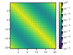
(a) $A^{-1}$

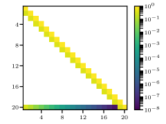
(b) $L$

Figure 3: Decay in the inverse and $L$-factor of the matrix from Example 3.12.

Example 3.12.

Consider the $n\times n$ matrix

$$A(i,j):=\begin{cases}3&\text{if }i=j\\ -1&\text{if }i=j\pm 1\mod n,\\ 0&\text{otherwise}\\ \end{cases}$$

whose graph structure for $n=6$ is illustrated in Fig. 1. We observe that $\mathrm{level}(n,j)=j-1$ increases monotonically from $j=1$ to $j=n-2$ and thus $L(n,j)$ decreases monotonically over the same range, see Fig. 3b. Conversely, $d(n,j)=\min\{j,n-j\}$ has a maximum at $j=\tfrac{n}{2}$ and thus $|A^{-1}(n,j)|$ has a minimum at this value of $j$, see Fig. 3a.

4 Incomplete selected inversion

Theorems 3.5 and 3.9 assert that $L(i,j)$ and $A^{-1}(i,j)$ are small if their indices $i$ and $j$ are far apart according to the appropriate notion of distance, which suggests that it should be possible to ignore such entries without losing much accuracy. Following this idea, we will next present incomplete factorization and selected inversion algorithms (Algorithms 4 and 5) which have been obtained by modifying Algorithms 1 and 3 such that they operate on only the entries $L(i,j)$ and $A^{-1}(i,j)$ with indices $(i,j)$ from the restricted set

(22) $$\mathrm{ifnz}(H):=\big{\{}(i,j)\in\mathrm{fnz}(H)\mid\mathrm{level}(i,j)\leq c\big{\}}$$

for some $c>0$. Of course, such a modification is only worth considering if it leads to a substantial improvement in performance and negligible loss of accuracy; hence the main topic of this section will be to assess these two performance metrics.

It is easily seen that restricting the selected inversion algorithm to $\mathrm{ifnz}(H)$ results in linear-scaling computational costs.

Theorem 4.1.

The runtime and memory requirements of Algorithms 4 and 5 (incomplete factorization and incomplete selected inversion) are given by

(23) $$\begin{cases}\mathcal{O}(nc)&\text{if }d=2,\\ \mathcal{O}(nc^{3})&\text{if }d=3,\end{cases}\qquad\text{and}\qquad\begin{cases}\mathcal{O}(n\log(c))&\text{if }d=2,\\ \mathcal{O}(nc)&\text{if }d=3,\end{cases}$$

respectively, where $d$ denotes the effective dimension of the problem in the sense of Table 1 and a nested dissection order is assumed.

Proof 4.2.

Nested dissection ordering of $G(A)$ splits the vertices into $\mathcal{O}\bigl{(}nc^{-d}\bigr{)}$ localized clusters $\mathcal{C}_{k}$ of diameter $\mathcal{O}(c)$ (the white squares in Fig. 2) separated by a complementary set $\mathcal{S}$ of

(24) $$\text{(number of $d-1$-dimensional slices)}\times\text{(number of vertices per slice)}=\ldots$$

(25) $$=\mathcal{O}\bigl{(}n^{1/d}\,c^{-1}\bigr{)}\times\mathcal{O}\bigl{(}n^{(d-1)/d}\bigr{)}=\mathcal{O}\bigl{(}nc^{-1}\bigr{)}$$

vertices (the colored bars in Fig. 2). On each of the clusters $\mathcal{C}_{k}$, incomplete selected inversion proceeds as in the exact algorithm and therefore requires

$$\begin{cases}\mathcal{O}\bigl{(}(c^{2})^{3/2}\bigr{)}=\mathcal{O}\bigl{(}c^{3}\bigr{)}&\text{if }d=2,\\ \mathcal{O}\bigl{(}(c^{3})^{2}\bigr{)}=\mathcal{O}\bigl{(}c^{6}\bigr{)}&\text{if }d=3\\ \end{cases}$$

runtime and

$$\begin{cases}\mathcal{O}\bigl{(}c^{2}\,\log(c^{2})\bigr{)}=\mathcal{O}\bigl{(}c^{2}\,\log(c)\bigr{)}&\text{if }d=2,\\ \mathcal{O}\bigl{(}(c^{3})^{4/3}\bigr{)}=\mathcal{O}\bigl{(}c^{4}\bigr{)}&\text{if }d=3\\ \end{cases}$$

memory. Multiplying these estimates by the number of clusters $\mathcal{O}\bigl{(}nc^{-d}\bigr{)}$ yields the estimates given in Eq. 23. Each vertex $v$ in the separator set $\mathcal{S}$ is fill-path-connected to $\mathcal{O}\bigl{(}c^{d-1}\bigr{)}$ vertices in $\mathcal{S}$ and to

$$\mathcal{O}\left(\sum_{k=0}^{\log_{2}(c)}2^{(d-1)\,k}\right)=\mathcal{O}\bigl{(}c^{d-1}\bigr{)}$$

vertices in the localized clusters $\mathcal{C}_{k}$ adjacent to $v$, where the second estimate follows from the fact that $v$ can be fill-path-connected to at most $V_{\mathrm{sep}}$ and some subset of either $V_{1}$ or $V_{2}$ but not both for each triplet $V_{1},V_{2},V_{\mathrm{sep}}$ encountered by the nested dissection algorithm (Algorithm 2) applied to the localized clusters $\mathcal{C}_{k}$ adjacent to $v$. It follows from closer inspection of Algorithms 4 and 5 (incomplete factorization and selected inversion) that the part of the selected inversion algorithm associated with $\mathcal{S}$ requires

(26) $$\#\mathcal{S}\times\mathrm{nfpn}^{2}=\mathcal{O}\bigl{(}nc^{-1}\bigr{)}\times\mathcal{O}\bigl{(}c^{2(d-1)}\bigr{)}=\mathcal{O}\bigl{(}nc^{2d-3}\bigr{)}$$

runtime and

(27) $$\#\mathcal{S}\times\mathrm{nfpn}=\mathcal{O}\bigl{(}nc^{-1}\bigr{)}\times\mathcal{O}\bigl{(}c^{d-1}\bigr{)}=\mathcal{O}\bigl{(}nc^{d-2}\bigr{)},$$

memory, where $\mathrm{nfpn}$ denotes the number of fill-path-neighbors per $v\in\mathcal{S}$. These estimates agree with those given in Eq. 23 up to the logarithmic factor for the memory requirements in the case $d=2$.

The following result summarizes our findings regarding the accuracy of incomplete selected inversion.

Theorem 4.3.

Assuming 4.13, Section 4.1 and 4.22, the entries $B(i,j)$ computed by Algorithms 4 and 5 (incomplete factorization and incomplete selected inversion) satisfy the bound

$$\big{\|}(H-zI)^{-1}-B\big{\|}_{\mathrm{nz}(H)}\lesssim_{\varepsilon}\exp\bigl{(}-2\,g_{\mathcal{E}}(z)\,c\bigr{)}$$

where $\|A\|_{\mathcal{I}}$ denotes the supremum norm on $\mathcal{I}\subset\{1,\ldots,n\}^{2}$,

$$\|A\|_{\mathcal{I}}:=\max_{(i,j)\in\mathcal{I}}|A(i,j)|.$$

Three particularities of Theorem 4.3 deserve further comment. Firstly, we note Theorem 4.3 predicts a convergence speed which is twice as fast as one might expect based on Theorems 3.5 and 3.9, namely $2g_{\mathcal{E}}(z)$ rather than $g_{\mathcal{E}}(z)$. This observation can be intuitively explained by noting that the entries $L(i,j)$ dropped by the incomplete algorithm have magnitudes $\lesssim_{\varepsilon}\exp\bigl{(}-g_{\mathcal{E}}(z)\,c\bigr{)}$ but occur at entries $i,j$ which are at least a distance $\mathrm{level}(i,j)>c$ away from the nonzeros of $H$. Propagating the resulting errors to $\mathrm{nz}(H)$ therefore attenuates them by an additional factor $\exp\bigl{(}-g_{\mathcal{E}}(z)\,c\bigr{)}$ which yields the final error estimate given in Theorem 4.3. Secondly, we observe that Theorem 4.3 is based on some conjectures which are plausible and confirmed by numerical evidence but which we have not been able to establish rigorously. This circumstance somewhat tarnishes our result from a theoretical point of view, but we expect it to have no practical consequences. Finally, we remark that the assumption referenced in Theorem 4.3 was only introduced to simplify the statement of the result and has little impact regarding the generality of our findings.

The remainder of this section is devoted to the proof of Theorem 4.3. Specifically, Section 4.1 will establish in Corollary 4.16 a result analogous to Theorem 4.3 for the incomplete factorization step, and Section 4.2 will do the same for the incomplete selected inversion step in Corollary 4.24. Theorem 4.3 will then follow from Corollaries 4.16 and 4.24 by a simple application of the triangle inequality.

Definition 4.4.

This section follows the notation of Definitions 2.2 and 3.4 with $A=H-zI$ as well as the following additions.

• $\tilde{r}:=\{k\in r\mid(k,j)\in\mathrm{ifnz}(H)\}$ with $j$ and $r$ as in Definition 2.2.

• $c$ denotes the cut-off level-of-fill from Eq. 22.

• $\tilde{L},\tilde{D}$ denote the incomplete $LDL^{T}$ factors and $E$ denotes the dropped entries computed in Algorithm 4. Furthermore, we set $\tilde{A}:=\tilde{L}\tilde{D}\tilde{L}^{T}$.

• $B(i,j)\approx A^{-1}(i,j)$ denotes the approximate entries of the inverse and $F$ denotes the dropped entries computed in Algorithm 5.

• In both Algorithms 4 and 5, we assume that matrix entries which are not specified are set to zero.

4.1 Incomplete $LDL^{T}$ Factorization

Restricting Algorithm 1 to $\mathrm{ifnz}(H)$ yields the following incomplete $LDL^{T}$ factorization (see Definition 4.4 for notation).

Algorithm 4 Incomplete $LDL^{T}$ factorization

1:for $j=1,\ldots,n$ do

2:     $\tilde{D}(j,j)=A(j,j)-\tilde{L}(j,\ell)\,\tilde{D}(\ell,\ell)\,\tilde{L}^{T}(\ell,j)$

3:     $\tilde{L}(\tilde{r},j)=\big{(}A(\tilde{r},j)-\tilde{L}(\tilde{r},\ell)\,\tilde{D}(\ell,\ell)\,\tilde{L}^{T}(\ell,j)\big{)}/\tilde{D}(j,j)$

4:     $E(r\setminus\tilde{r},j)=\tilde{L}(r\setminus\tilde{r},\ell)\,\tilde{D}(\ell,\ell)\,\tilde{L}^{T}(\ell,j)$

5:     $E(j,r\setminus\tilde{r})=E(r\setminus\tilde{r},j)^{T}$

6:end for

Algorithm 4 is precisely the symmetric version of the well-known incomplete LU factorization commonly used as a preconditioner in iterative methods for linear systems, see e.g. [Saa03, §10.3]. Keeping track of the dropped entries $E$ in 4 and 5 is not required in an actual implementation, but doing so in Algorithm 4 allows us to conveniently formulate the following results regarding the errors introduced by restricting the sparsity pattern of $L$.

Theorem 4.5 ([Saa03, Proposition 10.4]).

In the notation of Definition 4.4, we have that $\tilde{L}\tilde{D}\tilde{L}^{T}=A+E$.

Proof 4.6.

We note that $\mathrm{level}(i,j)>0$ for all $i\in r\setminus\tilde{r}$; hence $A(r\setminus\tilde{r},j)=0$ and

$$A(r\setminus\tilde{r},j)+E(r\setminus\tilde{r},j)-\tilde{L}(r\setminus\tilde{r},\ell)\,\tilde{D}(\ell,\ell)\,\tilde{L}^{T}(\ell,j)=0$$

according to 4 of Algorithm 4. Since $E(\tilde{r},j)=0$ and $\tilde{L}(r\setminus\tilde{r},j)=0$, we can thus combine 3 and 4 to

(28) $$\tilde{L}(r,j)=\big{(}A(r,j)+E(r,j)-\tilde{L}(r,\ell)\,\tilde{D}(\ell,\ell)\,\tilde{L}^{T}(r,j)\big{)}/\tilde{D}(j,j),$$

and similarly we can rewrite 2 as

(29) $$\tilde{D}(j,j)=A(j,j)+E(j,j)-\tilde{L}(j,\ell)\,\tilde{D}(\ell,\ell)\,\tilde{L}^{T}(\ell,j).$$

The claim follows after noting that Eqs. 28 and 29 are precisely the recursion formulae of the exact $LDL^{T}$ factorization in Algorithm 1 applied to the symmetric matrix $A+E$.

Theorem 4.7.

In the notation of Definition 4.4 and assuming $\|E\|_{2}<\delta:=\min|z-\mathcal{E}|$, we have that

(30) $$\big{|}\big{(}(H-zI)^{-1}-(H+E-zI)^{-1}\big{)}(i,j)\big{|}\lesssim_{\varepsilon}\ldots$$

$$\lesssim_{\varepsilon}\sum_{\tilde{\imath},\tilde{\jmath}=1}^{n}\exp\Bigl{(}-g_{\mathcal{E}}(z)\,\big{(}d(i,\tilde{\imath})+d(\tilde{\jmath},j)\big{)}\Bigr{)}\,\big{|}E(\tilde{\imath},\tilde{\jmath})\big{|}+\frac{\delta^{-2}\,\|E\|_{2}^{2}}{\delta-\|E\|_{2}}.$$

This bound is illustrated in Fig. 4a.

Proof 4.8.

Expanding $(H+E-zI)^{-1}$ in a Neumann series around $H-zI$, we obtain

(31) $$(H-zI)^{-1}-(H+E-zI)^{-1}=\ldots$$

$$=(H-zI)^{-1}\,E\,(H-zI)^{-1}-\sum_{k=2}^{\infty}\big{(}-(H-zI)^{-1}\,E\big{)}^{k}\,(H-zI)^{-1}.$$

The claim follows by estimating the entries of $(H-zI)^{-1}$ in the first term using Theorem 3.5 and bounding the entries of the second term through its operator norm.

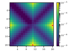
(a) $|A^{-1}-\tilde{A}^{-1}|$

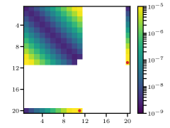
(b) $|\tilde{A}^{-1}-B|$

Figure 4: Error introduced by the incomplete selected factorization step (left) and incomplete selected inversion step (right) applied to the matrix from Example 3.12 with a cut-off level-of-fill $c=9$. The red dots mark the nonzero entries in $E$ and $F$, respectively.

Theorem 4.7 provides an a-posteriori error estimate for the inverse $(H+E-zI)^{-1}$ in terms of the dropped entries $E$, which could be used in an adaptive truncation scheme where $\mathrm{ifnz}(H)$ is of the form

(32) $$\mathrm{ifnz}(H)=\big{\{}(i,j)\in\mathrm{fnz}(H)\mid|\tilde{L}(i,j)|\geq\tau\big{\}}$$

for some tolerance $\tau\geq 0$, see [Saa03, §10.4]. Conversely to the level-of-fill-based scheme from Eq. 22, such a tolerance-based scheme would control the error but not the amount of fill-in since the perturbed entries $|\tilde{L}(i,j)|$ may fail to be small even when the corresponding entries $L(i,j)$ are small. Both schemes thus require further information about the perturbed factor $\tilde{L}$ or equivalently about the dropped entries $E(i,j)$ in order to simultaneously control the accuracy and the computational effort. Specifically, in the case of the level-of-fill scheme Eq. 22 we need to understand

• the sparsity pattern of $E$ since this impacts the number of terms and the size of the exponential factor in Eq. 30, and

• the magnitudes of the nonzero entries $E(\tilde{\imath},\tilde{\jmath})$.

The first of these two points is easily addressed.

Lemma 4.9.

In the notation of Definition 4.4, we have that

$$E(i,j)\neq 0\quad\implies\quad c<\mathrm{level}(i,j)\leq 2c+1.$$

In particular, the number of nonzero entries per row or column of $E$ is bounded independently of $n$.

The proof of this result will make use of the following lemma.

Lemma 4.10.

In the notation of Definition 4.4 and barring cancellation, we have that $E(i,j)\neq 0$ if and only if $(i,j)\in\mathrm{fnz}(H)\setminus\mathrm{ifnz}(H)$ and there exists a $k\in\ell$ such that $(i,k),(j,k)\in\mathrm{ifnz}(H)$.

Proof 4.11.

The claim follows by noting that 4 in Algorithm 4 performs a nonzero update on $E(i,j)$ if and only if

$$i\in r\setminus\tilde{r}\quad\iff\quad(i,j)\in\mathrm{fnz}(H)\setminus\mathrm{ifnz}(H)$$

and there exists a $k\in\ell$ such that

(33) $$\tilde{L}(i,k)\,\tilde{L}(j,k)\neq 0\quad\iff\quad(i,k),(j,k)\in\mathrm{ifnz}(H).$$

Proof 4.12 (Proof of Lemma 4.9).

According to Lemma 4.10, we have that

$$E(i,j)\neq 0\implies(i,j)\in\mathrm{fnz}(H)\setminus\mathrm{ifnz}(H)\implies\mathrm{level}(i,j)>c.$$

To derive the upper bound on $\mathrm{level}(i,j)$, let us assume that $E(i,j)\neq 0$. Then, Lemma 4.10 guarantees that there exists a vertex $k\in\ell$ such that $i,k$ and $j,k$ are connected by fill paths of lengths at most $c+1$ (recall from Definition 3.8 that the level-of-fill is the length of the shortest path minus 1). Concatenating these two paths yields a fill path between $i$ and $j$ of length at most $2c+2$; hence $\mathrm{level}(i,j)\leq 2c+1$. Finally, the claim regarding the sparsity of $E$ follows from the fact that there are at most $\mathcal{O}\bigl{(}c^{d}\bigr{)}$ vertices $i$ within a distance $2c+1$ from a fixed vertex $j$ in a graph associated with a problem of effective dimension $d$.

Regarding the second of the above points, namely the magnitudes of the dropped entries $E(\tilde{\imath},\tilde{\jmath})$, we expect that the following result holds.

Conjecture 4.13.

In the notation of Definition 4.4, we have that

$$|E(i,j)|\lesssim_{\varepsilon}\exp\bigl{(}-g_{\mathcal{E}}(z)\,\mathrm{level}(i,j)\bigr{)}.$$

Proof 4.14 (Discussion).

Reversing the substitutions in the proof of Theorem 2.3, we obtain

$$E(i,j)=\tilde{L}(i,\ell)\,\tilde{D}(\ell,\ell)\,\tilde{L}^{T}(\ell,j)=\tilde{A}(i,\ell)\,\tilde{A}(\ell,\ell)^{-1}\,\tilde{A}(\ell,j),$$

and expanding the latter formula to first order in $\|E\|_{2}$ as in Theorem 4.7 yields

(34) $$E(i,j) =A(i,\ell)\,A(\ell,\ell)^{-1}\,A(\ell,j)\ldots$$

$$\qquad+E(i,\ell)\,A(\ell,\ell)^{-1}\,A(\ell,j)\ldots$$

$$\qquad-A(i,\ell)\,A(\ell,\ell)^{-1}E(\ell,\ell)\,A(\ell,\ell)^{-1}\,A(\ell,j)\ldots$$

$$\qquad+A(i,\ell)\,A(\ell,\ell)^{-1}\,E(\ell,j)+\mathcal{O}\bigl{(}\|E\|^{2}_{2}\bigr{)}.$$

Theorem 3.9 guarantees that the first term

$$A(i,\ell)\,A(\ell,\ell)^{-1}\,A(\ell,j)=L(i,j)\,D(j,j)$$

on the right-hand side of Eq. 34 satisfies $\big{|}L(i,j)\,D(j,j)\big{|}\lesssim_{\varepsilon}\exp\bigl{(}-g_{\mathcal{E}}(z)\,c\bigr{)}$, but bounding the remaining terms is challenging because the magnitudes of these terms recursively depend on the errors committed earlier.

To illustrate this point, let us assume we have a bound $|E(\tilde{\imath},\tilde{\jmath})|\leq C_{0}$ with $C_{0}\sim\exp\bigl{(}-g_{\mathcal{E}}(z)\,c\bigr{)}$ for all entries of $E$ on the right-hand side of Eq. 34 such that we can bound e.g. the second term by

(35) $$\big{|}E(i,\ell)\,A(\ell,\ell)^{-1}\,A(\ell,j)\big{|}\leq C_{0}\,\sum_{k\in\ell}\big{|}A_{\ell}^{-1}(k,\ell)\,A(\ell,j)\big{|}$$

where $A_{\ell}:=A(\ell,\ell)$. From the sparsity of $A(\ell,j)$ and the localization of $A_{\ell}^{-1}$, it then follows that the sum on the right-hand side of Eq. 35 decays exponentially for an appropriate ordering of the terms and can therefore be bounded by some constant $C$ independent of $n$. In general, this constant $C$ will be larger than one, however, since some $k\in\ell$ may well be close to $j$ in terms of the graph distance on $G(A_{\ell})$ such that the corresponding terms are not small. Bounding the other terms in Eq. 34 similarly, we thus obtain $|E(i,j)|\leq C\,C_{0}$ for some constant $C>1$.

For the next entry $E(i^{\prime},j^{\prime})$ to be estimated using Eq. 34, the entry $E(i,j)$ that we just estimated may now appear on the right-hand side such that we have to assume the bound $|E(\tilde{\imath}^{\prime},\tilde{\jmath}^{\prime})|\leq C\,C_{0}$ for these entries. Proceeding analogously as above, we then obtain the bound $|E(i^{\prime},j^{\prime})|\leq C^{2}\,C_{0}$ which is worse by a factor of $C>1$ than the bound in the preceding step and worse by a factor of $C^{2}>1$ than the bound two steps ago. We therefore conclude that any estimate on the dropped entries $E(i,j)$ deteriorates exponentially with every recursive application of Eq. 34.

The key issue in the above analysis is that without further knowledge about the entries $E(i,j)$, we have to assume that all the error terms in the recursion formula Eq. 34 accumulate rather than cancel. We conjecture that such an accumulation of errors cannot occur, at least for matrices which are “well-behaved” in a suitable sense, but a rigorous proof of this claim requires deeper insight into the structure of the incomplete $LDL^{T}$ factorization and is left for future work.

4.13 suggests that the incomplete factorization exhibits the same localization as the exact factorization, which is in principle enough to derive an a-priori bound from the a-posteriori bound in Theorem 4.7. However, we introduce one more assumption in order to simplify the final result.

Either $\mathrm{level}(i,j)=\infty$ or $\mathrm{level}(i,j)\leq C\,d(i,j)$ for some $C>0$ independent of $i,j$ and $n$.

Proof 4.15 (Discussion).

We have seen in Example 3.12 that this assumption is not satisfied in the case of one-dimensional periodic chains, but we expect that this counterexample is the proverbial exception which proves the rule. In particular, we conjecture that Section 4.1 is always satisfied in dimensions $d>1$ and if a nested dissection order is used, since in this case every pair of vertices is connected by many paths and it seems unlikely that the nested dissection order would place a high-numbered vertex on all the short paths. This hypothesis is supported by our numerical experiments presented in Example 5.2 below. Furthermore, we will see in Example 5.3 that even if Section 4.1 is violated, the conclusions that we draw from it still hold up to some minor modifications.

Corollary 4.16.

In the notation of Definition 4.4, and assuming 4.13 and Section 4.1, we have that

$$\big{\|}(H-zI)^{-1}-(H+E-zI)^{-1}\big{\|}_{\mathrm{nz}(H)}\lesssim_{\varepsilon}\exp\bigl{(}-2\,g_{\mathcal{E}}(z)\,c\bigr{)}.$$

Proof 4.17.

It follows from Lemma 4.9 (sparsity of $E$) and 4.13 (localization of $E$) that for all $\tilde{\imath},\tilde{\jmath}\in\{1,\ldots,n\}$ we have that $|E(\tilde{\imath},\tilde{\jmath})|\lesssim_{\varepsilon}\exp\bigl{(}-g_{\mathcal{E}}(z)\,c\bigr{)}.$ Inserting this estimate into the bound from Theorem 4.7 (a-posteriori error bound) yields

(36) $$\big{|}\big{(}(H-zI)^{-1}-(H+E-zI)^{-1}\big{)}(i,j)\big{|}\lesssim_{\varepsilon}\ldots$$

$$\lesssim_{\varepsilon}\sum_{(\tilde{\imath},\tilde{\jmath})\in\mathrm{nz}(E)}\exp\Bigl{(}-g_{\mathcal{E}}(z)\,\big{(}d(i,\tilde{\imath})+d(\tilde{\jmath},j)+c\big{)}\Bigr{)}+\frac{\delta^{-2}\,\|E\|_{2}^{2}}{\delta-\|E\|_{2}}.$$

We are only interested in entries $(i,j)\in\mathrm{nz}(H)$ for which $d(i,j)\leq 1$; thus we conclude from the triangle inequality and Section 4.1 ($d(i,j)\gtrsim\mathrm{level}(i,j)$) that for all $(\tilde{\imath},\tilde{\jmath})\in\mathrm{nz}(E)$ we have that

$$d(i,\tilde{\imath})+d(\tilde{\jmath},j)+1\geq d(\tilde{\imath},\tilde{\jmath})\gtrsim\mathrm{level}(\tilde{\imath},\tilde{\jmath})\geq c+1.$$

In particular, we note that if $d(i,\tilde{\imath})\lesssim\frac{c}{2}$, then $d(\tilde{\jmath},j)\gtrsim\frac{c}{2}$ and vice versa, which allows us to bound the first term in Eq. 36 by

(37) $$\sum_{(\tilde{\imath},\tilde{\jmath})\in\mathrm{nz}(E)}\exp\Bigl{(}-g_{\mathcal{E}}(z)\,\big{(}d(i,\tilde{\imath})+d(\tilde{\jmath},j)+c\big{)}\Bigr{)}\lesssim\ldots$$

(38) $$\lesssim 2\sum_{\begin{subarray}{c}\tilde{\imath}\text{ such that}\\ d(i,\tilde{\imath})\lesssim\frac{c}{2}\end{subarray}}\,\,\sum_{\begin{subarray}{c}\tilde{\jmath}\text{ such that}\\ d(\tilde{\jmath},j)\gtrsim c-d(i,\tilde{\imath})\end{subarray}}\exp\Bigl{(}-g_{\mathcal{E}}(z)\,\big{(}d(i,\tilde{\imath})+d(\tilde{\jmath},j)+c\big{)}\Bigr{)}+\ldots$$

(39) $$\qquad\qquad+\sum_{\begin{subarray}{c}\tilde{\imath}\text{ such that}\\ d(i,\tilde{\imath})\gtrsim\frac{c}{2}\end{subarray}}\,\,\sum_{\begin{subarray}{c}\tilde{\jmath}\text{ such that}\\ d(\tilde{\jmath},j)\gtrsim\frac{c}{2}\end{subarray}}\exp\Bigl{(}-g_{\mathcal{E}}(z)\,\big{(}d(i,\tilde{\imath})+d(\tilde{\jmath},j)+c\big{)}\Bigr{)}$$

(40) $$\lesssim_{\varepsilon}\exp\bigl{(}-2\,g_{\mathcal{E}}(z)\,c\bigr{)}$$

where on the last line we estimated the infinite sums using the boundedness of the geometric series and the finite sum over $\tilde{\imath}$ was estimated as the largest term in the sum times the bounded number of terms.

The second term in Eq. 36 can be bounded using Gershgorin’s circle theorem and the facts that all diagonal entries satisfy $E(i,i)=0$, all off-diagonal entries satisfy $|E(i,j)|\lesssim_{\varepsilon}\exp\bigl{(}-g_{\mathcal{E}}(z)\,c\bigr{)}$, and the number of off-diagonal entries is bounded independently of $n$, which yields $\|E\|_{2}\lesssim_{\varepsilon}\exp\big{(}-g_{\mathcal{E}}(z)\,c\bigr{)}$. The claim then follows by combining the bounds on the two terms in Eq. 36.

4.2 Incomplete Selected Inversion

Restricting Algorithm 3 to $\mathrm{ifnz}(H)$ yields the following incomplete selected inversion algorithm (see Definition 4.4 for notation).

Algorithm 5 Incomplete selected inversion

1:for $j=n,\ldots,1$ do

2:     $B(\tilde{r},j)=-B(\tilde{r},\tilde{r})\,\tilde{L}(\tilde{r},j)$

3:     $B(j,\tilde{r})=B(\tilde{r},j)^{T}$

4:     $B(j,j)=\tilde{D}(j,j)^{-1}-B(j,\tilde{r})\,\tilde{L}(\tilde{r},j)$

5:     $F(r\setminus\tilde{r},j)=B(r\setminus\tilde{r},\tilde{r})\,\tilde{L}(\tilde{r},j)$

6:     $F(j,r\setminus\tilde{r})=F(r\setminus\tilde{r},j)^{T}$

7:     $F(j,j)=F(j,\tilde{r})\,\tilde{L}(\tilde{r},j)$

8:end for

As in Algorithm 4, keeping track of the dropped entries $F$ on 5, 6 and 7 is not required in an actual implementation but doing so facilitates our discussion of the errors committed by this algorithm.

Our error analysis for Algorithm 5 proceeds along the same lines as in Section 4.1: we first establish an a-posteriori bound in terms of the dropped entries $F$ in Theorem 4.20, then we argue that $|F(i,j)|$ should decay like $|A^{-1}(i,j)|$ in 4.22, and finally we derive an a-priori bound based on this conjecture in Corollary 4.24. For all of these steps, we will need the following result which establishes that $\tilde{A}^{-1}=(A+E)^{-1}$ exhibits the same localization as $A^{-1}$.

Lemma 4.18.

In the notation of Definition 4.4 and assuming 4.13, we have that

$$|\tilde{A}^{-1}(i,j)|\lesssim_{\varepsilon}\exp\bigl{(}-g_{\mathcal{E}}(z)\,d(i,j)\bigr{)}.$$

Proof 4.19.

According to Theorem 4.7 (a-posteriori error bound for $\tilde{A}^{-1}$), Lemma 4.9 (sparsity of $E$) and 4.13 (localization of $E$), we have that

(41) $$|\tilde{A}^{-1}(i,j)| \lesssim_{\varepsilon}|A^{-1}(i,j)|+\sum_{(\tilde{\imath},\tilde{\jmath})\in\mathrm{nz}(E)}\exp\Bigl{(}-g_{\mathcal{E}}(z)\,\big{(}d(i,\tilde{\imath})+c+d(\tilde{\jmath},j)\big{)}\Bigr{)}.$$

The claim follows by estimating the first term on the right hand side using Theorem 3.5 (localization of $A^{-1}$) and the second term using the boundedness of geometric series.

Theorem 4.20.

In the notation of Definition 4.4 and assuming 4.13, we have that

(42) $$\Big{|}\big{(}\tilde{A}^{-1}-B\big{)}(i,j)\Big{|} \lesssim_{\varepsilon}\sum_{\tilde{\jmath}\,=j+1}^{n}\exp\bigl{(}-g_{\mathcal{E}}(z)\,\mathrm{level}(\tilde{\jmath},j)\bigr{)}\,|F(i,\tilde{\jmath})|+\ldots$$

$$\qquad+\sum_{\tilde{\imath},\tilde{\jmath}\,=j+1}^{n}\exp\Bigl{(}-g_{\mathcal{E}}(z)\,\big{(}\mathrm{level}(i,\tilde{\imath})+\mathrm{level}(\tilde{\jmath},j)\big{)}\Bigr{)}\,|F(\tilde{\imath},\tilde{\jmath})|.$$

This bound is illustrated in Fig. 4b.

Proof 4.21.

Let us first consider the application of Algorithm 3 (exact selected inversion) to the matrix $\tilde{A}=A+E=\tilde{L}\tilde{D}\tilde{L}^{T}$. We note that the entries $\tilde{A}^{-1}(i^{\prime},j^{\prime})$ computed by this algorithm after iteration $j$ depend only on $\tilde{L}(\cdot,\ell)$, $\tilde{D}(\ell,\ell)$ and $\tilde{A}^{-1}(\bar{r},\bar{r})$, hence iterations $j^{\prime}=j-1,\ldots,1$ may be interpreted as a map $\phi:\big{(}\tilde{L}(\cdot,\ell),\tilde{D}(\ell,\ell),\tilde{A}^{-1}(\bar{r},\bar{r})\bigr{)}\mapsto\tilde{A}^{-1}$ which must be unique since the map from $\tilde{A}^{-1}$ to $\big{(}\tilde{L}(\cdot,\ell),\tilde{D}(\ell,\ell),\tilde{A}^{-1}(\bar{r},\bar{r})\bigr{)}$ is injective. This uniqueness allows us to determine $\phi$ by applying selected inversion to the block-$LDL^{T}$ factorization from Eq. 9, which yields

(43) $$\tilde{A}^{-1}=\left(\begin{smallmatrix}\tilde{A}(\ell,\ell)^{-1}+\tilde{A}(\ell,\ell)^{-1}\tilde{A}(\ell,\bar{r})\,\tilde{A}^{-1}(\bar{r},\bar{r})\,\tilde{A}(\bar{r},\ell)\,\tilde{A}(\ell,\ell)^{-1}\quad&-\tilde{A}(\ell,\ell)^{-1}\tilde{A}(\ell,\bar{r})\,\tilde{A}^{-1}(\bar{r},\bar{r})\\[5.0pt] \phantom{\tilde{A}(\ell,\ell)^{-1}\tilde{A}(\ell,\ell)^{-1}\tilde{A}(\ell,\bar{r})\,}-\tilde{A}^{-1}(\bar{r},\bar{r})\,\tilde{A}(\bar{r},\ell)\,\tilde{A}(\ell,\ell)^{-1}\quad&\phantom{-\tilde{A}(\ell,\ell)^{-1}\tilde{A}(\ell,\bar{r})\,}\tilde{A}^{-1}(\bar{r},\bar{r})\\ \end{smallmatrix}\right).$$

Note that this is indeed a map in terms of $\tilde{L}(\cdot,\ell)$, $\tilde{D}(\ell,\ell)$ since all of the submatrices in Eq. 43 other than $\tilde{A}(\bar{r},\bar{r})^{-1}$ can be computed from $\tilde{L}(\cdot,\ell)$, $\tilde{D}(\ell,\ell)$.

Let us now assume for the moment that Algorithm 5 (incomplete selected inversion) only drops entries in $B\bigl{(}\bar{r},j\bigr{)}$ and $B\bigl{(}j,\bar{r}\bigr{)}$ such that

$$B(\bar{r},\bar{r})=\tilde{A}^{-1}(\bar{r},\bar{r})+F(\bar{r},\bar{r}).$$

Since by assumption the incomplete inversion does not perform any additional mistakes after iteration $j$, we have that $B=\phi\bigl{(}B(\bar{r},\bar{r})\bigr{)}$ where for brevity we dropped the arguments of $\phi$ other than $\tilde{A}^{-1}(\bar{r},\bar{r})$, and since $\phi$ is affine in $\tilde{A}^{-1}(\bar{r},\bar{r})$ it further follows that

(44) $$\begin{array}[]{r @{{}={}} c @{{}+{}} l}B=\phi\bigl{(}B(\bar{r},\bar{r})\bigr{)}&\phi\bigl{(}\tilde{A}^{-1}(\bar{r},\bar{r})\bigr{)}&\phi\bigl{(}F(\bar{r},\bar{r})\bigr{)}-\phi(0)\\ &\tilde{A}^{-1}&\phi\bigl{(}F(\bar{r},\bar{r})\bigr{)}-\phi(0).\end{array}$$

In the simplified case where errors occur only in $B\bigl{(}\bar{r},j\bigr{)}$ and $B\bigl{(}j,\bar{r}\bigr{)}$, the claim then follows by estimating the entries of $\phi\bigl{(}F(\bar{r},\bar{r})\bigr{)}-\phi(0)$ using the localization of $\tilde{A}(\ell,\ell)^{-1}$ described in Lemma 4.18. The general estimate follows by applying Eq. 44 repeatedly for each $j$.

Conjecture 4.22.

In the notation of Definition 4.4, we have that

$$|F(i,j)|\lesssim_{\varepsilon}\exp\bigl{(}-g_{\mathcal{E}}(z)\,d(i,j)\bigr{)}.$$

Proof 4.23 (Discussion).

From the proof of Theorem 4.20, it follows that $F$ can be computed recursively according to

(45) $$F(i,j)=\tilde{A}^{-1}(i,j)-F\bigl{(}i,r(i)\bigr{)}\,M^{T}\bigl{(}r(i),j\bigr{)}+M\bigl{(}i,r(j)\bigr{)}\,F\bigl{(}r(j),r(j)\bigr{)}\,M^{T}\bigl{(}r(j),j\bigr{)}$$

where

$$M(i,\tilde{\imath})=\begin{cases}A_{\ell(\tilde{\imath})}^{-1}\bigl{(}i,\ell(\tilde{\imath})\bigr{)}\,A\bigr{(}\ell(\tilde{\imath}),\tilde{\imath}\bigr{)}&i<\tilde{\imath}\\ 0&\text{otherwise}\end{cases}$$

and $A_{\ell}:=A(\ell,\ell)$. Proving 4.22 thus faces the same obstacle as 4.13, namely that the errors committed at iteration $j$ depend on errors committed at previous iterations $j^{\prime}>j$ such that any bound deteriorates exponentially in the recursion depth.

Corollary 4.24.

In the notation of Definition 4.4, and assuming 4.13, Section 4.1 and 4.22, we have that

$$\big{\|}(H+E-zI)^{-1}-B^{-1}\big{\|}_{\mathrm{nz}(H)}\lesssim_{\varepsilon}\exp\bigl{(}-2\,g_{\mathcal{E}}(z)\,c\bigr{)}.$$

Proof 4.25.

Analogous to Corollary 4.16.

5 Numerical experiments

This section illustrates the theory presented in this paper at the example of a toy Hamiltonian $H\in\mathbb{R}^{n\times n}$ with entries $H(i,j)$ given by

(46) $$H(i,j):=\begin{cases}(-1)^{d(i,1)}&\text{if }i=j,\\ -\tfrac{1}{2d}&\text{if }i\sim j,\\ 0&\text{otherwise},\\ \end{cases}$$

where $d\in\{1,2,3\}$ denotes the dimension and $i\sim j$ if $i$ and $j$ are nearest neighbors in a $d$-dimensional Cartesian mesh with periodic boundary conditions. We note that the off-diagonal entries $H(i,j)=-\frac{1}{2d}$ correspond to a shifted and scaled finite-difference discretization of the $d$-dimensional Laplace operator, and the diagonal entries $H(i,i)=(-1)^{d(i,1)}$ take the form of a chequerboard pattern where each vertex has the opposite sign compared to its neighbors. In two and three dimensions, we use the nested dissection order illustrated in Fig. 2 to improve the sparsity of the $LDL^{T}$ factorization, while in one dimension we use a simple left-to-right order as shown in Fig. 1. All numerical experiments have been performed on a single core of an Intel Core i7-8550 CPU (1.8 GHz base frequency, 4 GHz turbo boost) using the Julia programming language [BEKS17]. A Julia package developed as part of this work is available at https://github.com/ettersi/IncompleteSelectedInversion.jl.

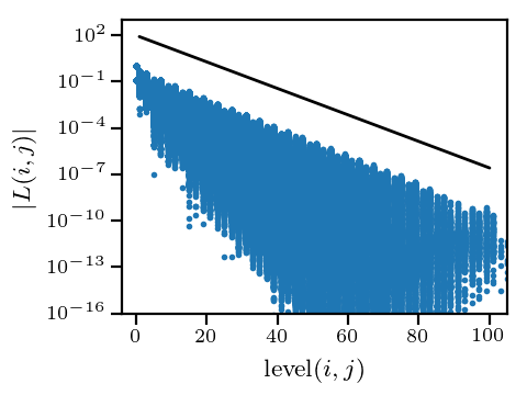
(a) Factorization

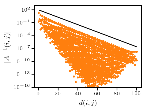
(b) Inverse

Figure 5: Localization of the $L$-factor (a) and inverse (b) of the matrix $H-0.98I$ with $H$ constructed according to Eq. 46 with $d=2$ and $\sqrt{n}=100$. The black lines indicate the rate of decay $g_{\mathcal{E}}(z)$ predicted by Theorems 3.5 and 3.9.

Example 5.1 (localization).

The chequerboard pattern along the diagonal causes the spectrum of $H$ to cluster in the two intervals $\mathcal{E}:=[-\sqrt{2},-1]\cup[1,\sqrt{2}]$ such that one may think of $H$ as the Hamiltonian matrix of an insulator with band gap $(-1,1)$. Figure 5 compares the entries of the $LDL^{T}$ factorization and inverse of $H-zI$ against the predictions of Theorems 3.5 and 3.9, and we observe that the theory is matched perfectly. In particular, the entries of the $L$-factor decay with the same rate $g_{\mathcal{E}}(z)$ as the inverse, which indicates that the spectra of all leading submatrices of $H$ are indeed contained in $\mathcal{E}$ as conjectured in Remark 3.11.

The excellent agreement between the theoretical and empirical convergence rates is a consequence of the simple sparsity pattern in Eq. 46, and the agreement may be worse for a more realistic Hamiltonian.

Example 5.2 (scaling and convergence).

Figure 6 numerically confirms the $\mathcal{O}(nc)$ ($d=2$) and $\mathcal{O}(nc^{3})$ ($d=3$) scaling of incomplete selected inversion predicted by Theorem 4.1. Furthermore, Fig. 7 demonstrates that incomplete selected inversion indeed converges exponentially in the cut-off level-of-fill $c$ with a rate of convergence equal to twice the localization rate $g_{\mathcal{E}}(z)$ as predicted in Theorem 4.3.

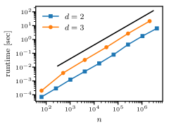
(a) Scaling in $n$ for $c=4$

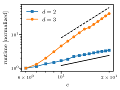
(b) Scaling in $c$ for $n^{1/d}=32$

Figure 6: Scaling of the incomplete selected inversion algorithm with respect to the matrix size $n$ (left) and cut-off level-of-fill $c$ (right). The black lines indicate $\mathcal{O}(n)$ scaling (Figure (a)), $\mathcal{O}(c)$ scaling (Figure (b), solid) and $\mathcal{O}(c^{3})$ scaling (Figure (b), dashed) as predicted by Theorem 4.1. The reported runtimes are the minimum out of three runs of selected inversion applied to the matrix $H$ from Eq. 46. In Figure (b), the runtimes have been scaled by $1/\text{runtime}(c=6)$ to ensure comparable y-values for the two plots.

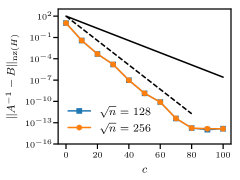
(a) $d=2,z=0.98$

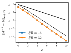
(b) $d=3,z=0$

Figure 7: Error vs. cut-off level-of-fill $c$ of incomplete factorization and selected inversion algorithm applied to $A=H-zI$ with $H$ as in Eq. 46. The solid black lines indicate exponential decay with rate $g_{\mathcal{E}}(z)$, and the dashed lines indicate twice this rate.

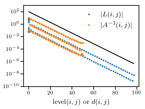
(a) Localization

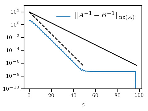
(b) Error

Figure 8: Localization (left) and convergence of incomplete factorization and selected inversion (right) of the matrix $H-zI$ with $H$ as in Eq. 46, $d=1$ $n=100$ and $z=0.98$. The solid black lines indicate exponential decay with rate $g_{\mathcal{E}}(z)$, and the dashed line indicates twice this rate.

Example 5.3.

Finally, we continue the discussion of Section 4.1 ($d(i,j)\gtrsim\mathrm{level}(i,j)$) which was used to derive Theorem 4.3 but which we have seen to be violated in the case of one-dimensional periodic chains. Figure 8 shows that even in this case, the incomplete algorithm converges with rate $2g_{\mathcal{E}}(z)$ as predicted by Theorem 4.3, but the convergence breaks down at a cut-off level-of-fill $c$ of about $\frac{n}{2}$ after which the error stagnates.

In the framework of Section 4, this observation may be explained as follows. Due to the simple graph structure of $H$, the matrix of dropped entries $E$ from Algorithm 4 contains precisely two nonzero entries at locations $i=n$, $j=c+2$ and the transpose thereof, and by 4.13 these entries satisfy

$$|E(n,c+2)|\lesssim_{\varepsilon}\exp\bigl{(}-g_{\mathcal{E}}(z)\,\mathrm{level}(n,c+2)\bigr{)}=\exp\bigl{(}-g_{\mathcal{E}}(z)\,(c+1)\bigr{)}.$$

(In this case, 4.13 can easily be proven since the incomplete factorization algorithm only drops a single entry.) According to Theorem 4.7, the error due to the incomplete factorization is thus upper-bounded by

(47) $$\|A^{-1}-\tilde{A}^{-1}\|_{\mathrm{nz}(A)} \lesssim_{\varepsilon}\max_{(i,j)\in\mathrm{nz}(A)}\exp\Bigl{(}-g_{\mathcal{E}}(z)\,\big{(}d(i,n)+c+1+d(c+2,j)\big{)}\Bigr{)}$$

(48) $$\lesssim_{\varepsilon}\exp\Bigl{(}-g_{\mathcal{E}}(z)\,\big{(}c+1+\min\{d(c+2,1),d(c+2,n-1)\}\big{)}\Bigr{)}$$

(49) $$=\begin{cases}\exp\bigl{(}-2\,g_{\mathcal{E}}(z)\,(c+1)\bigr{)}&\text{if }c\leq\tfrac{n-4}{2},\\ \exp\bigl{(}-g_{\mathcal{E}}(z)\,(n-2)\bigr{)}&\text{otherwise},\\ \end{cases}$$

and a similar bound can be derived for the error $\|\tilde{A}^{-1}-B\|_{\mathrm{nz}(A)}$ introduced by the incomplete selected inversion step. We note that Eq. 49 describes precisely the behaviour observed in Fig. 8b.

As discussed after Section 4.1, we expect that $d(i,j)\gtrsim\mathrm{level}(i,j)$ is rarely violated in dimensions $d>2$ and if a nested dissection vertex order is used. This example further demonstrates that even if Section 4.1 is violated, the incomplete selected inversion algorithm still converges at the rate $2g_{\mathcal{E}}(z)$ until the cut-off level-of-fill $c$ becomes $\mathcal{O}(n)$, at which point the speedup of the incomplete selected inversion compared to the exact algorithm vanishes anyway.

6 Conclusion

We have shown that the $LDL^{T}$ factorization of a sparse and well-conditioned matrix $A$ exhibits a localization property similar to that of $A^{-1}$, and we have developed algorithms which exploit this property to compute selected entries of $A^{-1}$ in $\mathcal{O}(n)$ runtime and memory. This opens up a new class of linear-scaling electronic structure algorithms which we expect to be highly competitive compared to existing algorithms due to reasons which we shall explain next.

Most linear-scaling electronic structure codes in use today proceed according to the following outline [Goe99, BM12].

• Express the density matrix $f_{\beta,E_{F}}(H)$ as the minimizer of some functional $\mathcal{F}:\mathbb{R}^{n\times n}\to\mathbb{R}$,

  $$f_{\beta,E_{F}}(H)=\operatorname*{arg\,min}_{\Gamma\in\mathbb{R}^{n\times n}}\mathcal{F}(\Gamma).$$

• Compute an approximation $\tilde{\Gamma}\approx f_{\beta,E_{F}}(H)$ with $\mathcal{O}(n)$ effort by minimizing $\mathcal{F}(\tilde{\Gamma})$ over the space of matrices with a certain prescribed sparsity pattern.

For simplicity of our argument, we will assume that the functional $\mathcal{F}(\Gamma)$ is given by the McWeeny purification function [McW60]

$$\mathcal{F}(\Gamma):=\operatorname{Tr}\Bigl{(}\big{(}3\Gamma^{2}-2\Gamma^{3}\big{)}\,(H-\mu I)\Bigr{)}$$

and the minimization is performed using the conjugate gradients algorithm, but we expect that similar observations also hold for more sophisticated linear-scaling schemes. The bulk of the compute time is then spent on evaluating products of sparse matrices, each of which requires $\mathcal{O}\bigl{(}nc^{2d}\bigr{)}$ floating-point operations assuming an effective dimension $d$ and that both matrix arguments have localization length $c$. Furthermore, the number of conjugate gradient steps and hence the number of matrix products required to reach a fixed accuracy scales with the inverse square root of the band gap in $H$ [Goe99, §III.D]. In contrast, the number of selected inversions required by the PEXSI scheme scales only logarithmically with the band gap and temperature [LLYE09, Mou16, Ett19], and each selected inversion with a localization length $c$ requires $\mathcal{O}\bigl{(}nc\bigr{)}$ operations for two-dimensional problems and $\mathcal{O}\bigl{(}nc^{3}\bigr{)}$ operations for three-dimensional problems; see Theorem 4.1. The incomplete PEXSI scheme thus makes order of magnitudes fewer calls to the low-level routine (selected inversion / matrix product) than the optimization scheme, and each such call runs faster for large enough $c$. Combining these two factors leads us to expect that our iPEXSI scheme will outperform existing linear-scaling algorithms at least in the regime of large enough localization lengths $c$.

As a case in point, we report that the selected inversion algorithm applied to the matrix Eq. 46 with $d=2$, $\sqrt{n}=256$ and $c=20$ takes 0.4 seconds, while evaluating the $20$th power of the same matrix $H$ takes 7.5 seconds (see Section 5 for details regarding hardware and software). Evaluating a power of $H$ with similar localization properties as those assumed in the selected inversion is roughly 20 times slower for these particular parameters, and this ratio will tip even further in favor of the selected inversion algorithm as we increase the localization length $c$.

What is needed next in order to realize the promised advantage of the iPEXSI algorithm is a massively parallel high-performance implementation of the incomplete selected inversion algorithm comparable to that presented for the exact algorithm in [JLY16]. Developing such a code will be the topic of future work, but we would like to point out that the parallelization strategies from [JLY16] also apply to the incomplete factorization and selected inversion algorithms and hence we expect similar parallel scaling. Closely related work regarding the parallel implementation of the incomplete LU factorization with arbitrary level-of-fills (as opposed to the more wide-spread ILU(0) and ILU(1) factorizations) can be found in [KK97, HP01, SZW03, DC11]. Furthermore, an alternative ILU algorithm based on iterative refinement of a trial factorization and designed specifically to improve parallel scaling has recently been proposed in [CP15]. While this algorithm was found to be highly effective at finding factorizations suitable for preconditioning, it is unclear whether it is applicable in the context of the selected inversion algorithm where the accuracy requirements are much more stringent. Additionally, the algorithm from [CP15] will only lead to an asymptotic speedup for the selected inversion algorithm if a similarly parallelizable algorithm for the selected inversion step can be developed. It is not obvious whether such an algorithm exists, since the algorithm from [CP15] is based on Theorem 4.5 which has no analogue for the selected inversion step.

References

- [BBR13] M. Benzi, P. Boito, and N. Razouk, Decay properties of spectral projectors with applications to electronic structure, SIAM Review, 55 (2013), pp. 3–64, doi:10.1137/100814019.
- [BEKS17] J. Bezanson, A. Edelman, S. Karpinski, and V. B. Shah, Julia: A fresh approach to numerical computing, SIAM Review, 59 (2017), pp. 65–98, doi:10.1137/141000671.
- [BM12] D. R. Bowler and T. Miyazaki, O(N) methods in electronic structure calculations, Reports on Progress in Physics, 75 (2012), doi:10.1088/0034-4885/75/3/036503.
- [CP15] E. Chow and A. Patel, Fine-grained parallel incomplete LU factorization, SIAM Journal on Scientific Computing, 37 (2015), pp. C169–C193, doi:10.1137/140968896.
- [Dav06] T. A. Davis, Direct Methods for Sparse Linear Systems, Society for Industrial and Applied Mathematics, 2006, doi:10.1137/1.9780898718881.
- [DC11] X. Dong and G. Cooperman, A bit-compatible parallelization for ILU(k) preconditioning, in European Conference on Parallel Processing, 2011, pp. 66–77, doi:10.1007/978-3-642-23397-5_8.
- [DMS84] S. Demko, W. F. Moss, and P. W. Smith, Decay rates for inverses of band matrices, Mathematics of Computation, 43 (1984), pp. 491–499, doi:10.1090/S0025-5718-1984-0758197-9.
- [ET75] A. M. Erisman and W. F. Tinney, On computing certain elements of the inverse of a sparse matrix, Communications of the ACM, 18 (1975), pp. 177–179, doi:10.1145/360680.360704.
- [Ett19] S. Etter, Polynomial and Rational Approximation for Electronic Structure Calculations, PhD thesis, University of Warwick, 2019, https://ettersi.github.io/pdf/phd.pdf.
- [Geo73] A. George, Nested dissection of a regular finite element mesh, SIAM Journal on Numerical Analysis, 10 (1973), pp. 345–363, doi:10.1137/0710032.
- [Gil88] J. R. Gilbert, Some nested dissection order is nearly optimal, Information Processing Letters, 26 (1988), pp. 325–328, doi:10.1016/0020-0190(88)90191-3.
- [Goe99] S. Goedecker, Linear scaling electronic structure methods, Reviews of Modern Physics, 71 (1999), pp. 1085–1123, doi:10.1103/RevModPhys.71.1085.
- [GV96] G. H. Golub and C. F. Van Loan, Matrix Computations, Johns Hopkins University Press, Baltimore, third ed., 1996.
- [HP01] D. Hysom and A. Pothen, A scalable parallel algorithm for incomplete factor preconditioning, SIAM Journal on Scientific Computing, 22 (2001), pp. 2194–2215, doi:10.1137/S1064827500376193.
- [JLY16] M. Jacquelin, L. Lin, and C. Yang, PSelInv – A distributed memory parallel algorithm for selected inversion, ACM Transactions on Mathematical Software, 43 (2016), doi:10.1145/2786977.
- [Kax03] E. Kaxiras, Atomic and Electronic Structure of Solids, Cambridge University Press, 2003, doi:10.1017/CBO9780511755545.
- [KK97] G. Karypis and V. Kumar, Parallel threshold-based ILU factorization, in Proceedings of the 1997 ACM/IEEE conference on Supercomputing, 1997, doi:10.1145/509593.509621.
- [Koh96] W. Kohn, Density functional and density matrix method scaling linearly with the number of atoms, Physical Review Letters, 76 (1996), pp. 3168–3171, doi:10.1103/PhysRevLett.76.3168.
- [LCYH13] L. Lin, M. Chen, C. Yang, and L. He, Accelerating atomic orbital-based electronic structure calculation via pole expansion and selected inversion, Journal of Physics: Condensed Matter, 25 (2013), doi:10.1088/0953-8984/25/29/295501.
- [LLY+09] L. Lin, J. Lu, L. Ying, R. Car, and W. E, Fast algorithm for extracting the diagonal of the inverse matrix with application to the electronic structure analysis of metallic systems, Communications in Mathematical Sciences, 7 (2009), pp. 755–777, doi:10.4310/CMS.2009.v7.n3.a12.
- [LLYE09] L. Lin, J. Lu, L. Ying, and W. E, Pole-based approximation of the Fermi-Dirac function, Chinese Annals of Mathematics, Series B, 30 (2009), pp. 729–742, doi:10.1007/s11401-009-0201-7.
- [McW60] R. McWeeny, Some recent advances in density matrix theory, Reviews of Modern Physics, 32 (1960), pp. 335–369, doi:10.1103/RevModPhys.32.335.
- [Mou16] J. E. Moussa, Minimax rational approximation of the Fermi-Dirac distribution, The Journal of Chemical Physics, 145 (2016), doi:10.1063/1.4965886.
- [OTC19] C. Ortner, J. Thomas, and H. Chen, Locality of interatomic forces in tight binding models for insulators, tech. report, 2019, arXiv:1906.11740.
- [Ran95] T. Ransford, Potential Theory in the Complex Plane, Cambridge University Press, 1995.
- [RT78] D. J. Rose and R. E. Tarjan, Algorithmic aspects of vertex elimination on directed graphs, SIAM Journal on Applied Mathematics, 34 (1978), pp. 176–197, doi:10.1137/0134014.
- [Saa03] Y. Saad, Iterative Methods for Sparse Linear Systems, Society for Industrial and Applied Mathematics, second ed., 2003, doi:10.1137/1.9780898718003.
- [Saf10] E. B. Saff, Logarithmic potential theory with applications to approximation theory, Surveys in Approximation Theory, 5 (2010), pp. 165–200, https://www.emis.de/journals/SAT/papers/14/.
- [SCS10] Y. Saad, J. R. Chelikowsky, and S. M. Shontz, Numerical methods for electronic structure calculations of materials, SIAM Review, 52 (2010), pp. 3–54, doi:10.1137/060651653.
- [SSW01] J. Shen, G. Strang, and A. J. Wathen, The potential theory of several intervals and its applications, Applied Mathematics and Optimization, 44 (2001), pp. 67–85, doi:10.1007/s00245-001-0011-0.
- [SZW03] C. Shen, J. Zhan, and K. Wang, Parallel multilevel block ILU preconditioning techniques for large sparse linear systems, in Proceedings International Parallel and Distributed Processing Symposium, 2003, doi:10.1109/IPDPS.2003.1213182.
- [TFC73] K. Takahashi, J. Fagan, and M.-S. Chin, Formation of a sparse bus impedence matrix and its application to short circuit study, in 8th PICA Conference Proceedings, 1973.
- [Tre13] L. N. Trefethen, Approximation Theory and Approximation Practice, Society for Industrial and Applied Mathematics, 2013.
- [Yan81] M. Yannakakis, Computing the minimum fill-in is NP-complete, SIAM Journal on Algebraic Discrete Methods, 2 (1981), pp. 77–79, doi:10.1137/0602010.