A proximal MM method for the zero-norm regularized PLQ composite optimization problem

Abstract

This paper is concerned with a class of zero-norm regularized piecewise linear-quadratic (PLQ) composite minimization problems, which covers the zero-norm regularized $\ell_{1}$-loss minimization problem as a special case. For this class of nonconvex nonsmooth problems, we show that its equivalent MPEC reformulation is partially calm on the set of global optima and make use of this property to derive a family of equivalent DC surrogates. Then, we propose a proximal majorization-minimization (MM) method, a convex relaxation approach not in the DC algorithm framework, for solving one of the DC surrogates which is a semiconvex PLQ minimization problem involving three nonsmooth terms. For this method, we establish its global convergence and linear rate of convergence, and under suitable conditions show that the limit of the generated sequence is not only a local optimum but also a good critical point in a statistical sense. Numerical experiments are conducted with synthetic and real data for the proximal MM method with the subproblems solved by a dual semismooth Newton method to confirm our theoretical findings, and numerical comparisons with a convergent indefinite-proximal ADMM for the partially smoothed DC surrogate verify its superiority in the quality of solutions and computing time.

Keywords: Zero-norm regularized PLQ composite problems; DC equivalent surrogates; nonconvex and nonsmooth; proximal MM method; semismooth Newton method

1 Introduction

Let $f\!:\mathbb{R}^{n}\!\to\mathbb{R}_{+}$ be a piecewise linear-quadratic nonsmooth convex function, $A\!\in\mathbb{R}^{n\times p}$ and $b\in\!\mathbb{R}^{n}$ be the given matrix and vector, and $\Omega\subseteq\!\mathbb{R}^{p}$ be a nonempty polyhedral set. We are interested in the following zero-norm regularized composite minimization problem

$$\min_{x\in\Omega}\Big{\{}f(Ax-b)+\frac{\mu}{2}\|x\|^{2}+\nu\|x\|_{0}\Big{\}}$$ (1)

where $\nu>0$ is a regularization parameter, $\|\cdot\|_{0}$ denotes the zero-norm (cardinality) of vectors, and $\mu>0$ is a small regularization parameter. The term $\frac{1}{2}\mu\|x\|^{2}$ is introduced to ensure that the objective function of (1) is coercive and then has a nonempty global optimum set. For convenience, we denote the sum of the first two functions by

$$F_{\mu}(x):=f(Ax-b)+(\mu/2)\|x\|^{2}\quad\ \forall x\in\mathbb{R}^{p}.$$ (2)

Since the zero-norm is the root to produce sparse solutions, the problem (1) has been found to have wide applications in a host of scientific and engineering problems such as regression and variable selection in statistics (see, e.g., [40, 16]), compressed sensing [14] and source separation [6] in signal processing, imaging decomposition [36] in image science, feature selection and classification in statistical learning [5, 46], and so on. In particular, the nonsmooth PLQ loss $f(Ax-b)$ makes the problem (1) arise frequently from robust models; for example, when $f(z)=\frac{1}{n}\sum_{i=1}^{n}\theta(z_{i})$ with $\theta(t)=|t|$ for $t\in\mathbb{R}$, it becomes the popular sparsity regularized $\ell_{1}$-loss minimization in robust sparse recovery [47, 26] and high-dimensional robust statistics [44, 42]; and when $\theta(t)=(\tau-\mathbb{I}_{\{t\leq 0\}})t$ for some $\tau\in(0,1)$, it reduces to the sparsity regularized check-loss minimization that is often used to monitor the heteroscedasticity of high-dimensional data [48, 43].

Owing to the combinatorial property of the zero-norm function, the problem (1) is generally NP-hard and it is impractical to seek a global minimum with an algorithm of polynomial-time complexity. For this class of nonconvex nonsmooth problems, a common way is to use the convex relaxation technique to achieve a desirable solution in a statistical sense. The $\ell_{1}$-norm convex relaxation, as a popular relaxation method, has witnessed considerable progress in theory and computation since the early works [13, 40]. Though the $\ell_{1}$-norm is the convex envelope of the zero-norm in the $\ell_{\infty}$-norm unit ball, its ability to promote sparsity is weak especially in a complicated constraint set, say, the simplex set. Inspired by this, many nonconvex surrogates have been proposed for the zero-norm function, which include the non-Lipschitz $\ell_{p}\ (0<p<1)$ surrogate [9, 10], smooth concave approximation [5, 32, 46], and the folded concave functions such as SCAD [16] and MCP [51]. All of these nonconvex surrogates are proposed from the primal viewpoint and the surrogate problems associated to the first two classes are only an approximation of (1). Although Soubies et al. [37] proposed a class of exact continuous relaxation for the $\ell_{2}$-$\ell_{0}$ minimization, their proof depends on the structure of the least-square loss function and it is not clear whether they are exact or not for the problem (1).

One contribution of this work is to show that an equivalent MPEC of (1) is partially calm on the set of global optima, thereby obtaining a family of equivalent DC surrogates from a primal-dual viewpoint. The calmness of a mathematical programming problem at a solution point was originally introduced by Clarke [11], and received active study from many researchers in the past several decades (see, e.g., [7, 49, 50]). Among others, Ye and Zhu [49, 50] extended it to the partial calmness at a solution point. Inspired by these works, Liu et al. [27] recently studied the partial calmness on the global optimum set for the equivalent MPECs of zero-norm and rank optimization problems so as to achieve their global exact penalty. By [27, Theorem 3.2], if a special structure is imposed on the set $\Omega$, such an MPEC is indeed partially calm on the set of global optima, but this structure is very restricted. Here we achieve this crucial property without any restriction on $\Omega$ by constructing an appropriate multifunction and using the upper Lipschitz continuity of the polyhedral multifunction due to Robinson [34]. Also, by combining this result with [27, Appendix B], we conclude that the SCAD is a member of this family of equivalent DC surrogates. Although Le Thi et al. [20] ever derived an equivalent DC surrogate for the zero-norm regularized problem from a primal-dual viewpoint, they required $\Omega$ to be a compact box set, and their surrogate has a great difference from ours; see Section 3.

Then, inspired by the work [39], we propose a proximal majorization-minimization (MM) method for solving one of the equivalent DC surrogate models, a semiconvex PLQ minimization problem involving three nonsmooth terms, by using a tighter majorization of the DC surrogate function. The other contribution of this work is to establish the global convergence and linear rate of convergence for the proximal MM method, and to demonstrate when the limit of the generated sequence is locally optimal to the surrogate problem and the origin problem (1), respectively. In particular, for the scenario where $f(z)=\frac{1}{n}\sum_{i=1}^{n}\theta(z_{i})$ with an appropriate convex $\theta\!:\mathbb{R}\to\mathbb{R}_{+}$ and the data $(b,A)$ comes from a linear observation model, we also derive an error bound to the true vector for the limit of the generated sequence, which shows that the limit is good from a statistical perspective. Numerical experiments are conducted with some synthetic and real data for the proposed proximal MM with the subproblems solved by a dual semismooth Newton method (PMMSN for short) to confirm our theoretical findings. In particular, we compare the performance of PMMSN with the performance of a globally convergent indefinite-proximal ADMM (iPADMM) proposed for solving the partially smoothed DC surrogate problem. Numerical comparisons indicate that PMMSN has an advantage in the quality of solutions and computing time for most of test examples, whereas iPADMM depends on the choice of the smoothing parameter that is very sensitive to the data.

It is worthwhile to emphasize that for optimization models involving a smooth loss term and a nonconvex surrogate of the zero-norm, there are some works to investigate the error bounds of their stationary points to the true vector (see, e.g., [25, 8]) or the oracle property of a local optimum yielded by a specific algorithm [17], but to the best of our knowledge, for optimization models involving a nonsmooth convex loss and such an equivalent DC surrogate, there are few works on the statistical error bound of the critical point yielded by an algorithm. The optimization model in [39] involves a square-root loss and such a DC surrogate, but the local optimality and statistical error bound of the obtained critical point was not discussed. For the box constrained zero-norm regularized nonsmooth convex loss minimization, Bian and Chen [4] recently presented an exact continuous relaxation and proposed a smoothing proximal gradient algorithm for finding a lifted stationary point of the relaxation model, but they did not provide a statistical error bound for the lifted stationary point. Also, as will be shown in Section 3, their continuous relaxation model is actually a member of our equivalent DC surrogates.

Notation: In this paper, $I$ and $e$ denote an identity matrix and a vector of all ones, respectively, whose dimensions are known from the context. For any matrix $X=[X_{ij}]_{n\times p}$, $\|X\|,\|X\|_{\infty}$ and $\!\interleave X\interleave_{1}$ denote the spectral norm, elementwise maximum norm and column sum norm of $A$, respectively, i.e., $\!\interleave X\interleave_{1}\!=\max_{1\leq j\leq p}\sum_{i=1}^{n}|X_{ij}|$, and for given index sets $\mathcal{I}\subseteq\{1,\ldots,n\}$ and $\mathcal{J}\subseteq\{1,\ldots,p\}$, $X_{\mathcal{I}\cdot}$ and $X_{\cdot\mathcal{J}}$ denote the matrix consisting of those rows $X_{i\cdot}$ of $X$ with $i\in\mathcal{I}$ and those columns $X_{\cdot j}$ of $X$ with $j\in\mathcal{J}$, respectively. For a set $S$, ${\rm conv}(S)$ means the convex hull of $S$ and $\delta_{S}$ denotes the indicator function of $S$, i.e., $\delta_{S}(x)=0$ if $x\in S$ and $+\infty$ otherwise. For given vectors $a,b\in\mathbb{R}^{p}$ with $a_{i}\leq b_{i}$ for each $i=1,\ldots,p$, the notation $[a,b]$ denotes the box set. For a vector $x$, $x_{\rm nz}$ represents the smallest nonzero entry of $x$ and $|x|^{\downarrow}$ denotes the vector obtained by arranging the entries of $|x|$ in a nonincreasing order. For an extended real-valued $f\!:\mathbb{R}^{p}\to[-\infty,+\infty]$, we say that $f$ is proper if $f(x)>-\infty$ for all $x\in\mathbb{R}^{p}$ and ${\rm dom}\,f\!:=\{x\in\mathbb{R}^{p}\ |\ f(x)<\infty\}\neq\emptyset$, and denote by $f^{*}$ the conjugate of $f$, i.e., $f^{*}(x^{*})\!:=\sup_{x\in\mathbb{R}^{p}}\{\langle x^{*},x\rangle-f(x)\}$. For a lower semicontinuous (lsc) function $f\!:\mathbb{R}^{p}\to(-\infty,+\infty]$ and a parameter $\gamma>0$, $\mathcal{P}_{\gamma}f$ and $e_{\gamma}f$ denote the proximal mapping and Moreau envelope of $f$, respectively, defined as

$$\mathcal{P}_{\gamma}f(x):=\mathop{\arg\min}_{z\in\mathbb{R}^{p}}\Big{\{}f(z)+\frac{1}{2\gamma}\|z-x\|^{2}\Big{\}}\ {\rm and}\ e_{\gamma}f(x):=\min_{z\in\mathbb{R}^{p}}\Big{\{}f(z)+\frac{1}{2\gamma}\|z-x\|^{2}\Big{\}}.$$

When $f$ is convex, $\mathcal{P}_{\gamma}f\!:\mathbb{R}^{p}\to\mathbb{R}^{p}$ is a Lipschitzian mapping with Lipschitz constant $1$, and $e_{\gamma}f$ is a smooth convex function with $\nabla e_{\gamma}f(x)=\gamma^{-1}(x-\mathcal{P}_{\gamma}f(x))$.

2 Preliminaries

First, we recall the concepts of the proximal, regular and limiting subdifferentials from [35, Definition 8.45 & 8.3] and the definition of the subderivative and second subderivative from [35, Definition 8.1 & 13.3] for an extended real-valued function.

2.1 Generalized subdifferentials and subderivatives

Definition 2.1

Consider a function $f\!:\mathbb{R}^{p}\to[-\infty,+\infty]$ and a point $x$ with $f(x)$ finite. The proximal subdifferential of $f$ at $x$, denoted by $\widetilde{\partial}\!f(x)$, is defined as

$$\widetilde{\partial}\!f(x):=\bigg{\{}v\in\mathbb{R}^{p}\ \big{|}\ \liminf_{x\neq x^{\prime}\to x}\frac{f(x^{\prime})-f(x)-\langle v,x^{\prime}-x\rangle}{\|x^{\prime}-x\|^{2}}>-\infty\bigg{\}};$$

the regular subdifferential of $f$ at $x$, denoted by $\widehat{\partial}\!f(x)$, is defined as

$$\widehat{\partial}\!f(x):=\bigg{\{}v\in\mathbb{R}^{p}\ \big{|}\ \liminf_{x\neq x^{\prime}\to x}\frac{f(x^{\prime})-f(x)-\langle v,x^{\prime}-x\rangle}{\|x^{\prime}-x\|}\geq 0\bigg{\}};$$

and the (limiting) subdifferential of $f$ at $x$, denoted by $\partial\!f(x)$, is defined as

$$\partial\!f(x):=\Big{\{}v\in\mathbb{R}^{p}\ |\ \exists\,x^{k}\to x\ {\rm with}\ f(x^{k})\to f(x)\ {\rm and}\ v^{k}\in\widehat{\partial}\!f(x^{k})\ {\rm with}\ v^{k}\to v\Big{\}}.$$

Remark 2.1

(i) At each $x\in{\rm dom}f$, the sets $\widetilde{\partial}f(x)$ and $\widehat{\partial}\!f(x)$ are always closed convex, $\partial\!f(x)$ is closed but generally nonconvex, and they satisfy $\widetilde{\partial}f(x)\subseteq\widehat{\partial}\!f(x)\subseteq\partial\!f(x)$. These inclusions may be strict when $f$ is nonconvex, and when $f$ is convex, they all reduce to the subdifferential of $f$ at $x$ in the sense of convex analysis [33].

(ii) The point $\overline{x}$ at which $0\in\partial\!f(\overline{x})$ (respectively, $0\in\widetilde{\partial}\!f(\overline{x})$ and $0\in\widehat{\partial}\!f(\overline{x})$) is called a limiting (respectively, proximal and regular) critical point of $f$. By [35, Theorem 10.1], a local minimizer of $f$ is necessarily a regular critical point of $f$, and then a limiting critical point. However, the converse may not hold; for example, the function $f(t)=-|t|+t$ for $t\in\mathbb{R}$ satisfies $0\in\partial\!f(0)$, but $0$ is not a local minimizer of $\min_{t\in\mathbb{R}}f(t)$.

(iii) Recall that a function $f\!:\mathbb{R}^{p}\to[-\infty,+\infty]$ is said to be semiconvex if there exists a constant $\gamma>0$ such that $x\mapsto f(x)+\frac{\gamma}{2}\|x\|^{2}$ is convex, and the smallest of all such $\gamma$ is called the semi-convex modulus of $f$. For this $f$, $\widetilde{\partial}\!f(x)=\widehat{\partial}\!f(x)=\partial\!f(x)$ at all $x\in{\rm dom}f$.

Definition 2.2

For a function $f\!:\mathbb{R}^{p}\to[-\infty,+\infty]$, a point $\overline{x}$ with $f(\overline{x})$ finite and any $v\in\mathbb{R}^{p}$, the subderivative function $df(\overline{x})\!:\mathbb{R}^{p}\to[-\infty,+\infty]$ is defined by

$$df(\overline{x})(w):=\liminf_{\tau\downarrow 0,\,w^{\prime}\to w}\frac{f(\overline{x}+\tau w^{\prime})-f(\overline{x})}{\tau},$$

while the second subderivative of $f$ at $\overline{x}$ for $v$ and $w$ is defined by

$$d^{2}f(\overline{x}|v)(w):=\liminf_{\tau\downarrow 0,\,w^{\prime}\to w}\frac{f(\overline{x}+\tau w^{\prime})-f(\overline{x})-\tau\langle v,w^{\prime}\rangle}{\frac{1}{2}\tau^{2}}.$$

2.2 Semismoothness of locally Lipschitzian mappings

Semismoothness was originally introduced by Mifflin [29] for functionals, and Qi and Sun [30] later developed the class of vector semismooth functions. Before introducing the semismoothness, we recall the Clarke Jacobian of a locally Lipschitzian mapping.

Definition 2.3

(see [12, Definition 2.6.1]) Let $F\!:\mathcal{O}\subseteq\mathbb{R}^{n}\to\mathbb{R}^{m}$ be a locally Lipschitzian mapping defined on an open set $\mathcal{O}$. Denote by $D_{F}\subseteq\mathcal{O}$ the set of points where $F$ is Fréchet differentiable and by $F^{\prime}(z)\in\mathbb{R}^{m\times n}$ the Jacobian of $F$ at $z\in D_{F}$. For any given $\overline{z}\in\mathcal{O}$, the Clarke (generalized) Jacobian of $F$ at $\overline{z}$ is defined as

$$\partial_{C}F(\overline{z}):={\rm conv}\Big{\{}\lim_{k\to\infty}F^{\prime}(z^{k})\ |\ \{z^{k}\}\subseteq D_{F}\ {\rm with}\ \lim_{k\to\infty}z^{k}=\overline{z}\Big{\}}.$$

Definition 2.4

(see [30, 38]) Let $F\!:\mathcal{O}\subseteq\mathbb{R}^{n}\to\mathbb{R}^{m}$ be a locally Lipschitzian mapping on an open set $\mathcal{O}$. The mapping $F$ is said to be semismooth at a point $x\in\mathcal{O}$ if $F$ is directionally differentiable at $x$ and for any $\Delta x\to 0$ and $V\in\partial_{C}F(x+\Delta x)$,

$$F(x+\Delta x)-F(x)-V\Delta x=o(\|\Delta x\|);$$

and $F$ is said to be strongly semismooth at $x$ if $F$ is semismooth at $x$ and for any $\Delta x\to 0$,

$$F(x+\Delta x)-F(x)-V\Delta x=O(\|\Delta x\|^{2}).$$

The mapping $F$ is said to be a semismooth (respectively, strongly semismooth) function on $\mathcal{O}$ if it is semismooth (respectively, strongly semismooth) everywhere in $\mathcal{O}$.

Lemma 2.1

Given $\omega\in\mathbb{R}_{+}^{p}$ and $\mu\geq 0$, let $h(x):=\|\omega\circ x\|_{1}+\frac{1}{2}\mu\|x\|^{2}$ for $x\in\mathbb{R}^{p}$. Then, $\mathcal{P}_{\gamma^{-1}}h(z)\!=\frac{\gamma}{\gamma+\mu}{\rm sign}(z)\circ\max(|z|-\omega/\gamma,0)$ for $z\in\mathbb{R}^{p}$ and its Clarke Jacobian is given by

$$\partial_{C}(\mathcal{P}_{\gamma^{-1}}h)(z)=\!\Big{\{}{\rm Diag}(v_{1},\ldots,v_{n})\ |\ v_{i}=\frac{\gamma}{\gamma\!+\!\mu}\ {\rm if}\ |z_{i}|>\frac{\omega_{i}}{\gamma},\,{\rm otherwise}\,v_{i}\in\big{[}0,\frac{\gamma}{\gamma\!+\!\mu}\big{]}\Big{\}}.$$

Notice that $\mathcal{P}_{\gamma^{-1}}h$ in Lemma 2.1 is piecewise affine. By [15, Proposition 7.4.7] every piecewise affine mapping is strongly semismooth. Hence, it is strongly semismooth.

3 Equivalent DC surrogates of problem (1)

Let $\mathscr{L}$ be the family of proper lsc functions $\phi\!:\mathbb{R}\to(-\infty,+\infty]$ with ${\rm int}({\rm dom}\,\phi)\supseteq[0,1]$ which are convex in the interval $[0,1]$ and satisfy the following conditions

$$1>t^{*}:=\mathop{\arg\min}_{0\leq t\leq 1}\phi(t),\ \phi(t^{*})=0\ \ {\rm and}\ \ \phi(1)=1.$$ (3)

Since $\phi(1)=1$ and $t^{*}$ is the unique minimizer of $\phi$ over $[0,1]$, for any $z\in\mathbb{R}^{p}$ we have

$$\|z\|_{0}=\min_{w\in\mathbb{R}^{p}}\Big{\{}{\textstyle\sum_{i=1}^{p}}\phi(w_{i})\quad\mbox{s.t.}\ \ \big{\langle}e-w,|z|\big{\rangle}=0,\,0\leq w\leq e\Big{\}}.$$

As far as we know, such a characterization for $z\in\mathbb{R}_{+}^{p}$ with $\phi(t)=t$ first appeared in [28]. This implies that the zero-norm regularized problem (1) is equivalent to the problem

$$\min_{x,w\in\mathbb{R}^{p}}\Big{\{}F_{\mu}(x)+\nu\textstyle{\sum_{i=1}^{p}}\phi(w_{i})\quad\mbox{s.t.}\ \ \langle e-w,|x|\rangle=0,\,x\in\Omega,\,w\in[0,e]\Big{\}}$$ (4)

in the following sense: if $x^{*}$ is globally optimal to the problem (1), then $(x^{*}\!,{\rm sign}(|x^{*}|))$ is a global optimal solution of the problem (4), and conversely, if $(x^{*},w^{*})$ is a global optimal solution of (4), then $x^{*}$ is globally optimal to (1). The problem (4) is a mathematical program with an equilibrium constraint $e-w\geq 0,|x|\geq 0,\langle e-w,|x|\rangle=0$. Although the MPEC is known to be very tough, in this section we can establish that the MPEC (4) is partially calm over its global optimal solution set, denoted by $\mathcal{S}^{*}$, and employ its relation with exact penalization to derive a class of equivalent DC surrogates for (1).

As mentioned in Section 1, when $\Omega$ has a special structure, the MPEC (4) is partially calm over the set $\mathcal{S}^{*}$ by [27, Theorem 3.2], but the required structure is very restricted. Here, we remove such a restriction and obtain the partial calmness of (4) over $\mathcal{S}^{*}$.

Proposition 3.1

The problem (4) is partially calm over the optimal solution set $\mathcal{S}^{*}$.

Proof: For each $\epsilon\in\!\mathbb{R}$, define the partial perturbation for the feasible set of (4) by

$$\mathcal{S}_{\epsilon}:=\big{\{}(x,w)\in\Omega\times[0,e]\ |\ \langle e-w,|x|\rangle=\epsilon\big{\}}.$$

Fix an arbitrary $(x^{*},w^{*})\in\mathcal{S}^{*}$. Notice that the objective function of the problem (4) is continuous. By [50, Remark 2.3], its partial calmness at $(x^{*},w^{*})$ is equivalent to the existence of $\delta>0$ and $\rho>0$ such that for all $\epsilon\in\mathbb{R}_{+}$ and all $(x,w)\in\mathbb{B}((x^{*},w^{*}),\delta)\cap\mathcal{S}_{\epsilon}$,

$$\big{[}F_{\mu}(x)+\nu{\textstyle\sum_{i=1}^{p}}\phi(w_{i})\big{]}-\big{[}F_{\mu}(x^{*})+\nu{\textstyle\sum_{i=1}^{p}}\phi(w_{i}^{*})\big{]}+\rho\nu\langle e-w,|x|\rangle\geq 0.$$ (5)

Observe that the solution set $\mathcal{S}^{*}$ is compact. There necessarily exists $R>0$ such that $\bigcup_{x^{*}\in\mathcal{S}^{*}}\mathbb{B}(x^{*},1/2)\subseteq\mathbb{B}_{R}:=\{x\in\mathbb{R}^{p}\ |\ \|x\|_{\infty}\leq R\}$. It is easy to check that the function $F_{\mu}$ is Lipschitzian relative to $\mathbb{B}_{R}$. We denote by $L_{F_{\mu}}$ the Lipschitz constant of $F_{\mu}$ over the set $\mathbb{B}_{R}$. For each $k\in\{1,2,\ldots,p\}$, define the multifunction $\Gamma^{k}\!:\mathbb{R}\rightrightarrows\mathbb{R}^{p}$ by

$$\Gamma^{k}(\tau):=\Big{\{}x\in\Omega\cap\mathbb{B}_{R}\ |\ \|x\|_{1}-\|x\|_{(k)}=\tau\Big{\}}$$

where $\|\cdot\|_{(k)}$ denotes the Ky Fan $k$-norm of vectors. Since $\Gamma^{k}$ is a polyhedral multifunction, i.e., its graph is the union of finitely many polyhedral convex sets, from [34, Proposition 1] it follows that each $\Gamma^{k}$ is calm at the origin for all $z\in\Gamma^{k}(0)$, which is equivalent to saying that for each $k\in\{1,\ldots,p\}$, there exist $\delta_{k}>0$ and $\gamma_{k}>0$ such that

$${\rm dist}(z,\Gamma^{k}(0))\leq\gamma_{k}\big{[}\|z\|_{1}-\|z\|_{(k)}\big{]}\quad\ \forall z\in\mathbb{B}(x^{*},\delta_{k}).$$ (6)

Set $\delta=\!\min\{\delta_{1},\ldots,\delta_{k},1/2\}$ and $\gamma=\!\max\{\gamma_{1},\ldots,\gamma_{k}\}$. Fix an arbitrary $\epsilon\geq 0$ and an arbitrary $(x,w)\in\mathbb{B}((x^{*},w^{*}),\delta)\cap\mathcal{S}_{\epsilon}$. Take an arbitrary $\rho\geq\frac{\gamma\phi_{-}^{\prime}(1)(1-t^{*})L_{F_{\mu}}}{\nu(1-t_{0})}$, where $t_{0}\in[0,1)$ is such that $\frac{1}{1-t^{*}}\in\partial\phi(t_{0})$ and its existence is shown in [27, Lemma 1]. Write

$$J:=\Big{\{}j\in\{1,2,\ldots,p\}\ |\ \rho|x|_{j}^{\downarrow}>\phi_{-}^{\prime}(1)\Big{\}}\ \ {\rm and}\ \ r=|J|.$$

Clearly, $x\in\mathbb{B}(x^{*},\delta_{r})$. By invoking (6) with $z=x$, there exists $\overline{x}^{\rho}\in\Gamma^{r}(0)$ such that

$$\|x-\overline{x}^{\rho}\|\leq\gamma\big{[}\|x\|_{1}-\|x\|_{(r)}\big{]}=\gamma{\textstyle\sum_{j=r+1}^{p}}|x|_{j}^{\downarrow}.$$ (7)

Let $J_{1}:=\big{\{}j\ |\ \frac{1}{1-t^{*}}\leq\rho|x|_{j}^{\downarrow}\leq\phi_{-}^{\prime}(1)\big{\}}$ and $J_{2}:=\big{\{}j\ |\ 0\leq\rho|x|_{j}^{\downarrow}<\frac{1}{1-t^{*}}\big{\}}$. Notice that

$$\sum_{i=1}^{p}\phi(w_{i}^{\downarrow})+\rho\big{(}\|x\|_{1}\!-\langle w,|x|\rangle\big{)}\geq\sum_{i=1}^{p}\min_{t\in[0,1]}\big{\{}\phi(t)+\rho|x|_{i}^{\downarrow}(1-t)\big{\}}.$$

By invoking [27, Lemma 1] with $\omega=|x|_{j}^{\downarrow}$ for each $j$, it immediately follows that

$${\textstyle\sum_{i=1}^{p}}\phi(w_{i}^{\downarrow})+\rho\big{(}\|x\|_{1}\!-\langle w,x\rangle\big{)}$$

$$\geq\|\overline{x}^{\rho}\|_{0}+\frac{\rho(1-t_{0})}{\phi_{-}^{\prime}(1)(1\!-t^{*})}\sum_{j\in J_{1}}\,|x|_{j}^{\downarrow}+\rho(1-t_{0})\sum_{j\in J_{2}}\,|x|_{j}^{\downarrow}$$

$$\geq\|\overline{x}^{\rho}\|_{0}+\frac{\rho(1-t_{0})}{\phi_{-}^{\prime}(1)(1\!-t^{*})}\sum_{j\in J_{1}\cup J_{2}}|x|_{j}^{\downarrow}=\|\overline{x}^{\rho}\|_{0}+\frac{\rho(1-t_{0})}{\phi_{-}^{\prime}(1)(1\!-t^{*})}\sum_{j=r+1}^{p}|x|_{j}^{\downarrow}$$

$$\geq\|\overline{x}^{\rho}\|_{0}+\frac{\rho(1-t_{0})}{\gamma\phi_{-}^{\prime}(1)(1\!-t^{*})}\|x-\overline{x}^{\rho}\|\geq\|\overline{x}^{\rho}\|_{0}+\nu L_{F_{\mu}}\|x-\overline{x}^{\rho}\|$$

where the second inequality is since $\phi(t^{*})-\phi(1)\geq\phi_{-}^{\prime}(1)(t^{*}\!-1)$, the third one is due to the inequality (7), the last is using $\rho\geq\frac{\gamma\phi_{-}^{\prime}(1)(1-t^{*})L_{F_{\mu}}}{\nu(1-t_{0})}$, and the equality is due to $J_{1}\cup J_{2}=\{1,\ldots,p\}\backslash J$ and $|J|=r$. Notice that $x\in\mathbb{B}_{R}$ since $\bigcup_{x^{*}\in\mathcal{S}^{*}}\mathbb{B}(x^{*},1/2)\subseteq\mathbb{B}_{R}$ and $\overline{x}^{\rho}\in\mathbb{B}_{R}$ by $\overline{x}^{\rho}\in\Gamma^{r}(0)$. From the Lipschitz continuity of $F_{\mu}$ over $\mathbb{B}_{R}$, it immediately follows that $L_{F_{\mu}}\|x-\overline{x}^{\rho}\|\geq F_{\mu}(\overline{x}^{\rho})-F_{\mu}(x).$ Combining with the last inequality, we obtain

$${\textstyle\sum_{i=1}^{p}}\phi(w_{i}^{\downarrow})+\rho\big{(}\|x\|_{1}\!-\langle w,x\rangle\big{)}\geq\|\overline{x}^{\rho}\|_{0}+\nu^{-1}\big{[}F_{\mu}(\overline{x}^{\rho})-F_{\mu}(x)\big{]}.$$ (8)

Now take $\overline{w}_{i}^{\rho}=1$ for $i\in{\rm supp}(\overline{x}^{\rho})$ and $\overline{w}_{i}^{\rho}=0$ for $i\notin{\rm supp}(\overline{x}^{\rho})$. Clearly, $(\overline{x}^{\rho},\overline{w}^{\rho})$ is a feasible point of the MPEC (4) with $\sum_{i=1}^{p}\phi(\overline{w}_{i}^{\rho})=\|\overline{x}^{\rho}\|_{0}$. Then, it holds that

$$F_{\mu}(\overline{x}^{\rho})+\nu\|\overline{x}^{\rho}\|_{0}\geq F_{\mu}(x^{*})+\nu{\textstyle\sum_{i=1}^{p}}\phi(w_{i}^{*}).$$

Together with the inequality (8), the stated inequality (5) holds. By the arbitrariness of $(x^{*},w^{*})$ in $\mathcal{S}^{*}$, we obtain the desired result. The proof is then completed. $\Box$

Notice that Proposition 3.1 still holds when $f$ is replaced by a general Lipschitzian function. Since the objective function of (4) is coercive relative to $\Omega\times[0,e]$, combining Proposition 3.1 with [27, Proposition 2.1(b)], we have the following conclusion.

Theorem 3.1

There exists a threshold $\overline{\rho}>0$ such that the following penalty problem

$$\min_{x\in\Omega,w\in[0,e]}\Big{\{}F_{\mu}(x)+\nu\big{[}\textstyle{\sum_{i=1}^{p}}\phi(w_{i})+\rho\langle e\!-\!w,|x|\rangle\big{]}\Big{\}}$$ (9)

associated to each $\rho\geq\overline{\rho}$ has the same global optimal solution set as the MPEC (4) does. Also, this conclusion holds when $f$ is replaced by a lower bounded Lipschitzian function.

Remark 3.1

By the proof of Proposition 3.1, it follows that $\overline{\rho}=\frac{\gamma\phi_{-}^{\prime}(1)(1-t^{*})L_{F_{\mu}}}{\nu(1-t_{0})}$, which depends on the Lipschitz constant of $F_{\mu}$ over the set $\mathbb{B}_{R}$, determined by $\mathcal{S}^{*}$, and the calmness constant $\gamma_{k}$ of $\Gamma^{k}$. So, it is generally hard to achieve an exact estimation on $\overline{\rho}$, and a varying $\rho$ is suggested in practical computation. We see that, as the regularization parameter $\nu$ increases, the corresponding threshold $\overline{\rho}$ becomes smaller, and consequently, it is easier to choose an appropriate $\rho$ such that (9) is a global exact penalty.

It is well known that the handling of nonconvex constraints is much harder than the handling of nonconvex objective functions. Thus, Theorem 3.1 provides a convenient way to deal with the difficult MPEC (4) and then the zero-norm regularized problem (1). In particular, the nonconvexity of the objective function of (9) is owing to the coupled term $\langle e-w,|x|\rangle$ rather than the combination. Such a structure ensures that the problem (9) associated to every $\rho>\overline{\rho}$ is an equivalent DC surrogate of (1). Indeed, by letting

$$\psi(t):=\!\left\{\!\begin{array}[]{cl}\phi(t)&\textrm{if}\ t\in[0,1];\\ +\infty&\textrm{otherwise}\end{array}\right.$$

and using the conjugate $\psi^{*}$ of $\psi$, the problem (9) can be compactly written as follows:

$$\min_{x\in\mathbb{R}^{p}}\Big{\{}\Theta_{\lambda,\rho}(x)\!:=F_{\mu}(x)+\delta_{\Omega}(x)+\lambda\|x\|_{1}-\lambda\rho^{-1}\textstyle{\sum_{i=1}^{p}}\psi^{*}(\rho|x_{i}|)\Big{\}}\ \ {\rm for}\ \lambda=\rho\nu.$$ (10)

Since $\psi^{*}$ is a nondecreasing finite convex function in $\mathbb{R}$, clearly, $\Theta_{\lambda,\rho}$ is a DC function and the problem (10) associated to every $\rho\geq\overline{\rho}$ is an equivalent DC surrogate of (1).

When $\phi(t)=t$ for $t\in\mathbb{R}$, clearly, $\phi\in\mathscr{L}$ with $t^{*}=0$. An elementary calculation yields that $\psi^{*}(s)=\max(s-1,0)$ for $s\in\mathbb{R}$. Now the last two terms $\|x\|_{1}-\rho^{-1}\sum_{i=1}^{p}\psi^{*}(\rho|x_{i}|)$ in $\Theta_{\lambda,\rho}(x)$ is precisely the continuous relaxation $\Phi(x)$ of the zero-norm given by [4]. For other choice of $\phi$, please refer to [27, Appendix B]. In the rest of this work, we focus on

$$\phi(t):=\frac{a-1}{a+1}t^{2}+\frac{2}{a+1}t~{}~{}(a>1)~{}~{}{\rm for}~{}~{}t\in\mathbb{R},$$ (11)

for which an elementary calculation yields that the conjugate $\psi^{*}$ has the following form

$$\psi^{*}(s)=\left\{\begin{array}[]{cl}0&\textrm{if}\ s\leq\frac{2}{a+1},\\ \frac{((a+1)s-2)^{2}}{4(a^{2}-1)}&\textrm{if}\ \frac{2}{a+1}<s\leq\frac{2a}{a+1},\\ s-1&\textrm{if}\ s>\frac{2a}{a+1}.\end{array}\right.$$ (12)

To close this section, we summarize the desirable properties of $\Theta_{\lambda,\rho}$ associated to this $\phi$. Their proofs are included in Appendix A where the following functions are needed:

$$g_{\rho}(x)\!:=\rho^{-1}{\textstyle\sum_{i=1}^{p}}\varphi_{\rho}(x_{i})\ \ {\rm with}\ \ \varphi_{\rho}(t):=\psi^{*}(\rho|t|)\ \ {\rm for}\ t\in\mathbb{R},$$ (13a)

$$w_{\rho}(x)\!:=((\psi^{*})^{\prime}(\rho|x_{1}|),\ldots,(\psi^{*})^{\prime}(\rho|x_{p}|))^{\mathbb{T}}\quad\ \forall x\in\mathbb{R}^{p}.\quad$$ (13b)

Proposition 3.2

For any given $\nu>0$ and $\rho>0$, the following results hold with $\lambda=\rho\nu$.

• $\Theta_{\lambda,\rho}$ is a lower bounded, coercive, semiconvex piecewise linear-quadratic function.

• For any given $x\in\mathbb{R}^{p}$, the generalized subdifferentials of $\Theta_{\lambda,\rho}$ at $x$ take the form of

  $$\!\widetilde{\partial}\Theta_{\lambda,\rho}(x)=\widehat{\partial}\Theta_{\lambda,\rho}(x)=\partial\Theta_{\lambda,\rho}(x)=A^{\mathbb{T}}\partial\!f(Ax\!-b)+\mu x+\mathcal{N}_{\Omega}(x)+\lambda\partial\|x\|_{1}-\lambda\nabla g_{\rho}(x).$$

• If $\overline{x}\in\mathbb{R}^{p}$ is a (limiting) critical point of $\Theta_{\lambda,\rho}$ with $|\overline{x}_{\rm nz}|\geq\frac{2a}{\rho(a+1)}$, then $\overline{x}$ is also a regular critical point of the zero-norm regularized problem (1).

• The function $\Theta_{\lambda,\rho}$ is a KL function of exponent $1/2$.

4 Proximal MM method for the problem (10)

By Proposition 3.2 (i) and the discussion in the last section, the zero-norm regularized composite problem (1) is equivalent to a piecewise linear-quadratic minimization problem (10) associated to $\rho>\overline{\rho}$. Although the objective function of (10) consists of a smooth $g_{\rho}$ with Lipschitzian gradient and a proper convex function $F_{\mu}(\cdot)+\|\cdot\|_{1}+\delta_{\Omega}(\cdot)$, this composite convex function makes the common proximal gradient method inapplicable to it. By introducing an additional variable $z\!\in\mathbb{R}^{n}$, the problem (10) can be rewritten as

$$\min_{x\in\mathbb{R}^{p},z\in\mathbb{R}^{n}}\Big{\{}f(z)+\frac{1}{2}\mu\|x\|^{2}+\lambda\|x\|_{1}-\lambda g_{\rho}(x)\ \ {\rm s.t.}\ \ Ax-z=b,\ x\in\Omega\Big{\}}$$ (14)

so that the ADMM can be applied to solving it, but to the best of our knowledge there is no convergence guarantee for the ADMM to such a nonconvex nonsmooth problem. It is worthwhile to point out that the results developed in [45] for the ADMM is not suitable for the problem (14). Motivated by the specific structure of $\Theta_{\lambda,\rho}$ and the recent work by Tang et al. [39], we in this section develop a tailored proximal MM method for (10).

Fix an arbitrary $x^{\prime}\in\mathbb{R}^{p}$. For any $x\in\mathbb{R}^{p}$, the convexity and smoothness of $\psi^{*}$ implies

$${\textstyle\sum_{i=1}^{p}}\psi^{*}(\rho|x_{i}|)\geq{\textstyle\sum_{i=1}^{p}}\psi^{*}(\rho|x_{i}^{\prime}|)+\langle w_{\rho}(x^{\prime}),\rho|x|-\rho|x^{\prime}|\rangle$$ (15)

where $w_{\rho}\!:\mathbb{R}^{p}\to\mathbb{R}^{p}$ is the mapping defined in (13b). Along with the expression of $\Theta_{\lambda,\rho}$,

$$\Theta_{\lambda,\rho}(x)\leq\Xi_{\lambda,\rho}(x,x^{\prime})\!:=\!F_{\mu}(x)+\delta_{\Omega}(x)+\lambda\|x\|_{1}-\lambda\langle w_{\rho}(x^{\prime}),|x|\rangle+R_{\lambda,\rho}(x^{\prime})$$

where $R_{\lambda,\rho}(x^{\prime})=\lambda\langle w_{\rho}(x^{\prime}),|x^{\prime}|\rangle-\lambda\rho^{-1}\!\sum_{i=1}^{p}\psi^{*}\big{(}\rho|x_{i}^{\prime}|\big{)}$. Notice that $\Xi_{\lambda,\rho}(x^{\prime},x^{\prime})=\Theta_{\lambda,\rho}(x^{\prime})$. This means that $\Xi_{\lambda,\rho}(\cdot,x^{\prime})$ is a majorization of $\Theta_{\lambda,\rho}$ at $x^{\prime}$. This majorization is tighter than the one in [39] obtained by the convexity of $g_{\rho}$. Indeed, by Lemma 1 in Appendix,

$$\langle w_{\rho}(x^{\prime}),|x|-|x^{\prime}|\rangle=\langle w_{\rho}(x^{\prime}),|x|\rangle-\langle\nabla g_{\rho}(x^{\prime}),x^{\prime}\rangle\geq\langle\nabla g_{\rho}(x^{\prime}),x\rangle-\langle\nabla g_{\rho}(x^{\prime}),x^{\prime}\rangle$$

where the inequality is using $[w_{\rho}(x^{\prime})]_{i}\geq 0$ for each $i$, and consequently for any $x\in\mathbb{R}^{p}$,

$$\Xi_{\lambda,\rho}(x,x^{\prime})\leq F_{\mu}(x)+\delta_{\Omega}(x)+\lambda\|x\|_{1}-\lambda\langle\nabla g_{\rho}(x^{\prime}),x\rangle+R_{\lambda,\rho}(x^{\prime}).$$

The majorization on the right hand side is precisely the one used by Tang et al. [39].

Our proximal MM method is designed by minimizing a proximal version of the majorization $\Xi(\cdot,x^{k})$ at the $k$th step, and its iterate steps are described as follows.

Algorithm 1 (Proximal MM method for solving (10))

Initialization: Choose a small $\mu>0$. Select $\lambda>0,\gamma_{1,0}>0,\gamma_{2,0}>0$, $\underline{\gamma_{1}}>0,\underline{\gamma_{2}}>0$ and $\varrho\in(0,1]$. Seek a starting point $x^{0}\in\Omega$ and a suitable $\rho\geq 1$. Set $k:=0$.

while the stopping conditions are not satisfied do

1. Let $w^{k}=w_{\rho}(x^{k})$. Compute the optimal solution $x^{k+1}$ of the following problem

   $$\min_{x\in\Omega}\Big{\{}F_{\mu}(x)+\lambda\langle e-w^{k},|x|\rangle+\frac{\gamma_{1,k}}{2}\|x-x^{k}\|^{2}+\frac{\gamma_{2,k}}{2}\|Ax-Ax^{k}\|^{2}\Big{\}}.$$ (16)

2. Update the proximal parameters $\gamma_{1,k}$ and $\gamma_{2,k}$ by the following rule

   $$\gamma_{1,k+1}=\max(\underline{\gamma_{1}},\varrho\gamma_{1,k})\ \ {\rm and}\ \ \gamma_{2,k+1}=\max(\underline{\gamma_{2}},\varrho\gamma_{1,k}).$$

3. Let $k\leftarrow k+1$, and go to Step 1.

end while

Remark 4.1

(i) Although the problem (10) is a DC program, Algorithm 1 does not belong to the DCA framework in [21] since $w^{k}\neq\nabla g_{\rho}(x^{k})$ by Lemma 1 in Appendix A. In fact, by the definition of $w_{\rho}$ in (13b) and the expression of $\psi^{*}$, it is easy to obtain that

$$w_{i}^{k}=\min\Big{[}1,\max\Big{(}0,\frac{(a\!+\!1)\rho|x_{i}^{k}|-2}{2(a\!-\!1)}\Big{)}\Big{]}\ \ {\rm for}\ i=1,\ldots,p.$$ (17)

The proximal term $\frac{\gamma_{1,k}}{2}\|x-x^{k}\|^{2}+\frac{\gamma_{2,k}}{2}\|Ax-Ax^{k}\|^{2}$ involved in the subproblems, inspired by the recent work [39], plays a twofold role: one is to ensure that the subproblem (16) is solvable and the other, as will be shown in the sequel, is to guarantee the decreasing of the objective value sequence of the nonconvex problem (10) and then its global convergence.

(ii) It is well known that for nonconvex optimization problems, the choice of the starting point determines the quality of the limit of the sequence generated from this initial point. This means that the choice of $x^{0}$ in Algorithm 1 is very crucial. Inspired by the good performance of $\ell_{1}$-norm regularized problem, we recommend to use the following $x^{0}$:

$$x^{0}\approx\!\mathop{\arg\min}_{x\in\mathbb{R}^{p}}\Big{\{}f(Ax\!-b)+\lambda\|x\|_{1}+\frac{\gamma_{1,0}}{2}\|x\|^{2}+\frac{\gamma_{2,0}}{2}\|Ax-b\|^{2}+\delta_{\Omega}(x)\Big{\}}.$$ (18)

As will be shown in Subsection 4.3, such an $x^{0}$ is not bad at least in a statistical sense. In addition, we suggest that the parameter $\rho$ is chosen by $\frac{c}{\|x^{0}\|_{\infty}}$ for a suitable $c>0$. By combining formula (17) with the term $\langle e-w^{k},|x|\rangle$ in (16), such a choice of $\rho$ ensures that those very small $x_{i}^{0}$ (very likely corresponding to a zero entry) becomes zero quickly since a weight close to $1$ is imposed on $|x_{i}|$, those very large $x_{i}^{0}$ (very likely corresponding to a nonzero entry) continue to be large since a weight closed to $0$ is imposed on $|x_{i}|$, and for the rest, a smaller $c$ means a larger weight imposed on them.

(iii) By the definition of $x^{k}$ and [33, Theorem 23.8], it follows that for each $k\in\mathbb{N}$,

$$0 \in\partial F_{\mu}(x^{k})+\mathcal{N}_{\Omega}(x^{k})+\lambda\big{[}(1-w_{1}^{k-1})\partial|x_{1}^{k}|\times\cdots\times(1-w_{p}^{k-1})\partial|x_{p}^{k}|\big{]}$$

$$\quad+\gamma_{1,k-1}(x^{k}-x^{k-1})+\gamma_{2,k-1}A^{\mathbb{T}}A(x^{k}-x^{k-1});$$ (19)

while by Proposition 3.2(ii) and Lemma 1 in Appendix A, it holds that

$$\partial\Theta_{\lambda,\rho}(x^{k}) =\partial F_{\mu}(x^{k})+\mathcal{N}_{\Omega}(x^{k})+\lambda\big{[}\partial|x_{1}^{k}|\times\cdots\times\partial|x_{p}^{k}|\big{]}-\lambda w^{k}\circ{\rm sign}(x^{k})$$

$$=\partial F_{\mu}(x^{k})+\mathcal{N}_{\Omega}(x^{k})+\lambda\big{[}(1-w_{1}^{k})\partial|x_{1}^{k}|\times\cdots\times(1-w_{p}^{k})\partial|x_{p}^{k}|\big{]}$$

where the second equality is by $w_{i}^{k}=0$ if $x_{i}^{k}=0$ and $\partial|x_{i}^{k}|=\{{\rm sign}(x_{i}^{k})\}$ if $x_{i}^{k}\neq 0$. So,

$$\lambda\big{[}(w_{1}^{k-1}\!-w_{1}^{k})\partial|x_{1}^{k}|\times\cdots\times(w_{p}^{k-1}\!-w_{p}^{k})\partial|x_{p}^{k}|\big{]}$$

$$+\gamma_{1,k-1}(x^{k-1}\!-x^{k})+\gamma_{2,k-1}A^{\mathbb{T}}A(x^{k-1}\!-x^{k})\in\partial\Theta_{\lambda,\rho}(x^{k}).$$

Since each $\partial|x_{i}^{k}|\subseteq[-1,1]$, the following stopping criterion is suggested for Algorithm 1

$${\bf Err}_{k}:=\frac{\|\lambda(w^{k-1}\!-w^{k})+\big{[}\gamma_{1,k-1}I+\gamma_{2,k-1}A^{\mathbb{T}}A\big{]}(x^{k-1}\!-x^{k})\|}{1+\|b\|}\leq{\rm tol}.$$ (20)

This guarantees that the obtained $x^{k}$ is an approximate proximal critical point of $\Theta_{\lambda,\rho}$.

4.1 Convergence analysis of Algorithm 1

We shall follow the recipe of the convergence analysis in [2] for nonconvex nonsmooth optimization problems to establish the global and local linear convergence of Algorithm 1. As the first part of the recipe, we analyze the decreasing of the sequence $\{\Theta_{\lambda,\rho}(x^{k})\}$.

Lemma 4.1

Let $\{x^{k}\}_{k\in\mathbb{N}}$ be the sequence given by Algorithm 1. Then, for each $k\geq 0$, $\Theta_{\lambda,\rho}(x^{k})\geq\Theta_{\lambda,\rho}(x^{k+1})+\|x^{k+1}\!-x^{k}\|_{\gamma_{1,k}I+\gamma_{2,k}A^{\mathbb{T}}A}^{2},$ and then $\sum_{k=0}^{\infty}\gamma_{1,k}\|x^{k+1}\!-x^{k}\|^{2}<\infty$.

Proof: Fix an arbitrary $k\in\mathbb{N}\cup\{0\}$. By the definition of $x^{k}$, clearly, $x^{k}\in\Omega$. By invoking (15) with $x=x^{k+1}$ and $x^{\prime}=x^{k}$ and using the relation $w^{k}=w_{\rho}(x^{k})$ for $k\geq 0$,

$$\lambda\rho^{-1}\sum_{i=1}^{p}\psi^{*}(\rho|x_{i}^{k+1}|)-\lambda\big{\langle}w^{k},|x^{k+1}|\big{\rangle}\geq\lambda\rho^{-1}\sum_{i=1}^{p}\psi^{*}(\rho|x_{i}^{k}|)-\lambda\big{\langle}w^{k},|x^{k}|\big{\rangle}.$$

Notice that the objective function of (16) is a sum of a convex function and a strongly convex quadratic function. Along with the definition of $x^{k+1}$ and $x^{k},x^{k+1}\in\Omega$, we have

$$F_{\mu}(x^{k})+\lambda\langle e\!-\!w^{k},|x^{k}|\rangle\geq F_{\mu}(x^{k+1})+\lambda\langle e\!-\!w^{k},|x^{k+1}|\rangle+\|x^{k+1}\!-\!x^{k}\|_{\gamma_{1,k}I+\gamma_{2,k}A^{\mathbb{T}}A}^{2}.$$

By adding the last two inequalities, we immediately obtain that

$$F_{\mu}(x^{k})+\lambda\|x^{k}\|_{1}-\lambda\rho^{-1}{\textstyle\sum_{i=1}^{p}}\psi^{*}(\rho|x_{i}^{k}|)$$

$$\geq F_{\mu}(x^{k+1})+\lambda\|x^{k+1}\|_{1}-\lambda\rho^{-1}{\textstyle\sum_{i=1}^{p}}\psi^{*}(\rho|x_{i}^{k+1}|)+\|x^{k+1}\!-\!x^{k}\|_{\gamma_{1,k}I+\gamma_{2,k}A^{\mathbb{T}}A}^{2}.$$

This, by the definition of the function $\Theta_{\lambda,\rho}$, is equivalent to saying that

$$\Theta_{\lambda,\rho}(x^{k})\geq\Theta_{\lambda,\rho}(x^{k+1})+\|x^{k+1}\!-\!x^{k}\|_{\gamma_{1,k}I+\gamma_{2,k}A^{\mathbb{T}}A}^{2},$$

which implies the first part of the conclusions. Notice that the sequence $\{\Theta_{\lambda,\rho}(x^{k})\}_{k\in\mathbb{N}}$ is nonincreasing. From its lower boundedness of $\Theta_{\lambda,\rho}$ in Proposition 3.2 (i), the sequence $\{\Theta_{\lambda,\rho}(x^{k})\}_{k\in\mathbb{N}}$ is convergent. Combining this with the first part of the conclusions, we obtain $\sum_{k=0}^{\infty}\gamma_{1,k}\|x^{k+1}-x^{k}\|^{2}<\infty$. The proof is then completed. $\Box$

The following lemma provides a subgradient lower bound for the iterate gaps.

Lemma 4.2

For each $k\in\mathbb{N}$, there exists a vector $\Delta u^{k}\in\partial\Theta_{\lambda,\rho}(x^{k})$ such that

$$\|\Delta u^{k}\|\leq\Big{[}\gamma_{1,k-1}+\lambda\rho\max\Big{(}1,\frac{a\!+\!1}{2(a\!-\!1)}\Big{)}+\gamma_{2,k-1}\|A^{\mathbb{T}}A\|\Big{]}\|x^{k-1}-x^{k}\|.$$

Proof: From the discussion in Remark 4.1 (iii), for each $k\in\mathbb{N}$ it holds that

$$\lambda(w^{k-1}\!-\!w^{k})\circ{\rm sign}(x^{k})+\gamma_{1,k-1}(x^{k-1}\!-\!x^{k})+\gamma_{2,k-1}A^{\mathbb{T}}A(x^{k-1}\!-\!x^{k})\in\partial\Theta_{\lambda,\rho}(x^{k}).$$

Take $\Delta u^{k}=\lambda(w^{k-1}\!-\!w^{k})\circ{\rm sign}(x^{k})+\gamma_{1,k-1}(x^{k-1}\!-\!x^{k})+\gamma_{2,k-1}A^{\mathbb{T}}A(x^{k-1}\!-\!x^{k})$. Since $(\psi^{*})^{\prime}$ is Lipschitzian of modulus $\max(1,\frac{a+1}{2(a-1)})$, from $w^{k}=w_{\rho}(x^{k})$ and (13b) we have

$$\|(w^{k-1}\!-\!w^{k})\circ{\rm sign}(x^{k})\|\leq\|w_{\rho}(x^{k-1})-w_{\rho}(x^{k})\|\leq\rho\max\Big{(}1,\frac{a+1}{2(a\!-\!1)}\Big{)}\|x^{k-1}\!-\!x^{k}\|.$$

The desired result follows from the last two equations. The proof is completed. $\Box$

By combining Lemma 4.1 and 4.2 with Proposition 3.2 (iv) and following the similar arguments as those for [1, Theorem 3.2 & 3.4], we get the following convergence results.

Theorem 4.1

Let $\{x^{k}\}_{k\in\mathbb{N}}$ be generated by Algorithm 1. The following statements hold.

• The sequence $\{x^{k}\}_{k\in\mathbb{N}}$ has a finite length, i.e., $\sum_{k=1}^{\infty}\|x^{k+1}-x^{k}\|<\infty$.

• The sequence $\{x^{k}\}_{k\in\mathbb{N}}$ converges to a critical point of $\Theta_{\lambda,\rho}$, say $\overline{x}$, which is also a regular critical point of the zero-norm regularized problem (1) if $|\overline{x}_{\rm nz}|\geq\frac{2a}{\rho(a+1)}$.

• The sequence $\{x^{k}\}_{k\in\mathbb{N}}$ converges to $\overline{x}$ in a Q-linear rate.

4.2 Local optimality of critical points

We have established that the sequence $\{x^{k}\}_{k\in\mathbb{N}}$ generated by Algorithm 1 is convergent, and converges Q-linearly to a proximal critical point of $\Theta_{\lambda,\rho}$. It is natural to ask whether such a critical point is a local minimum of $\Theta_{\lambda,\rho}$ or not. If yes, is it locally optimal to the zero-norm problem (1)? Next we provide affirmative answers to the two questions.

Theorem 4.2

Fix arbitrary $\lambda>0$ and $\rho>0$. Consider an arbitrary $\overline{x}$ with $0\in\partial\Theta_{\lambda,\rho}(\overline{x})$ and $|\overline{x}_{\rm nz}|>\frac{2a}{\rho(a+1)}$. Then, for any $0\neq\zeta\in\mathbb{R}^{p}$, it holds that $d^{2}\Theta_{\lambda,\rho}(\overline{x}|0)(\zeta)>0$, and consequently, $\overline{x}$ is a local optimal solution of the problem (10).

Proof: Fix an arbitrary nonzero $\zeta$. Define $G_{\lambda,\rho}(z)\!:=\lambda\big{[}\|z\|_{1}-g_{\rho}(z)\big{]}$ for $z\in\mathbb{R}^{p}$. Clearly, $G_{\lambda,\rho}$ is a locally Lipschitz and regular function. Let $\widetilde{F}_{\mu}(z)\!:=F_{\mu}(z)+\delta_{\Omega}(z)$ for $z\in\mathbb{R}^{p}$. Notice that $\Theta_{\lambda,\rho}(z)=\widetilde{F}_{\mu}(z)+G_{\lambda,\rho}(z)$ for $z\in\mathbb{R}^{p}$. By [35, Proposition 13.19], we have

$$d^{2}\Theta_{\lambda,\rho}(\overline{x}|0)(\zeta)\geq\sup_{u\in\partial\widetilde{F}_{\mu}(\overline{x})\atop\xi\in\partial G_{\lambda,\rho}(\overline{x})}\Big{\{}d^{2}\widetilde{F}_{\mu}(\overline{x}\,|\,u)(\zeta)+d^{2}G_{\lambda,\rho}(\overline{x}|\xi)(\zeta)\ \ {\rm s.t.}\ \ u+\xi=0\Big{\}}.$$ (21)

Recall that $\widetilde{F}_{\mu}(z)\!=F(z)+\delta_{\Omega}(z)+\frac{1}{2}\mu\|z\|^{2}$ with $F(z):=f(Az-b)$ for $z\in\mathbb{R}^{p}$. By [35, Proposition 13.9], $F+\delta_{\Omega}$ is twice epi-differentiable at $\overline{x}$ for each $u^{\prime}\in\partial(F+\delta_{\Omega})(\overline{x})$. Moreover, from [35, Exercise 13.18], it follows that

$$d^{2}\widetilde{F}_{\mu}(\overline{x}\,|\,u)(\zeta)=d^{2}(F+\delta_{\Omega})(\overline{x}\,|\,u-\!\mu\overline{x})(\zeta)+\mu\|\zeta\|^{2}>0\quad\forall u\in\partial\widetilde{F}_{\mu}(\overline{x})$$ (22)

where the inequality is due to $d^{2}(F+\delta_{\Omega})(\overline{x}\,|\,u-\!\mu\overline{x})(\zeta)\geq 0$ by [35, Proposition 13.9]. Let $h(z):=\|z\|_{1}$ for $z\in\mathbb{R}^{p}$. Fix an arbitrary $\xi\in\partial G_{\lambda,\rho}(\overline{x})=\lambda\big{[}\partial h(\overline{x})-\!\nabla g_{\rho}(\overline{x})\big{]}$. Since $G_{\lambda,\rho}$ is locally Lipschitz continuous and directionally differentiable, it holds that

$$dG_{\lambda,\rho}(\overline{x})(\zeta)=G_{\lambda,\rho}^{\prime}(\overline{x};\zeta)=\lambda h^{\prime}(\overline{x};\zeta)-\lambda\langle\nabla g_{\rho}(\overline{x}),\zeta\rangle\geq\langle\xi,\zeta\rangle,$$

where $dG_{\lambda,\rho}\!:\mathbb{R}^{p}\to[-\infty,+\infty]$ is the subderivative function of $G$. By [35, Proposition 13.5], $d^{2}G_{\lambda,\rho}(\overline{x}|\xi)(\zeta)=+\infty$ when $dG_{\lambda,\rho}(\overline{x})(\zeta)>\langle\xi,\zeta\rangle$, which along with (21)-(22) implies that $d^{2}\Theta_{\lambda,\rho}(\overline{x}|0)(\zeta)>0$. So, it suffices to consider the case where $G_{\lambda,\rho}^{\prime}(\overline{x};\zeta)=\langle\xi,\zeta\rangle$. In this case, by the definition of the second subderivative, it follows that

$$d^{2}G_{\lambda,\rho}(\overline{x}|\xi)(\zeta) =\liminf_{\tau\downarrow 0,\,\zeta^{\prime}\to\zeta}\frac{G_{\lambda,\rho}(\overline{x}+\tau\zeta^{\prime})-G_{\lambda,\rho}(\overline{x})-\tau G_{\lambda,\rho}^{\prime}(\overline{x};\zeta^{\prime})}{\frac{1}{2}\tau^{2}}$$

$$=\lambda\liminf_{\tau\downarrow 0,\,\zeta^{\prime}\to\zeta}\frac{-g_{\rho}(\overline{x}+\tau\zeta^{\prime})+g_{\rho}(\overline{x})+\tau\langle\nabla g_{\rho}(\overline{x}),\zeta^{\prime}\rangle}{\frac{1}{2}\tau^{2}}$$

where the second equality is due to $\|\overline{x}+\tau\zeta^{\prime}\|_{1}-\|\overline{x}\|_{1}-\tau h^{\prime}(\overline{x};\zeta^{\prime})=0$ for any sufficiently small $\tau>0$. Since $|\overline{x}_{\rm nz}|>\frac{2a}{\rho(a-1)}$, it is immediate to have that $\{1,2,\ldots,p\}=I\cup J$ with

$$I:=\Big{\{}i\ |\ |\overline{x}_{i}|<\frac{2}{\rho(a\!+\!1)}\Big{\}}\ \ {\rm and}\ \ J:=\Big{\{}i\ |\ |\overline{x}_{i}|>\frac{2a}{\rho(a\!+\!1)}\Big{\}}.$$

Recall that $g_{\rho}(z)=\rho^{-1}\sum_{i=1}^{p}\varphi_{\rho}(z_{i})$ for $z\in\mathbb{R}^{p}$ by (13a). From the last two equations,

$$d^{2}G_{\lambda,\rho}(\overline{x}|\xi)(\zeta)=\lambda\rho^{-1}\liminf_{\tau\downarrow 0,\,\zeta^{\prime}\to\zeta}\frac{\sum_{i\in I\cup J}\big{[}-\varphi_{\rho}(\overline{x}_{i}+\tau\zeta_{i}^{\prime})+\varphi_{\rho}(\overline{x}_{i})+\tau\varphi_{\rho}^{\prime}(\overline{x}_{i})\zeta_{i}^{\prime}\big{]}}{\frac{1}{2}\tau^{2}}.$$

By the expression of $\varphi_{\rho}$ and the formula of $\varphi_{\rho}^{\prime}$ in (34), for all sufficiently small $\tau>0$ and all $\zeta^{\prime}$ sufficiently close to $\zeta$, we have $-\varphi_{\rho}(\overline{x}_{i}+\tau\zeta_{i}^{\prime})+\varphi_{\rho}(\overline{x}_{i})+\tau\varphi_{\rho}^{\prime}(\overline{x}_{i})\zeta_{i}^{\prime}=0$ for $i\in I\cup J$. Along with the last equation and (21)-(22), $d^{2}\Theta_{\lambda,\rho}(\overline{x}|0)(\zeta)>0$. By the arbitrariness of $\zeta\in\mathbb{R}^{p}\backslash\{0\}$ and [35, Theorem 13.24], $\overline{x}$ is a local optimal solution of (10). $\Box$

Theorem 4.2 states that those critical points of $\Theta_{\lambda,\rho}$ with not too small nonzero entries are local minima of $\theta_{\lambda,\rho}$. To answer the second question, we need the following lemma.

Lemma 4.3

Fix an arbitrary $\nu>0$. Define $\Theta(z)\!:=F_{\mu}(z)+\delta_{\Omega}(z)+\nu\|z\|_{0}$ for $z\in\mathbb{R}^{p}$. Consider an arbitrary $\overline{x}$ with $0\in\partial\Theta(\overline{x})$. If $v^{1}+v^{2}=0$ for $v^{1}\in\mathcal{N}_{\Omega}(\overline{x})$ and $v^{2}\in\partial\|\cdot\|_{0}(\overline{x})$ implies $(v^{1},v^{2})=(0,0)$, then $d^{2}\Theta(\overline{x}|0)(\zeta)>0$ for any $0\neq\zeta\in\mathbb{R}^{p}$, and consequently, $\overline{x}$ is a local optimal solution of the problem (1).

Proof: Fix an arbitrary $0\neq\zeta\in\mathbb{R}^{p}$. Let $h(z):=\nu\|z\|_{0}$ for $z\in\mathbb{R}^{p}$ and $\widetilde{F}_{\mu}$ be same as in the proof of Theorem 4.2. From the given assumption and [35, Proposition 13.19],

$$d^{2}\Theta(\overline{x}|0)(\zeta)\geq\sup_{u\in\partial\widetilde{F}_{\mu}(\overline{x}),\,v\in\partial\|\cdot\|_{0}(\overline{x})}\!\Big{\{}d^{2}\widetilde{F}_{\mu}(\overline{x}\,|\,u)(\zeta)+d^{2}h(\overline{x}|v)(\zeta)\ \ {\rm s.t.}\ \ u+v=0\Big{\}}.$$ (23)

Write $\overline{J}:=\{1,2,\ldots,p\}\backslash{\rm supp}(\overline{x})$. Fix an arbitrary $v\in\partial h(\overline{x})=[\![\overline{x}]\!]^{\perp}$ where the equality is due to [19]. Then $\langle v,\zeta\rangle=\langle v_{\overline{J}},\zeta_{\overline{J}}\rangle$. On the other hand, a simple calculation yields

$$dh(\overline{x})(\zeta)={\textstyle\sum_{i\in\overline{J}}}\,\delta_{\{0\}}(\zeta_{i}).$$

This means that $dh(\overline{x})(\zeta)\geq\langle v,\zeta\rangle$. By [35, Proposition 13.5], $d^{2}h(\overline{x}|\xi)(\zeta)=+\infty$ when $dh(\overline{x})(\zeta)>\langle v,\zeta\rangle$, which along with (22) and (23) implies that $d^{2}\Theta(\overline{x}|0)(\zeta)>0$. So, it suffices to consider the case where $dh(\overline{x})(\zeta)=\langle v_{\overline{J}},\zeta_{\overline{J}}\rangle$. In this case, from the last equation, $\zeta_{\overline{J}}=0$. By the definition of the second derivative, $d^{2}h(\overline{x}|v)(\zeta)$ equals

$$\liminf_{\tau\downarrow 0,\,\zeta^{\prime}\to\zeta}\frac{h(\overline{x}+\!\tau\zeta^{\prime})-h(\overline{x})-\tau\langle v_{\overline{J}},\zeta_{\overline{J}}^{\prime}\rangle}{\frac{1}{2}\tau^{2}}\!=\!\liminf_{\tau\downarrow 0,\,\zeta_{\overline{J}}^{\prime}\to\zeta_{\overline{J}}}\!\frac{\sum_{i\in\overline{J}}\big{[}{\rm sign}(\tau|\zeta_{i}^{\prime}|)-\!\tau v_{i}\zeta_{i}^{\prime}\big{]}}{\frac{1}{2}\tau^{2}}\geq 0.$$

This along with (22) and (23) implies that $d^{2}\Theta(\overline{x}|0)(\zeta)>0$. By the arbitrariness of $\zeta\in\mathbb{R}^{p}\backslash\{0\}$ and [35, Theorem 13.24], $\overline{x}$ is a local optimum of (1). $\Box$

By combining Theorem 4.2 and Lemma 4.3, we obtain the following conclusion.

Corollary 4.1

Let $\{x^{k}\}_{k\in\mathbb{N}}$ be the sequence generated by Algorithm 1. If its limit $\overline{x}$ satisfies $|\overline{x}_{\rm nz}|>\frac{2a}{\rho(a+1)}$, then $\overline{x}$ is a local minimum of the problem (10). If in addition the constraint qualification in Lemma 4.3 holds, then $\overline{x}$ is also a local minimum of (1).

4.3 Statistical error bound of the limit $\overline{x}$

In this part we focus on the scenario where $b\in\mathbb{R}^{p}$ is from the linear observation model

$$b_{i}=a_{i}^{\mathbb{T}}x^{*}+\varpi_{i},\ \ i=1,2,\ldots,n$$ (24)

where each row $a_{i}^{\mathbb{T}}$ of $A$ follows the normal distribution $N(0,\Sigma)$, $x^{*}\in\Omega$ is the true but unknown sparse vector with sparsity $s^{*}\ll p$, and $\varpi_{i}\in\mathbb{R}$ is the noise. We assume that $\varpi=(\varpi_{1},\ldots,\varpi_{n})^{\mathbb{T}}$ is nonzero and $f(z)=\frac{1}{n}\sum_{i=1}^{n}\theta(z_{i})$ with $\theta$ satisfying Assumption 1.

Assumption 1

The function $\theta\!:\mathbb{R}\to\mathbb{R}_{+}$ is convex with $\theta(0)=0$ and its square $\theta^{2}$ is strongly convex with modulus $\tau>0$. By [33, Theorem 23.4], there exists $\widetilde{\tau}>0$ such that

$$|\eta|\leq\widetilde{\tau}\quad{\rm for\ any}\ \eta\in\partial\theta(t)\ {\rm and\ any}\ t\in\mathbb{R}.$$ (25)

Since we are interested in the high-dimensional case, i.e. $n<p$, the sample covariance matrix $\frac{1}{n}A^{\mathbb{T}}A$ is not positive definite, but it may be positive definite on a subset $\mathcal{C}$ of $\mathbb{R}^{p}$. Specifically, for a given subset $S\subset\{1,\ldots,p\}$, we say that the sample covariance matrix $\frac{1}{n}A^{\mathbb{T}}A$ satisfies the restricted eigenvalue (RE) condition over $S$ with parameter $\kappa>0$ if

$$\frac{1}{2n}\|Ax\|^{2}\geq\kappa\|x\|^{2}\quad{\rm for\ all}\ x\in\mathbb{R}^{p}\ \ {\rm with}\ \|x_{S^{c}}\|_{1}\leq 3\|x_{S}\|_{1}.$$

In the sequel, we need a RE condition of $\frac{1}{n}A^{\mathbb{T}}A$ over $\mathcal{C}(S^{*})$ with parameter $\kappa>0$ where

$$\mathcal{C}(S^{*})\!:=\bigcup_{S^{*}\subset S,|S|\leq 1.5s^{*}}\!\Big{\{}x\in\mathbb{R}^{p}\!:\|x_{S^{c}}\|_{1}\leq 3\|x_{S}\|_{1}\Big{\}}.$$

Obviously, $\mathcal{C}(S^{*})$ comprises those vector $x$ whose components $x_{j}$ for $j\notin S^{*}$ are small. By [31, Corollary 1], when $\Sigma$ satisfies the RE condition over $\mathcal{C}(S^{*})$ with parameter $\kappa>0$ (for example, $\Sigma$ is positive definite), for $n>c^{\prime\prime}\frac{\max_{1\leq j\leq p}\Sigma_{jj}}{\kappa}s^{*}\log p$, the matrix $\frac{1}{n}A^{\mathbb{T}}A$ satisfies the RE condition over $\mathcal{C}(S^{*})$ of parameter $\sqrt{2\kappa}/8$ with probability at least $1-c^{\prime}\exp(-cn)$, where $c,c^{\prime}$ and $c^{\prime\prime}$ are the universal positive constants. This means that for a larger $n$, $\frac{1}{n}A^{\mathbb{T}}A$ has the RE property over $\mathcal{C}(S^{*})$ of a large $\kappa>0$ with a high probability.

By Lemma 4 in Appendix B, we can establish the following error bound to the true $x^{*}$ for the limit $\overline{x}$ of $\{x^{k}\}_{k\in\mathbb{N}}$ under the RE condition of $\frac{1}{n}A^{\mathbb{T}}A$ over the set $\mathcal{C}(S^{*})$.

Theorem 4.3

Suppose that Assumption 1 holds and $\frac{1}{n}A^{\mathbb{T}}A$ satisfies the RE condition of parameter $\kappa>0$ over $\mathcal{C}(S^{*})$. Write $\mathcal{I}:=\big{\{}i\in\{1,\ldots,n\}\ |\ \varpi_{i}\neq 0\big{\}}$. Take a constant $c>\frac{1}{\mu\widetilde{\tau}\|\varpi\|_{\infty}+0.5\tau\kappa-\widetilde{\tau}\|A\|_{\infty}(9n^{-1}\!\interleave\!A_{\mathcal{I}\cdot}\!\interleave_{1}+9.5\mu\|x^{*}\|_{\infty})\sqrt{6s^{*}}}$. If the parameters $\lambda$ and $\rho$ are chosen such that $\lambda\in\!\Big{[}\frac{8}{n}\!\interleave\!A_{\mathcal{I}\cdot}\!\interleave_{1}+8\mu\|x^{*}\|_{\infty},\frac{2\mu\widetilde{\tau}\|\varpi\|_{\infty}+\tau\kappa-2c^{-1}-\widetilde{\tau}\|A\|_{\infty}(2n^{-1}\!\interleave\!A_{\mathcal{I}\cdot}\!\interleave_{1}+3\mu\|x^{*}\|_{\infty})\sqrt{6s^{*}}}{2\widetilde{\tau}\|A\|_{\infty}\sqrt{6s^{*}}}\Big{]}$ and $1\leq\rho\leq\frac{8}{9.5\sqrt{3}c\widetilde{\tau}\lambda\|\varpi\|_{\infty}}$, then for the limit $\overline{x}$ of $\{x^{k}\}$ with $|\overline{x}_{i}|\leq\frac{a}{\rho(a+1)}$ for $i\in(S^{*})^{c}$,

$$\|\overline{x}-x^{*}\|\leq\frac{9c\widetilde{\tau}\lambda\sqrt{1.5s^{*}}}{8}\|\varpi\|_{\infty}.$$ (26)

Remark 4.2

(i) Theorem 4.3 states that for the problem (1) with $(b,A)$ from the model (24) and $f(z)=\frac{1}{n}\sum_{i=1}^{n}\theta(z_{i})$ for $\theta$ satisfying Assumption 1, when applying Algorithm 1 with appropriate $\lambda$ and $\rho$ for solving its surrogate problem (10), the limit $\overline{x}$ of the generated sequence satisfies (26) provided that $|\overline{x}_{i}|\leq\frac{a}{\rho(a+1)}$ for $i\in(S^{*})^{c}$. Such a requirement on $\overline{x}$ is rather mild since it allows $\overline{x}$ to have more small nonzero entries than $x^{*}$, which seems more reasonable than the one used in [8, Assumption 3.7] for smooth loss functions.

(ii) Recall that $a_{1}^{\mathbb{T}},\ldots,a_{n}^{\mathbb{T}}$ are i.i.d. and follow $N(0,\Sigma)$. All entries of each column of the submatrix $A_{\mathcal{I}\cdot}$ are independent and follow normal distribution. By [41, Lemma 5.5], it follows that $\!\interleave A_{\mathcal{I}\cdot}\interleave_{1}=O(|\mathcal{I}|)$. Thus, when the noise vector $\varpi$ is sparse enough, say, $|\mathcal{I}|=O(\sqrt{n})$ and $s^{*}=O(n^{\varsigma})$ with $\varsigma\in[0,1/2)$, by recalling that $\mu>0$ is a very small constant, we have $0.5\tau\kappa\gg\widetilde{\tau}\|A\|_{\infty}(9n^{-1}\!\interleave\!A_{\mathcal{I}\cdot}\!\interleave_{1}+9.5\mu\|x^{*}\|_{\infty})\sqrt{6s^{*}}$ for an appropriately large $n$, and consequently, the choice interval of $\lambda$ is nonempty and will become larger as $n$ increases. Different from [25] for the smooth loss, our choice interval of $\lambda$ does not involve the noise but requires a certain restriction on the sparsity of $\varpi$. We see that as the sparsity of $\varpi$ increases (i.e., $|\mathcal{I}|$ decreases), the value of $\lambda$ becomes smaller and then the error bound of $\overline{x}$ to the true $x^{*}$ becomes better. In addition, similar to the $\ell_{1}$-regularized squared-root loss in [3], the parameter $\lambda$ is required to belong to an interval depending on the sparsity $s^{*}$. Clearly, a large $s^{*}$ implies a small interval of the parameter $\lambda$.

Notice that the limit $\overline{x}$ depends on the starting point $x^{0}$. The following result states that, when $x^{0}$ is chosen by (18), $\|x^{0}-x^{*}\|=C\sqrt{s^{*}}$ for a positive constant $C$ dependent on $\gamma_{1,0}$ and $\gamma_{2,0}$, which will become smaller for a larger $\gamma_{1,0}$ and a smaller $\gamma_{2,0}$.

Proposition 4.1

Let $\Theta\!:\mathbb{R}^{p}\to(-\infty,+\infty]$ be the objective function of (18) and $x^{0}$ be an approximate optimal solution in the sense that there exist $\xi^{0}$ and $\epsilon\geq 0$ with $\|\xi^{0}\|\leq\epsilon$ such that $\xi^{0}\in\!\partial\Theta(x^{0})$. Suppose that Assumption 1 holds. If the parameter $\lambda$ is chosen such that $\lambda\geq 2(n^{-1}\widetilde{\tau}\!\interleave\!A\!\interleave_{1}+\gamma_{1,0}\|x^{*}\|_{\infty}+\gamma_{2,0}\|A^{\mathbb{T}}\varpi\|_{\infty}+\epsilon),$ then $\|x^{0}-x^{*}\|\leq\frac{3\lambda\sqrt{s^{*}}}{2\gamma_{1,0}}.$

5 Numerical experiments

We test the performance of Algorithm 1 by applying it to the problem (1) with $\Omega=\mathbb{R}^{p}$ and $f(z)=\frac{1}{n}\sum_{i=1}^{n}\theta(z_{i})$ for $\theta(t)=|t|$. By Theorem 4.1 and Corollary 4.1, the sequence $\{x^{k}\}$ generated by Algorithm 1 converges Q-linearly to a limit $\overline{x}$ which is also a local minimum of (10) if $|\overline{x}_{nz}|\geq\frac{2a}{\rho(a+1)}$. Since $\theta$ satisfies Assumption 1, by Theorem 4.3 and Remark 4.2 (ii), there is a high probability for $\overline{x}$ to be close to the true $x^{*}$ if the noise $\varpi$ is sparse enough. To validate the efficiency of Algorithm 1 via numerical comparison, we here provide a globally convergent ADMM for the partially smoothed form of (10).

5.1 iPADMM for partially smoothed surrogate

As mentioned in the beginning of Section 4, when the ADMM is directly applied to the surrogate problem (10) or its equivalent problem (14), there is no convergence certificate. Recall that the Moreau envelope $e_{\varepsilon}f$ of $f$ with the parameter $\varepsilon>0$ is smooth and $\nabla e_{\varepsilon}f$ is globally Lipschitz continuous. Moreover, $f(z)-\frac{\varepsilon}{2n}\leq e_{\varepsilon}f(z)\leq f(z)$ by noting that

$$e_{\varepsilon}f(z)=\sum_{i=1}^{n}e_{\varepsilon}(n^{-1}\theta)(z_{i})\ \ {\rm with}\ \ e_{\varepsilon}(n^{-1}\theta)(t):=\left\{\begin{array}[]{cl}\!\frac{1}{n}|t|-\frac{\varepsilon}{2n^{2}}&{\rm if}\ |t|>\frac{\varepsilon}{n};\\ {t^{2}}/{(2\varepsilon)}&{\rm if}\ |t|\leq\frac{\varepsilon}{n}.\end{array}\right.$$

We replace $f$ in (14) by its Moreau envelope $e_{\varepsilon}f$ and apply the ADMM with an indefinite-proximal term (iPADMM for short) to the partially smoothed formulation of (14):

$$\min_{x\in\mathbb{R}^{p},z\in\mathbb{R}^{n}}\Big{\{}e_{\varepsilon}f(z)+({\mu}/{2})\|x\|^{2}+\vartheta_{\lambda,\rho}(x)\ \ {\rm s.t.}\ \ Ax-b-z=0\Big{\}},$$ (27)

where, for any given $\lambda,\rho>0$, $\vartheta_{\lambda,\rho}(x):=\lambda\|x\|_{1}-\lambda\rho^{-1}\sum_{i=1}^{p}\psi^{*}(\rho|x_{i}|)$ for $x\in\mathbb{R}^{p}$. For a given penalty parameter $\sigma>0$, the augmented Lagrangian function of (27) is defined as

$$L_{\sigma}(x,z;y):=e_{\varepsilon}f(z)+\frac{\mu}{2}\|x\|^{2}+\vartheta_{\lambda,\rho}(x)+\langle y,Ax-b-z\rangle+\frac{\sigma}{2}\|Ax-b-z\|^{2}.$$

The iteration steps of our iPADMM for solving (27) are described as follows.

Algorithm 2 (The iPADMM for solving (27))

Initialization: Select suitable $\lambda>0,\rho>0$ and $\varepsilon>0$. Choose a penalty parameter $\sigma>0$ and a starting point $(z^{0},x^{0},y^{0})$. Set $\gamma=\frac{\sigma\|A\|^{2}}{2}+\frac{\lambda(a+1)\rho}{2(a-1)}-\mu$ and $k=0$.
while the stopping conditions are not satisfied do

1. Compute the optimal solution of the following minimization problems

   $$x^{k+1}=\mathop{\arg\min}_{x\in\mathbb{R}^{p}}L_{\sigma}(x,z^{k},y^{k})+\frac{1}{2}\|x-x^{k}\|_{\gamma I-\sigma A^{\mathbb{T}}A}^{2};$$ (28a)

   $$z^{k+1}=\mathop{\arg\min}_{z\in\mathbb{R}^{p}}L_{\sigma}(x^{k+1},z,y^{k}).$$ (28b)

2. Update the Lagrange multiplier by $y^{k+1}=y^{k}+\sigma(Ax^{k+1}-z^{k+1}-b)$.

3. Set $k\leftarrow k+1$, and then go to Step 1.

Remark 5.1

(i) Since $\gamma=\frac{\sigma\|A\|^{2}}{2}+\frac{\lambda(a+1)\rho}{2(a-1)}-\mu$, the matrix $\gamma I-\sigma A^{\mathbb{T}}A$ may be indefinite. So, Algorithm 2 is the ADMM with an indefinite-proximal term. After a rearrangement,

$$x^{k+1} =\mathop{\arg\min}_{x\in\mathbb{R}^{p}}\Big{\{}\frac{\mu+\gamma}{2}\|x-\xi^{k}\|^{2}+\vartheta_{\lambda,\rho}(x)\Big{\}}=\mathcal{P}_{(\mu+\gamma)^{-1}}\vartheta_{\lambda,\rho}(\xi^{k}),$$

$$z^{k+1} =\mathop{\arg\min}_{z\in\mathbb{R}^{p}}\Big{\{}\frac{\sigma}{2}\big{\|}z-\eta^{k}\big{\|}^{2}+e_{\varepsilon}f(z)\Big{\}}=\mathcal{P}_{\sigma^{-1}}(e_{\varepsilon}f)(\eta^{k}),$$

where $\xi^{k}=\frac{1}{\mu+\gamma}\big{[}\gamma x^{k}+\sigma A^{\mathbb{T}}(z^{k}+b-Ax^{k}-\sigma^{-1}y^{k})\big{]}$ and $\eta^{k}=Ax^{k+1}\!-b+\frac{1}{\sigma}y^{k}$. Since $\theta_{\lambda,\rho}$ and $e_{\varepsilon}f(z)$ are separable, it is easy to achieve their proximal mappings and $(x^{k+1},z^{k+1})$.

(ii) By combining the optimality conditions of (28a)-(28b) and the multiplier update step, and comparing with the stationary point condition of (27), we terminate Algorithm 2 at the iterate $(z^{k},x^{k},y^{k})$ when $k>k_{\rm max}$ or $\max({\rm pinf}^{k},{\rm dinf}^{k})\leq\epsilon_{\rm admm}$, where

$${\rm pinf}^{k}\!=\frac{\|y^{k}\!-\!y^{k-1}\|}{\sigma(1+\|b\|)},\ {\rm dinf}^{k}\!=\frac{\|A^{\mathbb{T}}(y^{k}\!-\!y^{k-1})-\sigma A^{\mathbb{T}}(Ax^{k-1}\!-\!z^{k-1}\!-\!b)\!-\!\gamma(x^{k}\!-\!x^{k-1})\|}{1+\|b\|}.$$

By the Lipschitz continuity of $\nabla e_{\varepsilon}f$ and the semi-convexity of $\theta_{\lambda,\rho}+\frac{\mu}{2}\|\cdot\|^{2}$, it is not difficult to obtain the following results for the sequence generated by Algorithm 2.

Lemma 5.1

Let $\{(x^{k},z^{k},y^{k})\}_{k\in\mathbb{N}}$ be the sequence generated by Algorithm 2. Then,

$$L_{\sigma}(x^{k},z^{k};y^{k})-L_{\sigma}(x^{k+1},z^{k+1};y^{k+1})$$

$$\geq\Big{[}\frac{\sigma}{2}-\frac{4}{\sigma\varepsilon^{2}}\Big{]}\|z^{k+1}-z^{k}\|^{2}+\frac{\lambda(a+1)\rho-2(a\!-\!1)\mu}{4(a\!-\!1)}\|x^{k+1}-x^{k}\|^{2}\quad\ \forall k\in\mathbb{N},$$

which implies that the sequence $\{L_{\sigma}(x^{k},z^{k},y^{k})\}_{k\in\mathbb{N}}$ is nonincreasing when $\sigma>2\sqrt{2}/\varepsilon$. Furthermore, when $\sigma>4/\varepsilon$, the sequence $\{L_{\sigma}(x^{k},z^{k},y^{k})\}_{k\in\mathbb{N}}$ is lower bounded.

Lemma 5.2

For each $k\in\mathbb{N}$, there exists a vector $\Delta u^{k+1}\in\partial L_{\sigma}(x^{k+1},z^{k+1};y^{k+1})$ with

$$\|\Delta u^{k+1}\|\leq\sqrt{3}\max(\|\gamma I\!-\!\sigma A^{\mathbb{T}}A\|,\sqrt{\|A\|^{2}\!+1},\sigma\|A\|)\|(x^{k+1}\!-x^{k};z^{k+1}\!-z^{k};y^{k+1}\!-y^{k})\|.$$

Thus, by the semi-algebraic property of $L_{\sigma}$, one may follow the recipe in [2] to obtain the global convergence of Algorithm 2. For the convergence analysis of the ADMM for nonconvex nonsmooth problems, the reader may refer to the related reference [22, 45].

Next we focus on the solution of the subproblem (16) involved in Algorithm 1, which is the pivotal part for the implementation of Algorithm 1. Inspired by the numerical results reported in [24], we apply a dual semismooth Newton method for solving it.

5.2 Dual semismooth Newton method for (16)

For each $k\geq 0$, write $h_{k}(x)\!:=\|\omega^{k}\circ x\|_{1}+\frac{1}{2}\mu\|x\|^{2}$ with $\omega^{k}=\lambda(e-w^{k})$. By introducing an additional variable $z\in\mathbb{R}^{n}$, the subproblem (16) can be equivalently written as

$$\min_{x\in\mathbb{R}^{p},z\in\mathbb{R}^{n}}\Big{\{}f(z)+h_{k}(x)+\frac{\gamma_{1,k}}{2}\|x-x^{k}\|^{2}+\frac{\gamma_{2,k}}{2}\|z-z^{k}\|^{2}\Big{\}}$$

$$\quad\ {\rm s.t.}\quad Ax-z-b=0\ \ {\rm with}\ \ z^{k}=\!Ax^{k}\!-b.$$ (29)

After an elementary calculation, the dual of the problem (5.2) takes the following form

$$\min_{u\in\mathbb{R}^{n}}\bigg{\{}\Psi_{k}(u):=\frac{\|u\|^{2}}{2\gamma_{2,k}}-e_{\gamma_{2,k}^{-1}}f\Big{(}z^{k}+\frac{u}{\gamma_{2,k}}\Big{)}-e_{\gamma_{1,k}^{-1}}h_{k}\Big{(}x^{k}-\frac{A^{\mathbb{T}}u}{\gamma_{1,k}}\Big{)}+\frac{\|A^{\mathbb{T}}u\|^{2}}{2\gamma_{1,k}}\bigg{\}}.$$ (30)

Clearly, the strong duality result holds for the problems (5.2) and (30). Since $\Psi_{k}$ is smooth and convex, seeking an optimal solution of (30) is equivalent to finding a root to

$$\Phi_{k}(u):=\nabla\Psi_{k}(u)=\mathcal{P}_{\gamma_{2,k}^{-1}}f\Big{(}z^{k}+\frac{u}{\gamma_{2,k}}\Big{)}-A\mathcal{P}_{\gamma_{1,k}^{-1}}h_{k}\Big{(}x^{k}\!-\!\frac{A^{\mathbb{T}}u}{\gamma_{1,k}}\Big{)}+b=0.$$ (31)

Notice that $\Phi_{k}$ is strongly semismooth since $\mathcal{P}_{\gamma_{2,k}^{-1}}f$ and $\mathcal{P}_{\gamma_{1,k}^{-1}}h_{k}$ are strongly semismooth by Section 2.2 and the composition of strongly semismooth mappings is strongly semismooth by [15, Proposition 7.4.4]. By [12, Proposition 2.3.3 & Theorem 2.6.6], we have

$$\partial_{C}\Phi_{k}(u) \subseteq\gamma_{2,k}^{-1}\partial_{C}\big{[}\mathcal{P}_{\gamma_{2,k}^{-1}}f\big{]}\Big{(}z^{k}\!+\!\frac{u}{\gamma_{2,k}}\Big{)}+\gamma_{1,k}^{-1}A\partial_{C}\big{[}\mathcal{P}_{\gamma_{1,k}^{-1}}h_{k}\big{]}\Big{(}x^{k}\!-\!\frac{A^{\mathbb{T}}u}{\gamma_{1,k}}\Big{)}A^{\mathbb{T}}$$

$$=\gamma_{2,k}^{-1}\mathcal{U}_{k}(u)+\gamma_{1,k}^{-1}A\mathcal{V}_{k}(u)A^{\mathbb{T}}\quad\ \forall u\in\mathbb{R}^{n}$$ (32)

where, by Lemma 2.1, $\mathcal{U}_{k}(u)$ and $\mathcal{V}_{k}(u)$ take the following form with $\widetilde{\gamma}_{1,k}=\frac{\gamma_{1,k}}{\gamma_{1,k}+\mu}$:

$$\mathcal{U}_{k}(u) :=\Big{\{}{\rm Diag}(v_{1},\ldots,v_{n})\ |\ v_{i}\in\partial_{C}\big{[}\mathcal{P}_{\gamma_{2,k}^{-1}}(n^{-1}\theta)\big{]}(z_{i}^{k}+\gamma_{2,k}^{-1}u_{i})\Big{\}},$$

$$\mathcal{V}_{k}(u) :=\Big{\{}{\rm Diag}(v_{1},\ldots,v_{n})\ |\ v_{i}=\widetilde{\gamma}_{1,k}\ {\rm if}\ |(\gamma_{1,k}x^{k}\!-\!A^{\mathbb{T}}u)_{i}|>\omega_{i}^{k},{\rm otherwise}\,v_{i}\in\big{[}0,\widetilde{\gamma}_{1,k}\big{]}\!\Big{\}}.$$

For each $U\in\mathcal{U}_{k}(u)$ and $V\in\mathcal{V}_{k}(u)$, the matrix $\gamma_{2,k}^{-1}U+\gamma_{1,k}^{-1}AVA^{\mathbb{T}}$ is positive semidefinite, and moreover, it is positive definite when $\big{\{}i\ |\ z_{i}^{k}+\gamma_{2,k}^{-1}u_{i}\in[-\frac{1}{n},\frac{1}{n}]\big{\}}=\emptyset$ or the matrix $A_{J}$ has full row rank with $J=\{j\ |\ |(\gamma_{1,k}x^{k}\!-\!A^{\mathbb{T}}u)_{j}|>\omega_{j}^{k}\}$. Motivated by these facts, we apply the following semismooth Newton method to seeking a root of the system (31), which by [30] is expected to have a superlinear even quadratic convergence rate.

Algorithm 3   A semismooth Newton-CG algorithm

Initialization: Fix $k\geq 0$. Choose $\underline{\tau},\underline{\eta},\delta\!\in(0,1)$, $c\in\!(0,\frac{1}{2})$ and $u^{0}=u^{k-1,*}$. Set $j=0$.
while the stopping conditions are not satisfied do

1. Choose $U^{j}\in\mathcal{U}_{k}(u^{j})$ and $V^{j}\in\mathcal{V}_{k}(u^{j})$ and set $W^{j}=\gamma_{2,k}^{-1}U^{j}+\gamma_{1,k}^{-1}AV^{j}A^{\mathbb{T}}$. Solve

   $$(W^{j}+\tau_{j}I)d=-\Phi_{k}(u^{j})$$

   with the conjugate gradient (CG) algorithm to find an approximate $d^{j}$ such that $\|(W^{j}+\tau_{j}I)d^{j}\|\leq\min(\underline{\eta},\|\Phi_{k}(u^{j})\|^{1.1})$, where $\tau_{j}=\min(\underline{\tau},\|\Phi_{k}(u^{j})\|)$.

2. Set $\alpha_{j}=\delta^{m_{j}}$, where $m_{j}$ is the first nonnegative integer $m$ satisfying

   $$\Psi_{k}(u^{j}+\delta^{m}d^{j})\leq\Psi_{k}(u^{j})+c\,\delta^{m}\langle\nabla\Psi_{k}(u^{j}),d^{j}\rangle.$$

3. Set $u^{j+1}=u^{j}+\alpha_{j}d^{j}$ and $j\leftarrow j+1$, and then go to Step 1.

end while

Remark 5.2

Fix an arbitrary $k\geq 0$. Let $u^{k,*}$ be a root to the semismooth system (31). Set $x^{k,*}\!=\mathcal{P}_{\gamma_{1,k}^{-1}}h_{k}(x^{k}\!-\!\frac{A^{\mathbb{T}}u^{k,*}}{\gamma_{1,k}})$ and $z^{k,*}\!=\mathcal{P}_{\gamma_{2,k}^{-1}}f(z^{k}+\frac{u^{k,*}}{\gamma_{2,k}})$. Then $Ax^{k,*}\!-z^{k,*}\!-b=0$ and

$$f(z^{k,*})+h_{k}(x^{k,*})+\frac{\gamma_{1,k}}{2}\|x^{k,*}-x^{k}\|^{2}+\frac{\gamma_{2,k}}{2}\|z^{k,*}-z^{k}\|^{2}+\Psi_{k}(u^{k,*})$$

$$=\langle z^{k}-z^{k,*},u^{k,*}\rangle+\langle x^{k}-x^{k,*},A^{\mathbb{T}}u^{k,*}\rangle.$$

That is, $(x^{k,*},z^{k,*})$ is a feasible solution to (5.2) and the gap between its objective value and the dual optimal value is $\langle z^{k}-z^{k,*},u^{k,*}\rangle+\langle x^{k}-x^{k,*},A^{\mathbb{T}}u^{k,*}\rangle$. This motivates us to terminate Algorithm 3 at $u^{j}$ when $j>j_{\rm max}$ or the following conditions are satisfied:

$$\frac{\|\Phi_{k}(u^{j})\|}{1+\|b\|}\leq\epsilon_{\rm SNCG}^{k}\ \ {\rm and}\ \ \frac{|\langle z^{k}-z^{k,j},u^{j}\rangle+\langle x^{k}-x^{k,j},A^{\mathbb{T}}u^{j}\rangle|}{1+\|b\|}\leq\epsilon_{\rm SNCG}^{k}$$ (33)

where $z^{k,j}\!=\mathcal{P}_{\gamma_{2,k}^{-1}}f(z^{k}+\frac{u^{j}}{\gamma_{2,k}})$ and $x^{k,j}=\mathcal{P}_{\gamma_{1,k}^{-1}}h_{k}(x^{k}\!-\!\frac{A^{\mathbb{T}}u^{j}}{\gamma_{1,k}})$.

5.3 Numerical comparisons on synthetic and real data

We compare the performance of Algorithm 1 armed with Algorithm 3 solving the subproblems (PMMSN for short) with that of iPADMM (i.e., Algorithm 2) via synthetic and real data, in terms of the computing time, approximate sparsity and relative $\ell_{2}$-error. Among others, $N_{\rm nz}(x)\!:=\!\sum_{i=1}^{p}\mathbb{I}\big{\{}|x_{i}|>\!10^{-6}\|x\|_{\infty}\big{\}}$ denotes the approximate sparsity of a vector $x$ and $\textbf{L2err}:=\frac{\|x^{\rm out}-x^{*}\|}{\|x^{*}\|}$ means the relative $\ell_{2}$-error of the output $x^{\rm out}$. All numerical tests are done with a desktop computer running on 64-bit Windows Operating System with an Intel(R) Core(TM) i7-7700 CPU 3.6GHz and 16 GB memory.

Unless otherwise stated, the two solvers are using $a=6.0$ for $\phi$, $\mu=10^{-8}$, and the same $x^{0}$ yielded by applying Algorithm 3 to (18) with $\epsilon_{\rm SNCG}^{0}\!=10^{-5}$ and $j_{\rm max}\!=50$. By Remark 4.1(ii), we choose $\rho=\max(1,\frac{25}{6\|x^{0}\|_{\infty}})$ for $n\leq p$ and $\rho=\max(1,\frac{25}{4\|x^{0}\|_{\infty}})$ for the case $n>p$, i.e., a little larger $\rho$ for $n>p$ since now $\frac{1}{n}A^{\mathbb{T}}A$ is positive definite. The parameter $\lambda$ (or $\nu=\rho^{-1}\lambda$) and $\varepsilon$ are specified in the test examples. The other parameters of Algorithm 1 are chosen as $\gamma_{1,0}=0.1,\gamma_{2,0}=0.1,\underline{\gamma_{1}}=\underline{\gamma_{2}}=10^{-8},\varrho=0.8$, and the parameter $\sigma$ of Algorithm 2 is chosen as $\sigma={4.5}/{\varepsilon}$ by its convergence analysis. For Algorithm 1, besides using the stopping criterion in Remark 4.1 with $k_{\rm max}=200$ and ${\rm tol}=10^{-6}$, we also terminate it at $x^{k}$ when $|N_{\rm nz}(x^{k-j})-N_{\rm nz}(x^{k-j-1})|\leq 2$ for $j=0,1,2$ and ${\bf Err}_{k}\leq 10^{-4}$, and Algorithm 3 is using the stopping criterion in Remark 5.2 with $j_{\rm max}=50$ and $\epsilon_{\rm SNCG}^{k}=\max(10^{-6},0.8\epsilon_{\rm SNCG}^{k-1})$ for $\epsilon_{\rm SNCG}^{0}=10^{-5}$. For Algorithm 2, we use the stopping criterion described in Section 5.1 with $k_{\rm max}=20000$ and $\epsilon_{\rm admm}=10^{-5}$.

Before testing, we take a closer look at the choice of $\varepsilon$ for Algorithm 2. Figure 1 below shows that as $\varepsilon$ increases, the sparsity and relative $\ell_{2}$-error of the output $\overline{x}^{\varepsilon}$ of iPADMM for solving (27) associated to $\varepsilon$ becomes better and keeps unchanged when $\varepsilon$ is over a threshold, but the loss value $\frac{1}{n}\|A\overline{x}^{\varepsilon}-b\|_{1}$ first increases and then decreases a certain level and keeps it unchanged. In view of this, we regard the smallest one among those $\varepsilon$ for which $\overline{x}^{\varepsilon}$ has the sparsity closest to that of the true $x^{*}$ for synthetic data (respectively, that of the output of PMMSN for real data) as the best, by noting that such $\overline{x}^{\varepsilon}$ usually has a favorable $\ell_{2}$-error and the model (27) with a smaller $\varepsilon$ is closer to (10). For the subsequent tests, we search such a best $\varepsilon_{\rm opt}$ from an appropriate interval (specified in the examples) by comparing the sparsity of $\overline{x}^{\varepsilon}$ corresponding to $20$ $\varepsilon$’s. To search the best $\varepsilon_{\rm opt}$ in this way, despite of impracticality, is just for numerical comparison.

Figure 1: The influence of $\varepsilon$ on sparsity and loss value for Example 5.2 with $|\mathcal{I}|=\lfloor 0.5n\rfloor$

5.3.1 Synthetic data examples

We use some synthetic data $(b,A)$ to evaluate the performance of PMMSN and iPADMM for solving the surrogate problem (10). The data $b$ is given by (24) with each $a_{i}^{\mathbb{T}}\sim N(0,\Sigma)$ and a nonzero noise vector $\varpi$ whose nonzero entries are i.i.d., where the covariance matrix $\Sigma\in\mathbb{R}^{p\times p}$ and the distribution of the nonzero entries of $\varpi$ are specified in the examples.

1. Influence of the sparsity of $\varpi$ on the solvers

The following example involves the noise $\varpi$ with $\varpi_{\mathcal{I}}$ following the normal distribution. We use it to test the performance of two solvers under different sparsity of $\varpi$.

Example 5.1

(see [18]) Take $(n,p)=(200,1000),\Sigma_{i,j}=0.8^{|i-j|}$ and $\varpi_{\mathcal{I}}\sim N(0,2I)$. The true $x^{*}$ has the form of $(2,\,0,\,1.5,\,0,\,0.8,\,0,\,0,\,1,\,0,\,1.75,\,0,\,0,\,0.75,\,0,\,0,\,0.3,\,{\bf 0}_{p-16}^{\mathbb{T}})^{\mathbb{T}}$.

Figure 2 below plots the relative $\ell_{2}$-error and time curves of two solvers under different sparsity rate (i.e., $|\mathcal{I}|/n$) of the noise vector $\varpi$, where PMMSN is solving the surrogate problem (10) with $\lambda=\max(0.05,0.2n^{-1}\!\interleave\!A\interleave_{1})$ and iPADMM is solving its smoothed form (27) with the same $\lambda$ and $\varepsilon_{\rm opt}=0.7$. We see that as the sparsity rate increases, the relative $\ell_{2}$-error of two solvers increases, but the $\ell_{2}$-error of PMMSN is always lower than that of iPADMM and their difference is remarkable after $|\mathcal{I}|/n>0.3$. This is consistent with the conclusion of Theorem 4.3 by Remark 4.2(ii). In addition, as $|\mathcal{I}|/n$ increases, the time required by PMMSN has a small change but the time of iPADMM has a remarkable increase. This shows that PMMSN has a better performance for this example.

Figure 2: The relative $\ell_{2}$-error and computing time of two solvers under different $|\mathcal{I}|$

2. Influence of the parameter $\lambda$ on the solvers

The following example is also from [18] which involves a heavy-tailed noise. We employ it to test the performance of two solvers under different $\lambda$ or $\nu=\lambda/\rho$.

Example 5.2

Be same as Example 5.1 except that $\varpi_{\mathcal{I}}=\!\frac{\|Ax^{*}\|}{3\|\xi_{\mathcal{I}}\|}\xi_{\mathcal{I}}$ with $|\mathcal{I}|=\lfloor 0.5n\rfloor$ and all entries of $\xi_{\mathcal{I}}$ follow the Cauchy distribution of density $d(u)=\frac{1}{\pi(1+u^{2})}$.

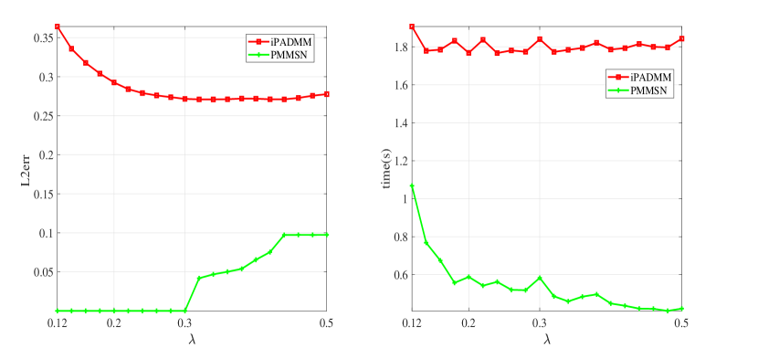
Figure 3: The relative $\ell_{2}$-error and computing time of two solvers under different $\lambda$

Figure 3 plots the relative $\ell_{2}$-error and computing time curves of two solvers under different $\lambda$, where iPADMM is solving (27) with $\varepsilon_{\rm opt}=0.7$. We see that as the parameter $\lambda$ increases, the relative $\ell_{2}$-error of iPADMM first decreases and then increases slightly, whereas the relative $\ell_{2}$-error of PMMSN has a remarkable increase after $\lambda>0.3$ but is still much lower than that of iPADMM. This means that if the sparsity of the noise $\varpi$ is well controlled, the increase of $\lambda$ in a certain range has a small influence on the error bound of the output of PMMSN. In addition, as $\lambda$ increases, the time of iPADMM has a tiny change, but the time of PMMSN becomes less and is always less than that of iPADMM. This shows that PMMSN has a better performance for this class of noise.

3. Performance of two solvers for other sparse noises

We test the performance of two solvers for other types of sparse noises via six examples, generated randomly with $p=5000,s^{*}=\lfloor\sqrt{p}/2\rfloor$ and $n=\lfloor 2s^{*}\ln(p)\rfloor$. The sparsity of the noise vector $\varpi$ is always set as $|\mathcal{I}|=\lfloor 0.3n\rfloor$ and the nonzero entries of $x^{*}$ follow $N(0,4)$. The covariance matrix $\Sigma$ includes the autoregressive structure $\Sigma=(0.5^{|i-j|})_{ij}$ denoted by ${\rm AR}_{0.5}$ and the compound symmetric structure $\Sigma=(\alpha+(1\!-\!\alpha)\mathbb{I}_{\{i=j\}})$ for $\alpha=0.6$, denoted by ${\rm CS}_{0.6}$. Such covariance matrices are highly relevant although they are positive definite. The nonzero entries of $\varpi$ obey the following distributions: (1) the normal distribution $N(0,100)$; (2) the scaled Student’s $t$-distribution with $4$ degrees of freedom $\sqrt{2}\times t_{4}$; (3) the mixture normal distribution $N(0,\sigma^{2})$ with $\sigma\sim{\rm Unif}(1,5)$, denoted by ${\rm MN}$; (4) the Laplace distribution with density $d(u)=0.5\exp(-|u|)$; and (5) the Cauchy distribution with density $d(u)=\frac{1}{\pi(1+u^{2})}$. Table 1 reports the average of the loss values, relative $\ell_{2}$-errors and computing time of total 10 test problems for each example with a fixed $\lambda$, for which we always take $\lambda=\max(0.05,0.12n^{-1}\!\interleave\!A\interleave_{1})$ by the assumption on $\lambda$ in Theorem 4.3. In Table 1, a$=$iPADMM and b$=$PMMSN, $\textbf{Nz}=N_{\rm nz}(x^{\rm out})$ denotes the approximate zero-norm of $x^{\rm out}$, Loss means the loss value $\frac{1}{n}\|Ax^{\rm out}\!-b\|_{1}$, $\|A\|^{2}$ means the average of the square spectral norm of $A$ for $10$ test problems, ${\bf FP}$ and ${\bf FN}$ respectively represents the number of false positives and false zeros of $x^{\rm out}$, and $\varepsilon$ column lists the interval to search the best $\varepsilon_{\rm opt}$. During the testing, we find that when $\Sigma$ takes ${\rm CS}_{0.6}$, the noise of Cauchy distribution will have a norm over $10^{3}$, for which the two solvers both fail to yielding a reasonable solution. In view of this, we choose the 10 test problems generated randomly with $\|\varpi\|_{\infty}<1000$ for testing.

Table 1: The performance of iPADMM and PMMSN for sparse noise

Problem	$\|A\|^{2}$	$\varepsilon$	$\varepsilon_{\rm opt}$	$\|\varpi\|_{\infty}$	Nz	Loss	L2err	FP	FN	Time(s)
$\Sigma$|$\varpi$					$a|b$	$a|b$	$a|b$	$a|b$	$a|b$	$a|b$
${\rm AR}_{0.5}$|$N(0,100)$	1.08e+4	[15,30]	25	9.90	38.1|35.0	1.501|1.489	2.34e-3|5.68e-7	3.2|0	0.1|0	42.4|45.9
${\rm AR}_{0.5}$|$\sqrt{2}\times t_{4}$	1.08e+4	[10,30]	15	12.4	39.6|35.0	0.464|0.448	3.01e-3|2.21e-6	4.7|0	0.1|0	44.5|42.3
${\rm AR}_{0.5}$|MN	1.08e+4	[10,30]	20	12.07	36.2|35.0	0.734|0.725	1.73e-3 |1.68e-6	1.3|0	0.1|0	46.7|53.5
${\rm AR}_{0.5}$|Laplace	1.08e+4	[10,30]	15	6.32	35.7|35.0	0.301|0.294	1.18e-3|8.21e-6	0.8|0	0.1|0	43.8|49.8
${\rm AR}_{0.5}$|Cauchy	1.08e+4	[20,35]	27	322.7	90.5|34.0	2.208|1.477	2.81e-1|9.96e-3	60.3|0	4.8|1	42.1|108.5
${\rm CS}_{0.6}$|$N(0,100)$	1.77e+6	[1600,2000]	1800	9.90	34.5|34.8	2.907|1.504	3.59e-1|4.54e-3	11.6|0.1	12.1|0.3	50.6|28.6
${\rm CS}_{0.6}$|$\sqrt{2}\times t_{4}$	1.77e+6	[1000,1500]	1225	12.4	39.3|34.9	1.571|0.462	2.44e-1|4.07e-3	12.1|0	7.8|0.1	50.4|19.5
${\rm CS}_{0.6}$|MN	1.77e+6	[1000,1500]	1350	12.07	39.5|34.6	1.968|0.753	2.84e-1|8.19e-3	13.2|0	8.7|0.4	59.5|24.9
${\rm CS}_{0.6}$|Laplace	1.77e+6	[1000,1500]	1150	6.32	36.3|35.1	1.341|0.302	2.15e-1|2.24e-3	8.6|0.2	7.3|0.1	60.2|22.5
${\rm CS}_{0.6}$|Cauchy	1.80e+6	[1200,1800]	1500	322.7	226.7|29.4	3.523|1.828	9.35e-1|9.28e-2	209.3|0.2	17.6|5.8	51.1|93.8

From Table 1, we see that the average sparsity yielded by PMMSN and iPADMM for all test examples except for ${\rm AR}_{0.5}$|Cauchy and ${\rm CS}_{0.6}$|Cauchy is close to that of the true vector $x^{*}$, but the average relative $\ell_{2}$-error and $({\bf FP},{\bf FN})$ yielded by iPADMM are worse than those yielded by PMMSN, especially for those examples of ${\rm CS}_{0.6}$. For the most difficult ${\rm CS}_{0.6}$|Cauchy, the average sparsity, relative $\ell_{2}$-error and $({\bf FP},{\bf FN})$ given by iPADMM are much worse than those yielded by PMMSN since, the parameter $\varepsilon$ is very sensitive to the data and the best $\varepsilon_{\rm opt}$ is not suitable for all $10$ test problems. This shows that replacing $f$ with a smooth approximation $e_{\varepsilon}f$ is not effective for highly relevant covariance matrix $\Sigma$ and heavy-tailed sparse noises, though $\varepsilon$ is elaborately selected.

5.3.2 Real data examples

This part uses the LIBSVM datasets from https://www.csie.ntu.edu.tw to test the efficiency of PMMSN for large scale problems. For those data sets with a few features, such as pyrim, abalone, bodyfat, housing, mpg, space ga, we follow the same line as in [39] to expand their original features by using polynomial basis functions over those features. For example, the last digit in pyrim5 indicates that a polynomial of order $5$ is used to generate the basis function. Such a naming convention is also applicable to the other expanded data sets. These data sets are quite difficult in terms of the dimension and the largest eigenvalues of $A^{\mathbb{T}}A$. Table 2 reports the numerical results of two solvers to solve the corresponding problems with $\lambda=\max(0.05,0.1n^{-1}\!\interleave\!A\interleave_{1})$.

Table 2: The performance of two solvers for LIBSVM datasets

Name of data	$(n,p)$	$\|A\|^{2}$	$\lambda$	$\varepsilon$	$\varepsilon_{\rm opt}$	NZ	Loss	Time(s)
						$a|b$	$a|b$	$a|b$
E2006.test	3308;150358	4.79e+4	0.3776	[0.1,10]	2.5	1|1	0.2361|0.2361	42|42
log1p.E2006.test	3308;4272226	1.46e+7	0.5395	[1500,2500]	2000	1|1	0.2362|0.2361	7071|3208
abalone7	4177;6435	5.23e+5	0.1	[500,1500]	1250	28|20	1.5140|1.4800	433|165
bodyfat7	252;116280	5.30e+4	0.1	[0.1,1]	0.3	3|3	7.45e-4|4.50e-4	604|466
housing7	506;77520	3.28e+5	0.1	[200,600]	470	137 |139	2.6596|1.0204	791|604
mpg7	392;3432	1.30e+4	0.1	[50,150]	90	$15|15$	$1.9826|1.7744$	$20|4$
pyrim5	74;201376	1.22e+6	0.1	[15,150]	60	$21|21$	$0.0783|0.0185$	$349|210$
space ga9	3107;5005	4.10e+3	0.1	[0.1,10]	5	$5|5$	$0.1040|0.0982$	$261|127$

From Table 2, PMMSN works well in solving large scale difficult problems. Although the sparsity of its output is very close to that of the output of iPADMM, the loss value of its output is lower than that of the output of iPADMM. From the numerical tests for synthetic example, the loss value is usually consistent with the relative error. This means that the output yielded by PMMSN has better quality. In particular, the computing time required by PMMSN is less than the time required by iPADMM.

From the above numerical comparisons, we conclude that PMMSN has an advantage in the quality of solutions and computing time, and it is robust under the scenario where $a_{i}^{\mathbb{T}}$ has a highly-relevant covariance and the noise is heavily-tailed, while the performance of iPADMM depends much on the smoothing parameter $\varepsilon$, and for those tough examples, the parameter $\varepsilon$ is very sensitive to the data. In addition, from the numerical results on synthetic examples, we find that when the sparsity of the noise $\varpi$ attains a certain level, say, $|\mathcal{I}|\leq 0.6n$ for Example 5.1 and $|\mathcal{I}|\leq 0.3n$ for Example 5.2 and the first fourth examples in Table 1, the relative $\ell_{2}$-error has an order about $10^{-6}$ which is close to the exact recovery. Then, it is natural to ask for which kind of covariance matrix $\Sigma$ and noises, the exact recovery of the limit $\overline{x}$ can be achieved by controlling the sparsity of the noise vector $\varpi$. We leave this interesting question for a future research topic.

6 Conclusions

For the zero-norm regularized PLQ composite problem, we have shown that its equivalent MPEC is partially calm over the set of global optima and obtain a family of equivalent DC surrogates by using this important property, which greatly improves the result of [27, Theorem 3.2] for this class of problems. We develop a proximal MM method for solving one of the DC surrogates, and provide its theoretical certificates by establishing its global and local linear convergence, analyzing when the limit of the generated sequence is a local minimum, and deriving the error bound of the limit to the true vector for the data $(b,A)$ from a linear observation model. Numerical comparisons with the convergent iPADMM for synthetic and real data examples verify that the proximal MM method armed with a dual semismooth Newton method for solving the subproblems has an advantage in the quality of solutions and the computing time, and is robust for the case where $A$ has a large spectral norm and $b$ is corrupted by the heavily-tailed noise; whereas the convergent iPADMM for the partially smoothed surrogate is ineffective for those tough test examples even with an elaborate selection of the smoothing parameter $\varepsilon$.

Acknowledgements  The authors would like to express their sincere thanks to Prof. Kim-Chuan Toh from National University of Singapore for helpful suggestions on the implementation of Algorithm 3 when visiting SCUT in March of 2019, and give thanks to Prof. Liping Zhu from RenMin University of China for helpful discussion on the result of Theorem 4.3. The research of Shaohua Pan and Shujun Bi is supported by the National Natural Science Foundation of China under project No.11971177 and No.11701186.

Appendix A

Lemma 1

Fix any $x\in\mathbb{R}^{p}$ and $\rho>0$. Let $w_{\rho}\!:\mathbb{R}^{p}\to\mathbb{R}^{p}$ be the mapping in (13b). Then,

$$\nabla g_{\rho}(x)=w_{\rho}(x)\circ{\rm sign}(x)\quad\ \forall x\in\mathbb{R}^{p}.$$

Proof: By the expressions of $g_{\rho}$ and $w_{\rho}$ in equation (13a)-(13b), it suffices to argue that $\rho^{-1}\varphi_{\rho}^{\prime}(x_{i})\!=\!(\psi^{*})^{\prime}(\rho|x_{i}|){\rm sign}(x_{i})$ for each $i$. By the expression of $\psi^{*}$, for any $t\in\mathbb{R}$,

$$\varphi_{\rho}^{\prime}(t)=\left\{\begin{array}[]{cl}0&\textrm{if}\ |t|\leq\frac{2}{\rho(a+1)};\\ \frac{\rho((a+1)\rho|t|-2){\rm sign}(t)}{2(a-1)}&\textrm{if}\ \frac{2}{\rho(a+1)}<|t|\leq\frac{2a}{\rho(a+1)};\\ \rho{\rm sign}(t)&\textrm{if}\ |t|>\frac{2a}{\rho(a+1)}.\end{array}\right.$$ (34)

On the other hand, by the expression of $\psi^{*}$ in (12), it is easy to check that

$$(\psi^{*})^{\prime}(\rho|x_{i}|){\rm sign}(x_{i})=\left\{\begin{array}[]{cl}0&\textrm{if}\ |x_{i}|\leq\frac{2}{\rho(a+1)},\\ \frac{(\rho(a+1)|x_{i}|-2){\rm sign}(x_{i})}{2(a-1)}&\textrm{if}\ \frac{2}{\rho(a+1)}<|x_{i}|\leq\frac{2a}{\rho(a+1)},\\ {\rm sign}(x_{i})&\textrm{if}\ |x_{i}|>\frac{2a}{\rho(a+1)}.\end{array}\right.$$

By comparing $\rho^{-1}\varphi_{\rho}^{\prime}(x_{i})$ with $(\psi^{*})^{\prime}(\rho|x_{i}|){\rm sign}(x_{i})$, the stated equality holds. $\Box$

Proof of Proposition 3.2 (i) The lower boundedness and coerciveness of $\Theta_{\lambda,\rho}$ follows by the expressions of $\psi^{*}$ and the lower boundedness on $f$. By equation (34), a simple calculation shows $\varphi_{\rho}^{\prime}$ is Lipschitz continuous in $\mathbb{R}$ of modulus $\rho^{2}\max(\frac{a+1}{2},\frac{a+1}{2(a-1)})$. Notice that $g_{\rho}(x)=\rho^{-1}\sum_{i=1}^{p}\varphi_{\rho}(x_{i})$. Then, $-\nabla g_{\rho}$ is globally Lipschitz on $\mathbb{R}^{p}$ with the same Lip-constant. By invoking the descent lemma, this means that $-g_{\rho}$ is semiconvex of modulus $\rho^{2}\max(\frac{a+1}{2},\frac{a+1}{2(a-1)})$ and so is the function $\Theta_{\lambda,\rho}$.

(ii) Since $\Theta_{\lambda,\rho}$ is semiconvex, the first two equalities follow by Remark 2.1(iii). By using the smoothness of $g_{\rho}$ and [35, Exercise 8.9], it follows that

$$\partial\Theta_{\lambda,\rho}(x)=\partial(F_{\mu}(\cdot)+\lambda\|\cdot\|_{1}+\delta_{\Omega}(\cdot))(x)-\lambda\nabla g_{\rho}(x).$$

In addition, since ${\rm dom}f=\mathbb{R}^{p}$, from [33, Theorem 23.8] it follows that

$$\partial(F_{\mu}(\cdot)+\lambda\|\cdot\|_{1}+\delta_{\Omega}(\cdot))(x)=A^{\mathbb{T}}\partial\!f(Ax\!-b)+\mu x+\lambda\partial\|x\|_{1}+\mathcal{N}_{\Omega}(x).$$

The result directly follows from the last two equations.

(iii) Since $x\in\mathbb{R}^{p}$ is a critical point of $\Theta_{\lambda,\rho}$, from part (ii) and Lemma 1 it follows that

$$0 \in A^{\mathbb{T}}\partial\!f(Ax\!-b)+\mu x+\mathcal{N}_{\Omega}(x)+\lambda\partial\|x\|_{1}-\lambda\nabla g_{\rho}(x)$$

$$=A^{\mathbb{T}}\partial\!f(Ax\!-b)+\mu x+\mathcal{N}_{\Omega}(x)+\lambda\big{[}(1\!-\![w_{\rho}(x)]_{1})\partial|x_{1}|\times\cdots\times(1\!-\![w_{\rho}(x)]_{p})\partial|x_{p}|\big{]}$$

where $w_{\rho}\!:\mathbb{R}^{p}\to\mathbb{R}^{p}$ is the mapping defined in equation (13b), and the equality is using the fact that $[w_{\rho}(x)]_{i}=0$ if $x_{i}=0$ and $\partial|x_{i}|=\{{\rm sign}(x_{i})\}$ if $x_{i}\neq 0$. Notice that $[w_{\rho}(x)]_{i}=(\psi^{*})^{\prime}(\rho|x_{i}|)=\min\big{[}1,\max\big{(}0,\frac{(a+1)\rho|x_{i}|-2}{2(a-1)}\big{)}\big{]}$ for each $i$. Since $|x_{\rm nz}|\geq\frac{2a}{\rho(a+1)}$ by the given assumption, we have $[w_{\rho}(x)]_{i}=1$ for all $i\in{\rm supp}(x)$. Combining this with the last equation and the subdifferential characterization of $\|\cdot\|_{0}$ in [19], we conclude that

$$0\in A^{\mathbb{T}}\partial\!f(Ax\!-b)+\mu x+\mathcal{N}_{\Omega}(x)+\partial\|x\|_{0}.$$

The right hand side of the last inclusion is exactly the regular subdifferential of the objective function of (1). Thus, $x$ is a regular critical point of (1).

(iv) Since the set $\Omega$ is polyhedral and the function $F_{\mu}+g_{\rho}$ is continuous and piecewise linear-quadratic, it follows that $\Theta_{\lambda,\rho}=F_{\mu}+g_{\rho}+\delta_{\Omega}$ is a piecewise linear-quadratic function with ${\rm dom}\Theta_{\lambda,\rho}=\Omega$. By [35, Definition 10.20], there exist $p\times p$ symmetric matrices $M^{1},\ldots,M^{m}$, vectors $b^{1},\ldots,b^{m}\in\mathbb{R}^{p}$ and scalars $c_{1},\ldots,c_{m}$ such that

$$\Theta_{\lambda,\rho}(z)=\min_{1\leq i\leq m}\!\Big{\{}\langle z,M^{i}z\rangle+\langle b^{i},z\rangle+c_{i}+\delta_{\mathcal{P}_{i}}(z)\Big{\}}\quad\ \forall z\in\mathbb{R}^{p}$$

where each $\mathcal{P}_{i}$ is a polyhedral set. Notice that $\delta_{\Omega}$ is continuous on the set $\Omega$ by the convexity of $\Omega$ and ${\rm ri}({\rm dom}\,\delta_{\Omega})=\Omega$. This means that $\Theta_{\lambda,\rho}=F_{\mu}+g_{\rho}+\delta_{\Omega}$ is continuous on the set $\Omega$. In addition, by Proposition 3.2(ii), we know that ${\rm dom}\partial\Theta_{\lambda,\rho}\subseteq\Omega$. The two sides show that $\Theta_{\lambda,\rho}$ is continuous on ${\rm dom}\partial\Theta_{\lambda,\rho}$. Now by invoking [23, Corollary 5.2] and the last equation, we obtain the desired result. The proof is then completed. $\Box$

Appendix B

Lemma 2

Let $\theta\!:\mathbb{R}^{n}\to\mathbb{R}_{+}$ be a convex function with $\theta(0)=0$. For any given $\overline{t}\in\mathbb{R}$,

$$\partial(\theta^{2})(\overline{t})=\left\{\begin{array}[]{cl}\{0\}&{\rm if}\ \theta(\overline{t})=0;\\ \theta(\overline{t})\partial\theta(\overline{t})&{\rm otherwise}.\end{array}\right.$$

Proof: By [35, Theorem 10.49], we have $\partial(\theta^{2})(\overline{t})=D^{*}\theta(\overline{t})(\theta(\overline{t}))$ where $D^{*}\theta(\overline{t})\!:\mathbb{R}\rightrightarrows\mathbb{R}$ denotes the coderivative of the function $\theta^{2}$ at $\overline{t}$. From [35, Proposition 9.24(b)], it follows that $D^{*}\theta(\overline{t})(\theta(\overline{t}))=\partial(\theta(\overline{t})\theta)(\overline{t}),$ which implies the desired result. $\Box$

In order to complete the proof of Theorem 4.3, we introduce the following notation

$$v^{k}\!:=e-w^{k},\ z^{k}\!:=Ax^{k}\!-b,\ \Delta x^{k}:=x^{k}-x^{*}\quad\ \forall k\in\mathbb{N};$$ (35a)

$$\xi^{k}\!:=(\gamma_{1,k-1}I+\gamma_{2,k-1}A^{\mathbb{T}}A)(x^{k-1}\!-x^{k})-\mu x^{*}\quad\ \forall k\in\mathbb{N}.$$ (35b)

With these notation, we can establish the following important technical lemma.

Lemma 3

Suppose for some $k\geq 1$ there exists $S^{k-1}\supseteq S^{*}$ with $\max_{i\in(S^{k-1})^{c}}w_{i}^{k-1}\leq\frac{1}{2}.$ Then, when $\lambda\geq 8n^{-1}\!\interleave\!A_{\mathcal{I}\cdot}\!\interleave_{1}+8\|\xi^{k}\|_{\infty}$, it holds that $\big{\|}\Delta x^{k}_{(S^{k-1})^{c}}\|_{1}\leq 3\|\Delta x^{k}_{S^{k-1}}\|_{1}$.

Proof: Since $x^{*}$ is a feasible solution and $x^{k}$ is an optimal one to (16), respectively, from the strong convexity of the objective function of (16), it follows that

$$f(\!Ax^{*}\!-\!b)+\lambda\langle v^{k-1},|x^{*}|\rangle+\frac{\mu}{2}\|x^{*}\|^{2}+\frac{\gamma_{1,k-1}}{2}\|x^{*}\!-\!x^{k-1}\|^{2}+\frac{\gamma_{2,k-1}}{2}\|A(x^{*}\!-\!x^{k-1})\|^{2}$$

$$\geq f(\!Ax^{k}\!-\!b)+\lambda\langle v^{k-1},|x^{k}|\rangle+\frac{\mu}{2}\|x^{k}\|^{2}+\frac{\gamma_{1,k-1}}{2}\|x^{k}\!-\!x^{k-1}\|^{2}+\frac{\gamma_{2,k-1}}{2}\|A(x^{k}\!-\!x^{k-1})\|^{2}$$

$$\quad+\frac{1}{2}\langle x^{*}\!-x^{k},(\mu I+\gamma_{1,k}I+\gamma_{2,k}A^{\mathbb{T}}A)(x^{*}\!-x^{k})\rangle,$$

which by $\frac{\mu}{2}\big{[}\|x^{k}\|^{2}-\|x^{*}\|^{2}\big{]}=\frac{\mu}{2}\|x^{k}\!-\!x^{*}\|^{2}+\mu\langle x^{k}\!-x^{*},x^{*}\rangle$ is equivalent to saying that

$$f(Ax^{k}\!-b)-f(Ax^{*}\!-b)+\mu\|\Delta x^{k}\|^{2}$$

$$\leq\lambda\langle v^{k-1},|x^{*}|-|x^{k}|\rangle+\gamma_{1,k-1}\langle x^{k-1}\!-\!x^{k},x^{k}\!-x^{*}\rangle$$

$$\quad+\gamma_{2,k-1}\langle A^{\mathbb{T}}A(x^{k-1}\!-\!x^{k}),x^{k}\!-x^{*}\rangle+\langle x^{*}\!-x^{k},\mu x^{*}\rangle$$

$$=\lambda\langle v^{k-1},|x^{*}|-|x^{k}|\rangle+\langle\xi^{k},x^{k}\!-x^{*}\rangle$$ (36)

where the equality is due to the definition of $\xi^{k}$. By using $\theta(0)=0$ and equation (25),

$$\theta(z_{i})\leq\widetilde{\tau}\|z\|_{\infty}\ \ {\rm for}\ \ i=1,\ldots,n\quad\ \forall z\in\mathbb{R}^{n}.$$ (37)

Recall $0\neq\varpi=b-Ax^{*}$ and the definition of the index set $\mathcal{I}$. For each $k\in\mathbb{N}$, define $\mathcal{J}_{k}:=\big{\{}i\notin\mathcal{I}\!:z_{i}^{k}\neq 0\big{\}}$. Then, together with the expression of $f$ and (37), we have

$$f(Ax^{k}\!-b)-f(Ax^{*}\!-b) =\frac{1}{n}\bigg{[}\sum_{i\in\mathcal{J}_{k}}\frac{\theta^{2}(z^{k}_{i})-\theta^{2}(\varpi_{i})}{\theta(z^{k}_{i})+\theta(\varpi_{i})}+\sum_{i\in\mathcal{I}}\frac{\theta^{2}(z^{k}_{i})-\theta^{2}(\varpi_{i})}{\theta(z^{k}_{i})+\theta(\varpi_{i})}\bigg{]}$$

$$\geq\frac{1}{n}\bigg{[}\sum_{i\in\mathcal{J}_{k}}\frac{\theta^{2}(z^{k}_{i})-\theta^{2}(\varpi_{i})}{\widetilde{\tau}\|z^{k}\|_{\infty}}+\sum_{i\in\mathcal{I}}\frac{\theta^{2}(z^{k}_{i})-\theta^{2}(\varpi_{i})}{\theta(z^{k}_{i})+\theta(\varpi_{i})}\bigg{]}.$$ (38)

Fix an arbitrary $\eta_{i}\in\partial(\theta^{2})(\varpi_{i})$. Since $\theta^{2}$ is strongly convex of modulus $\tau$, it holds that

$$\theta^{2}(z^{k}_{i})-\theta^{2}(\varpi_{i})\geq\eta_{i}(z_{i}^{k}-\varpi_{i})+0.5\tau(z^{k}_{i}-\varpi_{i})^{2}\ \ {\rm for}\ \ i=1,\ldots,n.$$ (39)

This by Lemma 2 implies that $\theta^{2}(z^{k}_{i})-\theta^{2}(\varpi_{i})\geq\frac{\tau}{2}(z^{k}_{i}-\varpi_{i})^{2}$ for each $i\in\mathcal{J}_{k}$, and hence

$$\sum_{i\in\mathcal{J}_{k}}\frac{\theta^{2}(z^{k}_{i})-\theta^{2}(\varpi_{i})}{\widetilde{\tau}\|z^{k}\|_{\infty}}\geq\frac{\tau}{2\widetilde{\tau}}\sum_{i\in\mathcal{J}_{k}}\frac{(z^{k}_{i}-\varpi_{i})^{2}}{\|z^{k}\|_{\infty}}.$$ (40)

For each $i\in\mathcal{I}$, write $\widetilde{z}_{i}^{k}=\frac{\eta_{i}}{\theta(z_{i}^{k})+\theta(\varpi_{i})}$. By Lemma 2, clearly, $0\leq\widetilde{z}_{i}^{k}\leq 1$ for each $i\in\mathcal{I}$. Together with the inequality (39), it immediately follows that

$$\sum_{i\in\mathcal{I}}\frac{\theta^{2}(z^{k}_{i})-\theta^{2}(\varpi_{i})}{\theta(z^{k}_{i})+\theta(\varpi_{i})} \geq\sum_{i\in\mathcal{I}}\widetilde{z}_{i}^{k}(z_{i}^{k}-\varpi_{i})+\frac{\tau}{2}\sum_{i\in\mathcal{I}}\frac{(z^{k}_{i}-\varpi_{i})^{2}}{\theta(z^{k}_{i})+\theta(\varpi_{i})}$$

$$\geq-\|\widetilde{z}^{k}\|_{\infty}\|[A(x^{k}\!-x^{*})]_{\mathcal{I}}\|_{1}+\frac{\tau}{2}\sum_{i\in\mathcal{I}}\frac{(z^{k}_{i}-\varpi_{i})^{2}}{\widetilde{\tau}(\|z^{k}\|_{\infty}+\|\varpi\|_{\infty})}$$

$$\geq-\big{\|}[A(x^{k}\!-x^{*})]_{\mathcal{I}}\big{\|}_{1}+\frac{\tau}{2\widetilde{\tau}}\sum_{i\in\mathcal{I}}\frac{(z^{k}_{i}-\varpi_{i})^{2}}{\|z^{k}\|_{\infty}+\|\varpi\|_{\infty}}$$ (41)

where the second inequality is due to (37). Substituting (40)-(A proximal MM method for the zero-norm regularized PLQ composite optimization problem) into (A proximal MM method for the zero-norm regularized PLQ composite optimization problem) yields that

$$f(Ax^{k}\!-b)-f(Ax^{*}\!-b) \geq-\frac{1}{n}\|[A(x^{k}\!-x^{*})]_{\mathcal{I}}\|_{1}+\frac{\tau}{2n\widetilde{\tau}}\sum_{i\in\mathcal{J}_{k}\cup\mathcal{I}}\frac{(z^{k}_{i}-\varpi_{i})^{2}}{\|z^{k}\|_{\infty}\!+\!\|\varpi\|_{\infty}}$$

$$=-\frac{1}{n}\|[A(x^{k}\!-x^{*})]_{\mathcal{I}}\|_{1}+\frac{\tau\|A(x^{k}\!-x^{*})\|^{2}}{2n\widetilde{\tau}(\|z^{k}\|_{\infty}\!+\!\|\varpi\|_{\infty})}.$$

By combining this inequality and the inequality (A proximal MM method for the zero-norm regularized PLQ composite optimization problem), it follows that

$$\mu\|\Delta x^{k}\|^{2}+\frac{\tau\|A(x^{k}-x^{*})\|^{2}}{2n\widetilde{\tau}(\|z^{k}\|_{\infty}\!+\!\|\varpi\|_{\infty})}$$

$$\leq\lambda\langle v^{k-1},|x^{*}|-|x^{k}|\rangle+\frac{1}{n}\big{\|}[A(x^{k}\!-x^{*})]_{\mathcal{I}}\big{\|}_{1}+\langle\xi^{k},x^{k}\!-x^{*}\rangle$$

$$\leq\lambda\langle v^{k-1},|x^{*}|-|x^{k}|\rangle+\big{(}n^{-1}\!\interleave\!A_{\mathcal{I}\cdot}\!\interleave_{1}+\|\xi^{k}\|_{\infty}\big{)}\big{\|}x^{k}\!-x^{*}\big{\|}_{1}$$

$$\leq\lambda\Big{(}\textstyle{\sum_{i\in S^{*}}}v_{i}^{k-1}|\Delta x_{i}^{k}|-\textstyle{\sum_{i\in(S^{k-1})^{c}}}v_{i}^{k-1}|\Delta x_{i}^{k}|\Big{)}$$

$$\quad\ +\big{(}n^{-1}\!\interleave\!A_{\mathcal{I}\cdot}\!\interleave_{1}+\|\xi^{k}\|_{\infty}\big{)}\big{(}\|\Delta x_{S^{k-1}}^{k}\|_{1}+\|\Delta x_{(S^{k-1})^{c}}^{k}\|_{1}\big{)}.$$ (42)

Since $S^{k-1}\supseteq S^{*}$ and $v_{i}^{k-1}\in[0.5,1]$ for $i\in(S^{k-1})^{c}$, from the last inequality we have

$$\mu\|\Delta x^{k}\|^{2}+\frac{\tau\|A(x^{k}\!-x^{*})\|^{2}}{2n\widetilde{\tau}(\|z^{k}\|_{\infty}\!+\!\|\varpi\|_{\infty})} \leq\textstyle{\sum_{i\in S^{k-1}}}\big{(}\lambda v_{i}^{k-1}+n^{-1}\!\interleave\!A_{\mathcal{I}\cdot}\!\interleave_{1}+\|\xi^{k}\|_{\infty}\big{)}\big{|}\Delta x_{i}^{k}\big{|}$$

$$\quad+\textstyle{\sum_{i\in(S^{k-1})^{c}}}\big{(}n^{-1}\!\interleave\!A_{\mathcal{I}\cdot}\!\interleave_{1}+\|\xi^{k}\|_{\infty}-\lambda/2\big{)}\big{|}\Delta x_{i}^{k}\big{|}$$

$$=\big{(}\lambda+n^{-1}\!\interleave\!A_{\mathcal{I}\cdot}\!\interleave_{1}+\|\xi^{k}\|_{\infty}\big{)}\big{\|}\Delta x_{S^{k-1}}^{k}\big{\|}_{1}$$

$$\quad+\big{(}n^{-1}\!\interleave\!A_{\mathcal{I}\cdot}\!\interleave_{1}+\|\xi^{k}\|_{\infty}-\lambda/2\big{)}\big{\|}\Delta x_{(S^{k-1})^{c}}^{k}\big{\|}_{1}.$$

From the nonnegativity of the left hand side and the given assumption on $\lambda$, we have

$$\big{\|}\Delta x_{(S^{k-1})^{c}}^{k}\big{\|}_{1}\leq\frac{\lambda+n^{-1}\!\interleave\!A_{\mathcal{I}\cdot}\!\interleave_{1}+\|\xi^{k}\|_{\infty}}{0.5\lambda-n^{-1}\!\interleave\!A_{\mathcal{I}\cdot}\!\interleave_{1}-\|\xi^{k}\|_{\infty}}\big{\|}\Delta x_{S^{k-1}}^{k}\big{\|}_{1}\leq 3\big{\|}\Delta x_{S^{k-1}}^{k}\big{\|}_{1}.$$

This implies that the desired result holds. The proof is completed. $\Box$

Now by using the inequality (A proximal MM method for the zero-norm regularized PLQ composite optimization problem) and Lemma 3, we obtain the following conclusion.

Lemma 4

Suppose that the matrix $A^{\mathbb{T}}A/n$ satisfies the RE condition of parameter $\kappa>0$ over $\mathcal{C}(S^{*})$ and for some $k\geq 1$ there exists an index set $S^{k-1}$ with $|S^{k-1}|\leq 1.5s^{*}$ such that $S^{k-1}\supseteq S^{*}$ and $\max_{i\in(S^{k-1})^{c}}w_{i}^{k-1}\leq\frac{1}{2}$. If the parameter $\lambda$ is chosen such that $8n^{-1}\!\interleave\!A_{\mathcal{I}\cdot}\!\interleave_{1}+8\|\xi^{k}\|_{\infty}\leq\lambda<\frac{2\mu\widetilde{\tau}\|\varpi\|_{\infty}+\tau\kappa-4\widetilde{\tau}\|A\|_{\infty}(n^{-1}\interleave A_{\mathcal{I}\cdot}\interleave_{1}+\|\xi^{k}\|_{\infty})|S^{k-1}|}{4\widetilde{\tau}\|A\|_{\infty}\|v_{S^{*}}^{k-1}\|_{\infty}|S^{k-1}|}$, then

$$\big{\|}\Delta x^{k}\big{\|}\leq\frac{2\widetilde{\tau}\|\varpi\|_{\infty}\big{(}\lambda\|v_{S^{*}}^{k-1}\|_{\infty}+n^{-1}\!\interleave\!A_{\mathcal{I}\cdot}\!\interleave_{1}+\|\xi^{k}\|_{\infty}\big{)}\sqrt{|S^{k-1}|}}{2\mu\widetilde{\tau}\|\varpi\|_{\infty}+\tau\kappa-4\widetilde{\tau}\|A\|_{\infty}\big{(}\lambda\|v_{S^{*}}^{k-1}\|_{\infty}+n^{-1}\!\interleave\!A_{\mathcal{I}\cdot}\!\interleave_{1}+\|\xi^{k}\|_{\infty}\big{)}|S^{k-1}|}.$$

Proof: Note that $\|z^{k}\|_{\infty}+\|\varpi\|_{\infty}=\|\varpi-\!A\Delta x^{k}\|_{\infty}+\|\varpi\|_{\infty}\leq\|A\Delta x^{k}\|_{\infty}+2\|\varpi\|_{\infty}$. So,

$$\frac{\tau\|A(x^{k}-x^{*})\|^{2}}{2n\widetilde{\tau}(\|z^{k}\|_{\infty}+\|\varpi\|_{\infty})}\geq\frac{\tau\|A\Delta x^{k}\|^{2}}{2n\widetilde{\tau}(\|A\Delta x^{k}\|_{\infty}+2\|\varpi\|_{\infty})}.$$

Together with the inequality (A proximal MM method for the zero-norm regularized PLQ composite optimization problem) and $v_{i}^{k-1}\in[0.5,1]$ for $i\in(S^{k-1})^{c}$, it follows that

$$\mu\|\Delta x^{k}\|^{2}+\frac{\tau\|A\Delta x^{k}\|^{2}}{2n\widetilde{\tau}(\|A\Delta x^{k}\|_{\infty}+2\|\varpi\|_{\infty})}$$

$$\leq\lambda{\textstyle\sum_{i\in S^{*}}}v_{i}^{k-1}|\Delta x_{i}^{k}|-({\lambda}/{2}){\textstyle\sum_{i\in(S^{k-1})^{c}}}|\Delta x_{i}^{k}|$$

$$\quad+\big{(}n^{-1}\!\interleave\!A_{\mathcal{I}\cdot}\!\interleave_{1}+\|\xi^{k}\|_{\infty}\big{)}\big{(}\|\Delta x_{S^{k-1}}^{k}\|_{1}+\|\Delta x_{(S^{k-1})^{c}}^{k}\|_{1}\big{)}$$

$$\leq\big{(}\lambda\|v_{S^{*}}^{k-1}\|_{\infty}+n^{-1}\!\interleave\!A_{\mathcal{I}\cdot}\!\interleave_{1}+\|\xi^{k}\|_{\infty}\big{)}\|\Delta x_{S^{k-1}}^{k}\|_{1}$$

where the last inequality is due to $\lambda\geq 8n^{-1}\!\interleave\!A_{\mathcal{I}\cdot}\!\interleave_{1}+8\|\xi^{k}\|_{\infty}$. By Lemma 3, we know that $\|\Delta x^{k}_{(S^{k-1})^{c}}\|_{1}\leq 3\|\Delta x^{k}_{S^{k-1}}\|_{1}$, which by the given assumption means that $\Delta x^{k}\in\mathcal{C}(S^{*})$. From the given assumption on $\frac{1}{n}A^{\mathbb{T}}A$, we have $\|A\Delta x^{k}\|^{2}\geq 2n\kappa\|\Delta x^{k}\|^{2}$. Then,

$$\mu\|\Delta x^{k}\|^{2}+\frac{\tau\kappa\|\Delta x^{k}\|^{2}}{\widetilde{\tau}(\|A\Delta x^{k}\|_{\infty}\!+2\|\varpi\|_{\infty})}\leq\Big{(}\lambda\|v_{S^{*}}^{k-1}\|_{\infty}+\frac{1}{n}\!\interleave\!A_{\mathcal{I}\cdot}\!\interleave_{1}+\|\xi^{k}\|_{\infty}\Big{)}\big{\|}\Delta x_{S^{k-1}}^{k}\big{\|}_{1}.$$

Multiplying the both sides of this inequality by $\widetilde{\tau}(\|A\Delta x^{k}\|_{\infty}+2\|\varpi\|_{\infty})$ yields that

$$\big{[}\mu\widetilde{\tau}(\|A\Delta x^{k}\|_{\infty}+2\|\varpi\|_{\infty})+\tau\kappa\big{]}\|\Delta x^{k}\|^{2}$$

$$\leq\widetilde{\tau}\big{(}\|A\Delta x^{k}\|_{\infty}+2\|\varpi\|_{\infty}\big{)}\big{(}\lambda\|v_{S^{*}}^{k-1}\|_{\infty}+n^{-1}\!\interleave\!A_{\mathcal{I}\cdot}\!\interleave_{1}+\|\xi^{k}\|_{\infty}\big{)}\big{\|}\Delta x_{S^{k-1}}^{k}\big{\|}_{1}$$

$$\leq\widetilde{\tau}\|A\Delta x^{k}\|_{\infty}\big{(}\lambda\|v_{S^{*}}^{k-1}\|_{\infty}+n^{-1}\!\interleave\!A_{\mathcal{I}\cdot}\!\interleave_{1}+\|\xi^{k}\|_{\infty}\big{)}\big{\|}\Delta x_{S^{k-1}}^{k}\big{\|}_{1}$$

$$\quad+2\widetilde{\tau}\|\varpi\|_{\infty}\big{(}\lambda\|v_{S^{*}}^{k-1}\|_{\infty}+n^{-1}\!\interleave\!A_{\mathcal{I}\cdot}\!\interleave_{1}+\|\xi^{k}\|_{\infty}\big{)}\big{\|}\Delta x_{S^{k-1}}^{k}\big{\|}_{1}.$$

Note that $\|A\Delta x^{k}\|_{\infty}\leq\|A\|_{\infty}\|\Delta x^{k}\|_{1}$. Along with $\|\Delta x^{k}_{(S^{k-1})^{c}}\|_{1}\leq 3\|\Delta x^{k}_{S^{k-1}}\|_{1}$, we have $\|A\Delta x^{k}\|_{\infty}\leq 4\|A\|_{\infty}\|\Delta x_{S^{k-1}}^{k}\|_{1}$. So, the right hand side of the last inequality satisfies

$${\rm RHS} \leq 4\widetilde{\tau}\|A\|_{\infty}\big{(}\lambda\|v_{S^{*}}^{k-1}\|_{\infty}+n^{-1}\!\interleave\!A_{\mathcal{I}\cdot}\!\interleave_{1}+\|\xi^{k}\|_{\infty}\big{)}\big{\|}\Delta x_{S^{k-1}}^{k}\big{\|}_{1}^{2}$$

$$\quad+2\widetilde{\tau}\|\varpi\|_{\infty}\big{(}\lambda\|v_{S^{*}}^{k-1}\|_{\infty}+n^{-1}\!\interleave\!A_{\mathcal{I}\cdot}\!\interleave_{1}+\|\xi^{k}\|_{\infty}\big{)}\big{\|}\Delta x_{S^{k-1}}^{k}\big{\|}_{1}$$

$$\leq 4\widetilde{\tau}\|A\|_{\infty}\big{(}\lambda\|v_{S^{*}}^{k-1}\|_{\infty}+n^{-1}\!\interleave\!A_{\mathcal{I}\cdot}\!\interleave_{1}+\|\xi^{k}\|_{\infty}\big{)}|S^{k-1}|\big{\|}\Delta x_{S^{k-1}}^{k}\big{\|}^{2}$$

$$\quad+2\widetilde{\tau}\|\varpi\|_{\infty}\big{(}\lambda\|v_{S^{*}}^{k-1}\|_{\infty}+n^{-1}\!\interleave\!A_{\mathcal{I}\cdot}\!\interleave_{1}+\|\xi^{k}\|_{\infty}\big{)}\sqrt{|S^{k-1}|}\big{\|}\Delta x_{S^{k-1}}^{k}\big{\|}.$$

From the last two equations, a suitable rearrangement yields that

$$\Big{[}2\mu\widetilde{\tau}\|\varpi\|_{\infty}+\tau\kappa-4\widetilde{\tau}\|A\|_{\infty}\big{(}\lambda\|v_{S^{*}}^{k-1}\|_{\infty}+n^{-1}\!\interleave\!A_{\mathcal{I}\cdot}\!\interleave_{1}+\|\xi^{k}\|_{\infty}\big{)}|S^{k-1}|\Big{]}\|\Delta x^{k}\|^{2}$$

$$\leq 2\widetilde{\tau}\|\varpi\|_{\infty}\big{(}\lambda\|v_{S^{*}}^{k-1}\|_{\infty}+n^{-1}\!\interleave\!A_{\mathcal{I}\cdot}\!\interleave_{1}+\|\xi^{k}\|_{\infty}\big{)}\sqrt{|S^{k-1}|}\big{\|}\Delta x_{S^{k-1}}^{k}\big{\|},$$

which by $\lambda<\frac{2\mu\widetilde{\tau}\|\varpi\|_{\infty}+\tau\kappa-4\widetilde{\tau}\|A\|_{\infty}(n^{-1}\interleave A_{\mathcal{I}\cdot}\interleave_{1}+\|\xi^{k}\|_{\infty})|S^{k-1}|}{4\widetilde{\tau}\|A\|_{\infty}\|v_{S^{*}}^{k-1}\|_{\infty}|S^{k-1}|}$ implies the desired result. $\Box$

Proof of Theorem 4.3: Since $x^{k}\to\overline{x}$ as $k\to\infty$ and $\gamma_{1,k}\geq\underline{\gamma_{1}}$ and $\gamma_{2,k}\geq\underline{\gamma_{2}}$, by the definition of $\xi^{k}$ in (35b), we have $\xi^{k}\to\mu x^{*}$. So, there exists $\widehat{k}\in\mathbb{N}$ such that $\|\xi^{k}\|_{\infty}\leq\frac{3}{2}\mu\|x^{*}\|_{\infty}$ for all $k\geq\overline{k}$. Since $x^{k}\to\overline{x}$, there is $\widetilde{k}\in\mathbb{N}$ such that for all $k\geq\widetilde{k}$,

$$|x_{i}^{k}|-|\overline{x}_{i}|\leq|x_{i}^{k}-\overline{x}_{i}|\leq\frac{1}{\rho(a+1)}\ \ {\rm for}\ i=1,2,\ldots,n.$$

This, by the assumption on $\overline{x}$, implies that $|x_{i}^{k}|\leq\frac{1}{\rho}$ for $i\notin S^{*}$, and from (17) we have $w_{i}^{k}\in[0,1/2]$ for each $i\in(S^{*})^{c}$ when $k\geq\widetilde{k}$. Set $\overline{k}:=\max(\widehat{k},\widetilde{k})$ and for each $k$ define $S^{k-1}:=S^{*}\cup\{i\notin S^{*}\!:w^{k-1}_{i}>\frac{1}{2}\}$. If $|S^{k-1}|\leq 1.5s^{*}$ for $k\geq\overline{k}$, from Lemma 4 we have

$$\big{\|}x^{k}\!-x^{*}\big{\|} \leq\frac{2\widetilde{\tau}\big{(}\lambda\|v_{S^{*}}^{k-1}\|_{\infty}+n^{-1}\!\interleave\!A_{\mathcal{I}\cdot}\!\interleave_{1}+\frac{3}{2}\mu\|x^{*}\|_{\infty}\big{)}\sqrt{|S^{k-1}|}\|\varpi\|_{\infty}}{2\mu\widetilde{\tau}\|\varpi\|_{\infty}+\tau\kappa-4\widetilde{\tau}\|A\|_{\infty}\big{(}\lambda\|v_{S^{*}}^{k-1}\|_{\infty}+n^{-1}\!\interleave\!A_{\mathcal{I}\cdot}\!\interleave_{1}+\frac{3}{2}\mu\|x^{*}\|_{\infty}\big{)}|S^{k-1}|}$$

$$\leq\frac{2\widetilde{\tau}\big{(}\lambda\|v_{S^{*}}^{k-1}\|_{\infty}+n^{-1}\!\interleave\!A_{\mathcal{I}\cdot}\!\interleave_{1}+\frac{3}{2}\mu\|x^{*}\|_{\infty}\big{)}\sqrt{|S^{k-1}|}\|\varpi\|_{\infty}}{2\mu\widetilde{\tau}\|\varpi\|_{\infty}+\tau\kappa-4\widetilde{\tau}\|A\|_{\infty}\big{(}\lambda\|v_{S^{*}}^{k-1}\|_{\infty}+n^{-1}\!\interleave\!A_{\mathcal{I}\cdot}\!\interleave_{1}+\frac{3}{2}\mu\|x^{*}\|_{\infty}\big{)}\sqrt{1.5s^{*}}}$$

$$\leq c\widetilde{\tau}\big{(}\lambda\|v_{S^{*}}^{k-1}\|_{\infty}+n^{-1}\!\interleave\!A_{\mathcal{I}\cdot}\!\interleave_{1}+1.5\mu\|x^{*}\|_{\infty}\big{)}\sqrt{|S^{k-1}|}\|\varpi\|_{\infty}$$ (43)

$$\leq\frac{9.5c\widetilde{\tau}\lambda\|\varpi\|_{\infty}}{8}\sqrt{1.5s^{*}}$$

where the third inequality is due to the restriction on $\lambda$, and the last one is since $n^{-1}\!\interleave\!A_{\mathcal{I}\cdot}\!\interleave_{1}+\mu\|x^{*}\|_{\infty}\leq\!\frac{\lambda}{8}$ and $\|v_{S^{*}}^{k-1}\|_{\infty}\leq 1$. Taking the limit $k\rightarrow\infty$ to the both sides of (A proximal MM method for the zero-norm regularized PLQ composite optimization problem), we obtain the desired result. So, it suffices to argue that $|S^{k-1}|\leq 1.5s^{*}$ for all $k\geq\overline{k}$. When $k=\overline{k}$, this statement holds by the above discussions. Assuming that $|S^{k-1}|\leq 1.5s^{*}$ holds for $k=l$ with $l\geq\overline{k}$, we prove that it holds for $k=l+1$. Indeed, since $S^{l}\setminus S^{*}=\big{\{}i\notin S^{*}\!:w_{i}^{l}>\frac{1}{2}\big{\}}$, we have $w_{i}^{l}\in(\frac{1}{2},1]$ for $i\in S^{l}\setminus S^{*}$. Together with the formula (17), we deduce that $\rho|x_{i}^{l}|\geq 1$, and hence the following inequality holds:

$$\sqrt{|S^{l}\setminus S^{*}|}\leq\sqrt{\sum_{i\in S^{l}\setminus S^{*}}\rho^{2}|x_{i}^{l}|^{2}}=\sqrt{\sum_{i\in S^{l}\setminus S^{*}}\rho^{2}|x_{i}^{l}-x_{i}^{*}|^{2}}.$$

Since the statement holds for $k=l$, it holds that $\|x^{l}-x^{*}\|\leq\frac{9.5c\widetilde{\tau}\lambda\|\varpi\|_{\infty}}{8}\sqrt{1.5s^{*}}$. Thus,

$$\sqrt{|S^{l}\setminus S^{*}|}\leq\rho\|x^{l}-x^{*}\|\leq\frac{9.5c\widetilde{\tau}\rho\lambda\|\varpi\|_{\infty}}{8}\sqrt{1.5s^{*}}\leq\sqrt{0.5s^{*}}$$ (44)

where the last inequality is due to $\rho\lambda\leq\frac{8}{9.5\sqrt{3}c\widetilde{\tau}\|\varpi\|_{\infty}}$. The inequality (44) implies that $|S^{l}|\leq 1.5s^{*}$. This shows that the stated inequality $|S^{l}|\leq 1.5s^{*}$ holds. $\Box$

Appendix C

Proof of Proposition 4.1: Write $\Delta x^{0}:=x^{0}-x^{*}$. From the given condition, the strong convexity of $\Theta$ and the fact that $x^{*}\in\Omega$, it follows that

$$f(Ax^{*}\!-b)+\lambda\|x^{*}\|_{1}+({\gamma_{1,0}}/{2})\|x^{*}\|^{2}+({\gamma_{2,0}}/{2})\|\!Ax^{*}-b\|^{2}$$

$$\geq f(Ax^{0}\!-b)+\lambda\|x^{0}\|_{1}+({\gamma_{1,0}}/{2})\|x^{0}\|^{2}+({\gamma_{2,0}}/{2})\|Ax^{0}\!-b\|^{2}$$

$$\qquad+\langle\xi^{0},x^{*}\!-\!x^{0}\rangle+0.5\langle(x^{*}\!-\!x^{0}),(\gamma_{1,0}I+\gamma_{20}A^{\mathbb{T}}A)(x^{*}\!-\!x^{0})\rangle.$$ (45)

From $f(z)=\frac{1}{n}\sum_{i=1}^{n}\theta(z_{i})$ and Assumption 1, it is not difficult to obtain that

$$f(Ax^{0}\!-b)-f(Ax^{*}\!-b)\geq-({\widetilde{\tau}}/{n})\|A(x^{*}\!-\!x^{0})\|_{1}.$$

A simple calculation, together with $b=Ax^{*}+\varpi$, immediately yields that

$$\frac{1}{2}\|x^{0}\|^{2}-\frac{1}{2}\|x^{*}\|^{2}=\frac{1}{2}\|x^{0}\!-\!x^{*}\|^{2}+\langle x^{0}-x^{*},x^{*}\rangle,\qquad\qquad\qquad$$

$$\frac{1}{2}\|Ax^{0}\!-b\|^{2}-\frac{1}{2}\|Ax^{*}\!-b\|^{2}=\langle x^{*}\!-\!x^{0},A^{\mathbb{T}}\varpi\rangle+\frac{1}{2}\langle x^{0}\!-\!x^{*},A^{\mathbb{T}}A(x^{0}\!-\!x^{*})\rangle.$$

By combining the last three equations with (A proximal MM method for the zero-norm regularized PLQ composite optimization problem) and using $\|\xi^{0}\|_{\infty}\leq\epsilon$, we obtain that

$$\gamma_{1,0}\|\Delta x^{0}\|^{2} \leq\lambda(\|x^{*}\|_{1}\!-\|x^{0}\|_{1})+n^{-1}{\widetilde{\tau}}\|A(x^{*}\!-\!x^{0})\|_{1}+\langle x^{0}\!-x^{*},\xi^{0}\!+\gamma_{20}A^{\mathbb{T}}\varpi\!-\gamma_{10}x^{*}\rangle$$

$$\leq\lambda\Big{(}\textstyle{\sum_{i\in S^{*}}}|\Delta x_{i}^{0}|-\textstyle{\sum_{i\in(S^{*})^{c}}}|\Delta x_{i}^{0}|\Big{)}$$

$$\quad+\big{[}n^{-1}{\widetilde{\tau}}\!\interleave\!A\!\interleave_{1}+\gamma_{1,0}\|x^{*}\|_{\infty}+\gamma_{2,0}\|A^{\mathbb{T}}\varpi\|_{\infty}+\epsilon\big{]}\|x^{0}\!-\!x^{*}\|_{1}$$

$$\leq\big{(}\lambda+n^{-1}\widetilde{\tau}\!\interleave\!A\!\interleave_{1}+\gamma_{1,0}\|x^{*}\|_{\infty}+\gamma_{2,0}\|A^{\mathbb{T}}\varpi\|_{\infty}+\epsilon\big{)}\|\Delta x_{S^{*}}^{0}\|_{1}$$

$$\quad+\big{(}n^{-1}\widetilde{\tau}\!\interleave\!A\!\interleave_{1}+\gamma_{1,0}\|x^{*}\|_{\infty}+\gamma_{2,0}\|A^{\mathbb{T}}\varpi\|_{\infty}+\epsilon-\lambda\big{)}\|\Delta x_{(S^{*})^{c}}^{0}\|_{1}.$$

Along with the given assumption on $\lambda$ and the nonnegativity of $\|\Delta x^{0}\|^{2}$, it follows that $\|\Delta x_{(S^{*})^{c}}^{0}\|_{1}\leq 3\|\Delta x_{S^{*}}^{0}\|_{1}.$ By combining this with the last inequality, we have

$$\gamma_{1,0}\|\Delta x^{0}\|^{2}\leq\big{(}\lambda+n^{-1}\widetilde{\tau}\!\interleave\!A\!\interleave_{1}+\gamma_{1,0}\|x^{*}\|_{\infty}+\gamma_{2,0}\|A^{\mathbb{T}}\varpi\|_{\infty}+\epsilon\big{)}\big{\|}\Delta x_{S^{*}}^{0}\big{\|}_{1}\leq\frac{3\lambda\sqrt{s^{*}}}{2}\big{\|}\Delta x^{0}\big{\|}$$

which implies the desired conclusion. The proof is then completed.

References

[1]H. Attouch, J. Bolte, P. Redont and A. Soubeyran,
Proximal alternating minimization and projection methods for nonconvex problems: an approach
based on the Kurdyka-Łojasiewicz inequality,
Mathematics of Operations Research, 35(2010): 438-457.
[2]H. Attouch, J. Bolte and B. F. Svaiter,
Convergence of descent methods for semi-algebraic and tame problems:
proximal algorithms, forward-backward splitting, and reguarlized Gauss-Seidel methods,
Mathematical Programming, 137(2013): 91-129.
[3]A. Belloni and V. Chernozhukov,
Square-root lasso: pivotal recovery of sparse signals via conic programming,
Biometrika, 4(2010): 791-806.
[4]W. Bian and X. J. Chen,
A smoothing proximal gradient algorithm for nonsmooth convex regression with
cardinality penalty, to appear in SIAM Journal on Numerical Analysis.
[5]P. S. Bradley and O. L. Mangasarian,
Feature selection via concave minimization and support vector machines,
In Proceeding of international conference on machine learning ICML, 1998.
[6]A. M. Bruckstein, D. L. Donoho and M. Elad,
From sparse solutions of systems of equations to sparse modeling of signals and images,
SIAM Review, 51(2009): 34-81.
[7]J. V. Burke,
Calmness and exact penalization,
SIAM Journal on Control and Optimization, 29(1991): 493-497.
[8]S. S. Cao, X. M. Huo and J. S. Pang,
A unifying framework of high-dimensional sparse estimation with difference-of-convex (DC) regularizations,
arXiv:1812.07130, 2018.
[9]R. Chartrand,
Exact reconstruction of sparse signals via nonconvex minimization,
IEEE Signal Processing Letters, 14(2007): 707-710.
[10]X. J. Chen, F. M. Xu and Y. Y. Ye,
Lower bound theory of nonzero entries in solutions of - minimization,
SIAM Journal on Scientific Computing, 32(2010): 2832-2852.
[11]F. H. Clarke,
A new approach to Lagrange multipliers,
Mathematics of Operations Research, 1(1976): 165-174.
[12]F. H. Clarke,
Optimization and Nonsmooth Analysis, New York, 1983.
[13]D. L. Donoho and B. F. Stark,
Uncertainty principles and signal recovery,
SIAM Journal on Applied Mathematics, 49(1989): 906-931.
[14]D. L. Donoho,
Compressed sensing,
IEEE Transactions on Information Theory, 52(2006): 1289-1306.
[15]F. Facchinei and J. S. Pang,
Finite-dimensional Variational Inequalities and Complementarity Problems.
Springer, New York, 2003.
[16]J. Q. Fan and R. Z. Li,
Variable selection via nonconcave penalized likelihood and its oracle properties,
Journal of American Statistics Association, 96(2001): 1348-1360.
[17]J. Q. Fan, L. Z. Xue and H. Zou,
Strong oracle optimality of folded concave penalized estimation,
The Annals of Statistics, 42(2014): 819-849.
[18]Y. W. Gu, J. Fan, L. C. Kong, S. Q. Ma and H. Zou,
ADMM for high-dimensional sparse penalized quantile regression,
Technometrics, 60(2018): 319-331.
[19]Y. Hai Le,
Generalized subdifferentials of the rank function,
Optimization Letters, 7(2013): 731-743.
[20]H. A. Le Thi, H. M. Le and T. Pham Dinh,
Feature selection in machine learning: an exact penalty approach using
a difference of convex function algorithm,
Machine Learning, 101(2015): 163-186.
[21]H. A. Le Thi and D. T. Pham,
Recent advances in DC programming and DCA. Nguyen N-T, Le Thi HA, eds.
Trans. Comput. Collective Intelligence, Lecture Notes in Computer Science,
Vol. 8342 (Springer, Berlin), 1-37.
[22]G. Y. Li and T. K. Pong,
Global convergence of splitting methods for nonconvex composite optimization,
SIAM Journal on Optimization, 25(2015): 2434-2460.
[23]G. Y. Li and T. K. Pong,
Calculus of the exponent of Kurdyka-Łojasiewicz inequality and its applications
to linear convergence of first-order methods,
Foundations of Computational Mathematics, 18(2018): 1199-1232.
[24]X. D. Li, D. F. Sun, and K. C. Toh,
A highly efficient semismooth Newton augmented Lagrangian method for solving Lasso problems,
SIAM Journal on Optimization, 28(2016): 433-458.
[25]P. L. Loh and M. J. Wainwright,
Regularized M-estimators with nonconvexity: statistical and algorithmic theory for local optima,
Journal of Machine Learning Research, 16(2015): 559-616.
[26]
Q. Liu, C. Z. Yang, Y. T. Gu and H. C. So,
Robust sparse recovery via weakly convex optimization in impulsive noise,
Signal Processing, 152(2018): 84-89.
[27]
Y. L. Liu, S. J. Bi and S. H. Pan,
Equivalent Lipschitz surrogates for zero-norm and rank optimization problems,
Journal of Global Optimization, 72(2018): 679-704.
[28]O. L. Mangasarian,
Machine learning via polyhedral concave minimization,
In H. Fischer, B. Riedmueller & S. Schaeffler (Eds.),
Applied mathematics and parallel computing-Festschrift for Klaus Ritter
(pp. 175-188), 1996.
[29]R. Mifflin,
Semismooth and semiconvex functions in constrained optimization,
SIAM Journal on Control and Optimization, 15(1977): 959-972.
[30]L. Q. Qi and J. Sun,
A nonsmooth version of Newton’s method,
Mathematical Programming, 58(1993): 353-367.
[31]G. Raskutti and M. J. Wainwright,
Restricted eigenvalue properties for correlated Gaussian designs,
Journal of Machine Learning Research, 11(2010): 2241-2259.
[32]F. Rinaldi, F. Schoen and M. Sciandrone,
Concave programming for minimizing the zero-norm over polyhedral sets,
Computation Optimization and Applications, 46(2010): 467-486.
[33]R. T. Rockafellar,
Convex Analysis, Princeton University Press, 1970.
[34]S. M. Robinson,
Some continuity properties of polyhedral multifunctions,
Mathematical Programming Study, 14(1981): 206-214.
[35]R. T. Rockafellar and R. J-B. Wets,
Variational Analysis, Springer, 1998.
[36]E. Soubies, L. Blang-Fraud and G. Aubert,
A continuous exact penalty (CEL0) for least squares regularized problem,
SIAM Journal on Imaging Science, 8(2015): 2034-2060.
[37]E. Soubies, L. Blang-Fraud and G. Aubert,
A unified view of exact continuous penalities for - minimization,
SIAM Journal on Optimization, 8(2017): 1067-1639.
[38]D. F. Sun and J. Sun,
Semismooth matrix-valued functions,
Mathematics of Operations Research, 27(2002): 150-169.
[39]P. P. Tang, C. J. Wang, D. F. Sun and K. C. Toh,
A sparse semismooth Newton based proximal majorization-minimization algorithm
for nonconvex square-root-loss regression problems, arXiv:1903.11460v2.
[40]R. Tibshirani,
Regression shrinkage and selection via the Lasso,
Journal of the Royal Statistical Society, Series B, 58(1996): 267-288.
[41]R. Vershynin,
Introduction to the non-asymptotic analysis of random matrices,
Compressed sensing, 210-268, Cambridge Univ. Press, Cambridge, 2012.
[42]L. WANG,
The penalized LAD estimator for high dimensional linear regression,
Journal of Multivariate Analysis, 120(2013): 135-151.
[43]L. WANG, Y. C. Wu and R. Z. Li,
Quantile regression for analyzing heterogeneity in ultra high dimension,
Journal of the American Statistical Association, 107(2012): 214-222.
[44]H. S. Wang, G. D. Li and G. H. Jiang,
Robust regression shrinkage and consistent variable selection through the LAD-Lasso,
Journal of Business & Economic Statistics, 25(2007): 347-355.
[45]Y. Wang, W. T. Yin and J. S. Zeng,
Global convergence of ADMM in nonconvex nonsmooth optimization,
Journal of Scientific Computing, 78(2019): 29-63.
[46]J. Weston, A. Elisseef, B. Schölkopf and M. Tipping,
Use of the zero norm with linear models and kernel methods,
Journal of Machine Learning Research, 3(2003): 1439-1461.
[47]J. Wright and Y. Ma,
Dense error correction via -mininization,
IEEE Transactions on Information Theory, 56(2010): 3540-3560.
[48]Y. C. Wu and Y. F. Liu,
Variable selection in quantile regression,
Statistica Sinica, 19(2009): 801-817.
[49]J. J. Ye and D. L. Zhu,
Optimality conditions for bilevel programming problems,
Optimization, 33(1995): 9-27.
[50]J. J. Ye, D. L. Zhu and Q. J. Zhu,
Exact penalization and necessary optimality conditions for generalized bilevel programming problems,
SIAM Journal on Optimization, 7(1997): 481-507.
[51]C. H. Zhang,
Nearly unbiased variable selection under minimax concave penalty,
Annals of Statistics, 38(2010): 894-942.
Proof:
By the expressions of and in equation (13a)-(13b),
it suffices to argue that
for each . By the expression of , for any ,
(34)