Dark sector-photon interactions in proton-beam experiments
Abstract
We consider electromagnetically neutral dark states that couple to the photon through higher dimensional effective operators, such as electric and magnetic dipole moment, anapole moment and charge radius operators. We investigate the possibility of probing the existence of such dark states, taking a Dirac fermion as an example, at several representative proton-beam experiments. As no positive signal has been reported, we obtain upper limits (or projected sensitivities) on the corresponding electromagnetic form factors for dark states lighter than several GeV. We demonstrate that while the current limits from proton-beam experiments are at most comparable with those from high-energy electron colliders, future experiments, such as DUNE and SHiP, will be able to improve the sensitivities to electric and magnetic dipole moment interactions, owing to their high intensity.
I Introduction
The operation and development of high-intensity proton facilities are the backbone of the world-wide short- and long-baseline neutrino program. The collisions of high-energy proton beams on fixed targets deliver the neutrino fluxes that are registered in near [(10-100 m)] and far [(100-1000 km)] detectors through charged and neutral current interactions. In addition to mapping out the still elusive neutrino sector of the Standard Model (SM), the near detectors increasingly serve a second purpose: they become instruments to test new physics beyond SM. Dark sector particles with masses in the GeV-range and below can be produced and lead to observable signals in many previous, existing and upcoming neutrino experiments, such as LSND Athanassopoulos et al. (1997), MiniBooNE Aguilar-Arevalo et al. (2018a), COHERENT Akimov et al. (2017), DUNE Acciarri et al. (2015), among others Huber et al. (2004). This dual purpose is further supported by dedicated experiments that aim to probe dark sector states, such as the proposed SHiP experiment or various beam-dump searches in the past; for an overview see Alexander et al. (2016) and references therein.
Among the prime dark-sector physics cases are the searches for kinetically mixed dark photons and for new particles that are connected to SM through the latter as a mediator, see e.g. Essig et al. (2013) and references therein. A scenario that has received comparatively less attention is that some dark state shares a direct coupling to the SM photon. Here, an ample possibility (that in fact may find itself in both worlds above) is a milli-charged state that carries a fraction of the electromagnetic unit of charge . The scenario has been scrutinized not only at the intensity frontier, e.g. Golowich and Robinett (1987); Prinz et al. (1998); Izaguirre et al. (2013); Soper et al. (2014); Berlin et al. (2019); Magill et al. (2019); Liang et al. (2019), but also in terms of their cosmology and astrophysical implications, e.g. Davidson et al. (2000); Dubovsky et al. (2004); McDermott et al. (2011); Cline et al. (2012); Dolgov et al. (2013); Vogel and Redondo (2014); Dvorkin et al. (2014); Ali-Haïmoud et al. (2015); Kamada et al. (2017); Agrawal and Randall (2017); Muñoz and Loeb (2018); Berlin et al. (2018); Barkana et al. (2018); Chang et al. (2018); Kovetz et al. (2018); Xu et al. (2018); Slatyer and Wu (2018)
However, even if dark states are perfectly electrically neutral, higher-dimensional effective photon couplings are still possible. At mass-dimension five, magnetic- or electric dipole moments (MDM or EDM), and at mass-dimension six an anapole moment (AM) or charge radius interaction (CR) are possible for a Dirac fermion . The possibility that these interactions become the defining feature of dark matter (DM) candidates has been explored in Pospelov and ter Veldhuis (2000); Sigurdson et al. (2004); Ho and Scherrer (2013), and further phenomenological studies were presented in Schmidt et al. (2012); Kopp et al. (2014); Ibarra and Wild (2015); Sandick et al. (2016); Kavanagh et al. (2019); Trickle et al. (2019).
The interest in light dark states not only concerns DM detection, but also generally aims to test the presence of new sub-GeV particles in nature. Taking this broader point of view, in Chu et al. (2019a) we studied in-depth the possibility that particles—not necessarily the main component of DM—carry electromagnetic (EM) form factor interactions. In particular, we studied pair-production in electron beams on fixed targets at NA64 Banerjee et al. (2017), LDMX Åkesson et al. (2018), BDX Battaglieri et al. (2016), and mQ Prinz et al. (1998), in colliders BaBar Aubert et al. (2002) and Belle-II Abe et al. (2010) and in proton-proton collisions at LHC Evans and Bryant (2008). In addition, flavor constraints from rare meson decays such as Aubert et al. (2003); Bird et al. (2004); Anisimovsky et al. (2004); Artamonov et al. (2009); Tanabashi et al. (2018) and precision observables such as () of the muon Jegerlehner and Nyffeler (2009); Bennett et al. (2006); Saito (2012); Grange et al. (2015) or constraints on the running of the fine-structure constant Sirlin (1980) were worked out. These studies of electromagnetic moment dark states in the MeV-GeV mass bracket were then further complemented by a detailed astrophysical study of stellar cooling constraints, once the mass drops below the MeV case Chu et al. (2019b); see also related Chang et al. (2019).
In this work we bring the above phenomenological studies to a closure by working out the current limits on and detection prospects of electromagnetically interacting particles utilizing high-intensity proton beams. Concretely, we set limits from LSND Athanassopoulos et al. (1997), MiniBooNE-DM Aguilar-Arevalo et al. (2018b), CHARM-II De Winter et al. (1989); Vilain et al. (1994), and E613 Ball et al. (1980) and forecast the sensitivity of SHiP Anelli et al. (2015) and DUNE Acciarri et al. (2015); Abi et al. (2017). In this process we take into account the most important pair-producing reactions from the Drell-Yan (DY) process, as well as from scalar- and vector-meson decays. With a detailed prediction of the energy- and angular-differential flux at hand, we subsequently derive the observable signals from -electron scattering and -nucleon deep inelastic scattering.
The paper is organized as follows: in Sec. II the electromagnetic form-factor interactions of are introduced. Sec. III contains a detailed discussion of dark state production in proton-beam experiments, and Sec. IV calculates the generic signal-generation in the detectors. We list parameters of the considered experiments in Sec. V and present the derived results in the parameter space of dark state coupling vs. mass in Sec. VI. We conclude in Sec. VII and provide further details on our calculations in several appendices.
II Electromagnetic Form Factors
We consider a neutral Dirac fermion as the dark state which interacts with the photon, , or its field strength tensor, . At mass dimension-5, the Lagrangian reads
| (1) |
where and are the MDM and EDM couplings, expressed in units of the Bohr magneton below; is the electron mass and . At mass dimension-6, the Lagrangian reads
| (2) |
in which and are the AM and CR couplings. We take the values of all the couplings as real numbers.
The possible UV completion for the effective interaction in Eqs. (1) and (2) could come from the compositeness of the dark states Bagnasco et al. (1994); Foadi et al. (2009); Antipin et al. (2015) or radiatively, from extra U(1) charged particles at high energy scales. For simplicity, we assume the effective operator approach holds for the beam energy of those experiments considered throughout the paper. The above interactions are then assembled in the matrix element of the dark current,
| (3) |
where and are both four-momenta. The vertex factor is
| (4) |
The independence of momentum-transfer in the couplings follows from the assumption that the UV completion scale is much higher than the center-of-mass energies considered in this work.
III Production of dark states
| meson | |||||||
|---|---|---|---|---|---|---|---|
| (MiniBooNE-DM) | 0 | ||||||
| (DUNE) | |||||||
| (SHiP, E613/CHARM II) |
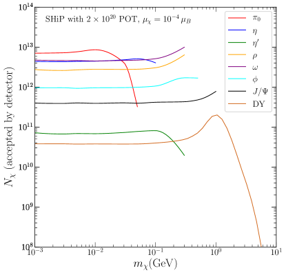
At proton-beam experiments, dark states coupled to the photon can be produced via prompt processes (e.g. DY process or proton bremsstrahlung) and secondary processes (e.g. in meson decays or secondary collisions). In this section, we discuss these production processes and provide the calculations of dominant channels. Numerical results, taking the SHiP experiment as an example, are shown in Fig. 1. The relative importance of the individual contributions does not change significantly from experiment to experiment.
III.1 Drell-Yan Production
Dark states with effective couplings to the photon can be pair-produced directly through quark-antiquark annihilation. To correctly estimate the production from proton-proton collision, we utilize the event generator MadGraph 5 Alwall et al. (2014), to obtain the energy spectrum and angular distribution of dark states per collision, denoted as , as a function of energy and the angle between their momentum and the beam axis, .
We then take the thick target limit, and calculate the total yield of dark states from the DY process via
| (5) |
where the proton on target (POT) number is known for each experiment and is the atomic mass number of the target; , are scaling-indices induced by scattering off a nucleus instead of a proton for the DY cross section, and the total scattering cross section, respectively. DY processes can be treated as incoherent and thus . The value of , for inclusive proton-nucleus scattering, typically of the order , depends on the exact target material, and only mildly affects the final results Alekhin et al. (2016). Here we take for graphite, beryllium, iron, molybdenum, and tungsten, respectively.
III.2 Meson Decay
Another important process is the secondary production of a -pair in the decays of scalar/vector mesons through an off-shell photon. Here we consider the scalar mesons , and , as well as vector mesons , , and .
Typically, if the decays of meson into dark states are kinematically allowed, they tend to dominate the production rate. For example, Harnik et al. (2019) shows that the production of milli-charged particles from meson decay is several orders of magnitude larger than that from DY. Among them, the decay contribution is the most important. However, this picture changes when one considers higher-dimensional operators. This is because the decay rate of light mesons into -pairs will receive additional suppression from their masses, as shown below.
For scalar mesons, the dominant decay channel producing dark states is a three-body decay with final states . By factorizing out the dark current part, we infer that
| (6) |
where the subscript “” denotes “scalar meson”. The branching ratios, , are taken from the PDG Tanabashi et al. (2018). It is worthwhile pointing out that in this step we neglect the mild -dependence induced by the meson transition form factors . Such approximation is particularly justified for the lighter mesons: the photon virtuality is limited by kinematics, and corrections enter at the level of where is the -meson mass; see e.g. Hoferichter et al. (2014); Escribano et al. (2015); Husek (2019a) and Fig. 7 in App. A. To calculate and thus the ratio of the two channels, we follow our previous methodology in Chu et al. (2019a, b) and provide the corresponding expressions in App. A.
A vector meson, in turn, can decay into a pair directly. Thus we compute the branching ratio , where the subscript “” denotes “vector meson”. For two-body decays, one can separate the decay amplitude and phase space factors to obtain
| (7) |
where the last two factors count the differences induced by the interaction type and the phase space, respectively. The expression of for each interaction type is given in App. A, and has previously been derived in Chu et al. (2019a, b). In contrast to the (milli-)charged case (), the function heavily relies on the meson mass for higher-dimensional operators, and the production rate becomes enhanced for heavier meson decay; for more details see the appendix.
To calculate the production rate, the energy and angular distributions of the produced scalar/vector mesons are required. However, the latter are still poorly understood. One reasonable method is to estimate the normalized neutral meson distribution using charged meson distributions. Taking the neutral pion as an example, we follow deNiverville et al. (2017) and stipulate that and write the distribution as
| (8) |
where is the energy of the pion and is its respective emission angle relative to the beam axis. For charged meson distributions, we follow the literature and use the Burman-Smith parameterization Burman and Smith (1989) for sub-GeV kinetic energy proton beams such as LSND, use the Sanford-Wang distribution Aguilar-Arevalo et al. (2009a) for moderate beam energies (several GeV) such as MiniBooNE, and use the so-called BMPT distribution Bonesini et al. (2001) for larger beam energies (from tens of GeV to hundreds of GeV), such as for DUNE and SHiP.
Besides the normalized meson distribution discussed above, we also require the total number of produced mesons in each experiment. For this, we use PYTHIA 8.2 Sjostrand et al. (2006); Sjöstrand et al. (2015) to simulate collisions, and list the average number of mesons produced per POT for each experiment in Tab. 1. We assume that these meson production rates per POT remain the same for collisions; for the latter, current detailed simulations yield differing results, see, e.g., Darmé et al. (2020) for a recent discussion.111Although photo-production of light scalar mesons is known to scale as Krusche (2005) and the scaling-index for inclusive scattering is about as mentioned above, effects of showers and the nuclear medium require dedicated simulations/measurements. The meson multiplicities of our Tab. 1 lie within the range of their adopted values in previous works, e.g. Batell et al. (2014); deNiverville (8 30); CER (2016); deNiverville and Frugiuele (2019); De Romeri et al. (2019); Döbrich et al. (2019); Darmé et al. (2020), and we estimate the uncertainties only affect the final bounds by a factor of at most. Finally, we have also extracted the information on their momentum and angular distributions from PYTHIA 8.2, which is consistent with the fitted distributions mentioned above Döbrich et al. (2019).
For the final distribution function of particles from meson decay in the lab frame we find
| (9) |
where , and are defined in the meson rest frame and denote respectively the energy, as well as the polar and azimuthal angles of the momentum w.r.t. the direction of the boosted meson. In contrast, and are defined in lab frame, and represent the energy of and the angle of the momentum w.r.t. the beam axis. At last, and , the energy of the meson and the angle of the meson momentum w.r.t. the beam axis in lab frame, are functions of , , , and . The dark state spectrum from each meson decay, , is defined as
| (10) |
where the factor accounts for the pair production of dark states and is the aforementioned or , depending on the spin of the meson. Their exact expressions are given in App. A. Note that to obtain Eq. (9) we have used the fact that the meson decay at rest is isotropic.
In practice, we perform Monte Carlo simulations to numerically obtain the distribution function of from meson decay, instead of integrating Eq. (9) directly, as the latter is prohibitively time-consuming.
III.3 Other production mechanisms
Here we discuss additional channels of -pair production. Prominently, proton-nucleus bremsstrahlung contributes to the production of particles. The process can e.g. be estimated using the Fermi-Weizsäcker-Williams method Fermi (1924); von Weizsacker (1934); Williams (1934), as has been done in Blümlein and Brunner (2014); deNiverville et al. (2017); Feng et al. (2018); Tsai et al. (2019). However, for the higher-dimensional interactions studied here, the production of -pairs through bremsstrahlung is generally dominated by the contribution of the vector meson resonance at Faessler et al. (2010). Since we have already taken into account the resonant contribution through the vector meson decay processes above, we will not consider the proton bremsstrahlung any further; thereby we also avoid any double-counting.
Another source of -pair production is the capture of pions onto nuclei or protons via . This process will mostly result in low-energy -particles and is not considered further here. At last, secondary collisions, e.g. between secondary electrons/photons and the target, should not appreciably contribute to the yield in our framework. We always neglect the latter contributions in this work.
IV Detection of dark states
The dark states, produced in proton-nucleus collisions, travel relativistically through the shield into the downstream detector, leading to observable signals. In this work, we focus on their elastic scattering with electrons in the detector (LSND, MiniBooNE-DM, CHARM II, DUNE, SHiP) and hadronic shower signals caused by nuclear deep inelastic scattering (DIS) in E613.
For simplicity, we will approximate the detector-shapes as cylinders with a constant transverse cross-sectional area and a certain depth. Thus, the geometric acceptance of the dark states is determined by the target-detector distance and an effective size. For the nearly spherical detector in MiniBooNE-DM, we take the geometry into account in deriving the signal rate.
IV.1 Scattering on electrons
When entering the detector, particles may scatter with electrons and cause detectable recoil signals. Following Chu et al. (2019a), the master formula to calculate the number of signal events reads
| (11) |
where is the electron number density of the target, is the depth of the detector, is the electron recoil energy with respective experimental threshold and cutoff energies and , is the initial energy in lab frame, and is the detection efficiency. The minimal energy of dark states can be expressed in terms of as
| (12) |
where is target mass, i.e. the electron mass in this case. The differential scattering cross section, , is found in App. E of Chu et al. (2019a).
The spectrum of dark states that have entered the detector, , is obtained by summing up all production processes in the previous section, and applying the detector geometric cut,
| (13) |
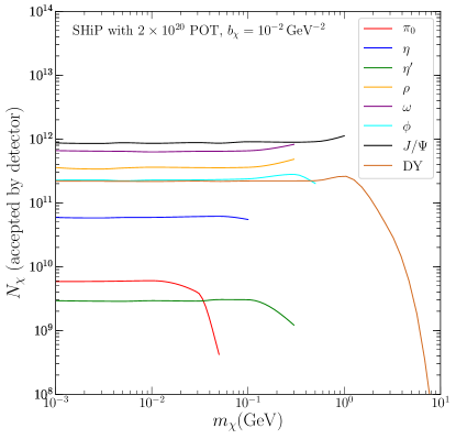
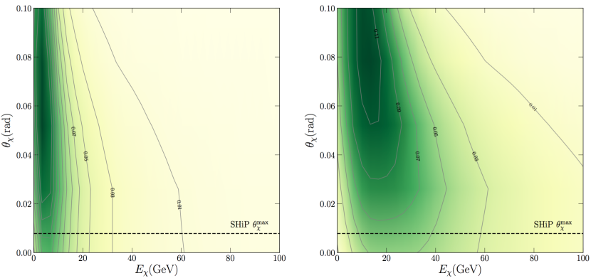
The maximum opening angle is obtained from the target-detector distance and the effective size of the detector. This is illustrated in Fig. 2 for the SHiP experiment (400 GeV proton) and Fig. 3 for the MiniBooNE-DM experiment (8 GeV proton), where only particles below the horizontal dashed line () enter the detector. For the purpose of illustration, the two figures give the contours of , normalized as per particle via
| (14) |
which is obviously independent of the values of form factor couplings.
As shown by the figures, only about – of the total number of particles produced reach the detectors, and this strongly suppresses the number of final events at low energy experiments, such as at MiniBooNE-DM.222This is also one of the motivations for off-axis detectors in proton-beam experiments; see e.g. Coloma et al. (2016); Frugiuele (2017); de Gouvêa et al. (2019). Moreover, such reduction becomes more severe for dark particles generated from heavy meson decay, and is largely insensitive to for particles from DY processes. Besides, for higher-dimensional operators, a preference for more energetic particles can also be observed by comparing the left and right panels in Fig. 2 (also in Fig. 3). This is due to their different energy-dependence in the production rate, and will be further discussed in Sec. VI.1.
Several experiments also make cuts on the electron recoil angle, , in order to reduce backgrounds. From kinematics, the recoil energy can be expressed in terms of and as
| (15) |
where . Hence, we take the cuts on as a further requirement on the boundaries of , where () give upper (lower) limits on .
For the spherical detector in the MiniBooNE-DM experiment, we use an incoming angle-dependent depth for the detector, which reads
| (16) |
where the radius of the detector , and the distance between the collision point and the detector center .
Finally, we note in passing that while we focus on electron recoil signals, which in general provide better bounds, the expressions above are easily generalized to describe nucleon recoils.
IV.2 Hadronic showers
The dark states may also cause hadronic showers, which is relevant for E613. Following Soper et al. (2014) we consider the deep inelastic scattering of with nucleons as the energy deposition process, while neglecting any coherence effects since the typical momentum transfer is larger than the QCD confinement scale. It is worth pointing out that we do not consider the possibility of multiple scatterings in the detector, since the coupling between the particle and the photon is assumed to be weak; see Sec. IV.3.
To derive the expected number of signal events, we first compute the differential cross section of - deep inelastic scattering. The 4-momentum of before (after) scattering is denoted as (). The momentum transfer carried by the intermediate photon is defined as , which is spacelike. Following the DIS formalism for leptons, we introduce the Bjorken variable , with being the nucleon mass, and being the energy transfer in the rest frame of the nucleons. The differential cross section is then written as
| (17) |
where the dark current can be written in terms of the vertex factors of Sec. II,
| (18) |
with the factor coming from average over initial state -spins. The hadronic tensor may be expressed as
| (19) |
in which
| (20) |
with being the 4-momentum of the nucleon before the scattering. We adopt the results for the two structure functions as
| (21) |
where is the charge of quarks in unit of electron charge. We sum over flavors of light quarks/antiquarks, , and use the values of parton distribution function averaged over nucleons for each corresponding nucleus from Hirai et al. (2007).333Such parameterization is numerically equivalent to the one of Soper et al. (2014) in the limit of , which is the case in E613.
The expected number of signal events is given by
| (22) |
where is the number density of nucleons in the detector. The integration boundaries for and are derived from kinematics as
| (23) |
where is the experiment-specific threshold energy. The squared momentum transfer lies in the range
| (24) |
Finally, there is the general requirement .
IV.3 Mean-free-path of dark states
As already mentioned above, our calculations are based on the assumption that particles travel freely, both in the shield and in the detector. This may be validated by estimating the mean free path of , using transport cross section of -proton scatterings,
| (25) |
where is the proton number density. The transport cross section is used as it removes the influence of soft scatterings that would not attenuate the flux of dark particles.
To obtain an estimate, we use the elastic scattering processes for which the formulæ can be found in App. E of Chu et al. (2019a). Here we take the typical distance between the collision point and the detector to be 100 m and the dump/shield mass density to be 10 g/cm3. By requiring m, one can see that these proton-beam experiments are sensitive to the EM form factor parameters
| (26) |
for sub-GeV particles with GeV. As parameters larger than these values above are already excluded by other probes, we may always assume that particles scatter at best once inside the entire experimental setup.
V Experiments
| Experiments | POT () | Signal process and cuts | on/off axis | Reference | |||
|---|---|---|---|---|---|---|---|
| LSND | 1800 | - | e-recoil (, ) | 0.16 | Athanassopoulos et al. (1997); deNiverville (8 30) | ||
| MiniBooNE-DM | 1.86 | e-recoil (, ) | 0 | 0.2 | Aguilar-Arevalo et al. (2018b) | ||
| CHARM II | 0.25 | e-recoil (, ) | 5429 | De Winter et al. (1989); Vilain et al. (1994) | |||
| DUNE (10 yr) | 11/yr | e-recoil (, ) | 8930/yr | 0.5 | Brown (2018); Hostert (2019) | ||
| SHiP | 2 | e-recoil (, ) | 846 | Anelli et al. (2015); Buonocore et al. (2019a) | |||
| E613 | 0.0018 | 12.8 mrad | had. shower ( per event) | Soper et al. (2014); Ball et al. (1980) |
In this section, we briefly review the relevant details of each experiment under consideration. In order to derive the ensuing 90% C.L. limits, we require that the number of events generated by the dark states,
| (27) |
where is the number of actual observed events and is the expected number of background events. When making forecasts for future experiments, we assume . The standard criterion is adopted if no events were observed. For each experiment, the summary of relevant parameters can be found in Table. 2.
V.1 LSND
At the Liquid Scintillator Neutrino Detector (LSND) experiment, a proton beam of kinetic energy was conducted onto water or a high- target such as copper Athanassopoulos et al. (1997). The detector was located at a distance of from the beam dump, with an off-axis angle of , and an active volume comprised of an long cylinder with a diameter of , filled with 167 tonnes of mineral oil Mills (2001).
Due to the low beam energy, we consider decay as the only production channel in LSND as other heavier mesons decay and DY channels are suppressed. As it is difficult to generate the total production rate of in PYTHIA 8.2 at such low energy, we instead estimate it via the ratio , which measurements put at a value of approximately 0.1 Shimizu et al. (1982); Achilli et al. (2011). Under the assumption that this ratio remains unchanged for proton-nuclear scattering, we adopt the value 0.1/POT as our fiducial value in the calculation. This is close to the production rate of positively charged mesons in LSND, about 0.08/POT Allen et al. (1989), as well as the value used in COHERENT experiment, 0.09/POT Akimov et al. (2019).
In the MDM case with , the flux entering the detector is then approximately
| (28) |
yielding the constraint . This can be rescaled to compare with the LSND results Auerbach et al. (2001), which estimates that the flux entering the detector, , is about , leading to a bound on ’s MDM at Auerbach et al. (2001). One can see the equality
| (29) |
is approximately satisfied, suggesting that our treatment of the detector works well.
V.2 MiniBooNE-DM
The Booster Neutrino Experiment, MiniBooNE, operates at the Fermi National Accelerator Aguilar-Arevalo et al. (2009b). The Booster delivers a proton beam with kinetic energy () on a beryllium () target. The center of the spherical on-axis detector is placed downstream from the beam dump with a diameter of filled with 818 tonnes of mineral oil (). In practice, we are more interested in the off-target mode of MiniBooNE, where the proton beam hits directly the steel beam dump, with an ensuing smaller high-energy neutrino background. This is referred to as MiniBooNE-DM, which has data with POT Aguilar-Arevalo et al. (2018b). By only focusing on electrons with extremely small recoil angles, the background was effectively reduced to zero in this off-target mode Aguilar-Arevalo et al. (2018b). That is, we derive the 90% C.L. limits on the couplings of dark states to the photon by requiring .
It is well known that in the on-target mode with POT, MiniBooNE reported a significant excess of electron-like events Aguilar-Arevalo et al. (2018a). In addition, the background event of a single electron recoil is estimated to be about one hundred, after the same cuts as above Dharmapalan et al. (2012). Substituting these values into Eq. (22) in turn suggests that the on-target mode should lead to slightly weaker limits than those from MiniBooNE-DM, despite its larger POT number.
V.3 CHARM II
CERN High energy AcceleRator Mixed field facility II (CHARM II) was a fixed-target experiment designed for a precision measurement of the weak angle. It utilized a 450 GeV proton beam on a Be target, and collected data with POT during 1987-1991 Vilain et al. (1994). The main detector is a 692 t glass calorimeter (SiO2, on average per nucleus), and has an active area of m2, about 870 m away from the target along the beam axis De Winter et al. (1989). In this study, we focus on the single electron recoil signals, as the detector has an almost 100% efficiency to record electromagnetic showers for recoil energy GeV.
To estimate the number of background events, we take reported in Vilain et al. (1994), largely induced by electron scattering with energetic particles. This estimation is conservative, as CHARM II was able to determine the value of the Weinberg angle with the uncertainty below several percents.
V.4 DUNE
The Deep Underground Neutrino Experiment (DUNE) is proposed to be performed at the Long-Baseline Neutrino Facility (LBNF), and can be used to probe light dark particles Acciarri et al. (2015); Abi et al. (2017). At DUNE, a graphite () target is hit by a proton beam with an initial energy . The near detector (75 t fiducial mass) will be placed downstream from the target. It is on-axis and a parallelepiped with a size and we use m as its effective depth Harnik et al. (2019). The detector is filled with liquid Argon (LAr).
We take a 10-year run of the DUNE experiment, with a total POT of . The observable signals we consider for DUNE are single electron events caused by - scatterings. The detection efficiency is assumed to be for the LAr time projection chamber. Following Hostert (2019); De Romeri et al. (2019), we require the cut on the electron recoil angle to satisfy MeV, which significantly reduces the number of background events from charged-current - scattering; see Tab. 2 for details of the parameters.
V.5 SHiP
A fixed-target facility to Search for Hidden Particles (SHiP) is proposed at the CERN super proton synchrotron (SPS) accelerator Anelli et al. (2015). At the SPS facility, a proton beam with () is deployed to collide with the titanium-zirconium doped molybdenum target (). An emulsion cloud chamber detector will be located downstream from the target, and it will be filled with layers of nuclear emulsion films. Following the latest SHiP report collaboration (2019), the size of the detector ( 8 tonnes) is set to be . We assume a 100% detection efficiency for simplicity.444A unity efficiency was also used in Buonocore et al. (2019a); Jodłowski et al. (2019).
The detection process we consider for SHiP is also - scatterings. With POT after 5-years of operation the number of background events is estimated to be , which is dominated by quasi-elastic scattering with a soft final state proton collaboration (2019).
V.6 E613
E613 was a beam dump experiment at Fermilab, set up to study neutrino production, with a proton beam hitting a tungsten target Ball et al. (1980). The detector, away from the target, consisted of 200 tonnes lead plus liquid scintillator. Its size was , with a mass density of about . In order to compare with the previous results Soper et al. (2014); Mohanty and Rao (2015), we only consider a circular region of the detector with a radius of 0.75 m along the beam axis. Moreover, for nucleon-recoil events in E613, the energy deposit needs to be larger than 20 GeV, in order to be recorded. We require the number of such events to be below 180 during its POT run to obtain the constraints.
We assume a thick target so that each incident proton scatters once. This is different from the treatment by Soper et al. (2014); Mohanty and Rao (2015), which estimated the number of scatter events per POT following the scaling
| (30) |
with () being the total length (the nucleon number density) of the target, and the scattering cross section between proton and target. For E613, where is much larger than the mean-free-path of a 400 GeV proton (a few cm in tungsten), Eq. (30) significantly over-estimates the total number of produced particles. As a result, our limits are weaker than those derived in Mohanty and Rao (2015). We revise the previous results in the next section.

V.7 Other experiments
There also exist many other proton-beam experiments which adopt similar setups to those we have studied above, such as COHERENT with a 1 GeV proton beam Akimov et al. (2017), JSNS2 with a 3 GeV proton beam Ajimura et al. (2017), NOA with a 120 GeV proton beam Adamson et al. (2017), as well as WA66 with a 400 GeV proton beam Talebzadeh et al. (1987). Nevertheless, these experiments are in general not expected to provide noticeably stronger (projected) bounds than those obtained above (see e.g. Cooper-Sarkar et al. (1992); Ge and Shoemaker (2018); deNiverville and Frugiuele (2019); Jordan et al. (2018); Buonocore et al. (2019b); Akimov et al. (2019)), and are thus not further studied in this work.
A different new bound on light dark states comes from the NA62 experiment, which has recently improved the constraint on by three orders of magnitude Cortina Gil et al. (2019). This puts upper bounds on the MDM/EDM interactions of our interest as
| (31) |
for . They are weaker than the bounds obtained above, and become even weaker for higher-dimensional operators, i.e. the AM/CR interactions.
High-energy colliders become more important for particles heavier than pions. For instance, at LHC, the upgrade of the MoEDAL experiment will be equipped with three deep liquid scintillator layers Pinfold (2019). In addition, there will be the milliQan detector Haas et al. (2015); Ball et al. (2016) which will be composed of three stacks of plastic scintillators. Both experiments are designed to be sensitive to milli-charged dark particles, of which the scattering cross section with electron/nucleus is dramatically enhanced at low momentum-transfer. As suggested in Sher and Stevens (2018); Frank et al. (2019), such experiments will constrain the EDM form factor of dark states, where there also exists an enhancement—although milder—in low momentum-transfer - (-) region of elastic scattering. Moreover, proposed future colliders, such as HL-LHC and ILC, will be able to further improve the experimental sensitivity on all the EM form factors studied here; see e.g. Kadota and Silk (2014); Primulando et al. (2015); Alves et al. (2018).
VI Results
In this section, we first compare the production efficiency of various production channels, and then summarize our bounds on the EM form factors of dark states.
VI.1 Comparison of Production Channels
In contrast to dark state-photon interactions through milli-charge, higher-dimensional operators are considered in this work. Therefore, dimensional analysis demands an extra energy scale to compensate for the presence of the dimensionful coupling ( for dimension-5 operators and for dimension-6 operators) in cross sections and branching ratios, in comparison to the dimension-4 case. This typically suppresses the yield of dark states.
For DY, the relevant energy scale is of the order of the collision energy, . We can then infer that for dimension-5 (dimension-6) operators the resulting cross section will contain a dimensionless factor and ( and ).555The use of effective operators is justified when these products do not exceed unity. This is not guaranteed in the top portions of Figs. 4 and 5, but we expect that the region remains excluded by associated LEP bounds that resolve the UV particle content. We leave a derivation of such UV-dependent high-energy collider constraints for dedicated future work. Thus, the cross sections involving dimension-5 and 6 operators are further suppressed relative to dimension-4 interactions for and , which incidentally are also required for the treatment of Eqs. (1) and (2) as effective operators. As a result, the DY process gains in relevance relative to the meson decay in the production of particles, especially for dimension-6 operators as for the latter, the relevant energy scale is roughly the meson mass.
In addition, because of the mass-scaling, the relative importance of decaying meson contributions is also modified. The branching ratios into -pairs from light mesons become suppressed. Therefore, we can see that although heavier mesons are produced at lower rates, as shown in Tab. 1, the final yields of dark states from their decay are comparable to (dominate over) those from light mesons for dimension-5 (dimension-6) operators.
The production rate of each channel, after applying the geometric cut, is demonstrated in Fig. 1. One can see that due to the reasons above, the overall pattern in our production rate becomes very different from those of milli-charged particles (see e.g. Harnik et al. (2019)) and dark photons (see e.g. deNiverville et al. (2017)), where light meson decay is the most important production channel unless it is kinematically suppressed.666We have checked that our code reproduces Fig. 2 of Harnik et al. (2019) when switching the effective operators to the milli-charged interaction.
VI.2 Constraints
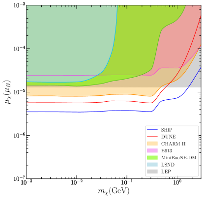
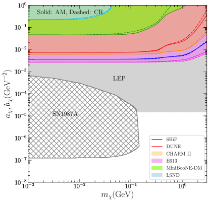
The 90% C.L. constraints on the EM form factors derived above are shown by the colored regions in Fig. 4 (MDM and EDM) and Fig. 5 (AM and CR), together with our previous constraints (gray regions) Chu et al. (2019a, b). As explained above, the strengths of higher-dimensional interactions are energy-sensitive, and constraints derived from current proton-beam experiments, with below several to tens of GeV, turn out not to be competitive with the constraint from LEP Chu et al. (2019a). For dimension-5 operators, future experiments such as DUNE (10-year) and SHiP will improve the sensitivity by a factor of 2–3, and become stronger than LEP for due to their high intensity. It is worth pointing out that the astrophysical bound from SN1987A constrains the MeV-region below Chu et al. (2019b), well below the current and projected experimental sensitivity.
For dimension-6 operators, the production and detection rates of light dark states are even more sensitive to the center-of-mass energy, suggesting it is unlikely for low-energy experiments to play any role in the foreseeable future. In E613 the initial energy of needs to be above 20 GeV to trigger an observable signal, but such large also enhances the -proton scattering, making it difficult for particles to travel through the shield unless GeV-2.777In this region, the validity of the use of effective operators is also in question. Thus, future high energy colliders have better potential to probe dimension-6 dark state interactions.
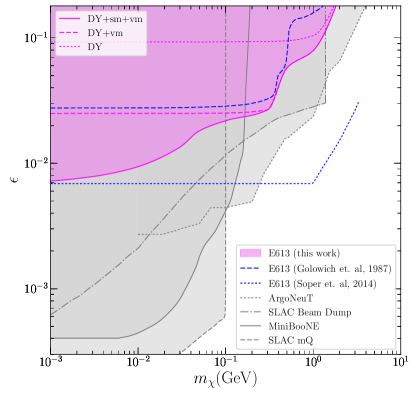
At last, due to the consideration given in Sec. V.6, we also revise the E613 bound on milli-charged particles from Soper et al. (2014), although it has been surpassed by bounds derived from later experiments Prinz et al. (1998); Magill et al. (2019); Liu and Zhang (2019); Gninenko et al. (2019); Chu et al. (2019a). Our derivation also improves w.r.t. a much earlier work Golowich and Robinett (1987), by adding the production through decays of scalar mesons and by imposing the BMPT distribution for mesons. As shown in Fig. 6, if only DY processes are taken into account, our bound is weaker than that from Soper et al. (2014) by about a factor of 7. By adding contributions from vector meson decay, the bound becomes stronger, approximately in agreement with Golowich and Robinett (1987) (dashed lines). Our final exclusion limit, taking into account all these contributions, is shown as the pink shaded region in the figure.
VII Conclusions
In this work we study the production and detection of neutral fermionic dark states that carry EM form factors in proton-beam experiments. We consider the production of -pairs in the collision of high-intensity protons on nuclear targets through prompt Drell-Yan scattering and in secondary meson decays. The detectable signals considered are single electron recoil events at LSND and MiniBooNE-DM, CHARM II, as well as at the proposed DUNE and SHiP experiments, and hadronic showers caused by nuclear deep inelastic scattering at E613.
Owing to the higher dimensionality of the considered operators (dimension 5 and 6), the relative importance of production channels is biased towards processes with larger intrinsic energy. As a consequence, Drell-Yan production and production in heavy meson decays gain prominence when compared to the milli-charged and dark photon cases, for which pion decays dominate the dark state yield.
We compute in detail the energy and angular distribution of the produced dark state flux and set the strongest constraints on the existence of -particles with MDM and EDM interactions in the MeV-GeV mass bracket, excluding dimensionful coefficients , corresponding to an effective scale . For the dimension-6 AM and CR interactions, we find are excluded, pointing towards a comparably lower effective scale of . In the latter case, the constraint is superseded by LEP. Finally, as a by-product of our study, we also revise previously obtained proton-beam dump bounds on milli-charged particles.
With a strong connection to the neutrino program, proton beam experiments constitute an active and diverse field, with a number of new experiments proposed such as SHiP and DUNE. However, because the interactions considered here are higher-dimensional, we find that the prospects of significantly improving the direct sensitivity on EM form factor couplings rather hinges on the future of high-energy collider experiments and their ability to produce collisions with an ever increased center-of-mass energy.
Acknowledgments
We thank Giacomo Marocco, Samuel McDermott, and Subir Sarkar for useful discussions. The authors are supported by the New Frontiers program of the Austrian Academy of Sciences. JLK is supported by the Austrian Science Fund FWF under the Doctoral Program W1252-N27 Particles and Interactions. We acknowledge the use of computer packages for algebraic calculations Mertig et al. (1991); Shtabovenko et al. (2016).
Appendix A Decay rates of scalar mesons
The decay rate of scalar mesons into a photon plus a -pair, , is given by
| (32) |
where is the decay rate with an off-shell photon,
| (33) |
with being the decay constant of the meson. Since we are allowed to neglect the momentum-dependence of the EM transition form factors of the scalar mesons (shown below), will drop out in the branching ratio, Eq. (6).
In Eq. (32), the function is defined by the phase space integral of the squared amplitude of
with . The explicit expressions of were already obtained in Chu et al. (2019a), and are also listed below:
| (34) | |||||
| (35) | |||||
| (36) | |||||
| (37) | |||||
| (38) |
The expression for , used for vector meson decay in Sec. III.2, is then given by
| (39) |
To infer the energy spectrum of from scalar meson decay, we also need to know the differential decay rate in the rest frame of the meson (). To this end, we first compute the amplitude of the process . and define the two Lorentz-invariant variables and , so that becomes . The corresponding squared amplitudes, summed over the spin of final states for each EM form factor are obtained as follows:
| (40) | |||||
| (41) | |||||
| (42) | |||||
| (43) | |||||
| (44) |
Then the Dalitz plot allows us to express the differential decay rate in the rest frame of the meson as
| (45) |
where the integration boundaries of are given by
| (46) |
Here, is
| (47) |
The allowed kinematic range of is . At last we arrive at the differential branching ratio via
| (48) |
from which one can directly see that the meson decay constant, , cancels out in the ratio of and .
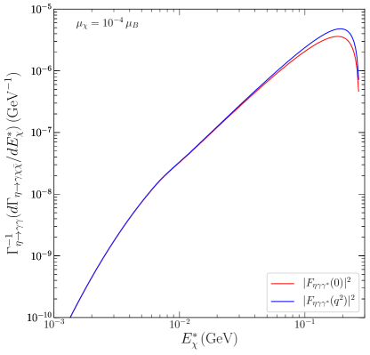
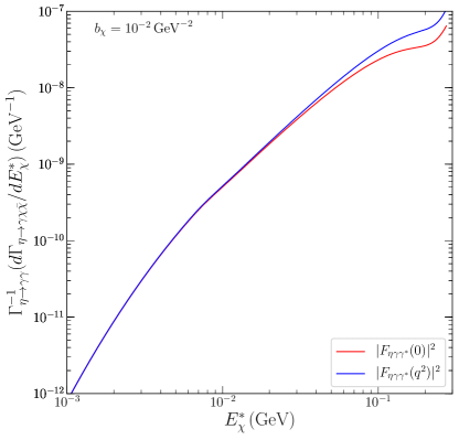
At the end of this section, we comment on the assumption of using constant transition form factors for scalar meson decay. Vector meson dominance suggests that the assumption holds well for , which is the case for decays. For the heavier scalar mesons considered in this work, , we have numerically evaluated the differential decay rate using the EM transition form factor. For the meson Husek (2019b), the results are given in Fig. 7, which shows that the shape of is only affected mildly by the (kinematically limited) virtuality of the intermediate photon. In the total decay rate for MeV, would increase by a factor of 1.3 (1.7) in the case of MDM/EDM, and by a factor of 1.8 (1.9) in the case of AM/CR. Hence, neglecting the momentum-dependence of the transition form factors leads to slightly weaker bounds, and is hence conservative.
Appendix B distribution from meson decay
In this section, the derivation of Eq. (9) is provided. In general, the number of particles produced from a certain meson distribution is given by
| (49) | |||||
where and are the energy of meson and angle between the meson momentum and the beam axis in the lab frame, respectively. The energy of in the rest frame of the meson is denoted by . Finally, , are the polar and azimuthal angles of the momentum in the rest frame of the meson w.r.t. the lab-frame meson momentum.
In practice, we are interested in the distribution of particles in terms of and , which are the energy of and the polar angle of the momentum w.r.t. the beam axis in the lab frame. A Lorentz transformation allows to express the last quantities as functions of , , , and . Then, by inserting the two delta-functions
into Eq. (49) and using the fact that the decay is isotropic in meson rest frame, we arrive at
| (50) | |||||
Next we use the two delta functions to perform the integrals over and leading to,
| (51) |
where the last factor is the Jacobian of the variable transformation.
In the end, the distribution function of particles from meson decay in the lab frame in terms of and reads
| (52) |
Summing up the contribution from each meson, we retrieve Eq. (9) of the main text.
Appendix C in DIS cross section
The DIS differential cross section, given in Eq. (17), contains the contraction of dark and hadronic matrix element . In the following we list for each EM form factor interaction:
| (53) | |||||
| (54) | |||||
| (55) | |||||
| (56) | |||||
| (57) |
References
- Athanassopoulos et al. (1997) C. Athanassopoulos et al. (LSND), Nucl. Instrum. Meth. A388, 149 (1997), arXiv:nucl-ex/9605002 [nucl-ex] .
- Aguilar-Arevalo et al. (2018a) A. A. Aguilar-Arevalo et al. (MiniBooNE), (2018a), arXiv:1805.12028 [hep-ex] .
- Akimov et al. (2017) D. Akimov et al. (COHERENT), Science 357, 1123 (2017), arXiv:1708.01294 [nucl-ex] .
- Acciarri et al. (2015) R. Acciarri et al. (DUNE), (2015), arXiv:1512.06148 [physics.ins-det] .
- Huber et al. (2004) P. Huber, M. Lindner, M. Rolinec, T. Schwetz, and W. Winter, Phys. Rev. D70, 073014 (2004), arXiv:hep-ph/0403068 [hep-ph] .
- Alexander et al. (2016) J. Alexander et al. (2016) arXiv:1608.08632 [hep-ph] .
- Essig et al. (2013) R. Essig et al., in Proceedings, 2013 Community Summer Study on the Future of U.S. Particle Physics: Snowmass on the Mississippi (CSS2013): Minneapolis, MN, USA, July 29-August 6, 2013 (2013) arXiv:1311.0029 [hep-ph] .
- Golowich and Robinett (1987) E. Golowich and R. W. Robinett, Phys. Rev. D35, 391 (1987).
- Prinz et al. (1998) A. A. Prinz et al., Phys. Rev. Lett. 81, 1175 (1998), arXiv:hep-ex/9804008 [hep-ex] .
- Izaguirre et al. (2013) E. Izaguirre, G. Krnjaic, P. Schuster, and N. Toro, Phys. Rev. D88, 114015 (2013), arXiv:1307.6554 [hep-ph] .
- Soper et al. (2014) D. E. Soper, M. Spannowsky, C. J. Wallace, and T. M. P. Tait, Phys. Rev. D90, 115005 (2014), arXiv:1407.2623 [hep-ph] .
- Berlin et al. (2019) A. Berlin, N. Blinov, G. Krnjaic, P. Schuster, and N. Toro, Phys. Rev. D99, 075001 (2019), arXiv:1807.01730 [hep-ph] .
- Magill et al. (2019) G. Magill, R. Plestid, M. Pospelov, and Y.-D. Tsai, Phys. Rev. Lett. 122, 071801 (2019), arXiv:1806.03310 [hep-ph] .
- Liang et al. (2019) J. Liang, Z. Liu, Y. Ma, and Y. Zhang, (2019), arXiv:1909.06847 [hep-ph] .
- Davidson et al. (2000) S. Davidson, S. Hannestad, and G. Raffelt, JHEP 05, 003 (2000), arXiv:hep-ph/0001179 [hep-ph] .
- Dubovsky et al. (2004) S. L. Dubovsky, D. S. Gorbunov, and G. I. Rubtsov, JETP Lett. 79, 1 (2004), [Pisma Zh. Eksp. Teor. Fiz.79,3(2004)], arXiv:hep-ph/0311189 [hep-ph] .
- McDermott et al. (2011) S. D. McDermott, H.-B. Yu, and K. M. Zurek, Phys. Rev. D83, 063509 (2011), arXiv:1011.2907 [hep-ph] .
- Cline et al. (2012) J. M. Cline, Z. Liu, and W. Xue, Phys. Rev. D85, 101302 (2012), arXiv:1201.4858 [hep-ph] .
- Dolgov et al. (2013) A. D. Dolgov, S. L. Dubovsky, G. I. Rubtsov, and I. I. Tkachev, Phys. Rev. D88, 117701 (2013), arXiv:1310.2376 [hep-ph] .
- Vogel and Redondo (2014) H. Vogel and J. Redondo, JCAP 1402, 029 (2014), arXiv:1311.2600 [hep-ph] .
- Dvorkin et al. (2014) C. Dvorkin, K. Blum, and M. Kamionkowski, Phys. Rev. D89, 023519 (2014), arXiv:1311.2937 [astro-ph.CO] .
- Ali-Haïmoud et al. (2015) Y. Ali-Haïmoud, J. Chluba, and M. Kamionkowski, Phys. Rev. Lett. 115, 071304 (2015), arXiv:1506.04745 [astro-ph.CO] .
- Kamada et al. (2017) A. Kamada, K. Kohri, T. Takahashi, and N. Yoshida, Phys. Rev. D95, 023502 (2017), arXiv:1604.07926 [astro-ph.CO] .
- Agrawal and Randall (2017) P. Agrawal and L. Randall, JCAP 1712, 019 (2017), arXiv:1706.04195 [hep-ph] .
- Muñoz and Loeb (2018) J. B. Muñoz and A. Loeb, Nature 557, 684 (2018), arXiv:1802.10094 [astro-ph.CO] .
- Berlin et al. (2018) A. Berlin, D. Hooper, G. Krnjaic, and S. D. McDermott, Phys. Rev. Lett. 121, 011102 (2018), arXiv:1803.02804 [hep-ph] .
- Barkana et al. (2018) R. Barkana, N. J. Outmezguine, D. Redigolo, and T. Volansky, Phys. Rev. D98, 103005 (2018), arXiv:1803.03091 [hep-ph] .
- Chang et al. (2018) J. H. Chang, R. Essig, and S. D. McDermott, JHEP 09, 051 (2018), arXiv:1803.00993 [hep-ph] .
- Kovetz et al. (2018) E. D. Kovetz, V. Poulin, V. Gluscevic, K. K. Boddy, R. Barkana, and M. Kamionkowski, Phys. Rev. D98, 103529 (2018), arXiv:1807.11482 [astro-ph.CO] .
- Xu et al. (2018) W. L. Xu, C. Dvorkin, and A. Chael, Phys. Rev. D97, 103530 (2018), arXiv:1802.06788 [astro-ph.CO] .
- Slatyer and Wu (2018) T. R. Slatyer and C.-L. Wu, Phys. Rev. D98, 023013 (2018), arXiv:1803.09734 [astro-ph.CO] .
- Pospelov and ter Veldhuis (2000) M. Pospelov and T. ter Veldhuis, Phys. Lett. B480, 181 (2000), arXiv:hep-ph/0003010 [hep-ph] .
- Sigurdson et al. (2004) K. Sigurdson, M. Doran, A. Kurylov, R. R. Caldwell, and M. Kamionkowski, Phys. Rev. D70, 083501 (2004), [Erratum: Phys. Rev.D73,089903(2006)], arXiv:astro-ph/0406355 [astro-ph] .
- Ho and Scherrer (2013) C. M. Ho and R. J. Scherrer, Phys. Lett. B722, 341 (2013), arXiv:1211.0503 [hep-ph] .
- Schmidt et al. (2012) D. Schmidt, T. Schwetz, and T. Toma, Phys. Rev. D85, 073009 (2012), arXiv:1201.0906 [hep-ph] .
- Kopp et al. (2014) J. Kopp, L. Michaels, and J. Smirnov, JCAP 1404, 022 (2014), arXiv:1401.6457 [hep-ph] .
- Ibarra and Wild (2015) A. Ibarra and S. Wild, JCAP 1505, 047 (2015), arXiv:1503.03382 [hep-ph] .
- Sandick et al. (2016) P. Sandick, K. Sinha, and F. Teng, JHEP 10, 018 (2016), arXiv:1608.00642 [hep-ph] .
- Kavanagh et al. (2019) B. J. Kavanagh, P. Panci, and R. Ziegler, JHEP 04, 089 (2019), arXiv:1810.00033 [hep-ph] .
- Trickle et al. (2019) T. Trickle, Z. Zhang, and K. M. Zurek, (2019), arXiv:1905.13744 [hep-ph] .
- Chu et al. (2019a) X. Chu, J. Pradler, and L. Semmelrock, Phys. Rev. D99, 015040 (2019a), arXiv:1811.04095 [hep-ph] .
- Banerjee et al. (2017) D. Banerjee et al. (NA64), (2017), arXiv:1710.00971 [hep-ex] .
- Åkesson et al. (2018) T. Åkesson et al. (LDMX), (2018), arXiv:1808.05219 [hep-ex] .
- Battaglieri et al. (2016) M. Battaglieri et al. (BDX), (2016), arXiv:1607.01390 [hep-ex] .
- Aubert et al. (2002) B. Aubert et al. (BaBar), Nucl. Instrum. Meth. A479, 1 (2002), arXiv:hep-ex/0105044 [hep-ex] .
- Abe et al. (2010) T. Abe et al. (Belle-II), (2010), arXiv:1011.0352 [physics.ins-det] .
- Evans and Bryant (2008) L. Evans and P. Bryant, JINST 3, S08001 (2008).
- Aubert et al. (2003) B. Aubert et al. (BaBar), in 38th Rencontres de Moriond on Electroweak Interactions and Unified Theories Les Arcs, France, March 15-22, 2003 (2003) arXiv:hep-ex/0304020 [hep-ex] .
- Bird et al. (2004) C. Bird, P. Jackson, R. V. Kowalewski, and M. Pospelov, Phys. Rev. Lett. 93, 201803 (2004), arXiv:hep-ph/0401195 [hep-ph] .
- Anisimovsky et al. (2004) V. V. Anisimovsky et al. (E949), Phys. Rev. Lett. 93, 031801 (2004), arXiv:hep-ex/0403036 [hep-ex] .
- Artamonov et al. (2009) A. V. Artamonov et al. (BNL-E949), Phys. Rev. D79, 092004 (2009), arXiv:0903.0030 [hep-ex] .
- Tanabashi et al. (2018) M. Tanabashi et al. (Particle Data Group), Phys. Rev. D98, 030001 (2018).
- Jegerlehner and Nyffeler (2009) F. Jegerlehner and A. Nyffeler, Phys. Rept. 477, 1 (2009), arXiv:0902.3360 [hep-ph] .
- Bennett et al. (2006) G. W. Bennett et al. (Muon g-2), Phys. Rev. D73, 072003 (2006), arXiv:hep-ex/0602035 [hep-ex] .
- Saito (2012) N. Saito (J-PARC g-’2/EDM), Proceedings, International Workshop on Grand Unified Theories (GUT2012): Kyoto, Japan, March 15-17, 2012, AIP Conf. Proc. 1467, 45 (2012).
- Grange et al. (2015) J. Grange et al. (Muon g-2), (2015), arXiv:1501.06858 [physics.ins-det] .
- Sirlin (1980) A. Sirlin, Phys. Rev. D22, 971 (1980).
- Chu et al. (2019b) X. Chu, J.-L. Kuo, J. Pradler, and L. Semmelrock, Phys. Rev. D100, 083002 (2019b), arXiv:1908.00553 [hep-ph] .
- Chang et al. (2019) J. H. Chang, R. Essig, and A. Reinert, (2019), arXiv:1911.03389 [hep-ph] .
- Aguilar-Arevalo et al. (2018b) A. A. Aguilar-Arevalo et al. (MiniBooNE DM), Phys. Rev. D98, 112004 (2018b), arXiv:1807.06137 [hep-ex] .
- De Winter et al. (1989) K. De Winter et al. (CHARM-II), Nucl. Instrum. Meth. A278, 670 (1989).
- Vilain et al. (1994) P. Vilain et al. (CHARM-II), Phys. Lett. B335, 246 (1994).
- Ball et al. (1980) R. Ball et al., Proceedings: Mini-Conference and Workshop on Neutrino Mass, Telemark, Wisconsin, Oct 2-4, 1980, eConf C801002, 172 (1980).
- Anelli et al. (2015) M. Anelli et al. (SHiP), (2015), arXiv:1504.04956 [physics.ins-det] .
- Abi et al. (2017) B. Abi et al. (DUNE), (2017), arXiv:1706.07081 [physics.ins-det] .
- Bagnasco et al. (1994) J. Bagnasco, M. Dine, and S. D. Thomas, Phys. Lett. B320, 99 (1994), arXiv:hep-ph/9310290 [hep-ph] .
- Foadi et al. (2009) R. Foadi, M. T. Frandsen, and F. Sannino, Phys. Rev. D80, 037702 (2009), arXiv:0812.3406 [hep-ph] .
- Antipin et al. (2015) O. Antipin, M. Redi, A. Strumia, and E. Vigiani, JHEP 07, 039 (2015), arXiv:1503.08749 [hep-ph] .
- Alwall et al. (2014) J. Alwall, R. Frederix, S. Frixione, V. Hirschi, F. Maltoni, O. Mattelaer, H. S. Shao, T. Stelzer, P. Torrielli, and M. Zaro, JHEP 07, 079 (2014), arXiv:1405.0301 [hep-ph] .
- Alekhin et al. (2016) S. Alekhin et al., Rept. Prog. Phys. 79, 124201 (2016), arXiv:1504.04855 [hep-ph] .
- Harnik et al. (2019) R. Harnik, Z. Liu, and O. Palamara, JHEP 07, 170 (2019), arXiv:1902.03246 [hep-ph] .
- Hoferichter et al. (2014) M. Hoferichter, B. Kubis, S. Leupold, F. Niecknig, and S. P. Schneider, Eur. Phys. J. C74, 3180 (2014), arXiv:1410.4691 [hep-ph] .
- Escribano et al. (2015) R. Escribano, P. Masjuan, and P. Sanchez-Puertas, Eur. Phys. J. C75, 414 (2015), arXiv:1504.07742 [hep-ph] .
- Husek (2019a) T. Husek, Proceedings, 15th International Workshop on Meson Physics (MESON 2018): Kraków, Poland, June 7-12, 2018, EPJ Web Conf. 199, 02015 (2019a), arXiv:1811.12350 [hep-ph] .
- deNiverville et al. (2017) P. deNiverville, C.-Y. Chen, M. Pospelov, and A. Ritz, Phys. Rev. D95, 035006 (2017), arXiv:1609.01770 [hep-ph] .
- Burman and Smith (1989) R. L. Burman and E. S. Smith, (1989).
- Aguilar-Arevalo et al. (2009a) A. A. Aguilar-Arevalo et al. (MiniBooNE), Phys. Rev. D79, 072002 (2009a), arXiv:0806.1449 [hep-ex] .
- Bonesini et al. (2001) M. Bonesini, A. Marchionni, F. Pietropaolo, and T. Tabarelli de Fatis, Eur. Phys. J. C20, 13 (2001), arXiv:hep-ph/0101163 [hep-ph] .
- Sjostrand et al. (2006) T. Sjostrand, S. Mrenna, and P. Z. Skands, JHEP 05, 026 (2006), arXiv:hep-ph/0603175 [hep-ph] .
- Sjöstrand et al. (2015) T. Sjöstrand, S. Ask, J. R. Christiansen, R. Corke, N. Desai, P. Ilten, S. Mrenna, S. Prestel, C. O. Rasmussen, and P. Z. Skands, Comput. Phys. Commun. 191, 159 (2015), arXiv:1410.3012 [hep-ph] .
- Darmé et al. (2020) L. Darmé, S. A. R. Ellis, and T. You, (2020), arXiv:2001.01490 [hep-ph] .
- Krusche (2005) B. Krusche, Lepton scattering and the structure of hadrons and nuclei. Proceedings, International School of nuclear physics, 26th Course, Erice, Italy, September 16-24, 2004, Prog. Part. Nucl. Phys. 55, 46 (2005), arXiv:nucl-ex/0411033 [nucl-ex] .
- Batell et al. (2014) B. Batell, P. deNiverville, D. McKeen, M. Pospelov, and A. Ritz, Phys. Rev. D90, 115014 (2014), arXiv:1405.7049 [hep-ph] .
- deNiverville (8 30) P. deNiverville, Searching for hidden sector dark matter with fixed target neutrino experiments, Ph.D. thesis, U. Victoria (main) (2016-08-30).
- CER (2016) SHiP Collaboration (2016), CERN-SHiP-NOTE-2016-004 .
- deNiverville and Frugiuele (2019) P. deNiverville and C. Frugiuele, Phys. Rev. D99, 051701 (2019), arXiv:1807.06501 [hep-ph] .
- De Romeri et al. (2019) V. De Romeri, K. J. Kelly, and P. A. N. Machado, Phys. Rev. D100, 095010 (2019), arXiv:1903.10505 [hep-ph] .
- Döbrich et al. (2019) B. Döbrich, J. Jaeckel, and T. Spadaro, JHEP 05, 213 (2019), arXiv:1904.02091 [hep-ph] .
- Fermi (1924) E. Fermi, Z. Phys. 29, 315 (1924).
- von Weizsacker (1934) C. F. von Weizsacker, Z. Phys. 88, 612 (1934).
- Williams (1934) E. J. Williams, Phys. Rev. 45 (1934).
- Blümlein and Brunner (2014) J. Blümlein and J. Brunner, Phys. Lett. B731, 320 (2014), arXiv:1311.3870 [hep-ph] .
- Feng et al. (2018) J. L. Feng, I. Galon, F. Kling, and S. Trojanowski, Phys. Rev. D97, 035001 (2018), arXiv:1708.09389 [hep-ph] .
- Tsai et al. (2019) Y.-D. Tsai, P. deNiverville, and M. X. Liu, (2019), arXiv:1908.07525 [hep-ph] .
- Faessler et al. (2010) A. Faessler, M. I. Krivoruchenko, and B. V. Martemyanov, Phys. Rev. C82, 038201 (2010), arXiv:0910.5589 [hep-ph] .
- Coloma et al. (2016) P. Coloma, B. A. Dobrescu, C. Frugiuele, and R. Harnik, JHEP 04, 047 (2016), arXiv:1512.03852 [hep-ph] .
- Frugiuele (2017) C. Frugiuele, Phys. Rev. D96, 015029 (2017), arXiv:1701.05464 [hep-ph] .
- de Gouvêa et al. (2019) A. de Gouvêa, P. J. Fox, R. Harnik, K. J. Kelly, and Y. Zhang, JHEP 01, 001 (2019), arXiv:1809.06388 [hep-ph] .
- Hirai et al. (2007) M. Hirai, S. Kumano, and T. H. Nagai, Phys. Rev. C76, 065207 (2007), arXiv:0709.3038 [hep-ph] .
- Brown (2018) G. R. Brown, Sensitivity Study for Low Mass Dark Matter Search at DUNE, Master’s thesis, Texas U., Arlington (2018).
- Hostert (2019) M. Hostert, Hidden Physics at the Neutrino Frontier: Tridents, Dark Forces, and Hidden Particles, Ph.D. thesis, Durham U. (2019).
- Buonocore et al. (2019a) L. Buonocore, C. Frugiuele, F. Maltoni, O. Mattelaer, and F. Tramontano, JHEP 05, 028 (2019a), arXiv:1812.06771 [hep-ph] .
- Mills (2001) G. B. Mills (LSND), in Proceedings, 34th Rencontres de Moriond on Electroweak Interactions and Unified Theories: Les Arcs, France, Mar 13-20, 1999, The Gioi (The Gioi, Hanoi, 2001) pp. 41–52.
- Shimizu et al. (1982) F. Shimizu, Y. Kubota, H. Koiso, F. Sai, S. Sakamoto, and S. S. Yamamoto, Nucl. Phys. A386, 571 (1982).
- Achilli et al. (2011) A. Achilli, R. M. Godbole, A. Grau, G. Pancheri, O. Shekhovtsova, and Y. N. Srivastava, Phys. Rev. D84, 094009 (2011), arXiv:1102.1949 [hep-ph] .
- Allen et al. (1989) R. C. Allen, H. H. Chen, M. E. Potter, R. L. Burman, J. B. Donahue, D. A. Krakauer, R. L. Talaga, E. S. Smith, and A. C. Dodd, Nucl. Instrum. Meth. A284, 347 (1989).
- Akimov et al. (2019) D. Akimov et al. (COHERENT), (2019), arXiv:1911.06422 [hep-ex] .
- Auerbach et al. (2001) L. B. Auerbach et al. (LSND), Phys. Rev. D63, 112001 (2001), arXiv:hep-ex/0101039 [hep-ex] .
- Aguilar-Arevalo et al. (2009b) A. A. Aguilar-Arevalo et al. (MiniBooNE), Nucl. Instrum. Meth. A599, 28 (2009b), arXiv:0806.4201 [hep-ex] .
- Dharmapalan et al. (2012) R. Dharmapalan et al. (MiniBooNE), (2012), arXiv:1211.2258 [hep-ex] .
- collaboration (2019) S. collaboration (SHiP Collaboration), SHiP Experiment - Comprehensive Design Study report, Tech. Rep. CERN-SPSC-2019-049. SPSC-SR-263 (CERN, Geneva, 2019).
- Jodłowski et al. (2019) K. Jodłowski, F. Kling, L. Roszkowski, and S. Trojanowski, (2019), arXiv:1911.11346 [hep-ph] .
- Mohanty and Rao (2015) S. Mohanty and S. Rao, (2015), arXiv:1506.06462 [hep-ph] .
- Ajimura et al. (2017) S. Ajimura et al., (2017), arXiv:1705.08629 [physics.ins-det] .
- Adamson et al. (2017) P. Adamson et al. (NOvA), Phys. Rev. Lett. 118, 151802 (2017), arXiv:1701.05891 [hep-ex] .
- Talebzadeh et al. (1987) M. Talebzadeh et al. (BEBC WA66), Nucl. Phys. B291, 503 (1987).
- Cooper-Sarkar et al. (1992) A. M. Cooper-Sarkar, S. Sarkar, J. Guy, W. Venus, P. O. Hulth, and K. Hultqvist, Phys. Lett. B280, 153 (1992).
- Ge and Shoemaker (2018) S.-F. Ge and I. M. Shoemaker, JHEP 11, 066 (2018), arXiv:1710.10889 [hep-ph] .
- Jordan et al. (2018) J. R. Jordan, Y. Kahn, G. Krnjaic, M. Moschella, and J. Spitz, Phys. Rev. D98, 075020 (2018), arXiv:1806.05185 [hep-ph] .
- Buonocore et al. (2019b) L. Buonocore, P. deNiverville, and C. Frugiuele, (2019b), arXiv:1912.09346 [hep-ph] .
- Cortina Gil et al. (2019) E. Cortina Gil et al. (NA62), JHEP 05, 182 (2019), arXiv:1903.08767 [hep-ex] .
- Pinfold (2019) J. L. Pinfold, Proceedings, 7th International Conference on New Frontiers in Physics (ICNFP 2018): Kolymbari, Crete, Greece, July 4-12, 2018, Universe 5, 47 (2019).
- Haas et al. (2015) A. Haas, C. S. Hill, E. Izaguirre, and I. Yavin, Phys. Lett. B746, 117 (2015), arXiv:1410.6816 [hep-ph] .
- Ball et al. (2016) A. Ball et al., (2016), arXiv:1607.04669 [physics.ins-det] .
- Sher and Stevens (2018) M. Sher and J. Stevens, Phys. Lett. B777, 246 (2018), arXiv:1710.06894 [hep-ph] .
- Frank et al. (2019) M. Frank, M. de Montigny, P.-P. A. Ouimet, J. Pinfold, A. Shaa, and M. Staelens, (2019), arXiv:1909.05216 [hep-ph] .
- Kadota and Silk (2014) K. Kadota and J. Silk, Phys. Rev. D89, 103528 (2014), arXiv:1402.7295 [hep-ph] .
- Primulando et al. (2015) R. Primulando, E. Salvioni, and Y. Tsai, JHEP 07, 031 (2015), arXiv:1503.04204 [hep-ph] .
- Alves et al. (2018) A. Alves, A. C. O. Santos, and K. Sinha, Phys. Rev. D97, 055023 (2018), arXiv:1710.11290 [hep-ph] .
- Liu and Zhang (2019) Z. Liu and Y. Zhang, Phys. Rev. D99, 015004 (2019), arXiv:1808.00983 [hep-ph] .
- Gninenko et al. (2019) S. N. Gninenko, D. V. Kirpichnikov, and N. V. Krasnikov, Phys. Rev. D100, 035003 (2019), arXiv:1810.06856 [hep-ph] .
- Acciarri et al. (2019) R. Acciarri et al. (ArgoNeuT), (2019), arXiv:1911.07996 [hep-ex] .
- Mertig et al. (1991) R. Mertig, M. Bohm, and A. Denner, Comput. Phys. Commun. 64, 345 (1991).
- Shtabovenko et al. (2016) V. Shtabovenko, R. Mertig, and F. Orellana, Comput. Phys. Commun. 207, 432 (2016), arXiv:1601.01167 [hep-ph] .
- Husek (2019b) T. Husek, in 22nd High-Energy Physics International Conference in Quantum Chromodynamics (QCD 19) Montpellier, Languedoc, France, July 2-5, 2019 (2019) arXiv:1911.06820 [hep-ph] .