Compactly Supported Quasi-tight Multiframelets with High Balancing Orders and Compact Framelet Transforms
Abstract.
Framelets (a.k.a. wavelet frames) are of interest in both theory and applications. Quite often, tight or dual framelets with high vanishing moments are constructed through the popular oblique extension principle (OEP). Though OEP can increase vanishing moments for improved sparsity, it has a serious shortcoming for scalar framelets: the associated discrete framelet transform is often not compact and deconvolution is unavoidable. Here we say that a framelet transform is compact if it can be implemented by convolution using only finitely supported filters. On one hand, [16, Theorem 1.3] proves that for any scalar dual framelet constructed through OEP from any pair of scalar spline refinable functions, if it has a compact discrete framelet transform, then it can have at most one vanishing moment. On the other hand, in sharp contrast to the extensively studied scalar framelets, multiframelets (a.k.a. vector framelets) derived through OEP from refinable vector functions are much less studied and are far from well understood. Also, most constructed multiframelets often lack balancing property which reduces sparsity. In this paper, we are particularly interested in quasi-tight multiframelets, which are special dual multiframelets but behave almost identically as tight multiframelets. From any compactly supported refinable vector function having at least two entries, we prove that we can always construct through OEP a compactly supported quasi-tight multiframelet such that (1) its associated discrete framelet transform is compact and has the highest possible balancing order; (2) all compactly supported framelet generators have the highest possible order of vanishing moments, matching the approximation/accuracy order of its underlying refinable vector function. This result demonstrates great advantages of OEP for multiframelets (retaining all the desired properties) over scalar framelets. The key ingredient of our proof relies on a newly developed normal form of matrix-valued filters, which is of independent interest and importance for greatly reducing the difficulty of studying refinable vector functions and multiframelets/multiwavelets. We also study discrete multiframelet transforms employing OEP-based multiframelet filter banks. To illustrate our theoretical results, we provide a few examples of quasi-tight multiframelets with a compact discrete framelet transform and having the highest possible balancing orders and vanishing moments.
Key words and phrases:
quasi-tight framelets, multiframelets, oblique extension principle, multiwavelets, normal form of a matrix-valued filter, vanishing moments, balancing order, compact framelet transform2010 Mathematics Subject Classification:
42C40, 42C15, 41A25, 41A35, 65T601. Introduction and Main Results
1.1. Backgrounds on Framelets
Wavelets and framelets are of interest in applications such as image processing and numerical algorithms (see e.g. [3, 5, 6, 8, 11, 21] and references therein). Framelets generalize wavelets by allowing redundancy with flexibility. Let us first recall some necessary notations and definitions. In this paper, we mainly deal with vector functions with entries in . By we mean that is an matrix of functions in , and we define
Note that is an matrix of complex numbers. In particular, we define , the space of all column vector of functions in . For , we shall adopt the following notation:
Let be a positive integer with . For vector functions and , we say that is a -framelet in if there exist positive constants and such that
| (1.1) |
where . If (i.e., is a function), then is called a scalar -framelet. If (i.e., is a vector function), then is often called a -multiframelet. For simplicity, in this paper we refer both of them as a framelet. We now recall the definition of a dual -framelet. Let and . We say that is a dual -framelet in if both and are -framelets in , and for all ,
| (1.2) |
with the series converging absolutely. It is straightforward to see that is a dual -framelet if and only if is a dual -framelet in . is called a tight -framelet in if is a dual -framelet. Framelets are often constructed from refinable vector functions. By we denote the set of all finitely supported sequences on . For , we define
which is an matrix of -periodic trigonometric polynomials. A vector function is a -refinable vector function with a (matrix-valued) refinement filter/mask if
Here, the Fourier transform of is defined to be for , and the definition is naturally extended to functions and tempered distributions. is the vector function obtained by taking entry-wise Fourier transform on . If , then is called a (scalar) refinable function. One of the most important examples of refinable scalar functions are B-splines. For , the B-spline function of order is defined by
| (1.3) |
The B-spline function is a piecewise polynomial function, belongs to with support , and is -refinable: with
| (1.4) |
The most general way of deriving framelets from refinable (vector) functions is through the oblique extension principle (OEP), which was introduced in [8] and [3] for scalar framelets. Here let us recall a special version of the oblique extension principle stated in [21, Theorem 6.4.1] (c.f. [16, Theorem 1.1]) for constructing dual framelets from refinable vector functions.
Theorem 1.1.
Let be a positive integer with . Let and be compactly supported -refinable vector functions satisfying and . For finitely supported matrix-valued filters , define
Then is a dual -framelet in if
-
(1)
with ;
-
(2)
all entries in and have at least one vanishing moment, i.e., .
-
(3)
forms an OEP-based dual -framelet filter bank satisfying
(1.5) for all and .
Under the additional assumption that for infinitely many , [21, Theorem 6.4.1] also shows that the above items (1)–(3) are necessary conditions for to be a dual -framelet in . For two smooth functions and , for convenience we shall adopt the following notation: For and ,
The sparsity of the framelet representation in (1.2) is largely due to the vanishing moments of the framelet generators and . A compactly supported vector function has vanishing moments if as . We further define with being the largest such integer. The vanishing moments of in Theorem 1.1 is closely related to the approximation property of the refinable vector function and sum rules of its associated refinement filter/mask . For a finitely supported matrix-valued filter , we say that has sum rules with respect to the dilation factor with a matching filter if and
| (1.6) |
In particular, we define with being the largest possible integer in (1.6). In the scalar case (i.e., ), (1.6) is equivalent to by taking as and noting with .
For a dual -framelet constructed in Theorem 1.1, regardless of the choice of filters and , it is well known through a simple argument that and . From a pair of B-spline filters and in (1.4), any dual -framelet, derived through Theorem 1.1 with the trivial choice , has at most one vanishing moment, i.e., (see [8, 30]), even though can be arbitrarily large. As well explained in [3, 8] (also see [7, 16, 22]), the main advantage of OEP is to increase the orders of vanishing moments of and in Theorem 1.1 by properly choosing the filters and so that and . A lot of compactly supported scalar tight or dual framelets with the highest possible vanishing moments have been constructed in the literature, to mention only a few, see [1, 2, 3, 7, 8, 9, 10, 14, 16, 21, 22, 23, 24, 25, 27, 30, 32] and many references therein. In particular, see Chapter 3 of [21] for comprehensive study and references on scalar tight or dual framelets.
Multiwavelets have certain advantages over scalar wavelets and have been initially studied in [12, 13] and references therein. In sharp contrast to the extensively studied OEP-based scalar framelets, constructing multiframelets (a.k.a. vector framelets) through OEP in Theorem 1.1 is much more difficult than scalar framelets. To our best knowledge, we are only aware of [27, Chapter 2] for studying OEP-based tight multiframelets, and [16, 22] for investigating OEP-based dual multiframelets with vanishing moments. However, as observed in [16], OEP-based dual framelets with OEP-based dual framelet filter banks in Theorem 1.1 has a drawback: their associated discrete framelet transforms are not compact. Here we say that a discrete framelet transform is compact if it can be implemented by convolution using only finitely supported filters. Discrete framelet transforms have been mentioned in [8] for scalar framelets and in [16] for multiframelets. For multiframelets with high vanishing moments and with multiplicity , it is well known that they often have a much lower balancing order (e.g., see [4, 16, 17, 26, 29, 31]), leading to a significant loss of sparsity of their associated discrete multiframelet transform. Since we are not aware of any detailed study on discrete multiframelet transforms using OEP-based filter banks in the literature, we shall study in Section 3 discrete multiframelet transforms using OEP-based matrix-valued filter banks as well as their discrete vanishing moments and balancing property. Then we shall explain in detail in Section 3 why almost all constructed OEP-based dual framelets with OEP-based filter banks in the literature have non-compact discrete multiframelet transforms and cannot avoid nonstable deconvolutions. Such drawbacks of OEP-based scalar framelets and multiframelets make them much less attractive in applications.
1.2. Our Contributions
To avoid all the above-mentioned shortcomings of OEP for multiframelets (see Section 3 for details), in this paper we are particularly interested in quasi-tight multiframelets, which are special dual multiframelets, but behave almost identically as tight multiframelets. Let and . For , we say that is a quasi-tight -framelet in if is a dual -framelet in . Or equivalently, we say that is a quasi-tight -framelet if is a -framelet satisfying (1.1) and
| (1.7) |
with the above series converging unconditionally in , where . Obviously, if , then a quasi-tight -framelet is simply a tight -framelet. One example of quasi-tight framelets appeared in [21, Example 3.2.2]. Scalar quasi-tight framelets have been studied in [10] for dimension one and in [9] for high dimensions with the added feature of directionality. Furthermore, if with is a quasi-tight -framelet in , by [18, Proposition 5], then is a homogeneous quasi-tight -framelet in satisfying (1.1) and
with the above series converging unconditionally in .
We are now ready to state the main result of this paper on quasi-tight multiframelets having all the desired properties.
Theorem 1.2.
Let be an integer and be a compactly supported -refinable vector function with a matrix-valued refinement filter/mask satisfying . Suppose that the filter has sum rules with respect to the dilation factor satisfying (1.6) with a matching filter such that . If the multiplicity , then there exist filters , and such that
-
(1)
is a compactly supported quasi-tight -framelet in , where and . Furthermore, has vanishing moments.
-
(2)
(or for simplicity just ) is strongly invertible, i.e., is also an matrix of -periodic trigonometric polynomials. The filter bank is a finitely supported quasi-tight -framelet filter bank, i.e.,
(1.8) (1.9) for all and for all , where the finitely supported matrix-valued filters and are defined by
(1.10) -
(3)
The filter has balanced vanishing moments (see Section 3 for its definition).
-
(4)
The associated discrete multiframelet transform employing the quasi-tight -framelet filter bank is compact and has the highest possible balancing order, i.e., .(see Section 3 for details).
Moreover, the compactly supported vector functions and satisfy
| (1.11) |
The key ingredient to prove Theorem 1.2 is a newly developed normal form of a matrix-valued filter. The main idea of the normal form theory is to transform the original filter to a new filter with desired features so that we can implement construction techniques as in the scalar case. Generalizing [16, Theorem 2.1] but under much weaker conditions, we obtain Theorem 1.3 below which is a general result on a normal form of a matrix-valued filter. As a special case of Theorem 1.3, we can achieve a very nice structure on the newly transformed filter (Theorem 1.4 below), which plays a key role in our study of quasi-tight framelets in this paper.
We say that a function is smooth near the origin if all the derivatives of at the origin exist.
Theorem 1.3.
Let be an integer and be a finitely supported matrix-valued filter. Let be an vector of compactly supported distributions satisfying with . Suppose that the filter has sum rules with respect to satisfying (1.6) with a matching filter such that . Let be a row vector and be an column vector such that all the entries of and are functions which are smooth near the origin and
| (1.12) |
If the multiplicity , then for any positive integer , there exists a strongly invertible matrix of -periodic trigonometric polynomials such that
| (1.13) |
Define and . Then the following statements hold:
-
(i)
The new vector function is a vector of compactly supported distributions satisfying the refinement equation for all and as .
-
(ii)
The new finitely supported matrix filter/mask has sum rules with respect to with the matching filter such that , i.e., (1.6) holds with and being replaced by and , respectively.
We shall show in Lemma 2.2 that the condition in (1.12) of Theorem 1.3 is a necessary condition. As a special case of Theorem 1.3, we have the following result, which is used in the proof of Theorem 1.2.
Theorem 1.4.
Let be a positive integer and be a finitely supported matrix-valued filter. Let be an vector of compactly supported distributions satisfying with . Suppose that the filter has sum rules with respect to satisfying (1.6) with a matching filter and . If the multiplicity , then for any positive integer , there exists a strongly invertible matrix of -periodic trigonometric polynomials such that the following properties hold:
-
(i)
takes the form
(1.14) with
(1.15) where and are some , , and matrices of -periodic trigonometric polynomials. Moreover, define
(1.16) (1.17) we have with
(1.18) and has sum rules with respect to with the matching filter satisfying
(1.19) -
(ii)
If in addition
(1.20) then in item (i) can be chosen such that the following “almost orthogonal” structure holds:
(1.21) where is the -th column of for .
Conversely, if there exists such that item (i) and (1.21) hold, then (1.20) must hold.
We comment on some important features involved in our contributions.
-
(1)
Our main result Theorem 1.2 demonstrates that we can construct quasi-tight multiframelets from any refinable vector functions. This is not like existing works in the literature that study tight framelets, which often require that the refinable vector function should have stable integer shifts. This condition guarantees the existence of (which is often not strongly invertible at all) such that is positive semi-definite, where is defined in (3.13) (see [28, Proposition 3.4 and Theorem 4.3]). The positive semi-definiteness of is a necessary condition for the existence of tight framelets.
-
(2)
Theorem 1.2 demonstrates great advantages of OEP for multiframelets. In the scalar case (), OEP can increase the order of vanishing moments on framelet generators, but quite often it is inevitable to sacrifice the compactness of the associated discrete framelet transform. For example, [16, Theorem 1.3] proves that for any scalar dual framelet constructed through OEP from any pair of scalar spline refinable functions, if it has a compact framelet transform, then it can have at most one vanishing moment. Besides, most of the multiframelets constructed in existing literatures lack the balancing property, which reduces sparsity when implementing a multi-level discrete multiframelet transform. Theorem 1.2 guarantees the existence of quasi-tight multiframelets with all desired properties: (i) high order balanced vanishing moments on framelet generators; (ii) a compact and balanced associated discrete multiframelet transform.
-
(3)
The normal form of a matrix-valued filter greatly facilitates the study and construction of multiframelets and multiwavelets. It allows us to study multiframelets and multiwavelets in almost the same way as what we do in the scalar case. The study of the normal form of a matrix-valued filter is of interest in its own right.
1.3. Paper Structure
The structure of the paper is as follows. We shall prove Theorems 1.3 and 1.4 on the normal form of a matrix-valued filter in Section 2. We will demonstrate that the normal form theory makes the study of refinable vector functions and matrix-valued filters almost as easy as the scalar case (i.e., ). In other words, using the normal form of a matrix-valued filter allows one to adopt almost all techniques from the scalar case to study multiwavelets and refinable vector functions. In Section 3, we shall study the discrete multiframelet transform using an OEP-based dual multiframelet filter bank. Then we shall discuss its various properties including the balancing property and the notion of balanced vanishing moments. We shall also explain in Section 3 the possible shortcomings for using OEP-based filter banks and how to overcome such shortcomings. In Section 4, we shall prove our main result stated in Theorem 1.2. In Section 5, we characterize all possible strongly invertible filters in Theorem 1.2 so that a quasi-tight framelet and a quasi-tight framelet filter bank can be constructed and satisfy all the desired properties in items (1)–(4) of Theorem 1.2. Finally, in Section 6, we shall provide a few examples of compactly supported quasi-tight multiframelets with all the desired properties.
2. Normal Form of a Matrix-valued Filter/Mask
In this section we shall prove Theorem 1.3 on the existence of a normal form of a matrix filter/mask, and then use this to further obtain an ideal normal form as stated in Theorem 1.4.
We first make some comments on the importance of the normal form of a matrix-valued filter in the study of refinable vector functions and multiwavelets/multiframelets. The normal form (also called the canonical form) of a matrix-valued filter was initially introduced in [22, Theorem 2.2] for dimension one and was further developed in [15, Proposition 2.4] for high dimensions to study multivariate vector subdivision schemes and multivariate refinable vector functions.
In the scalar case (i.e., ), recall that a scalar filter has sum rules if and only if . That is, for a unique -periodic trigonometric polynomial . Now consider the case . If a filter takes the form (1.14) in item (i) of Theorem 1.4, we can factorize as with
The above factorization of a matrix-valued filter allows us to theoretically study and construct multiwavelets/multiframelets with high vanishing moments from refinable vector functions, in almost the same way as the scalar case using the popular factorization technique in the scalar case (i.e., ).
On the other hand, as we will see later in the proof of Theorem 1.2, the almost orthogonal structure introduced in item (ii) of Theorem 1.4 is the key to achieve the balancing property (see Section 3) of the associated discrete multiframelet transform.
Lemma 2.1.
Let and be vectors of functions which are smooth near the origin such that and . If , then for any positive integer , there exists a strongly invertible matrix of -periodic trigonometric polynomials such that
| (2.1) |
Proof.
We first prove the claim for the special case as . Since , by permuting the entries of , we can assume that . Moreover, since is smooth near the origin, we can find a vector of -periodic trigonometric polynomials such that as . Hence, without loss of generality, we assume that is a vector of -periodic trigonometric polynomials. Since , there exist -periodic trigonometric polynomials such that
Define
Since , is strongly invertible and
| (2.2) |
Note that is a -periodic trigonometric polynomial with . We now adopt an idea in the proof of [16, Theorem 2.1] to prove the claim. Because there is no non-trivial common factor between the two -periodic trigonometric polynomials and , there must exist -periodic trigonometric polynomials and such that
| (2.3) |
Due to our assumption , we can define
Using (2.2) and (2.3), we trivially conclude that
as . Due to (2.3), we have as and . Hence, is strongly invertible and as . The proof is completed for the special case of by taking .
Generally, by what has been proved, there exist strongly invertible matrices and such that
Define . Then is strongly invertible and (2.1) holds. ∎
The following result shows that the condition in (1.12) of Theorem 1.3 is also a necessary condition.
Lemma 2.2.
Let be an integer and be a finitely supported matrix-valued filter. Let be an vector of compactly supported distributions satisfying with . Suppose that the filter has sum rules with respect to satisfying (1.6) with a matching filter such that . Then
| (2.4) |
Proof.
The claim is essentially known in [15, Proposition 3.2]. Here we provide a simple proof. Since the filter satisfies (1.6), we have as . Now we deduce from that
| (2.5) |
Considering the Taylor series of the function at , since we assumed and , we can straightforwardly deduce from the above relation in (2.5) that (2.4) must hold. ∎
Lemma 2.3.
Let be a positive integer. Let be a row vector and be an column vector such that all the entries of and are functions which are smooth near the origin such that
| (2.6) |
For any positive integer , there must exist vector of functions which are smooth near the origin such that
| (2.7) |
Proof.
We are now ready to prove Theorem 1.3, which includes all the results on the normal form of a matrix-valued filter in [15, 16, 21, 22] as special cases for dimension one. Following the lines of our proof for Theorem 1.3 below, we also point out that Theorem 1.3 can be generalized without much difficulty to multidimensional matrix-valued filters.
Proof of Theorem 1.3.
Obviously, it suffices to prove the claims for . By Lemma 2.2, we see that (2.4) holds. By our assumption in (1.12) and the fact that is smooth at every (because is a vector of compactly supported distributions), using Lemma 2.3, without loss of generality we can assume that
| (2.8) |
Define . Since and , by Lemma 2.1, there exist strongly invertible matrices and of -periodic trigonometric polynomials such that
| (2.9) |
Define
Then it is trivial to check that and has sum rules with the matching filter . Write . Using (2.8) and (2.9) as well as , we observe that
Write . Since , we deduce from (2.8) and (2.9) that
There exist -periodic trigonometric polynomials such that
Define
Since , the matrix is strongly invertible. Moreover, by the definition of , we have
| (2.10) |
where we also used and as .
Define . Then is strongly invertible and we now prove that all the claims in Theorem 1.3 are satisfied. We first check (1.12). Using (2.9) and , we have
as , since the first row of is and . Similarly, by and using (2.10), as , we have
where in the last identity we used the definition . This proves (1.13).
We now check items (i) and (ii). By , we obviously have
Now by (1.12), we have as . This proves item (i).
Since is strongly invertible, the filter must be finitely supported. Since satisfies (1.6) and (1.12) holds, for , we have
which proves item (ii). ∎
Proof of Theorem 1.4.
We first prove item (i). By Theorem 1.3, there exists a strongly invertible matrix of -periodic trigonometric polynomials such that all the claims of Theorem 1.3 hold with and . Now by item (ii) of Theorem 1.3, we conclude that
| (2.11) |
and
| (2.12) |
(2.11) is equivalent to , and (2.12) is equivalent to . On the other hand, we have as , which is simply (1.18). Observing that , we conclude from (1.18) that and as . Thus (1.14) and (1.15) hold, and this proves item (i).
Next, we prove item (ii). By Theorem 1.3, there exists a strongly invertible filter such that
where . It follows from (1.20) and the above identities that
| (2.13) |
For , denote the -th column of . It is easy to see from (2.13) that as . Set and choose such that as . For , define and choose recursively via
| (2.14) |
| (2.15) |
Define
| (2.16) |
By our construction, we have . This implies that is strongly invertible, and so is . For , we have
This means whenever , we have
| (2.17) |
Note that the first column of is . It follows that
Hence (1.21) holds since . Hence item (ii) is proved.
3. Properties of Multiframelet Transform for OEP-based Filter Banks
In this section, we shall systematically study the discrete multiframelet transform using an OEP-based dual -multiframelet filter bank. Then we study its balancing property and possible shortcomings.
To state a discrete multiframelet transform, let us recall some necessary definitions. By we denote the linear space of all sequences . For a positive integer and a filter , the subdivision operator and the transition operator are defined to be
Moreover, we define a new filter by , that is, for all . The convolution is defined to be
Hence, it is easy to verify that and . Therefore, both operators can be implemented efficiently using convolutions.
3.1. Multi-level Discrete Multiframelet Transform and the Balancing Property
Let and be finitely supported filters. Define a filter , i.e., . We now state the discrete multiframelet transform using the finitely supported matrix-valued filter bank . For , the -level discrete multiframelet decomposition is defined by
| (3.1) |
where is a (vector-valued) input signal/data. The -level discrete framelet reconstruction procedure is as follows:
-
Step 1.
Compute , where the convolution is .
-
Step 2.
Recursively compute by
(3.2) -
Step 3.
Recover through the deconvolution from .
We shall address several important issues on a (multi-level) discrete multiframelet transform such as the perfect reconstruct property, the balancing property, and balanced vanishing moments. Note that Step 3 in the -level discrete multiframelet reconstruction may have infinitely many solutions, a unique solution, or no solution at all. We say that a discrete multiframelet transform has the generalized perfect reconstruction property if any original input signal can be reconstructed as one of the solutions of in Step 3.
To analyze a -level discrete multiframelet transform using the filter bank , we define:
-
•
The -level discrete multiframelet analysis/decomposition operator:
Define as the one-level analysis/decomposition operator.
-
•
The -level discrete multiframelet synthesis/reconstruction operator:
for all and , where are recursively computed via
with . Define as the one-level synthesis/reconstruction operator.
-
•
The -level convolution operator:
for all and .
We observe that the -level discrete multiframelet transform using the filter bank has the generalized perfect reconstruction property for an input signal if and only if
| (3.3) |
where is the convolution operator . Moreover, by
and
we see that the -level multiframelet transform has the generalized perfect reconstruction property for if and only if the one-level multiframelet transform does, that is,
| (3.4) |
Following the approach in [19, 21] for scalar framelets, we now provide the necessary and sufficient conditions for the generalized perfect reconstruction property of a discrete multiframelet transform as follows:
Theorem 3.1.
Let and be finitely supported filters. Define . The following statements are equivalent to each other:
-
(i)
For any , the -level discrete multiframelet transform using the filter bank has the generalized perfect reconstruction property for any input signal (or for any input signal ).
-
(ii)
is an OEP-based dual -framelet filter bank satisfying (1.5).
Proof.
(i) (ii): The perfect reconstruction property of the one-level discrete multiframelet transform for is equivalent to (3.4). For , we observe
Therefore, in the frequency domain, (3.4) is equivalent to
| (3.5) |
Using the same argument as in [19, Theorem 2.1] and [21, Theorem 1.1.1] by selecting as a sequence of Dirac sequences in (3.5), we deduce from (3.5) that (3.4) implies (1.5), that is, must be an OEP-based dual -framelet filter bank.
(ii) (i): Suppose that is an OEP-based dual -framelet filter bank satisfying (1.5). Then (3.5) must hold for all . In the time domain, (3.5) is equivalent to (3.4), which further implies (3.3). This proves the generalized perfect reconstruction property for any . Now for arbitrary , one can use the locality of the subdivision and transition operators (see the proof of [19, Theorem 2.1] and [21, Theorem 1.1.1]) to prove that (3.5) holds for all . This completes the proof. ∎
However, if the deconvolution in Step 3 of the -level discrete multiframelet reconstruction has infinitely many solutions or no solution at all, without any extra information on the input signal, then one cannot exactly recover the original input signal from Step 3. Hence, we say that a discrete multiframelet transform has the perfect reconstruction property if any original input signal can be reconstructed as the unique solution of in Step 3.
To study the perfect reconstruction property of a discrete multiframelet transform, we need the following auxiliary result.
Lemma 3.2.
Let be a finitely supported filter. Define the convolution operator by for any sequences . Then
-
(1)
The mapping is injective (or bijective) if and only if for all .
-
(2)
The mapping is injective (or bijective) if and only if for all , where denotes the space of all slowly increasing sequences, i.e., if for some .
-
(3)
The mapping is injective (or bijective) if and only if is a nontrivial monomial (i.e., for some and ).
Proof.
We first prove items (1) and (2) simultaneously. Let be either or . Suppose that is injective, but for some . We start with the case . In this case, we have
Let be defined by
| (3.6) |
By definition, we have
So we find a non-zero sequence with . Hence is not injective, which is a contradiction. So we must have for all .
Now we consider . As , we can find an invertible matrix such that all elements in the first row of are zero. Let be defined as (3.6), and let be defined by
It follows immediately that , which again contradicts our assumption that is injective. Hence, for all .
Conversely, suppose that for all . Then the filter , which is defined by , must be well defined and has exponential decaying coefficients. Consequently, we can deduce that
| (3.7) |
and for all . Hence, must be bijective. This proves items (1) and (2).
Finally, we prove item (3). Suppose that is injective, but is not a non-trivial monomial. Then there exist such that . Then by applying the same argument as in the proof of item (1), we conclude that is not injective, which is a contradiction.
Conversely, if is a non-trivial monomial, then is strongly invertible and . Consequently, (3.7) must hold for all . Hence, is bijective. ∎
Now Lemma 3.2 yields the following characterization on the perfect reconstruction property of a discrete multiframelet transform employing an OEP-based dual framelet filter bank.
Theorem 3.3.
Let and be finitely supported filters. Define . Let (or respectively, ). For any , the -level discrete multiframelet transform using the filter bank has the perfect reconstruction property for any input signal from if and only if
-
(i)
is an OEP-based dual -framelet filter bank satisfying (1.5);
-
(ii)
for all (or respectively, is a non-trivial monomial), where .
Except for the examples in [16], all constructed OEP-based dual framelet filter banks with non-trivial do not satisfy item (ii) of Theorem 3.3. For the convenience of the reader, we now present two concrete examples of tight framelet filter banks such that item (ii) of Theorem 3.3 fails.
Example 1.
Let and consider the B-spline filter :
It is well known that is the mask associated to the refinable function . That is, for all . With
one can construct a tight -framelet filter bank satisfying
for all , where is given by
Define and for all . Note that and has one vanishing moment. By Theorem 1.1, forms a compactly supported tight -framelet in . However, because , Theorem 3.3 tells us that the tight -framelet filter bank cannot have the perfect reconstruction property for certain input signals.
Example 2.
Let for all . Then is a -refinable vector of compactly supported functions satisfying with
With
we can construct a tight -multiframelet filter bank satisfying
for all , where is given by
Define and . Note that and has one vanishing moment. By Theorem 1.1, is a tight -multiframelet in . However, is identically zero, which clearly does not satisfy item (ii) of Theorem 3.3. As a consequence, the tight -multiframelet filter bank does not have the perfect reconstruction property.
Next, we discuss the discrete vanishing moments and the balancing property of a discrete multiframelet transform. “Smooth” signals are often modelled by polynomial sequences. For , by we denote the space of all polynomial sequences of degree less than . The sparsity of a discrete multiframelet transform is described by its ability to have zero framelet coefficients for polynomial input data. The input to a discrete multiframelet transform is a vector sequence in , while most data in applications are scalar-valued, i.e., in . Hence, we have to convert a scalar sequence into a vector sequence by using the standard vector conversion operator
Note that is a linear bijective mapping. Let be an OEP-based dual -framelet filter bank and be its corresponding dual -framelet. Define be its sum rule order. Ideally, since the multi-level discrete multiframelet transform is recursive, to have sparsity of a multiframelet transform, we hope that
| (3.8) |
and
| (3.9) |
The condition in (3.9) guarantees that the output signal is still in the space for any input data . The condition in (3.8) preserves sparsity for all levels, that is, the framelet coefficients for all and .
Hence, we say that a filter has balanced vanishing moments if (3.8) holds. Moreover, we define with being the largest possible integer such that (3.8) holds. Similarly, we say that a discrete multiframelet transform (using the filter bank ) or a filter bank has balancing order with respect to the dilation factor if both (3.8) and (3.9) hold. In particular, we define with being the largest such integer satisfying both (3.8) and (3.9). We observe that and . For the case , we always have . But for , it was first observed in [29] that often happens. This reduced sparsity hurdles the applications of multiwavelets and multiframelets. How to remedy this shortcoming has been extensively studied in the function setting in [4, 31] and in the setting of discrete multiframelet transforms in [16, 17, 21].
3.2. Difficulties in the Construction of OEP-based Multiframelets.
In the following we discuss the difficulties involved in constructing multiframelets through OEP. For the scalar case , it is well known (e.g., see [21, Proposition 3.3.1]) that a tight -framelet constructed through OEP in Theorem 1.1 must satisfy
where is the largest integer satisfying as . For the B-spline filter , we have
It is easy to see that and . Consequently, any tight -framelet derived from a B-spline refinable function in Theorem 1.1 with the trivial choice has no more than one vanishing moment. The main purpose of OEP (see [3, 7, 8]) is to increase vanishing moments of the framelet generator by properly choosing such that . A lot of compactly supported scalar tight framelets and scalar dual framelets with the highest possible vanishing moments (i.e., ) have been constructed through the OEP in the literature, to mention only a few, see [3, 7, 8, 10, 11, 20, 21, 23] and references therein. In particular, see Chapter 3 of [21] for a comprehensive study of scalar tight or dual framelets. Except the examples in [16], however, except the trivial choice , the filters in all known constructions of OEP-based framelets are not strongly invertible and therefore, their associated discrete framelet transforms are not compact, which seriously hinders their applications.
On the other hand, constructing tight framelets through OEP in Theorem 1.1 is much more difficult when . A necessary condition to construct an OEP-based tight multiframelet is the positive semi-definiteness of the matrix for all , where
| (3.13) |
For , it is much harder to find which makes positive semi-definite at every . Moreover, has to satisfy additional complicated conditions to increase vanishing moments of . The necessary condition often fails even with the trivial choice for many matrix-valued filters . For example, consider the widely used Hermite cubic splines:
| (3.14) |
Then is a -refinable vector of compactly supported functions satisfying for all , where is the Hermite interpolatory filter:
| (3.15) |
With the trivial choice , we have
whenever . Therefore, the necessary condition cannot hold.
Therefore, finding a suitable choice of is the first difficulty in the construction of OEP-based tight multiframelets. To our best knowledge, OEP-based tight multiframelets was investigated in [27, 28] and OEP-based dual multiframelets have been studied and constructed in [22, 16].
Another difficulty is the deconvolution in Step 3 of the reconstruction process. The conditions in Theorem 1.1 guarantee that the original signal must be a solution of the deconvolution problem . However, deconvolving is inefficient and not stable. The essence of OEP is to replace the original by another desired -refinable (vector) function satisfying with (recall that ). The above obstacle is due to the fact that the refinement mask/filter of often has infinite support, even though has compact support. In the multiframelet case (), the determinant of could even be identically zero and therefore, the solution of the deconvolution problem is not unique at all. Hence, it appears impossible for multiframelets constructed through OEP to achieve both high vanishing moments and an efficient framelet transform simultaneously. The first breakthrough to knock down this dead-end for OEP is probably [16] showing the real advantage of OEP for . If is strongly invertible, then the solution to the deconvolution problem is simply given by (here is the filter with ) and the trouble of deconvolution is completely gone. Indeed, as proved in [16, Theorem 1.2], if , then one can always construct a dual -framelet through OEP in Theorem 1.1 from any pair of matrix-valued filters such that the dual framelet has the highest possible vanishing moments and both and are strongly invertible (consequently, is strongly invertible). It is the purpose of this paper to show in Theorem 1.2 that we can always construct quasi-tight multiframelets, which are much stronger than simply dual multiframelets, with all desired properties being kept.
4. Proof of Theorem 1.2
In this section, we prove our main result Theorem 1.2. For the convenience of later presentation, we need the following notations:
-
(1)
For and , the -coset sequence of with respect to the dilation factor is the sequence given by
It is straightforward to check that
(4.1) Thus by letting to be the matrix defined via
(4.2) we have
(4.3) Observe that , (4.3) is equivalent to
(4.4) -
(2)
For and , let be the block diagonal matrix defined via
(4.5) and let be the block matrix, whose -th block is
(4.6) for . Then direct calculation yields
(4.7)
The following theorem plays a key role in the proof of Theorem 1.2.
Theorem 4.1.
Let and be positive integers and let . Suppose that has sum rules with respect to with a matching filter satisfying as . Further suppose that is an vector of compactly supported functions in satisfying and as for some . Then for any strongly invertible satisfying (1.21), there exist and for some such that
-
(i)
is an OEP-based quasi-tight -multiframelet filter bank, i.e.,
(4.8) (4.9) where for all .
-
(ii)
is a compactly supported quasi-tight -framelet in such that all the entries of have vanishing moments, where
(4.10)
Proof.
By our assumptions on and , we see that must take the form in (1.14), i.e.,
with
where and are some , , and matrices of -periodic trigonometric polynomials. Define
For , using (1.21) and the fact that as , we have
where and denote the -th column of for all . Then
-
•
is a -periodic trigonometric polynomial satisfying
-
•
is a vector of -periodic trigonometric polynomials satisfying
-
•
and are and matrices of -periodic trigonometric polynomials satisfying .
Since , we conclude that admits the following factorization:
| (4.11) |
for some .
For , we have
By , we observe that
-
•
is a -periodic trigonometric polynomial satisfying
where denotes some -periodic trigonometric polynomial.
-
•
is a vector of -periodic trigonometric polynomials satisfying
-
•
is a vector of -periodic trigonometric polynomials satisfying
-
•
is some matrix of -periodic trigonometric polynomials.
Thus admits the following factorization:
| (4.12) |
for some . Hence by letting
| (4.13) |
and
| (4.14) |
it follows from (4.11) and (4.12) that
| (4.15) |
where is some Hermitian matrix of -periodic trigonometric polynomials, and is defined via (4.5) with .
On the other hand, using(4.4) and (4.7), we see that
| (4.17) |
Hence only depends on , say where is some Hermitian matrix of -periodic trigonometric polynomials. We now claim that can be factorized in the following way:
| (4.18) |
for some matrix of -periodic trigonometric polynomials . In fact, there always exist matrices of -periodic trigonometric polynomials and such that
For example, take and Then simply choose , we see that (4.18) holds with . Once we have factorized as in (4.18), define and via
| (4.19) |
| (4.20) |
Now we are ready to prove Theorem 1.2.
Proof of Theorem 1.2.
Let be a positive integer. By Theorem 1.3, there exists a strongly invertible filter such that
| (4.22) |
where (also see (3.10)). Now by Theorem 1.4, there exists a strongly invertible such that
| (4.23) | ||||
where denotes the -th column of , and
| (4.24) |
Define via
| (4.25) |
It is trivial that has sum rules with the matching filter and holds for all . Thus by item (i) of Theorem 4.1, there exist and such that (4.8) and (4.9) hold with and being replaced by and respectively. Hence by defining via
| (4.26) |
we see that item (2) follows right away.
Next, define
for all . By item (ii) of Theorem 4.1, is a quasi-tight -framelet in with as . This proves item (1). Moreover, (1.11) holds trivially.
Finally, we have
and
as . Hence by Theorem 3.4, items (3) and (4) must hold. The proof is now complete. ∎
5. Characterization of the Filters in Theorem 1.2
To construct a quasi-tight framelet in Theorem 1.2 from a matrix-valued filter having multiplicity greater than one, a desired filter in Theorem 1.2 plays a key role and is guaranteed to exist by Theorem 1.2. In this section, we characterize all desired filters in Theorem 1.2. Such a characterization will allow us to construct all possible quasi-tight framelet filter banks and quasi-tight framelets in Theorem 1.2 having all the desired properties.
For , we define a sequence through . Before proceeding further, we need the following technical lemma, which provides an equivalent way of interpreting the balanced vanishing moments condition.
Lemma 5.1.
Proof.
The following result provides a characterization for all the desired filters in Theorem 1.2.
Theorem 5.2.
Let and be integers and be a finitely supported matrix-valued filter. Let be a compactly supported vector function satisfying . Assume that has sum rules with respect to with a matching filter such that . Define as in (3.10). Let be a strongly invertible filter. If the filter satisfies the following two conditions:
-
(i)
There exist -periodic trigonometric polynomials and with such that
(5.7) (5.8) -
(ii)
All the entries of the following two matrices are -periodic trigonometric polynomials:
(5.9) (5.10) where and is defined in (4.6) with and ,
then there must exist and such that all the items (1)–(4) of Theorem 1.2 are satisfied. Conversely, if all the items (1)–(4) of Theorem 1.2 are satisfied for some and , then the filter must satisfy item (ii) above and if additionally
| is a simple eigenvalue of and for all with , | (5.11) |
then must also satisfy item (i) above.
Proof.
For simplicity of presentation, we define . Then is a finitely supported matrix-valued filter. First observe from (4.7) and the fact that
Therefore, is invertible for all , and thus all the matrices in item (ii) are well defined for all .
Suppose that items (i) and (ii) hold. Define
By item (ii), admits the following factorization:
| (5.12) |
where is some matrix of -periodic trigonometric polynomials. Applying the same argument as in the proof of Theorem 4.1, we have
where is some Hermitian matrix of -periodic trigonometric polynomials. Thus there exists an matrix of -periodic trigonometric polynomials such that
for some satisfying . Define and via
| (5.13) |
| (5.14) |
Use (5.12), (5.13) and (5.14), it is straightforward to check that item (2) of Theorem 1.2 holds. Next, by letting be such that
we see that items (3) and (4) of Theorem 1.2 follow immediately from Lemma 5.1. On the other hand, since item (i) holds, it follows that and thus Theorem 1.1 yields that is a quasi-tight -framelet in , where . Moreover, (5.8) and item (3) of Theorem 1.2 guarantee that has vanishing moments. This proves item (1) of Theorem 1.2. Hence all the claims of Theorem 1.2 hold.
Conversely, suppose that is a strongly invertible filter and all the claims in Theorem 1.2 holds. By item (3) of Theorem 1.2, (3.11)holds. Thus by Lemma 5.1, there exists such that
| (5.15) |
| (5.16) |
and
| (5.17) | ||||
for all and . Define as (5.9) and as (5.10) for . By (5.16) and (5.17), it is trivial that item (ii) holds. If in addition that (5.11) holds, by [16, Theorem 4.4], (5.7) and (5.8) must hold for some -periodic trigonometric polynomials and with and . Furthermore, by [21, Theorem 4.1.10 or Theorem 6.4.1], we have . This means . Finally, noting that , we conclude that . This proves item (i). ∎
The following corollary is an immediate consequence of Theorem 5.2.
Corollary 5.3.
Let and be integers and be a finitely supported matrix-valued filter. Let be a compactly supported vector function satisfying and define as in (3.10). Assume that has sum rules with respect to with a matching filter such that . If is a strongly invertible filter such that item (ii) of Theorem 5.2 holds and
| (5.18) |
for some -periodic trigonometric polynomial with , then
| (5.19) |
Proof.
Let be a strongly invertible filter such that all above assumptions are satisfied. From the proof of Theorem 5.2, we deduce that there exist and such that item (2) of Theorem 1.2 and the following condition hold:
| (5.20) |
where , and . By multiplying to the left and to the right to both sides of (1.8) and using (5.20), we have
| (5.21) |
which yields
| (5.22) |
The condition in (5.19) a key for vanishing moments of derived framelets from . To construct examples of quasi-tight framelets with all desired properties in Theorem 1.2, we first construct a desired filter satisfying items (i) and (ii) of Theorem 5.2. Then Theorem 5.2 guarantees the existence of a filter and satisfying all the items (1)–(4) of Theorem 1.2.
6. Some Examples of Spline Quasi-tight Framelets with High Balancing Orders
In this section, we present some examples to illustrate our main result Theorem 1.2. Based on Theorem 5.2, we provide some guidelines for constructing quasi-tight framelets satisfying all desired properties in Theorem 1.2.
Let and be integers and be a finitely supported matrix-valued filter. Let be a compactly supported refinable vector function satisfying . Assume that has sum rules with respect to with a matching filter such that . Let as in (3.10). The general construction steps are as follows:
-
(1)
Construct a strongly invertible filter with short support satisfying items (i) and (ii) of Theorem 5.2.
- (2)
Define . Then is a compactly supported quasi-tight -framelet in satisfying all the desired properties in Theorem 1.2.
Example 3.
Let , and consider , where is the B-spline of order in (1.3). Then satisfies with a filter being given by
with
| (6.1) |
and is any -periodic trigonometric polynomial. Note that with any matching filter satisfying as . We obtain a strongly invertible filter satisfying items (i) and (ii) of Theorem 5.2 as follows:
Direct computation shows that (5.7) and (5.8) hold with and
Here we have the freedom to choose such that the degree of is as small as possible for simple presentation. By choosing , we obtain such that , with
and and , is a finitely supported quasi-tight -multiframelet filter bank with balancing orders, where
with
-
•
where
-
•
and are the constant matrices given by
where
-
•
is the matrix of -periodic trigonometric polynomials given by where
-
•
is the matrix of -periodic trigonometric polynomials given by
(6.2)
Example 4.
Let , and where is the B-spline of order in (1.3). Then satsfies where is given by (6.1). Note that . Define . By [16, Proposition 6.2], satisfies , where
Moreover, with a matching filter satisfying as . Now applying the general construction steps presented above, we obtain a desired strongly invertible filter satisfying items (i) and (ii) of Theorem 5.2:
Direct computation shows that (5.7) and (5.8) hold with and
We obtain such that , with and being defined in (1.10), is a finitely supported tight -framelet filter bank with balancing orders. For simplicity of presentation, we write
with
-
•
is the diagonal matrix of -periodic trigonometric polynomials given by with
where
-
•
is the matrix of -periodic trigonometric polynomials given by with
-
•
is the matrix of -periodic trigonometric polynomials given by (6.2).
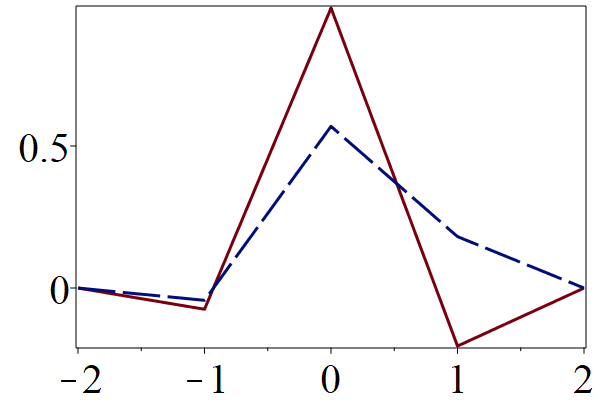
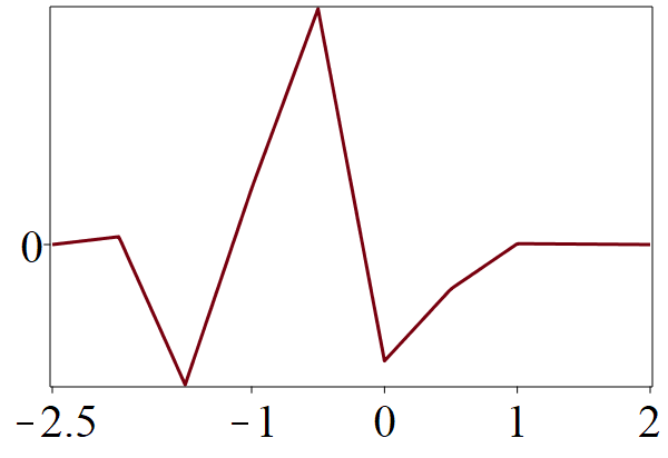
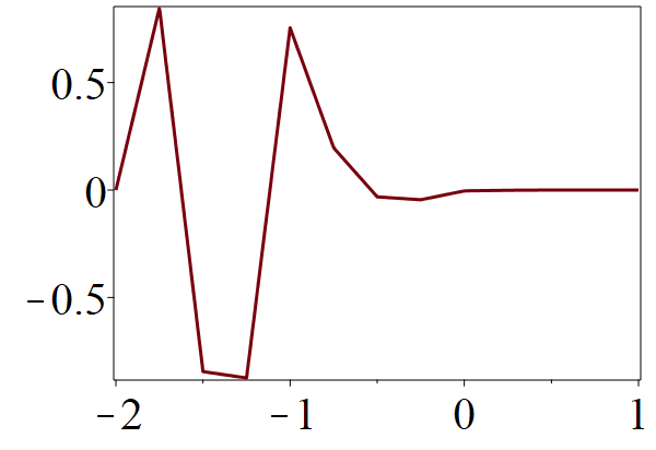
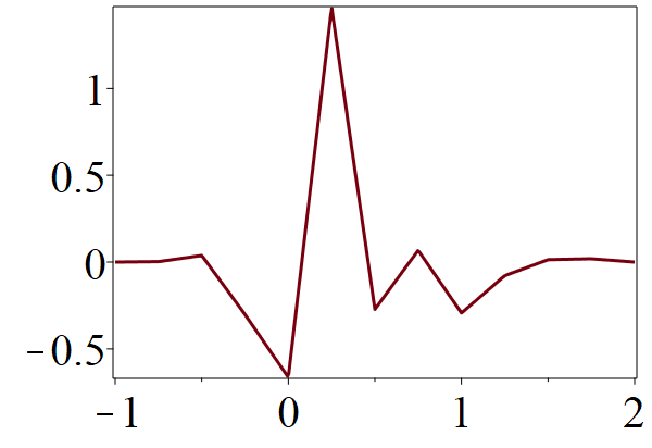
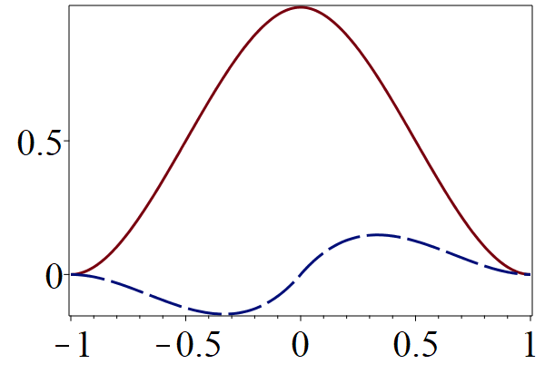
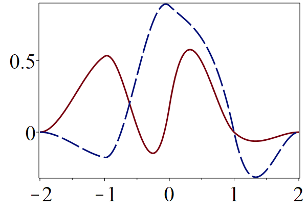
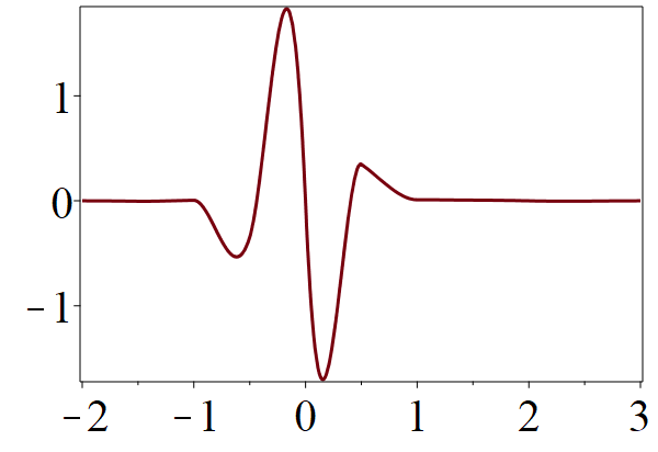
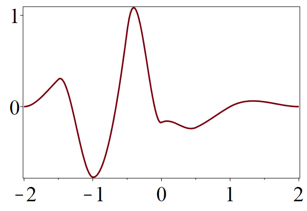
The filter is supported on , i.e., whenever . Define via . Define a new refinable vector function . Then as and is a compactly supported tight -framelet in such that all the desired properties in items (1)–(4) of Theorem 1.2 are satisfied. Note that has vanishing moments. See Figure 2 for graphs of .
As we discussed in item (3) of Lemma 3.2, a -periodic trigonometric polynomial is strongly invertible (i.e., is also a -periodic trigonometric polynomial) if and only if for some and . Thus, as mentioned in Section 3, for framelets constructed from scalar refinable functions to have high vanishing moments, usually it is inevitable to sacrifice the compactness of the associated discrete (scalar) framelet transform, because a non-trivial scalar filter is not strongly invertible. Examples 3 and 4 demonstrate that this difficulty can be easily resolved by simply vectorizing the scalar refinable function, and do the constructions by using the new refinable vector function.
Example 5.
Let be the Hermite cubic splines as defined in (3.14). We have , where is given in (3.15). It is well known that with a matching filter satisfying as . Thus there exist quasi-tight -framelets derived from which satisfy all claims of Theorem 1.2, with the maximum possible choice for balanced vanishing moments. For simplicity of presentation, here we present an example of quasi-tight framelets with instead. Following the construction guidelines, we first construct a desired strongly invertible filter as follows:
Direct computation shows that (5.7) and (5.8) hold with and
We obtain such that is a finitely supported quasi-tight -multiframelet filter bank with , , and . For simplicity of presentation, we write
where denotes the zero matrix and
-
•
is the matrix of -periodic trigonometric polynomials given by
where
-
•
where
-
•
where
-
•
is the matrix of -periodic trigonometric polynomials given by
where
-
•
is the matrix of -periodic trigonometric polynomials given by (6.2).
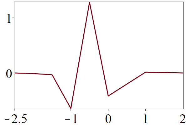
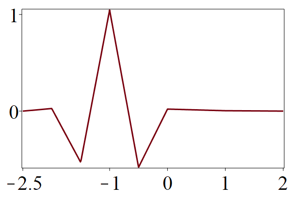
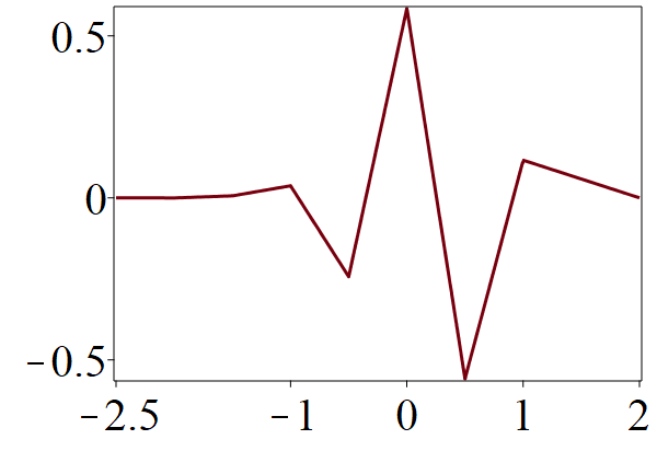
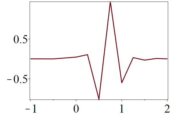
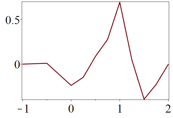
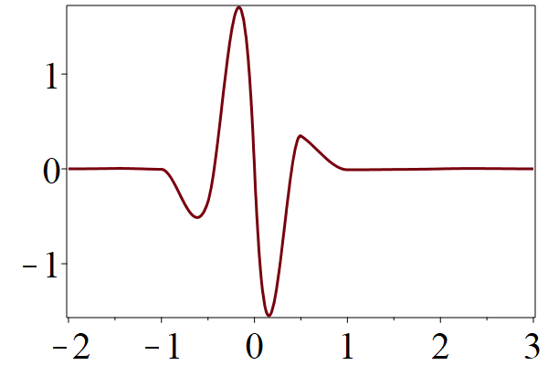
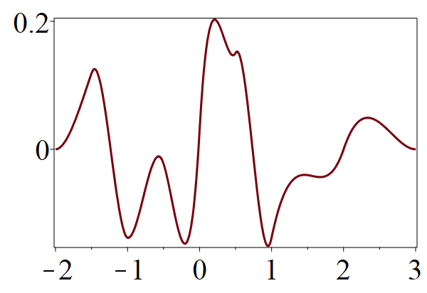
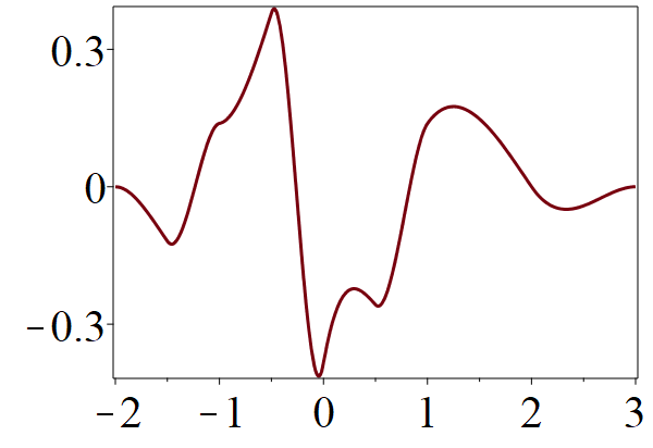
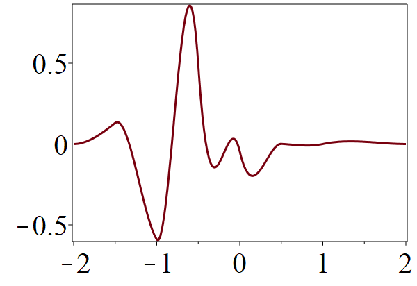
The filter is supported on . Define via . Define a new refinable vector function . Then as and is a compactly supported quasi-tight -framelet in such that all the desired properties in items (1)–(4) of Theorem 1.2 are satisfied with . Note that has vanishing moments. See Figure 3 for graphs of
References
- [1] M. Charina and J. Stöckler, Tight wavelet frames via semi-definite programming. J. Approx. Theory 162 (2010), 1429–1449.
- [2] C. K. Chui and W. He, Compactly supported tight frames associated with refinable functions. Appl. Comput. Harmon. Anal. 8 (2000), 293–319.
- [3] C. K. Chui, W. He, and J. Stöckler, Compactly supported tight and sibling frames with maximum vanishing moments. Appl. Comput. Harmon. Anal. 13 (2002), 224–262.
- [4] C. K. Chui and Q. T. Jiang, Balanced multi-wavelets in , Math. Comp. 74 (2000) 1323–1344.
- [5] I. Daubechies, Ten lectures on wavelets. CBMS-NSF Regional Conference Series in Applied Mathematics, 61. SIAM, 1992.
- [6] I. Daubechies, A. Grossmann and Y. Meyer, Painless nonorthogonal expansions. J. Math. Phys. 27 (1986), 1271–1283.
- [7] I. Daubechies and B. Han, Pairs of dual wavelet frames from any two refinable functions. Constr. Approx. 20 (2004), 325–352.
- [8] I. Daubechies, B. Han, A. Ron, and Z. Shen, Framelets: MRA-based constructions of wavelet frames. Appl. Comput. Harmon. Anal. 14 (2003), 1–46.
- [9] C. Diao and B. Han, Quasi-tight framelets with high vanishing moments derived from arbitrary refinable functions, Appl. Comput. Harmon. Anal., in press. https://doi.org/10.1016/j.acha.2018.12.001.
- [10] C. Diao and B. Han, Generalized matrix spectral factorization and quasi-tight framelets with minimum number of generators, Math. Comp., to appear.
- [11] B. Dong and Z. Shen, MRA-based wavelet frames and applications. Mathematics in Image Processing, 9–158, IAS/Park City Math. Ser., 19, Amer. Math. Soc., Providence, RI, 2013.
- [12] J. S. Geronimo, D. P. Hardin, and P. Massopust, Fractal functions and wavelet expansions based on several scaling functions. J. Approx. Theory 78 (1994), 373–401.
- [13] T. N. T. Goodman, S. L. Lee, and W. S. Tang, Wavelets in wandering subspaces. Trans. Amer. Math. Soc. 338 (1993), 639–654.
- [14] B. Han, On dual wavelet tight frames. Appl. Comput. Harmon. Anal. 4 (1997), 380–413.
- [15] B. Han, Vector cascade algorithms and refinable function vectors in Sobolev spaces. J. Approx. Theory 124 (2003), 44–88.
- [16] B. Han, Dual multiwavelet frames with high balancing order and compact fast frame transform. Appl. Comput. Harmon. Anal. 26 (2009), 14–42.
- [17] B. Han, The structure of balanced multivariate biorthogonal multiwavelets and dual multiframelets. Math. Comp. 79 (2010), 917–951.
- [18] B. Han, Nonhomogeneous wavelet systems in high dimensions. Appl. Comput. Harmon. Anal. 32 (2012), 169–196.
- [19] B. Han, Properties of discrete framelet transforms. Math. Model. Nat. Phenom. 8 (2013), 18–47.
- [20] B. Han, Algorithm for constructing symmetric dual framelet filter banks. Math. Comp. 84 (2015), 767–801.
- [21] B. Han, Framelets and wavelets: Algorithms, analysis, and applications. Applied and Numerical Harmonic Analysis. Birkhäuser/Springer, Cham, 2017. xxxiii + 724 pp.
- [22] B. Han and Q. Mo, Multiwavelet frames from refinable function vectors. Adv. Comput. Math. 18 (2003), 211–245.
- [23] B. Han and Q. Mo, Symmetric MRA tight wavelet frames with three generators and high vanishing moments. Appl. Comput. Harmon. Anal. 18 (2005), 67–93.
- [24] Q. T. Jiang, Symmetric paraunitary matrix extension and parametrization of symmetric orthogonal multifilter banks. SIAM J. Matrix Anal. Appl. 23 (2001), 167–186.
- [25] Q. T. Jiang and Z. Shen, Tight wavelet frames in low dimensions with canonical filters. J. Approx. Theory 196 (2015), 55–78.
- [26] J. Lebrun and M. Vetterli, Balanced multiwavelets: Theory and design. IEEE Trans. Signal Process 46 (1998), 1119–1125.
- [27] Q. Mo, Compactly supported symmetric MTA wavelet frames, Ph.D. thesis at the University of Alberta, (2003).
- [28] Q. Mo, The existence of tight MRA multiwavelet frames. J. Concr. Appl. Math. 4 (2006), 415–433.
- [29] J. Lebrub and M. Vetterli, Balanced multiwavelets: Theory and design, IEEE Trans. Signal Process. 46 (1998) 1119–1125.
- [30] A. Ron and Z. Shen, Affine systems in : the analysis of the analysis operator. J. Funct. Anal. 148 (1997), 408–447.
- [31] I. W. Selesnick, Balanced multiwavelet bases based on symmetric FIR filters, IEEE Trans. Signal Process. 48 (2000) 184–191.
- [32] I. W. Selesnick, Smooth wavelet tight frames with zero moments. Appl. Comput. Harmon. Anal. 10 (2001), 163–181.