Curriculum Labeling: Revisiting Pseudo-Labeling for Semi-Supervised Learning

Abstract

In this paper we revisit the idea of pseudo-labeling in the context of semi-supervised learning where a learning algorithm has access to a small set of labeled samples and a large set of unlabeled samples. Pseudo-labeling works by applying pseudo-labels to samples in the unlabeled set by using a model trained on the combination of the labeled samples and any previously pseudo-labeled samples, and iteratively repeating this process in a self-training cycle. Current methods seem to have abandoned this approach in favor of consistency regularization methods that train models under a combination of different styles of self-supervised losses on the unlabeled samples and standard supervised losses on the labeled samples. We empirically demonstrate that pseudo-labeling can in fact be competitive with the state-of-the-art, while being more resilient to out-of-distribution samples in the unlabeled set. We identify two key factors that allow pseudo-labeling to achieve such remarkable results (1) applying curriculum learning principles and (2) avoiding concept drift by restarting model parameters before each self-training cycle. We obtain $94.91$% accuracy on CIFAR-10 using only $4,000$ labeled samples, and $68.87$% top-1 accuracy on Imagenet-ILSVRC using only 10% of the labeled samples. The code is available at https://github.com/uvavision/Curriculum-Labeling.

1 Introduction

Access to annotated examples has been critical in achieving significant improvements in a wide range of computer vision tasks (Halevy, Norvig, and Pereira 2009; Sun et al. 2017). However, annotated data is typically limited or expensive to obtain. Semi-supervised learning (SSL) methods promise to leverage unlabeled samples in addition to labeled examples to obtain gains in performance. Recent SSL methods for image classification have achieved remarkable results on standard datasets while only relying on a small subset of the labeled data and using the rest as unlabeled data (Tarvainen and Valpola 2017; Miyato et al. 2018; Verma et al. 2019; Berthelot et al. 2019). These methods often optimize a combination of supervised and unsupervised objectives to leverage both labeled and unlabeled samples during training. Our work instead revisits the idea of pseudo-labeling where unlabeled samples are iteratively added into the training data by pseudo-labeling them with a weak model trained on a combination of labeled and pseudo-labeled samples. While pseudo labeling has been proposed before (Lee 2013; Shi et al. 2018; Iscen et al. 2019; Arazo et al. 2019), we revise it by using a self-paced curriculum that we refer to as curriculum labeling, and restarting the model parameters before every iteration in the pseudo-labeling process. We empirically demonstrate through extensive experiments that an implementation of pseudo-labeling trained under curriculum labeling, achieves comparable performance against many other recent methods.

When training a classifier, a common assumption is that the decision boundary should lie in low-density regions in order to improve generalization (Chapelle and Zien 2005); therefore unlabeled samples that lie either near or far from labeled samples should be more informative for decision boundary estimation. Pseudo-labeling generally works by iteratively propagating labels from labeled samples to unlabeled samples using the current model to re-label the data (Scudder 1965; Fralick 1967; Agrawala 1970; Chapelle, Schlkopf, and Zien 2010). Typically, a classifier is first trained with a small amount of labeled data and then used to estimate the labels for all the unlabeled data. High confident predictions are then added as training samples for the next step. This procedure repeats for a specific number of steps or until the classifier cannot find more confident predictions on the unlabeled set. However, pseudo-labeling (Lee 2013; Iscen et al. 2019; Arazo et al. 2019) has been largely surpassed by recent methods (Xie et al. 2019; Berthelot et al. 2019, 2020), and there is little recent work on using this approach for this task.

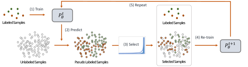
Figure 1: Curriculum Labeling (CL) algorithm. The model is (1) trained on the labeled samples, then this model is used to (2) predict and assign pseudo-labels for the unlabeled samples. Then the distribution of the prediction scores is used to (3) select a subset of pseudo-labeled samples. Then a new model is (4) re-trained with the labeled and pseudo-labeled samples. This process is (5) repeated by re-labeling unlabeled samples using this new model. The process stops when all samples in the dataset have been used during training.

Our work borrows ideas from curriculum learning (Bengio et al. 2009) where a model first uses samples that are easy and progressively moves toward hard samples. Prior work has shown that training with a curriculum improves performance in several machine learning tasks (Bengio et al. 2009; Hacohen and Weinshall 2019). The main challenge in designing a curriculum is how to control the pace – going over the easy examples too fast may lead to more confusion than benefit while moving too slowly may lead to unproductive learning. In particular, we show in our experiments, vanilla handpicked thresholding, as used in previous pseudo-labeling approaches (Oliver et al. 2018), cannot guarantee success out of the box. Instead, we design a self-pacing strategy by analyzing the distribution of the prediction scores of the unlabeled samples and applying a criterion based on Extreme Value Theory (EVT) (Clifton, Hugueny, and Tarassenko 2011). Figure 1 shows an overview of our model. We empirically demonstrate that curriculum labeling can achieve competitive results in comparison to the state-of-the-art, matching the recently proposed UDA (Xie et al. 2019) on Imagenet and surpassing UDA (Xie et al. 2019) and ICT (Verma et al. 2019) on CIFAR-10.

A current issue in the evaluation of SSL methods was recently highlighted by Oliver et al (Oliver et al. 2018), which criticize the widespread practice of setting aside a small part of the training data as “labeled” and a large portion of the same training data as “unlabeled”. This way of splitting the data leads to a scenario where all images in this type of “unlabeled” set have the implicit guarantee that they are drawn from the exact same class distribution as the “labeled” set. As a result, several SSL methods underperform under the more realistic scenario where unlabeled samples do not have this guarantee. We demonstrate that pseudo-labeling under a curriculum is surprisingly robust to out-of-distribution samples in the unlabeled set compared to other methods.

Our contributions can be summarized as follows:

• We propose curriculum labeling (CL), which augments pseudo-labeling with a careful curriculum choice as pacing criteria based on Extreme Value Theory (EVT).

• We demonstrate that, with the proposed curriculum paradigm, the classic pseudo-labeling approach can deliver near state-of-the-art results on CIFAR-10, Imagenet ILSVRC top-1 accuracy, and SVHN – compared to very recently proposed methods.

• Additionally, compared to previous approaches, our version of pseudo-labeling leads to more consistent results in realistic evaluation settings, where out-of-distribution samples are present.

2 Related Work

Our work is most closely related to the general use of pseudo-labeling in semi supervised learning (Lee 2013; Shi et al. 2018; Iscen et al. 2019; Arazo et al. 2019). Although these methods have been surpassed by consistency regularization methods, our work suggests that this is not a fundamental flaw of self-training algorithms and demonstrate that careful selection of thresholds and pacing of the pseudo-labeling of the unlabeled samples can lead to significant gains. Here (Lee 2013; Shi et al. 2018; Arazo et al. 2019) relied on a trained parametric model to pseudo-label unlabeled samples (e.g. by choosing the most confident class (Lee 2013; Shi et al. 2018), or using soft-labels (Arazo et al. 2019)), while (Iscen et al. 2019) proposed to propagate labels using a nearest-neighbors graph. Unlike these methods we adopt curriculum labeling which adds self-pacing to our training where we only add the most confident samples in the first few iterations and the threshold is chosen based on the distribution of scores on training samples.

Most closely related to our approach is the concurrent work of Arazo et al (Arazo et al. 2019) where pseudo-labeling is adopted in combination with Mixup (Zhang et al. 2018) to prevent what is referred in that work as confirmation bias. Confirmation bias is related in this context to the phenomenon of concept drift where the properties of a target variable change over time. This deserves special attention in pseudo-labeling since the target variables are affected by the same model feeding onto itself. In our version of pseudo-labeling we alleviate this confirmation bias by re-initializing the model before every self-training iteration, and as such, pseudo-labels from past epochs do not have an outsized effect on the final model. While our results are comparable on CIFAR-10, the work of Arazo et al (Arazo et al. 2019) further solidifies our finding that pseudo-labeling has a lot more to offer than previously found.

Recent methods for semi-supervised learning rather use a consistency regularization approach. In these works (Sajjadi, Javanmardi, and Tasdizen 2016; Laine and Aila 2017; Tarvainen and Valpola 2017; Sohn et al. 2020), a network is trained to make consistent predictions in response to perturbation of unlabeled samples, by combining the standard cross-entropy loss with a consistency loss. Consistency losses generally encourage that in the absence of labels for a sample, its predictions should be consistent with the predictions for a perturbed version of the same sample. Various perturbation operations have been explored, including basic image processing operators (Xie et al. 2019), dedicated operators such as MixUp (Zhang et al. 2018; Berthelot et al. 2020), learned transformations (Cubuk et al. 2018), and adversarial perturbations (Miyato et al. 2018). While we optionally leverage data augmentation, our use of it is the same as in the standard supervised setting, and our method does not enforce any consistency for pairs of samples.

3 Method: Pseudo-Labeling under Curriculum

In semi-supervised learning (SSL), a dataset $D=\{x|x\in X\}$ is comprised of two disjoint subsets: a labeled subset $D_{L}=\{(x,y)|x\in X,y\in Y\}$ and an unlabeled subset $D_{UL}=\{x|x\in X\}$, where $x$ and $y$ denote the input and the corresponding label. Typically $|D_{L}|\ll|D_{UL}|$.

Pseudo-labeling builds upon the general self-training framework (McLachlan 1975), where a model goes through multiple rounds of training by leveraging its own past predictions. In the first round, the model is trained on the labeled set $D_{L}$. In all subsequent rounds, the training data is the union of $D_{L}$ and a subset of $D_{UL}$ pseudo-labeled by the model in the previous round. In round $t$, let the training samples be denoted as $(X_{t},Y_{t})$ and the current model as $P_{\theta}^{t}$, where $\theta$ are the model parameters, and $t\in\{1,\cdots,T\}$. After round $t$, an unlabeled subset $\bar{X_{t}}$ is added into $X_{t+1}:=X_{1}\cup\bar{X_{t}}$, and the new target set is defined as $Y_{t+1}:=Y_{1}\cup\bar{Y_{t}}$. Here $\bar{Y_{t}}$ represents the pseudo labels of $\bar{X_{t}}$, predicted by model $P_{\theta}^{t}$. In this sense, the labels are “propagated” to the unlabeled data points via $P_{\theta}^{t}$.

The criterion used to decide which subset of samples in $D_{UL}$ to incorporate into the training in each round is key to our method. Different uncertainty metrics have been explored in the previous literature, including choosing the samples with the highest-confidence (Zhu 2006), or retrieving the nearest samples in feature space (Shi et al. 2018; Iscen et al. 2019; Luo et al. 2017). We draw insights from Extreme Value Theory (EVT) which is often used to simulate extreme events in the tails of one-dimensional probability distributions by assessing the probability of events that are more extreme (Broadwater and Chellappa 2010; Rudd et al. 2018; Al-Behadili, Grumpe, and Wöhler 2015; Clifton et al. 2008; Shi et al. 2008). In our problem, we observed that the distribution of the maximum probability predictions for pseudo-labeled data follows this type of Pareto distribution. So instead of using fixed thresholds or tuning thresholds manually, we use percentile scores to decide which samples to add. Algorithm 1 shows the full pipeline of our model, where $\textit{Percentile}(X,T_{r})$ returns the value of the $r$-th percentile. We use values of $r$ from 0% to 100% in increments of 20.

Algorithm 1 Pseudo-Labeling under Curriculum Labeling

1:Require: $D_{L}$ $\triangleright$ set of labeled samples

2:Require: $D_{UL}$ $\triangleright$ set of unlabeled samples

3:Require: $\Delta:=20$ $\triangleright$ stepping threshold percent

4:$P_{\theta}^{t}$ $\leftarrow$ train classifier using $D_{L}$ only

5:$t:=1$

6:$T_{r}:=100-\Delta$

7:do

8:     $T:=\textit{Percentile}(P_{\theta}^{t}(D_{UL}),T_{r})$

9:     $X_{t}:=D_{L}$

10:     for $x\in D_{UL}$ do

11:         if $P_{\theta}^{t}(x)$ $>$ $T$ then

12:               $X_{t}:=X_{t}\cup{(x,\textit{pseudo-label}(P_{\theta}^{t},x))}$               

13:     $P_{\theta}^{t}$ $\leftarrow$ train classifier from scratch using $X_{t}$

14:     $t:=t+1$

15:     $T_{r}:=T_{r}-\Delta$

16:while $|X_{t}|\neq|D_{L}+D_{UL}|$

17:end

Note that, in Algorithm 1 $\bar{X_{t}}$ is selected from the whole unlabeled set $D_{UL}$, enabling previous pseudo-annotated samples to enter or to leave the new training set. This is used to discourage concept drift or confirmation bias, as it can prevent erroneous labels predicted by an undertrained network during the early stages of training to be accumulated. To further alleviate the problem, we also reinitialize the model parameters $\theta$ with random initializations after each round, and empirically observe that, –as opposed to fine-tuning–, our reinitialization strategy leads to better performance.

Our termination criteria is that we keep iterating until all the samples in the pseudo-labeled set comprise the entire training data samples which will take place when the percentile threshold is lowered to the minimum value ($T_{r}=0$).

4 Theoretical Analysis

Our data consists of $N$ labeled examples $(X_{i},Y_{i})$ and $M$ examples $X_{j}$ which are unlabeled. Let $\mathcal{H}$ be a set of hypotheses $h_{\theta}$ where $h_{\theta}\in\mathcal{H}$, and each of them denotes a function mapping $X$ to $Y$. Let $L_{\theta}(X_{i})$ denote the loss for a given example $X_{i}$. To choose the best predictor with the lowest possible error, our formulation can be explained with a regularized Empirical Risk Minimization (ERM) framework. Below, we define $\mathcal{L}(\theta)$ as the pseudo-labeling regularized empirical loss as:

$$\begin{split}&\mathcal{L}(\theta)=\hat{\mathbb{E}}[L_{\theta}]=\frac{1}{N}\sum_{i=1}^{N}L_{\theta}(X_{i})+\frac{1}{M}\sum_{j=1}^{M}L^{\prime}_{\theta}(X_{j})\\ &\hat{\theta}=\operatorname*{arg\,min}_{\theta}\mathcal{L}(\theta)\\ &L_{\theta}(X_{i})=\texttt{CEE}(P_{\theta}^{t}(X_{i}),Y_{i})\\ &L^{\prime}_{\theta}(X_{j})=\texttt{CEE}(P_{\theta}^{t}(X_{j}),P_{\theta}^{t-1}(X_{j}))\end{split}$$ (1)

Here CEE indicates cross entropy. Following (Hacohen and Weinshall 2019) this can be rewritten as follows:

$$\begin{split}&\hat{\theta}=\operatorname*{arg\,min}_{\theta}\mathcal{L}(\theta)=\operatorname*{arg\,max}_{\theta}\exp(-\mathcal{L}(\theta))\end{split}$$ (2)

Now to simplify the notions, we reformulate the objective as to maximize a so-called Utility objective, where $\delta$ is an indicator function:

$$\begin{split}&U_{\theta}(X)=e^{-\delta(X\in L)L_{\theta}(X)-\delta(X\in UL)L^{\prime}_{\theta}(X)}\\ &\mathcal{U}(\theta)=\hat{\mathbb{E}}[U_{\theta}]=\frac{1}{N}\sum_{i=1}^{N}U_{\theta}(X_{i})+\frac{1}{M}\sum_{i=1}^{M}U^{\prime}_{\theta}(X_{j})\\ \end{split}$$ (3)

The pacing function in our pseudo curriculum labeling effectively provides a Bayesian prior for sampling unlabeled samples. This can be formalized as follows:

$$\mathcal{U}_{p}(\theta)=\hat{\mathbb{E}}_{p}[U_{\theta}]=\frac{1}{N}\sum_{i=1}^{N}U_{\theta}(X_{i})+\sum_{j=1}^{M}U^{\prime}_{\theta}(X_{j})p(X_{j})$$

$$=\frac{1}{N}\sum_{i=1}^{N}U_{\theta}(X_{i})+\sum_{j=1}^{M}e^{-L^{\prime}_{\theta}(X_{j})}p_{j}$$

$$\hat{\theta}=\operatorname*{arg\,max}_{\theta}\mathcal{U}_{p}(\theta)$$ (4)

Here $p_{j}=p(X_{j})$ denotes the induced prior probability we use to decide how to sample the unlabeled samples and is determined by the pacing function of curriculum labeling algorithm, thus, $p(X_{j})$ works like an indicator function where $1/M$ are the unlabeled samples whose scores are in the top $\mu$ percentile, and 0 otherwise.

We can then rewrite part of Eq (4) as follows

$$\begin{split}\mathcal{U}_{p}(\theta)&=\frac{1}{N}\sum_{i=1}^{N}U_{\theta}(X_{i})+\sum_{j=1}^{M}(U^{\prime}_{\theta}(X_{j})-\hat{\mathbb{E}}[U^{\prime}_{\theta}])(p_{j}-\hat{\mathbb{E}}[p])\\ &\hskip 12.80365pt+M*\hskip 1.0pt\hat{\mathbb{E}}[U^{\prime}_{\theta}]\hat{\mathbb{E}}[p]\\ &=\frac{1}{N}\sum_{i=1}^{N}U_{\theta}(X_{i})+\hat{\mathrm{Cov}}[U^{\prime}_{\theta},p]+M*\hskip 1.0pt\hat{\mathbb{E}}[U^{\prime}_{\theta}]\hat{\mathbb{E}}[p]\\ &=\mathcal{U}(\theta)+\hat{\mathrm{Cov}}[U^{\prime}_{\theta},p]\end{split}$$ (5)

Eq (5) tells that when we sample the unlabeled data points according to a probability that positively correlates with the confidence of the predictions of $X_{j}$ (negative correlating with the loss $L^{\prime}(X_{j})$), we are improving the utility of the estimated $\theta$. Under such a pacing curriculum, we are minimizing the overall loss $\mathcal{L}$. The smaller the $L^{\prime}(X_{j})$ (the larger the utility of an unlabeled point $X_{j}$), the more likely we sample $X_{j}$. This theoretically proves that we want to sample more those unlabeled points that are predicted with more confidence.

5 Experiments

We first discuss our experiment settings in detail, then we compare against previous methods using the standard semi-supervised learning practice of setting aside a portion of the training data as labeled, and the rest as unlabeled, then we test in the more realistic scenario where unlabeled training samples do not follow the same distribution as labeled training samples, finally we conduct extensive evaluation justifying why our version of pseudo-labeling and specifically curriculum labeling enables superior results compared to prior efforts on pseudo-labeling.

5.1 Experimental Settings

Datasets: We evaluate the proposed approach on three image classification datasets: CIFAR-10 (Krizhevsky 2012), Street View House Numbers (SVHN) (Netzer et al. 2011), and ImageNet ILSVRC (Russakovsky et al. 2015; Deng et al. 2009). With CIFAR-10 we use 4,000 labeled samples and 46,000 unlabeled samples for training and validation, and evaluate on 10,000 test samples. We also report results when the training set is restricted to 500, 1,000, and 2,000 labeled samples. With SVHN we use 1,000 labeled samples and 71,257 unlabeled samples for training, 1,000 samples for validation, which is significantly lower than the conventional 7,325 samples generally used, and evaluate on 26,032 test samples. With ImageNet we use $\sim$10% of the dataset as labeled samples (102,000 for training and 26,000 for validation), 1,253,167 unlabeled samples and 50,000 test samples.

Model Details: We use CNN-13 (Springenberg et al. 2014) and WideResNet-28 (Zagoruyko and Komodakis 2016) (depth 28, width 2) for CIFAR-10 and SVHN, and ResNet-50 (He et al. 2015) for ImageNet. The networks are optimized using Stochastic Gradient Descent with nesterov momentum. We use weight decay regularization of 0.0005, momentum factor of 0.9, and an initial learning rate of 0.1 which is then updated by cosine annealing (Loshchilov and Hutter 2016). Note that we use the same hyper-parameter setting for all of our experiments, except the batch size when applying moderate and heavy data augmentation. We empirically observe that small batches (i.e. 64-100) work better for moderate data augmentation (random cropping, padding, whitening and horizontal flipping), while large batches (i.e. 512-1024) work better for heavy data augmentation. For CIFAR-10 and SVHN, we train the models for 750 epochs. Starting from the 500th epoch, we also apply stochastic weight averaging (SWA) (Izmailov et al. 2018) every 5 epochs. For ImageNet, we train the network for 220 epochs and apply SWA, starting from the 100th epoch.

Data Augmentation: While data augmentation has became a common practice in supervised learning especially when the training data is scarce (Simard, Steinkraus, and Platt 2003; Perez and Wang 2017; Shorten and Khoshgoftaar 2019; Devries and Taylor 2017), previous work on SSL typically use basic augmentation operations such as cropping, padding, whitening and horizontal flipping (Rasmus et al. 2015; Laine and Aila 2017; Tarvainen and Valpola 2017). More recent work relies on heavy data augmentation policies that are learned automatically by Reinforcement Learning (Cubuk et al. 2018) or density matching (Lim et al. 2019). Other augmentation techniques generate perturbations that take the form of adversarial examples (Miyato et al. 2018), or by interpolations between a random pair of image samples (Zhang et al. 2018). We explore both moderate and heavy data augmentation techniques that do not require to learn or search any policy, but instead apply transformations in an entirely random fashion. We show that using arbitrary transformations on the training set yields positive results. We refer to this technique as Random Augmentation (RA) in our experiments. However, we also report results without the use of data augmentation.

Approach	Method	Year	CIFAR-10	SVHN
			$N_{l}$ = 4000	$N_{l}$ = 1000
–	Supervised	–	20.26 $\pm$ 0.38	12.83 $\pm$ 0.47
Pseudo Labeling	PL (Lee 2013)	2013	17.78 $\pm$ 0.57	7.62 $\pm$ 0.29
	PL-CB (Arazo et al. 2019)	2019	6.28 $\pm$ 0.3	-
Consistency Regularization	$\Pi$ Model (Laine and Aila 2017)	2017	16.37 $\pm$ 0.63	7.19 $\pm$ 0.27
	Mean Teacher (Tarvainen and Valpola 2017)	2017	15.87 $\pm$ 0.28	5.65 $\pm$ 0.47
	VAT (Miyato et al. 2018)	2018	13.86 $\pm$ 0.27	5.63 $\pm$ 0.20
	VAT + EntMin (Miyato et al. 2018)	2018	13.13 $\pm$ 0.39	5.35 $\pm$ 0.19
	LGA + VAT (Jackson and Schulman 2019)	2019	12.06 $\pm$ 0.19	6.58 $\pm$ 0.36
	ICT (Verma et al. 2019)	2019	7.66 $\pm$ 0.17	3.53 $\pm$ 0.07
	MixMatch (Berthelot et al. 2019)	2019	6.24 $\pm$ 0.06	3.27 $\pm$ 0.31
	UDA (Xie et al. 2019)	2019	5.29 $\pm$ 0.25	2.46 $\pm$ 0.17
	ReMixMatch (Berthelot et al. 2020)	2020	5.14 $\pm$ 0.04	2.42 $\pm$ 0.09
	FixMatch (Sohn et al. 2020)	2020	4.26 $\pm$ 0.05	2.28 $\pm$ 0.11
Pseudo Labeling	CL	2020	8.92 $\pm$ 0.03	5.65 $\pm$ 0.11
	CL+FA(Lim et al. 2019)	2020	5.51 $\pm$ 0.14	2.90 $\pm$ 0.19
	CL+FA(Lim et al. 2019)+Mixup(Zhang et al. 2018)	2020	5.09 $\pm$ 0.18	2.75 $\pm$ 0.15
	CL+RA+Mixup(Zhang et al. 2018)	2020	5.27 $\pm$ 0.16	2.80 $\pm$ 0.18

Table 1: Test error rate on CIFAR-10 and SVHN using WideResNet-28. We show that our CL method can achieve comparable results to the state-of-the-art. ”Supervised” refers to using only 4,000/1,000 labeled samples from CIFAR-10/SVHN without relying on any unlabeled data.

Approach	Method	CIFAR-10	SVHN
		$N_{l}$ = 4000	$N_{l}$ = 1000
Pseudo Labeling	TSSDL-MT (Shi et al. 2018)	9.30 $\pm$ 0.55	3.35 $\pm$ 0.27
	LP-MT (Iscen et al. 2019)	10.61 $\pm$ 0.28	-
Consistency Regularization	Ladder net (Rasmus et al. 2015)	12.36 $\pm$ 0.31	–
	MeanTeacher (Tarvainen and Valpola 2017)	12.31 $\pm$ 0.24	3.95 $\pm$ 0.19
	Temporal ensembling (Laine and Aila 2017)	12.16 $\pm$ 0.24	4.42 $\pm$ 0.16
	VAT (Miyato et al. 2018)	11.36 $\pm$ 0.34	5.42
	VAT+EntMin (Miyato et al. 2018)	10.55 $\pm$ 0.05	3.86
	SNTG (Luo et al. 2017)	10.93 $\pm$ 0.14	3.86 $\pm$ 0.27
	ICT (Verma et al. 2019)	7.29 $\pm$ 0.02	2.89 $\pm$ 0.04
Pseudo Labeling	CL	9.81 $\pm$ 0.22	4.75 $\pm$ 0.28
	CL+RA	5.92 $\pm$ 0.07	3.96 $\pm$ 0.10

Table 2: Test error rate on CIFAR-10 and SVHN using CNN-13. The value $N_{l}$ stands for the number of labeled examples in the training set.

5.2 Comparisons with the State-of-the-Art

CIFAR-10/SVHN: In Table 1 and 2, we compare different versions of our method with state-of-the-art approaches using the WideResnet-28/CNN-13 architectures on CIFAR-10 and SVHN. Our method surprisingly surpasses previous pseudo-labeling based methods (Lee 2013; Shi et al. 2018; Iscen et al. 2019; Arazo et al. 2019) and consistency-regularization methods (Xie et al. 2019; Berthelot et al. 2019, 2020) on CIFAR-10. In SVHN we obtain competitive test error when compared with all previous methods that rely on moderate augmentation (Lee 2013; Rasmus et al. 2015; Laine and Aila 2017; Tarvainen and Valpola 2017; Luo et al. 2017), moderate-to-high data augmentation (Miyato et al. 2018; Jackson and Schulman 2019; Verma et al. 2019; Berthelot et al. 2019), and heavy data augmentation (Xie et al. 2019).

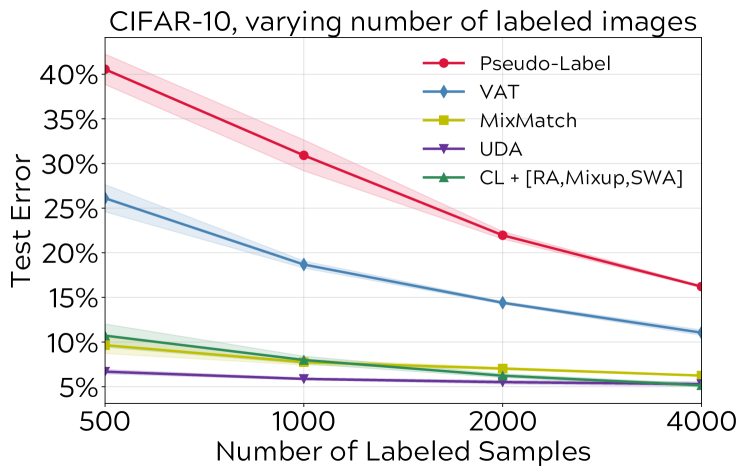
Figure 2: Comparison of test error rate using WideResNet varying the size of the labeled samples on CIFAR-10. We use the standard validation set size of 5,000 to make our method comparable with previous work.

A common practice to test SSL algorithms, is to vary the size of the labeled data using 50, 100 and 200 samples per class. In Figure 2, we also evaluate our method using this setting on WideResNet for CIFAR-10. We use the standard validation set size of 5,000 to make our method comparable with previous work. Decreasing the size of the available labeled samples recreates a more realistic scenario where there is less labeled data available. We keep the same hyperparameters we use when training on 4,000 labeled samples, which shows that our model does not drastically degrade when dealing with smaller labeled sets. We show the lines for the mean and shaded regions for the standard deviation across five independent runs, and our results are closer to the current best method under this benchmark UDA (Xie et al. 2019).

ImageNet: We further evaluate our method on the large-scale ImageNet dataset (ILSVRC). Following prior works (Verma et al. 2019; Xie et al. 2019; Berthelot et al. 2019), we use 10%/90% of the training split as labeled/unlabeled data. Table 3 shows that we achieve competitive results with the state-of-the-art with scores very close to the current top performing method, UDA (Xie et al. 2019) on both top-1 and top-5 accuracies.

Method	Approach	Top-1	Top-5
Supervised Baseline (Zhai et al. 2019)	–	–	80.43
Pseudo-Label (Lee 2013)	Pseudo Labeling	–	82.41
VAT (Miyato et al. 2018)	Consist. Reg.	–	82.78
VAT + EntMin (Miyato et al. 2018)	Consist. Reg.	–	83.39
$S^{4}$ $L$-Rotation (Zhai et al. 2019)	Self-Supervision	–	83.82
$S^{4}$ $L$-Exemplar (Zhai et al. 2019)	Self-Supervision	–	83.72
UDA Supervised (Xie et al. 2019)	–	55.09	77.26
UDA Supervised (w. Aug) (Xie et al. 2019)	–	58.84	80.56
UDA (w. Aug) (Xie et al. 2019)	Consist. Reg.	68.78	88.80
FixMatch (Sohn et al. 2020)	Consist. Reg. + PL	71.46	89.13
CL Supervised (w. Aug)	–	55.75	79.67
CL (w. Aug)	Pseudo Labeling	68.87	88.56

Table 3: Top-1 and top-5 accuracies on ImageNet with 10% of the labeled set. Here UDA and CL are trained using ResNet-50. Previous methods (Lee 2013; Miyato et al. 2018; Zhai et al. 2019) use ResNet-50v2 to report their results.

5.3 Realistic Evaluation with Out-of-Distribution Unlabeled Samples

In a more realistic SSL setting (Oliver et al. 2018), the unlabeled data may not share the same class set as the labeled data. We test our method under a scenario where the labeled and unlabeled data come from the same underlying distribution, but the unlabeled data contains classes not present in the labeled data as proposed by (Oliver et al. 2018). We reproduce the experiment by synthetically varying the class overlap on CIFAR-10, choosing only the animal classes to perform the classification (bird, cat, deer, dog, frog, horse). In this setting, the unlabeled data comes from four classes. The idea is to vary how many of those classes are among the six animal classes to modulate the class distribution mismatch. We report the results of (Lee 2013; Miyato et al. 2018) from (Oliver et al. 2018). We also include the results of (Verma et al. 2019; Xie et al. 2019) obtained by running their released source code. Figure 3 shows that our method is robust to out-of-distribution classes, while the performance of previous methods drops significantly. We conjecture that our self-pacing curriculum is key to this scenario, where the adaptive thresholding scheme could help filter the out-of-distribution unlabeled samples during training.

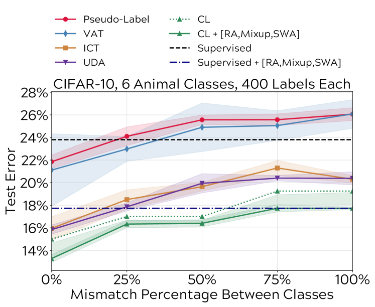
Figure 3: Comparison of test error on CIFAR-10 (six animal classes) with varying overlap between classes. For example, in “50%”, two of the four classes in the unlabeled data are not present in the labeled data. “Supervised” refers to using only the 2,400 labeled images.

5.4 Ablation Studies

Here we justify the effectiveness of the two main design differences in our version of pseudo-labeling with respect to previous attempts. We first demonstrate that the choice of thresholds using percentiles as in curriculum labeling, has a large effect on the results compared to fixed thresholds, then we show that training the model parameters from scratch in each round of self-training is more beneficial than fine-tuning over previous versions of the model.

Data Augmentation	Mixup	SWA	Top-1 Error
None	✗	✗	38.47
None	✓	✗	34.03
None	✗	✓	37.35
None	✓	✓	32.85
Moderate	✗	✗	22.8
Moderate	✓	✗	16.11
Moderate	✗	✓	21.63
Moderate	✓	✓	15.83
Heavy (RA)	✗	✗	11.38
Heavy (RA)	✓	✗	8.88
Heavy (RA)	✗	✓	11.32
Heavy (RA)	✓	✓	8.59

Table 4: Test errors when using pseudo-labeling without a curriculum (the threshold is set to 0.0). We use WideResnet-28 as the base network. Additionally, we report which data augmentation technique was applied.

Threshold	Moderate Aug	Heavy (RA)
0.1	21.12	7.87
0.2	21.12	8.57
0.3	20.59	7.90
0.4	22.11	8.15
0.5	19.98	7.46
0.6	19.51	6.88
0.7	19.35	6.65
0.8	18.08	6.29
0.9	17.11	6.21
CL	8.92	5.27

Table 5: Test errors when using pseudo-labeling with several fixed thresholds and different data augmentation techniques. We use WideResnet-28 as the base network. The Heavy Augmentation applies Random Augmentation, Mixup and SWA. Last row shows results of our approach under the proposed curriculum criteria.

Effectiveness of Curriculum Labeling

	0.9 1 #	WRN1	0.9995 2 #	WRN2	Self-pacing #	WRN
Fully Supervised	-	18.25	-	18.25	-	18.25
1º Iteration	$\sim$35k	15.25	$\sim$13k	17.18	8k	15.41
2º Iteration	$\sim$41k	14.53	$\sim$14k	15.2	16k	11.55
3º Iteration	$\sim$43k	13.91	$\sim$14k	14.64	24k	10.83
4º Iteration	$\sim$44k	14.01	$\sim$17k	14.84	32k	9.54
5º Iteration	$\sim$44k	12.92	$\sim$15k	15.29	41k	8.92

Table 6: Test errors when using two static thresholds (0.9¹ and 0.9995²) and our self-pacing training. We use WideResnet-28(WRN) as the base network. Fully Supervised refers to using only 4,000 labeled datapoints from CIFAR-10 without any unlabeled data. The # columns show the average numbers of images automatically selected for each iteration during training. We used ZCA preprocessing and moderate data augmentation on these experiments.

	Top			Fine
	Confidence	#	Reinitializing	Tuning
Fully Supervised	-	-	15.42	15.3
1º Iteration	$80\%$	8k	10.04	9.85
2º Iteration	$60\%$	16k	8.56	7.99
3º Iteration	$40\%$	24k	7.03	7.20
4º Iteration	$20\%$	32k	6.22	6.55
5º Iteration	$0\%$	41k	5.41	6.42

Table 7: Comparison of model reinitialization and finetuning, in each iteration of training. We observe that reinitializing the model performs consistently better in each iteration.

We first show results when applying vanilla pseudo-labeling with no curriculum, and without a specific threshold (i.e. 0.0). Table 5 shows the effect when applying different data augmentation techniques (Random Augmentation, Mixup and SWA). We show that only when heavy data augmentation is used, this approach is able to match our curriculum design without any data augmentation. This vanilla pseudo-labeling approach is similar to the one reported in previous literature (Lee 2013), and is not able to outperform recent work based on consistency regularization techniques. We also report experiments applying smaller thresholds in each iteration, and show our results in table 5. Our curriculum design is able to yield a significant gain over the traditional pseudo-labeling approach that uses a fixed threshold even when heavy data augmentation is applied. This shows that our curriculum approach is able to alleviate the concept drift and confirmation bias.

Then we compare our self-pacing curriculum labeling with handpicked thresholding mimicking the experiments presented in Oliver et al (Oliver et al. 2018) and report more detailed results per iteration. As performed in this earlier work, we re-label only the most confident samples; in our experiments we fixed the thresholds to 0.9 and 0.9995. We test on CIFAR-10 with 4000 labeled samples, and use WideResnet-28 as the base network with moderate data augmentation. As shown in Table 6, using handpicked thresholds is sub-optimal. Especially when only the most confident samples are re-labeled as in (Lee 2013). Particularly, there is little to no improvement after the first iteration. Our self-pacing model significantly outperforms fixed thresholding and continues making progress in different iterations.

Effectiveness of Reinitializing vs Finetuning

Due to the confirmation bias and concept drift, errors caused by high confident mis-labeling in early iterations may accumulate during multiple rounds of training. Although our self-pacing sample selection encourages excluding incorrectly labeled samples in early iterations, this might still be an issue. As such, we decided to reinitialize the model after each iteration, instead of finetuning the previous model. Reinitializing the model yields at least 1% improvement and does not add a significant overhead to our self-paced approach, which is significantly faster than recent methods (additional experiments in the Appendix). In Table 7, we compare the performance of model reinitializing and finetuning on CIFAR-10 on the 4,000 labeled training samples regime. We use WideResnet-28 as the base network and apply data augmentation during training. It shows that reinitializing the model, as opposed to finetuning, indeed improves the accuracy significantly, demonstrating an alternative and perhaps simpler solution to alleviate the issue of confirmation bias (Arazo et al. 2019).

6 Conclusion

In this paper, we revisit pseudo-labeling in the context of semi-supervised learning and demonstrate comparable results with the current state-of-the-art that mostly relies on enforcing consistency on the predictions for unlabeled samples. As part of our version of pseudo-labeling, we propose curriculum labeling where unlabeled samples are chosen by using a threshold that accounts for the skew in the distribution of the prediction scores on the unlabeled samples. We additionally show that concept drift and confirmation bias can be mitigating by discarding the current model parameters before each epoch in the self-training loop of pseudo-labeling. We demonstrate our findings with strong empirical results on CIFAR-10, SVHN, and ImageNet ILSVRC.

Acknowledgments Part of this work was supported by generous funding from SAP Research. We also thank anonymous reviewers for their feedback.

Appendix A Appendix

A.1 Decision boundaries when applying Pseudo-Labeling and Curriculum Labeling

We show in Figure 4 how curriculum labeling works on the synthetic two-moon dataset as it progressively labels the unlabeled samples. We observe that unlabeled samples get progressively labeled mostly with their correct labels as learning progresses.

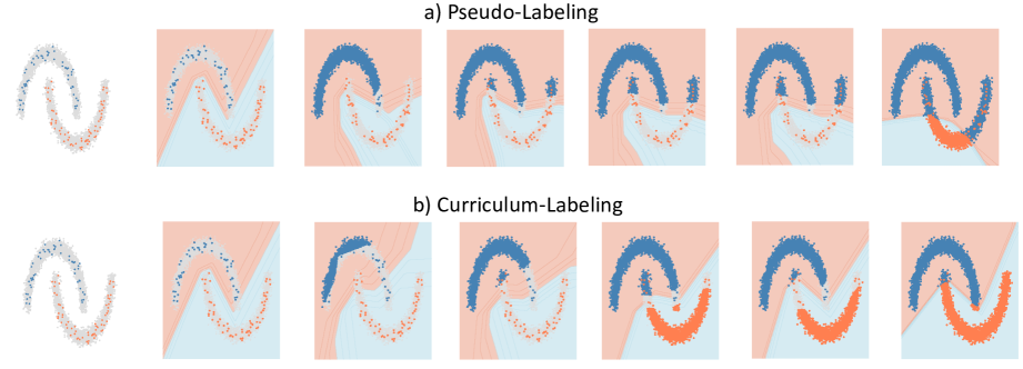
Figure 4: Comparison of regular pseudo-labeling (PL) (Lee 2013) and pseudo-labeling with curriculum labeling (CL) on the “two moons” synthetic dataset. In blue are positive samples, in orange are negative samples, and in gray are unlabeled samples. Subsequent plots show how the learned decision boundaries evolve during training for the two approaches, showing that a self-paced approach leads to a more desirable state.

A.2 Theoretical Analysis Derivation

The derivation of Eq (5) in the Theoretical Analysis (section 4) is as follows:

$$\begin{split}\sum_{j=1}^{M}U^{\prime}_{\theta}(X_{j})p(X_{j})=\sum_{j=1}^{M}U^{\prime}_{\theta}(X_{j})p(X_{j})-M*\hat{\mathbb{E}}[U^{\prime}_{\theta}]\hat{\mathbb{E}}[p]\\ -M*\hat{\mathbb{E}}[U^{\prime}_{\theta}]\hat{\mathbb{E}}[p]+M*\hat{\mathbb{E}}[U^{\prime}_{\theta}]\hat{\mathbb{E}}[p]+M*\hat{\mathbb{E}}[U^{\prime}_{\theta}]\hat{\mathbb{E}}[p]\\ =\sum_{j=1}^{M}U^{\prime}_{\theta}(X_{j})p(X_{j})-\sum_{j=1}^{M}\hat{\mathbb{E}}[U^{\prime}_{\theta}]p(X_{j})\\ -\sum_{j=1}^{M}U^{\prime}_{\theta}(X_{j})\hat{\mathbb{E}}[p]+\sum_{j=1}^{M}\hat{\mathbb{E}}[U^{\prime}_{\theta}]\hat{\mathbb{E}}[p]+M*\hat{\mathbb{E}}[U^{\prime}_{\theta}]\hat{\mathbb{E}}[p]\\ =\sum_{j=1}^{M}(U^{\prime}_{\theta}(X_{j})p(X_{j})-\hat{\mathbb{E}}[U^{\prime}_{\theta}]p(X_{j})\\ -U^{\prime}_{\theta}(X_{j})\hat{\mathbb{E}}[p]+\hat{\mathbb{E}}[U^{\prime}_{\theta}]\hat{\mathbb{E}}[p])+M*\hat{\mathbb{E}}[U^{\prime}_{\theta}]\hat{\mathbb{E}}[p]\\ =\sum_{j=1}^{M}(U^{\prime}_{\theta}(X_{j})-\hat{\mathbb{E}}[U^{\prime}_{\theta}])(p_{j}-\hat{\mathbb{E}}[p])+M*\hat{\mathbb{E}}[U^{\prime}_{\theta}]\hat{\mathbb{E}}[p]\end{split}$$ (6)

A.3 Hyperparameter Selection

In table 8 we show the performance of our method when using data augmentation and we vary the batch size. We keep the same hyperparameters across all experiments to ensure a fair comparison with the results obtained when training our method with a batch size of 512. We use CIFAR-10 with 4,000 labeled samples, using the rest of the training set as unlabeled samples, and report our results using the 10,000 test samples.

	Top	# of Pseudo-	Varying Batch Size
	Confidence	Labeled Samples	Batch of 64	Batch of 1024
Fully Supervised	-	-	12.76	15.42
1º Iteration	$80\%$	8k	10.19	10.04
2º Iteration	$60\%$	16k	9.32	8.56
3º Iteration	$40\%$	24k	8.49	7.03
4º Iteration	$20\%$	32k	7.34	6.22
5º Iteration	$0\%$	41k	7.17	5.41

Table 8: Comparison of test error rate descent with our iterative method using two different batch sizes when using heavy data augmentation. Fully Supervised refers to using only 4,000 labeled datapoints from CIFAR-10 without any unlabeled data. Top Confidence, refers to the threshold applied in each Iteration, and # of Pseudo-Labeled Samples is the average number of images automatically selected for each iteration when training.

We also experiment using different percentiles, and found that using smaller percentiles lead to worse performance (about $\approx 9.09$ test error), and higher percentiles (e.g. 5%, 10% and 15%) lead to similar results as when using percentiles of 20%. In table 9 we show the performance of our method when using percentiles of 5%. This experiment takes more than 48 hours to complete. We keep the same hyperparameters across all experiments to ensure a fair comparison with previous results. We use CIFAR-10 with 4,000 labeled samples, using the rest of the training set as unlabeled samples, and report our results using the 10,000 test samples.

	Top	# of Pseudo-	CIFAR-10
	Confid.	Labeled Sample	$N_{t}=4000$
Fully Sup.	-	-	13.73
1º Iteration	$80\%$	8k	10.04
2º Iteration	$75\%$	14k	9.76
3º Iteration	$70\%$	16k	9.73
4º Iteration	$65\%$	18k	9.75
5º Iteration	$60\%$	20k	8.32
6º Iteration	$55\%$	23k	8.54
7º Iteration	$50\%$	22k	7.27
8º Iteration	$45\%$	24k	7.36
9º Iteration	$40\%$	26k	6.75
10º Iteration	$35\%$	28k	6.58
11º Iteration	$30\%$	30k	5.89
12º Iteration	$25\%$	32k	5.98
13º Iteration	$20\%$	34k	5.41
14º Iteration	$15\%$	36k	5.27
15º Iteration	$5\%$	38k	5.45
16º Iteration	$0\%$	41k	5.31

Table 9: Comparison of test error rate descent without using the Pareto Principle or 80/20 rule, but selecting a smaller stepping percentile. Fully Supervised refers to using only 4,000 labeled datapoints from CIFAR-10 without any unlabeled data. Top Confidence, refers to the threshold applied in each Iteration, and # of Pseudo-Labeled Samples is the average number of images automatically selected for each iteration when training.

In table 10 we show the performance of our method when varying the number of training epochs when training on WideResNet. We also show results when no stochastic weighting averaging is used. We use CIFAR-10 with 4,000 labeled samples, using the rest of the training set as unlabeled samples, and report our results using the 10,000 test samples.

Number of Epochs	Heavy (RA)	SWA	CIFAR-10
			$N_{l}$ = 4000
250	✓	✓	8.42
450	✓	✓	6.46
550	✓	✓	7.42
750	✓	$\times$	5.76

Table 10: Comparison of test error varying the number of training epochs and not applying SWA for CIFAR-10 with 4,000 labeled samples.

A.4 Scalability and Computational Cost

In figure 5 we compare the time consumption versus the test accuracy on Wide ResNet for CIFAR-10 using 4,000 labeled samples. To report this results we perform our experiments on an isolated virtual machine on Google Cloud with 16 vCPUs and 1 Nvidia Tesla K80 GPU, and run each experiment separately. When considering both test accuracy and time cost, our approach shows strong advantages over other baselines.

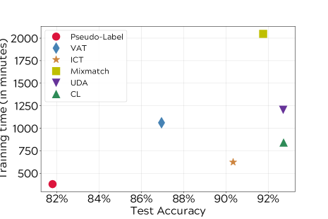
Figure 5: Comparison of time consumption and test accuracy on CIFAR-10 using 4,000 labeled samples. All the experiments were performed using Wide ResNet on an isolated virtual machine. The optimum condition between training time and accuracy is shown in the bottom right of the figure.

A.5 Pseudo-Labeled Samples

We examine some examples of pseudo-labeled images for CIFAR-10 and ImageNet, in order to provide a better intuition as to what are the typical types of examples that are being added during training. We include both some correctly and incorrectly pseudo-labeled examples, along with their prediction scores.

We show pseudo-labeled samples annotated by our method on CIFAR-10 (figure 6), and ImageNet (figure 7). We show correct and incorrect samples for 10 categories with their corresponding scores after the last iteration. We show the highest scores for each class in each column. Under the incorrectly pseudo-labeled column we also show the ground truth category for the image annotated by the model.

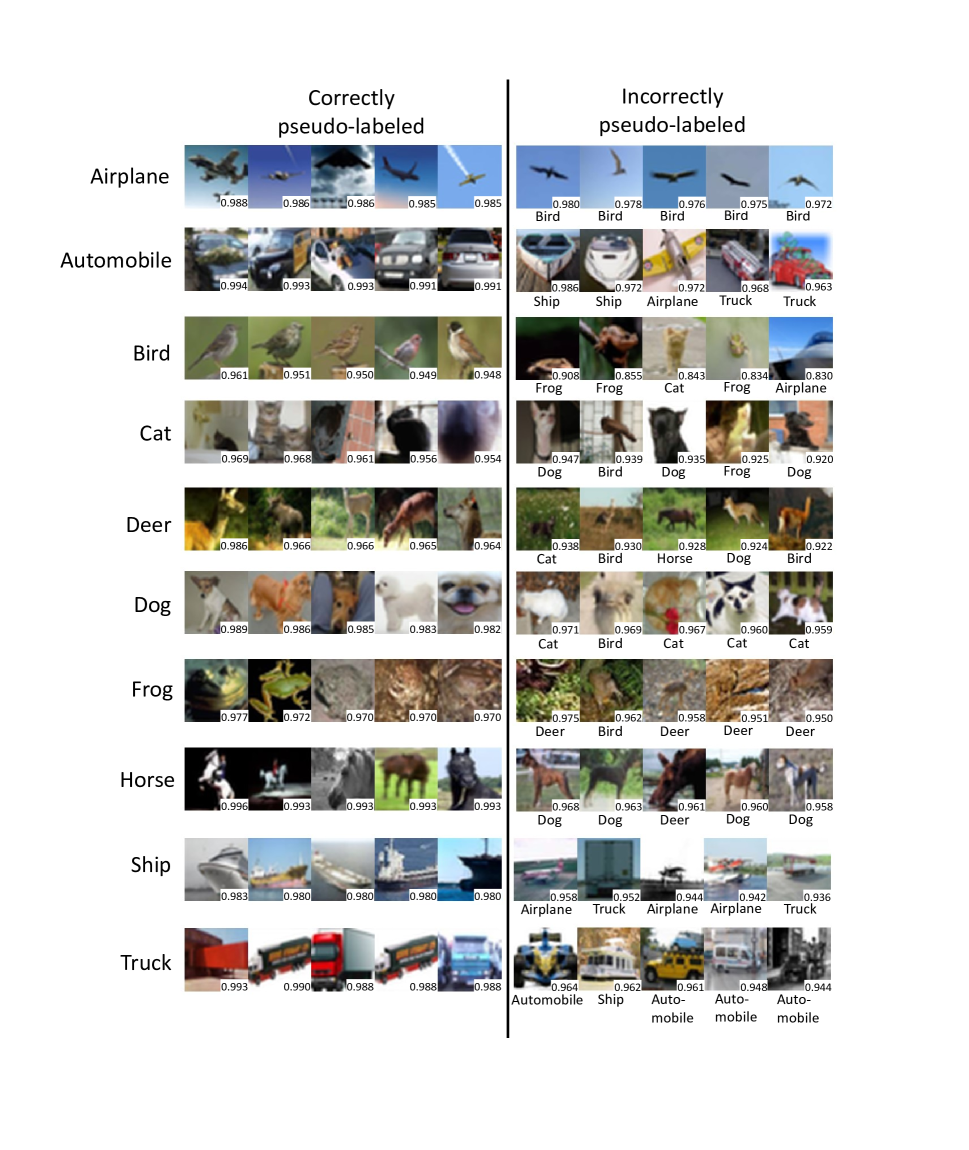
Figure 6: CIFAR-10 pseudo-labeled samples annotated by our method. We show correct and incorrect samples for the 10 categories with their corresponding scores after the last iteration.

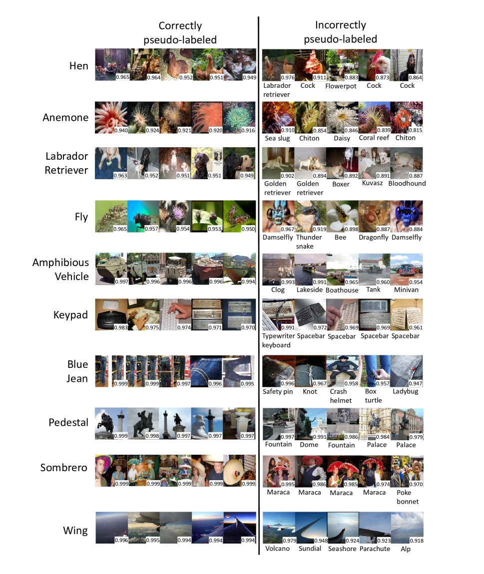
Figure 7: ImageNet pseudo-labeled samples annotated by our method. We show correct and incorrect samples for 10 chosen categories with their corresponding scores after the last iteration.

References

- Agrawala (1970) Agrawala, A. 1970. Learning with a probabilistic teacher. IEEE Transactions on Information Theory 16(4): 373–379. doi:10.1109/TIT.1970.1054472.
- Al-Behadili, Grumpe, and Wöhler (2015) Al-Behadili, H.; Grumpe, A.; and Wöhler, C. 2015. Semi-supervised Learning Using Incremental Polynomial Classifier and Extreme Value Theory. In 2015 3rd International Conference on Artificial Intelligence, Modelling and Simulation (AIMS), 332–337. doi:10.1109/AIMS.2015.60.
- Arazo et al. (2019) Arazo, E.; Ortego, D.; Albert, P.; O’Connor, N. E.; and McGuinness, K. 2019. Pseudo-Labeling and Confirmation Bias in Deep Semi-Supervised Learning.
- Bengio et al. (2009) Bengio, Y.; Louradour, J.; Collobert, R.; and Weston, J. 2009. Curriculum learning. In ICML.
- Berthelot et al. (2020) Berthelot, D.; Carlini, N.; Cubuk, E. D.; Kurakin, A.; Sohn, K.; Zhang, H.; and Raffel, C. 2020. ReMixMatch: Semi-Supervised Learning with Distribution Matching and Augmentation Anchoring. In International Conference on Learning Representations. URL https://openreview.net/forum?id=HklkeR4KPB.
- Berthelot et al. (2019) Berthelot, D.; Carlini, N.; Goodfellow, I. J.; Papernot, N.; Oliver, A.; and Raffel, C. 2019. MixMatch: A Holistic Approach to Semi-Supervised Learning. CoRR abs/1905.02249. URL http://arxiv.org/abs/1905.02249.
- Broadwater and Chellappa (2010) Broadwater, J. B.; and Chellappa, R. 2010. Adaptive Threshold Estimation via Extreme Value Theory. IEEE Transactions on Signal Processing 58(2): 490–500. ISSN 1941-0476. doi:10.1109/TSP.2009.2031285.
- Chapelle, Schlkopf, and Zien (2010) Chapelle, O.; Schlkopf, B.; and Zien, A. 2010. Semi-Supervised Learning. The MIT Press, 1st edition. ISBN 0262514125, 9780262514125.
- Chapelle and Zien (2005) Chapelle, O.; and Zien, A. 2005. Semi-Supervised Classification by Low Density Separation. In AISTATS.
- Clifton et al. (2008) Clifton, D. A.; Clifton, L. A.; Bannister, P. R.; and Tarassenko, L. 2008. Automated Novelty Detection in Industrial Systems. In Advances of Computational Intelligence in Industrial Systems.
- Clifton, Hugueny, and Tarassenko (2011) Clifton, D. A.; Hugueny, S.; and Tarassenko, L. 2011. Novelty Detection with Multivariate Extreme Value Statistics. J. Signal Process. Syst. 65(3): 371–389. ISSN 1939-8018. doi:10.1007/s11265-010-0513-6. URL http://dx.doi.org/10.1007/s11265-010-0513-6.
- Cubuk et al. (2018) Cubuk, E. D.; Zoph, B.; Mané, D.; Vasudevan, V.; and Le, Q. V. 2018. AutoAugment: Learning Augmentation Policies from Data. CoRR abs/1805.09501. URL http://arxiv.org/abs/1805.09501.
- Deng et al. (2009) Deng, J.; Dong, W.; Socher, R.; Li, L.-J.; Li, K.; and Fei-Fei, L. 2009. ImageNet: A Large-Scale Hierarchical Image Database. In CVPR09.
- Devries and Taylor (2017) Devries, T.; and Taylor, G. W. 2017. Dataset Augmentation in Feature Space. ArXiv abs/1702.05538.
- Fralick (1967) Fralick, S. 1967. Learning to recognize patterns without a teacher. IEEE Transactions on Information Theory 13(1): 57–64. doi:10.1109/TIT.1967.1053952.
- Hacohen and Weinshall (2019) Hacohen, G.; and Weinshall, D. 2019. On The Power of Curriculum Learning in Training Deep Networks. CoRR abs/1904.03626. URL http://arxiv.org/abs/1904.03626.
- Halevy, Norvig, and Pereira (2009) Halevy, A.; Norvig, P.; and Pereira, F. 2009. The Unreasonable Effectiveness of Data. Intelligent Systems, IEEE 24: 8 – 12. doi:10.1109/MIS.2009.36.
- He et al. (2015) He, K.; Zhang, X.; Ren, S.; and Sun, J. 2015. Deep Residual Learning for Image Recognition. CoRR abs/1512.03385. URL http://arxiv.org/abs/1512.03385.
- Iscen et al. (2019) Iscen, A.; Tolias, G.; Avrithis, Y.; and Chum, O. 2019. Label Propagation for Deep Semi-supervised Learning. CoRR abs/1904.04717. URL http://arxiv.org/abs/1904.04717.
- Izmailov et al. (2018) Izmailov, P.; Podoprikhin, D.; Garipov, T.; Vetrov, D. P.; and Wilson, A. G. 2018. Averaging Weights Leads to Wider Optima and Better Generalization. CoRR abs/1803.05407. URL http://arxiv.org/abs/1803.05407.
- Jackson and Schulman (2019) Jackson, J.; and Schulman, J. 2019. Semi-Supervised Learning by Label Gradient Alignment. CoRR abs/1902.02336. URL http://arxiv.org/abs/1902.02336.
- Krizhevsky (2012) Krizhevsky, A. 2012. Learning Multiple Layers of Features from Tiny Images. University of Toronto .
- Laine and Aila (2017) Laine, S.; and Aila, T. 2017. Temporal Ensembling for Semi-Supervised Learning. In 5th International Conference on Learning Representations, ICLR 2017, Toulon, France, April 24-26, 2017, Conference Track Proceedings. OpenReview.net. URL https://openreview.net/forum?id=BJ6oOfqge.
- Lee (2013) Lee, D.-H. 2013. Pseudo-Label : The Simple and Efficient Semi-Supervised Learning Method for Deep Neural Networks. ICML 2013 Workshop : Challenges in Representation Learning (WREPL) .
- Lim et al. (2019) Lim, S.; Kim, I.; Kim, T.; Kim, C.; and Kim, S. 2019. Fast AutoAugment. CoRR abs/1905.00397. URL http://arxiv.org/abs/1905.00397.
- Loshchilov and Hutter (2016) Loshchilov, I.; and Hutter, F. 2016. SGDR: Stochastic Gradient Descent with Restarts. CoRR abs/1608.03983. URL http://arxiv.org/abs/1608.03983.
- Luo et al. (2017) Luo, Y.; Zhu, J.; Li, M.; Ren, Y.; and Zhang, B. 2017. Smooth Neighbors on Teacher Graphs for Semi-supervised Learning. CoRR abs/1711.00258. URL http://arxiv.org/abs/1711.00258.
- McLachlan (1975) McLachlan, G. J. 1975. Iterative Reclassification Procedure for Constructing an Asymptotically Optimal Rule of Allocation in Discriminant Analysis. Journal of the American Statistical Association 70(350): 365–369.
- Miyato et al. (2018) Miyato, T.; ichi Maeda, S.; Koyama, M.; and Ishii, S. 2018. Virtual Adversarial Training: a Regularization Method for Supervised and Semi-supervised Learning. IEEE transactions on pattern analysis and machine intelligence .
- Netzer et al. (2011) Netzer, Y.; Wang, T.; Coates, A.; Bissacco, A.; Wu, B.; and Ng, A. Y. 2011. Reading Digits in Natural Images with Unsupervised Feature Learning. In NIPS Workshop on Deep Learning and Unsupervised Feature Learning 2011. URL http://ufldl.stanford.edu/housenumbers/nips2011–_˝housenumbers.pdf.
- Oliver et al. (2018) Oliver, A.; Odena, A.; Raffel, C. A.; Cubuk, E. D.; and Goodfellow, I. J. 2018. Realistic Evaluation of Deep Semi-Supervised Learning Algorithms. In NeurIPS.
- Perez and Wang (2017) Perez, L.; and Wang, J. 2017. The Effectiveness of Data Augmentation in Image Classification using Deep Learning. CoRR abs/1712.04621. URL http://arxiv.org/abs/1712.04621.
- Rasmus et al. (2015) Rasmus, A.; Berglund, M.; Honkala, M.; Valpola, H.; and Raiko, T. 2015. Semi-supervised Learning with Ladder Networks. In NIPS.
- Rudd et al. (2018) Rudd, E.; Jain, L. P.; Scheirer, W. J.; and Boult, T. 2018. The Extreme Value Machine. IEEE Transactions on Pattern Analysis and Machine Intelligence (T-PAMI) 40(3).
- Russakovsky et al. (2015) Russakovsky, O.; Deng, J.; Su, H.; Krause, J.; Satheesh, S.; Ma, S.; Huang, Z.; Karpathy, A.; Khosla, A.; Bernstein, M.; et al. 2015. Imagenet large scale visual recognition challenge. International journal of computer vision 115(3): 211–252.
- Sajjadi, Javanmardi, and Tasdizen (2016) Sajjadi, M.; Javanmardi, M.; and Tasdizen, T. 2016. Regularization With Stochastic Transformations and Perturbations for Deep Semi-Supervised Learning. In NIPS.
- Scudder (1965) Scudder, H. 1965. Probability of error of some adaptive pattern-recognition machines. IEEE Transactions on Information Theory 11(3): 363–371. doi:10.1109/TIT.1965.1053799.
- Shi et al. (2018) Shi, W.; Gong, Y.; Ding, C.; MaXiaoyu Tao, Z.; and Zheng, N. 2018. Transductive Semi-Supervised Deep Learning using Min-Max Features. In The European Conference on Computer Vision (ECCV).
- Shi et al. (2008) Shi, Z.; Kiefer, F.; Schneider, J.; and Govindaraju, V. 2008. Modeling biometric systems using the general pareto distribution (GPD) - art. no. 69440O. Proc SPIE doi:10.1117/12.778687.
- Shorten and Khoshgoftaar (2019) Shorten, C.; and Khoshgoftaar, T. M. 2019. A survey on Image Data Augmentation for Deep Learning. Journal of Big Data 6(1): 60. ISSN 2196-1115. doi:10.1186/s40537-019-0197-0. URL https://doi.org/10.1186/s40537-019-0197-0.
- Simard, Steinkraus, and Platt (2003) Simard, P. Y.; Steinkraus, D.; and Platt, J. C. 2003. Best practices for convolutional neural networks applied to visual document analysis. In Seventh International Conference on Document Analysis and Recognition, 2003. Proceedings., 958–963. doi:10.1109/ICDAR.2003.1227801.
- Sohn et al. (2020) Sohn, K.; Berthelot, D.; Li, C.; Zhang, Z.; Carlini, N.; Cubuk, E. D.; Kurakin, A.; Zhang, H.; and Raffel, C. 2020. FixMatch: Simplifying Semi-Supervised Learning with Consistency and Confidence. ArXiv abs/2001.07685.
- Springenberg et al. (2014) Springenberg, J. T.; Dosovitskiy, A.; Brox, T.; and Riedmiller, M. A. 2014. Striving for Simplicity: The All Convolutional Net. CoRR abs/1412.6806.
- Sun et al. (2017) Sun, C.; Shrivastava, A.; Singh, S.; and Gupta, A. 2017. Revisiting Unreasonable Effectiveness of Data in Deep Learning Era. CoRR abs/1707.02968. URL http://arxiv.org/abs/1707.02968.
- Tarvainen and Valpola (2017) Tarvainen, A.; and Valpola, H. 2017. Mean teachers are better role models: Weight-averaged consistency targets improve semi-supervised deep learning results. In ICLR.
- Verma et al. (2019) Verma, V.; Lamb, A.; Kannala, J.; Bengio, Y.; and Lopez-Paz, D. 2019. Interpolation Consistency Training for Semi-Supervised Learning. CoRR abs/1903.03825.
- Xie et al. (2019) Xie, Q.; Dai, Z.; Hovy, E. H.; Luong, M.; and Le, Q. V. 2019. Unsupervised Data Augmentation. CoRR abs/1904.12848. URL http://arxiv.org/abs/1904.12848.
- Zagoruyko and Komodakis (2016) Zagoruyko, S.; and Komodakis, N. 2016. Wide Residual Networks. CoRR abs/1605.07146. URL http://arxiv.org/abs/1605.07146.
- Zhai et al. (2019) Zhai, X.; Oliver, A.; Kolesnikov, A.; and Beyer, L. 2019. SL: Self-Supervised Semi-Supervised Learning. CoRR abs/1905.03670. URL http://arxiv.org/abs/1905.03670.
- Zhang et al. (2018) Zhang, H.; Cisse, M.; Dauphin, Y. N.; and Lopez-Paz, D. 2018. mixup: Beyond Empirical Risk Minimization. In International Conference on Learning Representations. URL https://openreview.net/forum?id=r1Ddp1-Rb.
- Zhu (2006) Zhu, X. 2006. Semi-Supervised Learning Literature Survey.