The accretion rates and mechanisms of Herbig Ae/Be stars

Abstract

This work presents a spectroscopic study of 163 Herbig Ae/Be stars. Amongst these, we present new data for 30 objects. Stellar parameters such as temperature, reddening, mass, luminosity and age are homogeneously determined. Mass accretion rates are determined from $\rm H\alpha$ emission line measurements. Our data is complemented with the X-Shooter sample from previous studies and we update results using Gaia DR2 parallaxes giving a total of 78 objects with homogeneously determined stellar parameters and mass accretion rates. In addition, mass accretion rates of an additional 85 HAeBes are determined. We confirm previous findings that the mass accretion rate increases as a function of stellar mass, and the existence of a different slope for lower and higher mass stars respectively. The mass where the slope changes is determined to be $3.98^{+1.37}_{-0.94}\,\rm M_{\sun}$. We discuss this break in the context of different modes of disk accretion for low- and high mass stars. Because of their similarities with T Tauri stars, we identify the accretion mechanism for the late-type Herbig stars with the Magnetospheric Accretion. The possibilities for the earlier-type stars are still open, we suggest the Boundary Layer accretion model may be a viable alternative. Finally, we investigated the mass accretion - age relationship. Even using the superior Gaia based data, it proved hard to select a large enough sub-sample to remove the mass dependency in this relationship. Yet, it would appear that the mass accretion does decline with age as expected from basic theoretical considerations.

1 Introduction

Herbig Ae/Be stars (HAeBes) are optically visible intermediate pre-main sequence (PMS) stars whose masses range from about 2 to 10 $\rm M_{\sun}$. These PMS stars were first identified by Herbig (1960), using three criteria: “Stars with spectral type A and B with emission lines; lie in an obscured region; and illuminate fairly bright nebulosity in its immediate vicinity”. HAeBes play an important role in understanding massive star formation, because they bridge the gap between low-mass stars whose formation is relatively well understood, and high-mass stars whose formation is still unclear. The study of their formation is not well understood as massive stars are very rare and as a consequence on average far away, and often optically invisible (Lumsden et al., 2013). A long standing problem has also been that their brightness is very high, such that radiation pressure can in principle stop accretion onto the stellar surface (Kahn, 1974). Moreover, they form very quickly and reach the main sequence before their surrounding cloud disperses (Palla & Stahler, 1993). This suggests that their evolutionary processes are very different from T Tauri stars.

The accretion onto classical T Tauri low-mass stars is magnetically controlled. The magnetic field from the star truncates material in the disc and from this point, material falls onto the star along the field line. After matter hits the photosphere, it produces X-ray radiation that is absorbed by surrounding particles. Then, these particles heat up and re-radiate at ultraviolet wavelengths, producing an UV-excess that can be observed and from which the accretion luminosity can be calculated (Bouvier et al., 2007; Hartmann et al., 2016). It was found later, that a correlation between the line luminosity and the accretion luminosity exists, allowing accretion rates of classical T Tauri stars to be determined from the UV-excess and absorption line veiling (Calvet et al., 2004; Ingleby et al., 2013).

HAeBes have similar properties as classical T Tauri stars, for instance having emission lines, UV-excess, a lower surface gravity than main-sequence stars (Hamann & Persson, 1992; Vink et al., 2005) and they are usually identified by an infrared (IR) excess from circumstellar discs (Van den Ancker et al., 2000; Meeus et al., 2001). Because their envelopes are radiative, no magnetic field is expected to be generated in HAeBe stars as this usually happens in stars by convection. Indeed, magnetic fields have rarely been detected towards them (Catala et al., 2007; Alecian et al., 2013). As a result magnetically controlled accretion is not necessarily expected to apply in the case of the most massive objects, requiring another accretion mechanism. However, how the material arrives at the stellar surface in the absence of magnetic fields is still unclear.

Several lines of evidence have indicated a difference between the lower mass Herbig Ae and higher mass Herbig Be stars. Spectropolarimetric studies suggest that Herbig Ae stars and T Tauri stars may form in the same process (Vink et al., 2005; Ababakr et al., 2017). Accretion rates of HAeBes are determined from the measurement of UV-excess (Mendigutía et al., 2011b) who have found that the relationship between the line luminosity and the accretion luminosity is similar to the classical T Tauri stars. A spectroscopic variability study suggests that a Herbig Ae star is undergoing magnetospheric accretion in the same manner as classical T Tauri stars (Schöller et al., 2016) while Mendigutía et al. (2011a) find the Herbig Be stars to have different H$\alpha$ variability properties than the Herbig Ae stars. Therefore, magnetically influenced accretion in HAeBes would still be possible. A study employing X-shooter spectra for 91 HAeBes was carried out by Fairlamb et al. (2015, 2017, hereafter F15 and F17 respectively). They determined the stellar parameters in a homogenous fashion, derived mass accretion rates from the UV-excess and found the relationship between accretion luminosity and line luminosity for 32 emission lines in the range 0.4–2.4 $\mu$m. 47 objects in their sample were taken from Thé et al. (1994, table 1), which to this date contains the strongest (candidate) members of the group. The Fairlamb papers were published before the Gaia parallaxes became available, and the distances used may need revision as these can affect parameters such as the radius, luminosity, stellar mass and mass accretion rate.

A Gaia astrometric study of 252 HAeBes was carried out by Vioque et al. (2018) hereafter V18. They presented parallaxes for all known HAeBes from the Gaia Data Release 2 (Gaia DR2) Catalogue (Gaia Collaboration et al., 2016, 2018). Also, they collected effective temperatures, optical and infrared photometry, visual extinctions, $\rm H\alpha$ equivalent widths, emission line profiles and binarities from the literature. They derived distances, luminosities, masses, ages, infrared excesses, photometric variabilities for most of their sample. This is the largest astrometric study of HAeBes to date. These Gaia DR2 parallaxes are useful for improving the stellar parameters of the previous studies.

The main aim of this paper is to determine stellar parameters and accretion rates of 30 Northern HAeBes using a homogeneous approach, extending the mostly Southern F15 sample. In parallel, the results of F15 will be updated using the distances determined from the Gaia DR2 parallaxes and a redetermined extinction towards the objects. As such, this becomes the largest homogeneous spectroscopic analysis of HAeBes to date. In addition, the accretion rates of HAeBes in the V18 study are determined for the 104 objects for which H$\alpha$ emission line equivalent widths are collected from the literature or determined from archival spectra.

The structure of this paper is as follows. Section 2 presents the spectroscopic data observation of all targets. Details of observations, instrumental setups and reduction procedures are given in this section. Section 3 and 4 detail the determination of stellar parameters and mass accretion rates. Sections 5 and 6 focus on the analysis and a discussion respectively. Section 7 provides a summary of the main conclusions of this paper.

2 Observations and Data Reduction

2.1 IDS and sample selection

The data were collected in June 2013 using the Intermediate Dispersion Spectrograph (IDS) instrument and the RED+2 CCD detector with $2048\times 4096$ pixels (pixel size 24 µm), which is attached to the Cassegrain focus of the 2.54-m Isaac Newton Telescope (INT) at the Observatorio del Roque de los Muchachos, La Palma, Spain. The observations spanned six nights between the $\rm 20^{th}$ and the $\rm 25^{th}$ June 2013. Bias frames, flat field frames, object frames and arc frames of Cu-Ar and Cu-Ne comparison lamp were taken each night to prepare for the data reduction.

In the first two nights the spectrograph was set up with a 1200 lines mm^-1 R1200B diffraction grating and a 0.9 or 1.0 arcsecond wide slit in order to obtain spectra across the Balmer discontinuity. The wavelength coverage was 3600–4600 Å, centred at 4000.5 Å. In this range the hydrogen lines of $\rm H\gamma,H\delta$, H(7-2), H(8-2), H(9-2) and H(10-2) can be analysed. This combination provides a reciprocal dispersion of 0.53 Å pixel^-1 with a spectral resolution of $\sim$ 1 Å and a resolving power of $R\sim 4000$.

For the next two nights the R1200Y grating was used to observe spectra in the visible. Its spectral range covers 5700 to 6700 Å, centred at 6050.4 Å. This range includes the He i line at 5876 Å, the [O i_λ6300] line and the $\rm H\alpha$ line at 6562 Å. This setup results in a reciprocal dispersion of 0.52 Å pixel^-1 and a resolving power of $R\sim 6500$. The final 2 nights used the R1200R grating to observe the spectral range of 8200–9200 Å, centred at 8597.2 and 8594.4 Å. This range covers the O i line at 8446 Å, all lines of the Ca ii triplet and many lines of the Paschen series. With this setup the reciprocal dispersion becomes 0.51 Å pixel^-1, giving a resolving power of $R\sim 9000$.

The sample consists of 45 targets, with 30 HAeBes, and 15 standard stars. 26 Herbig stars were chosen from the catalogue of Thé et al. (1994, table 1) and 4 from Vieira et al. (2003). About 67 per cent of HAeBes in the final sample are in the northern hemisphere. There are 7 HAeBes which are also in the sample of F15. Spectra of standard stars were observed each night for spectral comparisons. A log of the observations of the 30 HAeBes is shown in Table 1 while a log of the observations of the standard stars is presented in Table A1 (See Appendix A in the online version of this paper).

The data reduction was performed using the Image Reduction and Analysis Facility (IRAF). Standard procedures were used in order to process all frames. Generally, there are three steps of data reduction; bias subtraction, flat field division and wavelength calibration. First, many bias frames were taken and averaged to reduce some noise and the bias level was removed from the CCD data. Next, flat field division was used to remove the variations of CCD signal in each pixel. All flat frames were averaged before subtracting the bias. Then, all of the object frames were divided by the normalised flat-field frame in order to correct the pixel-to-pixel variation of the detector sensitivity. The object frame was extracted to a one-dimensional spectrum by defining the extraction aperture on the centre of the profile and subtracting the sky background. Finally, the data were wavelength calibrated. The accuracy of the wavelength calibration is measured from an RMS of the fit and is less than 10 per cent of the reciprocal dispersion ($<0.05$ Å pixel^-1). For illustration, the $\rm H\alpha$ profiles of all 30 objects are displayed in Figure B1 (See Appendix B in the online version of this paper).

3 Stellar Parameters and Mass Accretion Rate Determinations

Measurement of accretion rates requires accurate stellar parameters of the star in question. Therefore, this section aims to determine accretion rates by first determining the stellar parameters, such as the effective temperature, surface gravity, distance, radius, reddening, luminosity, mass and age. These will be determined by combining the IDS spectra, stellar model atmosphere grids, photometry from the literature, the Gaia DR2 parallaxes and stellar isochrones.

3.1 Effective temperature and surface gravity

To estimate the effective temperature of the target, a comparison of the known standard star spectra with the unknown target spectrum is performed. The list of standard stars including spectral types is shown in Table A1 (See Appendix A in the online version of this paper). The conversion from the spectral type to effective temperature can be found from Straižys & Kuriliene (1981). Then, the range of effective temperatures was explored in more detail with spectra computed from model atmospheres.

The model atmospheres used in this work are grids of BOSZ-Kurucz model atmospheres computed by Bohlin et al. (2017). The BOSZ models are calculated from ATLAS-APOGEE ATLAS9 (Mészáros et al., 2012) which came from the original ATLAS code version 9 (Kurucz, 1993). The metallicity $[\rm M/H]=0$, carbon abundance $\rm[C/H]=0$, alpha-element abundance $[\alpha/\rm H]=0$, microturbulent velocity $\xi=2.0$ km s^-1, rotational broadening velocity $v\sin i=0.0$ km s^-1, and instrumental broadening $R=5000$ are adopted. This instrumental broadening is chosen for matching the resolution of the blue spectra. The range of effective temperature $T_{\rm eff}$ is from 3500 K to 30000 K with steps of 250 K (from 3500 K to 12000 K), 500 K (from 12000 K to 20000 K) and 1000 K (from 20000 K to 30000 K). The range of surface gravity $\log(g)$ is from 0.0 dex to 5.0 dex with steps of 0.5 dex. By using linear interpolation, $\log(g)$ with steps of 0.1 dex were calculated.

The procedure to obtain the effective temperature and surface gravity in this work follows the same method by F15. The effective temperature and surface gravity determination is carried out by primarily comparing the wings of the observed hydrogen Balmer lines $\rm H\gamma$, $\rm H\delta$ and $\rm H\epsilon$ with synthetic profiles produced with solar metallicity from BOSZ models. The shapes of the hydrogen profiles are not very sensitive to metallicity (Bohlin et al., 2017) while their widths are dominated by pressure broadening, while rotation hardly affects the shapes. $\rm H\alpha$ is not used for spectral typing because it is frequently strongly in emission for HAeBes. This phenomenon can affect the shape of the wings and cause difficulty of fitting the BOSZ models to target spectra. $\rm H\beta$ is also not used for spectral typing because it appears around the edge of the blue spectrum which makes a proper characterization of $\rm H\beta$’s line profile troublesome.

In order to carry out the fitting, both the observed profiles and the synthetic profiles are normalised based on the continuum on both the blue and red side of the profile. Next, the observed wavelengths of the target profiles were corrected to the vacuum wavelength of the synthetic profile using the IRAF DOPCOR task. The effective temperature and surface gravity are obtained from the fit of the normalised synthetic spectra to the normalised observed spectra by considering continuum features and the wings of the profile above the normalised intensity of 0.8. This intensity was chosen because this part of the wings is sensitive to variation of the $\log(g)$ while the central part of the profile of a Herbig Ae/Be star can be contaminated by emission.

The width of the Balmer lines depends upon both effective temperature and surface gravity. Different combinations of $T_{\rm eff}$ and $\log(g)$, can create the same width. This degeneracy can be solved by visual inspection of absorption features in the wings and continuum either side of the lines. The final value for the effective temperature and surface gravity are the average value of the best fit for each profile ($\rm H\gamma$, $\rm H\delta$ and $\rm H\epsilon$). The uncertainties of $T_{\rm eff}$ and $\log(g)$ were chosen to be the typical difference in the values determined for the three lines respectively. If the standard error becomes zero or less than that, the step size will be adopted. An example of spectral typing by fitting the Balmer line profile of HD 141569 (black) and the BOSZ model (blue) is demonstrated in Figure 1.

Table 1: Log of observations of 30 HAeBes. Column 1 gives the object name. Columns 2 and 3 are right ascension (RA) in the units of time ($\aas@@fstack{h}$  $\aas@@fstack{m}$  $\aas@@fstack{s}$) and declination (DEC) in the units of angle ($\aas@@fstack{\circ}$  $\aas@@fstack{\prime}$  $\aas@@fstack{\prime\prime}$) respectively. Column 4 lists the observation dates. Columns 5–7 present the exposure times for each grating. The signal-to-noise ratios for each grating are given in columns 8–10. These were determined using a 20 Å wide line free spectral regions centred at the wavelength 4200, 6050 and 8800 Å for R1200B, R1200Y and R1200R grating respectively. Spectral types and photometry are listed along with references in columns 11–16.

Name	RA	DEC	Obs Date	Exposure Time (s)			SNR			Spectral Type	Photometry (mag)
	(J2000)	(J2000)	(June 2013)	R1200B	R1200Y	R1200R	B	Y	R		B	V	Rc	R	Ic
V594 Cas	00:43:18.3	+61:54:40.1	21; 23; 24	600	600	600	152	160	50	B81	11.08	10.51	10.08	-	9.5513
PDS 144	15:49:15.3	-26:00:54.8	22; 24	-	900	900	-	97	83	A5 V2	13.28	12.79	12.49	-	12.162
HD 141569	15:49:57.8	-03:55:16.3	20; 22; 24	60	60	60	302	385	194	A0 Ve3	7.23	7.13	7.08	-	7.022
HD 142666	15:56:40.0	-22:01:40.0	20; 22; 24	90; 180	90; 150	150	19	147	47	A8 Ve3	9.17	8.67	8.35	-	8.012
HD 145718	16:13:11.6	-22:29:06.7	21; 23; 25	90	180	180	30	160	74	A8 IV2	9.62	9.10	8.79	-	8.452
HD 150193	16:40:17.9	-23:53:45.2	21; 23; 24; 25	90	300	120; 300	54	258	96	A2 IVe3	9.33	8.80	8.41	-	7.9314
PDS 469	17:50:58.1	-14:16:11.8	23; 25	-	1200	1200	-	127	62	A02	13.33	12.77	12.39	-	11.952
HD 163296	17:56:21.3	-21:57:21.9	20; 23; 24; 25	60	60	60	60	270	125	A1 Vep3	6.94	6.83	6.77	-	6.7314
MWC 297	18:27:39.5	-03:49:52.1	21; 22; 24; 25	900	10; 60	1200; 600	22	16	102	B02	14.28	12.03	10.19	-	8.8014
VV Ser	18:28:47.9	+00:08:39.8	21; 23; 25	900	600	600	91	180	113	B64	12.82	11.81	11.10	-	10.3113
MWC 300	18:29:25.7	-06:04:37.3	21; 23; 25	900	600; 60	600	48	29	19	B1 Ia+[e]5	12.81	11.78	11.09	-	10.5814
AS 310	18:33:21.3	-04:58:04.8	20; 22; 24	40; 900	1200	1200	35	144	128	B1e4	13.56	12.59	11.93	-	11.2014
PDS 543	18:48:00.7	+02:54:17.1	21; 22; 24	900	1200	1200	39	153	149	B12	14.56	12.52	11.25	-	9.962
HD 179218	19:11:11.3	+15:47:15.6	21; 23; 25	60	120	120	140	311	166	A0 IVe3	7.47	7.39	7.34	-	7.292
HD 190073	20:03:02.5	+05:44:16.7	21; 23; 25	60	120	120; 300	65	205	90	A0 IVp+sh2	7.86	7.73	-	7.6615	-
V1685 Cyg	20:20:28.2	+41:21:51.6	20; 22; 24; 25	600	600; 60	600; 60	120	114	82	B2 Ve3	11.48	10.69	-	9.6316	-
LkHA 134	20:48:04.8	+43:47:25.8	20; 22; 24	600	600	600	79	192	95	B86	12.02	11.35	-	10.5616	-
HD 200775	21:01:36.9	+68:09:47.8	20; 22; 24; 25	60	60; 30	30; 60	161	192	50	B34	7.77	7.37	-	6.8416	-
LkHA 324	21:03:54.2	+50:15:10.0	21; 23; 25	900	1200	1200	52	166	123	B84	13.71	12.56	11.85	-	11.0913
HD 203024	21:16:03.0	+68:54:52.1	21; 23; 24; 25	120	180	180	56	187	65	A5 V3	9.24	9.01	9.02	-	8.6217
V645 Cyg	21:39:58.3	+50:14:20.9	21; 23; 25	900	1200	1200	20	86	152	O8.57	14.55	13.47	-	12.2816	-
V361 Cep	21:42:50.2	+66:06:35.1	20; 22; 24; 25	300	300	300	146	219	84	B44	10.65	10.21	9.89	-	9.5013
V373 Cep	21:43:06.8	+66:06:54.2	20; 22; 24	900	1200	1200	96	143	103	B88	13.22	12.33	11.7	-	11.0113
V1578 Cyg	21:52:34.1	+47:13:43.6	21; 23; 24; 25	300	300; 600	300	86	225	191	A04	10.53	10.13	-	9.6716	-
LkHA 257	21:54:18.8	+47:12:09.7	20; 22; 23; 24	900	1200	1200	54	179	129	A2e9	14.00	13.29	12.86	-	12.3917
SV Cep	22:21:33.2	+73:40:27.1	20; 22; 24	240	300	300	87	188	112	A2 IVe3	11.37	10.98	-	10.5816	-
V375 Lac	22:34:41.0	+40:40:04.5	23; 25	-	1200	1200	-	109	71	A7 Ve10	14.22	13.38	12.84	-	12.2513
HD 216629	22:53:15.6	+62:08:45.0	20; 22; 24	90	180	180	91	251	110	B3 IVe+A311	10.01	9.28	-	8.5316	-
V374 Cep	23:05:07.5	+62:15:36.5	20; 22; 24	600	450	450	121	173	138	B5 Vep12	11.14	10.28	9.71	-	9.1217
V628 Cas	23:17:25.6	+60:50:43.4	21; 23; 24; 25	900	600; 60	600	26	130	149	B0eq1	12.63	11.37	10.38	-	9.3713

References. ⁽¹⁾ Hillenbrand et al. (1992); ⁽²⁾ Vieira et al. (2003); ⁽³⁾ Mora et al. (2001); ⁽⁴⁾ Hernández et al. (2004); ⁽⁵⁾ Wolf & Stahl (1985); ⁽⁶⁾ Herbig (1958); ⁽⁷⁾ Clarke et al. (2006); ⁽⁸⁾ Dahm & Hillenbrand (2015); ⁽⁹⁾ Walker (1959); ⁽¹⁰⁾ Calvet & Cohen (1978); ⁽¹¹⁾ Skiff (2014); ⁽¹²⁾ Garrison (1970); ⁽¹³⁾ Fernandez (1995); ⁽¹⁴⁾ De Winter et al. (2001); ⁽¹⁵⁾ Oudmaijer et al. (2001); ⁽¹⁶⁾ Herbst & Shevchenko (1999); ⁽¹⁷⁾ Zacharias et al. (2012).

Figure 1: The normalised spectrum of HD 141569 fits with BOSZ model of $T_{\rm eff}=9500$ K and $\log(g)=4.2$.

For a given $T_{\rm eff}$, normally, the higher the $\log(g)$, the broader the Balmer profile. Therefore, the region of the wings of the hydrogen profile near the continuum level can be used to obtain both effective temperature and surface gravity as was mentioned earlier. Unfortunately, there is a non-linear relationship between the surface gravity and width of the Balmer profile for objects that have $T_{\rm eff}<8000$ K. For this reason, a spectroscopic $\log(g)$ can not be determined and the surface gravity is calculated instead using the stellar mass and radius (see later). For 3 objects (PDS 144S, PDS 469 and V375 Lac) no near UV blue spectra were taken during the observations. Fortunately, a FEROS spectrum of PDS 469 was found in the ESO Science Archive Facility and was used to determine temperature and surface gravity. In the case of PDS 144S and V375 Lac, visible spectra including $\rm H\alpha$ profiles in combination with spectral types from the literature were investigated in order to adopt their effective temperatures.

7 objects show extremely strong emission lines. These strong emissions have an influence on the wings on even the whole Balmer profiles. Both $T_{\rm eff}$ and $\log(g)$ could therefore not be determined by this method. Instead, for these objects, estimated temperatures from the literature are adopted. The stars for which this process is performed on are noted in the last column of Table 2.

There are 7 objects in this work that overlap with F15. The difference in temperatures of these objects is on average 180 K, which is smaller than the step-size used by both studies. Figure 2 compares the effective temperature derived in this work (Table 2) with estimated values from the literature. The good correlation would suggest that our method is reliable, the fact that it is applied to the entire sample ensures a homogeneous study.

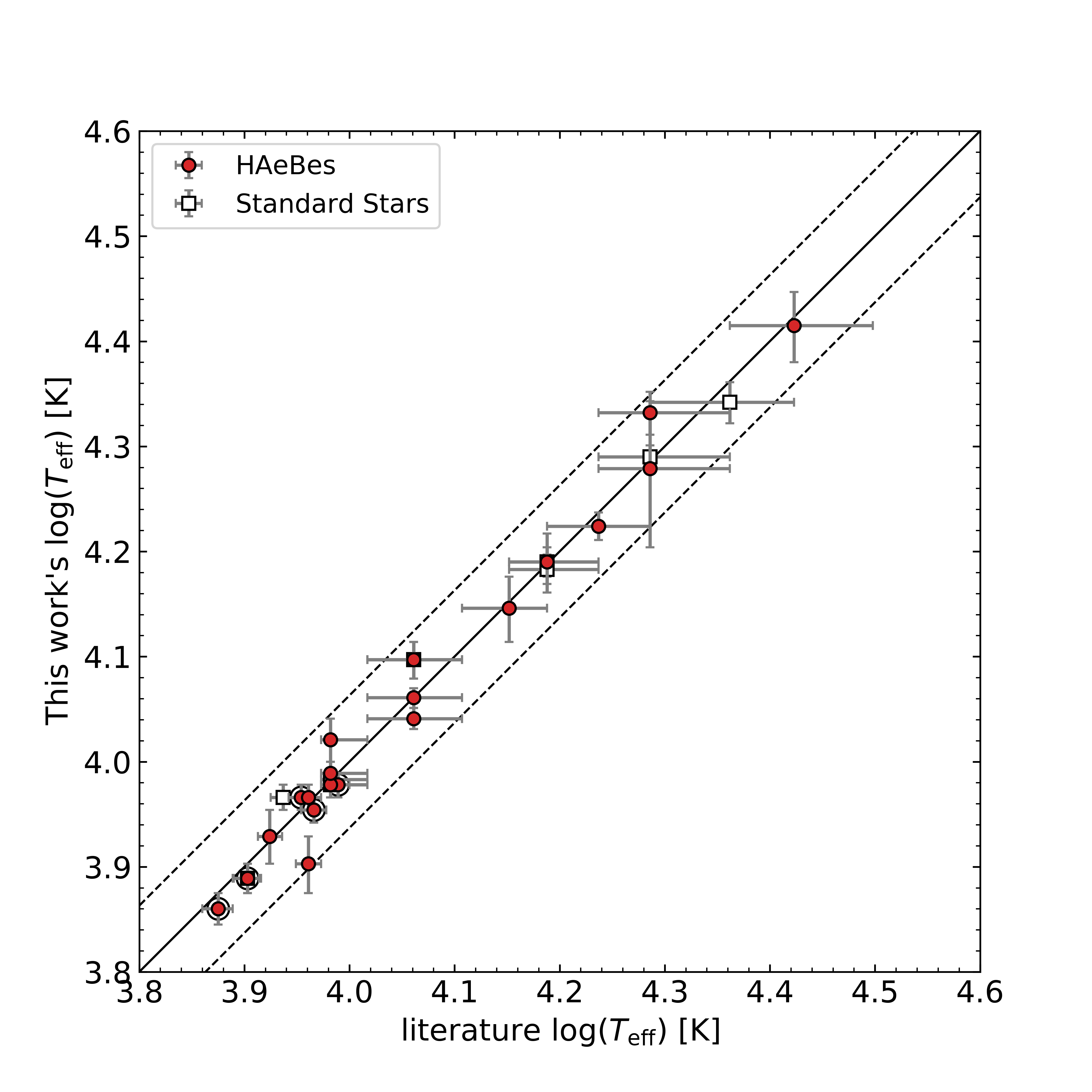
Figure 2: The effective temperature derived in this work compared to temperatures derived from spectral types in the literature listed in Table 1 and Table A1. The spectral type was converted to temperature using the values provided in Straižys & Kuriliene (1981), and an uncertainty of a subclass of spectral type was assigned for the temperature. HAeBes and standard stars are denoted in circle and square respectively. Circles with larger circle around them indicate the objects that temperature from Fairlamb et al. (2015) is used. The standard deviation ($\sigma$) between both $\log(T_{\rm eff})$ is only 0.02. The solid line is the expected line of correlation and the dashed lines are $3\,\sigma$ deviation from the solid line.

3.2 Visual extinction, distance and radius

The second step is to use the synthetic BOSZ spectral energy distribution and previous photometry results to determine the visual extinction or reddening ($A_{V}$) by fitting the synthetic surface flux density to observed photometry. In the case of zero extinction or for extinction corrected photometry, the flux density $f$ of the BOSZ model and the observed fluxes differ by the ratio of distance to the star and its radius ($D/R_{*}$). The spectral energy distribution grid of the BOSZ models are set up for the effective temperatures from the previous step with a range of scaling factors $D/R_{*}$. The value of $\log(g)$ does not have a significant effect on the spectral energy distribution shape. Therefore, $\log(g)=4.0$ was adopted at this stage.

The observed photometry is dereddened using the extinction values $A_{\lambda}/A_{V}$ from Cardelli et al. (1989) with the standard ratio of total to selective extinction parameter $R_{V}=3.1$ and zero-magnitude fluxes from Bessell (1979). By varying $A_{V}$ in steps of 0.01 magnitude, the best fit of the photometry and BOSZ models will then yield the best fitting reddening values. Only the BVRI magnitudes are used, as the U-band and JHKLM photometry are often affected by the Balmer continuum excess and IR-excess emission respectively, i.e. they can not automatically be used in the fitting. All of the observed BVR_cI_c or BVR photometry from the literature are shown in Table 1. For 3 objects (HD 203024, LkHA 257 and V374 Cep) their Sloan photometry needed to be converted to Johnson-Cousins photometry. This was done using the transformation equations provided by Smith et al. (2002). The uncertainties in the resulting $A_{V}$ and $D/R_{*}$ are assigned to be at values that resulted twice of the minimum chi-squared value. Figure 3 demonstrates an example of photometry fitting.

Figure 3: The synthetic spectral energy distribution BOSZ model (black line) is fitted to the dereddened photometry (red point) of HD 141569. The observed BVR_cI_c photometry of HD 141569 were taken from Vieira et al. (2003). A synthetic spectral energy distribution BOSZ model with $T_{\rm eff}=9500$ K and $\log(g)=4.0$ is fitted to the dereddened photometry. This provides the reddening $A_{V}=0.38^{+0.02}_{-0.03}$ mag and the scaling factor $D/R_{*}=63.7^{+1.1}_{-0.7}$ pc/$\rm R_{\sun}$.

The scaling factor $D/R_{*}$ allows us to calculate stellar radius $R_{*}$, provided the stellar distance $D$ is known. The Gaia DR2 catalogue provides astrometric parameters, such as positions, proper motions and parallaxes for more than 1.3 billion targets including most of the known HAeBes. The distances to most of our targets were determined by V18 using Gaia DR2 parallaxes. Re-normalised unit weight error (RUWE) is used to select sources with good astrometry. We adopted RUWE $<1.4$ as a criterion for good parallaxes (see Gaia Data Release 2 document). 7 stars have low quality parallaxes, and for 2 stars no parallaxes are presented in the Gaia archive. These are noted in the final column of Table 2. In total, stellar radii could be determined for 26 out of the 30 targets.

3.3 Stellar luminosity, mass and age

Using the stellar radius $R_{*}$ and the effective temperature $T_{\rm eff}$, the luminosity $L_{*}$ can be determined from the Stefan-Boltzmann law. The next step is to estimate the mass and age of the HAeBes using isochrones. Stellar isochrones of Marigo et al. (2017) from 0.01 to 100 Myr are used in order to extract a mass and an age of the target from the luminosity-temperature Hertzsprung-Russell diagram. A metallicity $Z=0.01$ and helium mass fraction $Y=0.267$ are chosen, because these values are close to solar values.

After each star is placed on the HR diagram, the two closest points on an isochrone are used to obtain the mass of the star by interpolating between those points. Uncertainties of mass and age are derived from the error bars of the effective temperature $T_{\rm eff}$ and the luminosity $L_{*}$ on the HR diagram. All determined parameters of all targets are presented in Table 2. The positions of the 21 HAeBes on the HR diagram are represented with red symbols in Figure 4 As mentioned above, the 9 targets that are not included in the plot have low quality parallaxes or do not have parallaxes at all. Since the 3 objects (HD 142666, HD 145718 and SV Cep) have had $T_{\rm eff}<8000$ K, their surface gravity cannot be determined from fitting the spectra with stellar atmospheric models. Instead, their surface gravities were calculated from the stellar mass and radius derived from the parallexes instead. These are also noted in the $\log(g)$ column of Table 2.

Table 2: Determined stellar parameters. Columns 2–9 are effective temperature, surface gravity, visual extinction, distance, radius, luminosity, mass and age respectively. Distance $D$ in column 5 is obtained from Vioque et al. (2018). This table is available in electronic form at https://cdsarc.unistra.fr/viz-bin/cat/J/MNRAS/493/234.

Name	$T_{\rm eff}$	$\log(g)$	$A_{V}$	$D$	$R_{*}$	$\log(L_{*})$	$M_{*}$	Age
	(K)	[cm s-2]	(mag)	(pc)	($\rm R_{\sun}$)	[$\rm L_{\sun}$]	($\rm M_{\sun}$)	(Myr)
V594 Cas	$11500^{+250}_{-250}$	$3.70^{+0.10}_{-0.10}$	$2.27^{+0.18}_{-0.23}$	$569^{+16}_{-14}$	$3.86^{+0.52}_{-0.53}$	$2.37^{+0.15}_{-0.17}$	$3.51^{+0.45}_{-0.42}$	$1.29^{+0.53}_{-0.38}$
PDS 144S	$7750^{+500}_{-500}$ a	$4.00^{+0.30}_{-0.30}$	$1.02^{+0.07}_{-0.07}$	-d	-	-	-	-
HD 141569	$9500^{+250}_{-250}$	$4.20^{+0.10}_{-0.10}$	$0.38^{+0.02}_{-0.03}$	$110.63^{+0.91}_{-0.88}$	$1.74^{+0.03}_{-0.04}$	$1.34^{+0.06}_{-0.07}$	$2.06^{+0.02}_{-0.15}$	$5.89^{+1.87}_{-0.64}$
HD 142666	$7250^{+250}_{-250}$	$4.00^{+0.10}_{-0.10}$ c	$0.82^{+0.07}_{-0.08}$	$148.3^{+2}_{-1.9}$	$2.21^{+0.11}_{-0.12}$	$1.08^{+0.10}_{-0.11}$	$1.64^{+0.12}_{-0.11}$	$7.76^{+1.79}_{-1.30}$
HD 145718	$7750^{+250}_{-250}$	$4.20^{+0.10}_{-0.10}$ c	$1.10^{+0.06}_{-0.06}$	$152.5^{+3.2}_{-3}$	$1.85^{+0.10}_{-0.10}$	$1.05^{+0.10}_{-0.10}$	$1.62^{+0.07}_{-0.03}$	$8.71^{+0.84}_{-1.12}$
HD 150193	$9250^{+250}_{-250}$	$4.10^{+0.10}_{-0.10}$	$1.88^{+0.16}_{-0.20}$	$150.8^{+2.7}_{-2.5}$	$2.34^{+0.26}_{-0.27}$	$1.56^{+0.14}_{-0.15}$	$2.12^{+0.21}_{-0.12}$	$4.57^{+0.93}_{-1.02}$
PDS 469	$9500^{+750}_{-750}$ a	$3.80^{+0.30}_{-0.30}$	$1.94^{+0.12}_{-0.13}$	-d	-	-	-	-
HD 163296	$9000^{+250}_{-250}$	$4.10^{+0.10}_{-0.10}$	$0.29^{+0.01}_{-0.02}$	$101.5^{+2}_{-1.9}$	$1.87^{+0.05}_{-0.05}$	$1.31^{+0.07}_{-0.07}$	$1.95^{+0.07}_{-0.07}$	$6.03^{+0.28}_{-0.27}$
MWC 297	$24000^{+2000}_{-2000}$ b	$4.00^{+0.10}_{-0.10}$	$7.87^{+0.41}_{-0.64}$	$375^{+22}_{-18}$	$9.28^{+3.12}_{-3.04}$	$4.41^{+0.39}_{-0.50}$	$14.53^{+6.11}_{-4.84}$	$0.04^{+0.07}_{-0.02}$
VV Ser	$14000^{+1000}_{-1000}$	$4.30^{+0.30}_{-0.30}$	$3.74^{+0.22}_{-0.27}$	-d	-	-	-	-
MWC 300	$23000^{+2000}_{-2000}$ b	$3.00^{+0.20}_{-0.20}$	$3.85^{+0.21}_{-0.28}$	$1400^{+250}_{-160}$	$6.02^{+1.96}_{-1.44}$	$3.96^{+0.39}_{-0.39}$	$10.09^{+3.76}_{-1.89}$	$0.09^{+0.09}_{-0.05}$
AS 310	$26000^{+2000}_{-2000}$	$4.40^{+0.35}_{-0.35}$	$3.86^{+0.20}_{-0.24}$	$2110^{+350}_{-240}$	$5.70^{+1.71}_{-1.27}$	$4.13^{+0.36}_{-0.36}$	$11.60^{+3.92}_{-2.18}$	$0.07^{+0.08}_{-0.04}$
PDS 543	$28500^{+2500}_{-2500}$ b	$4.00^{+0.10}_{-0.10}$	$7.11^{+0.28}_{-0.40}$	$1410^{+240}_{-160}$	$16.24^{+5.99}_{-4.57}$	$5.19^{+0.42}_{-0.45}$	$30.02^{+18.28}_{-10.85}$	$0.01^{+0.01}_{-0.01}$
HD 179218	$9500^{+250}_{-250}$	$3.95^{+0.10}_{-0.10}$	$0.33^{+0.02}_{-0.02}$	$266^{+5.6}_{-5.2}$	$3.62^{+0.12}_{-0.11}$	$1.98^{+0.07}_{-0.07}$	$2.86^{+0.16}_{-0.20}$	$2.04^{+0.47}_{-0.26}$
HD 190073	$9750^{+250}_{-250}$	$3.50^{+0.10}_{-0.10}$	$0.20^{+0.04}_{-0.04}$	$870^{+100}_{-70}$	$9.23^{+1.28}_{-0.94}$	$2.84^{+0.16}_{-0.14}$	$5.62^{+0.78}_{-0.65}$	$0.28^{+0.14}_{-0.10}$
V1685 Cyg	$23000^{+4000}_{-4000}$ b	$4.06^{+0.10}_{-0.10}$	$3.33^{+0.34}_{-0.51}$	$910^{+46}_{-39}$	$5.48^{+1.51}_{-1.51}$	$3.88^{+0.49}_{-0.61}$	$9.53^{+4.57}_{-2.55}$	$0.11^{+0.27}_{-0.07}$
LkHA 134	$11000^{+250}_{-250}$	$4.00^{+0.10}_{-0.10}$	$2.44^{+0.19}_{-0.24}$	$843^{+36}_{-31}$	$4.53^{+0.71}_{-0.70}$	$2.43^{+0.17}_{-0.19}$	$3.77^{+0.56}_{-0.56}$	$1.02^{+0.60}_{-0.34}$
HD 200775	$19000^{+3000}_{-3000}$	$4.27^{+0.25}_{-0.25}$	$1.85^{+0.15}_{-0.17}$	-d	-	-	-	-
LkHA 324	$12500^{+500}_{-500}$	$4.00^{+0.10}_{-0.10}$	$3.94^{+0.14}_{-0.16}$	$605^{+16}_{-14}$	$3.15^{+0.34}_{-0.33}$	$2.34^{+0.16}_{-0.17}$	$3.36^{+0.41}_{-0.30}$	$1.51^{+0.49}_{-0.41}$
HD 203024	$8500^{+500}_{-500}$	$3.83^{+0.29}_{-0.29}$	$0.52^{+0.24}_{-0.31}$	-e	-	-	-	-
V645 Cyg	$30000^{+7000}_{-7000}$ b	$3.75^{+0.35}_{-0.35}$	$4.21^{+0.29}_{-0.40}$	-d	-	-	-	-
V361 Cep	$16750^{+500}_{-500}$	$4.00^{+0.10}_{-0.10}$	$1.97^{+0.14}_{-0.15}$	$893^{+35}_{-31}$	$4.34^{+0.52}_{-0.48}$	$3.12^{+0.15}_{-0.15}$	$5.56^{+0.65}_{-0.57}$	$0.40^{+0.16}_{-0.11}$
V373 Cep	$11500^{+1250}_{-1250}$ b	$3.50^{+0.50}_{-0.50}$	$3.24^{+0.20}_{-0.23}$	-d	-	-	-	-
V1578 Cyg	$10500^{+500}_{-500}$	$3.80^{+0.20}_{-0.20}$	$1.46^{+0.08}_{-0.08}$	$773^{+30}_{-27}$	$4.77^{+0.41}_{-0.37}$	$2.39^{+0.15}_{-0.15}$	$3.74^{+0.45}_{-0.41}$	$1.02^{+0.39}_{-0.28}$
LkHA 257	$9250^{+250}_{-250}$	$4.05^{+0.10}_{-0.10}$	$2.28^{+0.07}_{-0.08}$	$794^{+18}_{-16}$	$1.84^{+0.11}_{-0.11}$	$1.35^{+0.10}_{-0.10}$	$1.98^{+0.06}_{-0.04}$	$5.76^{+1.32}_{-0.51}$
SV Cep	$8000^{+500}_{-500}$	$4.37^{+0.11}_{-0.11}$ c	$0.78^{+0.04}_{-0.05}$	$344.3^{+4}_{-3.8}$	$1.48^{+0.05}_{-0.06}$	$0.91^{+0.14}_{-0.15}$	$1.63^{+0.04}_{-0.14}$	$11.00^{+10.40}_{-2.49}$
V375 Lac	$8000^{+750}_{-750}$ a	$4.30^{+0.10}_{-0.10}$	$2.31^{+0.14}_{-0.16}$	-e	-	-	-	-
HD 216629	$21500^{+1000}_{-1000}$	$4.00^{+0.10}_{-0.10}$	$2.86^{+0.13}_{-0.15}$	$805^{+31}_{-27}$	$7.59^{+0.94}_{-0.83}$	$4.04^{+0.18}_{-0.18}$	$10.83^{+1.71}_{-1.54}$	$0.07^{+0.04}_{-0.02}$
V374 Cep	$15500^{+1000}_{-1000}$	$3.50^{+0.10}_{-0.10}$	$3.20^{+0.15}_{-0.18}$	$872^{+40}_{-35}$	$7.72^{+1.05}_{-0.98}$	$3.49^{+0.22}_{-0.23}$	$7.50^{+1.46}_{-1.28}$	$0.16^{+0.12}_{-0.06}$
V628 Cas	$31000^{+5000}_{-5000}$ b	$4.00^{+0.10}_{-0.10}$	$5.05^{+0.36}_{-0.55}$	-d	-	-	-	-

Notes. ^(a) Stars for which NUV-B spectra were not obtained. ^(b) Stars which display extremely strong emission lines. ^(c) Stars for which parallactic $\log(g)$ is used. ^(d) Stars which have low quality parallaxes in the Gaia DR2 Catalogue (see the text for discussion). ^(e) Stars which do not have parallaxes in the Gaia DR2 Catalogue.

3.4 Extending the sample with HAeBes in the southern hemisphere

The original driver for the INT observations presented here was to extend the spectroscopic analysis of the, mostly southern, sample of F15 to the northern hemisphere. However, F15 determined spectroscopic distances using their spectral derived values of the surface gravity or literature values for the distances to their 91 HAeBes. The availability of Gaia-derived distances warrants a re-determination of the stellar parameters. To this end we use the distances from the Gaia DR2 parallax (V18). In parallel, we re-assessed the extinction values using the same photometric bands BVR_cI_c as above to ensure consistency in the determination of the extinction. Most of the photometry used for the photometry fitting can be found in Fairlamb et al. (2015, table A1). We collated Sloan photometry from Zacharias et al. (2012) for 3 objects (HD 290500, HT CMa and HD 142527) and one object, HD 95881, from APASS DR10 and converted these to the Johnson-Cousins system. Moreover, we also used the brightest V-band magnitude of Johnson BVR photometry for 2 objects, HD 250550 and KK Oph, and Johnson BVRI photometry for Z CMa from Herbst & Shevchenko (1999). The redetermined stellar parameters for the 91 HAeBes from F15 are listed in Table C1 (See Appendix C in the online version of this paper). For the sample as a whole, the luminosities resulting from the revised distances and extinctions are on average similar to the original F15 values, however the contribution to the scatter around the mean differences is dominated by the new distances. We thus conclude that the improvement in distance values dominates that of the extinction when arriving at the final luminosities.

We now have the largest spectroscopic sample of HAeBes and the homogeneously determined stellar parameters including mass accretion rates, which will be determined in the next section. 7 targets in F15’s sample which are also in this work’s sample were left out, leaving 84 HAeBes in their sample. Unfortunately, 22 out of the 84 objects (not including PDS 144S) have low quality or do not have a Gaia DR2 parallax. These objects cannot be placed on the HR diagram at this stage. The final sample contains 83 Herbig Ae/Be objects. Figure 4 demonstrates all these HAeBes ($21+62$) placed in the HR diagram. Many targets are gathered around $2\,\rm M_{\sun}$ and few targets are located at high-mass tracks. This can be understood by the initial mass function IMF (Salpeter, 1955). Low-mass stars are more common than high-mass stars. Moreover, low-mass stars evolve slower across the HR diagram.

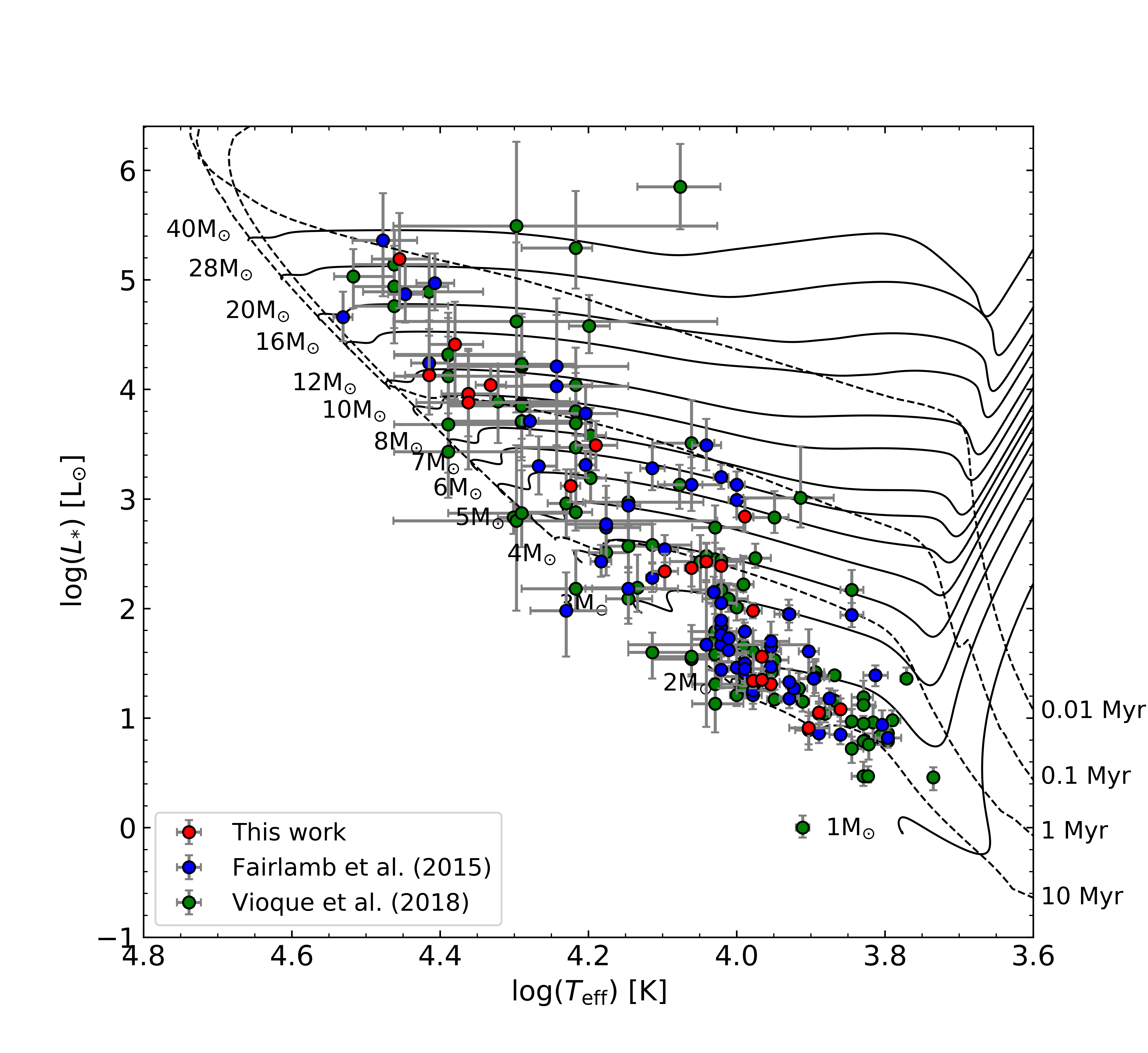
Figure 4: The placement of all 184 HAeBes in the HR diagram. The red circles are this work sample of 21 HAeBes, whereas 62 HAeBes in the sample of Fairlamb et al. (2015) are denoted as the blue circles and 101 HAeBes in Vioque et al. (2018) are shown as the green circles. All of these objects satisfy the condition RUWE $<1.4$. The PMS tracks with initial mass from 1 to 40 $\rm M_{\sun}$ (Bressan et al., 2012; Tang et al., 2014) are plotted as solid lines and isochrones of 0.01, 0.1, 1 and 10 Myr (Marigo et al., 2017) are plotted as dashed lines.

3.5 Combining with additional HAeBes with Gaia DR2 data from V18

In order to expand the sample further, the rest of 144/252 objects in the sample of V18 were investigated. There are 101 objects which satisfy the condition RUWE $<1.4$. They are also included in Figure 4. H$\alpha$ equivalent widths are provided for most objects in Vioque et al. (2018, their table 1 and table 2) with references. Spectra for 14 objects without H$\alpha$ data in the V18 sample were found in the ESO Science Archive Facility. These were downloaded and their H$\alpha$ EWs were measured. The stellar radii and surface gravities were calculated using the temperatures, luminosities and masses provided in V18. The intrinsic equivalent widths were measured from BOSZ models for the temperature provided in Vioque et al. (2018, table 1 and table 2) and the calculated surface gravity. This will enable us to compute mass accretion rates for a further 85 objects below. Table D1 presents all of the emission lines measurements and determined accretion rates of the V18 sample (See Appendix D in the online version of this paper).

4 Accretion rate determination

We now will determine the mass accretion rates of the combined sample of Herbig Ae/Be stars. The underlying assumption of the methodology is that the stars accrete material according to the MA paradigm, which, as demonstrated by Muzerolle et al. (2004), can explain the observed excess fluxes in Herbig Ae/Be stars. The infalling material shocking the photosphere gives rise to UV-excess emission, whose measurement can be converted into an accretion luminosity. Knowledge of the stellar parameters can then return a value of the mass accretion rate.

F15 derived the accretion rates for their sample from the UV excess following the methodology of Muzerolle et al. (2004) and extending the work of Mendigutía et al. (2011b). Unfortunately, as mentioned before, our current observational set-up did not allow for such accurate measurements. However, as for example pointed out by Mendigutía et al. (2011b), the accretion luminosity correlates with the line strengths of various types of emission lines. They will therefore also correlate with the mass accretion rate (see also Fairlamb et al. 2017). As such, the line strengths do provide an observationally cheap manner to derive the accretion rate of an object without having to resort to the rather delicate and time-consuming process of measuring the UV excess. We should note that despite this, it is not clear whether the observed correlation is intrinsically due to accretion or some other effect (Mendigutía et al., 2015a).

We have chosen the H$\alpha$ line for the accretion luminosity determination, as these lines are strongest lines present in the spectra. To arrive at a measurement of the total line emission, we need to take account of the fact that the underlying line absorption is filled in with emission. Therefore, the intrinsic absorption equivalent width $EW_{\rm int}$ needs to be subtracted from the observed equivalent width $EW_{\rm obs}$. The intrinsic EW is measured from the synthetic spectra corresponding to the effective temperature and surface gravity determined earlier.

The line luminosity $L_{\rm line}$ was calculated using the unreddened stellar flux at the wavelength of H$\alpha$ and distance to the star. The relationship between accretion luminosity and line luminosity goes as (cf. e.g. Mendigutía et al. 2011b).

$$\log\left(\frac{L_{\rm acc}}{\rm L_{\sun}}\right)=A+B\times\log\left(\frac{L_{\rm line}}{\rm L_{\sun}}\right),$$ (1)

where $A$ and $B$ are constants corresponding to the intercept and the gradient of the relation between $\log(L_{\rm acc}/\rm L_{\sun})$ and $\log(L_{\rm line}/\rm L_{\sun})$ respectively. This relationship has, most recently, been determined for 32 accretion diagnostic emission lines by F17. For the case of $\rm H\alpha$, the constants are $A=2.09\pm 0.06$ and $B=1.00\pm 0.05$. The mass accretion rate is then determined from the accretion luminosity, stellar radius and stellar mass by Equation 2.

$$\dot{M}_{\rm acc}=\frac{L_{\rm acc}R_{*}}{GM_{*}}$$ (2)

Table 3 summarises the EW measurements for the $\rm H\alpha$ line and mass accretion rates in all HAeBes.

The final set of 78 mass accretion rates (21+57) based on the INT and X-Shooter data is the largest, and arguably the best such collection to date as they were determined in a homogeneous and consistent manner. To arrive at the largest sample possible however, we expand the sample using data provided in the comprehensive study by V18. Adding 85 objects from V18 results in a large sample of 163 Herbig Ae/Be stars with mass accretion rates

5 Analysis

We have obtained new spectroscopic data of 30 northern Herbig Ae/Be stars which are used to determine their stellar parameters, extinction and H$\alpha$ emission line fluxes. Combined with Gaia DR2 parallaxes, this led to the determination of the mass accretion rates for 21 of these objects. This dataset complements the large southern sample of F15, for which we re-determined stellar parameters using the Gaia parallaxes and extinctions in the same manner as for the northern sample. This full sample contains 78 objects with homogeneously determined values. To this we add 85 objects from the V18 study for which literature values have been adapted and new H$\alpha$ line measurements have been added using data from archives. This led to a total of 163 objects for which we have stellar parameters, distances, H$\alpha$ emission line fluxes and mass accretion rates derived from these using the MA paradigm available. In the following we will investigate the dependence of the MA-derived accretion rate on stellar mass, and find that there is a break in properties around 4M_⊙.

5.1 Accretion luminosity as a function of stellar luminosity

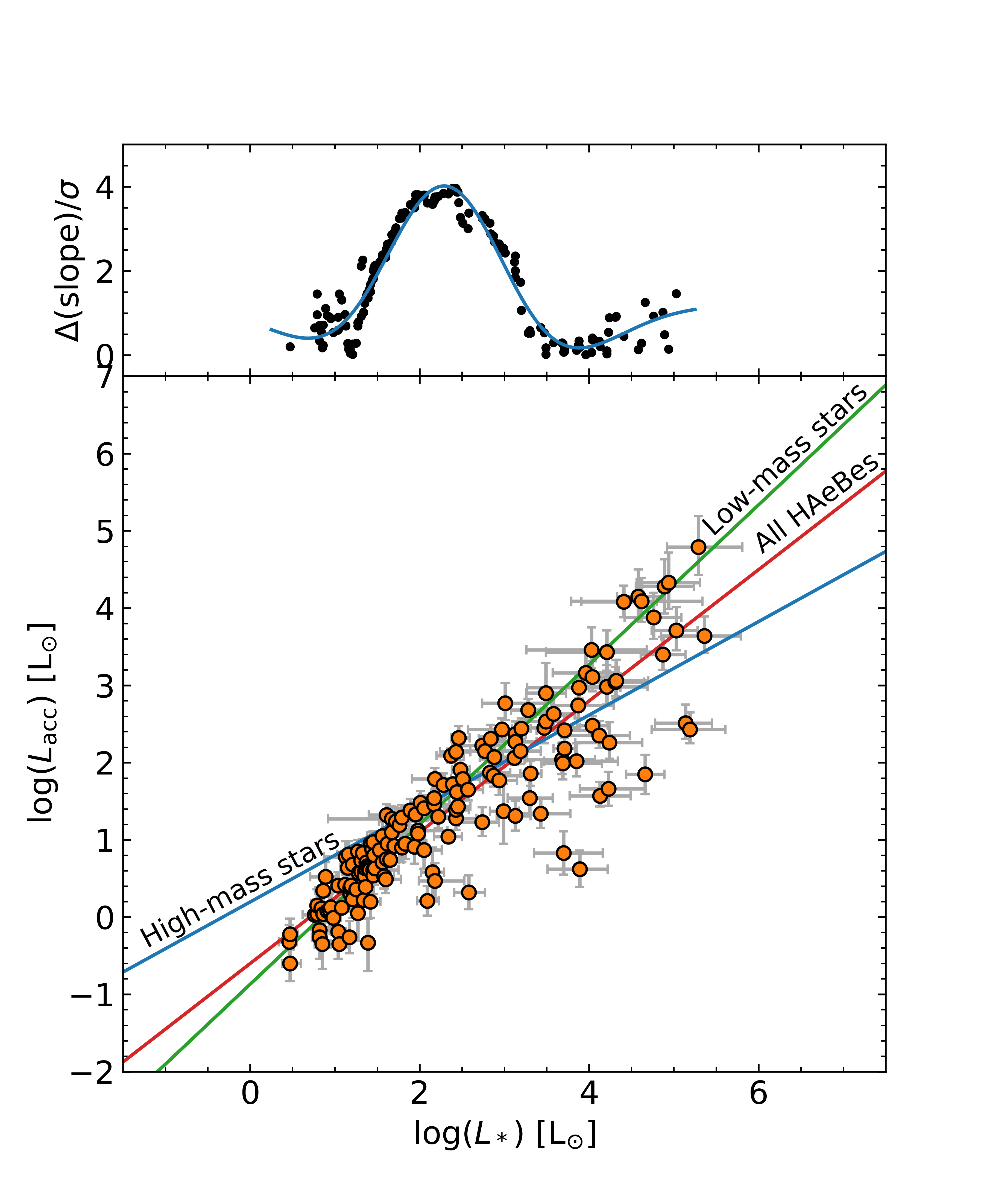
Figure 6: The logarithmic accretion luminosities versus stellar luminosities for the full, 163 stars, sample. Also shown are linear fits to the full sample and to the low- and high-mass stars respectively. As can be seen in the top panel, the difference in slopes between the low- and high-mass objects is most significant at at $L_{*}>194\,\rm L_{\sun}$ (see text for details). The gradients of best fits for the whole sample, low-mass and high-mass HAeBes are $0.85\pm 0.03$, $1.03\pm 0.08$ and $0.60\pm 0.08$ respectively.

Before addressing the mass accretion rate, let us first discuss the accretion luminosity, as that is less dependent on the stellar parameters. In Figure 6 we show the accretion luminosity versus the stellar luminosity for the entire sample. The accretion luminosity increases monotonically with stellar luminosity, which confirms earlier reports (F15, Mendigutía et al. 2011b). However, the sample under consideration is much larger than previously.

It would appear that the slope decreases, while the scatter in the relationship increases, with mass. To investigate whether there is a significant difference in accretion luminosities between high- and low mass objects, and if so, to determine the mass where there is a turn-over, we split the data into a low mass and a high mass sample, with a varying turnover mass. We then fitted a straight line to the data from the lowest mass to this intermediate mass, and a straight line from the intermediate mass to the largest mass. The intermediate mass was varied from the second smallest to the second largest mass.

This resulted in values of the slopes and their statistical uncertainty for a range of masses. When taking the difference in slopes and expressing this in terms of the respective uncertainties in the fit, we arrive at a statistical assessment whether the low- and high mass samples have a different slope. This approach takes into account the issue that the absolute value of the difference-in-slopes may not be a reliable indicator of the turn-over point. This is because each slope can vary depending on both the number and spread of data points used. For example, at both the high and low mass ends, the slopes will have a large uncertainty simply because of small number statistics.

We quantify the difference in slopes by combining the uncertainties on both low and high mass gradients, $\sigma$, and compare this to the difference in slopes, $\Delta$(slope). This is shown in the top panel of Figure 6. The $\Delta$(slope) reaches its maximum significance of 4$\sigma$ for a luminosity of 194 L_⊙, which was determined by a triple-Gaussian fit to the curve. For the lower mass HAeBes, the linear best fit provides the empirical calibration of $\log\left(\frac{L_{\rm acc}}{\rm L_{\sun}}\right)=(-0.87\pm 0.11)+(1.03\pm 0.08)\times\log\left(\frac{L_{*}}{\rm L_{\sun}}\right)$. This is in agreement with the best fit for low-mass stars in the work of Mendigutía et al. (2011b) ($L_{\rm acc}\propto L^{1.2}_{*}$). For the higher mass HAeBes, the best fit provides the expression of $\log\left(\frac{L_{\rm acc}}{\rm L_{\sun}}\right)=(0.19\pm 0.27)+(0.60\pm 0.08)\times\log\left(\frac{L_{*}}{\rm L_{\sun}}\right)$.

5.2 Mass accretion rate as a function of stellar mass

One of the main questions regarding the formation of massive stars is at which mass the mass accretion mechanism changes from magnetically controlled accretion to another mechanism, which could be direct accretion from the disk onto the star. Above we saw that there is a difference in the accretion luminosity to stellar luminosity relationships for different masses. So, we now move to look at the mass accretion rates and investigate various subsamples individually.

Table 3: The equivalent width measurements and accretion rates. Column 2 provides the $\rm H\alpha$ emission line profile classification scheme according to Reipurth et al. (1996): single-peaked (I); double-peaked and the secondary peak rises above half strength of the primary peak (II); double-peaked and the secondary peak rises below half strength of the primary peak (III), when the secondary peak is located blueward or redward of the primary peak, class II and III are label with B or R respectively; regular P-Cygni profile (IV B); and inverse P-Cygni profile (IV R). The classifications are based on the emission lines in Figure B1 corrected for absorption. Columns 3–10 present observed equivalent width, intrinsic equivalent width, corrected equivalent width, continuum flux density at central wavelength of the $\rm H\alpha$ profile, line flux, line luminosity, accretion luminosity and mass accretion rate respectively. This table is available in electronic form at https://cdsarc.unistra.fr/viz-bin/cat/J/MNRAS/493/234.

Name	$\rm H\alpha$	$EW_{\rm obs}$	$EW_{\rm int}$	$EW_{\rm cor}$	$F_{\lambda}$	$F_{\rm line}$	$\log(L_{\rm line})$	$\log(L_{\rm acc})$	$\log(\dot{M}_{\rm acc})$
	profile	(Å)	(Å)	(Å)	(W m-2 Å-1)	(W m-2)	[$\rm L_{\sun}$]	[$\rm L_{\sun}$]	[$\rm M_{\sun}$ $\rm yr^{-1}$]
V594 Cas	IV B	$-81.79\pm 1.23$	$8.21\pm 0.19$	$-90.00\pm 1.24$	$1.11\times 10^{-15}$	$(9.96\pm 0.14)\times 10^{-14}$	$0.00^{+0.03}_{-0.03}$	$2.09^{+0.09}_{-0.09}$	$-5.36^{+0.09}_{-0.10}$
PDS 144S	I	$-14.55\pm 0.53$	$12.82\pm 0.14$	$-27.37\pm 0.55$	$4.70\times 10^{-17}$	$(1.29\pm 0.03)\times 10^{-15}$	-	-	-
HD 141569	II R	$6.38\pm 0.01$	$14.80\pm 0.26$	$-8.42\pm 0.26$	$4.17\times 10^{-15}$	$(3.51\pm 0.11)\times 10^{-14}$	$-1.87^{+0.02}_{-0.02}$	$0.22^{+0.17}_{-0.18}$	$-7.35^{+0.18}_{-0.15}$
HD 142666	IV R	$2.46\pm 0.08$	$11.01\pm 0.17$	$-8.54\pm 0.19$	$1.84\times 10^{-15}$	$(1.57\pm 0.04)\times 10^{-14}$	$-1.97^{+0.02}_{-0.02}$	$0.12^{+0.18}_{-0.18}$	$-7.24^{+0.17}_{-0.17}$
HD 145718	I	$10.83\pm 0.42$	$14.18\pm 0.25$	$-3.35\pm 0.49$	$1.50\times 10^{-15}$	$(5.03\pm 0.73)\times 10^{-15}$	$-2.44^{+0.08}_{-0.09}$	$-0.35^{+0.26}_{-0.27}$	$-7.79^{+0.26}_{-0.29}$
HD 150193	III B	$-0.29\pm 0.05$	$14.86\pm 0.18$	$-15.15\pm 0.19$	$3.85\times 10^{-15}$	$(5.83\pm 0.07)\times 10^{-14}$	$-1.38^{+0.02}_{-0.02}$	$0.71^{+0.15}_{-0.15}$	$-6.75^{+0.15}_{-0.18}$
PDS 469	I	$4.65\pm 0.17$	$13.50\pm 0.17$	$-8.85\pm 0.24$	$1.02\times 10^{-16}$	$(9.04\pm 0.24)\times 10^{-16}$	-	-	-
HD 163296	I	$-11.04\pm 0.87$	$15.48\pm 0.13$	$-26.51\pm 0.88$	$5.11\times 10^{-15}$	$(1.35\pm 0.05)\times 10^{-13}$	$-1.36^{+0.03}_{-0.03}$	$0.73^{+0.16}_{-0.16}$	$-6.79^{+0.15}_{-0.16}$
MWC 297	I	$-455.84\pm 1.41$	$3.50\pm 0.02$	$-459.34\pm 1.41$	$4.81\times 10^{-14}$	$(2.21\pm 0.01)\times 10^{-11}$	$1.99^{+0.05}_{-0.04}$	$4.08^{+0.21}_{-0.20}$	$-3.61^{+0.19}_{-0.20}$
VV Ser	II R	$-39.07\pm 0.10$	$8.04\pm 0.07$	$-47.11\pm 0.12$	$1.31\times 10^{-15}$	$(6.15\pm 0.02)\times 10^{-14}$	-	-	-
MWC 300	III B	$-140.04\pm 0.40$	$1.95\pm 0.06$	$-141.99\pm 0.40$	$1.35\times 10^{-15}$	$(1.91\pm 0.01)\times 10^{-13}$	$1.07^{+0.14}_{-0.11}$	$3.16^{+0.26}_{-0.21}$	$-4.56^{+0.25}_{-0.24}$
AS 310	I	$0.83\pm 0.04$	$4.13\pm 0.03$	$-3.29\pm 0.05$	$6.60\times 10^{-16}$	$(2.17\pm 0.03)\times 10^{-15}$	$-0.52^{+0.14}_{-0.11}$	$1.57^{+0.22}_{-0.20}$	$-6.23^{+0.21}_{-0.22}$
PDS 543	I	$0.16\pm 0.01$	$2.66\pm 0.02$	$-2.50\pm 0.02$	$1.42\times 10^{-14}$	$(3.55\pm 0.02)\times 10^{-14}$	$0.34^{+0.14}_{-0.11}$	$2.43^{+0.22}_{-0.18}$	$-5.33^{+0.15}_{-0.13}$
HD 179218	I	$-1.70\pm 0.05$	$12.43\pm 0.13$	$-14.14\pm 0.14$	$3.12\times 10^{-15}$	$(4.41\pm 0.05)\times 10^{-14}$	$-1.01^{+0.02}_{-0.02}$	$1.08^{+0.13}_{-0.13}$	$-6.31^{+0.12}_{-0.12}$
HD 190073	IV B	$-24.79\pm 0.50$	$10.60\pm 0.19$	$-35.39\pm 0.53$	$1.99\times 10^{-15}$	$(7.05\pm 0.11)\times 10^{-14}$	$0.22^{+0.10}_{-0.08}$	$2.31^{+0.18}_{-0.15}$	$-4.97^{+0.18}_{-0.14}$
V1685 Cyg	II B	$-107.70\pm 0.67$	$3.63\pm 0.03$	$-111.33\pm 0.67$	$2.63\times 10^{-15}$	$(2.93\pm 0.02)\times 10^{-13}$	$0.88^{+0.05}_{-0.04}$	$2.97^{+0.15}_{-0.14}$	$-4.77^{+0.09}_{-0.15}$
LkHA 134	I	$-68.47\pm 0.36$	$9.64\pm 0.08$	$-78.11\pm 0.37$	$6.45\times 10^{-16}$	$(5.04\pm 0.02)\times 10^{-14}$	$0.05^{+0.04}_{-0.03}$	$2.14^{+0.10}_{-0.10}$	$-5.28^{+0.11}_{-0.10}$
HD 200775	II R	$-66.71\pm 0.23$	$5.21\pm 0.06$	$-71.92\pm 0.24$	$1.36\times 10^{-14}$	$(9.76\pm 0.04)\times 10^{-13}$	-	-	-
LkHA 324	II R	$-2.54\pm 0.03$	$7.74\pm 0.13$	$-10.28\pm 0.13$	$7.60\times 10^{-16}$	$(7.81\pm 0.10)\times 10^{-15}$	$-1.05^{+0.03}_{-0.03}$	$1.04^{+0.14}_{-0.14}$	$-6.48^{+0.13}_{-0.15}$
HD 203024	I	$8.88\pm 0.04$	$14.42\pm 0.20$	$-5.54\pm 0.20$	$8.72\times 10^{-16}$	$(4.83\pm 0.18)\times 10^{-15}$	-	-	-
V645 Cyg	I	$-99.65\pm 1.32$	$2.15\pm 0.05$	$-101.80\pm 1.33$	$4.39\times 10^{-16}$	$(4.47\pm 0.06)\times 10^{-14}$	-	-	-
V361 Cep	I	$-30.74\pm 0.24$	$5.11\pm 0.06$	$-35.85\pm 0.25$	$1.05\times 10^{-15}$	$(3.75\pm 0.03)\times 10^{-14}$	$-0.03^{+0.04}_{-0.03}$	$2.06^{+0.10}_{-0.10}$	$-5.54^{+0.10}_{-0.10}$
V373 Cep	III B	$-55.39\pm 0.39$	$7.40\pm 0.15$	$-62.80\pm 0.42$	$5.10\times 10^{-16}$	$(3.21\pm 0.02)\times 10^{-14}$	-	-	-
V1578 Cyg	III B	$-19.29\pm 0.06$	$10.30\pm 0.09$	$-29.59\pm 0.11$	$7.77\times 10^{-16}$	$(2.30\pm 0.01)\times 10^{-14}$	$-0.37^{+0.04}_{-0.03}$	$1.72^{+0.11}_{-0.11}$	$-5.67^{+0.10}_{-0.10}$
LkHA 257	I	$-5.40\pm 0.00$	$12.92\pm 0.25$	$-18.32\pm 0.25$	$8.56\times 10^{-17}$	$(1.57\pm 0.02)\times 10^{-15}$	$-1.51^{+0.03}_{-0.02}$	$0.58^{+0.16}_{-0.16}$	$-6.95^{+0.17}_{-0.18}$
SV Cep	III R	$2.18\pm 0.16$	$14.89\pm 0.45$	$-12.71\pm 0.48$	$2.08\times 10^{-16}$	$(2.65\pm 0.10)\times 10^{-15}$	$-2.01^{+0.03}_{-0.03}$	$0.08^{+0.19}_{-0.19}$	$-7.46^{+0.19}_{-0.17}$
V375 Lac	IV B	$-18.88\pm 0.21$	$12.37\pm 0.02$	$-31.24\pm 0.21$	$9.02\times 10^{-17}$	$(2.82\pm 0.02)\times 10^{-15}$	-	-	-
HD 216629	II B	$-17.02\pm 0.09$	$3.68\pm 0.04$	$-20.70\pm 0.10$	$5.84\times 10^{-15}$	$(1.21\pm 0.01)\times 10^{-13}$	$0.39^{+0.03}_{-0.03}$	$2.48^{+0.12}_{-0.11}$	$-5.17^{+0.10}_{-0.09}$
V374 Cep	II B	$-32.95\pm 0.31$	$4.62\pm 0.05$	$-37.56\pm 0.31$	$3.09\times 10^{-15}$	$(1.16\pm 0.01)\times 10^{-13}$	$0.44^{+0.04}_{-0.04}$	$2.53^{+0.13}_{-0.12}$	$-4.95^{+0.11}_{-0.10}$
V628 Cas	IV B	$-124.89\pm 2.44$	$2.10\pm 0.01$	$-126.99\pm 2.44$	$6.52\times 10^{-15}$	$(8.28\pm 0.16)\times 10^{-13}$	-	-	-

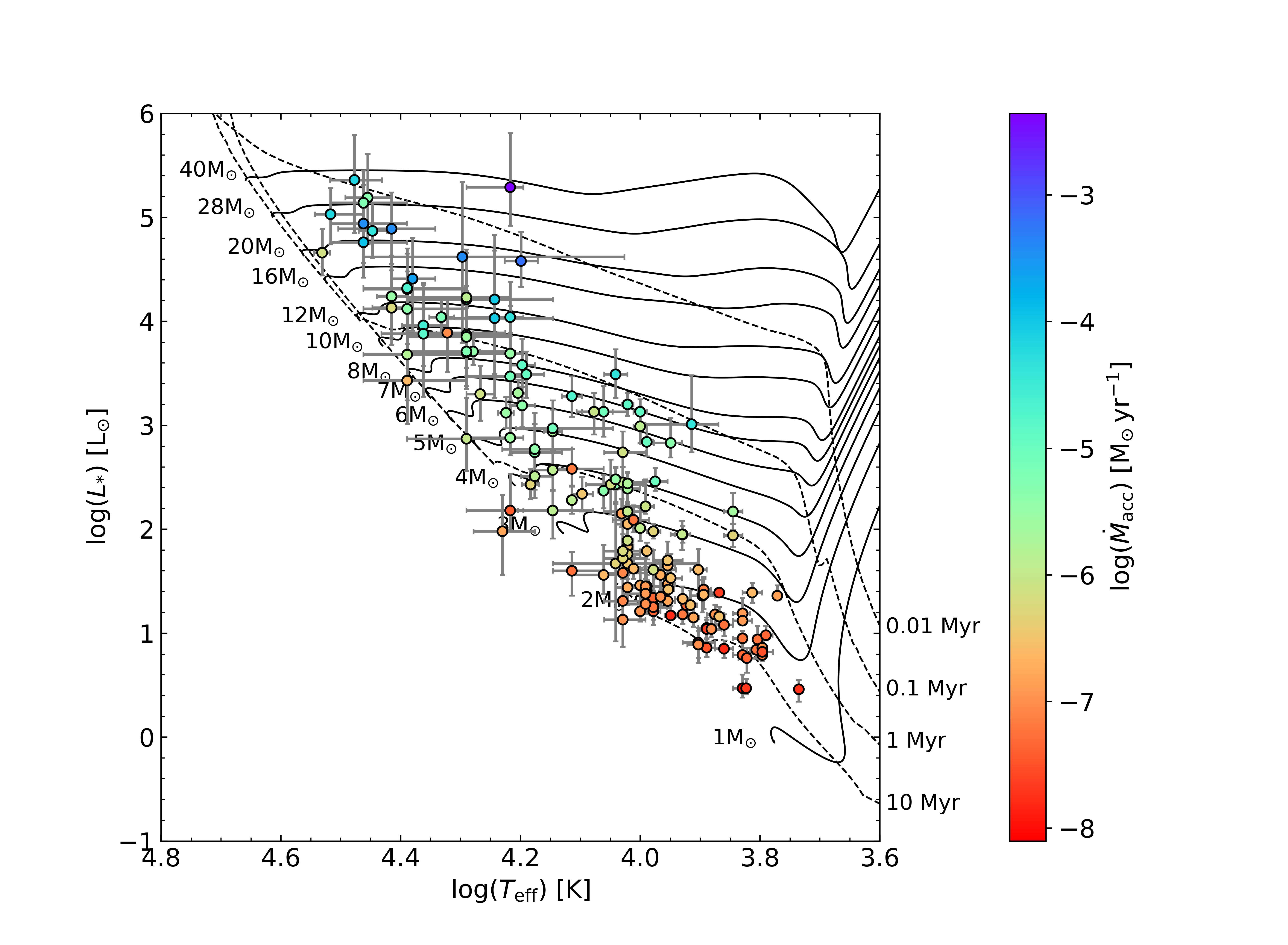
Figure 5: The placement of all 163 HAeBes in the HR diagram. The PMS tracks with initial mass from 1 to 40 $\rm M_{\sun}$ (Bressan et al., 2012; Tang et al., 2014) and isochrones of 0.01, 0.1, 1 and 10 Myr (Marigo et al., 2017) are plotted as solid and dashed lines respectively. The colour map denotes the accretion rate.

Let us first consider the sample with homogeneously derived mass accretion rates, before investigating the full sample. The relationship between mass accretion rate and stellar mass of the combined sample from this work and Fairlamb et al. (2015, 2017) that are present in Thé et al. (1994, table 1), is shown in the left hand panel of Figure 7. The sample of Thé et al. (1994), contains the best established HAeBes, and is thus least contaminated by possible misclassified objects. It can be seen that the mass accretion rate increases with stellar mass, and that there is a different behaviour for objects with masses below and above the mass range with $\log(M_{*})=0.4$–0.6. This break is consistent with the major finding in F15 that the relationship between mass accretion rate and stellar mass shows a break around the boundary between Herbig Ae and Herbig Be stars. In particular, they found that the relationship between mass accretion rate and mass has a different slope for the lower and higher mass objects respectively. With our improved sample in hand, we can now revisit this finding and we determine the mass at which the break occurs with higher precision in the same way as we found the turnover luminosity earlier.

We found that the maximum slope difference is at the $4.4\,\sigma$ level for the Thé et al. sample at $\log(M_{*})=0.56^{+0.14}_{-0.14}$ or $M_{*}=3.61^{+1.38}_{-0.98}\,\rm M_{\sun}$. The uncertainty in the mass is decided where the difference in slope is 1$\sigma$ smaller than at maximum. If we focus on the total combined sample of 78 objects from this work and F15, the break is established at $\log(M_{*})=0.58^{+0.14}_{-0.14}$ or $M_{*}=3.81^{+1.46}_{-1.05}\,\rm M_{\sun}$ with the maximum gradient difference about $6.4\,\sigma$. as shown in the middle panel of Figure 7. It can be seen that this plot shows the same relationship as the one in the left-hand panel. When considering the full, combined sample of 163 objects from this work, F15 and V18 whose mass accretion rates are shown in the right-hand panel of Figure 7, the break is now found at the $\log(M_{*})=0.60^{+0.13}_{-0.12}$ or $M_{*}=3.98^{+1.37}_{-0.94}\,\rm M_{\sun}$ with the maximum difference of gradient about $6.6\,\sigma$.

We note that both the significance of the difference in slopes as well as the mass at which the break occurs increases with the number of objects. This could be due to the number of objects; especially as the Thé et al. (1994) sample is sparsely populated at the high mass end, which could increase the uncertainty on the resulting slope and thus lower the significance of the difference in slopes between high and low mass objects. Alternatively, it could be affected by a larger contamination of non-Herbig Be stars in the full sample. It is notoriously hard to differentiate between a regular Be star and a Herbig Be star. Given the low number statistics of the Thé et al. (1994) sample and the similarity of the break in mass of the other two samples, we will proceed with a break in slope at 4 M_⊙.

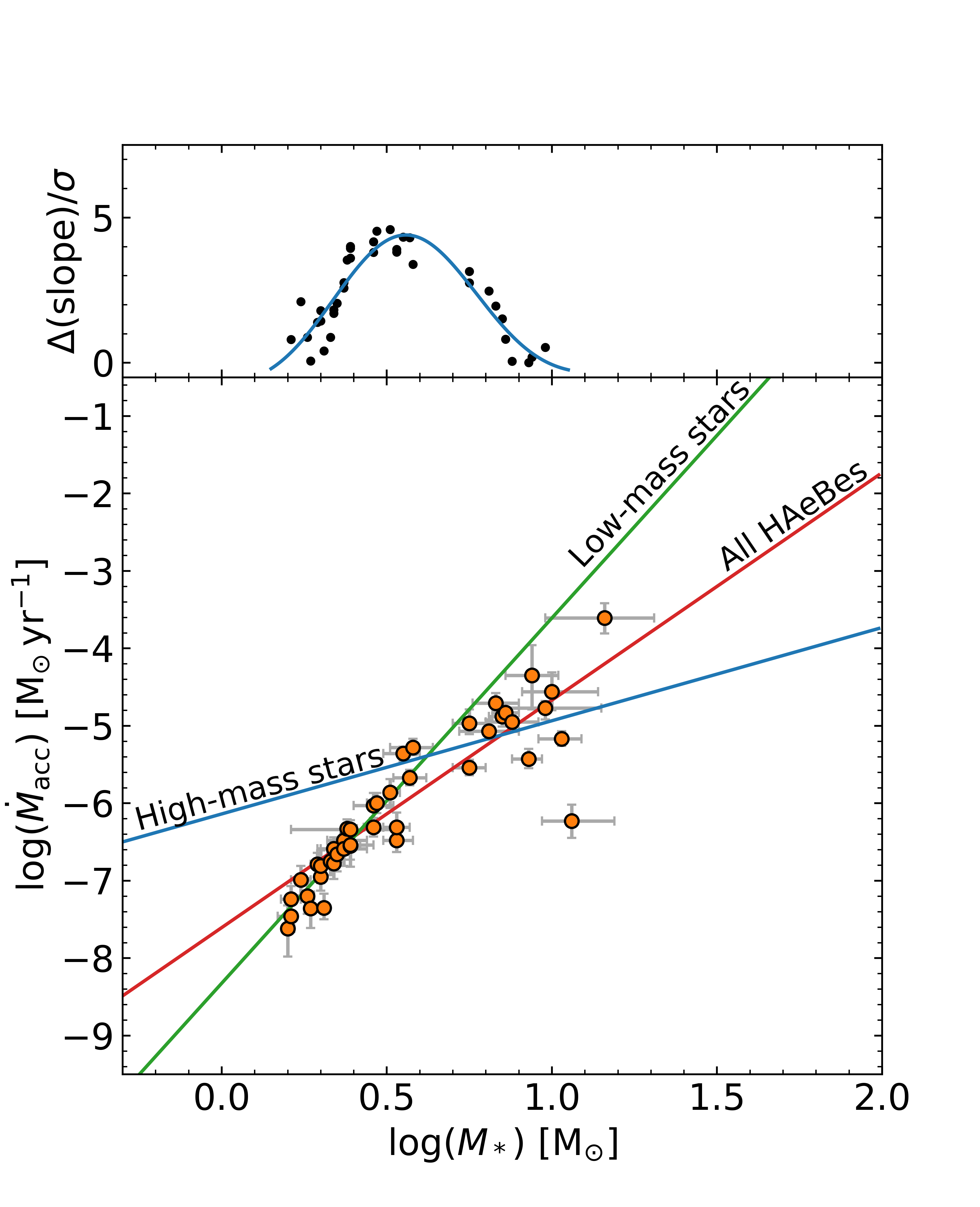
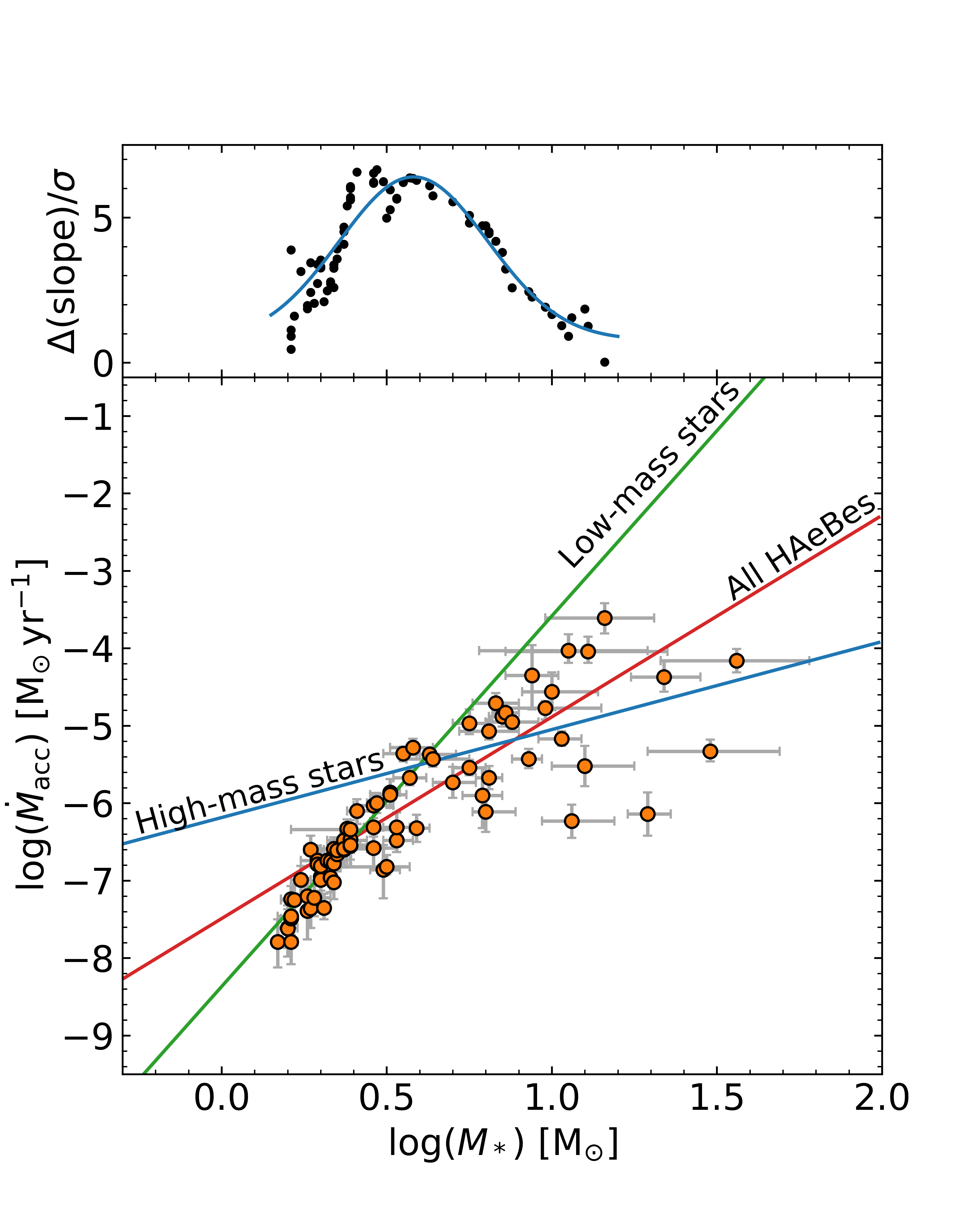
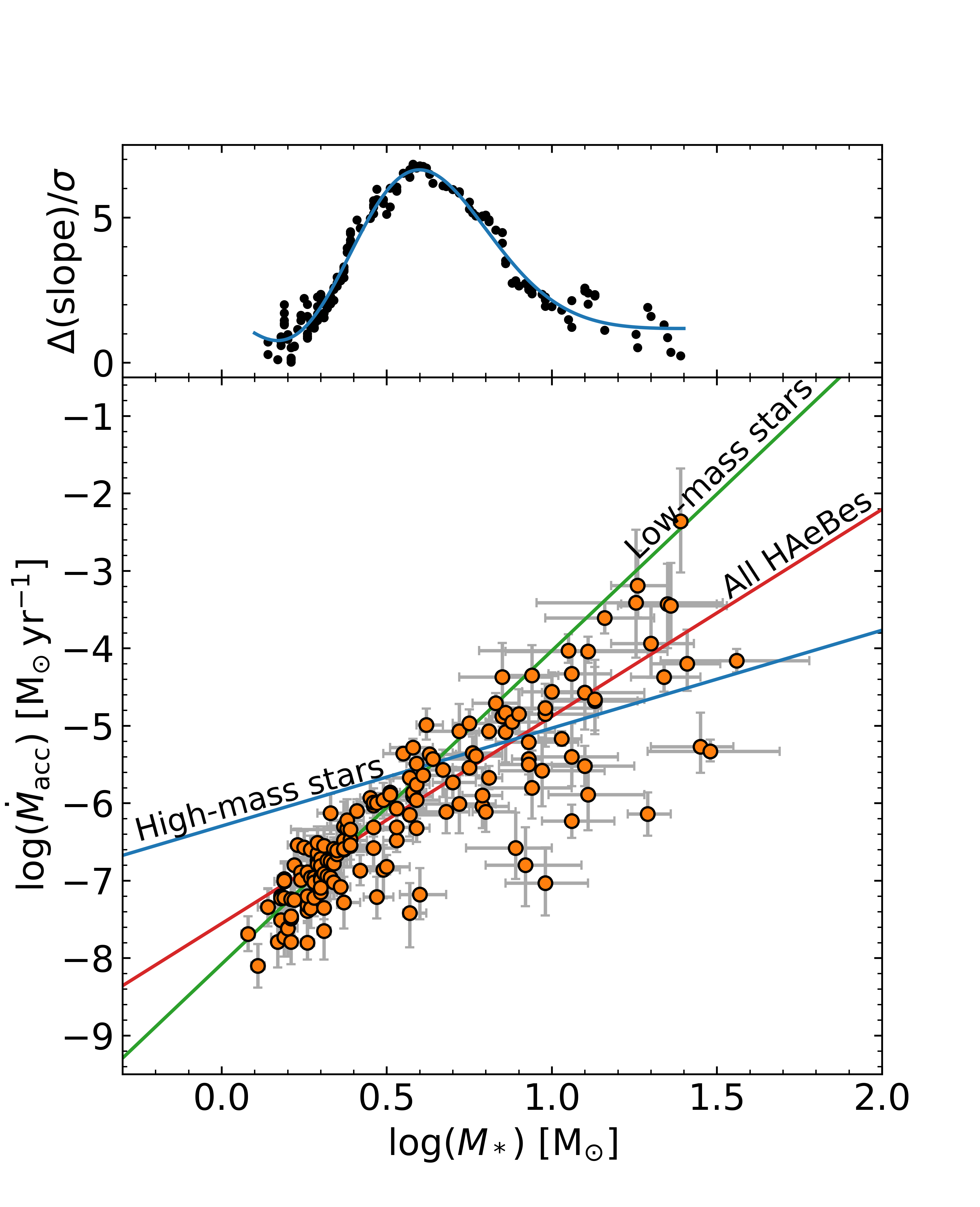
Figure 7: The difference of the gradient of the best fits between the low-mass and the high-mass HAeBes in terms of the uncertainty of the gradient difference (top panel) and the mass accretion rates versus stellar masses (bottom panel). Left: 43 stars from this work sample and the sample of Fairlamb et al. (2015) presents in table 1 of Thé et al. (1994). Objects are separated into the low-mass HAeBes, $M_{*}<3.61\,\rm M_{\sun}$, and the high-mass HAeBes, $M_{*}>3.61\,\rm M_{\sun}$. The slopes of best fits for the whole sample, low-mass and high-mass HAeBes are $2.94\pm 0.24$, $4.72\pm 0.49$ and $1.20\pm 0.65$ respectively. Middle: 78 objects from this work sample and the sample of Fairlamb et al. (2015). The break is defined at $M_{*}=3.81\,\rm M_{\sun}$. The gradients of best fits for the whole sample, low-mass and high-mass HAeBes are $2.60\pm 0.19$, $4.78\pm 0.34$ and $1.14\pm 0.46$ respectively. Right: 163 objects are separated into the low-mass HAeBes and the high-mass HAeBes at $M_{*}=3.98\,\rm M_{\sun}$. The gradients of best fits for the whole sample, low-mass and high-mass HAeBes are $2.67\pm 0.13$, $4.05\pm 0.24$ and $1.26\pm 0.34$ respectively.

5.2.1 Literature comparisons with T Tauri stars

It is interesting to see how the accretion luminosities compare to those of T Tauri stars at the low mass range. With the large caveat that no Gaia DR2 study of T Tauri stars and their stellar parameters and accretion rates exists at the moment, we show in Figure 8 the $L_{\rm acc}$ against $L_{*}$ for the whole sample of 163 HAeBes in this work compared to classical T Tauri stars of which all luminosity values are taken from Hartmann et al. (1998), White & Basri (2003), Calvet et al. (2004) and Natta et al. (2006). On one hand, the gradient of best fit for the classical T Tauri stars is $1.17\pm 0.09$ which is close, and well within the errorbars, to $1.03\pm 0.08$ for low-mass HAeBes. On the other hand, high-mass HAeBes shows a flatter relationship of $L_{\rm acc}\propto L^{0.60\pm 0.08}_{*}$. It would seem that the Herbig Ae and Be stars with masses up until 4 M_⊙ behave similarly to the T Tauri stars. Again, stellar parameters of these classical T Tauri stars were not derived in the same manner as HAeBes in this work. This may have an effect on our conclusion.

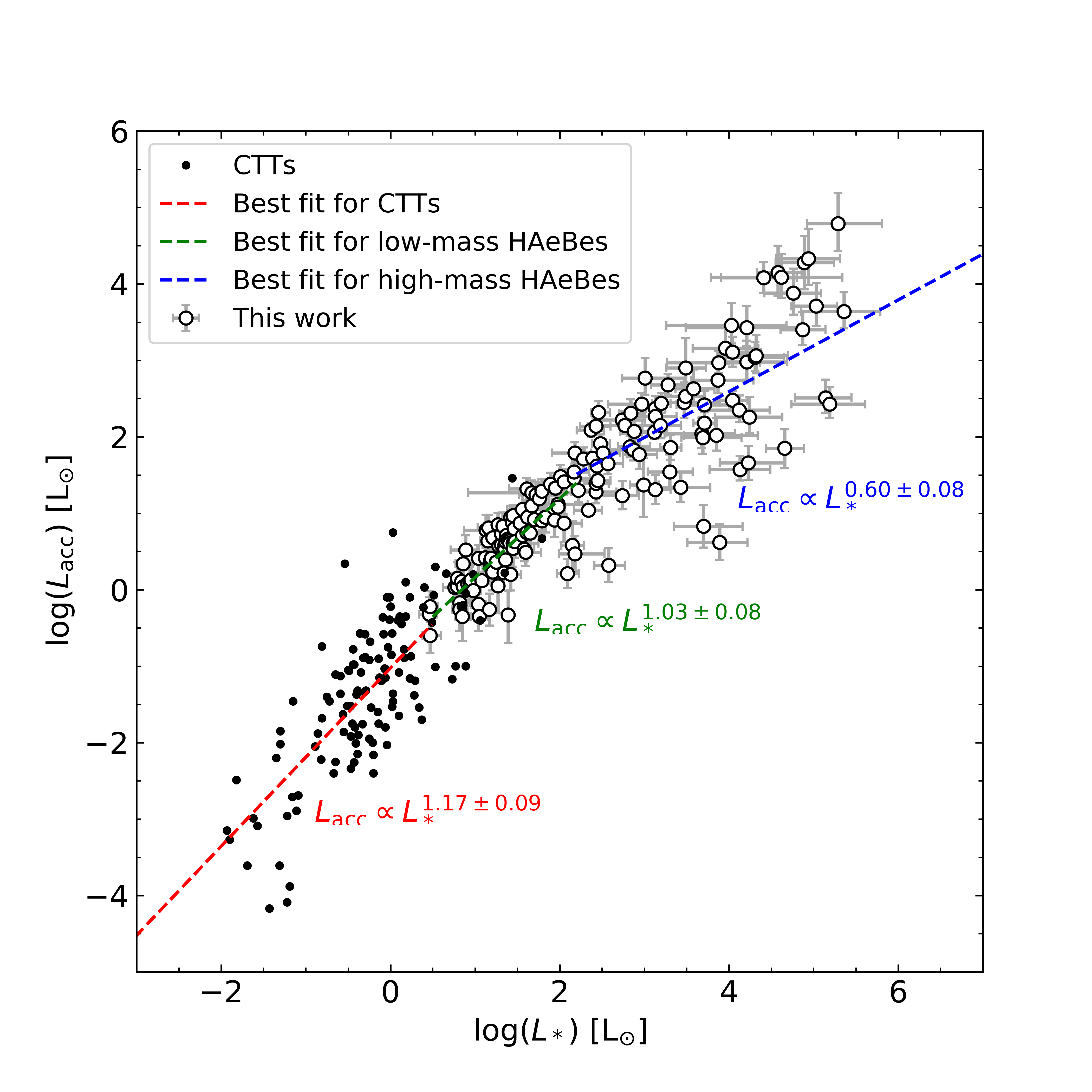
Figure 8: Accretion luminosity versus stellar luminosity for 163 HAeBes in this work and classical T Tauri stars from Hartmann et al. (1998), White & Basri (2003), Calvet et al. (2004) and Natta et al. (2006). Red, green and blue dashed lines are the best fit for T Tauri stars ($L_{\rm acc}\propto L^{1.17\pm 0.09}_{*}$), low-mass HAeBes ($L_{\rm acc}\propto L^{1.03\pm 0.08}_{*}$) and high-mass HAeBes ($L_{\rm acc}\propto L^{0.60\pm 0.08}_{*}$) respectively.

5.3 Mass accretion rate as a function of stellar age

In Figure 5 we illustrate the mass accretion rates across the HR-diagram. As expected, it can be seen that the accretion rates are largest for the brightest and most massive objects. However, the sample may allow an investigation into the evolution of the mass accretion rate as a function of stellar age as provided by the evolutionary models. In general it can be stated that, in terms of evolutionary age, the younger objects have higher accretion rates than older objects. As illustration, we show the mass accretion rate as a function of age in the top panel of Figure 9. It is clear that the accretion rate decreases with age (as also shown in F15); the Pearson correlation coefficient is -0.87.

However, when considering any properties as a function of age, there is always the issue that higher mass stars evolve faster than lower mass stars. Hence, the observed fact that higher mass objects have higher accretion rates could be the main underlying reason for a trend of decreasing accretion rate with time. Indeed, in the top panel of Figure 9 the range in accretion rates covers the entire accretion range of the accretion vs. mass relation, so it is hard to disentangle from this graph whether there is also an accretion rate - age relation.

This can in principle be circumvented when selecting a sample of objects in a small mass range, so that the spread in mass accretion rates is minimized. This needs to be offset against the number of objects under consideration. In the lower panels of Figure 9 we show how the accretion rate change with the age of stars in 3 different mass bins (2.0-$2.5\,\rm M_{\sun}$, 2.5-$3.0\,\rm M_{\sun}$ and 3.0-$3.5\,\rm M_{\sun}$. A best fit taken into account the uncertainties in both the mass accretion rate and age to the 30 objects where $2.0\,\rm M_{\sun}<M_{*}<2.5\,\rm M_{\sun}$ shows a $\dot{M}_{\rm acc}\propto Age^{-1.95\pm 0.49}$ with a Pearson’s correlation coefficient -0.55. The 9 stars with masses $2.5\,\rm M_{\sun}<M_{*}<3.0\,\rm M_{\sun}$ have a gradient of a best fit is $-1.40\pm 1.47$ (correlation coefficient 0.40). The error of the best fit gradient becomes slightly larger than its own value, which is due to the smaller number of objects involved. The 8 objects with $3.0\,\rm M_{\sun}<M_{*}<3.5\,\rm M_{\sun}$ in the bottom panel of Figure 9 have a gradient of a best fit is $-0.37\pm 1.25$ with a linear correlation -0.36. It can be seen that the error of the best fit gets larger than 3 times of its own absolute value. This is more likely to be due to the lack of HAeBes when the stellar mass increases.

The 2.0-2.5 M_⊙ sample is best suited to study any trend in accretion rate with age in the sense that the accretion rates change by 0.4 dex across this mass range (cf. the slope of 4.05 found for the low mass objects in Sec. 5.2). The spread in accretion rates in the graph is twice that, and if the additional decrease in mass accretion rate is due to evolution, we find $\dot{M}_{\rm acc}\propto Age^{-1.95\pm 0.49}$. This value is the only such determination for Herbig Ae/Be stars in a narrow mass range, other determinations were based on full samples of HAeBe stars which contain many different masses and suffer from a mass-age degeneracy (e.g. F15, Mendigutía et al. (2012)). Despite the relatively large errorbars, we note that our determination is remarkably close to the observed values for T Tauri stars by Hartmann et al. (1998), who find an $\eta$ between 1.5-2.8, while theoretically these authors predict $\eta$ to be larger than 1.5 for a single $\alpha$ viscous disk. We also refer the reader to the discussion in Mendigutía et al. (2012), who, remarkably, find a similar value of the exponent to ours: 1.8${}^{+1.4}_{-0.7}$ as determined for their full sample.

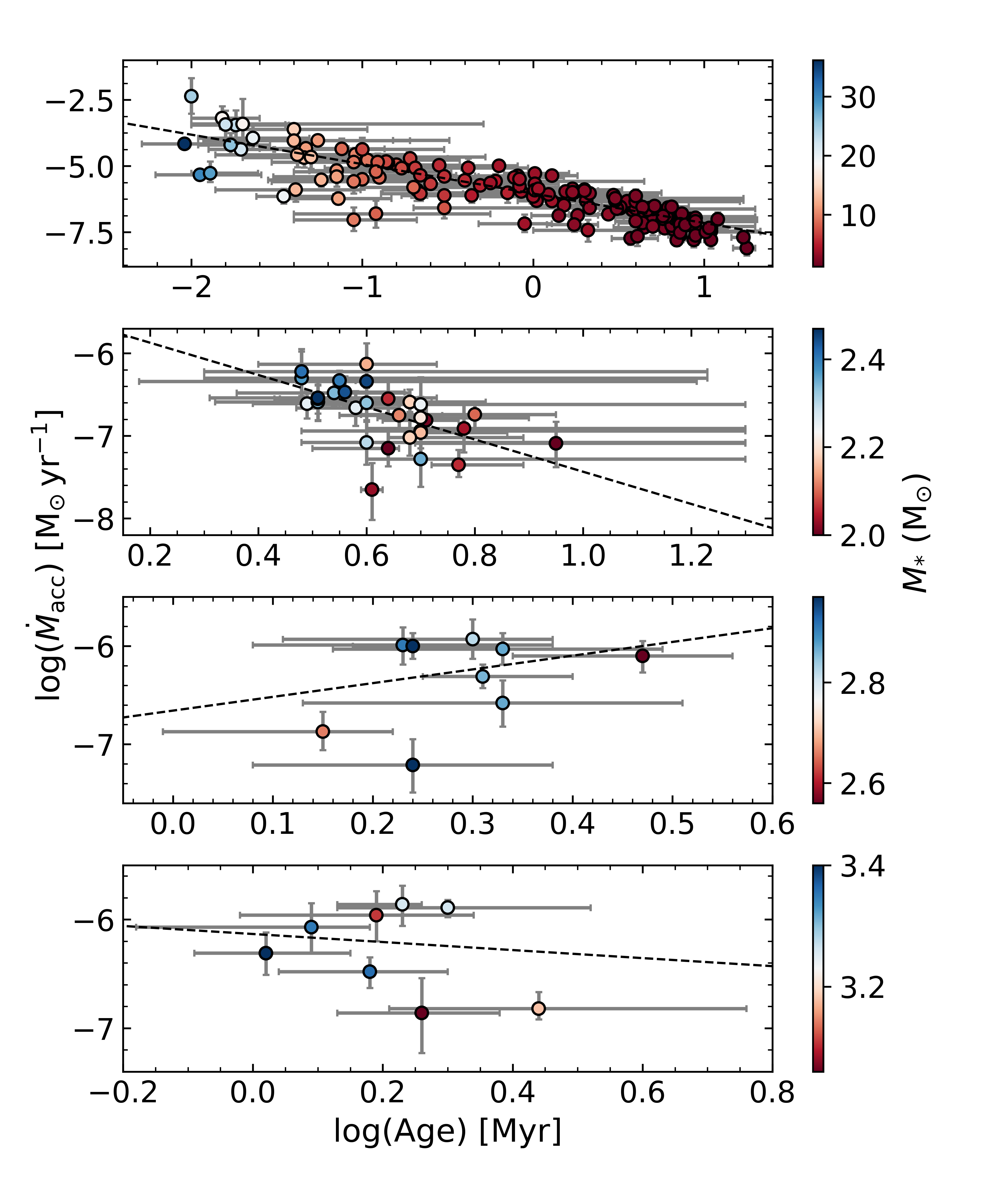
Figure 9: Ages versus mass accretion rates. From top to bottom all sample, the mass range 2.0-$2.5\,\rm M_{\sun}$, 2.5-$3.0\,\rm M_{\sun}$ and 3.0-$3.5\,\rm M_{\sun}$. The best fit is shown in the dashed line where $\dot{M}_{\rm acc}\propto Age^{-1.11\pm 0.05}$, $\dot{M}_{\rm acc}\propto Age^{-1.95\pm 0.49}$, $\dot{M}_{\rm acc}\propto Age^{1.40\pm 1.47}$ and $\dot{M}_{\rm acc}\propto Age^{-0.37\pm 1.25}$ respectively. The colour map indicates stellar mass of each mass bin.

6 Discussion

In the above we have worked out the mass accretion rates for a large sample of 163 Herbig Ae/Be stars. To this end new and spectroscopic archival data were employed. A large fraction of the sample now has homogeneously determined astrophysical parameters, while Gaia parallaxes were used to arrive at updated luminosities for the sample objects. We compared the mass accretion rates derived using the MA paradigm for Herbig Ae/Be stars with various properties. We find that:

• The mass accretion rate increases with stellar mass, but the sample can be split into two subsets depending on their masses.

• The low mass Herbig Ae stars’ accretion rates have a steeper dependence on mass than the higher mass Herbig Be stars.

• The above findings corroborate previous reports in the literature. The larger sample and improved data allows us to determine the mass where the largest difference in slopes between high and low mass objects occurs. We find it is 4 M_⊙.

• Bearing in mind the caveat that T Tauri stars do not yet have Gaia based accretion rates, it appears that the Herbig Ae stars’ accretion properties display a similar dependence on luminosity as the T Tauri stars.

• In general, younger objects have larger mass accretion rates, but it proves not trivial to disentangle a mass dependence from an age dependence. We present the first attempt to do so. A small subset in a narrow mass range leads us to suggest that the accretion rate decreases with time.

In the following we aim to put these results into context, but we start by discussing the various assumptions that had to be made to arrive at these results.

6.1 On the viability of the MA model to determine accretion rates of Herbig Ae/Be stars

In the above we have determined accretion luminosities and accretion rates to young stars. However, the question remains whether the magnetic accretion shock modelling that underpins these computations should be applicable. After all, A and B-type stars typically do not have magnetic field detections, and indeed, are not expected to harbour magnetic fields as their radiative envelopes would not create a dynamo that in turn can create a magnetic field. This was verified in a study of Intermediate Mass T Tauri stars (IMTTS) by Villebrun et al. (2019) who found that the fraction of pre-Main Sequence objects with a magnetic field detection drops markedly as they become hotter (for similar masses). These authors suspect that any B-field detections in Herbig Ae/Be stars could be fossil fields from the evolutionary stage immediately preceding them. The fields would not only be weaker, but also more complex, hampering their direct detection.

Muzerolle et al. (2004) showed that the MA models provided qualitative agreement with the observed emission line profiles of the Herbig Ae star UX Ori. In the process, they also found that the B-field geometry should be more complex than the usual dipole field in T Tauri stars and the expected field strength would be much below the usual T Tauri detections, in line with the Villebrun et al. (2019) findings.

Since, based on statistical studies and targeted individual investigations evidence has emerged that Herbig Ae stars are similar to the T Tauri stars. Garcia Lopez et al. (2006) showed that the accretion rate properties of the Herbig Ae stars constitute a natural extension to the T Tauri stars, while F15 demonstrated that the MA model can reproduce the observed UV excesses towards most of their Herbig Ae/Be stars with realistic parameters for the shocked regions. A small number of objects, all Herbig Be stars, could not be explained with the MA model. They exhibit such a large UV-excess that they would require shock covering factors larger than 100%, which is clearly unphysical.

Vink et al. (2002) and Vink et al. (2005) were the first to point out the remarkable similarity in the observed linear spectropolarimetric properties of the H$\alpha$ line in Herbig Ae stars and T Tauri stars. The polarimetric line effects in these types of objects can be explained with geometries consistent with light scattering off (magnetically) truncated disks. In contrast, the very different effects observed towards the Herbig Be stars were more consistent with disks reaching onto the central star - hinting at a different accretion mechanism in those. The large sample by Ababakr et al. (2017) allowed them to identify the transition region to be around spectral type B7/8.

Cauley & Johns-Krull (2014) studied the He i 1.083 $\mu$m line profiles of a large sample of Herbig stars and found that both T Tauri and Herbig Ae stars could be explained with MA, while the Herbig Be stars could not. Reiter et al. (2018) did not detect a difference in line morphology between the few (5) magnetic Herbig Ae/Be stars and the rest of the sample. They argued that Herbig Ae stars may therefore not accrete similarly to T Tauri stars. However, based on Poisson statistics alone, even if all magnetic objects showed either a P Cygni or Inverse P Cygni profile, a sample of 5 would not be sufficient to conclusively demonstrate that the magnetic objects are, or are not, different from the non-magnetic objects. Clearly, more work needs to be done in this area. Costigan et al. (2014) investigated the H$\alpha$ line variability properties of Herbig Ae/Be stars and T Tauri stars and found that both the timescales and amplitude of the variability were similar for the Herbig Ae and T Tauri, which also led these authors to suggest that the mode of accretion of these objects are similar. A notion also implied by our result in Figure 8 that the accretion luminosities of both Herbig Ae and T Tauri stars appear to have the same dependence on the stellar luminosity. Finally, Mendigutía et al. (2011a) found that the H$\alpha$ line width variability of Herbig Be stars is considerably smaller than for Herbig Ae stars, which is in turn smaller than for TTs (see Figure 37 in Fang et al. 2013). This may suggest smaller line emitting regions/magnetospheres as the stellar mass increases, and thus a eventual transition from MA to some other mechanism responsible for accretion.

To summarize this section, various studies of different observational properties have confirmed the many similarities between T Tauri and Herbig Ae stars, which in turn hint at a similar accretion mechanism, the magnetically controlled accretion. In turn, this would validate our use of the MA shock modelling to derive mass accretion rates for at least the lower mass end of the Herbig Ae/Be star range. Before we discuss the accretion mechanisms for low- and high mass stars, we address the use of line luminosities to arrive at accretion luminosities and rates below.

6.2 On the use of line emission as accretion rate diagnostic

The only “direct” manner to determine the mass accretion rate is to measure the accretion luminosity, which is essentially the amount of gravitational potential energy that is converted into radiation at ultra-violet wavelengths. This can then be turned into a mass accretion rate once the stellar mass and radius are known. The determination of the contribution of the accretion shock to the total UV emission for HAeBe objects is not straightforward due to the fact that these stars intrinsically emit many UV photons by virtue of their higher temperatures.

Calvet et al. (2004) showed that the Br$\gamma$ emission strengths observed towards a sample of IMTTS correlated with the accretion luminosity as determined by the UV excess for a large mass range extending to 3.7 M_⊙ (the mass of their most massive target, GW Ori, with spectral type G0 - cool enough to unambiguously determine the UV excess emission). This was already known for lower mass objects, but, significantly, these authors extended it to higher masses. In addition, these authors also showed that the mass accretion rate correlated with the stellar mass over this mass range. Therefore they also demonstrated that line emission, in this case the hydrogen recombination Br$\gamma$, can be used to measure accretion rates to masses of at least up to $\sim$4 M_⊙. Mendigutía et al. (2011b) measured the UV-excess of Herbig Ae/Be stars using UV-blue spectroscopy and photometry respectively and noted the correlation with emission line strengths (see also Donehew & Brittain 2011). F15 and F17 took this further and demonstrated the strong correlation between emission line strength and accretion luminosity for a much larger sample and a mass range going up to 10–15 M_⊙. It extended to an accretion luminosity of 10⁴ L_⊙ and was shown to hold for a large number of different emission lines.

One should keep in mind the caveat, also pointed out by F17, that high spatial resolution optical and near-infrared studies of the hydrogen line emission do not necessarily identify the line emitting regions of Herbig Ae/Be stars with the magnetospheric accretion channels. Already in 2008, Kraus et al. (2008) reported that their milli-arcsec resolution AMBER interferometric data indicated different Br$\gamma$ line forming regions which were consistent with the MA scenario for some objects but with disk-winds for others. Further studies by e.g. Mendigutía et al. (2015b) find the line emission region consistent with a rotating disk. Similarly, Tambovtseva et al. (2016) and Kreplin et al. (2018) find the disk-wind a more likely explanation for the emitting region than the compact accretion channels. Even higher resolution H$\alpha$ CHARA data discussed by Mendigutía et al. (2017) present a similar diversity.

There thus remains the question whether we can use emission lines to probe accretion if they are apparently not related to the accretion process itself, or indeed, why the line luminosities correlate with the accretion luminosity at all. It is well known that accretion onto young stars drives jets and outflows, where the mass ejection rates are of order 10% of the accretion rates (see e.g. Purser et al. 2016). If this is also the case for Herbig Ae/Be stars, then one could expect the emission lines to be correlated with the accretion rates. On the other hand, Mendigutía et al. (2015a) pointed out that while the physical origin of the lines may not be related to the accretion process per se, it is the underlying correlation between accretion luminosity and stellar luminosity that gives rise to a correlation between the line strengths and accretion. Hence, although the lines may not necessarily be directly accretion-related, the empirical correlations between emission line luminosities and accretion luminosities are strong enough to validate their use as accretion tracers.

When we revisit the various studies mentioned above, it is notable that a distinction between Herbig Ae and Herbig Be stars is found, spectroscopically (Cauley & Johns-Krull, 2014), spectropolarimetrically (Vink et al., 2005), due to spectral variability (Costigan et al., 2014), and even when considering the accretion rates from UV-excesses (F15).

Based on the break in accretion rates, we can move this boundary to a critical mass of 4M_⊙, remarkably close, but not perfectly so, to the boundary of around B7/8 put forward by Ababakr et al. (2017). It is thus implied that there is a transition from magnetically controlled accretion in low-mass HAeBes to another accretion mechanism in high-mass HAeBes at around $4\,\rm M_{\sun}$. The remaining question is what this mechanism should be.

6.3 If MA does not operate in massive objects, what then?

The spectropolarimetric finding of a disk reaching onto the star is reminiscent of the Boundary Layer (BL) accretion mechanism that was found to be a natural consequence of a viscous circumstellar disk around a stellar object (Lynden-Bell & Pringle 1974). The BL is a thin annulus close to the star in which the material reduces its (Keplerian) velocity to the slow rotation of the star when it reaches the stellar surface. It is here that kinetic energy and angular momentum will be dissipated. The BL mechanism was originally used to explain the observed UV excesses of low mass pre-Main Sequence stars (Bertout et al. 1988) until observations led to strong support for the magnetic accretion scenario instead (Bouvier et al. 2007). One of the difficulties the BL mechanism had was the smaller redshifted absorption linewidths predicted from the Keplerian widths expected from the BL than from freefall in the case of MA (Bertout et al. 1988). It had been suggested in the past to operate in Herbig Ae/Be objects (eg Blondel & Djie 2006 who studied Herbig Ae stars; Mendigutía et al. 2011b; Cauley & Johns-Krull 2014) but has never been adapted and tested for masses of Herbig Be stars and greater.

It is very much beyond the scope of this paper to address the BL theoretically, but let us suffice with a basic consideration to see whether we would be able to expect a different slope in the derived accretion rate or luminosity for an object undergoing MA or BL accretion. In both situations infalling material converts energy into radiation. In MA the energy released by a mass $dM$ falling onto a star with mass and radius $M_{*}$ and $R_{*}$ respectively will be the gravitational potential energy of the infalling material, $\frac{GM_{*}dM}{R_{*}}$, times a factor close to 1 accounting for the fact that material is not falling from infinity.

How would this amount of released energy compare to that in the BL scenario for infalling material of the same mass $dM$? For the BL case, the accretion energy will be at most the kinetic energy of the rotating material prior to being decelerated in the very thin layer close to the stellar surface. As the material rotates Keplerian, we know that the centripetal force equals the force of gravity, $\frac{dMv^{2}}{R_{*}}=\frac{GM_{*}dM}{R_{*}^{2}}$. We thus find that the kinetic energy $\frac{1}{2}dMv^{2}=\frac{GM_{*}dM}{2R_{*}}$, which is half the gravitational potential energy for the same mass.

In other words, the energy released in the BL scenario will be less than that released by MA for the same mass. Therefore if the mass accretion rate is the same, we obtain a lower accretion luminosity for objects accreting material through a Boundary Layer than through Magnetospheric Accretion. This also means that the accretion rate has to be larger in BL to arrive at the same accretion luminosity. In turn, this has as implication that if we derive the mass accretion rates using the MA paradigm, while the accretion is due to BL, then the resulting accretion luminosities and rates would have been underestimated.

Earlier, we found that the (MA derived) accretion luminosities have the same dependence of the accretion luminosity on the stellar luminosity for T Tauri stars and Herbig Ae stars, while we find a smaller gradient for the more massive stars. If we would assume that this dependence would hold for more massive stars too, then it could be concluded that the accretion rates have been underestimated for massive Herbig Be stars. If the BL scenario was the acting mechanism for the Herbig Be stars then the accretion luminosities would be larger - possibly resulting in the same relationship between accretion and stellar luminosity as the lower mass stars, and no break would be visible.

Could that be the case here? The accretion onto the stars likely depends on the rates the accretion disks are fed and mass needs to be transported through the disk, so it may be reasonable to assume that this process is less dependent on the stellar parameters and a simple correlation between accretion onto the star and stellar luminosity (or mass) would be expected. It is intriguing that the BL scenario for more massive stars might explain why we obtain lower accretion rates when we assume MA for the more massive objects resulting in a break at around $4\,\rm M_{\sun}$. An in-depth investigation into the BL is certainly warranted.

7 Final Remarks

In this paper we presented an analysis of a new set of optical spectroscopy of 30 northern Herbig Ae/Be stars. This was combined with our data and analysis of southern objects in F15 resulting in a set of temperatures, gravities, extinctions and luminosities that were derived in a consistent manner. As such this constitutes the largest homogeneously analysed sample of 78 Herbig Ae/Be stars to date. To these we added 85 objects from the Gaia DR2 study of V18. The total sample of 163 objects allowed us to derive the accretion luminosities and mass accretion rates using the empirical power-law relationship between accretion luminosity and line luminosity as derived under the MA paradigm.

We identified a subset in the total sample as being the strongest Herbig Ae/Be star candidates known. The set contains 60 per cent of the objects in Table 1 from the Thé et al. (1994) catalogue. All trends found in the large sample are also present in this subsample. This implies that the large sample likely has a low contamination and is therefore a good representation of the Herbig Ae/Be class.

• We find that the mass accretion rate increases with stellar mass, and that the lower mass Herbig Ae stars’ accretion rates have a steeper dependence on mass than the higher mass Herbig Be stars. This confirms previous findings, but the large sample allows us to determine the mass where this break occurs. This is found to be $4\,\rm M_{\sun}$.

• A comparison of accretion luminosities of the Herbig Ae/Be stars with those of T Tauri stars from the literature indicates that the Herbig Ae stars’ accretion rates display a similar dependence on luminosity as the T Tauri stars. This provides further evidence that Herbig Ae stars may accrete in a similar fashion as the T Tauri stars. We do caution however that T Tauri stars do not yet have Gaia-based accretion rates.

• We also find that in general, younger objects have larger mass accretion rates. However, it is not trivial to disentangle a mass and age dependence from each other: More massive stars have larger accretion rates, but have much smaller ages as well. A small subset selected in a narrow mass range leads us to suggest that the accretion rate does indeed decrease with time. The best value could be determined for the mass range 2.0-2.5 M_⊙. We find $\dot{M}_{\rm acc}\propto Age^{-1.95\pm 0.49}$.

Finally, we discussed the similarities and differences between the accretion properties of lower mass and higher mass Herbig pre-Main Sequence stars. In particular we discuss the various lines of evidence that suggest they accrete in different fashions. In addition, from linear spectropolarimetric studies, the Herbig Be stars are found to have disks reaching onto the stellar surface while the Herbig Ae stars (with the break around 4 M_☉) have disks with inner holes, similar to the T Tauri stars.

We therefore put forward the Boundary Layer mechanism as a viable manner for the accretion onto the stellar surface of massive pre-Main Sequence stars. More work needs to be done, but an initial, crude, estimate of the accretion luminosity dependency on mass – assuming a global correlation between mass accretion rate and stellar mass for all masses – can explain the observed break in accretion properties.

8 Supporting Information

Supplementary appendices are available for download alongside this article on the MNRAS website (https://academic.oup.com/mnras).

Table 2, 3, C1, C2 and D are available in electronic form at https://cdsarc.unistra.fr/viz-bin/cat/J/MNRAS/493/234.

Table A1: Log of observations of standard stars. Column 1 gives the object name. Columns 2 and 3 are right ascension (RA) in the units of time ($\aas@@fstack{h}$  $\aas@@fstack{m}$  $\aas@@fstack{s}$) and declination (DEC) in the units of angle ($\aas@@fstack{\circ}$  $\aas@@fstack{\prime}$  $\aas@@fstack{\prime\prime}$) respectively, column 4 lists the observation dates. Columns 5–7 present the exposure times for each grating. The signal-to-noise ratios for each grating are given in columns 8–10. Spectral type is listed along with references in columns 11–12.

Name	RA	DEC	Obs Date	Exposure Time (s)			SNR			Spectral Type
	(J2000)	(J2000)	(June 2013)	R1200B	R1200Y	R1200R	R1200B	R1200Y	R1200R		Ref.
Feige 98	14:38:15.8	+27:29:33.0	23	-	300	-	-	94	-	sdB9III:He1	1
HD 130109	14:46:14.9	+01:53:34.4	21; 23	60; 20	20	-	179	420	-	A0 IIInn	2
BD+26 2606	14:49:02.4	+25:42:09.2	23	-	150	-	-	124	-	A5	3
HD 147394	16:19:44.4	+46:18:48.1	21; 23	20	20; 10	-	319	376	-	B5 IV	4
HD 152614	16:54:00.5	+10:09:55.3	20; 22; 24	30	15	30; 15	257	339	179	B8 V	5
HD 153653	17:00:29.4	+06:35:01.3	20; 22; 24	60	40	15; 30	36	247	69	A7 V	6
HD 157741	17:24:33.8	+15:36:21.8	22; 23; 24	-	40; 30	40	-	534	157	B9 V	6
HD 158485	17:26:04.8	+58:39:06.8	21; 23	60	60	-	52	439	-	A4 V	6
HD 160762	17:39:27.9	+46:00:22.8	21; 23	20	10; 5	-	247	302	-	B3 IV	7
HD 161056	17:43:47.0	-07:04:46.6	23	-	30	-	-	464	-	B3 Vn	8
HD 175426	18:53:43.6	+36:58:18.2	20; 22; 24	60	40	40	245	390	204	B2 V	9
HD 177724	19:05:24.6	+13:51:48.5	21; 23; 25	20; 15	10	10	184	224	395	A0 IV-Vnn	10
HD 186307	19:41:57.6	+40:15:14.9	25	-	-	60	-	-	125	A6 V	6
HD 196504	20:37:04.7	+26:27:43.0	25	-	-	40	-	-	235	B8 V	11
HD 199081	20:53:14.8	+44:23:14.1	21; 23; 25	20	20	20; 60	234	492	118	B5 V	7

References: (1) Drilling et al. (2013); (2) Abt & Morrell (1995); (3) Fulbright (2000); (4) Morgan & Keenan (1973); (5) Cowley (1972); (6) Cowley et al. (1969); (7) Lesh (1968); (8) De Vaucouleurs (1957); (9) Hill & Lynas-Gray (1977); (10) Gray et al. (2003); (11) Hube (1970).

Figure B1: The $\rm H\alpha$ line profiles for the 30 objects listed in Table 1.

Figure B1: continued

.

Table C1: Stellar parameters of 91 Herbig Ae/Be stars in the Fairlamb et al. (2015) sample. Column 1 gives the object name. Columns 2 and 3 are right ascension (RA) in the units of time ($\aas@@fstack{h}$  $\aas@@fstack{m}$  $\aas@@fstack{s}$) and declination (DEC) in the units of angle ($\aas@@fstack{\circ}$  $\aas@@fstack{\prime}$  $\aas@@fstack{\prime\prime}$) respectively. Columns 4–11 are effective temperature, surface gravity, visual extinction, distance, radius, luminosity, mass and age respectively. Temperature and surface gravity are taken from Fairlamb et al. (2015). Distance is obtained from Vioque et al. (2018). The rest of parameters are redetermined in this work. This table is available in electronic form at https://cdsarc.unistra.fr/viz-bin/cat/J/MNRAS/493/234.

Name	RA	DEC	$T_{\rm eff}$	$\log(g)$	$A_{V}$	D	$R_{*}$	$\log(L_{*})$	$M_{*}$	Age
	(J2000)	(J2000)	(K)	[cm s-2]	(mag)	(pc)	($\rm R_{\sun}$)	[$\rm L_{\sun}$]	($\rm M_{\sun}$)	(Myr)
UX Ori	05:04:29.9	-03:47:14.2	$8500^{+250}_{-250}$	$3.90^{+0.25}_{-0.25}$	$0.99^{+0.04}_{-0.03}$	$324.9^{+9.3}_{-8.4}$	$1.80^{+0.09}_{-0.08}$	$1.18^{+0.09}_{-0.09}$	$1.82^{+0.07}_{-0.08}$	$7.08^{+0.51}_{-0.47}$
PDS 174	05:06:55.5	-03:21:13.3	$17000^{+2000}_{-2000}$	$4.10^{+0.40}_{-0.40}$	$3.36^{+0.29}_{-0.39}$	$398^{+10}_{-9}$	$1.12^{+0.23}_{-0.23}$	$1.98^{+0.35}_{-0.42}$	$3.18^{+0.57}_{-0.87}$	$2.75^{+3.01}_{-1.13}$
V1012 Ori	05:11:36.5	-02:22:48.4	$8500^{+250}_{-250}$	$4.38^{+0.15}_{-0.15}$	$1.15^{+0.05}_{-0.06}$	-d	-	-	-	-
HD 34282	05:16:00.4	-09:48:35.3	$9500^{+250}_{-250}$	$4.40^{+0.15}_{-0.15}$	$0.55^{+0.03}_{-0.02}$	$311.5^{+7.9}_{-7.2}$	$1.48^{+0.06}_{-0.05}$	$1.21^{+0.08}_{-0.08}$	$1.87^{+0.11}_{-0.04}$	$8.91^{+2.89}_{-2.15}$
HD 287823	05:24:08.0	+02:27:46.8	$8375^{+125}_{-125}$	$4.23^{+0.11}_{-0.15}$	$0.39^{+0.03}_{-0.03}$	$359^{+12}_{-11}$	$2.06^{+0.11}_{-0.10}$	$1.27^{+0.07}_{-0.07}$	$1.80^{+0.07}_{-0.04}$	$6.61^{+0.64}_{-0.58}$
HD 287841	05:24:42.8	+01:43:48.2	$7750^{+250}_{-250}$	$4.27^{+0.12}_{-0.12}$	$0.33^{+0.03}_{-0.03}$	$366^{+10}_{-9}$	$1.85^{+0.08}_{-0.07}$	$1.04^{+0.09}_{-0.09}$	$1.60^{+0.07}_{-0.02}$	$8.91^{+0.64}_{-1.15}$
HD 290409	05:27:05.4	+00:25:07.6	$9750^{+500}_{-500}$	$4.25^{+0.25}_{-0.25}$	$0.41^{+0.03}_{-0.03}$	$455^{+31}_{-25}$	$1.87^{+0.16}_{-0.13}$	$1.45^{+0.16}_{-0.16}$	$2.18^{+0.01}_{-0.24}$	$4.79^{+2.97}_{-0.42}$
HD 35929	05:27:42.7	-08:19:38.4	$7000^{+250}_{-250}$	$3.47^{+0.11}_{-0.11}$	$0.35^{+0.05}_{-0.04}$	$387^{+13}_{-12}$	$6.39^{+0.38}_{-0.34}$	$1.94^{+0.11}_{-0.11}$	$3.40^{+0.31}_{-0.33}$	$1.05^{+0.36}_{-0.24}$
HD 290500	05:29:48.0	-00:23:43.5	$9500^{+500}_{-500}$	$3.80^{+0.40}_{-0.40}$	$1.03^{+0.06}_{-0.07}$ b	$438^{+24}_{-20}$	$1.56^{+0.14}_{-0.12}$	$1.25^{+0.16}_{-0.17}$	$1.89^{+0.21}_{-0.11}$	$8.13^{+4.77}_{-3.00}$
HD 244314	05:30:19.0	+11:20:20.0	$8500^{+250}_{-250}$	$4.15^{+0.11}_{-0.15}$	$0.51^{+0.06}_{-0.06}$	$432^{+19}_{-17}$	$2.14^{+0.17}_{-0.15}$	$1.33^{+0.12}_{-0.12}$	$1.86^{+0.16}_{-0.07}$	$6.17^{+0.91}_{-1.27}$
HK Ori	05:31:28.0	+12:09:10.1	$8500^{+500}_{-500}$	$4.22^{+0.13}_{-0.13}$	$1.31^{+0.20}_{-0.25}$	-e	-	-	-	-
HD 244604	05:31:57.2	+11:17:41.3	$9000^{+250}_{-250}$	$3.99^{+0.15}_{-0.13}$	$0.59^{+0.04}_{-0.05}$	$421^{+19}_{-17}$	$2.77^{+0.19}_{-0.18}$	$1.65^{+0.11}_{-0.11}$	$2.26^{+0.22}_{-0.16}$	$3.80^{+0.77}_{-0.85}$
UY Ori	05:32:00.3	-04:55:53.9	$9750^{+250}_{-250}$	$4.30^{+0.20}_{-0.20}$	$1.37^{+0.13}_{-0.14}$	-d	-	-	-	-
HD 245185	05:35:09.6	+10:01:51.4	$10000^{+500}_{-500}$	$4.25^{+0.25}_{-0.25}$	$0.40^{+0.03}_{-0.02}$	$429^{+37}_{-29}$	$1.78^{+0.19}_{-0.14}$	$1.46^{+0.17}_{-0.16}$	$2.21^{+0.04}_{-0.24}$	$5.01^{+2.93}_{-0.84}$
T Ori	05:35:50.4	-05:28:34.9	$9000^{+500}_{-500}$	$3.60^{+0.30}_{-0.30}$	$1.78^{+0.12}_{-0.13}$	$408^{+13}_{-11}$	$2.91^{+0.30}_{-0.27}$	$1.70^{+0.18}_{-0.18}$	$2.34^{+0.38}_{-0.27}$	$3.47^{+1.32}_{-1.18}$
V380 Ori	05:36:25.4	-06:42:57.6	$9750^{+750}_{-750}$	$4.00^{+0.35}_{-0.35}$	$2.05^{+0.26}_{-0.35}$	-d	-	-	-	-
HD 37258	05:36:59.2	-06:09:16.3	$9750^{+500}_{-500}$	$4.25^{+0.25}_{-0.25}$	$0.54^{+0.03}_{-0.04}$	-d	-	-	-	-
HD 290770	05:37:02.4	-01:37:21.3	$10500^{+250}_{-250}$	$4.20^{+0.30}_{-0.30}$	$0.34^{+0.05}_{-0.05}$	$399^{+21}_{-18}$	$2.08^{+0.17}_{-0.15}$	$1.67^{+0.11}_{-0.11}$	$2.44^{+0.05}_{-0.14}$	$3.63^{+1.05}_{-0.16}$
BF Ori	05:37:13.2	-06:35:00.5	$9000^{+250}_{-250}$	$3.97^{+0.15}_{-0.13}$	$0.74^{+0.06}_{-0.07}$	$389^{+14}_{-12}$	$2.25^{+0.16}_{-0.15}$	$1.47^{+0.11}_{-0.11}$	$2.01^{+0.15}_{-0.08}$	$5.13^{+0.76}_{-0.86}$
HD 37357	05:37:47.0	-06:42:30.2	$9500^{+250}_{-250}$	$4.10^{+0.10}_{-0.10}$	$0.40^{+0.03}_{-0.03}$	-d	-	-	-	-
HD 290764	05:38:05.2	-01:15:21.6	$7875^{+375}_{-375}$	$3.90^{+0.17}_{-0.15}$	$0.58^{+0.07}_{-0.08}$	$398^{+18}_{-15}$	$2.58^{+0.22}_{-0.20}$	$1.36^{+0.15}_{-0.16}$	$1.94^{+0.24}_{-0.20}$	$5.25^{+1.83}_{-1.36}$
HD 37411	05:38:14.5	-05:25:13.3	$9750^{+250}_{-250}$	$4.35^{+0.15}_{-0.15}$	$0.59^{+0.07}_{-0.07}$	-e	-	-	-	-
V599 Ori	05:38:58.6	-07:16:45.6	$8000^{+250}_{-250}$	$3.72^{+0.13}_{-0.12}$	$4.92^{+0.25}_{-0.35}$	$410^{+12}_{-11}$	$3.34^{+0.60}_{-0.62}$	$1.61^{+0.20}_{-0.23}$	$2.34^{+0.41}_{-0.39}$	$3.24^{+2.01}_{-1.15}$
V350 Ori	05:40:11.7	-09:42:11.0	$9000^{+250}_{-250}$	$4.18^{+0.11}_{-0.16}$	$1.06^{+0.08}_{-0.08}$	-d	-	-	-	-
HD 250550	06:01:59.9	+16:30:56.7	$11000^{+500}_{-500}$	$3.80^{+0.40}_{-0.40}$	$1.55^{+0.10}_{-0.13}$ b	$697^{+94}_{-64}$	$15.35^{+3.09}_{-2.38}$	$3.49^{+0.24}_{-0.23}$	$8.81^{+1.83}_{-1.51}$	$0.08^{+0.06}_{-0.03}$
V791 Mon	06:02:14.8	-10:00:59.5	$15000^{+1500}_{-1500}$	$4.30^{+0.16}_{-0.16}$	$1.48^{+0.11}_{-0.13}$	$887^{+53}_{-44}$	$3.47^{+0.44}_{-0.39}$	$2.74^{+0.27}_{-0.29}$	$4.31^{+0.92}_{-0.40}$	$0.81^{+0.42}_{-0.36}$
PDS 124	06:06:58.4	-05:55:06.7	$10250^{+250}_{-250}$	$4.30^{+0.20}_{-0.20}$	$1.79^{+0.02}_{-0.01}$	$853^{+64}_{-51}$	$2.06^{+0.18}_{-0.14}$	$1.62^{+0.11}_{-0.10}$	$2.33^{+0.02}_{-0.04}$	$3.98^{+0.59}_{-0.26}$
LkHa 339	06:10:57.8	-06:14:39.6	$10500^{+250}_{-250}$	$4.20^{+0.20}_{-0.20}$	$3.11^{+0.36}_{-0.54}$	$857^{+33}_{-29}$	$2.50^{+0.67}_{-0.67}$	$1.83^{+0.25}_{-0.31}$	$2.47^{+0.46}_{-0.27}$	$3.24^{+2.13}_{-1.20}$
VY Mon	06:31:06.9	+10:26:04.9	$12000^{+4000}_{-4000}$	$3.75^{+0.50}_{-0.50}$	$5.62^{+0.34}_{-0.51}$	-d	-	-	-	-
R Mon	06:39:09.9	+08:44:09.5	$12000^{+2000}_{-2000}$	$4.00^{+0.11}_{-0.24}$	$2.47^{+0.23}_{-0.29}$	-e	-	-	-	-
V590 Mon	06:40:44.6	+09:48:02.1	$12500^{+1000}_{-1000}$	$4.20^{+0.30}_{-0.30}$	$1.03^{+0.19}_{-0.24}$	-d	-	-	-	-
PDS 24	06:48:41.6	-16:48:05.6	$10500^{+500}_{-500}$	$4.20^{+0.30}_{-0.30}$	$1.45^{+0.10}_{-0.12}$	$1130^{+42}_{-37}$	$1.59^{+0.15}_{-0.15}$	$1.44^{+0.16}_{-0.17}$	$2.10^{+0.32}_{-0.12}$	$6.31^{+2.60}_{-2.42}$

Table C1: continued

. Name RA DEC $T_{\rm eff}$ $\log(g)$ $A_{V}$ D $R_{*}$ $\log(L_{*})$ $M_{*}$ Age (J2000) (J2000) (K) [cm s^-2] (mag) (pc) ($\rm R_{\sun}$) [$\rm L_{\sun}$] ($\rm M_{\sun}$) (Myr) PDS 130 06:49:58.5 -07:38:52.2 $10500^{+250}_{-250}$ $3.90^{+0.20}_{-0.20}$ $2.38^{+0.13}_{-0.15}$ $1316^{+62}_{-53}$ $2.68^{+0.34}_{-0.31}$ $1.89^{+0.14}_{-0.15}$ $2.56^{+0.28}_{-0.17}$ $2.95^{+0.68}_{-0.76}$ PDS 229 06:55:40.0 -03:09:50.5 $12500^{+250}_{-250}$ $4.20^{+0.20}_{-0.20}$ $2.24^{+0.15}_{-0.17}$ -^d - - - - GU CMa 07:01:49.5 -11:18:03.3 $22500^{+1500}_{-1500}$ $3.90^{+0.40}_{-0.40}$ $0.80^{+0.10}_{-0.12}$ -^e - - - - HT CMa 07:02:42.5 -11:26:11.8 $10500^{+500}_{-500}$ $4.00^{+0.20}_{-0.20}$ $1.61^{+0.09}_{-0.09}$ ^b $1121^{+83}_{-66}$ $3.19^{+0.41}_{-0.33}$ $2.05^{+0.19}_{-0.18}$ $2.87^{+0.44}_{-0.36}$ $2.14^{+0.95}_{-0.69}$ Z CMa 07:03:43.1 -11:33:06.2 $8500^{+500}_{-500}$ $2.53^{+0.17}_{-0.17}$ $3.09^{+0.23}_{-0.28}$ ^b -^d - - - - HU CMa 07:04:06.7 -11:26:08.5 $13000^{+250}_{-250}$ $4.20^{+0.20}_{-0.20}$ $1.29^{+0.07}_{-0.07}$ $1170^{+100}_{-80}$ $2.72^{+0.35}_{-0.28}$ $2.28^{+0.14}_{-0.13}$ $3.26^{+0.26}_{-0.02}$ $1.70^{+0.12}_{-0.35}$ HD 53367 07:04:25.5 -10:27:15.7 $29500^{+1000}_{-1000}$ $4.25^{+0.25}_{-0.25}$ $2.12^{+0.13}_{-0.14}$ -^d - - - - PDS 241 07:08:38.7 -04:19:04.8 $26000^{+1500}_{-1500}$ $4.00^{+0.30}_{-0.30}$ $2.92^{+0.27}_{-0.37}$ $2890^{+600}_{-400}$ $6.51^{+2.63}_{-1.90}$ $4.24^{+0.39}_{-0.40}$ $12.60^{+5.09}_{-2.58}$ $0.06^{+0.06}_{-0.03}$ NX Pup 07:19:28.2 -44:35:11.2 $7000^{+250}_{-250}$ $3.78^{+0.13}_{-0.13}$ $0.26^{+0.14}_{-0.17}$ -^d - - - - PDS 27 07:19:35.9 -17:39:17.9 $17500^{+3500}_{-3500}$ $3.16^{+0.27}_{-0.27}$ $4.96^{+0.33}_{-0.49}$ $2550^{+460}_{-310}$ $13.84^{+5.77}_{-4.42}$ $4.21^{+0.62}_{-0.72}$ $12.89^{+9.62}_{-5.67}$ $0.04^{+0.15}_{-0.03}$ PDS 133 07:25:04.9 -25:45:49.6 $14000^{+2000}_{-2000}$ $4.08^{+0.12}_{-0.11}$ $1.92^{+0.09}_{-0.10}$ $1475^{+92}_{-76}$ $2.09^{+-0.11}_{-0.01}$ $2.18^{+0.19}_{-0.27}$ $3.26^{+0.40}_{-0.39}$ $2.00^{+1.31}_{-0.65}$ HD 59319^c 07:28:36.7 -21:57:49.2 $12500^{+500}_{-500}$ $3.50^{+0.20}_{-0.20}$ $0.06^{+0.02}_{-0.01}$ $668^{+39}_{-33}$ $4.00^{+0.28}_{-0.22}$ $2.54^{+0.13}_{-0.12}$ $3.89^{+0.41}_{-0.36}$ $1.00^{+0.32}_{-0.26}$ PDS 134 07:32:26.6 -21:55:35.7 $14000^{+500}_{-500}$ $3.40^{+0.30}_{-0.30}$ $1.70^{+0.06}_{-0.07}$ $2550^{+370}_{-260}$ $5.00^{+0.92}_{-0.69}$ $2.94^{+0.21}_{-0.19}$ $5.05^{+0.94}_{-0.67}$ $0.49^{+0.25}_{-0.20}$ HD 68695 08:11:44.5 -44:05:08.7 $9250^{+250}_{-250}$ $4.40^{+0.15}_{-0.15}$ $0.37^{+0.05}_{-0.05}$ $396^{+10}_{-9}$ $1.86^{+0.10}_{-0.09}$ $1.35^{+0.09}_{-0.09}$ $1.98^{+0.11}_{-0.03}$ $5.76^{+0.70}_{-0.39}$ HD 72106 08:29:34.8 -38:36:21.1 $8750^{+250}_{-250}$ $3.89^{+0.13}_{-0.12}$ $0.00^{+0.03}_{-0.00}$ -^d - - - - TYC 8581-2002-1^c 08:44:23.6 -59:56:57.8 $9750^{+250}_{-250}$ $4.00^{+0.10}_{-0.10}$ $1.54^{+0.05}_{-0.07}$ $558^{+12}_{-11}$ $1.98^{+0.10}_{-0.11}$ $1.50^{+0.09}_{-0.09}$ $2.14^{+0.11}_{-0.03}$ $4.79^{+0.22}_{-0.32}$ PDS 33 08:48:45.6 -40:48:21.0 $9750^{+250}_{-250}$ $4.40^{+0.15}_{-0.15}$ $1.03^{+0.03}_{-0.02}$ $951^{+43}_{-37}$ $1.79^{+0.11}_{-0.09}$ $1.41^{+0.10}_{-0.09}$ $2.16^{+0.04}_{-0.19}$ $5.01^{+2.24}_{-0.33}$ HD 76534 08:55:08.7 -43:27:59.8 $19000^{+500}_{-500}$ $4.10^{+0.20}_{-0.20}$ $0.95^{+0.07}_{-0.08}$ $911^{+55}_{-46}$ $6.61^{+0.69}_{-0.60}$ $3.71^{+0.13}_{-0.13}$ $8.49^{+0.90}_{-0.88}$ $0.13^{+0.05}_{-0.03}$ PDS 281^c 08:55:45.9 -44:25:14.1 $16000^{+1500}_{-1500}$ $3.50^{+0.30}_{-0.30}$ $2.32^{+0.09}_{-0.09}$ $932^{+47}_{-40}$ $10.14^{+1.03}_{-0.90}$ $3.78^{+0.24}_{-0.25}$ $9.31^{+2.03}_{-1.70}$ $0.09^{+0.07}_{-0.04}$ PDS 286 09:06:00.0 -47:18:58.1 $30000^{+3000}_{-3000}$ $4.25^{+0.16}_{-0.16}$ $6.44^{+0.35}_{-0.56}$ $1820^{+210}_{-150}$ $17.72^{+6.33}_{-5.58}$ $5.36^{+0.43}_{-0.51}$ $36.13^{+24.39}_{-14.82}$ $0.01^{+0.01}_{-0.00}$ PDS 297 09:42:40.3 -56:15:34.1 $10750^{+250}_{-250}$ $4.00^{+0.20}_{-0.20}$ $1.23^{+0.06}_{-0.06}$ $1590^{+140}_{-110}$ $3.44^{+0.43}_{-0.34}$ $2.15^{+0.14}_{-0.13}$ $3.06^{+0.35}_{-0.29}$ $1.82^{+0.58}_{-0.47}$ HD 85567 09:50:28.5 -60:58:02.9 $13000^{+500}_{-500}$ $3.50^{+0.30}_{-0.30}$ $1.00^{+0.16}_{-0.20}$ $1023^{+53}_{-45}$ $8.60^{+1.29}_{-1.22}$ $3.28^{+0.19}_{-0.20}$ $6.79^{+1.16}_{-1.04}$ $0.19^{+0.13}_{-0.07}$ HD 87403 10:02:51.4 -59:16:54.6 $10000^{+250}_{-250}$ $3.30^{+0.10}_{-0.10}$ $0.34^{+0.04}_{-0.05}$ $1910^{+280}_{-190}$ $10.49^{+1.81}_{-1.30}$ $2.99^{+0.18}_{-0.16}$ $6.22^{+0.98}_{-0.77}$ $0.21^{+0.11}_{-0.08}$ PDS 37 10:10:00.3 -57:02:07.3 $17500^{+3500}_{-3500}$ $2.94^{+0.35}_{-0.35}$ $5.64^{+0.38}_{-0.60}$ $1930^{+360}_{-230}$ $11.33^{+5.23}_{-4.04}$ $4.03^{+0.65}_{-0.77}$ $11.19^{+8.37}_{-5.14}$ $0.06^{+0.27}_{--0.10}$ HD 305298 10:33:04.9 -60:19:51.3 $34000^{+1000}_{-1000}$ $4.31^{+0.16}_{-0.16}$ $1.51^{+0.12}_{-0.14}$ $4040^{+630}_{-440}$ $6.19^{+1.46}_{-1.07}$ $4.66^{+0.23}_{-0.22}$ $19.41^{+3.25}_{-2.58}$ $0.03^{+0.03}_{-0.01}$ HD 94509 10:53:27.2 -58:25:24.5 $11500^{+1000}_{-1000}$ $2.90^{+0.40}_{-0.40}$ $0.35^{+0.01}_{-0.02}$ $1830^{+210}_{-150}$ $9.32^{+1.14}_{-0.87}$ $3.13^{+0.25}_{-0.24}$ $6.45^{+1.40}_{-1.17}$ $0.20^{+0.18}_{-0.09}$ HD 95881 11:01:57.6 -71:30:48.3 $10000^{+250}_{-250}$ $3.20^{+0.10}_{-0.10}$ $0.72^{+0.03}_{-0.04}$ ^b $1168^{+82}_{-66}$ $12.29^{+1.10}_{-0.95}$ $3.13^{+0.12}_{-0.11}$ $7.02^{+0.62}_{-0.67}$ $0.14^{+0.05}_{-0.03}$ HD 96042^c 11:03:40.5 -59:25:59.0 $25500^{+1500}_{-1500}$ $3.80^{+0.20}_{-0.20}$ $1.13^{+0.08}_{-0.08}$ $3100^{+510}_{-350}$ $15.68^{+3.38}_{-2.37}$ $4.97^{+0.27}_{-0.25}$ $24.10^{+7.71}_{-5.24}$ $0.01^{+0.01}_{-0.01}$ HD 97048 11:08:03.3 -77:39:17.4 $10500^{+500}_{-500}$ $4.30^{+0.20}_{-0.20}$ $1.37^{+0.05}_{-0.06}$ $184.8^{+2.2}_{-2.1}$ $2.28^{+0.09}_{-0.10}$ $1.76^{+0.12}_{-0.12}$ $2.40^{+0.15}_{-0.03}$ $3.55^{+0.25}_{-0.60}$ HD 98922 11:22:31.6 -53:22:11.4 $10500^{+250}_{-250}$ $3.60^{+0.10}_{-0.10}$ $0.45^{+0.07}_{-0.07}$ $689^{+28}_{-25}$ $12.02^{+0.99}_{-0.86}$ $3.20^{+0.11}_{-0.11}$ $7.17^{+0.67}_{-0.69}$ $0.14^{+0.05}_{-0.03}$ HD 100453 11:33:05.5 -54:19:28.5 $7250^{+250}_{-250}$ $4.08^{+0.15}_{-0.13}$ $0.12^{+0.04}_{-0.04}$ $104.2^{+0.7}_{-0.69}$ $1.68^{+0.04}_{-0.05}$ $0.85^{+0.08}_{-0.09}$ $1.48^{+0.03}_{-0.02}$ $11.00^{+0.80}_{-1.00}$ HD 100546 11:33:25.4 -70:11:41.2 $9750^{+500}_{-500}$ $4.34^{+0.06}_{-0.06}$ $0.17^{+0.02}_{-0.03}$ $110^{+1}_{-1}$ $1.87^{+0.04}_{-0.05}$ $1.45^{+0.11}_{-0.11}$ $2.18^{+0.02}_{-0.17}$ $4.79^{+1.82}_{-0.22}$ HD 101412 11:39:44.4 -60:10:27.7 $9750^{+250}_{-250}$ $4.30^{+0.20}_{-0.20}$ $0.69^{+0.03}_{-0.03}$ $411.3^{+8.1}_{-7.6}$ $2.75^{+0.10}_{-0.10}$ $1.79^{+0.08}_{-0.08}$ $2.44^{+0.16}_{-0.13}$ $3.24^{+0.48}_{-0.55}$ PDS 344 11:40:32.8 -64:32:05.7 $15250^{+500}_{-500}$ $4.30^{+0.20}_{-0.20}$ $1.27^{+0.07}_{-0.07}$ $2440^{+170}_{-140}$ $2.36^{+0.26}_{-0.22}$ $2.43^{+0.15}_{-0.14}$ $3.85^{+0.33}_{-0.20}$ $1.29^{+0.53}_{-0.34}$

Table C1: continued

. Name RA DEC $T_{\rm eff}$ $\log(g)$ $A_{V}$ D $R_{*}$ $\log(L_{*})$ $M_{*}$ Age (J2000) (J2000) (K) [cm s^-2] (mag) (pc) ($\rm R_{\sun}$) [$\rm L_{\sun}$] ($\rm M_{\sun}$) (Myr) HD 104237 12:00:05.0 -78:11:34.5 $8000^{+250}_{-250}$ $3.89^{+0.12}_{-0.12}$ $0.29^{+0.05}_{-0.06}$ -^d - - - - V1028 Cen 13:01:17.8 -48:53:18.7 $14000^{+500}_{-500}$ $3.80^{+0.30}_{-0.30}$ $0.81^{+0.11}_{-0.13}$ -^d - - - - PDS 361 13:03:21.4 -62:13:26.2 $18500^{+1000}_{-1000}$ $3.80^{+0.30}_{-0.30}$ $2.20^{+0.13}_{-0.15}$ $2950^{+430}_{-300}$ $4.37^{+1.01}_{-0.75}$ $3.30^{+0.27}_{-0.26}$ $6.26^{+1.37}_{-0.56}$ $0.30^{+0.14}_{-0.13}$ HD 114981 13:14:40.6 -38:39:05.6 $16000^{+500}_{-500}$ $3.60^{+0.20}_{-0.20}$ $0.15^{+0.02}_{-0.03}$ $705^{+57}_{-44}$ $5.91^{+0.55}_{-0.46}$ $3.31^{+0.13}_{-0.12}$ $6.46^{+0.68}_{-0.62}$ $0.25^{+0.09}_{-0.07}$ PDS 364 13:20:03.5 -62:23:54.0 $12500^{+1000}_{-1000}$ $4.20^{+0.20}_{-0.20}$ $2.02^{+0.18}_{-0.22}$ -^d - - - - PDS 69 13:57:44.1 -39:58:44.2 $15000^{+2000}_{-2000}$ $4.00^{+0.35}_{-0.35}$ $1.65^{+0.19}_{-0.23}$ $643^{+33}_{-28}$ $3.60^{+0.60}_{-0.56}$ $2.77^{+0.35}_{-0.39}$ $4.39^{+1.29}_{-0.74}$ $0.78^{+0.73}_{-0.42}$ DG Cir 15:03:23.7 -63:22:58.8 $11000^{+3000}_{-3000}$ $4.41^{+0.18}_{-0.18}$ $4.00^{+0.25}_{-0.32}$ $833^{+52}_{-43}$ $1.89^{+0.41}_{-0.38}$ $1.67^{+0.59}_{-0.75}$ $2.45^{+0.84}_{-0.83}$ $3.98^{+12.22}_{-2.47}$ HD 132947^c 15:04:56.0 -63:07:52.6 $10250^{+250}_{-250}$ $3.90^{+0.10}_{-0.10}$ $0.29^{+0.03}_{-0.02}$ $382^{+15}_{-13}$ $2.33^{+0.13}_{-0.11}$ $1.73^{+0.09}_{-0.08}$ $2.35^{+0.11}_{-0.04}$ $3.72^{+0.26}_{-0.48}$ HD 135344B 15:15:48.4 -37:09:16.0 $6375^{+125}_{-125}$ $3.94^{+0.12}_{-0.12}$ $0.53^{+0.18}_{-0.22}$ $135.8^{+2.4}_{-2.3}$ $2.42^{+0.28}_{-0.28}$ $0.94^{+0.13}_{-0.14}$ $1.67^{+0.18}_{-0.16}$ $6.46^{+1.86}_{-1.56}$ HD 139614 15:40:46.3 -42:29:53.5 $7750^{+250}_{-250}$ $4.31^{+0.12}_{-0.12}$ $0.21^{+0.04}_{-0.04}$ $134.7^{+1.6}_{-1.6}$ $1.49^{+0.05}_{-0.05}$ $0.86^{+0.08}_{-0.09}$ $1.61^{+0.02}_{-0.11}$ $10.20^{+11.20}_{-0.65}$ PDS 144S^a 15:49:15.3 -26:00:54.7 $7750^{+250}_{-250}$ $4.13^{+0.14}_{-0.16}$ $1.02^{+0.07}_{-0.07}$ -^d - - - - HD 141569^a 15:49:57.7 -03:55:16.3 $9750^{+250}_{-250}$ $4.35^{+0.15}_{-0.15}$ $0.45^{+0.03}_{-0.03}$ $110.63^{+0.91}_{-0.88}$ $1.78^{+0.05}_{-0.04}$ $1.41^{+0.07}_{-0.07}$ $2.16^{+0.04}_{-0.15}$ $5.01^{+1.60}_{-0.33}$ HD 141926 15:54:21.7 -55:19:44.3 $28000^{+1500}_{-1500}$ $3.75^{+0.25}_{-0.25}$ $2.61^{+0.17}_{-0.20}$ $1340^{+150}_{-110}$ $11.61^{+2.59}_{-2.05}$ $4.87^{+0.27}_{-0.26}$ $21.92^{+6.34}_{-4.51}$ $0.02^{+0.01}_{-0.01}$ HD 142666^a 15:56:40.0 -22:01:40.0 $7500^{+250}_{-250}$ $4.13^{+0.11}_{-0.16}$ $0.95^{+0.08}_{-0.08}$ $148.3^{+2}_{-1.9}$ $2.19^{+0.12}_{-0.12}$ $1.14^{+0.10}_{-0.11}$ $1.69^{+0.13}_{-0.11}$ $7.41^{+1.50}_{-1.38}$ HD 142527 15:56:41.8 -42:19:23.2 $6500^{+250}_{-250}$ $3.93^{+0.08}_{-0.08}$ $1.20^{+0.04}_{-0.05}$ ^b $157.3^{+2}_{-1.9}$ $3.92^{+0.13}_{-0.15}$ $1.39^{+0.09}_{-0.10}$ $2.26^{+0.20}_{-0.13}$ $3.09^{+0.46}_{-0.63}$ HD 144432 16:06:57.9 -27:43:09.7 $7500^{+250}_{-250}$ $4.05^{+0.17}_{-0.14}$ $0.48^{+0.04}_{-0.05}$ $155.4^{+2.4}_{-2.2}$ $2.32^{+0.09}_{-0.09}$ $1.18^{+0.09}_{-0.09}$ $1.74^{+0.13}_{-0.10}$ $6.76^{+1.18}_{-1.14}$ HD 144668 16:08:34.2 -39:06:18.3 $8500^{+250}_{-250}$ $3.75^{+0.13}_{-0.12}$ $0.87^{+0.03}_{-0.03}$ $161.1^{+3.1}_{-2.9}$ $4.34^{+0.16}_{-0.15}$ $1.95^{+0.08}_{-0.08}$ $2.97^{+0.17}_{-0.21}$ $1.74^{+0.40}_{-0.23}$ HD 145718^a 16:13:11.5 -22:29:06.6 $8000^{+250}_{-250}$ $4.37^{+0.15}_{-0.15}$ $1.23^{+0.06}_{-0.06}$ $152.5^{+3.2}_{-3}$ $1.85^{+0.10}_{-0.09}$ $1.10^{+0.10}_{-0.10}$ $1.67^{+0.06}_{-0.02}$ $8.13^{+0.58}_{-0.88}$ PDS 415 16:18:37.2 -24:05:18.1 $6250^{+250}_{-250}$ $4.47^{+0.15}_{-0.15}$ $1.54^{+0.12}_{-0.13}$ -^d - - - - HD 150193^a 16:40:17.9 -23:53:45.1 $9000^{+250}_{-250}$ $4.27^{+0.17}_{-0.17}$ $1.80^{+0.15}_{-0.17}$ $150.8^{+2.7}_{-2.5}$ $2.32^{+0.24}_{-0.23}$ $1.50^{+0.13}_{-0.14}$ $2.05^{+0.19}_{-0.12}$ $4.90^{+0.99}_{-1.01}$ AK Sco 16:54:44.8 -36:53:18.5 $6250^{+250}_{-250}$ $4.26^{+0.10}_{-0.10}$ $0.51^{+0.03}_{-0.02}$ $140.6^{+2.1}_{-2}$ $2.21^{+0.07}_{-0.06}$ $0.82^{+0.09}_{-0.09}$ $1.57^{+0.11}_{-0.12}$ $7.25^{+1.87}_{-1.08}$ PDS 431 16:54:59.1 -43:21:49.7 $10500^{+500}_{-500}$ $3.70^{+0.20}_{-0.20}$ $2.10^{+0.12}_{-0.14}$ $1810^{+160}_{-120}$ $3.20^{+0.52}_{-0.43}$ $2.05^{+0.21}_{-0.21}$ $2.87^{+0.52}_{-0.40}$ $2.14^{+1.10}_{-0.79}$ KK Oph 17:10:08.1 -27:15:18.8 $8500^{+500}_{-500}$ $4.38^{+0.15}_{-0.15}$ $1.57^{+0.10}_{-0.12}$ ^b -^d - - - - HD 163296^a 17:56:21.2 -21:57:21.8 $9250^{+250}_{-250}$ $4.30^{+0.20}_{-0.20}$ $0.37^{+0.04}_{-0.05}$ $101.5^{+2}_{-1.9}$ $1.86^{+0.08}_{-0.08}$ $1.36^{+0.08}_{-0.09}$ $2.04^{+0.07}_{-0.10}$ $5.50^{+0.67}_{-0.13}$ MWC 297^a 18:27:39.5 -03:49:52.1 $24500^{+1500}_{-1500}$ $4.00^{+0.30}_{-0.30}$ $7.87^{+0.41}_{-0.64}$ $375^{+22}_{-18}$ $9.12^{+3.09}_{-3.00}$ $4.43^{+0.36}_{-0.46}$ $14.79^{+5.59}_{-4.61}$ $0.04^{+0.06}_{-0.02}$

Notes. ^(a) Stars which are also in this work’s sample. ^(b) Stars of which photometry were used for the photometry fitting different from values listed in Fairlamb et al. (2015, table A1) (see text for details). ^(c) Stars which have small emissions. ^(d) Stars which have low quality parallaxes in the Gaia DR2 Catalogue (see the text for discussion). ^(e) Stars which do not have parallaxes in the Gaia DR2 Catalogue.

Table C2: The equivalent width measurements and accretion rates of 91 Herbig Ae/Be stars in the Fairlamb et al. (2015) sample. Columns 2–9 present observed equivalent width, intrinsic equivalent width, corrected equivalent width, continuum flux density at central wavelength of the $\rm H\alpha$ profile, line flux, line luminosity, accretion luminosity and mass accretion rate respectively. Equivalent widths are taken from Fairlamb et al. (2017). The rest of parameters are redetermined in this work. This table is available in electronic form at https://cdsarc.unistra.fr/viz-bin/cat/J/MNRAS/493/234.

Name	$EW_{\rm obs}$	$EW_{\rm int}$	$EW_{\rm cor}$	$F_{\lambda}$	$F_{\rm line}$	$\log(L_{\rm line})$	$\log(L_{\rm acc})$	$\log(\dot{M}_{\rm acc})$
	(Å)	(Å)	(Å)	(W m-2 Å-1)	(W m-2)	[$\rm L_{\sun}$]	[$\rm L_{\sun}$]	[$\rm M_{\sun}$ $\rm yr^{-1}$]
UX Ori	$2.39\pm 0.34$	$14.65\pm 1.47$	$-12.26\pm 1.51$	$4.03\times 10^{-16}$	$(4.94\pm 0.61)\times 10^{-15}$	$-1.79^{+0.07}_{-0.08}$	$0.30^{+0.22}_{-0.23}$	$-7.20^{+0.23}_{-0.23}$
PDS 174	$-54.19\pm 1.34$	$6.46\pm 0.65$	$-60.65\pm 1.49$	$3.59\times 10^{-16}$	$(2.18\pm 0.05)\times 10^{-14}$	$-0.97^{+0.03}_{-0.03}$	$1.12^{+0.14}_{-0.14}$	$-6.82^{+0.15}_{-0.10}$
V1012 Ori	$4.74\pm 0.55$	$16.36\pm 1.64$	$-11.62\pm 1.73$	$1.06\times 10^{-16}$	$(1.23\pm 0.18)\times 10^{-15}$	-	-	-
HD 34282	$4.18\pm 0.40$	$16.23\pm 1.62$	$-12.05\pm 1.67$	$3.83\times 10^{-16}$	$(4.61\pm 0.64)\times 10^{-15}$	$-1.86^{+0.08}_{-0.09}$	$0.23^{+0.23}_{-0.24}$	$-7.36^{+0.22}_{-0.25}$
HD 287823	$10.18\pm 0.50$	$15.58\pm 1.56$	$-5.40\pm 1.64$	$4.18\times 10^{-16}$	$(2.26\pm 0.69)\times 10^{-15}$	$-2.04^{+0.14}_{-0.18}$	$0.05^{+0.30}_{-0.36}$	$-7.39^{+0.30}_{-0.37}$
HD 287841	$8.36\pm 0.43$	$13.22\pm 1.32$	$-4.86\pm 1.39$	$2.61\times 10^{-16}$	$(1.27\pm 0.36)\times 10^{-15}$	$-2.28^{+0.13}_{-0.17}$	$-0.19^{+0.30}_{-0.35}$	$-7.62^{+0.30}_{-0.36}$
HD 290409	$0.35\pm 0.55$	$15.00\pm 1.50$	$-14.65\pm 1.60$	$2.97\times 10^{-16}$	$(4.36\pm 0.48)\times 10^{-15}$	$-1.55^{+0.10}_{-0.10}$	$0.54^{+0.23}_{-0.24}$	$-7.02^{+0.27}_{-0.22}$
HD 35929	$1.54\pm 0.69$	$8.69\pm 0.87$	$-7.15\pm 1.11$	$2.00\times 10^{-15}$	$(1.43\pm 0.22)\times 10^{-14}$	$-1.18^{+0.09}_{-0.10}$	$0.91^{+0.21}_{-0.22}$	$-6.31^{+0.19}_{-0.20}$
HD 290500	$-1.46\pm 0.25$	$13.14\pm 1.31$	$-14.60\pm 1.33$	$2.14\times 10^{-16}$	$(3.12\pm 0.28)\times 10^{-15}$	$-1.73^{+0.08}_{-0.08}$	$0.36^{+0.23}_{-0.23}$	$-7.22^{+0.22}_{-0.24}$
HD 244314	$-14.04\pm 0.61$	$15.54\pm 1.55$	$-29.58\pm 1.67$	$3.23\times 10^{-16}$	$(9.56\pm 0.54)\times 10^{-15}$	$-1.26^{+0.06}_{-0.06}$	$0.83^{+0.18}_{-0.19}$	$-6.60^{+0.18}_{-0.20}$
HK Ori	$-61.86\pm 0.72$	$15.79\pm 1.58$	$-77.65\pm 1.74$	$2.17\times 10^{-16}$	$(1.68\pm 0.04)\times 10^{-14}$	-	-	-
HD 244604	$2.32\pm 0.51$	$14.79\pm 1.48$	$-12.47\pm 1.57$	$6.52\times 10^{-16}$	$(8.14\pm 1.02)\times 10^{-15}$	$-1.35^{+0.09}_{-0.09}$	$0.74^{+0.21}_{-0.23}$	$-6.66^{+0.20}_{-0.22}$
UY Ori	$4.98\pm 0.26$	$15.28\pm 1.53$	$-10.30\pm 1.55$	$5.81\times 10^{-17}$	$(5.99\pm 0.90)\times 10^{-16}$	-	-	-
HD 245185	$-13.56\pm 0.50$	$14.48\pm 1.45$	$-28.04\pm 1.53$	$3.22\times 10^{-16}$	$(9.03\pm 0.49)\times 10^{-15}$	$-1.29^{+0.10}_{-0.09}$	$0.80^{+0.21}_{-0.21}$	$-6.78^{+0.25}_{-0.20}$
T Ori	$-4.15\pm 0.43$	$13.07\pm 1.31$	$-17.22\pm 1.38$	$7.65\times 10^{-16}$	$(1.32\pm 0.11)\times 10^{-14}$	$-1.17^{+0.06}_{-0.06}$	$0.92^{+0.18}_{-0.18}$	$-6.48^{+0.15}_{-0.17}$
V380 Ori	$-81.88\pm 0.48$	$13.61\pm 1.36$	$-95.49\pm 1.44$	$9.35\times 10^{-16}$	$(8.93\pm 0.14)\times 10^{-14}$	-	-	-
HD 37258	$-0.33\pm 0.39$	$15.00\pm 1.50$	$-15.33\pm 1.55$	$4.66\times 10^{-16}$	$(7.14\pm 0.72)\times 10^{-15}$	-	-	-
HD 290770	$-24.08\pm 0.35$	$12.98\pm 1.30$	$-37.06\pm 1.35$	$5.55\times 10^{-16}$	$(2.06\pm 0.07)\times 10^{-14}$	$-0.99^{+0.06}_{-0.06}$	$1.10^{+0.17}_{-0.17}$	$-6.47^{+0.19}_{-0.17}$
BF Ori	$-0.02\pm 0.46$	$14.70\pm 1.47$	$-14.72\pm 1.54$	$5.03\times 10^{-16}$	$(7.41\pm 0.78)\times 10^{-15}$	$-1.46^{+0.07}_{-0.08}$	$0.63^{+0.20}_{-0.21}$	$-6.81^{+0.20}_{-0.22}$
HD 37357	$4.76\pm 0.41$	$14.64\pm 1.46$	$-9.88\pm 1.52$	$8.69\times 10^{-16}$	$(8.58\pm 1.32)\times 10^{-15}$	-	-	-
HD 290764	$-2.38\pm 0.43$	$13.31\pm 1.33$	$-15.69\pm 1.40$	$4.48\times 10^{-16}$	$(7.02\pm 0.63)\times 10^{-15}$	$-1.46^{+0.08}_{-0.07}$	$0.63^{+0.20}_{-0.21}$	$-6.74^{+0.19}_{-0.20}$
HD 37411	$-1.07\pm 0.47$	$15.55\pm 1.56$	$-16.62\pm 1.63$	$4.29\times 10^{-16}$	$(7.13\pm 0.70)\times 10^{-15}$	-	-	-
V599 Ori	$1.69\pm 0.57$	$13.35\pm 1.34$	$-11.66\pm 1.46$	$7.44\times 10^{-16}$	$(8.68\pm 1.08)\times 10^{-15}$	$-1.34^{+0.08}_{-0.08}$	$0.75^{+0.20}_{-0.21}$	$-6.59^{+0.20}_{-0.22}$
V350 Ori	$3.09\pm 0.33$	$15.66\pm 1.57$	$-12.57\pm 1.60$	$2.70\times 10^{-16}$	$(3.39\pm 0.43)\times 10^{-15}$	-	-	-
HD 250550	$-48.83\pm 0.39$	$10.03\pm 1.00$	$-58.86\pm 1.07$	$1.08\times 10^{-14}$	$(6.35\pm 0.12)\times 10^{-13}$	$0.98^{+0.12}_{-0.09}$	$3.07^{+0.23}_{-0.20}$	$-4.18^{+0.23}_{-0.19}$
V791 Mon	$-88.08\pm 0.25$	$7.94\pm 0.79$	$-96.02\pm 0.83$	$5.71\times 10^{-16}$	$(5.49\pm 0.05)\times 10^{-14}$	$0.13^{+0.05}_{-0.05}$	$2.22^{+0.12}_{-0.11}$	$-5.37^{+0.09}_{-0.12}$
PDS 124	$-13.83\pm 1.37$	$14.13\pm 1.41$	$-27.96\pm 1.97$	$1.13\times 10^{-16}$	$(3.16\pm 0.22)\times 10^{-15}$	$-1.14^{+0.09}_{-0.09}$	$0.95^{+0.20}_{-0.21}$	$-6.60^{+0.24}_{-0.23}$
LkHa 339	$-5.39\pm 1.37$	$12.98\pm 1.30$	$-18.37\pm 1.89$	$1.74\times 10^{-16}$	$(3.20\pm 0.33)\times 10^{-15}$	$-1.14^{+0.08}_{-0.08}$	$0.95^{+0.19}_{-0.20}$	$-6.54^{+0.22}_{-0.28}$
VY Mon	$-17.81\pm 1.76$	$8.45\pm 0.84$	$-26.26\pm 1.95$	$2.75\times 10^{-15}$	$(7.21\pm 0.54)\times 10^{-14}$	-	-	-
R Mon	$-114.51\pm 1.76$	$9.35\pm 0.93$	$-123.86\pm 1.99$	$3.69\times 10^{-16}$	$(4.57\pm 0.07)\times 10^{-14}$	-	-	-
V590 Mon	$-60.10\pm 0.52$	$9.63\pm 0.96$	$-69.73\pm 1.09$	$5.06\times 10^{-17}$	$(3.53\pm 0.06)\times 10^{-15}$	-	-	-
PDS 24	$-25.47\pm 1.79$	$12.98\pm 1.30$	$-38.45\pm 2.21$	$4.03\times 10^{-17}$	$(1.55\pm 0.09)\times 10^{-15}$	$-1.21^{+0.06}_{-0.05}$	$0.88^{+0.17}_{-0.18}$	$-6.74^{+0.15}_{-0.19}$

Table C2: continued

. Name $EW_{\rm obs}$ $EW_{\rm int}$ $EW_{\rm cor}$ $F_{\lambda}$ $F_{\rm line}$ $\log(L_{\rm line})$ $\log(L_{\rm acc})$ $\log(\dot{M}_{\rm acc})$ (Å) (Å) (Å) (W m^-2 Å^-1) (W m^-2) [$\rm L_{\sun}$] [$\rm L_{\sun}$] [$\rm M_{\sun}$ $\rm yr^{-1}$] PDS 130 $-31.17\pm 0.70$ $11.41\pm 1.14$ $-42.58\pm 1.34$ $8.43\times 10^{-17}$ $(3.59\pm 0.11)\times 10^{-15}$ $-0.71^{+0.05}_{-0.05}$ $1.38^{+0.15}_{-0.15}$ $-6.10^{+0.15}_{-0.17}$ PDS 229 $7.41\pm 0.82$ $9.63\pm 0.96$ $-2.22\pm 1.26$ $9.37\times 10^{-17}$ $(2.08\pm 1.18)\times 10^{-16}$ - - - GU CMa $-14.86\pm 0.48$ $4.75\pm 0.47$ $-19.61\pm 0.67$ $9.95\times 10^{-15}$ $(1.95\pm 0.07)\times 10^{-13}$ - - - HT CMa $-20.94\pm 0.35$ $11.87\pm 1.19$ $-32.81\pm 1.24$ $1.65\times 10^{-16}$ $(5.40\pm 0.20)\times 10^{-15}$ $-0.68^{+0.08}_{-0.07}$ $1.41^{+0.17}_{-0.17}$ $-6.03^{+0.16}_{-0.16}$ Z CMa $-63.55\pm 0.99$ $9.97\pm 1.00$ $-73.52\pm 1.41$ $1.65\times 10^{-14}$ $(1.21\pm 0.02)\times 10^{-12}$ - - - HU CMa $-52.00\pm 0.40$ $9.09\pm 0.91$ $-61.09\pm 0.99$ $1.62\times 10^{-16}$ $(9.87\pm 0.16)\times 10^{-15}$ $-0.38^{+0.08}_{-0.07}$ $1.71^{+0.15}_{-0.15}$ $-5.86^{+0.17}_{-0.20}$ HD 53367 $-7.62\pm 0.52$ $4.02\pm 0.40$ $-11.64\pm 0.66$ $2.27\times 10^{-14}$ $(2.64\pm 0.15)\times 10^{-13}$ - - - PDS 241 $-8.36\pm 0.29$ $4.21\pm 0.42$ $-12.57\pm 0.51$ $4.57\times 10^{-16}$ $(5.75\pm 0.23)\times 10^{-15}$ $0.17^{+0.18}_{-0.15}$ $2.26^{+0.26}_{-0.21}$ $-5.52^{+0.26}_{-0.26}$ NX Pup $-37.01\pm 0.45$ $8.74\pm 0.87$ $-45.75\pm 0.98$ $4.73\times 10^{-16}$ $(2.16\pm 0.05)\times 10^{-14}$ - - - PDS 27 $-73.20\pm 0.73$ $4.40\pm 0.44$ $-77.60\pm 0.85$ $1.39\times 10^{-15}$ $(1.08\pm 0.01)\times 10^{-13}$ $1.34^{+0.15}_{-0.12}$ $3.43^{+0.28}_{-0.24}$ $-4.04^{+0.19}_{-0.15}$ PDS 133 $-103.11\pm 3.91$ $7.84\pm 0.78$ $-110.95\pm 3.99$ $6.73\times 10^{-17}$ $(7.47\pm 0.27)\times 10^{-15}$ $-0.30^{+0.07}_{-0.06}$ $1.79^{+0.14}_{-0.14}$ $-5.89^{+0.07}_{-0.09}$ HD 59319 $5.84\pm 0.07$ $7.13\pm 0.71$ $-1.29\pm 0.71$ $1.00\times 10^{-15}$ - - - - PDS 134 $-12.22\pm 0.41$ $5.98\pm 0.60$ $-18.20\pm 0.73$ $1.30\times 10^{-16}$ $(2.36\pm 0.09)\times 10^{-15}$ $-0.32^{+0.13}_{-0.11}$ $1.77^{+0.20}_{-0.19}$ $-5.73^{+0.20}_{-0.20}$ HD 68695 $0.48\pm 0.48$ $16.51\pm 1.65$ $-16.03\pm 1.72$ $3.51\times 10^{-16}$ $(5.63\pm 0.60)\times 10^{-15}$ $-1.56^{+0.07}_{-0.07}$ $0.53^{+0.20}_{-0.21}$ $-6.99^{+0.20}_{-0.23}$ HD 72106 $8.78\pm 0.63$ $14.60\pm 1.46$ $-5.82\pm 1.59$ $8.58\times 10^{-16}$ $(4.99\pm 1.36)\times 10^{-15}$ - - - TYC 8581-2002-1 $11.05\pm 0.42$ $13.61\pm 1.36$ $-2.56\pm 1.42$ $2.22\times 10^{-16}$ - - - - PDS 33 $-3.10\pm 0.48$ $15.83\pm 1.58$ $-18.93\pm 1.65$ $6.26\times 10^{-17}$ $(1.18\pm 0.10)\times 10^{-15}$ $-1.48^{+0.07}_{-0.07}$ $0.61^{+0.20}_{-0.21}$ $-6.96^{+0.22}_{-0.19}$ HD 76534 $-11.00\pm 0.34$ $5.84\pm 0.58$ $-16.84\pm 0.67$ $2.80\times 10^{-15}$ $(4.72\pm 0.19)\times 10^{-14}$ $0.09^{+0.07}_{-0.06}$ $2.18^{+0.14}_{-0.12}$ $-5.43^{+0.13}_{-0.12}$ PDS 281 $4.30\pm 0.49$ $5.42\pm 0.54$ $-1.12\pm 0.73$ $4.89\times 10^{-15}$ - - - - PDS 286 $-26.84\pm 0.42$ $3.93\pm 0.39$ $-30.77\pm 0.57$ $1.12\times 10^{-14}$ $(3.45\pm 0.06)\times 10^{-13}$ $1.55^{+0.10}_{-0.08}$ $3.64^{+0.25}_{-0.22}$ $-4.16^{+0.15}_{-0.15}$ PDS 297 $7.42\pm 0.41$ $11.36\pm 1.14$ $-3.94\pm 1.21$ $9.95\times 10^{-17}$ $(3.92\pm 1.21)\times 10^{-16}$ $-1.51^{+0.19}_{-0.22}$ $0.58^{+0.32}_{-0.37}$ $-6.86^{+0.32}_{-0.37}$ HD 85567 $-50.25\pm 0.47$ $6.76\pm 0.68$ $-57.01\pm 0.83$ $2.11\times 10^{-15}$ $(1.20\pm 0.02)\times 10^{-13}$ $0.59^{+0.05}_{-0.05}$ $2.68^{+0.14}_{-0.13}$ $-4.71^{+0.13}_{-0.13}$ HD 87403 $6.79\pm 0.63$ $9.76\pm 0.98$ $-2.97\pm 1.17$ $5.60\times 10^{-16}$ $(1.66\pm 0.65)\times 10^{-15}$ $-0.72^{+0.26}_{-0.31}$ $1.37^{+0.35}_{-0.42}$ $-5.90^{+0.35}_{-0.42}$ PDS 37 $-119.89\pm 0.47$ $3.87\pm 0.39$ $-123.76\pm 0.61$ $1.63\times 10^{-15}$ $(2.01\pm 0.01)\times 10^{-13}$ $1.37^{+0.15}_{-0.11}$ $3.46^{+0.29}_{-0.24}$ $-4.03^{+0.21}_{-0.16}$ HD 305298 $0.01\pm 0.41$ $3.25\pm 0.32$ $-3.24\pm 0.52$ $3.53\times 10^{-16}$ $(1.14\pm 0.18)\times 10^{-15}$ $-0.24^{+0.19}_{-0.18}$ $1.85^{+0.25}_{-0.26}$ $-6.14^{+0.28}_{-0.28}$ HD 94509 $-16.84\pm 0.53$ $6.33\pm 0.63$ $-23.17\pm 0.82$ $6.27\times 10^{-16}$ $(1.45\pm 0.05)\times 10^{-14}$ $0.18^{+0.11}_{-0.09}$ $2.27^{+0.18}_{-0.15}$ $-5.07^{+0.15}_{-0.11}$ HD 95881 $-12.53\pm 0.39$ $9.35\pm 0.94$ $-21.88\pm 1.02$ $2.06\times 10^{-15}$ $(4.50\pm 0.21)\times 10^{-14}$ $0.28^{+0.08}_{-0.07}$ $2.37^{+0.16}_{-0.14}$ $-4.88^{+0.16}_{-0.13}$ HD 96042 $3.20\pm 0.80$ $3.95\pm 0.39$ $-0.75\pm 0.89$ $2.23\times 10^{-15}$ - - - - HD 97048 $-24.43\pm 0.34$ $13.54\pm 1.35$ $-37.97\pm 1.39$ $3.11\times 10^{-15}$ $(1.18\pm 0.04)\times 10^{-13}$ $-0.90^{+0.03}_{-0.03}$ $1.19^{+0.13}_{-0.13}$ $-6.33^{+0.12}_{-0.15}$ HD 98922 $-14.64\pm 0.44$ $10.04\pm 1.00$ $-24.68\pm 1.09$ $6.20\times 10^{-15}$ $(1.53\pm 0.07)\times 10^{-13}$ $0.35^{+0.05}_{-0.05}$ $2.44^{+0.13}_{-0.13}$ $-4.83^{+0.13}_{-0.12}$ HD 100453 $5.27\pm 0.77$ $10.23\pm 1.02$ $-4.96\pm 1.28$ $2.14\times 10^{-15}$ $(1.06\pm 0.27)\times 10^{-14}$ $-2.44^{+0.11}_{-0.14}$ $-0.35^{+0.28}_{-0.32}$ $-7.79^{+0.29}_{-0.33}$ HD 100546 $-23.96\pm 0.42$ $15.50\pm 1.55$ $-39.46\pm 1.61$ $5.12\times 10^{-15}$ $(2.02\pm 0.08)\times 10^{-13}$ $-1.12^{+0.03}_{-0.03}$ $0.97^{+0.14}_{-0.14}$ $-6.59^{+0.15}_{-0.12}$ HD 101412 $-0.15\pm 0.69$ $15.28\pm 1.53$ $-15.43\pm 1.68$ $7.90\times 10^{-16}$ $(1.22\pm 0.13)\times 10^{-14}$ $-1.19^{+0.06}_{-0.07}$ $0.90^{+0.18}_{-0.19}$ $-6.55^{+0.17}_{-0.18}$ PDS 344 $-22.23\pm 0.45$ $7.80\pm 0.78$ $-30.03\pm 0.90$ $3.59\times 10^{-17}$ $(1.08\pm 0.03)\times 10^{-15}$ $-0.70^{+0.07}_{-0.06}$ $1.39^{+0.16}_{-0.16}$ $-6.32^{+0.17}_{-0.18}$

Table C2: continued

. Name $EW_{\rm obs}$ $EW_{\rm int}$ $EW_{\rm cor}$ $F_{\lambda}$ $F_{\rm line}$ $\log(L_{\rm line})$ $\log(L_{\rm acc})$ $\log(\dot{M}_{\rm acc})$ (Å) (Å) (Å) (W m^-2 Å^-1) (W m^-2) [$\rm L_{\sun}$] [$\rm L_{\sun}$] [$\rm M_{\sun}$ $\rm yr^{-1}$] HD 104237 $-13.74\pm 0.98$ $13.75\pm 1.38$ $-27.49\pm 1.69$ $7.42\times 10^{-15}$ $(2.04\pm 0.13)\times 10^{-13}$ - - - V1028 Cen $-101.61\pm 0.52$ $7.01\pm 0.70$ $-108.62\pm 0.87$ $2.50\times 10^{-16}$ $(2.71\pm 0.02)\times 10^{-14}$ - - - PDS 361 $-3.97\pm 0.45$ $5.35\pm 0.53$ $-9.32\pm 0.70$ $1.12\times 10^{-16}$ $(1.05\pm 0.08)\times 10^{-15}$ $-0.55^{+0.15}_{-0.13}$ $1.54^{+0.23}_{-0.22}$ $-6.11^{+0.23}_{-0.26}$ HD 114981 $-7.60\pm 0.46$ $5.64\pm 0.56$ $-13.24\pm 0.72$ $2.90\times 10^{-15}$ $(3.84\pm 0.21)\times 10^{-14}$ $-0.23^{+0.09}_{-0.08}$ $1.86^{+0.16}_{-0.16}$ $-5.67^{+0.15}_{-0.15}$ PDS 364 $-78.38\pm 0.74$ $9.63\pm 0.96$ $-88.01\pm 1.21$ $5.77\times 10^{-17}$ $(5.07\pm 0.07)\times 10^{-15}$ - - - PDS 69 $-69.42\pm 1.30$ $7.00\pm 0.70$ $-76.42\pm 1.48$ $1.17\times 10^{-15}$ $(8.96\pm 0.17)\times 10^{-14}$ $0.06^{+0.05}_{-0.05}$ $2.15^{+0.12}_{-0.11}$ $-5.43^{+0.07}_{-0.10}$ DG Cir $-47.98\pm 0.83$ $13.10\pm 1.31$ $-61.08\pm 1.55$ $1.14\times 10^{-16}$ $(6.98\pm 0.18)\times 10^{-15}$ $-0.82^{+0.06}_{-0.06}$ $1.27^{+0.16}_{-0.16}$ $-6.34^{+0.12}_{-0.08}$ HD 132947 $10.38\pm 0.33$ $11.96\pm 1.20$ $-1.58\pm 1.24$ $7.22\times 10^{-16}$ - - - - HD 135344B $-4.60\pm 0.75$ $5.66\pm 0.57$ $-10.26\pm 0.94$ $1.69\times 10^{-15}$ $(1.73\pm 0.16)\times 10^{-14}$ $-2.00^{+0.05}_{-0.06}$ $0.09^{+0.21}_{-0.22}$ $-7.25^{+0.21}_{-0.23}$ HD 139614 $0.48\pm 0.61$ $13.26\pm 1.33$ $-12.78\pm 1.46$ $1.24\times 10^{-15}$ $(1.59\pm 0.18)\times 10^{-14}$ $-2.05^{+0.06}_{-0.06}$ $0.04^{+0.22}_{-0.23}$ $-7.49^{+0.23}_{-0.21}$ PDS 144S $-16.12\pm 0.68$ $13.07\pm 1.31$ $-29.19\pm 1.48$ $4.68\times 10^{-17}$ $(1.36\pm 0.07)\times 10^{-15}$ - - - HD 141569 $5.13\pm 0.57$ $15.55\pm 1.56$ $-10.42\pm 1.66$ $4.57\times 10^{-15}$ $(4.76\pm 0.76)\times 10^{-14}$ $-1.74^{+0.07}_{-0.08}$ $0.35^{+0.21}_{-0.23}$ $-7.23^{+0.22}_{-0.21}$ HD 141926 $-43.48\pm 0.43$ $3.40\pm 0.34$ $-46.88\pm 0.55$ $7.76\times 10^{-15}$ $(3.64\pm 0.04)\times 10^{-13}$ $1.31^{+0.10}_{-0.08}$ $3.40^{+0.23}_{-0.20}$ $-4.37^{+0.20}_{-0.19}$ HD 142666 $5.14\pm 0.68$ $11.70\pm 1.17$ $-6.56\pm 1.35$ $2.02\times 10^{-15}$ $(1.32\pm 0.27)\times 10^{-14}$ $-2.04^{+0.09}_{-0.11}$ $0.05^{+0.25}_{-0.28}$ $-7.33^{+0.24}_{-0.27}$ HD 142527 $-6.95\pm 0.98$ $6.18\pm 0.62$ $-13.13\pm 1.16$ $3.56\times 10^{-15}$ $(4.67\pm 0.41)\times 10^{-14}$ $-1.44^{+0.05}_{-0.05}$ $0.65^{+0.18}_{-0.19}$ $-6.61^{+0.15}_{-0.18}$ HD 144432 $-0.98\pm 0.68$ $11.65\pm 1.17$ $-12.63\pm 1.35$ $2.06\times 10^{-15}$ $(2.60\pm 0.28)\times 10^{-14}$ $-1.71^{+0.06}_{-0.06}$ $0.38^{+0.20}_{-0.21}$ $-6.99^{+0.18}_{-0.20}$ HD 144668 $-8.41\pm 0.45$ $14.12\pm 1.41$ $-22.53\pm 1.48$ $9.59\times 10^{-15}$ $(2.16\pm 0.14)\times 10^{-13}$ $-0.76^{+0.04}_{-0.05}$ $1.33^{+0.14}_{-0.15}$ $-6.00^{+0.13}_{-0.13}$ HD 145718 $8.34\pm 0.52$ $14.53\pm 1.45$ $-6.19\pm 1.54$ $1.66\times 10^{-15}$ $(1.02\pm 0.26)\times 10^{-14}$ $-2.13^{+0.11}_{-0.14}$ $-0.04^{+0.28}_{-0.32}$ $-7.49^{+0.28}_{-0.33}$ PDS 415 $3.10\pm 1.30$ $5.04\pm 0.50$ $-1.94\pm 1.39$ $1.83\times 10^{-16}$ $(3.55\pm 2.55)\times 10^{-16}$ - - - HD 150193 $-5.59\pm 0.57$ $16.07\pm 1.61$ $-21.66\pm 1.71$ $3.57\times 10^{-15}$ $(7.74\pm 0.61)\times 10^{-14}$ $-1.26^{+0.05}_{-0.05}$ $0.83^{+0.17}_{-0.18}$ $-6.61^{+0.17}_{-0.20}$ AK Sco $-0.82\pm 0.95$ $5.06\pm 0.51$ $-5.88\pm 1.08$ $1.23\times 10^{-15}$ $(7.22\pm 1.32)\times 10^{-15}$ $-2.35^{+0.09}_{-0.10}$ $-0.26^{+0.26}_{-0.28}$ $-7.61^{+0.24}_{-0.26}$ PDS 431 $1.27\pm 0.50$ $10.49\pm 1.05$ $-9.22\pm 1.16$ $6.40\times 10^{-17}$ $(5.90\pm 0.74)\times 10^{-16}$ $-1.22^{+0.13}_{-0.12}$ $0.87^{+0.24}_{-0.25}$ $-6.58^{+0.23}_{-0.24}$ KK Oph $-25.15\pm 0.31$ $16.36\pm 1.64$ $-41.51\pm 1.67$ $1.84\times 10^{-15}$ $(7.64\pm 0.31)\times 10^{-14}$ - - - HD 163296 $-3.63\pm 0.36$ $16.02\pm 1.60$ $-19.65\pm 1.64$ $5.38\times 10^{-15}$ $(1.06\pm 0.09)\times 10^{-13}$ $-1.47^{+0.05}_{-0.05}$ $0.62^{+0.18}_{-0.19}$ $-6.91^{+0.19}_{-0.19}$ MWC 297 $-590.00\pm 0.90$ $4.52\pm 0.45$ $-594.52\pm 1.01$ $4.81\times 10^{-14}$ $(2.86\pm 0.01)\times 10^{-11}$ $2.10^{+0.05}_{-0.04}$ $4.19^{+0.22}_{-0.21}$ $-3.52^{+0.21}_{-0.22}$

Table D1: The equivalent width measurements and accretion rates of 144 Herbig Ae/Be stars in the Vioque et al. (2018) sample. Column 1 gives the object name. Columns 2 and 3 are right ascension (RA) in the units of time ($\aas@@fstack{h}$  $\aas@@fstack{m}$  $\aas@@fstack{s}$) and declination (DEC) in the units of angle ($\aas@@fstack{\circ}$  $\aas@@fstack{\prime}$  $\aas@@fstack{\prime\prime}$) respectively. Observed equivalent width is listed along with references in columns 4–5. The rest of parameters are derived in this work. Columns 6–12 present intrinsic equivalent width, corrected equivalent width, continuum flux density at central wavelength of the $\rm H\alpha$ profile, line flux, line luminosity, accretion luminosity and mass accretion rate respectively. This table is available in electronic form at https://cdsarc.unistra.fr/viz-bin/cat/J/MNRAS/493/234.

Name RA DEC $EW_{\rm obs}$ $EW_{\rm int}$ $EW_{\rm cor}$ $F_{\lambda}$ $F_{\rm line}$ $\log(L_{\rm line})$ $\log(L_{\rm acc})$ $\log(\dot{M}_{\rm acc})$ (J2000) (J2000) (Å) Ref. (Å) (Å) (W m^-2 Å^-1) (W m^-2) [$\rm L_{\sun}$] [$\rm L_{\sun}$] [$\rm M_{\sun}$ $\rm yr^{-1}$] HBC 1 00:07:02.6 +65:38:38.3 $-31.00\pm 3.10$ 1 $14.43\pm 0.05$ $-45.43\pm 3.10$ $1.15\times 10^{-18}$ $(5.24\pm 0.36)\times 10^{-17}$ -^a - - HBC 324 00:07:30.6 +65:39:52.6 $-16.90\pm 0.85$ 2 $13.99\pm 0.11$ $-30.89\pm 0.85$ $2.42\times 10^{-17}$ $(7.48\pm 0.21)\times 10^{-16}$ -^a - - MQ Cas 00:09:37.5 +58:13:10.7 - - $15.82\pm 0.12$ - $4.25\times 10^{-17}$ - -^a - - VX Cas 00:31:30.6 +61:58:50.9 $-22.10\pm 0.66$ 3 $14.94\pm 0.11$ $-37.04\pm 0.67$ $1.16\times 10^{-16}$ $(4.31\pm 0.08)\times 10^{-15}$ $-1.41^{+0.04}_{-0.03}$ $0.68^{+0.17}_{-0.17}$ $-6.96^{+0.22}_{-0.21}$ HBC 7 00:43:25.3 +61:38:23.3 $-41.60\pm 2.08$ 2 $4.06\pm 0.04$ $-45.66\pm 2.08$ $4.17\times 10^{-16}$ $(1.91\pm 0.09)\times 10^{-14}$ $0.65^{+0.09}_{-0.08}$ $2.74^{+0.19}_{-0.17}$ $-4.85^{+0.39}_{-0.42}$ PDS 2 01:17:43.4 -52:33:30.7 $-4.93\pm 0.20$ 4 $8.37\pm 0.34$ $-13.30\pm 0.39$ $1.25\times 10^{-16}$ $(1.66\pm 0.05)\times 10^{-15}$ $-2.05^{+0.03}_{-0.03}$ $0.04^{+0.19}_{-0.19}$ $-7.34^{+0.24}_{-0.21}$ HD 9672 01:34:37.7 -15:40:34.8 $12.28\pm 0.04$ 5 $15.97\pm 0.19$ $-3.69\pm 0.19$ $1.19\times 10^{-14}$ $(4.41\pm 0.23)\times 10^{-14}$ $-2.35^{+0.03}_{-0.03}$ $-0.26^{+0.21}_{-0.21}$ $-7.80^{+0.25}_{-0.22}$ HBC 334 02:16:30.1 +55:22:57 $-0.20\pm 0.01$ 2 $7.65\pm 0.08$ $-7.85\pm 0.08$ $3.13\times 10^{-17}$ $(2.45\pm 0.02)\times 10^{-16}$ $-1.62^{+0.09}_{-0.08}$ $0.47^{+0.23}_{-0.22}$ $-7.42^{+0.39}_{-0.44}$ HD 17081 02:44:07.3 -13:51:31.3 $5.95\pm 0.05$ 6 $7.19\pm 0.00$ $-1.24\pm 0.05$ $3.89\times 10^{-14}$ $(4.83\pm 0.21)\times 10^{-14}$ $-1.77^{+0.08}_{-0.07}$ $0.32^{+0.22}_{-0.22}$ $-7.18^{+0.34}_{-0.32}$ BD+30 549 03:29:19.7 +31:24:57.0 - - $11.64\pm 0.16$ - $6.12\times 10^{-16}$ - - - - PDS 4 03:39:00.5 +29:41:45.7 $-9.00\pm 0.45$ 7 $14.75\pm 0.13$ $-23.75\pm 0.47$ $2.59\times 10^{-16}$ $(6.15\pm 0.12)\times 10^{-15}$ $-1.52^{+0.04}_{-0.04}$ $0.57^{+0.17}_{-0.17}$ $-7.02^{+0.25}_{-0.28}$ IP Per 03:40:46.9 +32:31:53.7 $-21.40\pm 1.07$ 2 $15.18\pm 0.32$ $-36.58\pm 1.12$ $2.48\times 10^{-16}$ $(9.06\pm 0.28)\times 10^{-15}$ $-1.57^{+0.05}_{-0.05}$ $0.52^{+0.19}_{-0.19}$ $-7.01^{+0.26}_{-0.28}$ XY Per A 03:49:36.3 +38:58:55.4 $-9.80\pm 0.29$ 3 $12.13\pm 0.05$ $-21.93\pm 0.30$ $1.04\times 10^{-15}$ $(2.28\pm 0.03)\times 10^{-14}$ -^a - - V892 Tau 04:18:40.6 +28:19:15.6 $-17.80\pm 0.89$ 2 $9.43\pm 0.14$ $-27.23\pm 0.90$ $1.51\times 10^{-16}$ $(4.10\pm 0.14)\times 10^{-15}$ -^a - - AB Aur 04:55:45.8 +30:33:04.2 $-45.00\pm 4.50$ 8 $13.66\pm 0.14$ $-58.66\pm 4.50$ $3.51\times 10^{-15}$ $(2.06\pm 0.16)\times 10^{-13}$ $-0.77^{+0.05}_{-0.05}$ $1.32^{+0.14}_{-0.15}$ $-6.13^{+0.25}_{-0.27}$ HD 31648 04:58:46.2 +29:50:36.9 $-19.40\pm 0.58$ 3 $15.10\pm 0.22$ $-34.50\pm 0.62$ $2.07\times 10^{-15}$ $(7.13\pm 0.13)\times 10^{-14}$ $-1.24^{+0.03}_{-0.03}$ $0.85^{+0.15}_{-0.15}$ $-6.57^{+0.21}_{-0.17}$ HD 34700 05:19:41.4 +05:38:42.7 $-2.40\pm 0.07$ 3 $5.20\pm 0.25$ $-7.60\pm 0.26$ $6.69\times 10^{-16}$ $(5.08\pm 0.18)\times 10^{-15}$ $-1.70^{+0.04}_{-0.04}$ $0.39^{+0.18}_{-0.19}$ $-6.87^{+0.20}_{-0.19}$ HD 290380 05:23:31.0 -01:04:23.6 $-7.00\pm 0.70$ 9 $6.66\pm 0.06$ $-13.66\pm 0.70$ $1.98\times 10^{-16}$ $(2.71\pm 0.14)\times 10^{-15}$ $-1.98^{+0.05}_{-0.05}$ $0.11^{+0.20}_{-0.21}$ $-7.23^{+0.24}_{-0.22}$ HD 35187 05:24:01.1 +24:57:37.5 $-3.50\pm 0.20$ 10 $14.14\pm 0.14$ $-17.64\pm 0.25$ $2.29\times 10^{-15}$ $(4.03\pm 0.06)\times 10^{-14}$ $-1.48^{+0.03}_{-0.03}$ $0.61^{+0.16}_{-0.16}$ $-6.94^{+0.29}_{-0.31}$ CO Ori 05:27:38.3 +11:25:38.9 $-21.10\pm 0.63$ 3 $6.28\pm 0.08$ $-27.38\pm 0.64$ $7.01\times 10^{-16}$ $(1.92\pm 0.05)\times 10^{-14}$ -^a - - HD 36112 05:30:27.5 +25:19:57.0 $-6.30\pm 0.63$ 11 $12.85\pm 0.19$ $-19.15\pm 0.66$ $1.36\times 10^{-15}$ $(2.61\pm 0.09)\times 10^{-14}$ $-1.68^{+0.03}_{-0.03}$ $0.41^{+0.17}_{-0.18}$ $-7.00^{+0.24}_{-0.22}$ RY Ori 05:32:09.9 -02:49:46.7 $-15.80\pm 0.47$ 3 $6.19\pm 0.05$ $-21.99\pm 0.48$ $1.94\times 10^{-16}$ $(4.26\pm 0.09)\times 10^{-15}$ $-1.75^{+0.03}_{-0.03}$ $0.34^{+0.18}_{-0.18}$ $-6.98^{+0.20}_{-0.22}$ HD 36408 05:32:14.1 +17:03:29.2 $4.00\pm 0.20$ 7 $6.80\pm 0.03$ $-2.80\pm 0.20$ $1.01\times 10^{-14}$ $(2.82\pm 0.20)\times 10^{-14}$ $-0.78^{+0.10}_{-0.09}$ $1.31^{+0.19}_{-0.19}$ $-6.04^{+0.27}_{-0.28}$ HD 288012 05:33:04.7 +02:28:09.7 - - $13.09\pm 0.09$ - $6.26\times 10^{-16}$ - - - - HBC 442 05:34:14.1 -05:36:54.1 $-1.30\pm 0.07$ 2 $6.00\pm 0.02$ $-7.30\pm 0.07$ $2.35\times 10^{-16}$ $(1.72\pm 0.02)\times 10^{-15}$ $-2.10^{+0.03}_{-0.02}$ $-0.01^{+0.19}_{-0.19}$ $-7.32^{+0.20}_{-0.20}$ HD 36917 05:34:46.9 -05:34:14.5 $-2.50\pm 0.10$ 10 $8.82\pm 0.03$ $-11.32\pm 0.11$ $1.94\times 10^{-15}$ $(2.20\pm 0.02)\times 10^{-14}$ $-0.81^{+0.06}_{-0.05}$ $1.28^{+0.15}_{-0.15}$ $-6.15^{+0.28}_{-0.28}$ HD 36982 05:35:09.8 -05:27:53.2 - - $5.58\pm 0.02$ - $1.64\times 10^{-15}$ - - - - NV Ori 05:35:31.3 -05:33:08.8 $-4.00\pm 0.12$ 3 $8.45\pm 0.35$ $-12.45\pm 0.37$ $3.59\times 10^{-16}$ $(4.47\pm 0.13)\times 10^{-15}$ $-1.68^{+0.05}_{-0.04}$ $0.41^{+0.19}_{-0.19}$ $-6.89^{+0.23}_{-0.23}$ CQ Tau 05:35:58.4 +24:44:54.0 $-4.80\pm 0.14$ 3 $8.28\pm 0.34$ $-13.08\pm 0.37$ $9.67\times 10^{-16}$ $(1.26\pm 0.04)\times 10^{-14}$ -^a - - V1787 Ori 05:38:09.3 -06:49:16.5 $-12.00\pm 0.60$ 12 $15.29\pm 0.27$ $-27.29\pm 0.66$ $2.74\times 10^{-16}$ $(7.49\pm 0.18)\times 10^{-15}$ $-1.45^{+0.04}_{-0.04}$ $0.64^{+0.17}_{-0.17}$ $-6.80^{+0.22}_{-0.22}$ HD 37371 05:38:09.9 -00:11:01.1 $-4.30\pm 0.22$ 13 $9.51\pm 0.16$ $-13.81\pm 0.27$ $2.99\times 10^{-15}$ $(4.12\pm 0.08)\times 10^{-14}$ $-0.66^{+0.05}_{-0.04}$ $1.43^{+0.14}_{-0.14}$ $-5.96^{+0.22}_{-0.24}$

Table D1: continued

.

Name RA DEC $EW_{\rm obs}$ $EW_{\rm int}$ $EW_{\rm cor}$ $F_{\lambda}$ $F_{\rm line}$ $\log(L_{\rm line})$ $\log(L_{\rm acc})$ $\log(\dot{M}_{\rm acc})$ (J2000) (J2000) (Å) Ref. (Å) (Å) (W m^-2 Å^-1) (W m^-2) [$\rm L_{\sun}$] [$\rm L_{\sun}$] [$\rm M_{\sun}$ $\rm yr^{-1}$] HD 37490 05:39:11.1 +04:07:17.2 $-3.50\pm 0.18$ 14 $4.60\pm 0.02$ $-8.10\pm 0.18$ $3.27\times 10^{-14}$ $(2.64\pm 0.06)\times 10^{-13}$ $-0.10^{+0.21}_{-0.14}$ $1.99^{+0.27}_{-0.21}$ $-5.50^{+0.38}_{-0.39}$ RR Tau 05:39:30.5 +26:22:26.9 $-25.60\pm 0.77$ 3 $11.70\pm 0.02$ $-37.30\pm 0.77$ $3.55\times 10^{-16}$ $(1.33\pm 0.03)\times 10^{-14}$ $-0.61^{+0.06}_{-0.06}$ $1.48^{+0.15}_{-0.15}$ $-5.93^{+0.20}_{-0.20}$ HD 245906 05:39:30.4 +26:19:55.1 $-3.60\pm 0.18$ 2 $13.23\pm 0.20$ $-16.83\pm 0.27$ $2.94\times 10^{-16}$ $(4.94\pm 0.08)\times 10^{-15}$ -^a - - HD 37806 05:41:02.2 -02:43:00.7 $-17.00\pm 0.85$ 14 $10.40\pm 0.08$ $-27.40\pm 0.85$ $1.51\times 10^{-15}$ $(4.13\pm 0.13)\times 10^{-14}$ $-0.63^{+0.05}_{-0.05}$ $1.46^{+0.14}_{-0.14}$ $-5.96^{+0.22}_{-0.24}$ HD 38087 05:43:00.5 -02:18:45.3 - - $8.06\pm 0.05$ - $1.42\times 10^{-15}$ - - - - HD 38120 05:43:11.8 -04:59:49.8 $-37.00\pm 1.85$ 7 $11.58\pm 0.11$ $-48.58\pm 1.85$ $5.74\times 10^{-16}$ $(2.79\pm 0.11)\times 10^{-14}$ $-0.85^{+0.07}_{-0.06}$ $1.24^{+0.17}_{-0.17}$ $-6.30^{+0.32}_{-0.28}$ V351 Ori 05:44:18.7 +00:08:40.4 $-0.90\pm 0.05$ 13 $13.64\pm 0.03$ $-14.54\pm 0.06$ $6.70\times 10^{-16}$ $(9.74\pm 0.04)\times 10^{-15}$ $-1.45^{+0.02}_{-0.02}$ $0.64^{+0.16}_{-0.16}$ $-6.72^{+0.20}_{-0.17}$ HD 39014 05:44:46.3 -65:44:07.9 $8.52\pm 0.34$ 15 $13.58\pm 0.18$ $-5.05\pm 0.39$ $4.19\times 10^{-14}$ $(2.12\pm 0.16)\times 10^{-13}$ $-1.89^{+0.05}_{-0.05}$ $0.20^{+0.20}_{-0.21}$ $-7.15^{+0.24}_{-0.22}$ PDS 123 05:50:54.2 +20:14:50.0 - - $5.61\pm 0.03$ - $1.17\times 10^{-16}$ - - - - V1818 Ori 05:53:42.5 -10:24:00.7 $-40.00\pm 2.00$ 12 $6.56\pm 0.06$ $-46.56\pm 2.00$ $2.20\times 10^{-15}$ $(1.02\pm 0.04)\times 10^{-13}$ -^a - - GSC 5360-1033 05:57:49.4 -14:05:33.6 $-4.00\pm 0.20$ 7 $6.24\pm 0.04$ $-10.24\pm 0.20$ $2.30\times 10^{-17}$ $(2.36\pm 0.05)\times 10^{-16}$ -^a - - HD 249879 05:58:55.7 +16:39:57.3 $-41.00\pm 2.05$ 7 $11.58\pm 0.07$ $-52.58\pm 2.05$ $1.24\times 10^{-16}$ $(6.54\pm 0.26)\times 10^{-15}$ $-1.04^{+0.10}_{-0.08}$ $1.05^{+0.21}_{-0.20}$ $-6.62^{+0.33}_{-0.36}$ PDS 22 06:03:37.0 -14:53:03.1 $-25.00\pm 1.25$ 7 $12.66\pm 0.13$ $-37.66\pm 1.26$ $1.97\times 10^{-16}$ $(7.43\pm 0.25)\times 10^{-15}$ -^a - - HD 41511 06:04:59.1 -16:29:03.9 $0.24\pm 0.31$ 16 $11.22\pm 0.10$ $-10.98\pm 0.33$ $3.57\times 10^{-14}$ $(3.92\pm 0.12)\times 10^{-13}$ $-0.22^{+0.07}_{-0.07}$ $1.87^{+0.14}_{-0.14}$ $-5.35^{+0.21}_{-0.20}$ GSC 1876-0892 06:07:15.3 +29:57:55.0 $-5.00\pm 0.25$ 12 $3.94\pm 0.04$ $-8.94\pm 0.25$ $3.36\times 10^{-16}$ $(3.01\pm 0.09)\times 10^{-15}$ $-0.07^{+0.17}_{-0.13}$ $2.02^{+0.23}_{-0.20}$ $-5.58^{+0.43}_{-0.46}$ LkHA 208 06:07:49.5 +18:39:26.4 $-4.90\pm 0.25$ 2 $13.80\pm 0.13$ $-18.70\pm 0.28$ $8.62\times 10^{-17}$ $(1.61\pm 0.02)\times 10^{-15}$ -^a - - PDS 211 06:10:17.3 +29:25:16.6 $-35.00\pm 1.75$ 7 $11.53\pm 0.01$ $-46.53\pm 1.75$ $9.60\times 10^{-17}$ $(4.47\pm 0.17)\times 10^{-15}$ $-0.80^{+0.07}_{-0.06}$ $1.29^{+0.16}_{-0.16}$ $-6.22^{+0.27}_{-0.30}$ LkHA 338 06:10:47.1 -06:12:50.6 $-51.00\pm 2.55$ 2 $14.72\pm 0.11$ $-65.72\pm 2.55$ $3.07\times 10^{-17}$ $(2.02\pm 0.08)\times 10^{-15}$ $-1.31^{+0.08}_{-0.07}$ $0.78^{+0.20}_{-0.20}$ $-6.96^{+0.34}_{-0.37}$ PDS 126 06:13:37.2 -06:25:01.6 $-5.00\pm 0.25$ 7 $13.61\pm 0.12$ $-18.61\pm 0.28$ $1.01\times 10^{-16}$ $(1.89\pm 0.03)\times 10^{-15}$ $-1.38^{+0.06}_{-0.05}$ $0.71^{+0.18}_{-0.18}$ $-6.65^{+0.23}_{-0.23}$ MWC 137 06:18:45.5 +15:16:52.2 $-370.00\pm 37.00$ 8 $2.30\pm 0.04$ $-372.30\pm 37.00$ $1.78\times 10^{-15}$ $(6.64\pm 0.66)\times 10^{-13}$ $2.24^{+0.20}_{-0.17}$ $4.33^{+0.39}_{-0.34}$ $-3.45^{+0.55}_{-0.48}$ CPM 25 06:23:56.3 +14:30:28.0 $-200.00\pm 10.00$ 12 $5.50\pm 0.06$ $-205.50\pm 10.00$ $6.66\times 10^{-17}$ $(1.37\pm 0.07)\times 10^{-14}$ -^a - - NSV 2968 06:26:53.9 -10:15:34.9 $-40.00\pm 2.00$ 7 $3.97\pm 0.07$ $-43.97\pm 2.00$ $6.85\times 10^{-16}$ $(3.01\pm 0.14)\times 10^{-14}$ -^a - - HD 45677 06:28:17.4 -13:03:11.1 $-57.00\pm 5.70$ 8 $5.80\pm 0.03$ $-62.80\pm 5.70$ $1.28\times 10^{-15}$ $(8.02\pm 0.73)\times 10^{-14}$ $-0.02^{+0.09}_{-0.09}$ $2.07^{+0.16}_{-0.15}$ $-5.57^{+0.26}_{-0.35}$ HD 46060 06:30:49.8 -09:39:14.7 $3.61\pm 0.01$ 17 $4.00\pm 0.02$ $-0.40\pm 0.02$ $3.22\times 10^{-15}$ $(1.27\pm 0.06)\times 10^{-15}$ $-1.47^{+0.11}_{-0.09}$ $0.62^{+0.24}_{-0.23}$ $-7.03^{+0.46}_{-0.42}$ PDS 129 06:31:03.6 +10:01:13.5 - - $7.13\pm 0.12$ - $6.91\times 10^{-17}$ - - - - LKHA 215 06:32:41.7 +10:09:34.2 $-25.70\pm 1.29$ 2 $6.82\pm 0.07$ $-32.52\pm 1.29$ $7.11\times 10^{-16}$ $(2.31\pm 0.09)\times 10^{-14}$ $-0.44^{+0.07}_{-0.06}$ $1.65^{+0.14}_{-0.14}$ $-5.91^{+0.24}_{-0.26}$ HD 259431 06:33:05.1 +10:19:19.9 $-71.00\pm 2.13$ 11 $6.24\pm 0.08$ $-77.24\pm 2.13$ $1.75\times 10^{-15}$ $(1.35\pm 0.04)\times 10^{-13}$ $0.34^{+0.06}_{-0.06}$ $2.43^{+0.14}_{-0.13}$ $-5.07^{+0.35}_{-0.33}$ HBC 217 06:40:42.1 +09:33:37.4 $-10.30\pm 0.52$ 2 $6.12\pm 0.08$ $-16.42\pm 0.52$ $4.60\times 10^{-17}$ $(7.56\pm 0.24)\times 10^{-16}$ $-1.94^{+0.06}_{-0.05}$ $0.15^{+0.21}_{-0.21}$ $-7.20^{+0.24}_{-0.24}$ HBC 222 06:40:51.1 +09:44:46.1 $-1.20\pm 0.06$ 2 $6.18\pm 0.02$ $-7.38\pm 0.06$ $4.79\times 10^{-17}$ $(3.54\pm 0.03)\times 10^{-16}$ $-2.26^{+0.04}_{-0.04}$ $-0.17^{+0.21}_{-0.21}$ $-7.51^{+0.25}_{-0.25}$ HD 50138 06:51:33.3 -06:57:59.4 $-71.00\pm 7.10$ 8 $11.09\pm 0.06$ $-82.09\pm 7.10$ $4.65\times 10^{-15}$ $(3.82\pm 0.33)\times 10^{-13}$ $0.23^{+0.07}_{-0.07}$ $2.32^{+0.15}_{-0.14}$ $-4.99^{+0.21}_{-0.19}$ HD 50083 06:51:45.7 +05:05:03.8 $-43.00\pm 1.29$ 11 $4.16\pm 0.03$ $-47.16\pm 1.29$ $5.99\times 10^{-15}$ $(2.83\pm 0.08)\times 10^{-13}$ $1.02^{+0.09}_{-0.08}$ $3.11^{+0.20}_{-0.19}$ $-4.33^{+0.29}_{-0.35}$ PDS 25 06:54:27.8 -25:02:15.8 $-13.00\pm 0.65$ 7 $16.11\pm 0.28$ $-29.11\pm 0.71$ $2.03\times 10^{-17}$ $(5.91\pm 0.14)\times 10^{-16}$ -^a - - HD 56895B 07:18:30.5 -11:11:53.8 - - $9.15\pm 0.27$ - $1.16\times 10^{-15}$ - - - - GSC 6546-3156 07:24:17.5 -26:16:05.2 $-9.00\pm 0.45$ 7 $14.31\pm 0.12$ $-23.31\pm 0.47$ $2.61\times 10^{-17}$ $(6.08\pm 0.12)\times 10^{-16}$ $-1.43^{+0.06}_{-0.05}$ $0.66^{+0.19}_{-0.19}$ $-6.91^{+0.29}_{-0.29}$

Table D1: continued

.

Name RA DEC $EW_{\rm obs}$ $EW_{\rm int}$ $EW_{\rm cor}$ $F_{\lambda}$ $F_{\rm line}$ $\log(L_{\rm line})$ $\log(L_{\rm acc})$ $\log(\dot{M}_{\rm acc})$ (J2000) (J2000) (Å) Ref. (Å) (Å) (W m^-2 Å^-1) (W m^-2) [$\rm L_{\sun}$] [$\rm L_{\sun}$] [$\rm M_{\sun}$ $\rm yr^{-1}$] GSC 6542-2339 07:24:36.9 -24:34:47.4 $-25.00\pm 1.25$ 7 $14.43\pm 0.05$ $-39.43\pm 1.25$ $2.00\times 10^{-16}$ $(7.90\pm 0.25)\times 10^{-15}$ -^a - - HD 58647 07:25:56.0 -14:10:43.5 $-11.40\pm 0.30$ 3 $9.68\pm 0.01$ $-21.08\pm 0.30$ $5.05\times 10^{-15}$ $(1.06\pm 0.02)\times 10^{-13}$ $-0.47^{+0.03}_{-0.02}$ $1.62^{+0.11}_{-0.11}$ $-5.76^{+0.14}_{-0.15}$ GSC 5988-2257 07:41:41.0 -20:00:13.4 $-15.00\pm 0.75$ 12 $5.60\pm 0.03$ $-20.60\pm 0.75$ $2.24\times 10^{-17}$ $(4.62\pm 0.17)\times 10^{-16}$ -^a - - GSC 8143-1225 07:59:11.5 -50:22:46.8 $1.71\pm 0.05$ 17 $8.07\pm 0.29$ $-6.36\pm 0.29$ $6.89\times 10^{-17}$ $(4.38\pm 0.20)\times 10^{-16}$ $-2.69^{+0.03}_{-0.03}$ $-0.60^{+0.22}_{-0.23}$ $-8.10^{+0.28}_{-0.28}$ PDS 277 08:23:11.8 -39:07:01.6 $-3.00\pm 0.15$ 7 $8.34\pm 0.39$ $-11.34\pm 0.42$ $2.58\times 10^{-16}$ $(2.93\pm 0.11)\times 10^{-15}$ $-1.96^{+0.03}_{-0.03}$ $0.13^{+0.19}_{-0.19}$ $-7.22^{+0.22}_{-0.21}$ V388 Vel 08:42:16.5 -40:44:09.9 - - $11.09\pm 0.05$ - $1.06\times 10^{-16}$ - -^a - - PDS 34 08:49:58.5 -45:53:05.6 $-50.00\pm 2.50$ 7 $5.52\pm 0.08$ $-55.52\pm 2.50$ $7.01\times 10^{-17}$ $(3.89\pm 0.18)\times 10^{-15}$ $-0.26^{+0.07}_{-0.07}$ $1.83^{+0.14}_{-0.14}$ $-6.01^{+0.37}_{-0.38}$ PDS 290 09:26:11.0 -52:42:26.9 $-7.00\pm 0.35$ 7 $10.26\pm 0.06$ $-17.26\pm 0.36$ $6.14\times 10^{-17}$ $(1.06\pm 0.02)\times 10^{-15}$ $-1.60^{+0.04}_{-0.04}$ $0.49^{+0.18}_{-0.18}$ $-7.28^{+0.33}_{-0.34}$ HD 87643 10:04:30.2 -58:39:52.1 $-145.00\pm 14.50$ 8 $3.25\pm 0.06$ $-148.25\pm 14.50$ $4.22\times 10^{-15}$ $(6.26\pm 0.61)\times 10^{-13}$ -^a - - PDS 322 10:52:08.6 -56:12:06.8 $4.00\pm 0.02$ 7 $5.52\pm 0.08$ $-1.52\pm 0.08$ $1.09\times 10^{-16}$ $(1.66\pm 0.09)\times 10^{-16}$ -^a - - PDS 324 10:57:24.2 -62:53:13.2 $-4.00\pm 0.20$ 7 $4.42\pm 0.05$ $-8.42\pm 0.21$ $8.15\times 10^{-17}$ $(6.86\pm 0.17)\times 10^{-16}$ $-0.75^{+0.10}_{-0.09}$ $1.34^{+0.20}_{-0.19}$ $-6.58^{+0.46}_{-0.40}$ PDS 138 11:53:13.2 -62:05:20.9 $-1.35\pm 0.15$ 18 $2.18\pm 0.04$ $-3.52\pm 0.16$ $1.12\times 10^{-15}$ $(3.96\pm 0.18)\times 10^{-15}$ $0.42^{+0.15}_{-0.13}$ $2.51^{+0.24}_{-0.20}$ $-5.27^{+0.44}_{-0.34}$ GSC 8645-1401 12:17:47.5 -59:43:59.0 $-9.00\pm 0.45$ 7 $9.27\pm 0.33$ $-18.27\pm 0.56$ $1.58\times 10^{-16}$ $(2.89\pm 0.09)\times 10^{-15}$ $-0.55^{+0.09}_{-0.08}$ $1.54^{+0.18}_{-0.17}$ $-5.64^{+0.23}_{-0.23}$ Hen 2-80 12:22:23.1 -63:17:16.8 $-150.00\pm 7.50$ 19 $8.07\pm 0.07$ $-158.07\pm 7.50$ $2.29\times 10^{-16}$ $(3.61\pm 0.17)\times 10^{-14}$ -^a - - Hen 3-823 12:48:42.3 -59:54:34.9 $-25.00\pm 1.25$ 19 $5.63\pm 0.06$ $-30.63\pm 1.25$ $4.05\times 10^{-16}$ $(1.24\pm 0.05)\times 10^{-14}$ -^a - - DK Cha 12:53:17.2 -77:07:10.7 $-88.00\pm 4.40$ 20 $10.64\pm 0.33$ $-98.64\pm 4.41$ $1.66\times 10^{-16}$ $(1.63\pm 0.07)\times 10^{-14}$ -^a - - GSC 8994-3902 13:19:03.9 -62:34:10.1 $3.39\pm 0.07$ 18 $4.21\pm 0.06$ $-0.82\pm 0.09$ $3.75\times 10^{-16}$ $(3.09\pm 0.33)\times 10^{-16}$ $-1.26^{+0.17}_{-0.15}$ $0.83^{+0.28}_{-0.28}$ $-6.80^{+0.49}_{-0.53}$ PDS 371 13:47:31.4 -36:39:49.6 $-40.00\pm 2.00$ 12 $2.18\pm 0.01$ $-42.18\pm 2.00$ $1.26\times 10^{-16}$ $(5.30\pm 0.25)\times 10^{-15}$ -^a - - Hen 3-938 13:52:42.8 -63:32:49.1 $-90.00\pm 4.50$ 12 $1.98\pm 0.03$ $-91.98\pm 4.50$ $9.75\times 10^{-16}$ $(8.97\pm 0.44)\times 10^{-14}$ $1.62^{+0.15}_{-0.13}$ $3.71^{+0.30}_{-0.26}$ $-4.20^{+0.44}_{-0.35}$ HD 130437 14:50:50.2 -60:17:10.3 $-53.01\pm 0.25$ 19 $3.28\pm 0.06$ $-56.29\pm 0.26$ $1.89\times 10^{-15}$ $(1.06\pm 0.01)\times 10^{-13}$ $0.95^{+0.09}_{-0.07}$ $3.04^{+0.20}_{-0.18}$ $-4.68^{+0.44}_{-0.38}$ PDS 389 15:14:47.0 -62:16:59.7 $-9.00\pm 0.45$ 7 $13.64\pm 0.09$ $-22.64\pm 0.46$ $3.83\times 10^{-16}$ $(8.68\pm 0.18)\times 10^{-15}$ $-0.76^{+0.05}_{-0.04}$ $1.33^{+0.14}_{-0.14}$ $-5.99^{+0.18}_{-0.20}$ HD 135344 15:15:48.9 -37:08:55.7 $-6.50\pm 0.65$ 8 $8.47\pm 0.41$ $-14.97\pm 0.77$ $2.26\times 10^{-15}$ $(3.38\pm 0.17)\times 10^{-14}$ $-1.67^{+0.04}_{-0.04}$ $0.42^{+0.18}_{-0.19}$ $-6.89^{+0.20}_{-0.20}$ Hen 3-1121 15:58:09.6 -53:51:18.3 $-0.40\pm 0.05$ 19 $3.63\pm 0.02$ $-4.03\pm 0.05$ $5.33\times 10^{-16}$ $(2.14\pm 0.03)\times 10^{-15}$ -^a - - CPD-53 6867 15:58:09.6 -53:51:35.0 $-0.10\pm 0.01$ 19 $3.32\pm 0.05$ $-3.42\pm 0.05$ $1.73\times 10^{-15}$ $(5.90\pm 0.09)\times 10^{-15}$ -^a - - HD 143006 15:58:36.9 -22:57:15.2 $-8.35\pm 0.15$ 21 $3.17\pm 0.01$ $-11.52\pm 0.15$ $3.91\times 10^{-16}$ $(4.51\pm 0.06)\times 10^{-15}$ $-2.41^{+0.04}_{-0.04}$ $-0.32^{+0.22}_{-0.22}$ $-7.73^{+0.25}_{-0.25}$ WRAY 15-1435 16:13:06.7 -50:23:20.0 $-20.00\pm 1.00$ 19 $4.07\pm 0.07$ $-24.07\pm 1.00$ $3.48\times 10^{-16}$ $(8.37\pm 0.35)\times 10^{-15}$ $-0.05^{+0.15}_{-0.12}$ $2.04^{+0.21}_{-0.19}$ $-5.80^{+0.48}_{-0.40}$ Hen 3-1191 16:27:15.1 -48:39:26.8 $-1093.17\pm 23.58$ 22 $4.16\pm 0.11$ $-1097.33\pm 23.58$ $1.95\times 10^{-16}$ $(2.14\pm 0.05)\times 10^{-13}$ -^a - - HD 149914 16:38:28.6 -18:13:13.7 $9.33\pm 0.06$ 23 $11.08\pm 0.03$ $-1.75\pm 0.07$ $9.56\times 10^{-15}$ $(1.68\pm 0.07)\times 10^{-14}$ $-1.88^{+0.04}_{-0.04}$ $0.21^{+0.19}_{-0.19}$ $-7.21^{+0.26}_{-0.28}$ V921 Sco 16:59:06.7 -42:42:08.4 $-194.30\pm 19.43$ 24 $2.56\pm 0.05$ $-196.86\pm 19.43$ $4.16\times 10^{-15}$ $(8.20\pm 0.81)\times 10^{-13}$ $1.79^{+0.17}_{-0.14}$ $3.88^{+0.32}_{-0.28}$ $-3.94^{+0.50}_{-0.44}$ HD 155448 17:12:58.7 -32:14:33.5 $4.06\pm 0.02$ 25 $8.62\pm 0.07$ $-4.55\pm 0.07$ $1.09\times 10^{-15}$ $(4.95\pm 0.08)\times 10^{-15}$ $-0.86^{+0.09}_{-0.07}$ $1.23^{+0.19}_{-0.18}$ $-6.11^{+0.29}_{-0.28}$ PDS 453 17:20:56.1 -26:03:30.5 $4.00\pm 0.20$ 7 $9.41\pm 0.35$ $-5.41\pm 0.40$ $4.10\times 10^{-17}$ $(2.22\pm 0.16)\times 10^{-16}$ -^a - - MWC 878 17:24:44.7 -38:43:51.4 $-54.00\pm 2.70$ 19 $3.28\pm 0.06$ $-57.28\pm 2.70$ $1.67\times 10^{-15}$ $(9.58\pm 0.45)\times 10^{-14}$ $0.97^{+0.16}_{-0.13}$ $3.06^{+0.27}_{-0.23}$ $-4.66^{+0.51}_{-0.45}$ HD 319896 17:31:05.8 -35:08:29.2 $-27.00\pm 1.35$ 7 $5.48\pm 0.07$ $-32.48\pm 1.35$ $6.68\times 10^{-16}$ $(2.17\pm 0.09)\times 10^{-14}$ $0.06^{+0.14}_{-0.11}$ $2.15^{+0.21}_{-0.17}$ $-5.39^{+0.29}_{-0.25}$ HD 158643 17:31:24.9 -23:57:45.5 $-3.30\pm 0.10$ 3 $11.32\pm 0.07$ $-14.62\pm 0.12$ $2.37\times 10^{-14}$ $(3.47\pm 0.03)\times 10^{-13}$ $-0.79^{+0.06}_{-0.05}$ $1.30^{+0.16}_{-0.15}$ $-6.07^{+0.22}_{-0.24}$

Table D1: continued

.

Name RA DEC $EW_{\rm obs}$ $EW_{\rm int}$ $EW_{\rm cor}$ $F_{\lambda}$ $F_{\rm line}$ $\log(L_{\rm line})$ $\log(L_{\rm acc})$ $\log(\dot{M}_{\rm acc})$ (J2000) (J2000) (Å) Ref. (Å) (Å) (W m^-2 Å^-1) (W m^-2) [$\rm L_{\sun}$] [$\rm L_{\sun}$] [$\rm M_{\sun}$ $\rm yr^{-1}$] HD 323771 17:34:04.6 -39:23:41.3 $-54.00\pm 2.70$ 7 $6.83\pm 0.03$ $-60.83\pm 2.70$ $2.32\times 10^{-16}$ $(1.41\pm 0.06)\times 10^{-14}$ $-0.30^{+0.11}_{-0.10}$ $1.79^{+0.18}_{-0.18}$ $-5.86^{+0.30}_{-0.28}$ SAO 185668 17:43:55.6 -22:05:44.6 - - $4.42\pm 0.04$ - $1.87\times 10^{-15}$ - - - - MWC 593 17:49:10.1 -24:14:21.2 $-35.00\pm 1.75$ 19 $4.81\pm 0.06$ $-39.81\pm 1.75$ $1.54\times 10^{-15}$ $(6.14\pm 0.27)\times 10^{-14}$ $0.54^{+0.15}_{-0.12}$ $2.63^{+0.25}_{-0.20}$ $-4.85^{+0.32}_{-0.26}$ PDS 477 18:00:30.3 -16:47:25.8 $-120.00\pm 6.00$ 7 $4.13\pm 0.06$ $-124.13\pm 6.00$ $1.68\times 10^{-16}$ $(2.09\pm 0.10)\times 10^{-14}$ -^a - - HD 313571 18:01:07.1 -22:15:04.0 $-34.00\pm 1.70$ 19 $4.87\pm 0.12$ $-38.87\pm 1.70$ $9.73\times 10^{-16}$ $(3.78\pm 0.17)\times 10^{-14}$ $0.36^{+0.18}_{-0.13}$ $2.45^{+0.26}_{-0.20}$ $-5.08^{+0.37}_{-0.39}$ LkHA 260 18:19:09.3 -13:50:41.2 - - $8.22\pm 0.05$ - $7.93\times 10^{-17}$ - - - - HD 169142 18:24:29.7 -29:46:49.3 $-13.97\pm 0.15$ 21 $13.76\pm 0.10$ $-27.73\pm 0.18$ $2.82\times 10^{-15}$ $(7.83\pm 0.05)\times 10^{-14}$ $-1.50^{+0.01}_{-0.01}$ $0.59^{+0.15}_{-0.15}$ $-7.09^{+0.26}_{-0.29}$ MWC 930 18:26:25.2 -07:13:17.8 - - $8.76\pm 0.09$ - $1.50\times 10^{-13}$ - - - - PDS 520 18:30:06.1 +00:42:33.5 $-33.00\pm 1.65$ 7 $8.32\pm 0.28$ $-41.32\pm 1.67$ $9.42\times 10^{-17}$ $(3.89\pm 0.16)\times 10^{-15}$ -^a - - PDS 530 18:41:34.3 +08:08:20.7 $-28.00\pm 1.40$ 7 $14.71\pm 0.22$ $-42.71\pm 1.42$ $3.44\times 10^{-17}$ $(1.47\pm 0.05)\times 10^{-15}$ -^a - - MWC 953 18:43:28.4 -03:46:17.0 $-32.00\pm 1.60$ 19 $3.66\pm 0.05$ $-35.66\pm 1.60$ $2.35\times 10^{-15}$ $(8.39\pm 0.38)\times 10^{-14}$ $0.89^{+0.16}_{-0.13}$ $2.98^{+0.28}_{-0.23}$ $-4.57^{+0.48}_{-0.48}$ HD 174571 18:50:47.1 +08:42:10.0 $2.00\pm 0.20$ 26 $3.64\pm 0.04$ $-1.64\pm 0.20$ $6.00\times 10^{-15}$ $(9.83\pm 1.22)\times 10^{-15}$ $-0.43^{+0.15}_{-0.13}$ $1.66^{+0.22}_{-0.22}$ $-5.89^{+0.41}_{-0.46}$ PDS 551 18:55:22.9 +04:04:35.2 $-50.00\pm 2.50$ 7 $2.87\pm 0.06$ $-52.87\pm 2.50$ $6.02\times 10^{-18}$ $(3.18\pm 0.15)\times 10^{-16}$ -^a - - HD 176386 19:01:38.9 -36:53:26.5 $-0.17\pm 0.05$ 4 $12.73\pm 0.12$ $-12.89\pm 0.13$ $2.68\times 10^{-15}$ $(3.46\pm 0.03)\times 10^{-14}$ $-1.56^{+0.02}_{-0.02}$ $0.53^{+0.16}_{-0.16}$ $-7.08^{+0.27}_{-0.27}$ TY CrA 19:01:40.8 -36:52:33.8 $-5.82\pm 0.37$ 15 $13.14\pm 0.04$ $-18.96\pm 0.37$ $2.48\times 10^{-15}$ $(4.71\pm 0.09)\times 10^{-14}$ -^a - - R CrA 19:01:53.6 -36:57:08.1 $-85.50\pm 4.28$ 27 $14.43\pm 0.05$ $-99.93\pm 4.28$ $2.87\times 10^{-16}$ $(2.87\pm 0.12)\times 10^{-14}$ -^a - - MWC 314 19:21:33.9 +14:52:56.9 $-125.00\pm 15.00$ 28 $3.62\pm 0.04$ $-128.62\pm 15.00$ $1.43\times 10^{-14}$ $(1.84\pm 0.21)\times 10^{-12}$ $2.70^{+0.20}_{-0.17}$ $4.79^{+0.40}_{-0.36}$ $-2.36^{+0.68}_{-0.66}$ HD 344261 19:21:53.5 +21:31:50.5 - - $9.23\pm 0.23$ - $1.97\times 10^{-16}$ - - - - WW Vul 19:25:58.7 +21:12:31.3 $-19.10\pm 0.57$ 3 $15.06\pm 0.10$ $-34.16\pm 0.58$ $2.67\times 10^{-16}$ $(9.11\pm 0.16)\times 10^{-15}$ $-1.14^{+0.03}_{-0.03}$ $0.95^{+0.15}_{-0.15}$ $-6.51^{+0.21}_{-0.19}$ PX Vul 19:26:40.2 +23:53:50.7 $-14.40\pm 0.43$ 3 $8.37\pm 0.32$ $-22.77\pm 0.54$ $2.03\times 10^{-16}$ $(4.63\pm 0.11)\times 10^{-15}$ -^a - - PDS 581 19:36:18.8 +29:32:50.8 $-200.00\pm 10.00$ 7 $5.16\pm 0.07$ $-205.16\pm 10.00$ $4.10\times 10^{-16}$ $(8.42\pm 0.41)\times 10^{-14}$ -^a - - MWC 623 19:56:31.5 +31:06:20.1 $-129.00\pm 14.00$ 29 $3.85\pm 0.04$ $-132.85\pm 14.00$ $2.56\times 10^{-15}$ $(3.40\pm 0.36)\times 10^{-13}$ $2.06^{+0.18}_{-0.16}$ $4.15^{+0.35}_{-0.31}$ $-3.19^{+0.45}_{-0.41}$ V1686 Cyg 20:20:29.3 +41:21:28.4 $-22.70\pm 0.68$ 3 $5.59\pm 0.03$ $-28.29\pm 0.68$ $1.07\times 10^{-16}$ $(3.02\pm 0.07)\times 10^{-15}$ -^a - - MWC 342 20:23:03.6 +39:29:49.9 $-290.00\pm 80.00$ 30 $2.58\pm 0.06$ $-292.58\pm 80.00$ $5.20\times 10^{-15}$ $(1.52\pm 0.42)\times 10^{-12}$ $2.19^{+0.17}_{-0.19}$ $4.28^{+0.35}_{-0.35}$ $-3.43^{+0.52}_{-0.57}$ BD+41 3731 20:24:15.7 +42:18:01.3 - - $5.56\pm 0.01$ - $5.45\times 10^{-16}$ - - - - HBC 694 20:24:29.5 +42:14:02 - - $14.43\pm 0.05$ - $2.10\times 10^{-18}$ - -^a - - MWC 1021 20:29:26.9 +41:40:43.8 - - $2.87\pm 0.02$ - $4.74\times 10^{-14}$ - - - - V1478 Cyg 20:32:45.6 +40:39:36.1 - - $2.87\pm 0.02$ - $3.61\times 10^{-14}$ - -^a - - PV Cep 20:45:53.9 +67:57:38.6 $-49.90\pm 2.50$ 31 $14.43\pm 0.05$ $-64.33\pm 2.50$ $2.54\times 10^{-17}$ $(1.63\pm 0.06)\times 10^{-15}$ $-2.22^{+0.05}_{-0.05}$ $-0.13^{+0.22}_{-0.22}$ - V1977 Cyg 20:47:37.4 +43:47:24.9 $-32.70\pm 0.98$ 3 $8.89\pm 0.03$ $-41.59\pm 0.98$ $6.92\times 10^{-16}$ $(2.88\pm 0.07)\times 10^{-14}$ $-0.18^{+0.05}_{-0.05}$ $1.91^{+0.12}_{-0.12}$ $-5.49^{+0.15}_{-0.15}$ HBC 705 20:51:02.7 +43:49:31.9 $-26.90\pm 1.35$ 2 $4.21\pm 0.06$ $-31.11\pm 1.35$ $5.13\times 10^{-16}$ $(1.59\pm 0.07)\times 10^{-14}$ $0.33^{+0.10}_{-0.09}$ $2.42^{+0.18}_{-0.16}$ $-5.21^{+0.39}_{-0.42}$ V1493 Cyg 20:52:04.6 +44:37:30.4 $-9.50\pm 0.48$ 2 $12.76\pm 0.09$ $-22.26\pm 0.48$ $3.03\times 10^{-16}$ $(6.75\pm 0.15)\times 10^{-15}$ -^a - - HBC 717 20:52:06.0 +44:17:16.0 $-19.00\pm 0.95$ 2 $6.56\pm 0.13$ $-25.56\pm 0.96$ $1.41\times 10^{-16}$ $(3.61\pm 0.14)\times 10^{-15}$ -^a - - HD 199603 20:58:41.8 -14:28:59.2 $9.44\pm 0.27$ 15 $10.96\pm 0.39$ $-1.52\pm 0.48$ $1.01\times 10^{-14}$ $(1.54\pm 0.48)\times 10^{-14}$ $-2.42^{+0.13}_{-0.18}$ $-0.33^{+0.31}_{-0.37}$ $-7.65^{+0.32}_{-0.37}$

Table D1: continued

.

Name RA DEC $EW_{\rm obs}$ $EW_{\rm int}$ $EW_{\rm cor}$ $F_{\lambda}$ $F_{\rm line}$ $\log(L_{\rm line})$ $\log(L_{\rm acc})$ $\log(\dot{M}_{\rm acc})$ (J2000) (J2000) (Å) Ref. (Å) (Å) (W m^-2 Å^-1) (W m^-2) [$\rm L_{\sun}$] [$\rm L_{\sun}$] [$\rm M_{\sun}$ $\rm yr^{-1}$] V594 Cyg 21:20:23.3 +43:18:10.2 - - $6.39\pm 0.08$ - $3.04\times 10^{-15}$ - - - - HD 235495 21:21:27.4 +50:59:47.6 - - $14.00\pm 0.09$ - $2.53\times 10^{-16}$ - - - - AS 470 21:36:14.2 +57:21:30.8 $-40.00\pm 4.00$ 32 $11.44\pm 0.04$ $-51.44\pm 4.00$ $1.84\times 10^{-16}$ $(9.48\pm 0.74)\times 10^{-15}$ $0.68^{+0.16}_{-0.14}$ $2.77^{+0.26}_{-0.22}$ $-4.37^{+0.44}_{-0.38}$ GSC 3975-0579 21:38:08.4 +57:26:47.6 $-6.90\pm 0.35$ 13 $14.83\pm 0.21$ $-21.73\pm 0.40$ $9.95\times 10^{-17}$ $(2.16\pm 0.04)\times 10^{-15}$ $-1.22^{+0.05}_{-0.04}$ $0.87^{+0.17}_{-0.17}$ $-6.55^{+0.25}_{-0.26}$ BH Cep 22:01:42.8 +69:44:36.4 $-6.20\pm 0.19$ 3 $7.70\pm 0.44$ $-13.90\pm 0.48$ $1.80\times 10^{-16}$ $(2.50\pm 0.09)\times 10^{-15}$ $-2.06^{+0.02}_{-0.02}$ $0.03^{+0.19}_{-0.19}$ $-7.34^{+0.23}_{-0.25}$ BO Cep 22:16:54.0 +70:03:44.9 $-7.50\pm 0.23$ 3 $7.71\pm 0.41$ $-15.21\pm 0.47$ $7.33\times 10^{-17}$ $(1.11\pm 0.03)\times 10^{-15}$ $-2.31^{+0.02}_{-0.02}$ $-0.22^{+0.20}_{-0.20}$ $-7.69^{+0.23}_{-0.22}$ V669 Cep 22:26:38.7 +61:13:31.5 $-127.00\pm 60.00$ 33 $6.60\pm 0.02$ $-133.60\pm 60.00$ $3.41\times 10^{-16}$ $(4.56\pm 2.05)\times 10^{-14}$ -^a - - MWC 655 22:38:31.8 +55:50:05.3 $-14.30\pm 0.72$ 26 $3.47\pm 0.07$ $-17.77\pm 0.72$ $7.05\times 10^{-16}$ $(1.25\pm 0.05)\times 10^{-14}$ $0.26^{+0.11}_{-0.09}$ $2.35^{+0.19}_{-0.16}$ $-5.40^{+0.43}_{-0.38}$ MWC 657 22:42:41.8 +60:24:00.6 $-185.35\pm 13.00$ 34 $3.20\pm 0.03$ $-188.55\pm 13.00$ $1.73\times 10^{-15}$ $(3.26\pm 0.22)\times 10^{-13}$ $2.00^{+0.13}_{-0.11}$ $4.09^{+0.30}_{-0.27}$ $-3.41^{+0.94}_{-0.71}$ BP Psc 23:22:24.6 -02:13:41.3 $-13.17\pm 0.35$ 35 $3.15\pm 0.45$ $-16.32\pm 0.58$ $1.64\times 10^{-16}$ $(2.68\pm 0.09)\times 10^{-15}$ -^a - - LkHA 259 23:58:41.6 +66:26:12.7 $-24.00\pm 1.20$ 2 $12.03\pm 0.18$ $-36.03\pm 1.21$ $8.27\times 10^{-17}$ $(2.98\pm 0.10)\times 10^{-15}$ $-1.28^{+0.05}_{-0.05}$ $0.81^{+0.17}_{-0.18}$ $-6.54^{+0.21}_{-0.23}$

Notes. ^(a) Stars which have low quality parallaxes in the Gaia DR2 Catalogue (see the text for discussion). References: (1) Herbig & Bell (1988); (2) Hernández et al. (2004); (3) Mendigutía et al. (2011a); (4) Pogodin et al. (2012); (5) ESO Programme 082.A-9011(A); (6) ESO Programme 076.B-0055(A); (7) Sartori et al. (2010); (8) Baines et al. (2006); (9) Miroshnichenko et al. (1999); (10) Boehm & Catala (1995); (11) Wheelwright et al. (2010); (12) Vieira et al. (2011); (13) Hernández et al. (2005); (14) Oudmaijer & Drew (1999); (15) ESO Programme 085.A-9027(B); (16) ESO Programme 082.D-0061(A); (17) ESO Programme 084.A-9016(A); (18) ESO Programme 083.A-9013(A); (19) Carmona et al. (2010); (20) Spezzi et al. (2008); (21) Dunkin et al. (1997); (22) ESO Programme 075.D-0177(A); (23) ESO Programme 60.A-9022(C); (24) Borges Fernandes et al. (2007); (25) ESO Programme 073.D-0609(A); (26) Ababakr et al. (2017); (27) Manoj et al. (2006); (28) Frasca et al. (2016); (29) Polster et al. (2012); (30) Kučerová et al. (2013); (31) Acke et al. (2005); (32) Nakano et al. (2012); (33) Miroshnichenko et al. (2002); (34) Miroshnichenko et al. (2000); (35) Zuckerman et al. (2008).

References

- Ababakr et al. (2017) Ababakr K. M., Oudmaijer R. D., Vink J. S., 2017, MNRAS, 472, 854
- Abt & Morrell (1995) Abt H. A., Morrell N. I., 1995, ApJS, 99, 135
- Acke et al. (2005) Acke B., van den Ancker M. E., Dullemond C. P., 2005, A&A, 436, 209
- Alecian et al. (2013) Alecian E., et al., 2013, MNRAS, 429, 1001
- Arun et al. (2019) Arun R., Mathew B., Manoj P., Ujjwal K., Kartha S. S., Viswanath G., Narang M., Paul K. T., 2019, AJ, 157, 159
- Baines et al. (2006) Baines D., Oudmaijer R. D., Porter J. M., Pozzo M., 2006, MNRAS, 367, 737
- Bertout et al. (1988) Bertout C., Basri G., Bouvier J., 1988, ApJ, 330, 350
- Bessell (1979) Bessell M. S., 1979, PASP, 91, 589
- Blondel & Djie (2006) Blondel P. F. C., Djie H. R. E. T. A., 2006, A&A, 456, 1045
- Boehm & Catala (1995) Boehm T., Catala C., 1995, A&A, 301, 155
- Bohlin et al. (2017) Bohlin R. C., Mészáros S., Fleming S. W., Gordon K. D., Koekemoer A. M., Kovács J., 2017, AJ, 153, 234
- Borges Fernandes et al. (2007) Borges Fernandes M., Kraus M., Lorenz Martins S., de Araújo F. X., 2007, MNRAS, 377, 1343
- Bouvier et al. (2007) Bouvier J., Alencar S. H. P., Harries T. J., Johns-Krull C. M., Romanova M. M., 2007, Protostars and Planets V, pp 479–494
- Bressan et al. (2012) Bressan A., Marigo P., Girardi L., Salasnich B., Dal Cero C., Rubele S., Nanni A., 2012, MNRAS, 427, 127
- Calvet & Cohen (1978) Calvet N., Cohen M., 1978, MNRAS, 182, 687
- Calvet et al. (2004) Calvet N., Muzerolle J., Briceño C., Hernández J., Hartmann L., Saucedo J. L., Gordon K. D., 2004, AJ, 128, 1294
- Cardelli et al. (1989) Cardelli J. A., Clayton G. C., Mathis J. S., 1989, ApJ, 345, 245
- Carmona et al. (2010) Carmona A., van den Ancker M. E., Audard M., Henning T., Setiawan J., Rodmann J., 2010, A&A, 517, A67
- Catala et al. (2007) Catala C., et al., 2007, A&A, 462, 293