Euler characteristic number of the energy band and the reason for its non-integer values

Abstract

The topological Euler characteristic number of the energy band proposed in our previous work (see Yu-Quan Ma et al., arXiv:1202.2397; EPL 103, 10008 (2013)) has been recently experimentally observed by X. Tan et al., Phys. Rev. Lett. 122, 210401 (2019), in which a topological phase transition in a time-reversal-symmetric system simulated by the superconducting circuits is witnessed by the Euler number of the occupied band instead of the vanishing Chern number. However, we note that there are some confusions about the non-integer behaviors of the Euler number in the topological trivial phase. In this paper, we show that the reason is straightforward because the quantum metric tensor $g_{\mu\nu}$ is actually positive semi-definite. In a general two-dimensional two-band system, we can proved that: (1) If the phase is topological trivial, then the quantum metric must be degenerate (singular) — $\det{g_{\mu\nu}}=0$ in some region of the first Brillouin zone. This leads to the invalidity of the Gauss-Bonnet formula and exhibits an ill-defined “non-integer Euler number”; (2) If the phase is topological nontrivial with a non-vanishing Berry curvature, then the quantum metric will be a positive definite Riemann metric in the entire first Brillouin zone. Therefore the Euler number of the energy band will be guaranteed an even number $\chi=2(1-g)$ by the Gauss-Bonnet theorem on the closed two-dimensional Bloch energy band manifold with the genus $g$, which provides an effective topological index for a class of nontrivial topological phases.

I Introduction

In a recent paper xtan , X. Tan et al. report a direct experimental measurement of the quantum metric tensor in a tunable superconducting circuits system and characterize a topological phase transition in the simulated time-reversal-symmetric system by the Euler characteristic number of the energy band instead of the vanishing Chern number Ma2013 ; xtan . However, there are some confusions about the Euler number calculated from the general formula (see Ref. Ma2013 ) exhibiting some non-integer behaviors in the topological trivial phase of a two-band Hamiltonian discussed in Ref. Ma2013 ; xtan .

We also note that there are some recent efforts zhu note trying to attribute the “non-integer Euler number” behaviors to the missing of the boundary contribution of the $\vec{d}(\mathbf{k})/d(\mathbf{k})$ surface itself when the Hamiltonian parameter $h>1$. Concretely, they study this problem in the approach of Fubini-Study metric on the unit sphere $S^{2}$ and find that the surface of $\vec{d}(\mathbf{k})/d(\mathbf{k})$ will become unclosed when the parameter $h>1$, and hence, they believe that the Euler number of the unclosed surface of $\vec{d}(\mathbf{k})/d(\mathbf{k})$ should be the corrected Euler number of the energy band manifold when the parameter $h>1$.

However, we would like to point out that the role of the mapping $\vec{d}(\mathbf{k})/d(\mathbf{k})$ unit sphere is actually to serve as a quantum states space $\mathcal{C}P^{1}\cong S^{2}$ for the Fubini-Study metric, but not to serve as a parameter manifold for the quantum metric tensor DCAJ . Strictly speaking, the Fubini-Study metric is only a special case of the quantum metric tensor. Unlike the quantum metric on the parameter manifold, the Fubini-Study metric on the projective Hilbert space $\mathcal{P(H)}$ always defines a proper Riemann metric. However, as we show later, the singularity of the quantum metric is closely related to the zero points of the Berry curvature. There is no correspondence between the topology of the $\vec{d}(\mathbf{k})/d(\mathbf{k})$ surface itself and the two-dimensional Bloch energy band manifold on the first Brillouin zone.

In the Haldane model, as a new example, we find that the Euler number of the filled band is $\chi=2$ corresponding to the Chern number $C_{1}=\pm 1$, and $\chi=$ “non-integer” corresponding to the $C_{1}=0$; Furthermore, an important fact is that the surfaces of $\vec{d}(\mathbf{k})/d(\mathbf{k})$ for the Haldane model Hamiltonian are all unclosed, no matter in the topological nontrivial phase or in the trivial phase. Meanwhile, it can be seen directly that, in the topological nontrivial phase, the Euler number for the unclosed surface $\vec{d}(\mathbf{k})/d(\mathbf{k})$ itself must be zero due to existing two boundaries on its surface, which makes it topological equivalent to the $S^{1}$ ring with the Euler number $\chi=0$. Obviously, there is no correspondence between the Euler number of the $\vec{d}(\mathbf{k})/d(\mathbf{k})$ surface itself and the Euler number of the Bloch band manifold (for details see Sec. III.2).

In this paper, we show the real reason is that the quantum metric $g_{\mu\nu}$, as the real part of the U(1) gauge invariant quantum geometric tensor, is strictly a positive semi-definite metric. When studying the local and global properties for the Riemann structure of the quantum states manifold, i.e., the Bloch band manifold on the first Brillouin zone, we should confine the quantum metric in a positive definite parameter region, where it serves as a proper Riemann metric. More concretely, in a general two-dimensional two-band system, we can proved that:

(1) If the phase is topological trivial, then the quantum metric must be degenerate (or singular, its inverse does not exist), that is, $\det{g_{\mu\nu}}=0$, in some region of the first Brillouin zone, where the Berry curvature vanishes simultaneously. This leads to the invalidity of the Gauss-Bonnet formula, and not surprisingly, exhibits an ill-defined “non-integer Euler number”;

(2) If the phase is topological nontrivial with a non-vanishing Berry curvature, then the quantum metric must be positive definite in the entire first Brillouin zone, and the Euler number of the energy band will be guaranteed an even number $\chi=2(1-g)$ by the Gauss-Bonnet theorem on the closed two-dimensional Bloch energy band manifold with the genus $g$, which provides an effective topological index for a class of nontrivial topological phases.

II Preliminary

II.1 Quantum metric $g_{\mu\nu}$ is positive semi-definite

The quantum metric $g_{\mu\nu}$ can be defined as the real part of a $U(1)$ gauge invariant quantum geometric tensor $Q_{\mu{\nu}}:=\langle{\partial_{\mu}\Psi}\left(\mathbf{k}\right)|\left[\mathbb{I}-\mathcal{P}\left(\mathbf{k}\right)\right]\left|{\partial_{{\nu}}\Psi}\left(\mathbf{k}\right)\right\rangle$, where the projection operator $\mathcal{P}\left(\boldsymbol{k}\right):=\left|{\Psi}\left(\mathbf{k}\right)\right\rangle\left\langle{\Psi}\left(\mathbf{k}\right)\right|$, and $\mu\left(\nu\right)$ denotes the component $k^{\mu\left(\nu\right)}$ in the parameter manifold $\mathcal{M}_{\mathbf{k}}$. It is readily to be verified that $g_{\mu\nu}=\Re\langle{\partial_{\mu}\Psi}\left(\mathbf{k}\right)|\left[\mathbb{I}-\mathcal{P}\left(\mathbf{k}\right)\right]\left|{\partial_{{\nu}}\Psi}\left(\mathbf{k}\right)\right\rangle={\mbox{Tr\,}}\left[{\partial_{\mu}}\mathcal{P}\left(\mathbf{k}\right){\partial_{{\nu}}}\mathcal{P}\left(\mathbf{k}\right)\right]$. For a nonzero vector $V\left(\mathbf{k}\right)\in T_{\mathcal{M}}$, the norm of $V\left(\mathbf{k}\right)$ measured by the $g_{\mu\nu}$ is given by Zanardi

$$\left\|V\left(\mathbf{k}\right)\right\|^{2} = g_{\mu\nu}V^{\mu}V^{\nu}={\mbox{Tr\,}}\left[\left(V^{\mu}{\partial_{\mu}}\mathcal{P}\right)\left(V^{\nu}{\partial_{{\nu}}}\mathcal{P}\right)\right]$$ (1)

$$= \sum_{mn}\langle{n}|V^{\mu}{\partial_{\mu}}\mathcal{P}\left|{m}\right\rangle\cdot\langle{n}|V^{\nu}{\partial_{{\nu}}}\mathcal{P}\left|{m}\right\rangle^{\ast}\geqslant 0.$$

Clearly, it is possible that a nonzero vector $V\left(\mathbf{k}\right)$ can be endowed with a zero norm by the metric. Hence the quantum metric $g_{\mu\nu}$ is actually positive semi-definite.

II.2 Cauchy–Schwartz inequality for the determinant of quantum geometric tensor

Theorem 1.— For a two-dimensional $N$-band ( $N\geq 2$) model, the Berry curvature $\mathcal{F}_{\mu\nu}^{m}$ and the determinant of quantum metric $g_{\mu\nu}^{m}$ of the $m$-th energy band satisfy the following inequality:

$$\det g_{\mu\nu}^{m}-\left(\frac{\mathcal{F}_{\mu{\nu}}^{m}}{2}\right)^{2}\geq 0.$$ (2)

The equality holds if and only if $\left[\mathbb{I}-\mathcal{P}\left(\mathbf{k}\right)\right]\left|{\partial_{{\nu}}u}_{m}\left(\mathbf{k}\right)\right\rangle$ differs from $\left[\mathbb{I}-\mathcal{P}\left(\mathbf{k}\right)\right]\left|{\partial_{\mu}u}_{m}\left(\mathbf{k}\right)\right\rangle$ only a complex number. Especially, for $\forall$ $\mathbf{k}\in\mathcal{M}_{\mathbf{k}}$, if $N=2$ then we have the equality $\det g_{\mu\nu}^{m}-\left(\mathcal{F}_{\mu{\nu}}^{m}/2\right)^{2}=0$.

Proof.— Let us consider the quantum geometric tensor $Q_{\mu{\nu}}$ on the Bloch state manifold for the $m$-th energy band Ma_PRB

$$Q_{\mu{\nu}}^{m} = \langle{\partial_{\mu}u}_{m}\left(\mathbf{k}\right)|\left[\mathbb{I}\text{ }\boldsymbol{-}\text{ }\left|{u}_{m}\left(\mathbf{k}\right)\right\rangle\left\langle{u}_{m}\left(\mathbf{k}\right)\right|\right]\left|{\partial_{{\nu}}u}_{m}\left(\mathbf{k}\right)\right\rangle$$ (3)

$$= g_{\mu\nu}^{m}-\frac{i}{2}\mathcal{F}_{\mu\nu}^{m},$$

where ${u}_{m}\left(\mathbf{k}\right)$ is the period part of the Bloch state for the $m$-th energy band, $\mu,\nu=1,2$ denote the components of the quasi-momentum $\mathbf{k}$, $g_{\mu\nu}^{m}=\Re Q_{\mu{\nu}}^{m}$ and $\mathcal{F}_{\mu\nu}^{m}=$ $-2\Im Q_{\mu{\nu}}^{m}$ are the quantum metric and the Berry curvature of the $m$-th energy band, respectively. We have

$$\det Q_{\mu{\nu}}^{m} = \left|\begin{array}[]{cc}g_{\mu\mu}^{m}&g_{\mu{\nu}}^{m}-i\mathcal{F}_{\mu{\nu}}^{m}/2\\ g_{\mu{\nu}}^{m}+i\mathcal{F}_{\mu{\nu}}^{m}/2&g_{{\nu\nu}}^{m}\end{array}\right|$$ (6)

$$= \det g_{\mu{\nu}}^{m}-\left(\frac{\mathcal{F}_{\mu{\nu}}^{m}}{2}\right)^{2}.$$ (7)

On the other hand, substituting the first line of the Eq. (3) in Eq. (7), and using the orthocomplement projection operator $\mathcal{P}^{\prime}:=\mathbb{I}-\mathcal{P}=\sum_{n\prime\neq m}\left|{u}_{n^{\prime}}\left(\mathbf{k}\right)\right\rangle\left\langle{u}_{n^{\prime}}\left(\mathbf{k}\right)\right|$, we can rewrite Eq. (7) as

$$\det Q_{\mu{\nu}}^{m}$$ (11)

$$= \left|\begin{array}[]{cc}\langle{\partial_{\mu}u}_{m}\left(\mathbf{k}\right)|\mathcal{P}^{\prime}\left|{\partial_{\mu}u}_{m}\left(\mathbf{k}\right)\right\rangle&\langle{\partial_{\mu}u}_{m}\left(\mathbf{k}\right)|\mathcal{P}^{\prime}\left|{\partial_{{\nu}}u}_{m}\left(\mathbf{k}\right)\right\rangle\\ \langle{\partial_{{\nu}}u}_{m}\left(\mathbf{k}\right)|\mathcal{P}^{\prime}\left|{\partial_{\mu}u}_{m}\left(\mathbf{k}\right)\right\rangle&\langle{\partial_{{\nu}}u}_{m}\left(\mathbf{k}\right)|\mathcal{P}^{\prime}\left|{\partial_{{\nu}}u}_{m}\left(\mathbf{k}\right)\right\rangle\end{array}\right|$$

$$= \left\|\mathcal{P}^{\prime}\left|{\partial_{\mu}u}_{m}\left(\mathbf{k}\right)\right\rangle\right\|^{2}\left\|\mathcal{P}^{\prime}\left|{\partial_{{\nu}}u}_{m}\left(\mathbf{k}\right)\right\rangle\right\|^{2}$$

$$-\left\|\langle{\partial_{\mu}u}_{m}\left(\mathbf{k}\right)|\mathcal{P}^{\prime}\cdot\mathcal{P}^{\prime}\left|{\partial_{{\nu}}u}_{m}\left(\mathbf{k}\right)\right\rangle\right\|^{2}\geq 0.$$

In the last step, we made use of the Cauchy–Schwartz inequality and the property of projection operator $\mathcal{P}^{\prime 2}=\mathcal{P}^{\prime}$. Thus we prove that the relation $\det g_{\mu\nu}^{m}-\left(\mathcal{F}_{\mu{\nu}}^{m}/2\right)^{2}\geq 0$ holds in a two-dimensional $N$-band ( $N\geq 2$) model. It is immediately clear that the equality holds if and only if $\mathcal{P}^{\prime}\left|{\partial_{\mu}u}_{m}\left(\mathbf{k}\right)\right\rangle$ is parallel to $\mathcal{P}^{\prime}\left|{\partial_{{\nu}}u}_{m}\left(\mathbf{k}\right)\right\rangle$, that is, there exists $c\in\mathbb{C}$, such that $\left[\mathbb{I}\text{ }\boldsymbol{-}\text{ }\left|{u}_{m}\left(\mathbf{k}\right)\right\rangle\left\langle{u}_{m}\left(\mathbf{k}\right)\right|\right]\left|{\partial_{\mu}u}_{m}\left(\mathbf{k}\right)\right\rangle=c$ $\left[\mathbb{I}\text{ }\boldsymbol{-}\text{ }\left|{u}_{m}\left(\mathbf{k}\right)\right\rangle\left\langle{u}_{m}\left(\mathbf{k}\right)\right|\right]\left|{\partial_{{\nu}}u}_{m}\left(\mathbf{k}\right)\right\rangle.$

In the two-band case, we assume the eigenstates of the Hamiltonian are $\left\{\left|{u}_{-}\left(\mathbf{k}\right)\right\rangle,\left|{u}_{+}\left(\mathbf{k}\right)\right\rangle\right\}$, and then, we define $\mathcal{P}\left(\mathbf{k}\right)=\left|{u}_{-}\left(\mathbf{k}\right)\right\rangle\left\langle{u}_{-}\left(\mathbf{k}\right)\right|\$and $\mathcal{P}^{\prime}\left(\mathbf{k}\right)=\left|{u}_{+}\left(\mathbf{k}\right)\right\rangle\left\langle{u}_{+}\left(\mathbf{k}\right)\right|$. For $\forall$ $\mathbf{k}\in\mathcal{M}_{\mathbf{k}}$, it is easy to see that $\mathcal{P}^{\prime}\left(\mathbf{k}\right)\left|{\partial_{\mu}u}_{-}\left(\mathbf{k}\right)\right\rangle\$is parallel to $\mathcal{P}^{\prime}\left(\mathbf{k}\right)\left|{\partial_{{\nu}}u}_{-}\left(\mathbf{k}\right)\right\rangle.$ This means that, in a two-dimensional two-band system, the relation $\det g_{\mu\nu}^{m}=\left(\mathcal{F}_{\mu{\nu}}^{m}/2\right)^{2}$ always holds. The proof is completed. $\hfill\blacksquare$

II.3 Two-band system: what conditions make the quantum metric = Riemann metric

Theorem 2.— In a general two-dimensional two-band system, the positive semi-definite quantum metric $g_{\mu{\nu}}$ to be a proper Riemann metric if and only if the Berry curvature $\mathcal{F}_{\mu\nu}\neq 0$ in the first Brillouin zone.

Proof.— In consideration of the positive semi-definite of quantum metric $g_{\mu{\nu}}$ and the Theorem 1, for the $m$-th energy band, if and only if $\mathcal{F}_{\mu\nu}\neq 0,$ we can obtain

$$\det g_{\mu\nu}^{m}=\left(\frac{\mathcal{F}_{\mu{\nu}}^{m}}{2}\right)^{2}>0.$$ (12)

The proof is completed. $\hfill\blacksquare$

This theorem shows that, in two-dimensional two-band system, if exists a non-vanishing Berry curvature $\mathcal{F}_{\mu{\nu}}^{m}$ in the entire first Brillouin zone, then the quantum metric $g_{\mu\nu}^{m}$ defines a proper Riemann metric on the Bloch band manifold.

III Some examples

III.1 A time-reversal-symmetric two-band model

This model has been discussed in Ref. Ma2013 and Ref. xtan , the Bloch Hamiltonian reads $\mathcal{H}(k,\varphi)=\sum_{\alpha=1}^{3}d_{\alpha}\left(k,\varphi\right)\sigma^{\alpha}$, where $d_{1}\left(k,\varphi\right)=\frac{1}{2}\gamma\sin k\sin 2\varphi$, $d_{2}\left(k,\varphi\right)=\frac{1}{2}\gamma\sin k\cos 2\varphi$, $d_{3}\left(k,\varphi\right)=-\frac{1}{2}\left(h+\cos k\right)$ with $k\in[-\pi,\pi]$ and $\varphi\in[0,\pi]$, $h$, $\gamma$ ($\gamma\neq 0$) are the Hamiltonian parameters, and $\sigma^{\alpha}$ denote the three Pauli matrices. The quantum metric and the Berry curvature for the occupied lower band are given by

$$g_{k\varphi}\left(h,\gamma\right)=\frac{1}{4}\left(\begin{array}[]{cc}\frac{\gamma^{2}\left(1+h\cos k\right)^{2}}{\left(h+\cos k\right)^{2}+\gamma^{2}\sin^{2}k}&0\\ 0&\frac{2\gamma^{2}\sin^{2}k}{\left(h+\cos k\right)^{2}+\gamma^{2}\sin^{2}k}\end{array}\right),$$ (13)

and

$$\mathcal{F}_{k\varphi}\left(h,\gamma\right)=\frac{\gamma^{2}\left(1+h\cos k\right)\sin k}{\left[\left(h+\cos k\right)^{2}+\gamma^{2}\sin^{2}k\right]^{3/2}},$$ (14)

respectively note .

As shown in Ref. Ma2013 and Ref. xtan , even though the Chern number for the time-reversal-symmetric system is trivial, the system has a nontrivial Euler number of the band in the topological nontrivial phase (see Fig. 1). Note that the occupied Bloch band forms a two-dimensional closed manifold on the first Brillouin zone $T^{2}$, which equipped with the quantum metric $g_{k\varphi}\left(h,\gamma\right)$ pulled back from the Bloch line bundle. The Euler characteristic number can be calculated conveniently by the Gauss-Bonnet theorem $\chi=\left(2\pi\right)^{-1}\int_{\text{Bz}}\mathcal{K}dA$, where $\mathcal{K}$ is the Gauss curvature, $dA=\det^{1/2}g_{k\varphi}\left(h,\gamma\right)d{k}d\varphi$ denotes the Brillouin zone area element measured by the quantum metric. Finally, we can derive the Euler number of the occupied Bloch band (for details see Ref. Ma2013 )

$$\chi = \frac{1}{2\pi}\int_{\text{Bz}}\mathcal{K}dA$$ (17)

$$= \frac{1}{2\pi}\iint_{\text{Bz}}\left|\frac{\vec{d}\cdot{\partial_{k}}\vec{d}\times{\partial_{\varphi}}\vec{d}}{d^{3}}\right|d{k}d\varphi$$

$$= \left\{\begin{array}[]{lll}1&&\text{if}\quad\left|h\right|<1;\\ \text{Metric degenerate}&&\text{if}\quad\left|h\right|>1,\text{ill defined. }\end{array}\right..$$

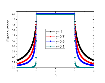
Figure 1: (color online) The Euler number $\chi=2$ in the topological nontrivial phase $\left|h\right|<1$, and ill-defined in the topological trivial phase $\left|h\right|>1$.

Despite the isolated singular points ${k=0,\pm\pi}$ (which is independent on the Hamiltonian parameter $h,\gamma$), it is easy to find from the Eq. (13) that if the parameter $\left|h\right|>1$, then the quantum metric must be degenerate in some region of the Brillouin zone where $1+hk=0$. According to the Theorem 2, it can be understood intuitively as follows: if $\left|h\right|>1,$ then the monopole (anti-monopole) is not enclosed by the surface $\vec{d}(k,\varphi)$. This means that the Berry curvature as a solid angle to the monopole can continuously tend to zero in some region of the Brillouin zone, and then leads to a degenerate quantum metric $\det g_{k\varphi}\left(h,\gamma\right)=0$.

Finally, we illustrate why the surface of the unit vector $\vec{d}(k,\varphi)/d(k,\varphi)$ is unclosed when the parameter $\left|h\right|>1$. The reason is straightforward that: if the parameter $\left|h\right|>1$, then the monopole (coordinate origin) will be not enclosed by the surface $\vec{d}(k,\varphi)$ (see Fig. 2$b$). Hence, if we use the unit vector $\vec{d}(k,\varphi)/d(k,\varphi)$, then the normalized operation $\vec{d}(k,\varphi)/d(k,\varphi)$ will squashed the two surfaces (on the same side of the monopole) flat and make it exhibit a boundary (see Fig. 2$d$).

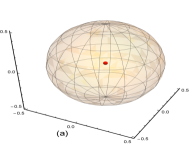
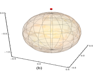
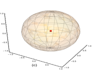
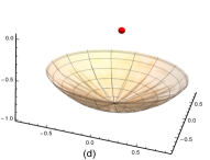
Figure 2: (color online) The trajectories of the vector $\vec{d}\left(k,\varphi\right)$ with the Hamiltonian parameters: (a) $h=0,\gamma=1$, (b) $h=1.2,\gamma=1$; The trajectories of the unit vector $\vec{d}\left(k,\varphi\right)/d\left(k,\varphi\right)$ with the Hamiltonian parameters: (c) $h=0,\gamma=1$, (d) $h=1.2,\gamma=1$. The position of the monopole (coordinates origin) is marked by a red ball.

III.2 Haldane model

The Haldane model Hamiltonian can be expressed in the two-component representation $\left(c_{\mathbf{k}A}^{\dagger},c_{\mathbf{k}B}^{\dagger}\right)$ associated with sublattices A and B as $\mathcal{H}(\mathbf{k})=\epsilon\left(\mathbf{k}\right)\mathbb{I}+\sum_{\alpha=1}^{3}d_{\alpha}\left(\mathbf{k}\right)\sigma^{\alpha}$. Choosing the proper reciprocal lattice vectors, we have

$$\epsilon\left(\mathbf{k}\right) = 2t_{2}\cos\varphi\left[\cos(k_{x})+\cos(k_{y})-\cos(k_{x}+k_{y})\right],$$

$$d_{1}\left(\mathbf{k}\right) = t_{1}\left[\begin{array}[]{c}\cos\left(2k_{x}/3+k_{y}/3\right)+\cos\left(k_{x}/3+2k_{y}/3\right)\\ +\cos\left(k_{x}/3-k_{y}/3\right)\end{array}\right],$$ (20)

$$d_{2}\left(\mathbf{k}\right) = t_{1}\left[\begin{array}[]{c}\sin\left(2k_{x}/3+k_{y}/3\right)-\sin\left(k_{x}/3+2k_{y}/3\right)\\ -\sin\left(k_{x}/3-k_{y}/3\right)\end{array}\right],$$ (23)

$$d_{3}\left(\mathbf{k}\right) = t_{0}-2t_{2}\sin\varphi\left[\begin{array}[]{c}\sin(k_{x})+\sin(k_{y})\\ -\sin(k_{x}+k_{y})\end{array}\right].$$ (26)

According to the Theorem 2, we can use the Berry curvature of the energy band as a tool to determine whether the metric is a proper Riemann metric note2 .

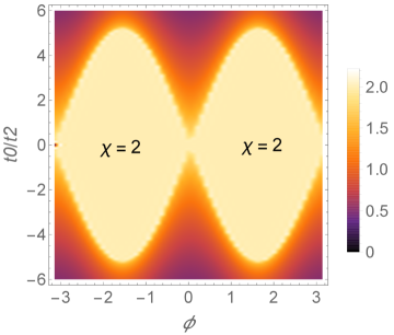
Figure 3: (color online) The phase diagram of Haldane model marked by Euler number of the energy band. The Euler number $\chi=2$ in the topological nontrivial phase $C_{1}=\pm 1$, and is ill-defined in the topological trivial phase $C_{1}=0,$ where the quantum metric is degenerate and its inverse does not exist.

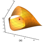
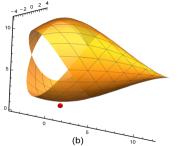
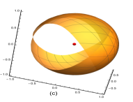
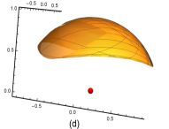
Figure 4: (color online) The trajectories of the vector $\vec{d}\left(\mathbf{k}\right)$ with the Hamiltonian parameters: (a) $t_{0}=0,t_{1}=4,t_{2}=1,\varphi=\pi/2;$ (b) $t_{0}=3\sqrt{3+1},t_{1}=4,t_{2}=1,\varphi=\pi/2;$ The trajectories of the unit vector $\vec{d}\left(\mathbf{k}\right)/d\left(\mathbf{k}\right)$ with the Hamiltonian parameters: (c) $t_{0}=0,t_{1}=4,t_{2}=1,\varphi=\pi/2;$ (d) $t_{0}=3\sqrt{3+1},t_{1}=4,t_{2}=1,\varphi=\pi/2.$ The position of the monopole (coordinates origin) is marked by a red ball.

As shown in the Fig. 3, we find that the Euler number of the filled band is $\chi=2$ corresponding to the Chern number $C_{1}=\pm 1$, and $\chi=$ “non-integer” corresponding to the $C_{1}=0$. It is worth pointing out that the surface of $\vec{d}(\mathbf{k})/d(\mathbf{k})$ for the Haldane Hamiltonian are all unclosed no matter in the topological nontrivial phase or in the trivial phase. It can be seen that, in the topological nontrivial phase, the Euler number for the surface $\vec{d}(\mathbf{k})/d(\mathbf{k})$ itself should be zero due to two boundaries existing on its surface (see Fig. 4$a$ or 4$c$), which makes it topological equivalent to the $S^{1}$ with the Euler number $\chi=0$. However, this is contradictory to the Euler number $\chi=2$ of the occupied band through the Gauss-Bonnet theorem in the topological nontrivial phase. This shows that there is no correspondence between the Euler number of the Bloch band and the Euler number of the $\vec{d}(\mathbf{k})/d(\mathbf{k})$ surface itself.

In addition, as shown in Fig. 4$d$, it is not surprised to find that the normalized operation $\vec{d}(\mathbf{k})/d(\mathbf{k})$ will squashed the two surfaces (on the same side of the monopole) flat and make it exhibit a boundary. The role of the mapping $\vec{d}(\mathbf{k})/d(\mathbf{k})$ unit sphere $S^{2}$ is actually to serve as a states space $\mathcal{C}P^{1}$ for the Fubini-Study metric, but not a parameter manifold for it. However, the quantum metric is defined on a parameter manifold, and the former is only a special case of the quantum metric.

IV Conclusions

In summary, we point out that a well-defined Euler number of the energy band requires a positive definite quantum metric over the first Brillouin zone. We also provide a sufficient criterion for a positive definite quantum metric in a two-dimensional multi-band system based on the corresponding Berry curvature. Furthermore, we show that this criterion is sufficient and necessary in the two-band case. On the other hand, it should be noted that a topological phase characterized by a nontrivial Chern number can not yet ensure the Berry curvature is non-vanishing in the whole Brillouin zone, and hence, a well-defined Euler number of the energy band requires more stronger conditions than a nontrivial Chern number.

It is also interesting to note that the Euler number brings a topological explanation to the notion of the band’s “complexity”, which is introduced by Marzari and Vanderbilt to measure the variation of the band projection operator throughout the Brillouin zone MV . The “complexity” is defined by a gauge invariant Brillouin zone area measured by the quantum metric $\int_{\text{Bz}}d\mathbf{k}\det^{1/2}g\left(\mathbf{k}\right)$. As we now know, this quantity may be a topological number, which differs from the Euler number of the band $\chi=\left(2\pi\right)^{-1}\int_{\text{Bz}}\mathcal{K}dA$ only a constant coefficient if the Berry curvature is non-vanishing in the whole two-dimensional Brillouin zone.

V Acknowledgments

The author thanks Shi-Liang Zhu and Peng Liu for helpful discussions. This work was supported by the NSF of Beijing under Grant No. 1173011, the Scientific Research Project of Beijing Municipal Education Commission (BMEC) under Grant No. KM201711232019, and the Qin Xin Talents Cultivation Program of Beijing Information Science and Technology University (BISTU) under Grant No. QXTCP C201711.

References

- (1) X. Tan, D.-W. Zhang, Z. Yang, J. Chu, Y.-Q. Zhu, D. Li, X. Yang, S. Song, Z. Han, Z. Li, Y. Dong, H.-F. Yu, H. Yan, S.-L. Zhu, and Y. Yu, Phys. Rev. Lett. 122, 210401 (2019).
- (2) Y. Q. Ma, S. J. Gu, S. Chen, H. Fan, and W. M. Liu, arXiv:1202.2397; EPL 103, 10008 (2013).
- (3) Yan-Qing Zhu et al., arXiv:1908.06462; the erratum of Phys. Rev. Lett. 122, 210401 (2019).
- (4) D. Chruscinski and A. Jamiolkowski, Geometric phases in classical and quantum mechanics (Vol. 36) (Springer Science & Business Media, 2012).
- (5) A. T. Rezakhani, D. F. Abasto, D. A. Lidar, and P. Zanardi, Phys. Rev. A 82, 012321 (2010).
- (6) Y. Q. Ma, S. Chen, H. Fan, and W. M. Liu, Phys. Rev. B 81, 245129 (2010).
- (7) Here we can see and are all independent on the , and this can be explained by the following reasons: This model is derived from a one-dimensional BDI class model , with , , , by the following gauge transformation with . Obviously, both and must be independent on the parameter owing to their gauge invariance. On the other hand, we have due to the time-reversal symmetry of , which leads to a vanishing Chern number and fails to characterize the topological charge by using Chern number of the band.
-
(8)
The Berry curvature of the lower occupied band in the
Haldane model is given by , where
- (9) N. Marzari and D. Vanderbilt, Phys. Rev. B 56, 12847 (1997).