Pseudo-Goldstone Dark Matter
in gauged $B-L$ extended Standard Model

Nobuchika Okada, Digesh Raut, and Qaisar Shafi

¹ Department of Physics and Astronomy,
University of Alabama, Tuscaloosa, Alabama 35487, USA
^2,3 Bartol Research Institute, Department of Physics and Astronomy,
University of Delaware, Newark DE 19716, USA

Gauging the global $B-L$ (Baryon number minus Lepton number) symmetry in the Standard Model (SM) is well-motivated since anomaly cancellations require the introduction of three right-handed neutrinos (RHNs) which play an essential role in naturally generating tiny SM neutrino masses through the seesaw mechanism. In the context of the $B-L$ extended SM, we propose a pseudo-Goldstone boson dark matter (DM) scenario in which the imaginary component of a complex $B-L$ Higgs field serves as the DM in the universe. The DM relic density is determined by the SM Higgs boson mediated process, but its elastic scattering with nucleons through the exchange of Higgs bosons is highly suppressed due to its pseudo-Goldstone boson nature. The model is therefore free from the constraints arising from direct DM detection experiments. We identify regions of the model parameter space for reproducing the observed DM density compatible with the constraints from the Large Hadron Collider and the indirect DM searches by Fermi-LAT and MAGIC.

1 Introduction

According to the widely accepted $\Lambda_{CDM}$ model [1] around 25% of the universe’s total energy density resides in one or more dark matter (DM) particle. A neutral weakly interacting massive particle (WIMP), incorporated in new physics beyond the Standard Model (SM), remains an attractive DM candidate. The so-called Higgs-portal scalar DM [2] is a well-studied WIMP DM scenario, in which a SM singlet real scalar field plays the role of WIMP DM through its renormalizable interaction with the SM Higgs boson. Because of its simplicity, the physics of the Higgs-portal scalar DM scenario is determined by only two parameters, a quartic coupling between the scalar DM and the SM Higgs doublet ($\lambda_{HSS}$) and the DM mass ($m_{S}$). The constraint from the observed DM relic density determines $\lambda_{HSS}$ as a function of $m_{S}$, in which case the latter is the unique free parameter of the scenario.

A number of DM detection experiments have been searching for a signal from a DM particle scattering off nuclei. No evidence for this has so far been observed, and the most stringent upper bound is reported by XENON1T experiment [3] and the DarkSide-50 experiment [4] for a DM mass $m_{S}[{\rm GeV}]>6$ and $1\leq m_{S}[{\rm GeV}]\leq 6$, respectively. For the Higgs-portal scalar DM, the upper bound on DM-nucleon scattering cross section leads to a lower bound on $\lambda_{HSS}$. For $1\,{\rm GeV}<m_{S}\lesssim$ a few TeV, almost the entire region which can reproduce the observed DM density with $\lambda_{HSS}$ in perturbative regime is excluded, except for a very narrow region in the vicinity of the Higgs boson resonance point of $m_{S}\simeq m_{h}/2\simeq 62.5$ GeV. Studies of the Higgs boson decay at the Large Hadron Collider (LHC) [5] exclude the region $m_{S}<1$ GeV, which predicts a large invisible branching ratio into a pair of DM particles. Although the Higgs-portal scalar DM scenario is relatively straightforward scenario, only a very limited parameter region is allowed. See Ref. [6] for a review on the current status of the Higgs-portal DM scenario.

Recently, a so-called pseudo-Goldstone DM (pGDM) model has been proposed in Ref. [7], which is an extension of the Higgs-portal scalar DM scenario with a (broken) global U(1) symmetry. The basic idea is the following: It contains a single complex scalar $S$ and its mass term takes the form

$$\mu_{S}^{2}\left(S^{2}+(S^{\dagger})^{2}\right),$$ (1.1)

where $\mu_{S}$ is a real mass parameter. In the absence of this term, the model possesses a global U(1) symmetry, which is broken by a nonzero vacuum expectation value (VEV) of the real part of $S$. The imaginary component of $S$ (we call it $\chi$) is a massless Nambu-Goldstone (NG) particle in the limit $\mu_{S}\to 0$. Even for $\mu_{S}\neq 0$, the model has a $Z_{2}$ symmetry under which $\chi$ has an odd-parity and all the other fields including the SM fields are even. Hence, $\chi$ is stable and a Higgs-portal scalar DM candidate. A characteristic feature of this model is that despite $\mu_{S}\neq 0$, $\chi$ retains a Goldstone boson nature with a derivative coupling to the Higgs boson. As a result, this coupling disappears in the non-relativistic limit, so that the scattering cross section of the DM particle $\chi$ with a nucleon mediated by the Higgs bosons vanishes [7]. This model is therefore free from the constraints from the direct DM detection experiments.

In this paper we propose a pGDM model based on a simple extension of the minimal $B-L$ (Baryon number minus Lepton number) model [8], where the anomaly-free global $B-L$ symmetry of the SM is gauged. We introduce an additional scalar field relative to the minimal $B-L$ model which has a unit $B-L$ charge and whose imaginary component pays the role of pGDM. Except for the DM physics, the phenomenology of the model is much the same as that of the minimal $B-L$ model. The gauge and mixed gauge-gravitational anomalies are all canceled by the presence of three right-handed neutrinos (RHNs), which acquire their Majorana masses associated with $B-L$ symmetry breaking. With the Majorana RHNs and electroweak symmetry breaking, the seesaw mechanism works to generate the tiny neutrino masses. The model can also account for the observed baryon asymmetry of the universe through leptogenesis [9].

Our gauge extension of the pGDM model has another theoretical advantage. In the original pGDM model [7], in order to realize a phenomenologically viable scenario it is essential to introduce the mass squared terms in Eq. (1.1) which explicitly break the global U(1) symmetry. Since the latter symmetry is not manifest one could, in general, include additional terms. However, with such general terms, the DM particle looses its Goldstone boson nature and the model will be severely constrained by the direct DM detection experiments. As we discuss in the next section, we effectively realize the terms in Eq. (1.1) after $B-L$ symmetry breaking, and any unwanted terms is forbidden by the $B-L$ symmetry. Therefore, we may consider our model as an ultraviolet completion of the original pGDM model.

Unlike the original model in Ref. [7] where a $Z_{2}$ symmetry ensures the stability of the DM particle, the $B-L$ gauge interaction explicitly violates this parity, and hence the DM particle is not entirely stable. This fact implies a lower bound on the $B-L$ symmetry breaking scale in order to yield a sufficiently long-lived DM particle. Although the pGDM evades the direct detection constraints, we examine constraints on the model parameter space from the LHC and from indirect DM search experiments, such as the Fermi Large Area Telescope (Fermi-LAT) [10] and Major Atmospheric Gamma Imaging Cherenkov Telescopes (MAGIC) [11]. See also Ref. [12].

This paper is organized as follows: In Sec. 2 we present our pGDM model in the $B-L$ framework. We first describe the basic structure of the model, and then show that the DM-nucleon scattering amplitude vanishes in the non-relativistic limit. We also estimate the lifetime of the pGDM and obtain a lower bound on the $B-L$ symmetry breaking scale. In Sec. 3 we identify the parameter region compatible with the observed DM relic density. In Sec. 4 we constrain the parameter space of our model by taking into account LHC and indirect DM search experiments. Our conclusions are summarized in Sec. 5.

2 pGDM in $B-L$ extended Standard Model

	SU(3)c	SU(2)L	U(1)Y	U(1)B-L
$q^{i}_{L}$	3	2	$1/6$	$1/3$
$u^{i}_{R}$	3	1	$2/3$	$1/3$
$d^{i}_{R}$	3	1	$-1/3$	$1/3$
$\ell^{i}_{L}$	1	2	$-1/2$	$-1$
$e^{i}_{R}$	1	1	$-1$	$-1$
$H$	1	2	$-1/2$	$0$
$N^{i}_{R}$	1	1	$0$	$-1$
$\Phi_{A}$	1	1	$0$	$+2$
$\Phi_{B}$	1	1	$0$	$-1$

Table 1: The particle content of our $B-L$ extended SM. In addition to the SM particle content ($i=1,2,3$), we have three RHNs ($N_{R}^{i}$) and two $B-L$ Higgs fields ($\Phi_{A,B}$). The model reduces to the minimal $B-L$ model if we omit $\Phi_{B}$.

We consider a $B-L$ extension of the SM that incorporates a pGDM particle. The field content is listed in Table 1. In addition to the SM fields, the model includes three right-handed neutrinos ($N_{R}^{i}$) in order to cancel all the gauge and mixed gauge-gravitational anomalies. The scalar sector includes two new SM singlet Higgs fields, $\Phi_{A}$ and $\Phi_{B}$, with $B-L$ charges $+2$ and $-1$, respectively. This charge assignment for $\Phi_{A,B}$ is crucial for incorporating a pGDM particle. Note that the model reduces to the minimal $B-L$ model if we omit the new Higgs field $\Phi_{B}$.

The SM Yukawa sector for the RHNs is extended to include in the Lagrangian density the following terms,

$${\cal L}\supset-\frac{1}{2}\sum_{i,j=1}^{3}Y_{D}^{ij}{\overline{\ell}^{i}}HN_{R}^{j}-\frac{1}{2}\sum_{i=1}^{3}Y_{N}^{i}\Phi_{A}\overline{N_{R}^{i~{}C}}N^{i}_{R}+{\rm h.c.},$$ (2.1)

where we have assumed a diagonal basis for the Majorana Yukawa couplings. After the electroweak and $B-L$ symmetry breaking, the Dirac and the Majorana masses for the RHNs are generated,

$$m_{D}^{ij}=\frac{Y_{D}^{ij}}{\sqrt{2}}v_{H},\;\;m_{N^{i}}=\frac{1}{\sqrt{2}}Y_{N}^{i}v_{A},$$ (2.2)

where $v_{H}=\sqrt{2}\langle H^{0}\rangle=246$ GeV is a VEV of the charge neutral component ($H^{0}$) of the SM Higgs doublet, and $v_{A}=\sqrt{2}\langle\Phi_{A}\rangle$.

2.1 Realizing pGDM

Let us consider the scalar sector of the model. The gauge invariant and renormalizable scalar potential for $\Phi_{A,B}$ and $H$ is given by

$$V= - \mu_{H}^{2}\left(H^{\dagger}H\right)-\mu_{A}^{2}\left(\Phi_{A}^{\dagger}\Phi_{A}\right)-\mu_{B}^{2}\left(\Phi_{B}^{\dagger}\Phi_{B}\right)$$ (2.3)

$$+ \lambda_{H}\left(H^{\dagger}H\right)^{2}+\lambda_{HA}\left(H^{\dagger}H\right)\left(\Phi_{A}^{\dagger}\Phi_{A}\right)+\lambda_{HB}\left(H^{\dagger}H\right)\left(\Phi_{B}^{\dagger}\Phi_{B}\right)$$

$$+ \lambda_{AB}\left(\Phi_{A}^{\dagger}\Phi_{A}\right)\left(\Phi_{B}^{\dagger}\Phi_{B}\right)+\lambda_{A}\left(\Phi_{A}^{\dagger}\Phi_{A}\right)^{2}+\lambda_{B}\left(\Phi_{B}^{\dagger}\Phi_{B}\right)^{2}$$

$$- \sqrt{2}\Lambda\left(\Phi_{A}\,\Phi_{B}^{2}+{\text{h.c}}\right),$$

where $\mu_{A,B,H}$ , $\Lambda$, and quartic scalar coupling parameters ($\lambda_{i}$) are all real parameters with mass dimension $2,1$, and $0$, respectively. This scalar potential is invariant under transformation $\Phi_{A,B}\to\Phi_{A,B}^{\dagger}$. This indicates that the real components of $\Phi_{A,B}$ are ${Z}_{2}$-even (${\rm Re}[\Phi_{A,B}]\to{\rm Re}[\Phi_{A,B}]$), while their imaginary components are ${Z}_{2}$-odd (${\rm Im}[\Phi_{A,B}]\to-{\rm Im}[\Phi_{A,B}]$). Arranging suitably the parameters in the scalar potential, we obtain the $B-L$ symmetry breaking by $\langle{\rm Re}[\Phi_{A,B}]\rangle\neq 0$. After this breaking, a linear combination of ${\rm Im}[\Phi_{A}]$ and ${\rm Im}[\Phi_{B}]$ forms the would-be Nambu-Goldstone (NG) mode which is eaten by the the $B-L$ gauge boson ($Z^{\prime}$). Its orthogonal combination is a physical massive scalar which, as we will see below, is the desired pGDM particle. Note that the covariant derivatives for $\Phi_{A,B}$ explicitly break the symmetry $\Phi_{A,B}\to\Phi_{A,B}^{\dagger}$ and so the pGDM is not stable. We will discuss its lifetime later.

Let us first consider the mass spectrum of the model. We express the scalar fields as

$$\Phi_{A,B} = \frac{1}{\sqrt{2}}\left(\phi_{A,B}+v_{A,B}+i\chi_{A,B}\right)$$

$$H^{0} = \frac{1}{\sqrt{2}}\left(h+v_{H}\right),$$ (2.4)

where $v_{B}=\sqrt{2}\langle\Phi_{B}\rangle$. The stationary conditions around the VEVs lead to

$$\mu_{A}^{2} = \lambda_{A}v_{A}^{2}-\frac{\Lambda v_{B}^{2}}{v_{A}}+\frac{1}{2}\lambda_{AB}v_{B}^{2}+\frac{1}{2}\lambda_{HA}v_{H}^{2},$$

$$\mu_{B}^{2} = \frac{1}{2}\left(\lambda_{AB}v_{A}^{2}-4\Lambda v_{A}+2\lambda_{B}v_{B}^{2}+\lambda_{HB}v_{H}^{2}\right),$$

$$\mu_{H}^{2} = \frac{1}{2}\left(2\lambda_{H}v_{H}^{2}+\lambda_{HA}v_{A}^{2}+\lambda_{HB}v_{B}^{2}\right).$$ (2.5)

Substituting Eqs. (2.4) and (2.5) into Eq. (2.3), we obtain the mass matrices for the real and imaginary components, respectively. Since the $Z_{2}$ symmetry is manifest for the scalar potential, there is no mixing between the real and imaginary components. For the real components, the mass matrix is given by

$$V\supset\frac{1}{2}\begin{bmatrix}\phi_{A}&\phi_{B}&h\end{bmatrix}\begin{bmatrix}\Lambda\frac{v_{B}^{2}}{v_{A}}+2\lambda_{A}v_{A}^{2}&v_{B}\left(-2\Lambda+v_{A}\lambda_{AB}\right)&\lambda_{HA}v_{A}v_{H}\\ v_{B}\left(-2\Lambda+v_{A}\lambda_{AB}\right)&2\lambda_{B}v_{B}^{2}&\lambda_{HB}v_{B}v_{H}\\ \lambda_{HA}v_{A}v_{H}&\lambda_{HB}v_{B}v_{H}&2\lambda_{H}v_{H}^{2}\end{bmatrix}\begin{bmatrix}\phi_{A}\\ \phi_{B}\\ h\end{bmatrix},$$ (2.6)

and the corresponding imaginary component mass matrix is given by

$$V\supset\frac{1}{2}\begin{bmatrix}\chi_{A}&\chi_{B}\end{bmatrix}\begin{bmatrix}\Lambda\frac{v_{B}^{2}}{v_{A}}&2\Lambda v_{B}\\ 2\Lambda v_{B}&4\Lambda v_{A}\end{bmatrix}\begin{bmatrix}\chi_{A}\\ \chi_{B}\end{bmatrix}.$$ (2.7)

We first diagonalize the mass matrix for the imaginary components,

$$\begin{bmatrix}\chi_{A}\\ \chi_{B}\end{bmatrix}=\begin{bmatrix}-\cos\theta&\sin\theta\\ \sin\theta&\cos\theta\end{bmatrix}\begin{bmatrix}{\chi_{1}}\\ {\chi_{2}}\end{bmatrix},$$ (2.8)

where $\chi_{1,2}$ are the mass eigenstates, and

$$\sin\theta=\frac{v_{B}}{\sqrt{4v_{A}^{2}+v_{B}^{2}}}\;,\qquad\cos\theta=\frac{2v_{A}}{\sqrt{4v_{A}^{2}+v_{B}^{2}}}.$$ (2.9)

The mass eigenvalues of $\chi_{1,2}$ are given by

$$m_{1}^{2} = 0,$$

$$m_{2}^{2} = 4\Lambda v_{A}\left(1+\tan^{2}\theta\right).$$ (2.10)

In the following, we employ the $R_{\xi}$-gauge to show that $\chi_{1}$ is the would-be NG mode absorbed by the gauge boson $Z^{\prime}$, and $\chi_{2}$ is the pGDM. The kinetic terms for the scalars and the gauge field are given by

$${\mathcal{L}}\supset\left(D^{A}_{\mu}\Phi_{A}\right)^{\dagger}\left(D^{A\mu}\Phi_{A}\right)+\left(D^{B}_{\mu}\Phi_{B}\right)^{\dagger}\left(D^{B\mu}\Phi_{B}\right)-{\cal Z}^{\prime}_{\mu\nu}{\cal Z}^{\prime\mu\nu}-\frac{1}{2\xi}\left(\partial_{\mu}{Z^{\prime}}^{\mu}+\xi\gamma\chi_{1}\right)^{2}.$$ (2.11)

Here, $D^{A,B}_{\mu}={\partial}_{u}-igQ_{A,B}Z^{\prime}_{\mu}$ is the covariant derivative for $\Phi_{A,B}$ with $Q_{A}=+2$ and $Q_{B}=-1$, respectively, ${\cal Z}^{\prime}_{\mu\nu}$ is the $Z^{\prime}$ boson field strength, $\xi$ is the gauge fixing parameter, and $\gamma=g(2v_{A}\cos\theta+v_{B}\sin\theta)=g\sqrt{4v_{A}^{2}+v_{B}^{2}}$. The choice of $\gamma$ eliminates the mixing terms $\chi_{1,2}(\partial^{\mu}Z^{\prime})$. We rewrite Eq. (2.11) in terms of the mass eigenstates as

$${\cal L} \supset \frac{1}{2}{Z^{\prime}}^{\mu}\left(\eta_{\mu\nu}\partial_{\alpha}\partial^{\alpha}-\left(1-\frac{1}{\xi}\right)\partial_{\mu}\partial_{\nu}\right){Z^{\prime}}^{\nu}+\frac{1}{2}\gamma^{2}{Z^{\prime}}_{\mu}{Z^{\prime}}^{\mu}$$ (2.12)

$$+ \frac{1}{2}\left(\partial_{\mu}\chi_{1}\right)\left(\partial^{\mu}\chi_{1}\right)-\frac{1}{2}\xi\gamma^{2}\chi_{1}^{2}+\frac{1}{2}\left(\partial_{\mu}\chi_{2}\right)\left(\partial^{\mu}\chi_{2}\right)-\frac{1}{2}m_{2}^{2}\chi_{2}^{2}$$

$$- 2g\left(-2\sin\theta\phi_{A}+\cos\theta\phi_{B}\right)\left(\partial_{\mu}\chi_{2}\right){Z^{\prime}}^{\mu}.$$

Here, as usual in $R_{\xi}$-gauge, $\gamma$ is identified with the $B-L$ gauge boson mass, $\gamma=m_{Z^{\prime}}$, and $\chi_{1}$ is the would-be NG mode whose mass squared is given by $\xi m_{Z^{\prime}}^{2}$. In the following, we employ the unitary gauge ($\xi\to\infty$), such that the would-be NG mode $\chi_{1}$ decouples from the system. The last line of Eq. (2.12) shows that the ${Z_{2}}$ parity is not manifest in the gauge sector, and $\chi_{2}$ decays through this triple coupling. In the next subsection, we estimate the lifetime of $\chi_{2}$. As expected, if $Z^{\prime}$ and $\phi_{A,B}$ are sufficiently heavy, $\chi_{2}$ can be sufficiently long-lived in order to be a viable DM in the universe.

2.2 pGDM Direct Detection Amplitude and Lifetime

To check if the elastic scattering cross section of the pGDM ($\chi_{2}$) with nucleons is adequately suppressed and its lifetime is long enough, let us first consider the so-called “spurion” limit. In this limit, we take $v_{A}\gg v_{B},v_{H}$, $\lambda_{A}v_{A}^{2}\gg\Lambda v_{B}$, and $\lambda_{AH},\lambda_{AB}\to 0$, so that the mass matrix of Eq. (2.6) becomes block-diagonal and $\phi_{A}$ is decoupled from the system. We have $\theta\ll 1$ in Eq. (2.8) for $v_{A}\gg v_{B}$, and thus $\chi_{1}\simeq-\chi_{A}$ and the pGDM $\chi_{2}\simeq\chi_{B}$. Therefore, in the spurion limit (and in the unitary gauge), $\Phi_{A}$ looses its dynamical degrees of freedom and works as an external field with $\langle\Phi_{A}\rangle$. Next, we consider the following mass matrix for $\phi_{B}$ and $h$:

$$V\supset\frac{1}{2}\begin{bmatrix}\phi_{B}&h\end{bmatrix}\begin{bmatrix}2\lambda_{B}v_{B}^{2}&\lambda_{HB}v_{B}v_{H}\\ \lambda_{HB}v_{B}v_{H}&2\lambda_{H}v_{H}^{2}\end{bmatrix}\begin{bmatrix}\phi_{B}\\ h\end{bmatrix}.$$ (2.13)

If we ignore the $B-L$ gauge interaction, the spurion limit effectively realizes the original pGDM model.

The elastic scattering of pGDM ($\chi_{B}$) with nucleons is mediated by two Higgs bosons which are linear combinations of $h$ and $\phi_{B}$. The amplitude of the scattering is readily evaluated in the flavor basis. The relevant terms for this analysis are given by

$${\cal L}\supset S^{\dagger}(\Box+M_{S})S+C_{SBB}S\chi_{B}^{2}+C_{hff}S{\bar{f}}_{SM}f_{SM},$$ (2.14)

where $S\equiv(\phi_{B},h)^{\rm T}$, $M_{S}$ is the $2\times 2$ mass matrix defined in Eq. (2.13), $C_{SBB}=(\lambda_{B}v_{B},\lambda_{BH}v_{H}/2)$, and the last term is the Yukawa interaction of $h$ with SM fermions with $C_{hff}=Y_{hf{\bar{f}}}(0,1)$. Now we can express the scattering amplitude as

$${\cal M}\propto C_{BBS}\;\frac{1}{t-M_{S}}\;C_{hff}^{\rm T}.$$ (2.15)

Since this scattering occurs at very low energies, the zero momentum transfer limit of $t\to 0$ is a good approximation:

$${\cal M}(t\to 0) \propto C_{BBh}\;M_{S}^{-1}\;C_{hff}^{\rm T},$$ (2.16)

$$\propto \begin{bmatrix}\lambda_{B}v_{B}&\lambda_{HB}v_{H}/2\end{bmatrix}\begin{bmatrix}2\lambda_{H}v_{H}^{2}&-\lambda_{HB}v_{B}v_{H}\\ -\lambda_{HB}v_{B}v_{H}&2\lambda_{B}v_{B}^{2}\end{bmatrix}\begin{bmatrix}0\\ 1\end{bmatrix}=0.$$

Therefore, the pGDM scattering amplitude vanishes in the $t\to 0$ limit.

Before moving on to a more general analysis for the pGDM scattering amplitude by taking $\phi_{A}$ into account, let us estimate the pGDM lifetime in the spurion limit. The pGDM decays through the interaction,

$${\cal L}\supset-2g\phi_{B}\left(\partial_{\mu}\chi_{B}\right)Z^{\prime\mu}.$$ (2.17)

As an example, we consider a pGDM mass of $m_{DM}\sim 100$ GeV. Since both the $Z^{\prime}$ boson and $\phi_{B}$ have couplings with SM fermions (the latter through its mixing with the SM Higgs boson), the main decay mode is $\chi_{B}\to{Z^{\prime}}^{*}\phi_{B}^{*}\to{\bar{f}}_{SM}f_{SM}{\bar{f}}_{SM}f_{SM}$ through off-shell $\phi_{B}$ and $Z^{\prime}$, where $f_{SM}$ represents a SM fermion. We estimate the pGDM lifetime to be

$$\tau_{DM}\simeq\frac{(10\pi)^{5}}{Y_{b}^{2}\sin^{2}\theta_{H}}\left(\frac{v_{A}}{m_{DM}}\right)^{4}\left(\frac{m_{B}}{m_{DM}}\right)^{4}(m_{DM})^{-1},$$ (2.18)

where $Y_{b}$ is the bottom Yukawa coupling, $m_{B}$ is the mass of $\phi_{B}$, and $\sin\theta_{H}$ quantifies the mixing of $\phi_{B}$ with the SM Higgs boson. If we require a lower bound $\tau_{DM}\gtrsim 10^{26}$ sec from the cosmic ray observations [15], we find

$$v_{A}\gtrsim 1.22\times 10^{11}{\rm GeV}\left(\frac{600\;{\rm GeV}}{m_{B}}\right)\left(\frac{m_{DM}}{100\;{\rm GeV}}\right)^{9/4}\left(\frac{\sin\theta_{H}}{0.2}\right)^{1/2}.$$ (2.19)

The stability of the DM particle requires $v_{A}$ to be at the intermediate scale or higher. In our model, we assume a vanishing kinetic mixing between $Z^{\prime}$ and the SM $Z$ bosons. If the mixing which we parametrize as $\epsilon$ exists, the DM particle has an interaction with $Z$ boson given by Eq. (2.17) with a replacement $Z^{\prime\mu}\to\epsilon Z^{\mu}$. Considering the decay mode of $\chi_{B}\to Z^{*}\phi_{B}^{*}\to{\bar{f}}_{SM}f_{SM}{\bar{f}}_{SM}f_{SM}$, we find an upper bound $\epsilon\lesssim(v_{H}/v_{A})^{2}={\cal O}(10^{-18})$ for $v_{A}={\cal O}(10^{11})$ GeV.

Let us now calculate the pGDM scattering amplitude for the more general case by taking $\phi_{A}$ into account. In this case, the pGDM is a linear combination of $\chi_{A}$ and $\chi_{B}$ as defined in Eq. (2.8), and the pGDM scattering with a nucleon is mediated by three Higgs mass eigenstates which are linear combinations of $h$, $\phi_{A}$ and $\phi_{B}$. Because of the presence of the extra scalar $\phi_{A}$, the vanishing scattering amplitude for the limit of $t\to 0$ is not guaranteed. We work in the flavor basis with $S=(\phi_{A},\phi_{B},h)^{\rm T}$, and the relevant terms are given by

$${\cal L}\supset S^{\dagger}(\Box+M_{S})S+C_{hff}S{\bar{f}}_{SM}f_{SM}+\left(C_{AAS}S+C_{BBS}S+C_{ABS}S\right)\chi_{2}^{2}.$$ (2.20)

Here, $M_{S}$ is the $3\times 3$ mass matrix in Eq. (2.6), the second term is the interaction of $h$ with the SM fermions $C_{hff}=Y_{hf\bar{f}}\,(0,0,1)$, and

$$C_{AAS} = \sin^{2}\theta\left(2\lambda_{A}v_{A},\;\lambda_{AB}v_{B},\;\lambda_{HA}v_{H}\right),$$

$$C_{BBS} = \cos^{2}\theta\left(2\Lambda+\lambda_{AB}v_{A},\;2\lambda_{B}v_{B},\;\lambda_{HB}v_{H}\right),$$

$$C_{ABS} = \sin\theta\cos\theta\left(0,\;2\Lambda,\;0\right).$$ (2.21)

The total amplitude in the limit of $t\to 0$ is expressed as

$${\cal M}\propto\left(C_{AAS}+C_{BBS}+C_{ABS}\right)\;M_{S}^{-1}\;C_{hff}^{\rm T}.$$ (2.22)

We have previously found that $v_{A}$ must be higher than the intermediate scale in order to make the pGDM sufficiently long-lived. Thus, in order not to significantly alter the SM-like Higgs boson mass eigenvalue from the mass matrix of Eq. (2.6), we set $\lambda_{AH}\to 0$ in the following analysis. The amplitude is then expressed as

$${\cal M}\propto\frac{\Lambda\lambda_{HB}\cos^{2}\theta\left(4\Lambda+v_{A}\left(\lambda_{A}-2\lambda_{AB}\right)+2\tan^{2}\theta\left(\Lambda+v_{A}\left(\lambda_{A}+\lambda_{AB}\tan^{2}\theta\right)\right)\right)}{v_{H}\left(\lambda_{H}\left(\left(\lambda_{AB}^{2}v_{A}-2\Lambda\right)^{2}-4v_{A}^{2}\lambda_{A}\lambda_{B}\right)+v_{A}^{2}\lambda_{A}\lambda_{HB}^{2}+2v_{A}\Lambda\tan^{2}\theta\left(-4\lambda_{B}\lambda_{H}+\lambda_{HB}\right)\right)}.$$ (2.23)

Because of the perturvativity constraint for the Higgs-portal scalar DM scenario, we are interested in a DM mass ($m_{DM}=m_{2}$) less than a few TeV. From Eq. (2.10), we find $\Lambda\sim m_{DM}^{2}/v_{A}\ll 1$. This simplifies the amplitude formula to

$${\cal M}\propto\frac{\Lambda\lambda_{HB}\left(2\lambda_{A}-4\lambda_{AB}\right)}{2v_{A}v_{H}\left(\lambda_{H}\lambda_{AB}^{2}+\lambda_{A}\left(\lambda_{HB}^{2}-4\lambda_{B}\lambda_{H}\right)\right)}\propto\frac{\Lambda}{v_{A}},$$ (2.24)

which is adequately suppressed. To obtain the final expression in Eq. (2.24), we have set all the quartic couplings to be of the same order. Note that ${\mathcal{M}}=0$ cannot be realized even for the momentum transfer $t=0$. This is because the last term in Eq. (2.3), $\Lambda\left(\Phi_{A}\,\Phi_{B}^{2}\right)$, introduces non-derivative coupling between the DM and the scalars and the Goldstone boson nature of the DM particle is lost.

3 DM relic density

In this section we numerically evaluate the thermal relic density of the DM particle by solving the Boltzmann equation,

$$\frac{dY}{dx}=-\frac{\langle\sigma v\rangle}{x^{2}}\frac{s(m_{2})}{H(m_{2})}\left(Y^{2}-Y_{EQ}^{2}\right).$$ (3.1)

Here, $x=m_{2}/T$ is a dimensionless parameter where $T$ is the temperature of the Universe, $H(m_{2})$ is the Hubble parameter and $Y=n/s$ is the DM yield which is defined as the ratio of the DM number density ($n$) to the entropy density ($s$), and $Y_{EQ}$ is the yield of the DM particle in thermal equilibrium:

$$s(m_{2})=\frac{2\pi^{2}}{45}g_{\star}m_{2}^{3},\;\;H(m_{2})=\sqrt{\frac{\pi^{2}}{90}g_{\star}}\frac{m_{2}^{2}}{M_{P}},\;\;Y_{EQ}(x)=\frac{g_{DM}}{2\pi^{2}}\frac{x^{2}m_{2}^{3}}{s(m_{2})}K_{2}(x),$$ (3.2)

where $K_{2}$ is the Bessel function of the second kind. The thermal average of the total pair annihilation cross section of the DM particles times its relative velocity, $\langle\sigma v\rangle$ in Eq. (3.1), can be evaluated as

$$\langle\sigma v\rangle=\frac{g_{DM}^{2}}{64\pi^{4}}\left(\frac{m_{3}}{x}\right)\frac{1}{n_{EQ}^{2}}\int_{4m_{3}^{2}}^{\infty}ds\;2(s-4m_{3}^{2})\sigma(s)\sqrt{s}K_{1}\left(\frac{x\sqrt{s}}{m_{3}}\right),$$ (3.3)

where $g_{DM}(=1)$ counts the degrees of freedom of the scalar DM particle, the equilibrium number density of the DM particle $n_{EQ}=s(m_{2})Y_{EQ}/x^{3}$, $\sigma(s)$ is the total DM particle annihilation cross section, and $K_{1}$ is the modified Bessel function of the first kind. The relic density of the DM particle at the present time is evaluated as

$$\Omega_{DM}h^{2}=\frac{m_{3}s_{0}Y(x\to\infty)}{\rho_{c}/h^{2}},$$ (3.4)

where $s_{0}=2890$ cm^-3 is the entropy density of the present Universe and $\rho_{c}/h^{2}=1.05\times 10^{-5}$ GeV/cm³ is the critical density. The Planck satellite experiment has measured $\Omega_{DM}h^{2}=0.1200\pm 0.0012$ [1].

In the following, we consider the spurion limit case to be our benchmark, namely, $v_{A}\gg v_{B},v_{H}$, $\lambda_{A}v_{A}^{2}\gg\Lambda v_{B}$, and $\lambda_{AH},\lambda_{AB}\to 0$. In this limit $\phi_{A}$ is decoupled from the system and the DM mass eigenstate $\chi_{2}\simeq\chi_{B}$. The real sector includes $\phi_{B}$ and $h$ that mix according to the mass matrix in Eq. (2.13) which we diagonalize by defining the mass eigenstates ${\tilde{\phi}_{B}}$ and ${\tilde{h}}$ as follows:

$$\begin{bmatrix}\phi_{B}\\ h\end{bmatrix}=\begin{bmatrix}\cos\theta_{H}&-\sin\theta_{H}\\ \sin\theta_{H}&\cos\theta_{H}\end{bmatrix}\begin{bmatrix}{\tilde{\phi}_{B}}\\ {\tilde{h}}\end{bmatrix}.$$ (3.5)

Here, the mixing angle $\theta_{H}$ is determined by

$$2v_{B}v_{H}\lambda_{HB}=(m_{B}^{2}-m_{h}^{2})\tan 2\theta_{H}.$$ (3.6)

The masses of ${\tilde{\phi}_{B}}$ and ${\tilde{h}}$ are given by

$${m}_{{\tilde{B}},{\tilde{h}}}^{2}=\frac{1}{2}\left(m_{B}^{2}+m_{h}^{2}\pm\frac{m_{B}^{2}-m_{h}^{2}}{\cos 2\theta_{H}}\right),$$ (3.7)

respectively, where $m_{h}=2\lambda_{h}v_{H}^{2}$. The interaction between the DM and $\tilde{h}$/${\tilde{\phi}}_{B}$ is given by

$${\cal L}\supset\frac{{\lambda_{\tilde{h}}}\;v_{H}}{2}\;{\tilde{h}}\chi_{2}\chi_{2}+\frac{{\lambda_{\tilde{B}}}\;v_{H}}{2}\;{\tilde{\phi}_{B}}\chi_{2}\chi_{2},$$ (3.8)

where

$${\lambda_{\tilde{h}}} = -\frac{2{m}_{{\tilde{h}}}^{2}}{v_{B}v_{H}}\sin\theta_{H},$$

$${\lambda_{\tilde{B}}} = +\frac{2{m}_{{\tilde{B}}}^{2}}{v_{B}v_{H}}\cos\theta_{H}.$$ (3.9)

To evaluate the DM relic density, let us set $m_{B}=600$ GeV and $\sin\theta_{H}=0.2$ to be our benchmark. In this case, for the DM mass $m_{2}\lesssim 200$ GeV, the DM scenario is effectively the same as the Higgs-portal scalar DM scenario such that the DM interaction is given by the first term in Eq. (3.8). The DM pair annihilation processes and therefore the DM relic abundance is determined by only two free parameters, namely, $m_{2}$ and $\lambda_{\tilde{h}}$. The DM pair annihilation processes include various final states that include SM fermions ($f$), the weak gauge bosons ($W$ and $Z$) and the SM Higgs boson ($h$). The DM annihilation cross sections for the various final states are given by [16]:

$${\sigma}_{ff} = \sum_{f}\frac{\lambda_{\tilde{h}}^{2}m_{f}^{2}}{\pi}\frac{1}{(s-m_{{\tilde{h}}}^{2})^{2}+m_{{\tilde{h}}}^{2}\Gamma_{{\tilde{h}}}^{2}}\frac{(s-4m_{f}^{2})^{\frac{3}{2}}}{\sqrt{s}},$$

$${\sigma}_{ZZ} = \frac{\lambda_{\tilde{h}}^{2}}{4\pi}\frac{s^{2}}{(s-m_{{\tilde{h}}}^{2})^{2}+m_{{\tilde{h}}}^{2}\Gamma_{{\tilde{h}}}^{2}}\sqrt{1-\frac{4m_{Z}^{2}}{s}}\left(1-\frac{4m_{Z}^{2}}{s}+\frac{12m_{Z}^{4}}{s^{2}}\right),$$

$${\sigma}_{WW} = \frac{\lambda_{\tilde{h}}^{2}}{2\pi}\frac{s^{2}}{(s-m_{{\tilde{h}}}^{2})^{2}+m_{{\tilde{h}}}^{2}\Gamma_{{\tilde{h}}}^{2}}\sqrt{1-\frac{4m_{W}^{2}}{s}}\left(1-\frac{4m_{W}^{2}}{s}+\frac{12m_{W}^{4}}{s^{2}}\right),$$

$${\sigma}_{{\tilde{h}}{\tilde{h}}} = \frac{\lambda_{\tilde{h}}^{2}}{4\pi}\sqrt{1-\frac{4m_{{\tilde{h}}}^{2}}{s}}\left[\left(\frac{s+2m_{{\tilde{h}}}^{2}}{s-m_{{\tilde{h}}}^{2}}\right)^{2}-\frac{16\lambda_{\tilde{h}}v_{H}^{2}}{s-2m_{{\tilde{h}}}^{2}}\frac{s+2m_{{\tilde{h}}}^{2}}{s-m_{{\tilde{h}}}^{2}}F(\alpha)\right.$$ (3.10)

$$\left.+\frac{32\lambda_{\tilde{h}}^{2}v_{H}^{4}}{(s-2m_{{\tilde{h}}}^{2})^{2}}\left(\frac{1}{1-\alpha^{2}}+F(\alpha)\right)\right],$$

where $m_{h}=125$ GeV is the SM Higgs boson mass, $s$ is the square of the center-of-mass energy, $F(\alpha)\equiv\mbox{arctanh}(\alpha)/\alpha$ with $\alpha\equiv\sqrt{(s-4m_{{\tilde{h}}}^{2})(s-4m_{2}^{2})}/(s-2m_{{\tilde{h}}}^{2})$, and $\Gamma_{{\tilde{h}}}$ is the total decay width of the SM Higgs boson, including ${\tilde{h}}\to\chi_{2}\chi_{2}$ if allowed by kinematics ($m_{\tilde{h}}>2m_{2}$),

$$\Gamma_{{\tilde{h}}} = \frac{\sum_{f}m_{f}^{2}}{8\pi v_{\rm H}^{2}}\frac{(m_{{\tilde{h}}}^{2}-4m_{f}^{2})^{3/2}}{m_{{\tilde{h}}}^{2}}+\frac{m_{\tilde{h}}^{3}}{32\pi v_{\rm H}^{2}}\sqrt{1-\frac{4m_{Z}^{2}}{m_{\tilde{h}}^{2}}}\left(1-\frac{4m_{Z}^{2}}{m_{\tilde{h}}^{2}}+\frac{12m_{Z}^{4}}{m_{\tilde{h}}^{4}}\right)$$

$$+ \frac{m_{h}^{3}}{16\pi v_{\rm H}^{2}}\sqrt{1-\frac{4m_{W}^{2}}{m_{\tilde{h}}^{2}}}\left(1-\frac{4m_{W}^{2}}{m_{\tilde{h}}^{2}}+\frac{12m_{W}^{4}}{m_{\tilde{h}}^{4}}\right)+\Gamma({\tilde{h}}\to\chi_{2}\chi_{2}),$$

where,

$$\Gamma({\tilde{h}}\to\chi_{2}\chi_{2})=\frac{\lambda_{\tilde{h}}^{2}v_{\rm H}^{2}}{32\pi}\frac{\sqrt{m_{h}^{2}-4m_{2}^{2}}}{m_{h}^{2}}.$$ (3.12)

The total DM annihilation cross section is given by

$$\sigma(s)=\sigma_{ff}+\sigma_{ZZ}+\sigma_{WW}+\sigma_{hh}.$$ (3.13)

The DM relic density is controlled by only two free parameters, namely, $m_{2}$ and $\lambda_{\tilde{h}}$. Numerically solving the Boltzmann equation and imposing $\Omega_{DM}h^{2}=0.120$, we have obtained $\lambda_{\tilde{h}}$ as a function of $m_{2}$ as shown in Fig. 1. Here, $\Omega_{DM}h^{2}=0.120$ is reproduced along the curved lines in both panels. In the left (right) panel, the dashed region of the curves are excluded by the indirect DM detection constraint from Fermi-LAT (combined Fermi-LAT and MAGIC). In both panels, the gray shaded region is excluded by the LHC results on the invisible Higgs boson decay mode, $BR({\tilde{h}}\to\chi_{2}\chi_{2})\leq 0.16$ [5]. The DM indirect detection and collider search will be discussed in the next section.

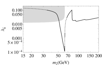
Figure 1: Along the curves the relic abundance constraint is satisfied. The dashed region are excluded by Fermi-LAT (left) and Fermi-LAT + MAGIC (right). The gray shaded region is excluded by the LHC experiment (see the next section).

4 Indirect Detection and Collider Bounds

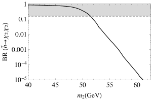
Figure 2: Left panel: Invisible branching ratio for the Higgs boson decay into a pair of pGDMs (solid line) along which $\Omega_{DM}h^{2}=0.120$ is reproduced, together with the LHC constraint (gray shaded). Right panel: The pGDM pair annihilation cross section into a pair of bottom quarks (solid curve) along which $\Omega_{DM}h^{2}=0.120$ is reproduced, together with the upper bounds from Fermi-LAT (dashed line) and the combined Fermi-LAT and MAGIC (dotted line).

Since the pGDM evades the direct DM detection constraints, we consider the constraints from the LHC and indirect DM detection experiments. Let us first consider the LHC bound. If kinematically allowed $(m_{2}<m_{{\tilde{h}}}/2)$, the SM Higgs boson can decay to a pair of pGDMs with a branching ratio,

$$BR({\tilde{h}}\to\chi_{2}\chi_{2})=\frac{\Gamma({\tilde{h}}\to\chi_{2}\chi_{2})}{\Gamma_{\tilde{h}}}.$$ (4.1)

The CMS result on the invisible Higgs boson decay at the LHC provides us with an upper bound, $BR({\tilde{h}}\to\chi_{2}\chi_{2})\leq 0.16$ [5]. In Fig. 2 (left panel), we show $BR({\tilde{h}}\to\chi_{2}\chi_{2})$ as a function of the DM mass (solid line) along which $\Omega_{DM}h^{2}=0.120$ is satisfied, together with the CMS constraint (gray shaded).

Next, let us consider the indirect DM detection constraints. A pair of pGDMs can annihilate into SM particles whose subsequent decays produce gamma-rays. Such gamma-rays originating from DM pair annihilations have been searched for by Fermi-LAT and MAGIC experiments. For a pGDM mass $\lesssim 80$ GeV, a pair of pGDMs dominantly annihilates into a pair of bottom quarks. We interpret the upper bounds on the annihilation cross section from the Fermi-LAT and MAGIC experiments into our model parameter space. Using the earlier result for $\lambda_{HB}$ as a function of $m_{2}$, we calculate the pGDM pair annihilation cross section into a pair of bottom quarks. In Fig. 2 (right panel), we show our result (solid curve), along with the upper bound from the Fermi-LAT result (dashed line) and the combined result by Fermi-LAT and MAGIC (dotted line). The regions of $m_{2}\lesssim 40$ GeV and $m_{2}\simeq m_{\tilde{h}}/2$ are excluded.

5 Conclusions

The Higgs-portal scalar DM scenario is one of the simplest extensions of the SM with a DM candidate. However, this scenario is very severely constrained by the null results from the direct DM detection experiments with nearly all of the parameter region excluded. The recently proposed pGDM scenario realizes the Higgs-portal scalar DM particle as a pseudo-Goldstone boson. Due to its Goldstone boson nature, the scattering cross section of the pGDM with a nucleon vanishes in the zero-momentum transfer limit, and so it evades the direct DM detection constraints.

We have proposed a pGDM scenario in the context of a gauged $B-L$ extension of the SM. Our model is a minimal extension of the well-known $B-L$ model with an additional $B-L$ Higgs field $\Phi_{B}$, and following the $B-L$ symmetry breaking, the Higgs sector of the model effectively realizes the pGDM scenario. Since the $B-L$ symmetry forbids the unwanted terms in the original pGDM model which explicitly break the global U(1) symmetry and thereby spoil the Goldstone boson nature of the DM particle, our model can be considered as a (gauged) ultraviolet completion of the pGDM scenario. Unlike the original model, the pGDM particle decays through the $B-L$ gauge interaction, and the $B-L$ symmetry breaking scale is estimated to be quite high ($\sim{\cal O}(10^{11})$ GeV) in order to make the pGDM lifetime sufficiently long. Although the model is free from the direct DM detection constraints, the DM model parameter space can be constrained by the LHC and gamma ray observations by Fermi-LAT and MAGIC.

Finally, in addition to the pGDM physics, our model retains the salient features of the minimal $B-L$ model such that the seesaw mechanism is automatically incorporated and the baryon asymmetry of the universe can be reproduced through leptgenesis. In short, our model overcomes three major problems of the SM, namely the origin of tiny neutrino masses, the nature of the DM particle, and the origin of matter-antimatter asymmetry.

Note added: While finalizing this manuscript we learned that the model we have proposed in this paper has very recently also been discussed by the authors of Ref. [17].

References

• [1] N. Aghanim et al. [Planck Collaboration], “Planck 2018 results. VI. Cosmological parameters,” arXiv:1807.06209 [astro-ph.CO].
• [2] J. McDonald, “Gauge singlet scalars as cold dark matter,” Phys. Rev. D 50, 3637 (1994) [hep-ph/0702143 [HEP-PH]]; C. P. Burgess, M. Pospelov and T. ter Veldhuis, “The Minimal model of nonbaryonic dark matter: A Singlet scalar,” Nucl. Phys. B 619, 709 (2001) [hep-ph/0011335].
• [3] E. Aprile et al. [XENON Collaboration], “Dark Matter Search Results from a One Ton-Year Exposure of XENON1T,” Phys. Rev. Lett.  121, no. 11, 111302 (2018) [arXiv:1805.12562 [astro-ph.CO]].
• [4] P. Agnes et al. [DarkSide Collaboration], “Low-Mass Dark Matter Search with the DarkSide-50 Experiment,” Phys. Rev. Lett.  121, no. 8, 081307 (2018) [arXiv:1802.06994 [astro-ph.HE]].
• [5] A. M. Sirunyan et al. [CMS Collaboration], “Search for invisible decays of a Higgs boson produced through vector boson fusion in proton-proton collisions at $\sqrt{s}=$ 13 TeV,” Phys. Lett. B 793, 520 (2019) [arXiv:1809.05937 [hep-ex]].
• [6] G. Arcadi, A. Djouadi and M. Raidal, “Dark Matter through the Higgs portal,” arXiv:1903.03616 [hep-ph].
• [7] C. Gross, O. Lebedev and T. Toma, “Cancellation Mechanism for Dark-Matter-Nucleon Interaction,” Phys. Rev. Lett.  119, no. 19, 191801 (2017) [arXiv:1708.02253 [hep-ph]].
• [8] J. C. Pati and A. Salam, “Lepton Number as the Fourth Color,” Phys. Rev. D 10, 275 (1974) Erratum: [Phys. Rev. D 11, 703 (1975)]; A. Davidson, “$B-L$ as the fourth color within an $\mathrm{SU}(2)_{L}\times\mathrm{U}(1)_{R}\times\mathrm{U}(1)$ model,” Phys. Rev. D 20, 776 (1979); R. N. Mohapatra and R. E. Marshak, “Local B-L Symmetry of Electroweak Interactions, Majorana Neutrinos and Neutron Oscillations,” Phys. Rev. Lett.  44, 1316 (1980) Erratum: [Phys. Rev. Lett.  44, 1643 (1980)]; “Quark - Lepton Symmetry and B-L as the U(1) Generator of the Electroweak Symmetry Group,” Phys. Lett.  91B, 222 (1980); C. Wetterich, “Neutrino Masses and the Scale of B-L Violation,” Nucl. Phys. B 187, 343 (1981); A. Masiero, J. F. Nieves and T. Yanagida, “$B^{-}$l Violating Proton Decay and Late Cosmological Baryon Production,” Phys. Lett.  116B, 11 (1982); R. N. Mohapatra and G. Senjanovic, “Spontaneous Breaking of Global $B-L$ Symmetry and Matter-Antimatter Oscillations in Grand Unified Theories,” Phys. Rev. D 27, 254 (1983); W. Buchmuller, C. Greub and P. Minkowski, “Neutrino masses, neutral vector bosons and the scale of B-L breaking,” Phys. Lett. B 267, 395 (1991).
• [9] M. Fukugita and T. Yanagida, “Baryogenesis Without Grand Unification,” Phys. Lett. B 174, 45 (1986).
• [10] M. Ackermann et al. [Fermi-LAT], “Searching for Dark Matter Annihilation from Milky Way Dwarf Spheroidal Galaxies with Six Years of Fermi Large Area Telescope Data,” Phys. Rev. Lett. 115, no.23, 231301 (2015) [arXiv:1503.02641 [astro-ph.HE]].
• [11] J. Aleksić, S. Ansoldi, L. A. Antonelli, P. Antoranz, A. Babic, P. Bangale, U. Barres de Almeida, J. A. Barrio, J. Becerra González and W. Bednarek, et al. “Optimized dark matter searches in deep observations of Segue 1 with MAGIC,” JCAP 02, 008 (2014) [arXiv:1312.1535 [hep-ph]].
• [12] M. L. Ahnen et al. [MAGIC and Fermi-LAT], “Limits to Dark Matter Annihilation Cross-Section from a Combined Analysis of MAGIC and Fermi-LAT Observations of Dwarf Satellite Galaxies,” JCAP 02, 039 (2016) [arXiv:1601.06590 [astro-ph.HE]]; L. Roszkowski, E. M. Sessolo and S. Trojanowski, “WIMP dark matter candidates and searches—current status and future prospects,” Rept. Prog. Phys. 81, no.6, 066201 (2018) [arXiv:1707.06277 [hep-ph]].
• [13] N. Okada and O. Seto, “Probing the seesaw scale with gravitational waves,” Phys. Rev. D 98, no. 6, 063532 (2018) [arXiv:1807.00336 [hep-ph]].
• [14] N. Okada and O. Seto, “Inelastic extra $U(1)$ charged scalar dark matter,” arXiv:1908.09277 [hep-ph].
• [15] R. Essig, E. Kuflik, S. D. McDermott, T. Volansky and K. M. Zurek, “Constraining Light Dark Matter with Diffuse X-Ray and Gamma-Ray Observations,” JHEP 1311, 193 (2013) [arXiv:1309.4091 [hep-ph]].
• [16] W. L. Guo and Y. L. Wu, “The Real singlet scalar dark matter model,” JHEP 1010, 083 (2010) [arXiv:1006.2518 [hep-ph]].
• [17] Y. Abe, T. Toma and K. Tsumura, “Pseudo-Nambu-Goldstone dark matter from gauged $U(1)_{B-L}$ symmetry,” arXiv:2001.03954 [hep-ph].