On the decoding of Barnes-Wall lattices

Abstract

We present new efficient recursive decoders for the Barnes-Wall lattices based on their squaring construction. The analysis of the new decoders reveals a quasi-quadratic complexity in the lattice dimension and a quasi-linear complexity in the list-size. The error rate is shown to be close to the universal lower bound in dimensions 64 and 128.

I Introduction

Barnes-Wall ($BW$) lattices were one of the first series discovered with an infinitely increasing fundamental coding gain [2]. This series includes dense lattices in lower dimensions such as $D_{4}$, $E_{8}$, $\Lambda_{16}$ [5], and is deeply related to Reed-Muller codes [9][17]: $BW$ lattices admit a Construction D based on these codes. Multilevel constructions attracted the recent attention of researchers, mainly Construction C^∗ [3], where lattice and non-lattice constellations are made out of binary codes. One of the important challenges is to develop lattices with a reasonable-complexity decoding where a fraction of the fundamental coding gain is sacrificed in order to achieve a lower kissing number. $BW$ lattices are attractive in this sense. For instance the lattice $BW_{128}$, with an equal fundamental coding gain as $Nebe_{72}$ [20], sacrifices 1.5 dB of its fundamental coding gain with respect to $MW_{128}$ [8] while the kissing number is reduced by a factor of 200.

Several algorithms have been proposed to decode $BW$ lattices. Forney introduced an efficient maximum-likelihood decoding (MLD) algorithm in [9] for the low dimension instances of these lattices based on their trellis representation. Nevertheless, the complexity of this algorithm is exponential in the dimension and intractable for $n>32$: e.g. decoding in $BW_{64}$ involves $2\cdot 2^{24}+2\cdot 2^{16}$ decoders of $BW_{16}$ and decoding in $BW_{128}$ involves $2\cdot 2^{48}+2\cdot 2^{32}$ decoders of $BW_{32}$ (using the two-level squaring construction to build the trellis, see [9, Section IV.B]). Later, [19] proposed the first bounded-distance decoders (BDD) running in polynomial time: a parallelisable decoder of complexity $O(n^{2})$ and another sequential decoder of complexity $O(n\log^{2}(n))$. The parallel decoder was generalized in [14] to work beyond the packing radius, still in polynomial time. It is discussed later in the paper. The sequential decoder uses the $BW$ multilevel construction to perform multistage decoding: each of the $\approx\log(n)$ levels is decoded with a Reed-Muller decoder of complexity $n\log(n)$. This decoder was also further studied, in [15], to design practical schemes for communication over the AWGN channel. The performance of this sequential decoder is far from MLD. A simple information-theoretic argument explains why multistage decoding of $BW$ lattices cannot be efficient: the rates of some component Reed-Muller codes exceed the channel capacities of the corresponding levels [13][28]. As a result, no $BW$ decoders, being both practical and quasi-optimal on the Gaussian channel, have been designed and executed for dimensions greater than $32$.

We present new decoders for $BW$ lattices based on their $(u,u+v)$ construction [17]. We particularly consider this construction as a squaring construction [9] to establish a new recursive BDD (Algorithm 2, Section III-A), new recursive list decoders (Algorithms 3 and 5, Sections IV-B and IV-C), and their complexity analysis as stated by Theorems 2-4. As an example, Algorithm 5 decodes $BW_{64}$ and $BW_{128}$ with a performance close to the universal lower bound on the coding gain of any lattice and with a reasonable complexity almost quadratic in the lattice dimension.

II preliminaries

Lattice. A lattice $\Lambda$ is a discrete additive subgroup of $\mathbb{R}^{n}$. For a rank-$n$ lattice in $\mathbb{R}^{n}$, the rows of a $n\times n$ generator matrix $G$ constitute a basis of $\Lambda$ and any lattice point $x$ is obtained via $x=zG$, where $z\in\mathbb{Z}^{n}$. The squared minimum Euclidean distance of $\Lambda$ is $d(\Lambda)=(2\rho(\Lambda))^{2}$, where $\rho(\Lambda)$ is the packing radius. The number of lattice points located at a distance $\sqrt{d(\Lambda)}$ from the origin is the kissing number $\tau(\Lambda)$. The fundamental volume of $\Lambda$, i.e. the volume of its Voronoi cell and its fundamental parallelotope, is denoted by $\text{vol}(\Lambda)$. The fundamental coding gain $\gamma(\Lambda)$ is given by the ratio $\gamma(\Lambda)=d(\Lambda)/\text{vol}(\Lambda)^{\frac{2}{n}}$. The squared Euclidean distance between a point $y\in\mathbb{R}^{n}$ and a lattice point $x\in\Lambda$ is denoted $d(x,y)$. Accordingly, the squared distance between $y\in\mathbb{R}^{n}$ and the closest lattice point of $\Lambda$ is $d(y,\Lambda)$.
For lattices, the transmission rate used with finite constellations is meaningless. Poltyrev introduced the generalized capacity [22], the analog of Shannon capacity for lattices. The Poltyrev limit corresponds to a noise variance of $\sigma^{2}_{max}=\det(\Lambda)^{\frac{2}{n}}/(2\pi e)$ and the point error rate is evaluated with respect to the distance to Poltyrev limit, i.e. $\sigma^{2}_{max}/\sigma^{2}$.

BDD, list-decoding, and MLD. Given a lattice $\Lambda$, a radius $r>0$, and any point $y\in\mathbb{R}^{n}$, the task of a decoder is to determine all points $x\in\Lambda$ satisfying $d(x,y)\leq r^{2}(\Lambda).$ If $r<\rho(\Lambda)$, there is either no point or a unique point found and the decoder is known as BDD. Additionally, if $d(x,y)<\rho^{2}(\Lambda)$, we say that $y$ is within the guaranteed error-correction radius of the lattice. If $r\geq\rho(\Lambda)$, there may be more than one point in the sphere. In this case, the process is called list-decoding rather than BDD. When list-decoding is used, lattice points within the sphere are enumerated and the decoded lattice point is the closest to $y$ among them. MLD simply refers to finding the closest lattice point in $\Lambda$ to any point $y\in\mathbb{R}^{n}$. If list-decoding is used, MLD is equivalent to choosing a decoding radius equal to $R(\Lambda)$.

Coset decomposition of a lattice. Let $\Lambda$ and $\Lambda^{\prime}$ be two lattices such that $\Lambda^{\prime}\subseteq\Lambda$. If the order of the quotient group $\Lambda/\Lambda^{\prime}$ is $q$, then $\Lambda$ can be expressed as the union of $q$ cosets of $\Lambda^{\prime}$. We denote by $[\Lambda/\Lambda^{\prime}]$ a system of coset representatives for this partition. It follows that $\Lambda=\bigcup_{x_{i}\in[\Lambda/\Lambda^{\prime}]}\Lambda^{\prime}+x_{i}=\Lambda^{\prime}+[\Lambda/\Lambda^{\prime}].$
The $BW$ lattices. Let the scaling-rotation operator $R(2n)$ in dimension $2n$ be defined by the application of the $2\times 2$ matrix

$$R(2)=\left[\begin{matrix}1&\ \ 1\\ 1&-1\end{matrix}\right]$$

on each pair of components. I.e. the scaling-rotation operator is $R(2n)=I_{n}\otimes R(2)$, where $I_{n}$ is the $n\times n$ identity matrix and $\otimes$ the Kronecker product. For $\Lambda\subset\mathbb{R}^{2n}$ with generator matrix $G$, the lattice generated by $G\cdot R(2n)$ is denoted $R\Lambda$.

Definition 1 (The squaring construction of $BW_{2n}$ [9]).

The $BW$ lattices in dimension $2n$ are obtained by the following recursion:

$$\begin{split}BW_{2n}&=\{(\underset{u_{1}\in BW_{n}}{\underbrace{v^{\prime}_{1}+m}},\underset{u_{2}\in BW_{n}}{\underbrace{v^{\prime}_{2}+m}}),v^{\prime}_{i}\in RBW_{n},m\in[BW_{n}/RBW_{n}]\},\end{split}$$

with initial condition $BW_{2}=\mathbb{Z}^{2}$.

Using this construction, it is easily seen that $d(BW_{2n})=d(RBW_{n})=2d(BW_{n})$ and the fundamental coding gain increases infinitely as $\gamma(BW_{n})=\sqrt{2}\cdot\gamma(BW_{n/2})=\sqrt{n/2}$ [9].
Note that the squaring construction can be expressed under the form of the Plotkin $(u,u+v)$ construction [21]:

$$BW_{2n} =\{(v^{\prime}_{1}+m,v^{\prime}_{2}+m),\ v^{\prime}_{i}\in RBW_{n},m\in[BW_{n}/RBW_{n}]\},$$

$$=\{(v^{\prime}_{1}+m,\underset{v^{\prime}_{2}}{\underbrace{v^{\prime}_{1}+v_{2}}}+m)\}=\{(u_{1},u_{1}+v_{2})\}.$$

III Bounded-distance $BW$ decoding

III-A The new BDD

Given a point $y=(y_{1},y_{2})\in\mathbb{R}^{2n}$ to be decoded, a well-known algorithm [26][7] for a code obtained via the $(u,u+v)$ construction is to first decode $y_{1}$ as $u_{1}$, and then decode $y_{2}-u_{1}$ as $v_{2}$ . Our lattice decoder, Algorithm 1, is double-sided since we also decode $y_{2}$ as $u_{2}$ and then $y_{1}-u_{2}$ as $v_{2}$: the decoder is based on the squaring construction. The main idea exploited by the algorithm is that if there is too much noise on one side, e.g. $y_{1}$, then there is less noise on the other side, e.g. $y_{2}$, and vice versa.

Algorithm 1 Double-sided $(u,u+v)$ decoder of $BW_{2n}$

Input: $y=(y_{1},y_{2})\in\mathbb{R}^{2n}$.

1:  Decode (MLD) $y_{1},y_{2}$ in $BW_{n}$ as $u_{1},u_{2}$.

2:  Decode (MLD) $y_{2}-u_{1}$ in $RBW_{n}$ as $v_{2}$. Store $\hat{x}\leftarrow(u_{1},u_{1}+v_{2})$.

3:  Dec. (MLD) $y_{1}-u_{2}$ in $RBW_{n}$ as $v_{1}$. Store $\hat{x}^{\prime}\leftarrow(u_{2}+v_{1},u_{2})$.

4:  Return $x_{dec}=\underset{x\in\{\hat{x},\hat{x}^{\prime}\}}{\text{argmin \ \ }}||y-x||$

Theorem 1.

Let $y$ be a point in $\mathbb{R}^{2n}$ such that $d(y,BW_{2n})$ is less than $\rho^{2}(BW_{2n})$. Then, Algorithm 1 outputs the closest lattice point $x\in BW_{2n}$ to $y$.

Proof.

If $(x_{1},x_{2})\in BW_{2n}$, then $x_{1},x_{2}\in BW_{n}$. Also, we have $||(y_{1},y_{2})||^{2}=||y_{1}||^{2}+||y_{2}||^{2}$. So if $d(y,BW_{2n})<~{}\rho^{2}(BW_{2n})$, then at least one among the two $y_{i}$ is at a distance smaller than $\frac{\rho^{2}(BW_{2n})}{2}=\rho^{2}(BW_{n})$ from $BW_{n}$. Therefore, at least one of the two $u_{i}$ is correct.
Assume (without loss of generality) that $u_{1}$ is correct. We have $d(y_{2}-u_{1},RBW_{n})<\rho^{2}(BW_{2n})=\rho^{2}(RBW_{n})$. Therefore, $y_{2}-u_{1}$ is also correctly decoded.
As a result, among the two lattice points stored, at least one is the closest lattice point to $y$. ∎

Note that the $BW_{n}$ decoder in the previous proof got exploited up to $\rho^{2}(BW_{n})$ only. Consequently, Algorithm 1 should exceed the performance predicted by Theorem 1 given that step 1 is MLD.
Algorithm 1 can be generalized into the recursive Algorithm 2, where Steps 4, 5, and 6 of the latter algorithm replace Steps 1, 2, and 3 of Algorithm 1, respectively. This algorithm is similar to the parallel decoder of [19]. The main difference is that [19] uses the automorphism group of $BW_{2n}$ to get four candidates at each recursion whereas we use the squaring construction to generate only two candidates. Nevertheless, both our algorithm and [19] use four recursive calls at each recursive section and have the same asymptotic complexity.

Algorithm 2 Recursive BDD of $BW_{2n}$ (where $2n=2^{t}$)

Function $RecBW(y,t)$
Input: $y=(y_{1},y_{2})\in\mathbb{R}^{2^{t}}$, $1\leq t$.

1:  if t = 1 then

2:     $x_{dec}\leftarrow(\lfloor y_{1}\rceil,\lfloor y_{2}\rceil)$     // Decoding in $\mathbb{Z}^{2}$

3:  else

4:     $u_{1}\leftarrow RecBW(y_{1},t-1)$, $u_{2}\leftarrow RecBW(y_{2},t-1)$ // $y_{2}-u_{1}$ (and $y_{1}-u_{2}$) should be decoded in $RBW_{n}$: // this is equivalent to decoding $(y_{2}-u_{1})\cdot R(2^{t-1})^{-1}$ in $BW_{n}$ // and then rotate the output lattice point by $R(2^{t-1})$.

5:     $v_{2}\leftarrow RecBW((y_{2}-u_{1})\cdot R(2^{t-1})^{T}/2,t-1)\cdot R(2^{t-1})$. Store $\hat{x}\leftarrow(u_{1},u_{1}+v_{2})$.

6:     $v_{1}\leftarrow RecBW((y_{1}-u_{2})\cdot R(2^{t-1})^{T}/2,t-1)\cdot R(2^{t-1})$. Store $\hat{x}^{\prime}\leftarrow(u_{2}+v_{1},u_{2})$.

7:     $x_{dec}=\underset{x\in\{\hat{x},\hat{x}^{\prime}\}}{\text{argmin \ \ }}||y-x||$

8:  end if

9:  Return $x_{dec}$

Theorem 2.

Let $n$ be the dimension the lattice $BW_{n}$ to be decoded. The complexity of Algorithm 2 is $O(n^{2})$.

Proof.

Let $\mathfrak{C}(n)$ be the complexity of the algorithm for $n=2^{t}$. We have $\mathfrak{C}(n)=4\mathfrak{C}(n/2)+O(n)=O(n^{2}).$∎

III-B Performance on the Gaussian channel

In the appendix (see Section VII-A), we show via an analysis of the effective error coefficient of Algorithm 2 that the loss in performance of this algorithm compared to MLD (in dB) is expected to grow linearly with $n$.
Our simulations show that there is a loss of $\approx$0.25 dB for $n=16$, $\approx$0.5 dB for $n=32$, $\approx$1.25 dB for $n=64$ (compare $\aleph=1$ and $\aleph=20$ on Figure 1) and $\approx$2.25 dB for $n=128$. As a result, this BDD is not suited for effective decoding of $BW$ lattices on the Gaussian channel. However, it is essential for building efficient decoders as shown in the next section.

IV List-decoding of $BW$ lattices beyond the packing radius

Let $L(\Lambda,r^{2})$ be the maximum number of lattice points of $\Lambda$ within a sphere of radius $r$ around any $y\in\mathbb{R}^{n}$. If $\Lambda=BW_{n}$ we write $L(n,r^{2})$. The following lemma is proved in [14].

Lemma 1.

The list size of the $BW_{n}$ lattices is bounded as [14]:

• $L(n,r^{2})\leq\frac{1}{2\epsilon}$ if $r^{2}\leq d(BW_{n})(1/2-\epsilon)$, $0<\epsilon\leq 1/4$.

• $L(n,r^{2})=2n$ if $r^{2}=d(BW_{n})/2$.

• $L(n,r^{2})\leq 2n^{16\log_{2}(1/\epsilon)}$ if $r^{2}\leq d(BW_{n})(1-\epsilon)$, $0~{}<~{}\epsilon~{}\leq~{}1/2$.

[14] also shows that the parallel BDD of [19], which uses the automorphism group of $BW_{n}$, can be slightly modified to output a list of all lattice points lying at a squared distance $r^{2}=d(BW_{n})(1-\epsilon),\forall\epsilon>0$, from any $y\in\mathbb{R}^{n}$ in time $O(n^{2})\cdot L(n,r^{2})^{2}$. With Lemma 1, this becomes $n^{O(\log(1/\epsilon))}$. This result is of theoretical interest: it shows that there exists a polynomial time algorithm in the dimension for any radius bounded away from the minimum distance. However, the quadratic dependence in the list-size is a drawback: finding an algorithm with quasi-linear dependence in the list-size is stated as an open problem in [14].

In the following, we show that if we use the squaring construction rather than the automorphism group of $BW_{n}$ for list-decoding, it is possible to get a quasi-linear complexity in the list size. This enables to get a practical list-decoding algorithm up to $n=128$.

IV-1 Some notations

Notice that $L(n,r^{2})=L(RBW_{n},2r^{2})$, e.g. both are equal to $2n$ if $r^{2}=d(BW_{n})/2$. It is therefore convenient to consider the relative squared distance as in [14]: $\delta(x,y)=\frac{d(x,y)}{d(\Lambda)}$, $x\in\Lambda$ . Then, if we define $l(\Lambda,r^{2}/d(\Lambda))=L(\Lambda,r^{2})$ this yields for instance $l(n,1/2)=l(BW_{n},1/2)=l(RBW_{n},1/2)=2n$. The relative squared radius is defined as the quantity $r^{2}/d(\Lambda)$. For the rest of this section, $\delta$ is the relative squared radius considered for decoding. Let $y=(y_{1},y_{2})\in\mathbb{R}^{2n}$ and $x=(u_{1},u_{1}+v_{2})=(u_{2}+v_{1},u_{2})\in BW_{2n}$ be any lattice point where $\delta(x,y)\leq\delta$. We recall that for BDD of $BW_{n}$ we have $\delta=1/4$.
The following lemma is trivial, but convenient to manipulate distances.

Lemma 2.

(Lemma 2.1 in [14])
Let $y=(y_{1},y_{2})\in\mathbb{R}^{2n}$ and $x=(u_{1},u_{1}+v_{2})\in~{}BW_{2n}$. Then,

$$\delta(x,y)=\delta(u_{1},y_{1})/2+\delta(v_{2},y_{2}-u_{1}).$$ (1)

IV-2 List-decoding with $r^{2}<9/16d(BW_{n})$

Assume that the squared norm of the noise is $r^{2}$ and $\delta=(r^{2}+\epsilon)/d(BW_{n})$. Consider $d(x,y)=d(u_{1},y_{1})+d(u_{2},y_{2})$. We split the possible situations into two main cases (similarly to Steps 2-3 of Algorithm 1): $d(u_{1},y_{1})\leq r^{2}/2$ and $d(u_{1},y_{1})>r^{2}/2$. For the first case, $y_{1}$ should be list-decoded in $BW_{n/2}$, and for each $u_{1}\in BW_{n/2}$ in the resulting list, $y_{2}-u_{1}$ should be list-decoded in $RBW_{n/2}$. Regarding the noise repartition, one can get the following two extreme configurations (but not simultaneously): $d(u_{1},y_{1})=r^{2}/2$, i.e. $\delta(u_{1},y_{1})=\delta$ and $d(v_{2},y_{2}-u_{1})=r^{2}$, i.e. $\delta(v_{2},y_{2}-u_{1})=\delta$. Consequently, without any advanced strategy, the relative squared decoding radius to list-decode in $BW_{n/2}$ and $RBW_{n/2}$ should be $\delta$. The maximum of the product of the two resulting list-sizes, which is a key element in the complexity analysis below, is $l(n/2,\delta)^{2}$. In order to reduce this number, we split this first case (i.e. $d(u_{1},y_{1})\leq r^{2}/2$) into two sub-cases. Let $0\leq a^{\prime}\leq r^{2}/2$.

• $0\leq d(u_{1},y_{1})<a^{\prime}$ and $r^{2}/2<d(v_{2},y_{2}-u_{1})\leq r^{2}$: then, $y_{1}$ should be list-decoded in $BW_{n/2}$ with a relative squared radius $a_{1}=a^{\prime}/d(BW_{n/2})$ and $y_{2}-u_{1}$ list decoded in $RBW_{n/2}$ with a relative squared radius $\delta$.

• $a^{\prime}\leq d(u_{1},y_{1})\leq r^{2}/2$ and $r^{2}/2<d(v_{2},y_{2}-u_{1})\leq r^{2}-a^{\prime}$: then, $y_{1}$ should be list-decoded in $BW_{n/2}$ with a relative squared radius $\delta$ and $y_{2}-u_{1}$ list-decoded in $RBW_{n/2}$ with a relative squared radius $a_{2}=(r^{2}-a^{\prime})/d(RBW_{n/2})$.

The size of the two resulting lists are bounded by $l(n/2,a_{1})\cdot l(RBW_{n/2},\delta)$ and $l(n/2,\delta)\cdot l(RBW_{n/2},a_{2})$. Consequently, if we choose $a_{1}=a_{2}=a$, i.e. $a=2/3\delta$, the two bounds are equal. The maximum number of candidates to consider becomes $2l(n/2,\delta)\cdot l(n/2,a)$ which is likely to be much smaller than $l(n/2,\delta)^{2}$, the bound obtained without the splitting strategy. The second case (i.e. $d(u_{1},y_{1})>r^{2}/2$) is identical by symmetry.

This analysis yields Algorithm 3 listed below. The “removing step” (10 in bold) is added to ensure that a list with no more than $l(n,\delta)$ elements is returned by each recursive call. The maximum number of points to process by this removing step is $4l(n/2,\delta)l(n/2,a)$. Regarding Step 11, using the classical Merge Sort algorithm, it can be done in
$O(n\cdot l(n,\delta)\log(l(n,\delta)))$ operations (see App. VII-B).

The following theorem shows that we get an algorithm of quasi-linear complexity in the list size $l(n,\delta)$.

Theorem 3.

Given any point $y\in\mathbb{R}^{n}$ and $1/4\leq\delta<9/16$, Algorithm 3 outputs the list of all lattice points in $BW_{n}$ lying within a sphere of relative squared radius $\delta$ around $y$ in time:

• $O(n^{2}\log n)l(n,\delta)+O(n\log n)l(n,\delta)\log l(n,\delta)$
  if $1/4\leq\delta<3/8$

• $O(n^{1+\log_{2}(1+l(n,2/3\delta))}\log n)l(n,\delta)l(n,2/3\delta)+$
  $O(n^{\log_{2}(1+l(n,2/3\delta))})l(n,\delta)\log l(n,\delta)$ if $3/8\leq\delta<9/16$.

Proof.

Let $\mathfrak{C}(n,\delta)$ be the complexity of Algorithm 3. We have

$$\begin{split}\mathfrak{C}(n,\delta)&\leq\underset{\text{Numb. recursive calls with }\delta}{\underbrace{(2+2l(n/2,a))\mathfrak{C}(n/2,\delta)}}+\underset{\text{Numb. recursive calls with }a}{\underbrace{(2+2l(n/2,\delta))\mathfrak{C}(n/2,a)}}+\\ &\underset{\text{removing}}{\underbrace{4l(n/2,\delta)l(n/2,a)O(n)}}+\underset{\text{Merge Sort}}{\underbrace{O(n\cdot l(n,\delta)\log(l(n,\delta)))}}.\end{split}$$ (2)

If $\delta<3/8$, then $l(n,a)\leq 1$ and $\mathfrak{C}(n/2,a)\leq\mathfrak{C}(n/2,1/4)=O((n/2)^{2})$ (the complexity of Algorithm 2). (2) becomes

$$\begin{split}\mathfrak{C}(n,\delta)=O(n^{2}\log n)l(n,\delta)+O(n\log n)l(n,\delta)\log l(n,\delta).\end{split}$$ (3)

If $\delta<9/16$, then $\mathfrak{C}(n/2,a)<\mathfrak{C}(n/2,3/8)$. Using (3) for $\mathfrak{C}(n/2,3/8)$, (2) becomes

$$\begin{split}&\mathfrak{C}(n,\delta)=O(n^{1+\log_{2}(1+l(n,2/3\delta))}\log n)l(n,\delta)l(n,2/3\delta)+\\ &O(n^{\log_{2}(1+l(n,2/3\delta))})l(n,\delta)\log l(n,\delta)\end{split}$$

∎

Algorithm 3 First recursive list-decoding of $BW_{2n}$ ($2n=2^{t}$).

Function $ListRecBW(y,t,\delta)$
Input: $y=(y_{1},y_{2})\in\mathbb{R}^{2^{t}}$, $1\leq t$, $1/4\leq\delta<3/4$.

1:  $a\leftarrow 2/3\cdot\delta$

2:  $r\leftarrow\sqrt{2^{t-1}\cdot\delta}$

3:  if t = 1 then

4:     $\hat{x}\leftarrow Enum_{\mathbb{Z}_{2}}(y,r)$  // Enum. in $\mathbb{Z}^{2}$ with radius $r=\sqrt{\delta}$.

5:  else

6:     $\hat{x}_{1}\leftarrow SubRoutine(y_{1},y_{2},t,a,\delta,0)$

7:     $\hat{x}_{2}\leftarrow SubRoutine(y_{1},y_{2},t,\delta,a,0)$

8:     $\hat{x}_{3}\leftarrow SubRoutine(y_{2},y_{1},t,\delta,a,1)$

9:     $\hat{x}_{4}\leftarrow SubRoutine(y_{2},y_{1},t,a,\delta,1)$

10:     Remove all candidates at a distance $>r$ from $y$.

11:     Sort the remaining list of candidates in a lexicographic order and remove all duplicates.

12:  end if

13:  Return the list of all the candidates remaining.

Algorithm 4 Subroutine of Algorithms 3

Function $SubRoutine(y_{1},y_{2},t,\delta_{1},\delta_{2},reverse)$
Input: $y_{1},y_{2}\in\mathbb{R}^{2^{t-1}}$, $1\leq t$, $0<\delta_{1},\delta_{2}\leq 3/4$, $rev.~{}\in~{}\{0,1\}$.

1:  if $\delta_{1}\leq 1/4$ then

2:     $u_{1}\_List\leftarrow RecBW(y_{1},t-1)$

3:  else

4:     $u_{1}\_List\leftarrow ListRecBW(y_{1},t-1,\delta_{1})$

5:  end if

6:  for $u_{1}\in u_{1}\_List$ do

7:     if $\delta_{2}\leq 1/4$ then

8:        $v_{2}\_List(u_{1})\leftarrow RecBW((y_{2}~{}-~{}t_{1})~{}\cdot R(2^{t-1})^{T}/2,t~{}-~{}1)\cdot R(2^{t-1})$

9:     else

10:        $v_{2}\_List(u_{1})\leftarrow ListRecBW((y_{2}-t_{1})~{}\cdot R(2^{t-1})^{T}/2,t-1,\delta_{2})\cdot R(2^{t-1})$

11:     end if

12:  end for

13:  for $u_{1}\in u_{1}\_List$ do

14:     for $v_{2}\in v_{2}\_List(u_{1})$ do

15:        if $reverse=0$ then

16:           Compute and store $\hat{x}\leftarrow(u_{1},v_{2}+u_{1})$.

17:        else

18:           Compute and store $\hat{x}\leftarrow(v_{2}+u_{1},u_{1})$.

19:        end if

20:     end for

21:  end for

22:  Return the list of all candidates $\hat{x}$.

Unfortunately, the performance of Algorithm 3 on the Gaussian channel is disappointing. This is not surprising: notice that due to the “removing step” (10 in bold), some points that are correctly decoded by Algorithm 2 (the BDD) are not in the list outputted by Algorithm 3! Therefore, instead of removing all candidates at a distance greater than $r$, it is tempting to keep $\aleph$ candidates at each step.

IV-A An efficient list decoder on the Gaussian channel

We call Algorithm 5 a modified version of Algorithm 3 where the $\aleph(\delta)$ closest candidates are kept at each recursive step (instead of step 10, i.e. keeping only the points in the sphere of radius $r$) and steps 10 and 11 are flipped. The size of the list $\aleph(\delta)$, for a given $\delta$, is a parameter to be fine tuned: e.g. for $\delta=3/8$, one needs to choose only $\aleph(3/8)$ but for $\delta=1/2$, one needs to choose $\aleph(1/2)$ and $\aleph(2/3\cdot 1/2=1/3)$. The following theorem follows from Theorem 3.

Theorem 4.

Given any point $y\in\mathbb{R}^{n}$ and $1/4\leq\delta<9/16$, Algorithm 5 outputs the list of all lattice points in $BW_{n}$ lying within a sphere of relative squared radius $\delta$ around $y$ in time:

• $O(n^{2}\log n)\aleph(\delta)+O(n\log n)\aleph(\delta)\log\aleph(\delta)$
  $1/4\leq\delta<3/8$

• $O(n^{1+\log_{2}(1+\aleph(2/3\delta))}\log n)\aleph(\delta)\aleph(2/3\delta)+$
  $O(n^{\log_{2}(1+\aleph(2/3\delta))})\aleph(\delta)\log\aleph(\delta)$ if $3/8\leq\delta<9/16$.

Note that on the Gaussian channel, the probability that $y$ is exactly between two lattice points is 0. As a result, we can assume that $l(n,1/4)=1$ and thus include $\delta=3/8$ in the first case of Theorem 4.

As comparison, a similar modification of the algorithm of [14] would yield a complexity $O(n^{2})\cdot\aleph(\delta)^{2}$. In the next section on simulations, we show that for $n=32$ and $n=64$, one should choose $\delta=3/8$ and $\aleph(\delta)$ should be at least 10 and 20, respectively. Moreover, for $n=128$ quasi-optimal performance is achieved for $\delta=1/2$ with $\aleph(\delta)=1000$ and $\aleph(2/3\delta)=4$. With these parameters, our algorithm has a clear advantage thanks to the quasi-linear dependence in $\aleph(\delta)$.

V Numerical results

V-A Performance of Algorithm 5

Figure 1 shows the influence of the list size when decoding $BW_{64}$ using Algorithm 5 with $\delta=3/8$. On this figure we also plotted an estimate of the MLD performance of $BW_{64}$, obtained as $\tau(BW_{64})/2\cdot\text{erfc}(\gamma/(8\sigma^{2}_{max}/\sigma^{2}))$ [5, Chap. 3].

Figure 2 depicts the performance of Algorithm 5 for the $BW$ lattices up to $n=128$ and the universal bounds provided in [27] (see also [13] or [16], where it is called the sphere lower bound). These universal bounds are limits on the highest possible coding gain using $any$ lattice in $n$ dimensions. For each $BW_{n}$ we tried to reduce as much as possible the list size while keeping quasi-MLD performance. The choice of $\delta=3/8$ yields quasi-MLD performance up to $n=64$ with small list size and thus reasonable complexity. This shows that $BW_{64}$, with Algorithm 5, is a good candidate to design finite constellations in dimension 64. However, for $n=128$ one needs to set $\delta=1/2$ and choose $\aleph(\delta)=1000$. Nevertheless, $\aleph(2/3\cdot\delta)$ can be as small as 4, which is still tractable.

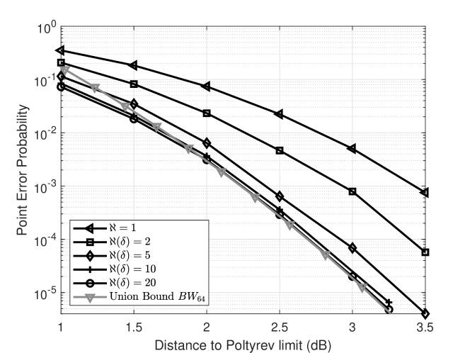
Figure 1: Influence of the list size when decoding $BW_{64}$ using Alg. 5, $\delta=3/8$.

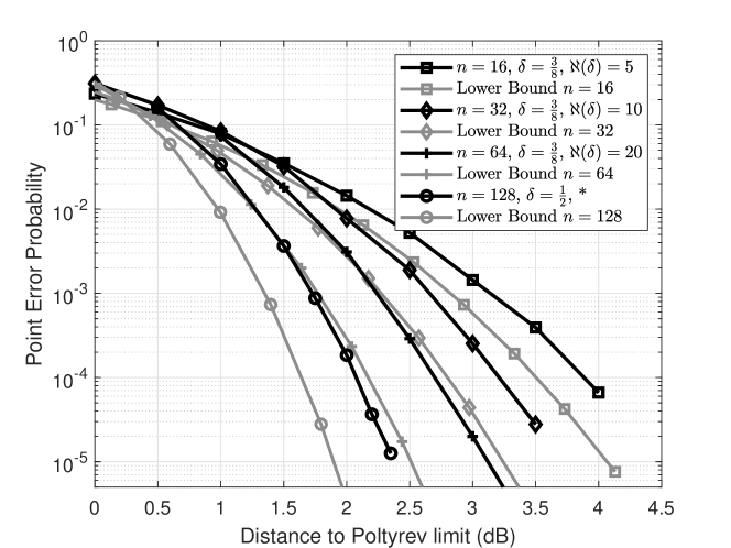
Figure 2: Algorithm 5 for the $BW$ lattices up to $n~{}=~{}128$ and the universal bounds of [27]. ^∗For $n=128$, $\aleph(\delta)=1000$ and $\aleph(2/3\delta)=4$.

We compare these performances with existing schemes at $P_{e}=10^{-5}$. For fair comparison between the dimensions, we let $P_{e}$ be either the normalized error probability, which is equal to the point error-rate divided by the dimension (as done in e.g. [27]), or the symbol error-rate.
First, several constructions have been proposed for block-lengths around $n=100$ in the literature. In [18] a two-level construction based on BCH codes with $n=128$ achieves this error-rate at 2.4 dB. The decoding involves an OSD of order 4 with 1505883 candidates. In [1] the multilevel (non-lattice packing) $\mathcal{S}_{127}$ ($n=127$) has similar performance but with much lower decoding complexity via generalized minimum distance decoding. In [23] a turbo lattice with $n=102$ and in [25] a LDLC with $n=100$ achieve the error-rate with iterative methods at respectively 2.75 dB and 3.7 dB (unsurprisingly, these two schemes are efficient for larger block-lengths). All these schemes are outperformed by $BW_{64}$, where $P_{e}=10^{-5}$ is reached at 2.3 dB. Moreover, $BW_{128}$ has $P_{e}=10^{-5}$ at $1.7$ dB, which is similar to many schemes with block-length $n=1000$ such as the LDLC (1.5 dB) [25], the turbo lattice (1.2 dB) [23], the polar lattice with $n=1024$ (1.45 dB) [28], and the LDA lattice (1.27 dB) [6]. This benchmark is summarized in Figure 3.

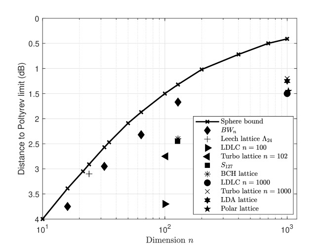
Figure 3: Perf. of different lattices for normalized error probability $P_{e}=10^{-5}$.

V-B Performance of $BW$ finite constellations

We uncover the performance of a Voronoi constellation [4][10] based on the partition $BW_{64}/2^{\eta}BW_{64}$ via Monte Carlo simulation, where $\eta$ is the desired rate in bits per channel use (bpcu): i.e. both the coding lattice and the shaping lattice are based on $BW_{64}$. It follows that the encoding complexity is the same as the decoding complexity: the complexity of Algorithm 5 with $\delta=3/8$ and $\aleph(\delta)=20$. Figure 4 exhibits the performance of our scheme for $\eta=4$ bpcu. In our simulation, the errors are counted on the uncoded symbols. The error-rate also includes potential errors due to incomplete encoding, which seem to be negligible compared to decoding errors. Again, we plotted the best possible performance of $any$ lattice-based constellation in dimension 64 (obtained from [27]). The scheme performs within 0.7 dB of the bound.

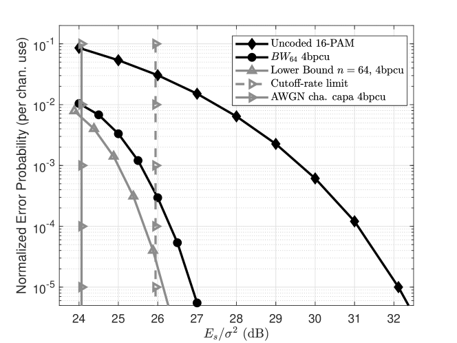
Figure 4: Performance of a Voronoi constellation based on the partition $BW_{64}/2^{4}BW_{64}$ where Algorithm 5, with $\delta=3/8$ and $\aleph(\delta)=20$, is used for encoding and decoding. The cutoff-rate limit is 1.7+0.179 dB right to Shannon limit (coding + shaping loss for $n=64$)[12].

VI Conclusions

Our recursive paradigm can be seen as a tree search algorithm and our decoders fall therefore in the class of sequential decoders. While the complexity of Algorithm 5 remains stable and low for $n\leq 64$, there is a significant increase for $n=128$ and it becomes intractable for $n=256$ due to larger lists. This is not surprising from the cut-off rate perspective [12]; For $n=64$ the MLD is still at a distance of $1$ dB from this limit (Figure 4), but it is very close to the limit for $n=128$ and potentially better at larger $n$. One should not expect to perform quasi-MLD of these lattices with any sequential decoder. This raises the following open problem: can we decode lattices beyond the cut-off rate in non-asymptotic dimensions, i.e. $n<300$, where classical capacity-approaching decoding techniques (e.g. BP) cannot be used?

VII Appendix

VII-A Analysis of the effective error coefficient

Let us define the decision region of a BDD algorithm $\mathbb{R}_{BDD}(\textbf{0})$ as the set of all points of the space that are decoded to 0 by the algorithm. The number of points at distance $\rho(\Lambda)$ from the origin that are not necessarily decoded to 0 are called boundary point of $\mathbb{R}_{BDD}(\textbf{0})$ The number of such points is called effective error coefficient of the algorithm. The performance of BDD algorithms are usually estimated via this effective error coefficient [11][24]. Indeed, BDD up to the packing radius achieves the best possible error exponent on the Gaussian channel, but the performance might be significantly degraded, compared to MLD, due to a high effective error coefficient.
In [19], the error coefficient of the parallel decoder is not computed and the performance of the algorithm is not assessed on the Gaussian channel. The following analysis of Algorithm 2 is also valid for the parallel decoder [19]. Let us express the point to be decoded as $y=x+\eta$, where $x\in BW_{n}$ and $\eta$ is a noise pattern. Scale $BW_{n}$ such that its packing radius is 1. It is easily seen that any $\eta$ of the form $(\pm\frac{1}{\sqrt{2^{t}}}^{2^{t}})=(\pm\frac{1}{\sqrt{2^{t}}},...,\pm\frac{1}{\sqrt{2^{t}}})$, $t=\log_{2}(n)$, is on the boundary of $\mathbb{R}_{BDD}(\textbf{0})$. The number of such noise patterns is $2^{2^{t}}=2^{n}$. According to Forney’s rule of thumb, every factor-of-two increase in the number of nearest neighbor results in a $0.2$ dB loss in effective coding gain [12]. Since the kissing number of $BW_{n}$ is $\prod_{i=1}^{t}(2^{i}+2)\approx 4.768...\cdot 2^{0.5log_{2}n(log_{2}n+1)}$ [5], to be compared to the above number of noise patterns $2^{n}$, we see that the loss in performance compared to MLD (in dB) is expected to grow as $\approx 0.2n$. However, this rule holds only if the effective error coefficient is not too large and the performance of Algorithm 2 is not as bad in practice. Nevertheless, this analysis hints that one should expect the performance of this BDD to degrade as $n$ increases.

VII-B The Merge Sort Algorithm

Let $l^{k,n}=(x_{1}^{n},x_{2}^{n}...,x_{k}^{n})$ be a list of $k$ elements $x$ of dimension $n$ (assume for the sake of simplicity that $k$ is a power of 2). This list can be split into two lists of equal size $l_{1}^{k/2,n}$ and $l_{2}^{k/2,n}$ and we write $l^{k,n}=(l_{1}^{k/2,n},l_{2}^{k/2,n})$.
Then, we define the function $Merge$ as a function that takes two sorted lists of $k$ elements $x$ of dimension $n$ as input (as well as $k$ and $n$) and returns a unique sorted list of the $2k$ elements. There exists several variants of this function, but the complexity is always $O(n\cdot k)$.

Algorithm 5 Merge Sort Algorithm

Function: $MS(l^{k,n},k,n)$
Input: $l^{k,n}=(l_{1}^{k/2,n},l_{2}^{k/2,n})$, $k\geq 1$, $n~{}\geq~{}1$.

1:  if $k=1$ then

2:     Return $l^{k,n}$.

3:  else

4:     Return $Merge(MS(l_{1}^{k/2,n},\frac{k}{2},n),M(l_{2}^{k/2,n},\frac{k}{2},n),k,n)$

5:  end if

Let $\mathfrak{C}(k,n)$ be the complexity of the $MS$ function (Algorithm 6). The complexity of this algorithm is $\mathfrak{C}(k,n)=2\mathfrak{C}(k/2,n)+O(k~{}\cdot~{}n)=O(k\log(k)\cdot n)$

References

- [1] D. Agrawal and A. Vardy, “Generalized minimum distance decoding in euclidean space: Performance analysis,” IEEE Trans. Inform. Theory, vol. 46, pp. 60–83, 2000.
- [2] E. S. Barnes and G. E. Wall, “Some extreme forms defined in terms of Abelian groups,” J. Australian Math. SOC., vol. 1, pp. 47-63, 1959.
- [3] M. F. Bollauf, R. Zamir, S. I. R. Costa, “Multilevel Constructions: Coding, Packing and Geometric Uniformity,” IEEE Trans. on Inform. Theory, Vol. 65, 2019.
- [4] J. Conway and N. Sloane, “A fast encoding method for lattice codes and quantizers,” IEEE Trans. Inform. Theory, vol. 19, pp. 820-824, 1983.
- [5] J. Conway and N. J. A. Sloane. Sphere packings, lattices and groups. Springer-Verlag, New York, 3rd edition, 1999.
- [6] N. di Pietro, J. J. Boutros, G. Zémor, L. Brunel, “Integer Low-Density Lattices based on Construction A”, 2012 IEEE Information Theory Workshop, 2012.
- [7] I. Dumer and K. Shabunov, “Soft-decision decoding of Reed-Muller codes: recursive lists,” IEEE Trans. Inform. Theory, vol. 52, pp. 1260-1266, 2006.
- [8] N. D. Elkies, “Mordell-Weil lattices in characteristic 2: III. A Mordell-Weil lattice of rank 128,” Experimental Math., vol. 3, pp. 467-473, 2001.
- [9] G. D. Forney, Jr., “Coset codes II: Binary lattices and related codes,” IEEE Trans. Inform. Theory, vol. 34, pp. 1152-1187, 1988.
- [10] G. D. Forney, Jr., “Multidimensional Constellations - part II: Voronoi Constellations,” IEEE J. Select. Areas Com., vol. 7, pp. 941-958, 1989.
- [11] G. D. Forney, Jr. and A. Vardy, “Generalized Minimum-Distance decoding of Euclidean-Space Codes and Lattices,” IEEE J. Select. Areas Com., vol. 42, pp. 1992-2026, 1996.
- [12] G. D. Forney and G. Ungerboeck, “Modulation and Coding for Linear Gaussian Channels,” IEEE Trans. Inform. Theory, vol. 44, pp. 2384-2415, 1998.
- [13] G. D. Forney, M. D. Trott, and S. Chung, “Sphere-Bound-Achieving Coset Codes and Multilevel Coset Codes,” IEEE Trans. Inform. Theory, vol. 46, pp. 820-850, 2000.
- [14] E. Grigorescu and C. Peikert, “List-Decoding Barnes-Wall Lattices,” Computational Complexity, vol. 26, pp 365-39, 2017.
- [15] J. Harshan, E. Viterbo, and J.-C. . Belfiore, “Practical Encoders and Decoders for Euclidean Codes from Barnes-Wall Lattices,” IEEE Trans. Communications, vol. 61, pp. 4417-4427, 2013.
- [16] A. Ingber, R. Zamir, and M. Feder, “Finite-Dimensional Infinite Constellations,” IEEE Trans. Inform. Theory, vol. 59, pp. 1630-1656, 2013.
- [17] F. J. MacWilliams and N. J. A. Sloane, The Theory of Error-Correcting Codes. Amsterdam, The Netherlands: North-Holland, 1977.
- [18] T. Matsumine, B. M. Kurkoski, and H. Ochiai, “Construction D Lattice Decoding and Its Application to BCH Code Lattices,” 2018 IEEE Global Communications Conference (GLOBECOM), 2018.
- [19] D. Micciancio and A. Nicolosi, “Efficient Bounded Distance Decoders for Barnes-Wall Lattices,” 2008 IEEE Int. Symp. Inform. Theory, 2008.
- [20] G. Nebe, “An even unimodular 72-dimensional lattice of minimum 8,” J. Reine Angew. Math., vol. 673, pp. 237-247, 2012.
- [21] M. Plotkin, “Binary codes with specified minimum distances,” IEEE Trans. Inform. Theory, vol. 6, pp. 445-450, 1960.
- [22] G. Poltyrev, “On coding without restrictions for the AWGN channel,” IEEE Trans. Inform. Theory, vol. 40, pp. 409-417, 1994.
- [23] A. Sakzad, M. Sadeghi, and D. Panario, “Turbo Lattices: Construction and Performance Analysis,” arXiv preprint arXiv:1108.1873, 2011. 48th Annual Allerton Conf. on Com., Control, and Computing , 2011.
- [24] A. J. Salomon and O. Amrani, “Encoding and Decoding Binary Product Lattices,” IEEE Trans. Inform. Theory, vol 52, pp 5485-5495, 2006.
- [25] N. Sommer, M. Feder, and O. Shalvi, “Low-density Lattice Codes,” IEEE Trans. Inform. Theory, vol. 54, pp. 1561-1585, 2008.
- [26] G. Schnabl and M. Bossert, “Soft-decision decoding of Reed-Muller codes as generalized multiple concatenated codes,” IEEE Trans. on Inform. Theory, vol. 41, pp. 304-308, 1995.
- [27] V. Tarokh, A. Vardy, and K. Zeger, “Universal bound on the performance of lattice codes,” IEEE Trans. Inform. Theory, vol. 45, pp. 670-681, 1999.
- [28] Y. Yan, C. Ling, X. Wu, “Polar lattices: Where Arıkan meets Forney,” 2013 IEEE Int. Symp. Inform. Theory, 20013.