The Early Stages of Heavy Ion Collisions

Abstract:

Heavy ion collisions pose interesting challenges to quantum chromodynamics, because they probe the parton structure of the incoming nuclei at very small longitudinal momentum fractions. Combined with the large size of nuclei, this may lead to the phenomenon of gluon saturation. The Color Glass Condensate is an effective QCD description that aims to cope with such a situation. In this talk, I show how one may study heavy ion collisions in this framework.

Lattice QCD has taught us that nuclear matter should undergo a transition at high temperature and/or density, by which the quarks and gluons confined into hadrons in ordinary conditions become deconfined. These conditions of temperature and density were most certainly reached in the early Universe, but the deconfined nuclear matter present at those times did not leave any visible imprint accessible to present day astronomy. These critical conditions can also be briefly accessed by colliding heavy nuclei at very high energy, as performed by the RHIC and the LHC.

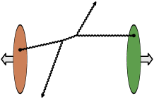
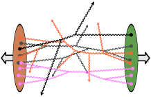
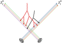
Figure 1: Left: collisions of dilute and dense projectiles. Right: color currents and radiated gauge field.

From the point of view of QCD, the main difficulty in studying these collisions is the fact that the nuclei are probed in a regime of large gluon density. In fact, not only the standard formalism of parton distributions becomes inadequate because it does not provide any information regarding multi-gluon distributions, but also gluons in this regime undergo non-linear interactions that limit the growth of their density, a phenomenon known as gluon saturation [1]. The color glass condensate [2] is an effective description of hadrons or nuclei in the dense regime, in which the projectiles are treated as color currents flowing along the light-cone. These currents are eikonally coupled to the gauge fields and become strong (of order $g^{-1}$) in the saturated regime, which leads to a peculiar power counting [3],

$$\raise-36.98857pt\hbox to113.81102pt{\includegraphics[width=113.81102pt]{PC3.pdf}}\;\sim\quad\underbrace{g^{n_{{}_{E}}-2}}_{\mbox{\scriptsize ext. lines}}\;\underbrace{(\hbar g^{2})^{n_{{}_{L}}}}_{\mbox{\scriptsize loops}}\;\underbrace{(g\,J)^{n_{j}}}_{\mbox{\scriptsize sources}},$$ (1)

where the number of insertions of the currents is irrelevant in the saturated regime (each connected vacuum graph is of order $g^{-2}$). In general, observables in the saturated regime are obtained as the sum of an infinite number of graphs, including both graphs connected to the measured gluons and disconnected vacuum graphs.

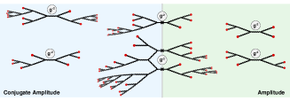
Figure 2: Diagrammatic expansion for a generic observable.

Inclusive observables are considerably simpler since the disconnected vacuum graphs drop out [3]. For instance, gluon production is determined at leading order uniquely by the sum of all the tree diagrams, i.e., by the classical solution of Yang-Mills equations (moreover, one can show that this solution must obey a null retarded boundary condition):

$$\overline{N}_{{}_{\rm LO}}=\quad\raise-1.99168pt\hbox to45.52458pt{\leavevmode\resizebox{45.52458pt}{}{\includegraphics{O_LO}}},\quad\raise-19.91692pt\hbox to284.52756pt{\leavevmode\resizebox{284.52756pt}{}{\includegraphics{classfield}}}$$ (2)

An important question in the context of heavy ion collisions is that of the thermalization of the produced gluonic matter. Immediately after the collision, this matter is far off-shell, made of color fields whose electric and magnetic components are parallel to the collision axis [4]. Consequently, the initial longitudinal pressure is exactly the opposite of the energy density. By solving numerically the classical Yang-Mills equations, one observes that the longitudinal pressure increases and reaches positive values at a time $Q_{s}\tau\sim 1$, but never becomes comparable to the transverse pressure (in fact, at leading order, this system appears to be a free-streaming collection of gluons) [5, 6].

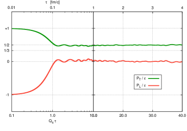
Figure 3: Time evolution of the transverse and longitudinal pressures at leading order.

The next order is made of all the one-loop graphs, in the presence of the external currents representing the projectiles, as illustrated here:

$${\cal O}_{{}_{\rm LO}}[J]=\raise-42.67912pt\hbox to136.57323pt{\leavevmode\resizebox{136.57323pt}{}{\includegraphics{tree_LO_st}}},\quad{\cal O}_{{}_{\rm NLO}}[J]=\raise-42.67912pt\hbox to136.57323pt{\leavevmode\resizebox{136.57323pt}{}{\includegraphics{tree_NLO}}}$$ (3)

In the case of inclusive observables, such a one-loop correction can be related to the leading order contribution [7]. The causal nature of the classical field encountered at leading order plays a crucial role in these manipulations. Loosely speaking, this amounts to first extending the original observable so that it depends on a field with a non-null initial condition, and then to note that the one-loop correction to this generalized quantity can be obtained by the action of an operator which is quadratic in derivatives with respect to the initial value of the field. Diagrammatically, this relationship reads

$${\cal O}_{{}_{\rm NLO}}[J,{\cal A}_{\rm in}]=\raise-42.67912pt\hbox to128.0374pt{\leavevmode\resizebox{128.0374pt}{}{\includegraphics{tree_NLO1}}},\quad{\cal O}_{{}_{\rm NLO}}[J,{\cal A}_{\rm in}]=\raise-42.67912pt\hbox to128.0374pt{\leavevmode\resizebox{128.0374pt}{}{\includegraphics{tree_NLO3}}},$$ (4)

while a more precise version is

$${\cal O}_{{}_{\rm{NLO}}}[J,{\cal A}_{\rm in}]=\Bigg{[}\frac{{\hbar}}{2}\int d^{3}\mathbf{x}d^{3}\mathbf{y}\;{{\Gamma}(\mathbf{x},\mathbf{y})}\;\frac{\delta}{\delta{\cal A}_{\rm in}(\mathbf{x})}\frac{\delta}{\delta{\cal A}_{\rm in}(\mathbf{y})}\Bigg{]}\;\vphantom{\frac{\delta}{\delta{\cal A}_{\rm in}(\mathbf{x})}}{\cal O}_{{}_{\rm LO}}[J,{\cal A}_{\rm in}].$$ (5)

In this equation, $\Gamma(\mathbf{x},\mathbf{y})$ is a two-point function at equal times (both times being at $x^{0}\to-\infty$). This formula tells that in order to obtain the NLO, one should take the LO, remove two instances of the initial field and connect the handles thus freed by the link $\Gamma(\mathbf{x},\mathbf{y})$ in order to form a loop.

In the regime of strong sources, this manipulation brings an extra factor $g^{2}$, as expected for a loop. However, this power counting is upset in situations where the classical solutions are unstable. In this case, perturbing the initial condition generally leads to an exponential growth controlled by the Lyapunov exponent.

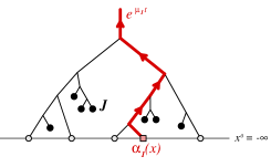
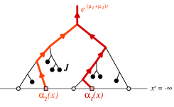
Figure 4: Exponential growth of perturbations to a classical solution.

Furthermore, this exponent is proportional to the number of points where the initial condition is perturbed. Based on this, one can easily see that the graphs with the fastest growth are those depicted in Figure 5.

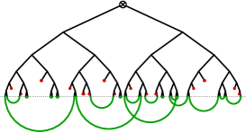
Figure 5: Graphs with the fastest growth.

The sum of all these graphs can be generated simply by exponentiating the operator in eq. (5),

$${\cal O}_{{}_{\rm{resummed}}}[J,{\cal A}_{\rm in}] = \exp\Bigg{[}\frac{{\hbar}}{2}\int d^{3}\mathbf{x}d^{3}\mathbf{y}\;{{\Gamma}(\mathbf{x},\mathbf{y})}\;\frac{\delta}{\delta{\cal A}_{\rm in}(\mathbf{x})}\frac{\delta}{\delta{\cal A}_{\rm in}(\mathbf{y})}\Bigg{]}\;\vphantom{\frac{\delta}{\delta{\cal A}_{\rm in}(\mathbf{x})}}{\cal O}_{{}_{\rm LO}}[J,{\cal A}_{\rm in}]$$ (6)

$$= \int\big{[}D{a}\big{]}\;\exp\Big{[}-\frac{1}{2\,{\hbar}}\int_{\mathbf{x},\mathbf{y}}{a(\mathbf{x})}{{\Gamma}^{-1}(\mathbf{x},\mathbf{y})}{a(\mathbf{y})}\Big{]}\;{\cal O}_{{}_{\rm LO}}[{\cal A}_{\rm in}+{a}].$$

The second line is an exact alternate representation of the action of this exponentiated operator, more suitable for a practical implementation. Indeed, it indicates that this resummation can be obtained as an average over classical solutions, obtained by superimposing Gaussian fluctuations to the LO initial condition (this resummation is known as the Classical Statistical Approximation). The function $\Gamma$ is known both in scalar theory and in Yang-Mills theory [8].

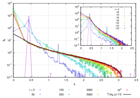
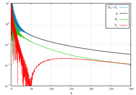
Figure 6: CSA results in scalar field theory.

Some examples of applications [9, 10, 11] of this resummation is shown in Figure 6, in the case of a $\phi^{4}$ scalar field theory (known to have unstable classical solutions due to a parametric resonance). As one can see, the particle distribution evolves towards the equilibrium one (but in this case, it is a classical distributions, of the form $T/(\omega-\mu)-1/2$), and one also observes the isotropization of the energy-momentum tensor for a longitudinally expanding system.

However, the application of the CSA with these initial conditions is hindered by a severe sensitivity on the ultraviolet cutoff (e.g., the lattice spacing). Indeed, the fluctuations added to the classical field are zero-point vacuum fluctuations, and the CSA breaks the renormalizability of the original theory by considering certain graphs but not all of them. Within quantum field theory, the Kadanoff-Baym equations (also known as the 2PI formalism) would provide a renormalizable scheme that resums the relevant contributions for thermalization. Unfortunately, its application to expanding systems has been so far limited to a proof-of-concept study [12] due to its challenging difficulties.

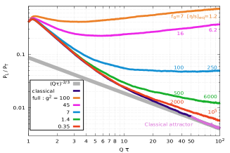
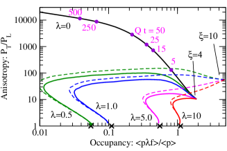
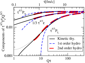
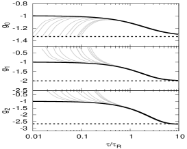
Figure 7: Kinetic theory results. Top left: isotropization in an expanding system of scalar fields [13]. Top right: isotropization in Yang-Mills theory [14]. Bottom left: comparison with hydrodynamics [14]. Bottom right: the two attractors of kinetic theory for a longitudinally expanding system [15].

A much simpler to implement alternative, that requires additional approximations (quasi-particle approximation, gradient approximation), is kinetic theory. Various studies based on solving Boltzmann equation have been performed, teaching the following insights:

• The zero-point fluctuations are crucial for the isotropization of the energy-momentum tensor in an expanding system (indeed, one may easily remove the corresponding terms in the collision kernel of the Boltzmann equation – doing so prevents isotropization).

• Isotropization is rather rapid, and the hydrodynamical behavior is observed significantly before full isotropization is achieved. Moreover, the validity of the classical approximation is much shorter than previously believed: $Q_{s}\tau_{\rm class}\ll\alpha_{s}^{-3/2}$.

• A system undergoing longitudinal expansion has only two attractors: a free-streaming attractor for times small compared to the collision time, and an isotropic attractor when the time is large compared to the collision time.

Although these findings have been obtained in the approximate framework of kinetic theory, it would be rather surprising if these qualitative behaviors were changed significantly by going to the more fundamental framework provided by the Kadanoff-Baym equations. However, to ascertain these observations, it would certainly be desirable to perform a similar study using the 2PI framework.

References

- [1] L. V. Gribov, E. M. Levin and M. G. Ryskin, Phys. Rept. 100, 1 (1983).
- [2] F. Gelis, E. Iancu, J. Jalilian-Marian and R. Venugopalan, Ann. Rev. Nucl. Part. Sci. 60, 463 (2010).
- [3] F. Gelis and R. Venugopalan, Nucl. Phys. A 776, 135 (2006).
- [4] T. Lappi and L. McLerran, Nucl. Phys. A 772, 200 (2006).
- [5] A. Krasnitz and R. Venugopalan, Phys. Rev. Lett. 84, 4309 (2000).
- [6] K. Fukushima and F. Gelis, Nucl. Phys. A 874, 108 (2012).
- [7] F. Gelis, T. Lappi and R. Venugopalan, Phys. Rev. D 78, 054019 (2008).
- [8] T. Epelbaum and F. Gelis, Phys. Rev. D 88, 085015 (2013).
- [9] T. Epelbaum and F. Gelis, Nucl. Phys. A 872, 210 (2011).
- [10] K. Dusling, T. Epelbaum, F. Gelis and R. Venugopalan, Phys. Rev. D 86, 085040 (2012).
- [11] T. Epelbaum and F. Gelis, Phys. Rev. Lett. 111, 232301 (2013).
- [12] Y. Hatta and A. Nishiyama, Phys. Rev. D 86, 076002 (2012).
- [13] T. Epelbaum, F. Gelis, S. Jeon, G. Moore and B. Wu, JHEP 1509, 117 (2015).
- [14] A. Kurkela and Y. Zhu, Phys. Rev. Lett. 115, no. 18, 182301 (2015).
- [15] J. P. Blaizot and L. Yan, Phys. Lett. B 780, 283 (2018).