Spinors, lattices, and classification
of integral Apollonian disk packings
Abstract
A parametrization of integral Descartes configurations (and effectively Apollonian disk packings)
by pairs of two-dimensional integral vectors is presented.
The vectors, called here tangency spinors
defined for pairs of tangent disks, are spinors associated to the Clifford algebra
for 3-dimensional Minkowski space.
A version with Pauli spinors is given.
The construction provides a novel interpretation to the known Diophantine equation
parametrizing integral Apollonian packings.
Keywords: Integral Apollonian disk packings, tangency spinors, Pauli spinors, integral lattices.
MSC:
52C26, 11H06, 11D09, 52C05, 51F25, 15A66.
Notation: Throughout this paper both a disk and its curvature will be addressed by the same symbol.
Introduction
Integral Apollonian disk packings are remarkable geometric objects studied by number-theorists and geometers. First of all, it might be surprising that such objects exist – arrangements of tangent disks, all curvatures of which are integers. There are infinitely many of them and identifying them is a natural task. The present paper shows that any pair of integral 2-vectors (effectively, a set of four integers , , , ) generates an integral Descartes configuration and consequently an integral Apollonian packing:
where denote the curvatures of the disks. Formally, vectors and are spinors of 3-dimensional Minkowski space. Here, they have a geometric context and are defined for any pair of tangent disks, hence are called ‘tangency spinors”. They are discussed in more detail in [6, 8, 9], and reviewed in Section 2. The above construction provides a novel interpretation to the known Diophantine equation that generates and parametrizes the integral packings [11]. As a result, a one-to-one correspondence between irreducible integral Apollonian disk packings and certain irreducible integral sublattices of (each defined by a pair of spinors as the principal basis) emerges.
And now some basic notions organized in a form that should be easy to consult. For more on the subject see [1, 2, 3, 5, 12, 15, 16, 17, 20].
-
•
A disk is an interior or the exterior of a circle. The two types of disks will be called inner and outer, respectively. The former is assumed to have a positive curvature, the latter negative.
-
•
A tricycle is a configuration of three mutually tangent disks, no pair overlapping.
-
•
A Descartes configuration is an arrangement of four mutually tangent circles. Every tricycle may be completed to a Descartes configuration in two ways.
-
•
Descartes formula (found by René Descartes in 1643) is a relation for Descartes configuration:
(1.1) where , , , and are the curvatures of the disks, i.e., reciprocals of their radii. Equation (1.1) solves Descartes problem: given a tricycle, find curvature of fourth circle tangent to the three. Due to quadratic nature of (1.1), there are two solutions to the Descartes problem for the fourth disk:
We will call them conjugated through disks . The resulting two Descartes configurations that differ by the fourth disk will also be called conjugated.
-
•
Descartes formula (1.1) may be viewed as a Diophantine equation, the integral solutions to which will be called Descartes quadruples. A Descartes disk configuration is called integral if the curvatures form a Descartes quadruple. It is irreducible if the curvatures are coprime, that is do not have a common factor, . Here is an example of a pair of conjugated Descartes quadruples:
-
•
A tricycle or Descartes configuration is everted if it contains a disk of negative curvature.
-
•
Every tricycle may be completed uniquely to an Apollonian disk packing (called simply Apollonian packing) by recursive inscribing new disks in the curvilinear triangular regions formed by the disks. If an Apollonian packing contains an integral Descartes configuration then it is integral i.e., its all disks have integral curvatures. Consequently, the integral Apollonian disk packings may be classified by the integral Descartes configurations.
-
•
A Descartes configuration or tricycle is maximal if its completion to the Apollonian packing does not contain circles of smaller curvature than those in . This definition is motivated by the fact that an Apollonian packing may be grown from any Descartes quadruple it contains. Reducing this redundancy to the maximal cases allows one to classify the integral Apollonian disk packings by maximal irreducible disk configurations.
-
•
The major disk in a disk configuration is the disk of negative or zero curvature if such exists. Its boundary is called the major circle. All integral Apollonian packings have a major circle (equivalent to the greatest among the circles).
-
•
The corona is the set of all disks in the Apollonian packing that are tangent to a given disk. The major corona is the corona at the major circle. For more on coronas see [9].
Let us also recall the theorem that defines an algorithm for generating all integral disk packings, copied here from [6]:
Theorem 1.1.
[Parametrizing formula] There is a one-to-one correspondence between the irreducible integral Apollonian gaskets and the irreducible quadruples of non-negative integers that satisfy
| (1.2) |
with constraints
| (i) | (1.3) | |||||
| (ii) |
Every solution to (1.2) corresponds to an integral Apollonian disk packing with the following quintet of the main curvatures:
The quadruples and are conjugated (see Figure 1).
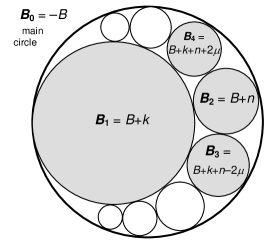
The derivation of this result was based on inversions of Apollonian strip with changing location of the point of tangency with the circle it was transformed. Conditions (1.2)–(1.3) can easily be codified into an algorithm which lists all maximal irreducible integral Descartes quadruples in an organized fashion. Table in Figure 2 shows the algorithm at work for .
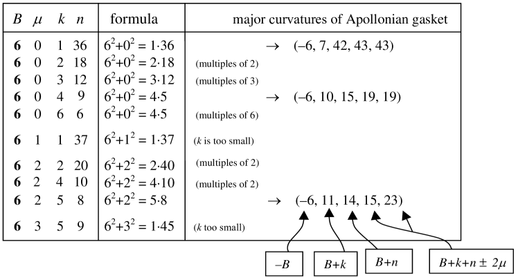
For any there are such irreducible maximal Descartes configuration and implied integral packings of the disk of curvature (on average, about of them.) An initial fragment of the resulting list is shown in Table 2. See also Figure 3. Note that, interestingly, columns and contain sums of squares.
Question: Is there a geometric picture behind the algebraic equation ?
This is were the aforementioned “tangency spinors” come into play (Section 2).
Pairs of such spinors determine Descartes configurations (Section 3).
With the help of the lattices that they define, a one-to-one parametrization of
the integral packings is achieved (Section 4).
Consequently, the family of the irreducible integral Apollonian packings
can be visualized as a dust of points in the celestial sphere,
which matches with a similar image of the corresponding lattices in the hyperbolic upper half-plane
(Section 5).
![[Uncaptioned image]](/html/2001.05866/assets/x3.png)
We finish the paper with a surprising coda. The pair of tangency spinors define a Pauli spinor, a vector in , well-known in theoretical physics. The parametrizing formula obtains a form of vanishing determinant of the Hermitian matrix defined by the Kronecker power of this spinor:
where the star denotes Hermitian conjugation. This brings the world of theoretical physics with the (1+3) space-time and associated spinors into the picture.
Spinor space for tangent disks
In his section we review briefly the notion of tangency spinor of disks. For details, proofs, and motivation see [6].
2.1 Spinor space
In the following, by the spinor space we will mean a two dimensional real vector space, which may be also emulated with 1-dimensional complex space (Argand plane), . Typical vectors are:
The space is equipped with two structures, the Euclidean inner product (“dot product’)’ and the symplectic product (“cross-product”), both with values in real numbers:
We also define ‘’symplectic conjugation”
The two structures are related:
Other identities are readily implied:
The squares are:
Interpretation via complex numbers. When the spinor space is represented by complex numbers,
then the above structures are expressed as follows:
Note that by “conjugation” we mean “symplectic conjugation” (denoted by star ). Not to be confused with “complex conjugation”, always called by its full name and denoted by the regular asterisk .
2.2 Spinors and Descartes
Definition: Let and be an ordered pair of mutually tangent disks of radii and and centered at and , respectively, in a plane identified with complex numbers, . Interpret the vector joining the centers as a complex number . The tangency spinor of the two disks is a complex number or equivalently as a 2-vector defined as
The spinor is defined up to a sign since .
Also, the spinor depends on the order of disks:
if is a spinor for , then the spinor for is
(again, both up to sign).
In graphical representation we will mark a spinor by an arrow that indicates the order of circles, and will label it by its matrix value. The geometric interpretation and motivation can be found in [6] and in Appendix A. The proofs of the main properties listed below are in [6]. For economy, capital letters will denote both circles and their curvatures.
Theorem 2.1. If is the tangency spinor for two tangent disks of curvatures and , respectively, (Figure 4, top left) then
| (2.1) |
Theorem 2.2. [curvatures from spinors] In the system of three mutually tangent circles, the symplectic product of two spinors directed outward from (respectively inward into) one of the circles is equal (up to sign) to its curvature. Following notation of Figure 4 top center:
| (2.2) |
Theorem 2.3. [mid-circle from spinors] For the situation as above, the dot product of the spinors equals the curvature of the mid-circle , i.e., the circle through the points of their tangency. Following the notation of Figure 4, top right:
| (2.3) |
Theorem 2.4. [spinor curl]. The signs of the three tangency spinors between three mutually tangent circles (Figure 4, left) may be chosen so that
| (2.4) |
Theorem 2.5.
Let , , , and be four circles in a Descartes configuration.
[A. Vanishing divergence]:
If , and are tangency spinors for pairs , and
(see Figure 4, bottom center),
then their signs may be chosen so that
| (2.5) |
The same property holds for the outward oriented spinors.
[B. Additivity]: If and are spinors of tangency for pairs and
(see Figure 4, bottom right),
then there is a choice of signs so that the sum
| (2.6) |
is the tangency spinor of .
We shall need also the following concept: Two spinors from disk and to disk are adjacent if , , and are tangent and there exists disk such that the whole quadruple forms a Descartes configuration. The same goes for reciprocal spinors, i.e., to . For instance, spinors and in Figure 6 are adjacent, while and are not.
Remark 1:
Theorem 2.5 may be viewed as a “square root of Descartes Theorem”,
since squaring the formula in a careful way reproduces Descartes formula [6].
(The two version of this theorem are equivalent and differ by a sign of one spinor and geometric interpretation).
Remark 2:
It should be noted that the “divergence” and the “curl” theorems have local character.
Extending the spinor vector field to the Apollonian disk packing cannot be done consistently
due to topological obstruction, quite like the non-existence of smooth non-vanishing vector field on a sphere.
Remark 3: the name tangency “spinor” is justified by the fact that
it represents spinor for the (1+2)-dimensional Minkowski space
in which Pythagorean triples are null-vectors (metaphorically, photons)
[7].
Consequently, they behave like electron spins known in quantum physics:
rotating a configuration of circles around by causes the spinors rotate by only ,
i.e., they change the signs.
It takes two full rotations of a circle configuration to bring the spinors to their original signs.
Notation: A spinor from disk to will be denoted sometimes as
Clearly, (or when represented as complex numbers).
Integral Descartes configurations from spinors
Proposition 3.1: Suppose two tangent disks of positive curvatures and are inscribed in a disk of negative curvature (see Figure 5). Suppose the tangency spinors are
Denote . Then the following are true
| (3.1) |
Moreover, the following quadruples satisfy Descartes formula
where
Proof: Direct consequence of Theorems 2.1–2.5 of the previous section. Indeed, one has
Denote and invert the equations to get the claim. ∎
Note that the scalar may be defined by any pair of the above spinors:
where . Indeed, , and similarly for the second equation.
Proposition 3.2: Any two integral vectors and determine an everted Descartes configuration with integral curvatures defined
| (3.2) |
Consequently, the implied Apollonian disk packing is also integral. Moreover, for any vector
| (3.3) |
there is a disk in the major corona of the Apollonian packing with the curvature
| (3.4) |
If and are two such linear combinations and
then the disks
form a tricycle.
Each of (3.2) is a special case of (3.4).
Proof: This follows by reversed reading of the equations (3.1) of
the previous proposition, supplemented with Theorems 2.2 and 2.5B:
start with given spinors and build the Descartes quadruple.
Note that setting the negative sign in assures the
that disk is the major disk in a everted configuration.
In other words, define ,
and then
must satisfy the Descartes formula. Consult Figure 6 for clarification. Appendix A provides concrete coordinates for the disks, given the tangency spinors. ∎
Now for some examples.
Example 1. Consider the following two spinors:
Then
Hence the two Descartes configurations (for different sign in ) are
as illustrated in Figure 6. The figure shows also the Apollonian packing implied by the above Descartes configurations.
Example 2: Let us try another choice of integral vectors:
Calculate
Hence the curvatures are determined and the two Descartes configurations are
One may identify these disks in Figure 7 (green disks in the left lower region). Different Descartes quadruples may give the same Apollonian disk packing. This example is to show that a random choice of integral spinors does not necessarily lead to a maximal Apollonian packing. But their appropriate linear combination will give the principal spinors and the corresponding maximal Descartes configuration:
Example 3: Let us see what happens when one chooses two non-adjacent spinors in the Apollonian packing in Figure 6.
Since the spinors build a different Apollonian packing. The implied Descartes configuration is
which will produce a different Apollonian packing.
3.1 Parametrizing formula interpreted
The Descartes formula may be derived from the spinor theorems 2.1–2.5 (see [6]). One may start with the Pythagorean Theorem , multiply it by absolute values of two vectors in to get a known vector formula shown below. Next, interpret the vectors as two adjacent spinors to get the following correspondence:
| (3.5) |
This formula is valid for any tricycle.
But if one of the disks is assumed to be outer (i.e., of negative curvature),
one may readily recognize in the above equation the terms
of the parametrizing formula of Theorem 1.1, as shown in the above box.
Suddenly we have a spinor interpretation of the algebraic terms of the parametrizing formula.
Terms and are simply the norms squared of spinors and therefore they must be sums of squares.
Term turns out to be the inner product of spinors, and as such it represents the mid-circle .
Remark: To see that Equation (3.5) is equivalent to Descartes’ formula,
replace the vector products with the expressions in terms of curvatures from Proposition 3.2 to (3.5) to get
| (3.6) |
which reduces in a few steps to the known standard form (1.1).
3.2 Remark on Brahmaputra-Fibonacci identity
From the number-theoretic point of view Equation (3.5) may be interpreted as an instance of Brahmaputra-Fibonacci identity:
Thus the (3.5) provides (1) a vector interpretation of the Brahmaputra-Fibonacci identity, and (2) a geometric interpretation in terms of disks. Moreover, it is clear that it is a form of Pythagorean Theorem!
| (3.7) |
Remark:
Note that the cross-product is defined only in dimensions 2, 3 and 7
(the last two due to the existence of quaternions and octonions)
hence the Brahmaputra-Fibonacci identities have the corresponding generalized versions.
Corollary: The meaning of of the parametrizing formula is extended:
where denotes curvature of the circle
through the points of tangency of circles 1,2, and 3.
Remark: If the circle is to small (or, too big), the spinors and fail to be principal because the respective circles are too “crumbled” together, too small to like in Figure 7.
Lattices
Here we review some basic facts about lattices, restricted to the case of two dimensions [13, 14, 19]. The two-dimensional integral lattice is called Diophantine plane or the standard integer lattice.
By an integral lattice we will understand any 2-dimensional sublattice of , i.e., a -module generated by two linearly independent vectors and of the Diophantine plane:
| (4.1) |
Matrix whose columns are made by the basis vectors, , allows one for abbreviated description of the lattice:
The primitive cell for a basis , is the region
Placing a copy of the primitive cell at every lattice point produces a tiling of the plane. Figure 9 shows two choices of basis generating the same lattice and the corresponding two different primitive cells. The discriminant of a lattice (called also the “determinant” of the lattice) is defined as the area of the primitive cell
It does not depend on the choice of basis. Two bases define the same lattice if they are the image one of the other via unimodular matrix, i.e. transformation from the group
A basis is called principal if it consists of the shortest vectors of the lattice. One of the bases in Figure 9 is principal. Note that such a reduced basis may be always chosen so that the basis vectors make a right or acute angle:
Indeed, you may always replace one of the basis vectors by its negative, as it has the same length, tochange the sign of the above inner produc. We shall include this to the definition; A basis is principal if it is ordered, reduced and makes an acute angle:
To find a principal basis for a given lattice, one performs a basis reduction process.
Start with any basis
and replace the longer vector, say , by to
get a new basis .
Repeat until such a move does not reduce the size of vectors any more.
This is an analogue of the Euler’s algorithm for computing the greatest common divisor.
An obvious (in 2D case) characterization follows:
a basis of a lattice is Lagrange-Gauss reduced
if
for every .
In the case of 2-dimensional basis this coincides with the principal basis.
We shall call two integral lattices similar if one may be obtained from the other by
any composition of rotation, reflection and dilation. Figure 10 shows an example of three
mutually similar lattices. (The numbers denote the discriminant of the lattices.)
For every integer there exist a finite number of integral lattices of discriminant . Figure 11 shows them for , and .
We shall introduce yet another term: The 2-dimensional Euclidean mosaic is the set of vectors (points) in the Diophantine plane whose components are coprimes:
Equivalently, it is the orbit of via the action of the unimodular group , the group of matrices of determinant equal to . Euclidean mosaic is not a lattice, as it is not a group (see Figure 12). Mosaic of a lattice is defined analogously as the subset
The reason for introducing this term is the fact that due to Theorem 2.5B, the spinors of a given corona form a mosaic in the lattice defined by spinors.
4.1 Lattices and Apollonian packings
With the language of lattices, we may now restate the content of Proposition 3.1 and 3.2 as follows:
Proposition 4.1.
The corona spinors in an Apollonian packing
form a mosaic in the lattice defined by any pair
of the adjacent spinors in the corona.
Proof: Any two adjacent spinors in the corona
determine a lattice .
By Theorem 2.5B, any other spinor in the corona is a linear combination of the two,
hence is an elements of the same lattice.
But since the combinations involve coprime coefficients, they will make a subset of the lattice,
coinciding with its Euclidean mosaic.
∎
The very existence of the lattice allows one to find its principal basis – two shortest vectors in the lattice –
through the reduction process described the previous subsection.
They point to (or from) the greatest circles in the corona, and consequently
indicate the maximal Descartes configuration in the Apollonian packing.
Thus we get a connection with the parametrizing formula of Theorem 1.1,
together with the interpretation of , , and given in (3.5),
now applied to the principal spinors.
This establishes also uniqueness of the classification
via the lattices up to similarity.
Indeed, rotations and reflections do not change the values
of , and , while scaling would
lead to quadruples of curvatures with a common divisor.
In conclusion, the list of lattices, as illustrated in Figure 11
is equivalent to the classification of the irreducible Apollonian packings.
Remark 1:
To achieve uniqueness of the spinor representation of lattices,
we may demand an extended list of conditions:
(1) — vector is shorter than .
(2) — vector is in the first quadrant, close to the x-axis.
(3) — vector is in the first or second quadrant.
(4) — the vectors form an acute or right angle.
Remark 2:
The above is true for any corona on any disk.
Only when our attention was on classification of the integral Apollonian packing,
we concentrate on the outer disk with negative curvature.
Proposition 3: Every tangency spinor in the Apollonian packing is a linear combination
where ,
and and is a pair of adjacent spinors at any disk in the packing.
In particular, if and are integral, so are all spinors in the packing.
Proof: This is a simple consequence of Theorems 2.4 and 2.5, which allow one to extend the values of spinors throughout the packing.
4.2 Derivation of the constraints
The conditions on , and for the parametrizing formula in Theorem 1.1 obtain a simple geometric justification when considered in the lattice context. Recall that two spinors that determine a lattice may not correspond to the maximal Descartes configuration. But they may be adjusted by the reduction process, i.e., a sequence of mutual subtraction / additions, until none can be replaced by a shorter one.
Proposition 4.1:
Principality of spinors defining a Descartes configuration implies the conditions (1.3)
of Theorem 1.1.
Proof: Let us assume that and are two spinors forming a principal basis of the lattice defining the corona of an Apollonian packing. Recall notation and , and assume the order
| (4.2) |
(or ). Principality implies that the longer vector cannot be replaced by to make the basis vectors shorter. In other words:
Squaring both sides,
leads to
| (4.3) |
Now, this and the assumption imply
and, after cancellation,
In other words, , or
This implies . Multiplying both sides by we get
| (4.4) |
In terms of notation of (3.5):
the above properties (4.2), (4.3), and (4.4), translate into:
as stated. ∎
Remark: Intuitively, condition is equivalent to the geometric requirement that the mid-circle be not too small; otherwise, a circle greater than any of the two, or will be possible in the corona of .
4.3 Curious examples of Apollonian strip and of unbounded “golden” packing
A few examples that work, even if they seem degenerated.
Example 4: Interestingly, the initial spinors do not need to be linearly independent to determine an Apollonian packing. Start with
Calculate , , , and . The two complementary Descartes configurations are therefore
One readily recognizes that they generate the Apollonian strip, see Figure 13. The integral sublattice is here one-dimensional, .
Example 5: One does not even need a requirement of non-zero vectors! For the sake of an experiment, let us try
Then , , , and , and the two Descartes configurations are
which, as in the previous example, may be completed to the Apollonian strip. One should consider this case as the reduced, principal, basis of Example 4. Tangent spinor connects the straight lines (the half-spaces), considered as tangent at infinity, see Figure 13. Clearly, this one-dimensional lattice needs to be included into the list of lattices corresponding to the integral Apollonian packings.
Example 6: Start with
where is the golden ratio. Then the two Descartes configurations are
As shown in [10], this corresponds to an unbounded Apollonian packing which does not contain a disk of minimum positive curvature (see Figure 14). Note that that the process of reduction would be a never-ending task:
Celestial sphere, modular plane, and Pauli spinors
In this section we will sent the following observation:
Proposition. The celestial sphere image of irreducible Descartes quadruples understood as vectors in the Minkowski space coincides with the corresponding lattices represented in the hyperbolic half-plane.
Below we explain and prove this observation.
5.1 Celestial sphere
Descartes’ formula may be written in terms of a quadratic form:
| (5.1) |
The matrix of this quadratic form defines a pseudo Euclidean norm of signature , the norm of Minkowski space.111It is however not the Minkowski space of circles as introduced in [5], but rather its dual space. The above equation implies that the Descartes quadruples may be viewed as vectors in the Minkowski space that lie on the null cone, known as the light cone to physicists.
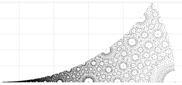
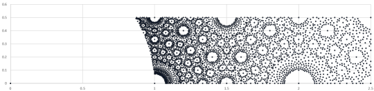
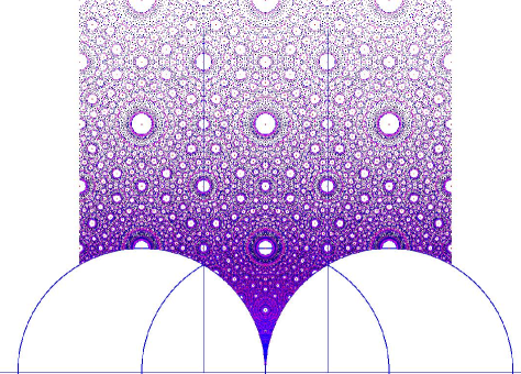
We may think of them as “photons” coming from distant stars, and present them as points in the sky – the celestial sphere. A sphere may in turn be stereographically projected on the 2D plane. The result of this process is presented in Figure 15 for quadruples with the value of from 0 to 300 (more than 12000 points).
Let us trace the steps. First, diagonalize the quadratic form of Equation (5.1). Here are two of many possible diagonalizations of 5.1:
Descartes formula in the diagonalized coordinates becomes
(as it is easy to check.) Equation defines a three-dimensional space in , and its intersection with the light cone defines a sphere in it. It is called the celestial sphere. The Descartes quadruples may be projected along the rays onto this sphere.
Obviously, . Now, we can perform the stereographic projection from this sphere onto plane via
where the first pair follows the projection from the North pole, while the second from the South pole.
Figure 15 shows the latter.
The former would gives an unbounded dust of points shown in Figure 16,
extending infinitely to the right.
5.2 The modular space of lattices
There is a standard way to visualize the space of all 2D lattices in a complex plane as follows (see e.g., [19]): Identify the lattice plane with complex plane. The basis vectors of a lattice are now two complex numbers . Consider the map:
| (5.2) |
This map corresponds to scaling and rotating the lattice so that vector becomes 1. Vector preserves the information of the ratio of the length of the vectors and their mutual angle.
If one applies this to the principal basis, its complex representation lies in the fundamental domain of the modular tessellation of the Poincaré half-plane (the shaded region in Figure 17), more precisely, in the region defined by , , . The other bases fall in the other tiles of the Dedekind tessellation and are images of the principal point via Möbius action
where the matrix is a group element of the unimodular group .
Let us apply this to the lattices representing the Descartes configurations with the principal spinors and :
Thus
| (5.3) |
With the help of software, we can produce an image that turns out quite similar to the one in Figure 16.
5.3 Proof of the Proposition 5.1
The puzzle of similarity of the patterns in the two images, the one obtained via celestial sphere and one in the hyperbolic plane, may easily be explained. One of the diagonalizations of the Descartes formula is:
Associate , , , . Substituting these entities to the celestial sphere coordinates gives:
and consequently
| (5.4) |
which coincides with the formula for the projection from the North projection of the celestial sphere (5.3). Hence the obtained image must coincide with the belt-like right half of the fundamental region of Figure 17.
The stereographic projection of the celestial sphere from the south pole S requires a sum in the denominator of (5.4) and resolves as follows:
| (5.5) |
( instead of in the denominator.) The resulting image is illustrated in Figure 15. Now, for the complex plane representation of lattices, one obtains the matching image by mapping the fundamental domain to the triangle-like region underneath by the unimodular transformation:
(after using ). Reflection will map the point to the right side of the triangular region, with coordinates
which coincides with the formulas for projection of the celestial sphere projected onto the plane from the south, (5.5).
5.4 Unification: Pauli spinors from tangency spinors
The tangency spinors are spinors for the 3-dimensional space with Minkowski quadratic form of signature (1,2). It has been a somewhat metaphorical use of the term native to mathematical physics of (1+3)-dimensional spacetime for objects in 2-dimensional geometry. But now, by some magical turn, the two worlds merge when we represent a pair of tangency spinors as a single Pauli spinor:
Consider the following map . First, view the tangency spinors back as the complex numbers: (same for spinor ). Next, define a “metaspinor”
(which is the usual Pauli spinor, known in the context of (1+3)-Minkowski space). Now, consider a Hermitian matrix constructed from this spinor:
where the star denotes the Hermitian conjugation: transposition and complex conjugation. The tensor product may be realized as the Kronecker product.
Proposition: The connection between the tangency spinors and the curvatures, and the parametrizing formula (and consequently the Descartes formula) can be expressed in a single statement:
Proof: We get
Since the matrix is of rank 1, its determinant vanishes automatically. This immediately implies .
Remark 1: The above parallels the correspondence well known in theoretical physics, where vectors in Minkowski space-time are mapped to the space of Hermitian matrices:
The Lorentz norm is represented now by a determinant:
In particular, any vector (Pauli spinor) defines a null-vector (“photon”) by setting , which may be understood as the Kronecker product. Since it is of rank 1, its determinant is vanishing, and so is the norm of the Minkowski vector it defines. Once we view Descartes quadruples as null vectors in the Minkowski space, we may evoke these standard means from physics, including the Pauli spinors, the elements of . This is where one may use Pauli matrices:
which allow one to express a vector as a Hermitian matrix via the map:
Remark 2: Some additional formulas for matrix follow easily:
5.5 Hopf fibration and the projective spinor space
The stardust may also be reproduced in terms of the Pauli spinors. Indeed, consider the following chain of maps
The first map in the chain is a normalization of vectors by the standard Hermitian norm in . The result is a three-dimensional sphere in . The second map is the Hopf fibration of the 3D sphere over 2D sphere , The composition of these maps is simply the projection map from to the projective space . In such a context, is known in quantum physics as the Bloch sphere. The last map is the usual stereographic projection of a 2D sphere to the plane. As it is easy to see, the composition of these maps abbreviates to
which is exactly of the same form as the maps considered in the previous subsections, cf., (5.2). (Clearly, the zero vector needs to be excluded from these maps.)
Summary
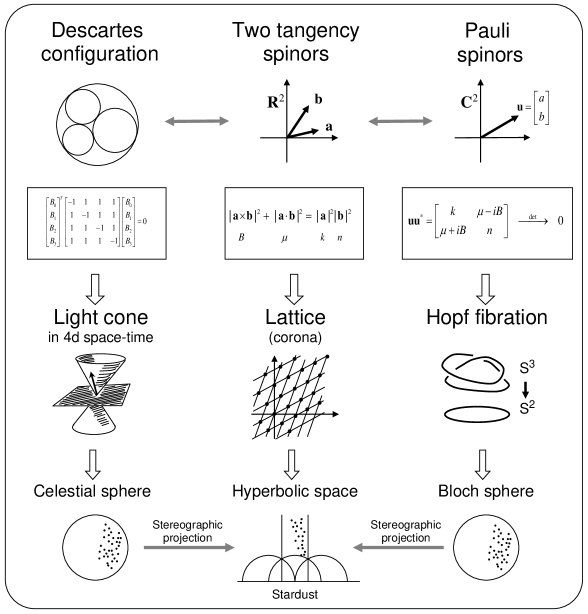
1. The relations between the tangency spinors and Descartes configurations discussed in the present paper are summarized in the following diagram. The top row concerns spinors, the bottom the disks. Restricting the objects to integral curvatures leads to the parametrization of the irreducible packings.
Two arbitrary 2D integral vectors and define an integral tricycle, which, when extended, results in an integral Apollonian disk packing . But they also define a lattice in the spinor space via linear combinations. One may find the principal basis of this lattice; clearly . There are two benefits of this finding:
-
1.
Vectors relate directly to the terms of the parametrization theorem for Apollonian disk packings and explain their meaning.
-
2.
The principal spinors point to the maximal tricycle (and maximal Descartes configuration)in the Apollonian packing.
Other circles in the boundary corona in
are obtainable via linear combinations of the basis vectors.
2. Somewhat unexpectedly, there is a deeper level on which the concepts are related. The results may be reorganized with the help of a number of ideas known from theoretical physics, like Pauli spinors of quantum mechanics or celestial sphere from the theory of relativity. Also, the family of the integral Apollonian packings finds a geometric image as points in celestial sphere, Bloch sphere, or hyperbolic space. This is summarized in Figure 19.
3. On the lighter side, as a final remark, let us notice that the two main spinor equations lead to two different geometric extensions:
The first connection is explained in [8]. Stripping its geometric content, we get a method of obtaining integral Descartes configurations (and consequently integral Apollonian disk packings) from four arbitrary integers as follows.
Let and be arbitrary integral vectors in . Then the following values satisfy the Descartes equation (1.1) for three tangent inner disks and the fourth one of the two conjugated disks or :
| (6.1) |
Compare it with the content of the present paper:
| (6.2) |
On the other hand, the spinor - Descartes quadruple can also be given a simple geometric interpretation in terms of areas of tiles, as shown in Figure 20. The parallelogram is that of the fundamental cell. The curvatures of the greatest disk in the implied Descartes configuration are the sums of the dark (red) region and one of the two lighter squares (yellow). The next two (shown aside) are based on the two diagonals of the parallelogram.
Note on software: Most of the figures were made with Tikz [21].
Appendix A
The geometric interpretation and motivation follows. Every disk in the Cartesian plane may be given a symbol, a fraction-like label that encodes the size and position of the disk: the curvature is indicated in the denominator while the positions of the centers may be read off by interpreting the symbol as a pair of fractions [5].
The numerator, called the reduced coordinates of the a disk’s center, is denoted by dotted letters . Unbounded disks extending outside a circle are given negative radius and curvature. Two tangent disks in a plane define a triangle with sides as follows [7, 6]:
| (6.3) |
where (see Figure 21). The actual size of the triangle in the plane is scaled down by the factor of (gray triangles in Figure 21). The symbols in some disk packing are integral, then so are the triples . Recall that Pythagorean triangles admit Euclidean parameters that determine them via the following prescription:
(see, e.g., [18, 22]). As explained in [7], Euclidean parameters can be viewed as a spinor, a vector of . Equivalently, viewing the spinor as a complex number the above relations is defined by squaring:
with .
We extend this map to arbitrary oriented triangles, not necessarily integer.
The emergence of the tangency spinor for a pair of tangent disks is summarized in Figure 21.
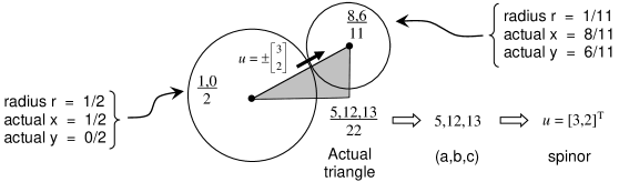
The curvatures are the numbers in the denominators of the “symbols” inscribed into the disks. The numerator numbers in the fractions code the positions of the disks in the euclidean plane and are of no concern for us here; they are explained in Appendix A.
Drawing the Apollonian packing from the defining spinors
It is easy to define uniquely the spinor given full data on the circles. But the reverse process can be done up to translations.
Proposition A.1: Let us assume that the main circle, the boundary of the outer disk of negative curvature is located at the origin:
Let be a disk in the major corona, the corona of , and let be a spinor
(in the graphical representation it is drawn as if leaving the packing), Then the position and the radius of the disk are:
In terms of the disk symbol:
Proof: This is a simple consequence of the definition of the spinor for two disks of radii and , respectively. If viewed as a complex number, it defines the vector distance between the centers of two circles and as . Hence, if the position of disk is , the position of circle is . A difference instead of sum must be used for the opposite spin . Apply it to the situation described in the proposition to get the result.
Another question is how to construct spinors given only curvatures of the disks.
Proposition: For any choice of three curvatures of three tangent disks, , with , there exists a spinor description, namely
The numerator in the second entry of may be replaced by , where is a solution to the Descartes problem for the given three disks. Its value coincides with the curvature of mid-circle .
Appendix B: the symmetry group aspect
A few words on the group symmetries that pertain to the Descartes configuration and the corresponding spinor structure are in order. The mutual relations are displayed in the diagrams that follow. The Lorentz group acting on the Descartes configurations will permute them. The discrete subgroup carries integral Descartes configurations to likewise ones. The Pauli spinors transform by the corresponding elements of the group .
The first diagram has a similar content, except it concerns a single tangency spinor originating from a Pythagorean triangle. The dashed line in the first diagram indicates the Euclidean parametrization. In the second, the Pauli spinor describing a Descartes configuration.
Pythagorean triples and Euclid’s parametrization
Physics, relativity, space-time
Legend
— Group acting on set ,
— Group acting on set ,
— two-by-two Hermitian matrices over
— two-by-two traceless Hermitian matrices over
— two-by-two Hermitian matrices over of determinant equal to 0
— two-by-two real symmetric matrices
Acknowledgments
The author would like to express his special thanks to Philip Feinsilver for very useful comments and encouragement. His effervescent attitude to mathematical explorations is priceless.
References
- [1] Elena Fuchs, Katherine E. Stange, Xin Zhang, Local-global principles in circle packings, Compositio Math. 155 (2019) 1118-1170.
- [2] Ronald L. Graham, Jeffrey C. Lagarias, Colin L. Mallows, Allan R. Wilks and Catherine H. Yan, Apollonian circle packings: geometry and group theory I. Apollonian group, Discrete & Computational Geometry 34 (2005), 547–585
- [3] Ronald L. Graham, Jeffrey C. Lagarias, Colin L. Mallows, Allan R. Wilks and Catherine H. Yan, Apollonian circle packings: number theory, J. Number Theory 100 (2003), 1–45.
- [4] Jerzy Kocik, Proof of Descartes circle formula and its generalization, clarified (arXiv:0706.0372).
- [5] Jerzy Kocik, A matrix theorem on circle configuration, (arXiv:1910.09174).
- [6] Jerzy Kocik, Spinors and Descartes configurations of disks, (arXiv:1909.06994).
- [7] Jerzy Kocik, Clifford algebras and Euclid’s parameterization of Pythagorean triples. Adv. Appl. Clifford Al. 17 (2007), 71-93.
- [8] Jerzy Kocik, Tessellations and Descartes disk configurations, (arXiv:1909.09941)
- [9] Jerzy Kocik, Apollonian coronas and a new Zeta function (arXiv:1909.09941)
- [10] Jerzy Kocik, A note on unbounded Apollonian disk packings (arXiv:1910.05924)
- [11] Jerzy Kocik, On a Diophantine equation that generates all integral Apollonian gaskets, ISRN Geometry, 348618 (2012)
- [12] Jeffrey C. Lagarias, Colin L. Mallows and Allan Wilks, Beyond the Descartes circle theorem, Amer. Math. Monthly 109 (2002), 338–361. [eprint: arXiv math.MG/0101066]
- [13] L. Lagrange, Recherches d’arithmétique. Nouv. Mém. Acad. (1773)
- [14] Henry McKean and Victor Moll, Elliptic Curves: Function Theory, Geometry, Arithmetic, Cambridge University Press, (1999)
- [15] Zdzisław A. Melzak, Infinite packings of disks. Canad. J. Math. 18 (1966), 838–853.
- [16] S. Northshield, “On integral Apollonian circle packings,” J. Number Theory, 119(2), 171-193 (2006).
- [17] Indu Satija, “A tale of two fractals: the Hofstadter butterfly and the integral Apollonian gaskets,” The European Physical Journal, Special topics, 225, 2533-2547 (2016)
- [18] Wacław Sierpiński, Pythagorean triangles, The Scripta Mathematica Studies, No 9, Yeshiva Univ., New York, 1962.
- [19] Jean-Pierre Serre, A Course in Arithmetic, Springer, 1996 printing.
- [20] Fredric Soddy, The Kiss Precise. Nature 137 (1936), 1021.
-
[21]
Till Tantau,
The TikZ and PGF Packages,
Manual for version 3.0.0,
http://sourceforge.net/projects/pgf/, 2013-12-20. - [22] Olga Taussky-Todd, The many aspects of Pythagorean triangles, Lin. Alg. Appl., 43(1982):285–295.
- [23] G.T. Williams and D.H. Brown, A family of integers and a theorem on circles, Amer. Math. Monthly 54 (1947), no 9, 534–536.