Solar System objects observed with TESS – First data release: bright main-belt and Trojan asteroids from the Southern Survey

Abstract

Compared with previous space-borne surveys, the Transiting Exoplanet Survey Satellite (TESS) provides a unique and new approach to observe Solar System objects. While its primary mission avoids the vicinity of the ecliptic plane by approximately six degrees, the scale height of the Solar System debris disk is large enough to place various small body populations in the field-of-view. In this paper we present the first data release of photometric analysis of TESS observations of small Solar System Bodies, focusing on the bright end of the observed main-belt asteroid and Jovian Trojan populations. This data release, named TSSYS-DR1, contains 9912 light curves obtained and extracted in a homogeneous manner, and triples the number of bodies with unambiguous fundamental rotation characteristics, namely where accurate periods and amplitudes are both reported. Our catalogue clearly shows that the number of bodies with long rotation periods are definitely underestimated by all previous ground-based surveys, by at least an order of magnitude.

1 Introduction

The Transiting Exoplanet Survey Satellite (Ricker et al., 2015, TESS) has successfully been launched on April 18, 2018 and after commissioning, started its routine operations on July 25, 2018. During the first two years of its primary mission, TESS observations are scheduled in terms of “TESS sectors” (or simply, sectors) where each sector corresponds to roughly 27 days of nearly continuous observations (in accordance with two orbits of TESS around Earth, with a spacecraft orbit in 1:2 mean-motion resonance with the Moon). The first year of observations ended on July 18, 2019, after completing the 13th sector (S13). Throughout these 13 sectors, TESS observed the primary fields on the Southern Ecliptic Hemisphere, covering the sky from the ecliptic latitude of $\beta$ $\approx$ -6^∘, down to the southern ecliptic pole. This coverage is attained by four wide-field cameras, each camera having a field-of-view (FoV) of $24^{\circ}\times 24^{\circ}$ and the gross FoV is equivalent to a nearly contiguous rectangle in the sky, with a size of $96^{\circ}\times 24^{\circ}$. The individual camera FoVs are also identified by the camera numbers and, according to the survey design, Camera #4 continuously starred at the southern ecliptic pole while Camera #1 scanned the subsequent fields just south from the ecliptic plane. The cadence of TESS observations is $30$ minutes in the so-called full-frame image (FFI) mode while pre-selected sources are observed with a cadence of $2$ minutes (hence, this mode is also called “postage stamp” mode). These two modes are also referred to as long cadence and short cadence observations: for TESS, long cadence also implies that the whole CCD frame is retrieved.

This mission design allows us to observe Solar System objects during the primary mission, even considering the fact that the ecliptic plane is avoided by $\sim 6$ degrees. At first glance, objects with an inclination higher than $\sim 6$ degrees are expected to be observed, but due to the $\sim$1 AU distance of TESS to the Sun and the semi-major axis range of $2.1-3.3$ AU for the main-belt asteroids, also considering their non-zero eccentricities, thousands of objects with a few degrees of inclination are also possible to be observed with the aforementioned spacecraft attitude configuration. This limit of $6^{\circ}\lesssim i$ is more strict for distant objects, such as Centaurs or trans-Neptunian objects.

According to earlier simulations (Pál, Molnár & Kiss, 2018), one can expect good quality photometry of moving targets down to $V\lesssim 19\,{\rm mag}$ with a time resolution of $30$ minutes corresponding to the data acquisition cycle of the TESS cameras in full-frame mode. Although the cadence for the postage stamp mode frames would allow a similar precision down to the brighter objects (i.e. $V\lesssim 16\,{\rm mag}$), the corresponding pixel allocation would be too expensive. In this aspect, TESS short cadence observations are analogous the Kepler/K2 mission (Borucki et al., 2010; Howell et al., 2014) and similarly, only pre-selected objects could be observed in this mode (Szabó et al., 2015; Pál et al., 2015). Specifically, one should allocate roughly a thousand pixel-wise stamp if observations for a certain object are required. The rule-of-thumb for the apparent tracks of main-belt asteroids on long cadence TESS images is the movement of $\approx 1\,{\rm pixel}/{\rm cadence}$ (see also Fig. 2 in Pál, Molnár & Kiss, 2018). Of course, NEOs and trans-Neptunian objects could have apparent speeds which are larger and smaller, respectively.

The yield of such a survey performed by TESS is a series of (nearly) uninterrupted, long-coverage light curves of Solar System objects – like in the case of previous space-borne studies mentioned below. From these light curves, one can obtain fundamental physical characteristics of the bodies such as rotation periods, shape constraints and signs of rotating on a non-principal axis - with a much lesser ambiguity than in the case of ground-based surveys. This ambiguity is mainly due to the fact that ground-based photometric data acquisition is interrupted by diurnal variations – which yield not just stronger frequency aliasing but higher fraction of long-term instrumental systematics. In addition, the knowledge of rotation period helps to resolve the ambiguity of rotation and thermal inertia (see e.g. Delbo et al., 2015) in thermal emission measurements of small bodies. Further combination of spin information with thermal data (see e.g. Müller et al., 2009; Szakáts et al., 2017; Kiss et al., 2019) can therefore be an important initiative.

This paper describes the first data release, TSSYS-DR1 of the TESS minor planet observations, based on the publicly available TESS FFI data for the first full year of operations on the Southern Hemisphere. The structure of this paper goes as follows. In the next section, Sec. 2 we describe how the objects were identified and what kind of object selection principles are available for a mission like TESS. In Sec. 3 we discuss the main steps of the data reduction and photometry, emphasizing the importance of differential image analysis. Sec. 4 summarizes the structure of the available data products while in Sec. 5 we make a series of comparisons with existing databases aiming to collect photometric data series for small Solar System bodies. Our findings are summarized in Sec. 6.

2 Object selection

Regarding to the identification and querying Solar System objects on TESS FFIs, one can ask two types of questions:

• When and by which Camera/CCD was my target of interest observed?

• Which objects were observed by a certain Camera/CCD during a given sector?

We can also connect these questions to the K2 Solar System observations. Namely, the first question is related to the computation of the pixel coverage of an asteroid track, as it was done in the case of K2 mission while observing pre-selected objects (see e.g. Pál et al., 2015; Kiss et al., 2016; Pál et al., 2016) and the second question is related to the observations of serendipitous asteroids crossing large, contiguous K2 superstamps (Szabó et al., 2016; Molnár et al., 2018).

In order to identify the objects which were observed by a certain Camera/CCD during a given sector, we followed a similar approach as it was done in our K2 asteroid studies (Molnár et al., 2018; Szabó et al., 2016) and in the case of simulations of TESS observations (Pál, Molnár & Kiss, 2018). Our solutions are based on an off-line tool called EPHEMD, providing a server-side backend for massive queries optimized for defining longer time intervals and larger field-of-views within the same call (see Pál, Molnár & Kiss, 2018, for more details). In fact, the catalogue presented in this paper is retrieved by simply executing EPHEMD queries on per-CCD basis for each sectors. Due to the dramatic decrease of the asteroid density at higher ecliptic latitudes, in this catalogue (DR1) we included only the observations from Camera #1.

Table 1: Quality flags and bits for the individual light curve data points. The data point flags are interpreted in a bitwise logical-or combination of these individual flags. The bit positions between 0 and 11 (values from 1 to 2048) are inherited from the FITS headers of the calibrated FFI data products, in accordance with the TESS Science Data Products Description Document(Tenenbaum & Jenkins, 2018). The bit positions from 12 to 14 (mask values from 4096 to 16384) are specific for this particular data release and might be altered in the future. Note that bits at the position 1, 6, 8 and 9 (having a description in parentheses) are not used in the TESS FFI data products.

Bit position	Value	Description
0	1	Attitude Tweak.
1	2	(Safe Mode.)
2	4	Spacecraft is in Coarse Point.
3	8	Spacecraft is in Earth Point.
4	16	Argabrightening event.
5	32	Reaction Wheel desaturation Event.
6	64	(Cosmic Ray in Optimal Aperture pixel).
7	128	Manual Exclude. The cadence was excluded because of an anomaly.
8	256	(Discontinuity corrected between this cadence and the following one.)
9	512	(Impulsive outlier removed before cotrending.)
10	1024	Cosmic ray detected on collateral pixel row or column.
11	2048	Stray light from Earth or Moon in camera FOV.
12	4096	Formal photometric noise exceeds the threshold of $0.5$ magnitude.
13	8192	Point rejected due to the presence of unexpected histogram region.
14	16384	Manual removal of an outlier point.

Original
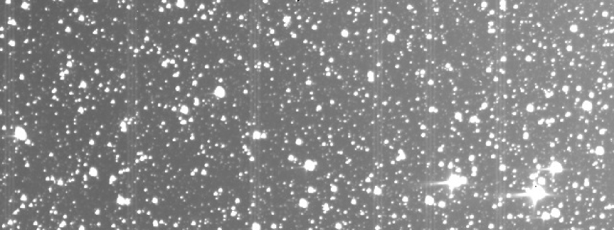
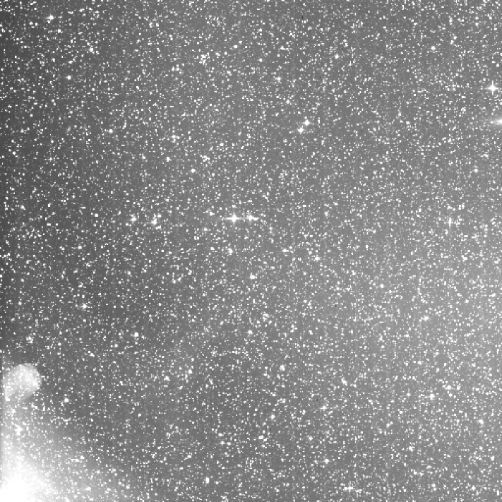
Background difference
Background variations removed
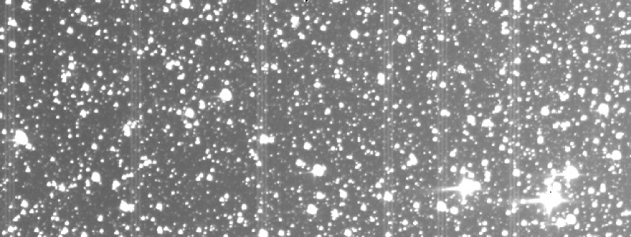
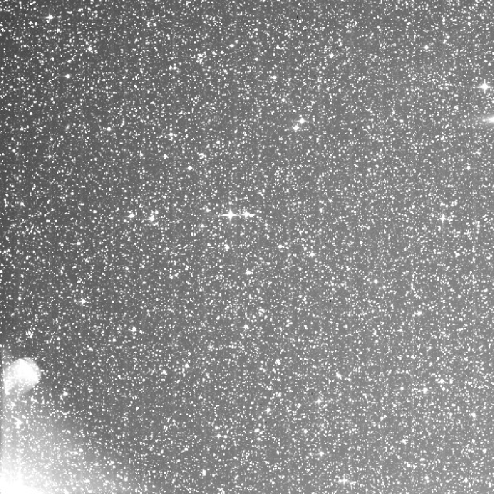
Simple difference
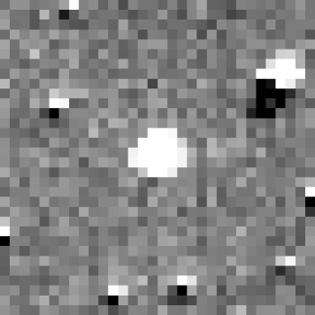
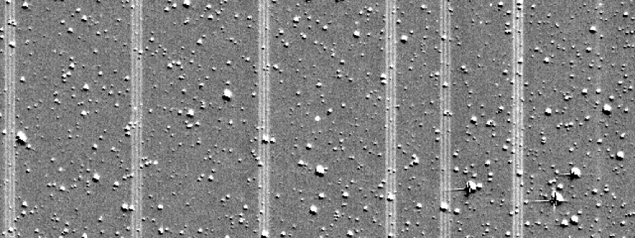
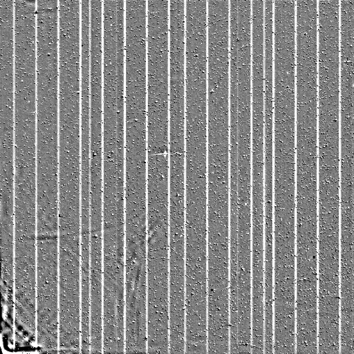
Convolution & difference
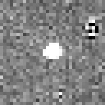
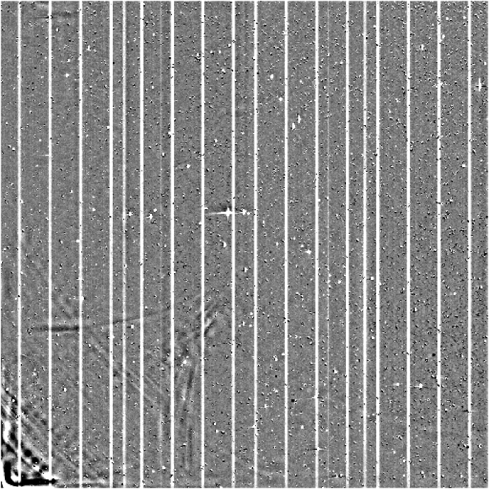
Stripes removed

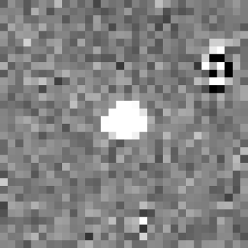
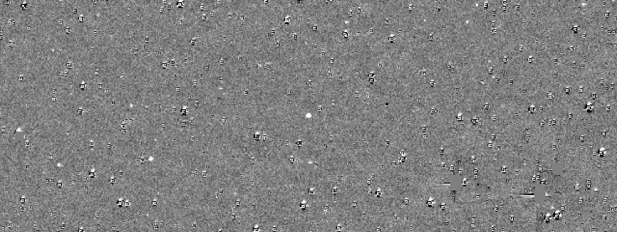
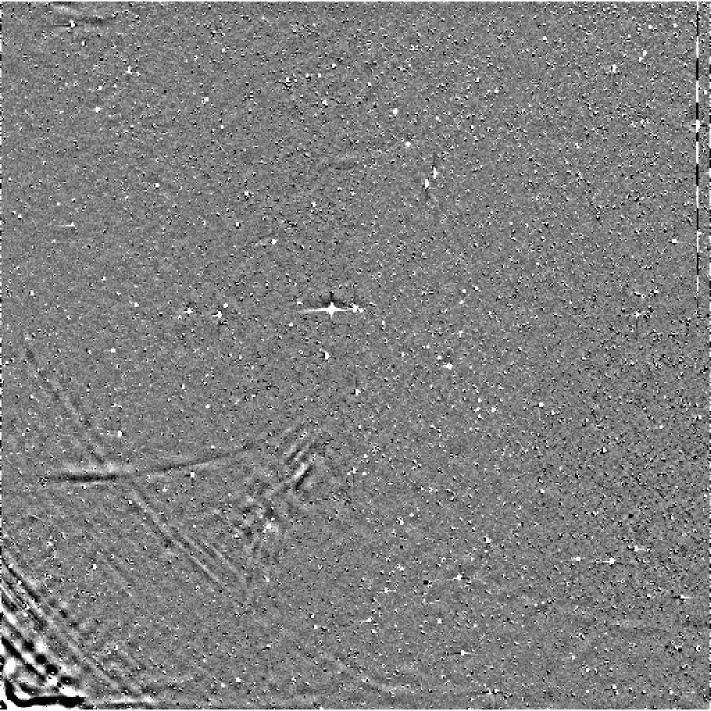
Figure 1: Panels showing the various stages of the image-level data processing using asteroid (2429) Schurer as an example, observed during Sector 2, by Camera #1, CCD #3. The left column shows the $10^{\prime}\times 10^{\prime}$ vicinity of the target, the middle column shows the neighbourhood ($3.7^{\circ}\times 1.4^{\circ}$) area while the right column is the full CCD frame, all at the TESS FFI cadence 2018247095941 (JD 2458365.92767). Images in the first row show the original unprocessed data. The second row is the difference in the background structure with respect to a frame where the Earth and Moon were below the sun-shade of TESS. The large-scale variations due to the stray light are clearly visible. The third row shows the difference between the first two rows. The fourth row shows the naive difference between the target image and the median differential-background reference image. The residuals due to the uncorrected differential velocity aberration are clearly visible. The fifth row shows the results of the image convolution followed by subtraction. This step also makes the TESS-specific, but otherwise comparatively faint vertical CCD stripes visible. In addition, the left stamp in this row shows that the sources, even ones brighter than the target objects are completely removed, with some residual structure only visible at a much brighter star at the upper-right corner of this stamp. Images in the sixth row show the results of the stripe removal process. The target at the center is clearly visible.

3 Data reduction and photometry

As it was mentioned above, the whole data processing of this catalogue was based on the observations performed by Camera #1 while surveying TESS sectors ranging from 1 up to 13. The processing has been carried out on a per-CCD basis, executing the same set of routines on the $13\times 4=52$ blocks of images corresponding to a single-sector-single-CCD acquisition run. The pipeline providing the light curves is exclusively based on the FITSH package (Pál, 2012). In this section we summarize the main steps of the photometric processing.

3.1 CCD-level steps

Each of the CCD image series is processed as follows. Based on the available orbital and pointing data, we selected nearly a dozen of frames called individual median reference frames (IMRFs) spanning a $\sim 2$-day period long interval close to the center of the observations evenly. These frames coincide for all of the four CCDs for a given sector, i.e., these correspond to the same cadence and usually have a time step of 4 hours between each frame. Another set of criteria was based on the constraint that both the Sun and the Moon should have been below the sun-shade of the spacecraft, meaning that both the Sun-TESS-boresight and the Moon-TESS-boresight angle should have been larger than $90^{\circ}$. This combined selection criteria ensured the lack of stray light in all of the cameras at the same time while the duration ensured an expected coverage of several tens of pixels of a main-belt asteroid while still keeping the differential velocity aberration at a considerably low level. In addition to the aforementioned selection criteria, if a prospective frame was flagged with a “reaction wheel desaturation event” (see Tenenbaum & Jenkins, 2018), the next or previous frame was selected instead.

In the next step, IMRFs were used to create a median image, employed as a median differential background reference image (MDBRI). This MDBRI was then subtracted from all of the images acquired by the same CCD in the same sector and the resulting differences were smoothed using a median window filtering combined with spline interpolation with a grid size of $64\times 64$ pixels. This step allowed the derivation of large-scale background variations and nicely helped to minimize and model the variations inducted by scattered light and zodiacal light. The derived background variations were then subtracted from all of the images and image convolution were applied between the MDBRI and these background-subtracted images. Note that this step does not subtract the intrinsic background since such a background practically does not exist for TESS images due to the very strong confusion and large pixel size. The image convolution steps correct not only for the PSF variations but for the offsets inducted by the differential velocity aberration as well. The latter one can be as large as one tenth of a pixel throughout a sector and it is the most prominent further away from the spacecraft boresight (which includes Camera #1 CCDs #3 and #4, which are the closest to the ecliptic plane). Once the convolved MDBRIs are derived, the resulting residual image was processed by a spline-smoothed median window filtering with a block size of $1\times 64$ pixels. This filtering removed the vertical stripes exposed in the TESS CCDs in parallel with the increased stray light. The steps of the aforementioned processing are displayed in Fig. 1 via the example of (2429) Schurer.

Figure 2: Folded light curve of (692) Hippodamia, having a rotation period $P=8.9993\,{\rm h}$. While this rotation period satisfies the Nyquist criterion, the phase coverage is not uniform due to the $P/C$ ratio of $\sim 18$.

Figure 3: Object light curve plots for (354) Eleonora (left column of 3 individualplots) and (220281) 2003 BA₄₇ (right column of 3 individual plots). These plots are available for all of the 9912 objects presented in this study.

3.2 Target astrometry and photometry

These cleared images were then used as the input of the aperture photometry where the centroids are computed by the EPHEMD tool with TESS set as the observer’s location. Absolute astrometric plate solutions have been derived using the Gaia DR2 catalogue (Gaia Collaboration et al., 2016, 2018) while the projection function was obtained by a third-order Brown-Conrady model on the top of tangential projection with additional refinements using a third-order polynomial expansion. The fluxes are extracted using the proper way needed to interpret convolved differential images (see Eq. 83 in Pál, 2009). The zero-point of the light curves were obtained using a global fit against the GAIA DR2 RP magnitudes. Due to the almost perfect overlap of the TESS and GAIA RP passbands – see also Fig. 1 in Ricker et al. (2015) and Fig. 3 in Jordi et al. (2010) – this yields a good and accurate match of the zero point. However, offsets can be presented due to the PSF variations across the field-of-view of the fast TESS optics. We note here that the formal uncertainties does not include the respective uncertainty of this offset. Individual light curve files were then generated by transposing the photometric results and flagged afterwards according to the quality flags presented in the TESS FFI headers (Tenenbaum & Jenkins, 2018). Light curves with insufficient number of data points were removed from the database and the post-filtering of these remaining light curves also added additional types of quality flags (see Table 1). This post-filtering process includes exclusion of the points with high formal photometric uncertainty, outlier detection based on histogram clipping and manual removal of points in the most prominent cases.

The filtered light curves were then analyzed by performing a period search. This period search was based on fitting a sinusoidal variation in parallel with the decorrelation of the phase angle variations up to the second order (see also Sec. 4.2 later on). The most dominant frequency was computed by interpolating in the vicinity of the frequency spectrum were the root mean square of the aforementioned fit residual was found to be the smallest (see Section 4.2). The light curves were then folded and binned after phase angle correction. Folding was performed with two periods, one corresponding to the dominant frequency while the other period we used was twice the dominant period, assuming a double-peaked light-curve generated by the rotation of an elongated body.

In total, 9912 objects are included in the present data release, for which accurate light curve information were derived with a reasonable significance. Out of these 9912 objects, 125 have only provisional designations and therefore are not numbered minor planets.

3.3 Sampling characteristics

The observing strategy of TESS is highly deterministic compared to many of the surveys and ground-based observations. Namely, the cadence is strictly $C=0.5\,{\rm h}$ for a nearly uninterrupted observing period of $L\lesssim 25-28\,{\rm d}$. This property implies the Nyquist criterion which does not allow the unambiguous rotation characterization for objects having a period of $P\leq 2C=1\,{\rm h}$. This is interesting for small objects, having a size of approximately or smaller than the spin barrier limit of $\sim 100\,{\rm m}$: such objects can rotate faster than $\sim 2.2\,{\rm h}$ (Pravec & Harris, 2000).

The strict cadence also yields sampling artefacts of objects having a rotation period which is close to the integer multiple of the cadence $C$. For instance, (692) Hippodamia has a rotation period of $P=8.9993\,{\rm hours}$, which is almost exactly $18$ times longer than the TESS FFI cadence (see Fig. 2). In order to characterize the strength of this sampling effect, let us assume that the period of the object is $P=nC+\varepsilon$ where $\varepsilon$ represent a short time difference and $n$ is an integer number (e.g. $n=18$ and $\varepsilon=-0.0007\,{\rm h}$ for (692) Hippodamia). In order to fully sample the rotational phase domain, one should expect that the second instance ($t=C$) has the same phase as the last phase after at or around the $k$th rotation where for the total observation timespan is $L\approx kP$. Here $k$ is also an integer, the total number of rotations covered during the observations. The phases are equal if $(knC/P)-(C/P)=k$, from which we can compute that $CP/L$ should be smaller than $|\varepsilon|$. This limit for (692) Hippodamia is $|\varepsilon|_{692}=(1/2\,{\rm h})\cdot(8.9993\,{\rm h})/(25\,{\rm d})\approx 0.0075\,{\rm h}$, definitely larger than $|\varepsilon|=0.0007\,{\rm h}$, we obtained above for this object, resulting in a stroboscopic effect. This stroboscopic effect is also present in K2 observations, see e.g. the case of (14791) Atreus in Szabó et al. (2017).

4 Database products and structures

Per-object data products were saved and stored in accordance with the aforementioned steps. The primary data products include four files per object, namely:

• the light curve file, containing the time series of the brightness measurements for a particular object;

• the residual r.m.s. frequency spectrum;

• a metadata file (best-fit rotation frequency, peak-to-peak amplitude, light curve type); and

• validation sheets, including the plots of the aforementioned data products,

• and per-object summary plots and slides, including the folded light curve with the most likely rotation period.

In the following, we describe these data products in more detail. The full data release is going to be available from the web address of http://archive.konkoly.hu/pub/tssys/dr1/.

4.1 Light curve files

The light curve files basically represent the post-transposition stage of the photometric output. Since photometry is performed on a per-frame basis and a single call to the photometric task (FITSH/fiphot) performs the flux extraction for all of the minor planets associated with that particular frame, light curve files also include the target name, the timestamp, the $(x,y)$ pixel coordinates and estimations for the background structure. Although differential imaging analysis and the subsequent photometry yields zero local background on subtracted images in theory, some artefacts – such as stray light spikes, unmasked blooming, prominent residual structures around bright but unsaturated stars – cause deviations from the zero level. Such information is therefore useful for further filtering of outliers and associate quality flags to the photometric data points. In addition to the aforementioned data, light curve files are extended with three additional columns showing the phase angle values, observer-centric distances and heliocentric distances.

4.2 Residual spectra

Residual spectra are generated by frequency scanning with a step size and coverage in accordance with the TESS sector time-span and the TESS FFI cadence, respectively. Namely, the total time-span of $\sim 27$ days on average imply a stepsize of $\Delta f=0.01\,{\rm c/d}$ while the Nyquist criterion maximizes the scanning interval in $f_{\rm max}=24\,{\rm c/d}$. The residual spectrum is then computed for a certain input frequency $f$ by minimizing the parameters $A$, $B$, and $k_{i}$ ($i=0,1,2$) for the model function

$$m(t) = \sum\limits_{i=0}^{2}k_{i}[\alpha(t)-\alpha_{0}]^{i}+$$

$$+A\cos[2\pi f(t-T_{0})]+B\sin[2\pi f(t-T_{0})].$$

where $m(t)$ is the observed magnitude (corrected for the variations in the solar and observer distances) at the instance $t$, $\alpha$ is the phase angle, $\alpha_{0}$ is the mean phase angle throughout the observations, and $T_{0}$ is an approximate mid-time of the observations. The actual values of $\alpha_{0}$ and $T_{0}$ do not alter the residuals (hence the spectra), however, setting the aforementioned values helps to minimize the numerical round-off errors and $k_{0}$ can also be interpreted as a mean brightness magnitude throughout the observations.

4.3 Metadata

In the case of the light curve and residual spectrum analysis, metadata represents the rotation frequency (and/or equivalently, the rotation period), the characteristics of the light curve shape and the peak-to-peak amplitude as well as any associated external database. While the processing scripts store metadata in separate files in a form of key-value pairs, the final data product includes a list of concatenated metadata in a tabular form.

In addition, this metadata table is extended with various large asteroid database information for convenience and further analysis. This information can be used to create additional types of statistics and have estimations for biases (see Sec. 5 for examples). In our published database, we included the most recent version of the synthetic proper orbital elements of Knežević & Milani (2000), as available online, the asteroid family catalog Version 3 of Nesvorný, Brož & Carruba (2015) and the most recent version of the Asteroid Lightcurve Database (LCDB, Warner, Harris & Pravec, 2009). Of course, the overlap with neither of the aforementioned databases are complete and there are only 1563 objects for which both proper orbital elements and LCDB data are available.

4.4 Validation plots

For a quick manual vetting of the results of the photometric analysis, we create a four-panel summary plot for each object. The four plots are the unfolded light curve, the residual spectrum, the folded light curve with the dominant period and the folded light curve with the double of the dominant period.

4.5 Object light curve plots and slides

These plots contain the same information as the validation plots, but in a bit different arrangement and these display only a single folded light curve with the most likely rotation period. The plots also show this rotation period in the units of hours. We note here that the time instances for both the plots and all of the light curve data products are given in in Julian Days (JDs). As an example, two of such object light curve plots are displayed in Fig. 3 for the objects (354) Eleonora and (220281) 2003 BA₄₇. These objects represent the bright end and the faint end of our catalogue.

5 Comparison with existing databases

5.1 Asteroid Lightcurve Database – LCDB

The most comprehensive database available in the literature is the Asteroid Lightcurve Database (LCDB, see Warner, Harris & Pravec, 2009). The most recent (August 2019) release of this database contains $4842$ objects for which a valid rotation period and brightness variation amplitude is associated. While this amount of data is nearly half of the entries available in the TESS minor planet data, the LCDB cites $2788$ bibliographic sources (concerning the entire database), therefore one should consider the inhomogeneity while interpreting LCDB statistics. However, we expect that the aforementioned quality constraints of selecting $4842$ objects ensure the robustness of the data products.

Figure 4: The left panel shows the rotation periods of the 624 objects for which reliable rotation characteristics (i.e. periods and amplitudes) are available both in the LCDB catalogue and the TESS observations presented in this paper. The thick line and the two dashed lines correspond to the same rotation frequencies as well as the $1:2$ and $2:1$ ratios, respectively. The right panel displays the histogram of the frequency ratios of the objects available both in the LCDB catalogue and the presented TESS minor planet catalog. In total, $\sim 80\%$ of the matched objects have the same derived rotation periods while in the case of $\sim 8\%$ of the objects, the newly derived preferred periods are either the double or half of the periods available in the LCDB. TESS measurements clearly identified longer rotation periods for the majority of the remaining $\sim 60$ objects.

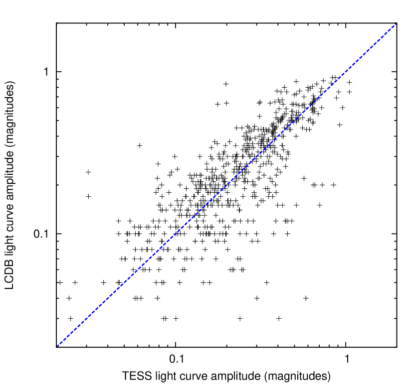
Figure 5: Left panel: light curve peak-to-peak amplitudes for the 624 objects where rotation characteristics are available both in the LCDB catalogue and the TESS observations presented here. Right panel: the histogram of the distribution of the amplitude ratios. The thick vertical line shows the unity ratio while the thin vertical dashed line at $\sim 1.076$ shows the median value of the amplitude ratios.

In total, we identified $624$ objects which are available both in TSSYS-DR1 and LCDB (with sufficiently strong qualification). We note here that there are $1535$ objects available both in TSSYS-DR1 and LCDB if we do not consider the amplitude quality criteria mentioned above. In Figs. 4 and 5 we displayed the rotation frequency and amplitude correlations, respectively, between the two databases. Considering the rotation periods, we found that the agreement is perfect for $\sim 80\%$ of the objects while there are a few dozens of objects where the double-peaked ambiguity yields a $1:2$ or $2:1$ ratio. The amount of such ambiguities is roughly the the same (19 vs. 28) for the two ratios. Otherwise, it is worth to mention here that TESS clearly identifies the objects with longer periods better, suspecting an unclear origin of the otherwise shorter reported periodicity in LCDB (see the points above the $1:1$ and $2:1$ line on the left panel of Fig. 4 or the histogram distribution at the right tail on the right panel of the same Figure).

Regarding to the interpretation of the correlations between amplitudes (see Fig. 5), the larger amplitudes present in the LCDB is a clear signature of the bias in the TESS observations. Namely, TESS observes minor planets close to the opposition, i.e. at small phase angles while LCDB contains many kinds of observations (yielding better coverage in phase angles), not just ones close to the opposition. According to the expectations (Zappala et al., 1990), higher phase angles would yield higher amplitudes, which can explain the shift in the correlation diagram and the corresponding histogram. However, one should note that because of this TESS-specific observing constraint as well as due to the fact that the presented data release contains only a single epoch while LCDB aggregates data from many observing runs, such a statistical comparison between TESS and LCDB amplitudes needs to be considered tentative. While the presented TESS data series are highly homogeneous, it shows an amplitude characteristics only for a single observing geometry, leaving many aspects of shape characteristics ambiguous.

Figure 6: The 6 minor planets for which both Kepler/K2 and TESS measurements are available. 3 out of these 6 objects are Jupiter Trojans while the another two are main-belt asteroids. With the exception of the Trojan asteroid (65210) Stichius, the periods match within $1.5\%$. The agreement for (24534) 2001 CX₂₇ and (42573) 1997 AN₁ are less than one tenth of a percent. (65210) Stichius show a difference of $\sim 8\%$ between the derived periods.

5.2 K2 Solar System Studies – K2SSS

While having scanned various fields close to the ecliptic plane, the K2 mission (Howell et al., 2014) also provided a highly efficient way to provide uninterrupted observations for various classes of Solar System objects. These classes include not only main-belt and Trojan asteroids but trans-Neptunian objects (Pál et al., 2015), irregular satellites of giant planets (Kiss et al., 2016; Farkas-Tak cs et al., 2017), and the Pluto-Charon system (Benecchi et al., 2018). K2 observations also implied the discovery of the satellite of (225088) 2007 OR₁₀ (Kiss et al., 2017) when its slow rotation was detected (Pál et al., 2016).

With the exception of the discovery and photometry of the trans-Neptunian object (506121) 2016 BP₈₁ (Barensten et al., 2017), all of these object classes were measured as targeted observations, i.e. with pre-allocated K2 target pixel files (arranged into special boomerang-shaped pixel blocks). In the case of main-belt and Trojan asteroids, there are examples of targeted observations (Marciniak et al., 2019; Szabó et al., 2017; Ryan, Sharkey & Woodward, 2017) as well as photometry on contiguous superstamps (Szabó et al., 2016; Molnár et al., 2018) when asteroids serendipitously crossed these celestial areas. However, the data reduction pattern does not differ significantly for pre-allocated reductions and the analysis of contiguous superstamps with the exception of the aforementioned querying of the objects (by tools like EPHEMD) in the latter case. See, e.g., Szabó et al. (2017) for a detailed description about the data reduction for K2 minor planet observations observations.

In order to compare the objects observed by any initiative of the K2 Solar System Surveys with this recent TESS-based photometry, we identifies 6 main-belt and Trojan objects that were observed both by K2 and TESS. These were (24534) 2001 CX₂₇, (24537) 2001 CB₃₅, (37750) 1997 BZ, (42573) 1997 AN₁, (45086) 1999 XE₄₆ and (65210) Stichius. We found that the derived rotation periods match perfectly in $5$ of the $6$ cases, see Fig. 6. There was only a slight offset for (65210) Stichius, due to its faintness and long rotation period of $\sim 32$  hours.

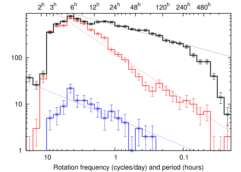
Figure 7: The number of objects as the function of their periods, provided by various databases. The black curve shows the period distribution for TSSYS-DR1 ($9912$ objects), the red curve shows the period distribution for the $4842$ LCDB objects for which a valid rotation period and brightness variation amplitude have been derived at the same time. The blue curve shows the period distribution for $113$ serendipitous main-belt asteroids provided by the analysis of three K2 superstamps. The thin dashed lines guide the eye to provide a tentative slope at the long period (low frequency) parts of these distributions.

5.3 Period statistics

In Fig. 7 we displayed the histograms of the detected rotation periods for this TESS-based asteroid survey, the LCDB and the K2 serendipitous main-belt asteroid detections on the M35 and Neptune-Nereid fields (Szabó et al., 2016), as well as on the Uranus field (Molnár et al., 2018). A tentative fit in the long-period part of these histograms clearly show that both ground-based and shorter duration but otherwise uninterrupted space-borne measurements underestimate the number of objects in the population of slow rotators. Therefore, we can safely conclude that the nearly one-month long continuous data acquisition of TESS would provide us the most unbiased coverage and confirmation of slowly rotating asteroids. However, it is still an interesting question where the cut-off of TESS is, above which the rotation period statistics become significantly biased. The divergence between the LCDB and TESS histograms stars at rotation periods of $8-10$ hours. Below this period, the two statistics nicely agree down to the periods of $\sim 2$ hours range.

6 Summary

In this paper we presented the first data release of the complete Southern Survey of the Transiting Exoplanet Survey Satellite in terms of analysis of bright, main-belt and Trojan asteroids crossing the field-of-view of Camera #1. This survey triples the number of asteroids with accurately determined rotation characteristics. Another advantage of the presented catalogue is that it is fully homogeneous considering both data acquisition and data processing principles. Further fine-tuning in the pipeline presented here is also possible, and we have the intention to process and add further object classes, including Centaurs, trans-Neptunian objects and near-Earth objects (see also Milam et al., 2019).

TESS is now observing the Northern Hemisphere, opening the possibilities to re-observe many of the objects presented in this data release with a completely different observing geometry with respect to the spin-axis orientation of these bodies. Such further observations would help us to interpret the derived light curve characteristics, specifically the amplitude in a more accurate manner and therefore helping the analysis for a more accurate comparison with LCDB. We should also express our hope that the extended mission of TESS would include wide coverage of the ecliptic plane, further expanding our collection of asteroid observations and increase the number of multi-epoch observations.

References

- Barensten et al. (2017) Barentsen, G.; Pál, A.; Sárneczky K., & Molnár, L. 2017, MPC 102428
- Benecchi et al. (2018) Benecchi, S. D.; Lisse, C. M.; Ryan, E. L.; Binzel, R. P.; Schwamb, M. E.; Young, L. A. & Verbiscer, A. J. 2018, Icarus, 314, 265
- Borucki et al. (2010) Borucki, W. J., Koch, D., Basri, G., et al. 2010, Science, 327, 977
- Delbo et al. (2015) Delbo, M., Mueller, M., Emery, J. P., Rozitis, B., Capria, M. T., 2015, Asteroid Thermophyiscal Modeling, in: Asteroids IV, eds. P. Michel, F.E. DeMeo & W.F. Bottke, University of Arizona Press, Tucson
- Farkas-Tak cs et al. (2017) Farkas-Takács, A.; Kiss, Cs.; Pál, A.; Molnár, L.; Szabó, Gy. M.; Hanyecz, O.; Sárneczky, K.; Szabó, R.; Marton, G.; Mommert, M.; Szakáts, R.; Müller, T. & Kiss, L. L. 2017, AJ, 154, 119
- Gaia Collaboration et al. (2016) Gaia Collaboration: T. Prusti et al., 2016, A&A, 595, A1
- Gaia Collaboration et al. (2018) Gaia Collaboration; Brown, A. G. A.; Vallenari, A.; Prusti, T.; de Bruijne, J. H. J.; Babusiaux, C.; Bailer-Jones, C. A. L., 2018, A&A, 616, A1
- Howell et al. (2014) Howell, S. B., Sobeck, C., Haas, M., et al. 2014, PASP, 126, 398
- Jordi et al. (2010) Jordi, C.; Gebran, M.; Carrasco, J. M.; de Bruijne, J.; Voss, H.; Fabricius, C.; Knude, J.; Vallenari, A.; Kohley, R.; Mora, A, 2010, A&A, 523, A48
- Kiss et al. (2016) Kiss, Cs.; Pál, A.; Farkas-Takács, A. I.; Szabó, Gy. M.; Szabó, R.; Kiss, L. L.; Molnár, L.; Sárneczky, K.; Müller, T. G.; Mommert, M.; Stansberry, J. 2016, MNRAS, 457, 2908
- Kiss et al. (2017) Kiss, Cs.; Marton, G.; Farkas-Takács, A.; Stansberry, J.; Müller, Th.; Vinkó, J.; Balog, Z.; Ortiz, J.-L. & Pál, A. 2017, ApJL, 838, 1
- Kiss et al. (2019) Kiss, Cs.; Szakáts, R.; Marton, G.;Farkas-Takács, A.; Müller, Th.; & .; Alí-Lagoa, V. 2019, Small Bodies: Near and Far database of thermal infrared measurements of small Solar System bodies Release Note: Public Release 1.2, 2019 March 29
- Knežević & Milani (2000) Knežević, Z. & Milani, A. 2000, CeMDA, 78, 17
- Marciniak et al. (2019) Marciniak, A.; Alí-Lagoa, V.; Müller, T. G.; Szakáts, R.; Molnár, L.; Pál, A.; Podlewska-Gaca, E.; Parley, N. et al. 2019, A&A, 625, A139
- Milam et al. (2019) Milam, S. N.; Hammel, H. B.; Bauer, J.; Brozovic, M.; Grav, T.; Holler, B. J.; Lisse, C.; Mainzer, A.; Reddy, V.; Schwamb, M. E.; Spahr, T.; Thomas, C. A.; Woods, D 2019, Combined Emerging Capabilities for Near-Earth Objects (NEOs), White Paper for NASA on astrophysics assets, e-print (arXiv:1907.08972)
- Molnár et al. (2018) Molnár, L.; Pál, A.; Sárneczky, K.; Szabó, R.; Vinkó, J.; Szabó, Gy. M.; Kiss, Cs.; Hanyecz, O.; Marton, G.; Kiss, L. L. 2018, ApJS, 234, 37
- Müller et al. (2009) Müller, T. G., Lellouch, E, Böhnhardt, H. et al. 2009, EM&P, 105, 209
- Nesvorný, Brož & Carruba (2015) Nesvorný, D.; Brož, M. & Carruba, V. 2015, in Asteroids IV, Patrick Michel, Francesca E. DeMeo, and William F. Bottke (eds.), University of Arizona Press, Tucson, 895 pp.
- Pál (2009) Pál, A. 2009, PhD thesis (arXiv:0906.3486)
- Pál (2012) Pál, A. 2012, MNRAS, 421, 1825
- Pál et al. (2015) Pál, A.; Szabó, R.; Szabó, Gy. M.; Kiss, L. L.; Molnár, L.; Sárneczky, K. & Kiss, Cs. 2015, ApJL, 804, 45
- Pál et al. (2016) Pál, A.; Kiss, Cs.; Müller, Th. G.; Molnár, L.; Szabó, R.; Szabó, Gy. M.; Sárneczky, K. & Kiss, L. L. 2016, AJ, 151, 117
- Pál, Molnár & Kiss (2018) Pál, A., Molnár, L. & Kiss, Cs. 2018, PASP, 130, 114503
- Pravec & Harris (2000) Pravec, P. & Harris, A. W. 2000, Icarus, 148, 12
- Ricker et al. (2015) Ricker, G. R. et al. 2015, J. Astron. Telesc. Instrum. Syst. Vol. 1, id. 014003
- Ryan, Sharkey & Woodward (2017) Ryan, E. L.; Sharkey, B. N. L. & Woodward, Ch. E. 2017, AJ, 153, 116
- Szabó et al. (2015) Szabó, R., Sárneczky, K., Szabó, Gy. M., et al. 2015, AJ, 149, 112
- Szabó et al. (2016) Szabó, R.; Pál, A.; Sárneczky, K.; Szabó, Gy. M.; Molnár, L.; Kiss, L. L.; Hanyecz, O.; Plachy, E. & Kiss, Cs. 2016, A&A, 596, A40
- Szabó et al. (2017) Szabó, Gy. M.; Pál, A.; Kiss, Cs.; Kiss, L. L.; Molnár, L.; Hanyecz, O.; Plachy, E.; Sárneczky, K.; Szabó, R. 2017, A&A, 599, A44
- Szakáts et al. (2017) Szakáts, R.; Kiss, Cs.; Marton, G.; Varga-Verebélyi, E.; Müller, T. & Pál, A. 2017, European Planetary Science Congress, id. EPSC2017-223
- Tenenbaum & Jenkins (2018) Tenenbaum, P. & Jenkins, J. M., 2018: TESS Science Data Products Description Document, EXP-TESS-ARC-ICD-0014 Rev D.
- Warner, Harris & Pravec (2009) Warner, B. D., Harris, A. W. & Pravec, P. Updated 2019 August 14, 2009, Icarus, 202, 134
- Zappala et al. (1990) Zappala, V.; Cellino, A.; Barucci, A. M.; Fulchignoni, M.; Lupishko, D. F. 1990, A&A, 231, 548