A Support Detection and Root Finding Approach for Learning High-dimensional Generalized Linear Models

Abstract

Feature selection is important for modeling high-dimensional data, where the number of variables can be much larger than the sample size. In this paper, we develop a support detection and root finding procedure to learn the high dimensional sparse generalized linear models and denote this method by GSDAR. Based on the KKT condition for $\ell_{0}$-penalized maximum likelihood estimations, GSDAR generates a sequence of estimators iteratively. Under some restricted invertibility conditions on the maximum likelihood function and sparsity assumption on the target coefficients, the errors of the proposed estimate decays exponentially to the optimal order. Moreover, the oracle estimator can be recovered if the target signal is stronger than the detectable level. We conduct simulations and real data analysis to illustrate the advantages of our proposed method over several existing methods, including Lasso and MCP.
Keywords: High-dimensional generalized linear models, Sparse Learning, $\ell_{0}$-penalty, Support detection, Estimation error.
Running title: GSDAR

1 Introduction

In generalized linear models (GLMs) [21, 19], the response variable $Y$ follows an exponential family distribution with density $f(y;\theta)=\exp[y\theta-c(\theta)+d(y)]$, where $c(\cdot)$ and $d(\cdot)$ are known functions, $\theta=\mbox{\bf x}^{T}\bm{\beta}^{*}$, x and $\bm{\beta}^{*}$ represent the $p$-dimension vectors of predictors and the target regression coefficients, respectively. Let $E(y_{i})=\mu_{i}$, where $\mu_{i}$ is some function of $\theta_{i}=\mbox{\bf x}_{i}^{T}\bm{\beta}$.

When the number of predictors $p$ exceeds the number of sample size $n$, it is often reasonable to assume that the model is sparse in the sense that there are only small portion of significant predictors. In this case, one may estimate $\bm{\beta}^{*}$ by the following $\ell_{0}$ minimization problem

$$\begin{split}&\underset{\bm{\beta}\in\mathbb{R}^{p}}{\mbox{min}}~{}\mathcal{L}(\bm{\beta})\\ &\mbox{subject~{}to}~{}~{}\|\bm{\beta}\|_{0}\leq s,\end{split}$$ (1)

where $\mathcal{L}(\bm{\beta})=-\frac{1}{n}\sum_{i=1}^{n}\big{[}y_{i}\mbox{\bf x}_{i}^{T}\bm{\beta}-c(\mbox{\bf x}_{i}^{T}\bm{\beta})+d(y_{i})\big{]}$ is the negative log likelihood function, $\|\bm{\beta}\|_{0}$ is defined as the number of nonzero elements of $\bm{\beta}$, and $s>0$ is a tuning parameter that controls the sparsity level. Due to the computational difficulty of solving (1), many researchers have proposed other penalized methods for variable selection and estimation in high-dimensional GLMs. [23, 29] extended the Lasso method [28] from linear regression to GLMs. [20] proposed the group lasso for logistic regression. [6] developed coordinate descent to solve the elastic net [37] penalized GLMs. Path following proximal gradient descent [22] was adopted in [32, 14] to solve the SCAD [4] and MCP [35] regularized GLMs. In [12], the authors propose a DC proximal Newton (DCPN) method to solve GLMs with nonconvex sparse promoting penalties such as MCP/SCAD. Recently, [31, 34, 26] considered Newton type algorithm for solving sparse GLMs.

In this paper, we propose an approach to variable selection and estimation in high-dimensional GLMs named GSDAR by a nontrivial extension of the support detection and rooting finding (SDAR) algorithm [10] which is proposed to solve linear regression models and can not be applied to analyze binary data, categorical variables in GLMs. GSDAR is a computational algorithm motivated from the KKT conditions for the Lagrangian version of (1). It generates a sequence of solutions $\{\bm{\beta}^{k}\}_{k}$ iteratively, based on support detection using primal and dual information and root finding. Under some certain conditions on $\mathcal{L}$ and sparsity assumptions on the regression coefficient $\bm{\beta}^{*}$, we prove that the estimation errors decay exponentially to the optimal order. Moreover, the oracle estimator can be recovered with high probability if the target signal is over the detectable level.

The rest of this paper is organized as follows. In Section 2, we present the detail derivation of GSDAR algorithm. In Section 3, we bound the estimation error of GSDAR. In Section 4, we extend GSDAR algorithm to AGSDAR, an adaptive version of GSDAR. In Section 5, we demonstrate GSDAR and AGSDAR on the simulation and real data via comparing with state-of-the-art methods. We conclude in Section 6. Proofs for all the lemmas and theorems are provided in the Appendix.

2 Derivation of GSDAR

First, we introduce some notations used throughout the paper. We write $n\gtrsim\log(p)$ to mean that $n\geq c\log(p)$ for some universal constant $c\in(0,\infty)$. Let $\|\bm{\beta}\|_{q}=(\sum_{i=1}^{p}|\beta_{i}|^{q})^{\frac{1}{q}}$ denote the $q$ ($q\in[1,\infty]$) norm of a vector $\bm{\beta}=(\beta_{1},...,\beta_{p})^{T}\in\mathbb{R}^{p}$. Let supp$(\bm{\beta})$=$\{i:\beta_{i}\neq 0,~{}i=1,...,p\}$ denote the support of $\bm{\beta}$, and $A^{*}=\mathrm{supp}(\bm{\beta}^{*}).$ Let $|A|$ denote the length of the set $A$ and denote $\bm{\beta}_{A}=(\beta_{i},i\in A)\in\mathbb{R}^{|A|}$, $\bm{\beta}|_{A}\in\mathbb{R}^{p}$ with its $i\text{-}$th element $({\bm{\beta}|_{A}})_{i}=\beta_{i}1(i\in A)$, where $\textbf{1}(\cdot)$ is the indicator function. Denote ${\bf X}_{A}=(\mbox{\bf x}_{j},j\in A)\in\mathbb{R}^{n\times|A|}$, where $\mbox{\bf x}_{j}$ is $j$-th column of the covariate matrix ${\bf X}\in\mathbb{R}^{n\times p}$. $\|\bm{\beta}\|_{T,\infty}$ and $\|\bm{\beta}\|_{\min}$ denote the $T$-th largest elements (in absolute value) and the minimum absolute value of $\bm{\beta}$, respectively. $\nabla\mathcal{L}$ and $\nabla^{2}\mathcal{L}$ denote the gradient and Hessian of function $\mathcal{L}$, respectively.

The Lagrangian form of (1) is

$$\underset{\bm{\beta}\in\mathbb{R}^{p}}{\mbox{min}}~{}\mathcal{L}(\bm{\beta})+\lambda\|\bm{\beta}\|_{0}.$$ (2)

By similar arguments as Lemma 1 of [10], we obtain the following KKT condition of (2).

Lemma 2.1.

If $\bm{\beta}^{\diamond}$ is a minimizer of (2), then $\bm{\beta}^{\diamond}$ satisfies:

$$\left\{\begin{aligned} &\mbox{\bf d}^{\diamond}=-\nabla\mathcal{L}(\bm{\beta}^{\diamond}),\\ &\bm{\beta}^{\diamond}=H_{\lambda}(\bm{\beta}^{\diamond}+\mbox{\bf d}^{\diamond}),\end{aligned}\right.$$ (3)

where the $i$-th element of $H_{\lambda}(\cdot)$ is defined by

$$(H_{\lambda}(\bm{\beta}))_{i}=\left\{\begin{aligned} &0,&&&|\beta_{i}|\leq\sqrt{2\lambda},\\ &\beta_{i},&&&|\beta_{i}|\geq\sqrt{2\lambda}.\\ \end{aligned}\right.$$

Conversely, if $\bm{\beta}^{\diamond}$ and $\mbox{\bf d}^{\diamond}$ satisfy (3), then $\bm{\beta}^{\diamond}$ is a local minimizer of (2).

Proof.

See Appendix A. ∎

Let $A^{\diamond}=\text{supp}(\bm{\beta}^{\diamond})$, $I^{\diamond}=(A^{\diamond})^{c}$. From the definition of $H_{\lambda}(\cdot)$ and (3), we can conclude that

$$A^{\diamond}=\{i:|\beta^{\diamond}_{i}+d^{\diamond}_{i}|\geq\sqrt{2\lambda}\},\quad I^{\diamond}=\{i:|\beta^{\diamond}_{i}+d^{\diamond}_{i}|<\sqrt{2\lambda}\},$$

and

$$\left\{\begin{aligned} &\bm{\beta}_{I^{\diamond}}^{\diamond}=\textbf{0}\\ &\mbox{\bf d}_{A^{\diamond}}^{\diamond}=\textbf{0}\\ &\bm{\beta}_{A^{\diamond}}^{\diamond}\in\underset{\bm{\beta}_{A^{\diamond}}}{\mbox{argmin}}~{}\widetilde{\mathcal{L}}(\bm{\beta}_{A^{\diamond}})\\ &\mbox{\bf d}_{I^{\diamond}}^{\diamond}=[-\nabla\mathcal{L}(\bm{\beta}^{\diamond})]_{I^{\diamond}},\end{aligned}\right.$$

where

$$\widetilde{\mathcal{L}}(\bm{\beta}_{A^{\diamond}}) =\mathcal{L}(\bm{\beta}|_{A^{\diamond}})$$

$$=-\frac{1}{n}\sum_{i=1}^{n}\left[y_{i}\mbox{\bf x}_{i{(A^{\diamond})}}^{T}\bm{\beta}_{A^{\diamond}}-c\big{(}\mbox{\bf x}_{i{(A^{\diamond})}}^{T}\bm{\beta}_{A^{\diamond}}\big{)}+d(y_{i})\right].$$

If $\{\bm{\beta}^{k},\mbox{\bf d}^{k}\}$ can approximate $\{\bm{\beta}^{\diamond},\mbox{\bf d}^{\diamond}\}$ well, then $\{A^{k},I^{k}\}$ can also approximate $\{A^{\diamond},I^{\diamond}\}$ well, where $\{A^{k},I^{k}\}$ is expressed as

$$A^{k}=\{i:|\beta^{k}_{i}+d^{k}_{i}|\geq\sqrt{2\lambda}\},\quad I^{k}=\{i:|\beta^{k}_{i}+d^{k}_{i}|<\sqrt{2\lambda}\}.$$ (4)

Thus we get a new approximation pair $\{\bm{\beta}^{k+1}_{I^{k}},\mbox{\bf d}^{k+1}_{A^{k}},\bm{\beta}^{k+1}_{A^{k}},\mbox{\bf d}^{k+1}_{I^{k}}\}$ showed as follow:

$$\left\{\begin{aligned} &\bm{\beta}^{k+1}_{I^{k}}=\textbf{0}\\ &\mbox{\bf d}^{k+1}_{A^{k}}=\textbf{0}\\ &\bm{\beta}^{k+1}_{A^{k}}\in\underset{\bm{\beta}_{A^{k}}}{\mbox{argmin}}~{}\widetilde{\mathcal{L}}(\bm{\beta}_{A^{k}})\\ &\mbox{\bf d}^{k+1}_{I^{k}}=[-\nabla\mathcal{L}(\bm{\beta}^{k+1})]_{I^{k}},\\ \end{aligned}\right.$$ (5)

where

$$\widetilde{\mathcal{L}}(\bm{\beta}_{A^{k}}) =\mathcal{L}(\bm{\beta}|_{A^{k}})$$

$$=-\frac{1}{n}\sum_{i=1}^{n}\left[y_{i}\mbox{\bf x}_{i{(A^{k})}}^{T}\bm{\beta}_{A^{k}}-c\big{(}\mbox{\bf x}_{i{(A^{k})}}^{T}\bm{\beta}_{A^{k}}\big{)}+d(y_{i})\right]$$

If we have the prior information that $\parallel\bm{\beta}^{*}\parallel_{0}=K\leq T$, then we set

$$\sqrt{2\lambda}=\parallel\bm{\beta}^{k}+\mbox{\bf d}^{k}\parallel_{T,\infty}$$ (6)

in (4). Thus $|A^{k}|=T$ in every iteration due to this $\lambda$. Let $\bm{\beta}^{0}$ be an initial value, then we get a sequence of solutions $\{\bm{\beta}^{k},k\geq 1\}$ by using (4) and (5) with the $\lambda$ in (6).

The GSDAR algorithm is described in Algorithm 1.

Algorithm 1 GSDAR

1:  Input: $\bm{\beta}^{0}$, $T$, $\mbox{\bf d}^{0}=-\nabla\mathcal{L}(\bm{\beta}^{0})$; $k=0$

2:  for $k=0,1,\ldots,$ do

3:     $A^{k}=\big{\{}j:|\beta^{k}_{j}+d^{k}_{j}|\geq\|\bm{\beta}^{k}+\mbox{\bf d}^{k}\|_{T,\infty}\big{\}}$, $I^{k}=(A^{k})^{c}$.

4:     $\bm{\beta}^{k+1}_{I^{k}}=\textbf{0}$.

5:     $\mbox{\bf d}^{k+1}_{A^{k}}=\textbf{0}$.

6:     $\bm{\beta}^{k+1}_{A^{k}}=\underset{\bm{\beta}_{A^{k}}}{\mbox{argmin}}~{}\widetilde{\mathcal{L}}(\bm{\beta}_{A^{k}})$.

7:     $\mbox{\bf d}^{k+1}_{I^{k}}=[-\nabla\mathcal{L}(\bm{\beta}^{k+1})]_{I^{k}}$.

8:     if $A^{k}=A^{k+1}$, then

9:      Stop and denote the last iteration $\bm{\beta}_{\widehat{A}}$, $\bm{\beta}_{\widehat{I}}$, $\mbox{\bf d}_{\widehat{A}}$, $\mbox{\bf d}_{\widehat{I}}$.

10:     else

11:      $k=k+1$

12:     end if

13:  end for

14:  Output: $\widehat{\bm{\beta}}=(\bm{\beta}^{\mathrm{T}}_{\widehat{A}}$, $\bm{\beta}^{\mathrm{T}}_{\widehat{I}})^{\mathrm{T}}$ as the estimates of $\bm{\beta}^{*}$.

In Algorithm 1, we terminate GSDAR when $A^{k}=A^{k+1}$ for some $k$, because the sequences generated by GSDAR will not change. In Section 3, we will prove that under some regularity certain conditions on ${\bf X}$ and $\bm{\beta}^{*}$, with high probability $A^{*}=A^{k}=A^{k+1}$ in finite steps, i.e., the GSDAR will stop and whence the oracle estimator will be recovered.

3 Theoretical Properties

In this section, we will give the $\ell_{\infty}$ error bounds for the GSDAR estimator. Under some certain conditions, we show that $\|\bm{\beta}^{k}-\bm{\beta}^{*}\|_{\infty}$ achieves sharp estimation error. Furthermore, if the minimum value of target signal is detectable, GSDAR will get the oracle estimator in finite steps if $K$ is chosen just as the true model size $T$. We first introduce the following restricted invertibility conditions.

1. There exist constants $0<L<U\in(0,\infty)$ such that, for all different vectors $\bm{\beta}_{1}$ and $\bm{\beta}_{2}$ with $\|\bm{\beta}_{1}-\bm{\beta}_{2}\|_{0}\leq 2T$,

   $$0<L\leq\frac{(\bm{\beta}_{1}-\bm{\beta}_{2})^{T}\cdot\nabla^{2}\mathcal{L}(\widetilde{\bm{\beta}})\cdot(\bm{\beta}_{1}-\bm{\beta}_{2})}{\|\bm{\beta}_{1}-\bm{\beta}_{2}\|_{1}\|\bm{\beta}_{1}-\bm{\beta}_{2}\|_{\infty}}\leq U<\infty,$$

   where $\widetilde{\bm{\beta}}=\bm{\beta}_{1}+\nu(\bm{\beta}_{2}-\bm{\beta}_{1})$ for any $\nu\in(0,1)$.

2. $\|\bm{\beta}^{*}_{A^{*}}\|_{\min}\geq\frac{3c_{1}}{L}\sqrt{\frac{\log(p)}{n}}$, where $c_{1}$ is a universal numerical constant.

Remark 3.1.

Condition (C1) extends the the weak cone invertibility condition in [33]. This kind restricted strong convexity type regularity condition is needed in bounding the estimation error in high dimension statistics [36]. Condition (C2) is required to guarantee the target signal to be detectable in high dimension linear regressions.

3.1 $\ell_{\infty}$ error bounds

Theorem 3.1.

Assume (C1) holds with $0<U<\frac{1}{T}$. Set $K\leq T$ and $\bm{\beta}^{0}=\textbf{0}$ in Algorithm 1.

(i) Before Algorithm 1 terminates, we have

$$\|\bm{\beta}^{k}-\bm{\beta}^{*}\|_{\infty}$$

$$\leq\sqrt{(K+T)(1+\frac{U}{L})}(\sqrt{\xi})^{k}\|\bm{\beta}^{*}\|_{\infty}+\frac{2}{L}\|\nabla\mathcal{L}(\bm{\beta}^{*})\|_{\infty}.$$

where $\xi=1-\frac{2L(1-TU)}{T(1+K)}\in(0,1)$.

(ii) Assume the rows of ${\bf X}$ are i.i.d. sub-Gaussian with $n\gtrsim\log(p)$, then there exists universal constants $(c_{1},c_{2},c_{3})$ with $0<c_{i}<\infty$, $i=1,2,3$, such that with probability at least $1-c_{2}\exp(-c_{3}\log(p))$,

$$\|\bm{\beta}^{k}-\bm{\beta}^{*}\|_{\infty}$$

$$\leq\sqrt{(K+T)(1+\frac{U}{L})}(\sqrt{\xi})^{k}\|\bm{\beta}^{*}\|_{\infty}+\frac{2c_{1}}{L}\sqrt{\frac{\log(p)}{n}},$$

i.e.,

$$\|\bm{\beta}^{k}-\bm{\beta}^{*}\|_{\infty}\leq\mathcal{O}\left(\sqrt{\frac{\log(p)}{n}}\right)$$

with high probability if $k\geq\mathcal{O}\left(\log_{\frac{1}{\xi}}\frac{n}{\log(p)}\right).$

Proof.

See Appendix B. ∎

Remark 3.2.

The requirement $U<\frac{1}{T}$ is not essential since we can always rescale the loss function $\mathcal{L}$ to make it hold. This rescaling is equivalent to multiplying a step size to the dual variable in the the GSDAR algorithm. Let $\tau$ be this step size satisfying $0<\tau<\frac{1}{TU}$. Then, Theorem 3.1 still holds by replacing $\xi$ with $1-\frac{2\tau L(1-\tau TU)}{T(1+K)}\in(0,1)$.

Before we submit this work, We aware that [31] proposed the sparse Newton method to solve high dimensional logistic regression. The sparse Newton algorithm is similar to GSDAR with step size. However, [31] proved a fast local convergence result of $\bm{\beta}^{k}$ to the minimizer $\bm{\beta}^{\diamond}$ from the point view of optimization. Here, we bound the estimation error of $\bm{\beta}^{k}$ to the target $\bm{\beta}^{*}$ from the angle of statistics.

3.2 Support recovery

Theorem 3.2.

Assume (C1) and (C2) hold with $0<U<\frac{1}{T}$, and the rows of ${\bf X}$ are i.i.d. sub-Gaussian with $n\gtrsim\log(p)$. Set $K\leq T$ in Algorithm 1. Then with probability at least $1-c_{2}\exp(-c_{3}\log(p))$, $A^{*}\subseteq A^{k}$ if $k>\log_{\frac{1}{\xi}}9(T+K)(1+\frac{U}{L})r^{2}$, where $r=\frac{\|\bm{\beta}^{*}\|_{\infty}}{\|\bm{\beta}^{*}_{A^{*}}\|_{\min}}$ is the range of $\bm{\beta}^{*}$.

Proof.

See Appendix C. ∎

Remark 3.3.

Theorem 3.2 demonstrates that the estimated support via GSDAR can cover the true support with the cost at most $\mathcal{O}(\log(T))$ number of iteration if the minimum signal strength of $\bm{\beta}^{*}$ is above the detectable threshold $\mathcal{O}(\sqrt{\frac{\log(p)}{n}})$. Support recovery for sparse GLMs has also been studied in [12, 34, 26]. In [12], the authors propose a DC proximal Newton (DCPN) method to solve GLMs with nonconvex sparse promoting penalties such as MCP/SCAD. They derive an estimation error in $\ell_{2}$ norm with order $\mathcal{O}(\sqrt{\frac{K\log p}{n}})$ under similar assumptions as that of our (C1). And they show that the true support can be reconverted under the requirement $\|\bm{\beta}^{*}_{A^{*}}\|_{\min}\geq\mathcal{O}(\sqrt{\frac{K\log(p)}{n}}),$ which is stronger than our assumption (C2). The computational complexity of DCPN is worse than GSDAR since the DCPN is based on the multistage convex relaxation scheme to transform the original nonconvex optimizations into sequences of LASSO regularized GLMs, therefore, a Lasso inner solver is called at each stage [7]. [34, 26]. They proved that Gradient Hard Thresholding Pursuit can recover the true support under the requirement $\|\bm{\beta}^{*}_{A^{*}}\|_{\min}\geq\mathcal{O}(\sqrt{\frac{K\log(p)}{n}}),$ which is stronger than our assumption (C2).

Further, if we set $T=K$ in GSDAR, then the stopping condition $A^{k}=A^{k+1}$ will hold if $k\geq\mathcal{O}(\log(K))$ since the estimated supports coincide with the true support. As a consequence, the oracle estimator will be recovered in $\mathcal{O}(\log(K))$ steps. Neither in [34] nor in [26] proved that the stopping condition of Gradient Hard Thresholding Pursuit can be satisfied. Meanwhile, the iteration complexity of Gradient hard thresholding pursuit analyzed by [26] is $\mathcal{O}(K)$, which is worse than the complexity bound established here.

4 Adaptive GSDAR

In practice, the sparsity level of the true parameter value $\bm{\beta}^{*}$ is often unknown. As for that, we can regard $T$ as the tuning parameter. Let $T$ increase from 0 to $Q$, which is a given large enough integer, then we can get a set of solutions paths: $\{\widehat{\bm{\beta}}(T):T=0,1,...,Q\}$, where $\widehat{\bm{\beta}}(0)=0$. Generally, we can take $Q=\alpha n/\log(n)$ as suggested by [5], where $\alpha$ is a positive and finite constant. We can use some methods such as the cross-validation or HBIC [30] to get $\widehat{T}$, the estimation of T. Thence we can take $\widehat{\bm{\beta}}(\widehat{T})$ as the estimation of $\bm{\beta}^{*}$.

In addition, we can run Algorithm 1 until the consecutive solutions is smaller than a prespecified tolerance level $\varepsilon$ by increasing $T$. Also, we can increase $T$ to run Algorithm 1 until the residual square sum is less than a given tolerate level $\varepsilon$, then output $\bm{\beta}^{k}$ at this time to terminate the calculation. If the purpose of the model is to classify, we can stop the calculation until classification accuracy rate achieve a certain level. We summarize the Adaptive GSDAR in following Algorithm 2.

Algorithm 2 AGSDAR

1:  Input: $\bm{\beta}^{0}$, $\mbox{\bf d}^{0}$=$-\nabla\mathcal{L}(\bm{\beta}^{0})$, an integer $\vartheta$, an integer Q, an early stopping criterion (optional). Set $k=1$.

2:  for $k=0,1,\ldots,$ do

3:     Run Algorithm 1 with $T=\vartheta k$ and with initial value $\bm{\beta}^{k-1}$, $\mbox{\bf d}^{k-1}$. Denote the output by $\bm{\beta}^{k}$, $\mbox{\bf d}^{k}$.

4:     if the early stopping criterion is satisfied or $T>Q$, then

5:      stop

6:     else

7:      $k=k+1$

8:     end if

9:  end for

10:  Output: $\widehat{\bm{\beta}}(\widehat{T})$ as the estimates of $\bm{\beta}^{*}$.

5 Simulation Studies and real data analysis

In this section, we make some simulations and real data analysis in logistic regression model to illustrate our proposed methods GSDAR and AGSDAR. First, we compare the simulations results of GSDAR/AGSDAR with Lasso and MCP in terms of accuracy, efficiency and classification accuracy rate. Then, we further compare AGSDAR with Lasso and MCP on the effects of model parameters such as sample size $n$, variable dimension $p$ and correlation $\rho$ in ${\bf X}$. Third, we get the average iterative steps of GSDAR. Last, GSDAR and AGSDAR are compared with Lasso and MCP on some real data sets.

Our implement of Lasso and MCP is according to the R package ncvreg developed by [1]. In implement of AGSDAR, we set $Q=n/\log(n)$, and do not use the early stopping criterion instead use HBIC criteria to chose the $T$.

5.1 Accuracy, efficiency and classification accuracy rate

We generate the design matrix ${\bf X}$ as follows. First, we generate a $n\times p$ random Gaussian matrix $\overline{{\bf X}}$ whose entries are i.i.d. $\sim N(0,1)$, and normalize its columns to the $\sqrt{n}$ length. Then the design matrix ${\bf X}$ is generated with $\mbox{\bf x}_{1}=\overline{\mbox{\bf x}}_{1}$, $\mbox{\bf x}_{p}=\overline{\mbox{\bf x}}_{p}$, and $\mbox{\bf x}_{j}=\overline{\mbox{\bf x}}_{j}+\rho(\overline{\mbox{\bf x}}_{j+1}+\overline{\mbox{\bf x}}_{j-1})$, $j=2,...,p-1$. The underlying regression coefficient $\bm{\beta}^{*}$ with $K$ nonzero coefficients is generated such that the $K$ nonzero coefficients in $\bm{\beta}^{*}$ are uniformly distributed in $(m_{1},m_{2})$, where $m_{1}=5\sqrt{2\log{p}/n}$ and $m_{2}=100\cdot m_{1}$. Besides, the $K$ nonzero coefficients are randomly assigned to the $K$ components of $\bm{\beta}^{*}$. The responses $y_{i}\sim B(1,p_{i})$, where $p_{i}$=$\frac{\exp(\mbox{\bf x}_{i}^{T}\bm{\beta}^{*})}{1+\exp(\mbox{\bf x}_{i}^{T}\bm{\beta}^{*})}$, $i=1,...,n$.

Since Logistic regression model aims to classify, we randomly choose $80\%$ of the samples as the training set and the rest for the test set to get the classification accuracy rate by predicting. Set $n=300$, $p=5000$, $K=10$ and $\rho=0.2:0.2:0.8$.

Table 1: Numerical results (the averaged relative error, CPU time, the average classification accuracy rate by predicting) on data set with $n=300$, $p=5000$, $K=10$, $\rho=0.2:0.2:0.8$.

$\rho$	method	ReErr	Time(s)	ACRP
	Lasso	0.99	6.03	86.68%
0.2	MCP	0.95	11.93	93.95%
	GSDAR	0.69	0.60	92.62%
	AGSDAR	0.95	1.42	91.15%
	Lasso	0.99	6.11	86.62%
0.4	MCP	0.95	11.07	94.37%
	GSDAR	0.69	0.64	92.47%
	AGSDAR	0.97	1.33	88.73%
	Lasso	0.99	6.33	86.55%
0.6	MCP	0.96	11.47	93.85%
	GSDAR	0.70	0.55	94.40%
	AGSDAR	0.98	1.41	89.80%
	Lasso	1.00	6.28	86.43%
0.8	MCP	0.97	11.47	93.38%
	GSDAR	0.79	0.60	96.11%
	AGSDAR	0.98	1.44	89.75%

Table 1 displays simulation results including the average of relative error of estimate $\widehat{\bm{\beta}}$ defined as ReErr=$\frac{1}{100}\sum\|\widehat{\bm{\beta}}-\bm{\beta}^{*}\|/\|\bm{\beta}^{*}\|$, CPU time and classification accuracy rate of prediction defined as ACRP based on 100 independent replications.

We can conclude that GSDAR has the lowest values in ReErr regardless of the values of $\rho$, while Lasso, MCP and AGSDAR have almost same values in ReErr. In terms of the speed, GSDAR is the fastest among all the considered methods with 10 times fast to Lasso and 20 times fast to MCP for every $\rho$. AGSDAR is also significantly faster than Lasso and MCP, and its speed is nearly $5$ and $8$ times that of Lasso and MCP, respectively. As for the average classification accuracy rate, GSDAR has higher classification accuracy rate than other methods when $\rho>0.4$, however, MCP is slightly better than GSDAR when $\rho\leq 0.4$. In summary, GSDAR and AGSDAR perform well in terms of computational speed, GSDAR can effectively get the oracle estimator and has excellent results in predicting.

5.2 Influence of the model parameters

We now consider the effects of each of the model parameters on the performance of AGSDAR, Lasso and MCP. We generate the design matrix $X$ by the way that each row of $X$ comes from $N(0,\Sigma)$, where $\Sigma_{ij}=\rho^{|i-j|}$, $1\leq i,j\leq p$. Let $R=m_{2}/m_{1}$, where $m_{2}=\|\bm{\beta}^{*}_{A^{*}}\|_{\max}$ and $m_{1}=\|\bm{\beta}^{*}_{A^{*}}\|_{\min}=1$. The underlying regression coefficient vector $\bm{\beta}^{*}\in\mathbb{R}^{p}$ is generated in such a way that the $K$ nonzero coefficients in $\bm{\beta}^{*}$ are uniformly distributed in $(m_{1},m_{2})$, and $A^{*}$ is a randomly chosen subset of $\{1,...,p\}$ with $|A^{*}|=K<n$. Then the observation variable $y_{i}\sim B(1,p_{i})$, where $p_{i}$=$\frac{\exp(\mbox{\bf x}_{i}^{T}\bm{\beta}^{*})}{1+\exp(\mbox{\bf x}_{i}^{T}\bm{\beta}^{*})}$, $i=1,...,n$.

We compare the performance of all the considered methods in terms of average positive discovery rate (APDR), average false discovery rate (AFDR) and average combined discovery rate (ADR) defined by [16] to characterize the selection accuracy of different parameters to the model and showed as follows.

APDR $$= \frac{1}{100}\sum\frac{|\widehat{A}\bigcap A^{*}|}{|A^{*}|},$$

AFDR $$= \frac{1}{100}\sum\frac{|\widehat{A}\bigcap{A^{*}}^{c}|}{|\widehat{A}|},$$

ADR $$= \mbox{APDR}+(1-\mbox{AFDR}),$$

where $\widehat{A}$ denotes the estimated support set. The following simulations are based on 100 independent replications.

5.2.1 Influence of the sample size $n$

Table 2 shows the influence of the sample size $n$ on APDR, AFDR and ADR. We set $p=500$, $K=6$, $R=10$, $\rho=0.3$ and let $n$ varies from 100 to 400 by step 50 to generate the data.

Table 2: Numerical results (APDR, AFDR, ADR) on the data $p=500$, $K=6$, $R=10$, $\rho=0.3$ and $n=100:50:400$.

$n$	method	APDR	AFDR	ADR
	Lasso	0.83	0.84	0.99
100	MCP	0.79	0.36	1.43
	AGSDAR	0.72	0.19	1.53
	Lasso	0.92	0.87	1.05
150	MCP	0.90	0.22	1.68
	AGSDAR	0.85	0.15	1.70
	Lasso	0.95	0.88	1.07
200	MCP	0.93	0.19	1.74
	AGSDAR	0.90	0.12	1.78
	Lasso	0.97	0.89	1.08
250	MCP	0.93	0.16	1.77
	AGSDAR	0.93	0.06	1.87
	Lasso	0.98	0.89	1.09
300	MCP	0.95	0.15	1.80
	AGSDAR	0.96	0.06	1.90
	Lasso	0.99	0.89	1.10
350	MCP	0.95	0.16	1.79
	AGSDAR	0.96	0.05	1.91
	Lasso	0.99	0.89	1.10
400	MCP	0.97	0.15	1.82
	AGSDAR	0.98	0.05	1.93

It can be seen that as the sample size $n$ increases, Lasso always has the highest values on APDR among the three methods. However, Lasso also has the worst values on AFDR for each $n$, which is only a little smaller than APDR. It indicates that Lasso tends to choose more variables, even there are many unsuitable variables being selected. Therefore, Lasso is more greedy in selecting variables than MCP and AGSDAR. AGSDAR always has the best values on AFDR and ADR for every $n$, and its values on APDR are also not small, which means that AGSDAR can effectively prevent the erroneous variable from being selected while selecting as many proper variables as possible into the model, especially when the sample size $n$ is getting larger. MCP is similar to AGSDAR, it can not only select a certain amount of proper variables, but also prevent some improper variables from being selected into the model, while it still chooses more improper variables into the model than AGSDAR. Hence, AGSDAR can always select more proper variables effectively and minimize the number of improper variables selected into the model with the increasing sample size $n$.

5.2.2 Influence of the variable dimension $p$

Table 3 shows the influence of the variable dimension $p$ on the APDR, AFDR and ADR. We fix $n=100$, $K=6$, $R=10$, $\rho=0.2$, and set $p=100:100:700$ to generate the data.

Table 3: Numerical results (APDR, AFDR, ADR) on the data $n=100$, $K=6$, $R=10$, $\rho=0.2$ and $p=100:100:700$.

$p$	method	APDR	AFDR	ADR
	Lasso	0.92	0.77	1.15
100	MCP	0.83	0.20	1.63
	AGSDAR	0.82	0.16	1.66
	Lasso	0.88	0.81	1.07
200	MCP	0.83	0.23	1.60
	AGSDAR	0.80	0.17	1.63
	Lasso	0.89	0.82	1.07
300	MCP	0.82	0.29	1.53
	AGSDAR	0.80	0.21	1.59
	Lasso	0.84	0.84	1.00
400	MCP	0.79	0.34	1.45
	AGSDAR	0.75	0.20	1.55
	Lasso	0.83	0.85	0.98
500	MCP	0.78	0.35	1.43
	AGSDAR	0.74	0.20	1.54
	Lasso	0.79	0.85	0.94
600	MCP	0.77	0.39	1.38
	AGSDAR	0.70	0.22	1.48
	Lasso	0.80	0.85	0.95
700	MCP	0.77	0.37	1.40
	AGSDAR	0.70	0.25	1.45

As Table 3 depicted, Lasso has the largest values on APDR and AFDR, and lowest values on ADR for every variable dimension $p$. Meanwhile, the values of Lasso on AFDR are higher than that of APDR when $p>400$ and beyond 0.5 for each $p$, which suggests that Lasso selects much more improper variables than proper variables into model, thus it increases the complexity of model. AGSDAR and MCP take almost same values on APDR, especially when $p<600$, indicating that MCP and AGSDAR have the same ability to select proper variables when $p$ takes the appropriate values. Besides, AGSDAR gets the best values on AFDR and ADR for every $p$. Hence, to the utmost extent, AGSDAR can prevent the improper variables being selected into the model, thus reduce the complexity of the model.

5.2.3 Influence of the correlation $\rho$

Table 4 shows the influence of the correlation $\rho$ on APDR, AFDR and ADR. We set $n=150$, $p=500$, $K=6$, $R=10$ and $\rho=0.1:0.1:0.9$ to generate the data.

Table 4: Numerical results (APDR, AFDR, ADR) on the data $n=150$, $p=500$, $K=6$, $R=10$ and $\rho=0.1:0.1:0.9$.

$\rho$	method	APDR	AFDR	ADR
	Lasso	0.92	0.87	1.05
0.1	MCP	0.87	0.22	1.65
	AGSDAR	0.85	0.15	1.70
	Lasso	0.92	0.87	1.05
0.2	MCP	0.89	0.21	1.68
	AGSDAR	0.85	0.15	1.70
	Lasso	0.92	0.87	1.05
0.3	MCP	0.90	0.23	1.67
	AGSDAR	0.88	0.13	1.75
	Lasso	0.91	0.87	1.04
0.4	MCP	0.87	0.23	1.64
	AGSDAR	0.84	0.15	1.69
	Lasso	0.90	0.86	1.04
0.5	MCP	0.85	0.26	1.59
	AGSDAR	0.83	0.16	1.67
	Lasso	0.90	0.87	1.03
0.6	MCP	0.88	0.22	1.66
	AGSDAR	0.84	0.16	1.68
	Lasso	0.90	0.86	1.04
0.7	MCP	0.83	0.26	1.57
	AGSDAR	0.80	0.22	1.58
	Lasso	0.88	0.86	1.02
0.8	MCP	0.75	0.31	1.44
	AGSDAR	0.75	0.26	1.49
	Lasso	0.82	0.84	0.98
0.9	MCP	0.55	0.48	1.07
	AGSDAR	0.58	0.44	1.14

In Table 4, Lasso performs similarly as the first two simulations about the sample size $n$ and the variable dimension $p$ affecting the model. Lasso also has the best values on APDR and worst values on AFDR and ADR for every $\rho$. On the one hand, AGSDAR and MCP have nearly same values on APDR for each $\rho$. On the other hand, with increasing correlation $\rho$, AGSDAR always obtains the best values on AFDR and ADR. Therefore we can conclude that AGSDAR can simultaneously select a certain number of proper variables and prevent the improper variables into the model all the time with increasing correlation $\rho$.

5.3 Number of iterations

In order to further illustrate the effectiveness of GSDAR, we conduct simulations to get the average number of iterations of GSDAR with $K$=$T$ in Algorithm 1. We generate the data as the same way described in subsection 5.2. Meanwhile, we take the influence of correlation $\rho$ into account, then we obtain the average number of iterations for different values of correlation $\rho$. Fig. 1 shows the average number of iterations of GSDAR based 100 independent replications on data set: $n=500$, $p=1000$, $K=2:2:50$, $R=3$ and $\rho=0.1:0.2:0.7$.

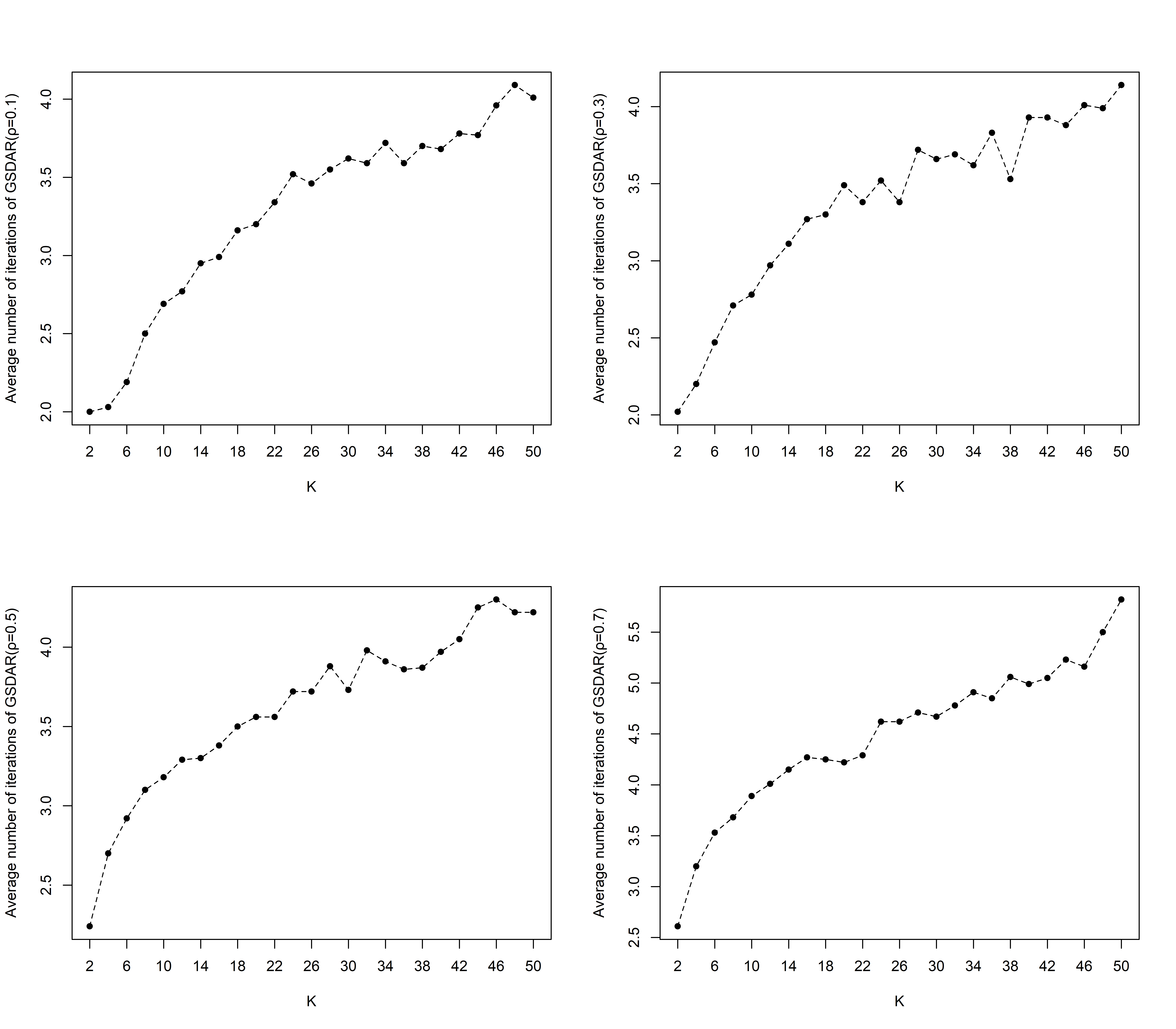
Figure 1: The average number of iterations of GSDAR as K increases

As shown in Fig. 1, the average number of iterations of the GSDAR algorithm increases as the sparsity level increases from 2 to 50 for every $\rho$. Even the sparsity level $K$ is 50, the average number of iterations is only 4 when the correlation $\rho$ is 0.1, 0.3, and 0.5, and is nearly 5.5 when the correlation $\rho$ is 0.7. It illustrates that our approach converges fast.

Table 5: Description of four real data sets

Data name	$n$ samples	$p$ features	training size $n_{1}$	testing set $n_{2}$
colon-cancer	62	2000	62	0
duke breast-cancer	42	7129	38	4
gisette	7000	5000	6000	1000
leukemia	72	7129	38	34

Table 6: Classification accuracy rate

Data name	GSDAR	AGSDAR	Lasso	MCP
colon-cancer	98.39%	96.77%	90.32%	85.48%
duke breast-cancer	1	1	1	25%
gisette	54.10%	56.30%	51.30%	59.90%
leukemia	91.18%	94.12%	91.17%	94.11%

5.4 Real data example

Analysing biological data using sparse learning methods is a hot topic [8, 18, 3, 13, 27]. We demonstrate the performance of the proposed methods GSDAR and AGSDAR with four real data: colon-cancer, duke breast-cancer, gisette and leukemia, which are exhaustively described in Table 5 and can be downloaded from https://www.csie.ntu.edu.tw/~cjlin/libsvmtools/datasets/. Besides, colon-cancer, duke breast-cancer and leukemia have been normalized such that the mean is $0$ and variance is 1, and the values $-1$s of response variable $y$ are replaced by $0$. Logistic regression model seeks to classify, then we get the classification accuracy rate, and compare the classification accuracy rate of the proposed methods with Lasso and MCP based on these real data sets. Let $T=0.5n/\log(n)$ in GSDAR, and implement the AGSDAR, Lasso and MCP by the same way as depicted in Section 5. When the data set has no testing data, we get the classification accuracy rate through the training set itself. The results are showed in Table 6, which indicates that the classification accuracy rates of GSDAR and AGSDAR are comparable to that of Lasso and MCP. As a result, the prosed methods are effective in colon-cancer, duke breast-cancer, gisette and leukemia data sets.

6 Conclusion

We extend the support detection and root finding (SDAR) algorithm to estimation in high-dimensional GLMs, then we get the GSDAR algorithm. GSDAR algorithm is also a constructive approach for fitting sparse, high-dimensional GLMs. In theory, we get $\ell_{\infty}$ optimal error bound for the sequence generated by GSDAR algorithm under some regular conditions. Further, we can get the oracle estimator, if the target signal is detectable with a high probability. We propose the AGSDAR algorithm, one adaptive version of GSDAR, to handle the problem of unknown sparsity level. Numerical results compared with Lasso and MCP on simulations and real data show GSDAR algorithm and AGSDAR algorithm are fast and stable and accurate.

For further research, we will extend GSDAR to solve structured sparsity learning problems [2, 11] with general convex losses or to problems related to deep neural networks (DNNs) [25, 15, 17].

Appendix A Appendix

In the appendix, we will show the proofs of the theoretical results.

A.1 Proof of Lemma 2.1

Proof.

Let $L_{\lambda}(\bm{\beta})=\mathcal{L}(\bm{\beta})+\lambda\|\bm{\beta}\|_{0}$. Assume $\bm{\beta}^{\diamond}$ is a global minimizer of $L_{\lambda}(\bm{\beta})$ and $\mbox{\bf d}^{\diamond}=-\nabla\mathcal{L}(\bm{\beta}^{\diamond})$. Then by Theorem 10.1 in [24], we have

$$\textbf{0}\in\nabla\mathcal{L}(\bm{\beta}^{\diamond})+\lambda\partial\|\bm{\beta}^{\diamond}\|_{0},$$ (7)

where $\partial\|\bm{\beta}^{\diamond}\|_{0}$ denotes the limiting subdifferential (see Definition 8.3 in [24]) of $\|\cdot\|_{0}$ at $\bm{\beta}^{\diamond}$. Let $\mbox{\bf d}^{\diamond}=-\nabla\mathcal{L}(\bm{\beta}^{\diamond})$ and define $G(\bm{\beta})=\frac{1}{2}\|\bm{\beta}-(\bm{\beta}^{\diamond}+\mbox{\bf d}^{\diamond})\|^{2}+\lambda\|\bm{\beta}\|_{0}$. Since (7) is equivalent to

$$\textbf{0}\in\bm{\beta}^{\diamond}-(\bm{\beta}^{\diamond}+\mbox{\bf d}^{\diamond})+\lambda\partial\|\bm{\beta}^{\diamond}\|_{0},$$

we deduce that $\bm{\beta}^{\diamond}$ is a KKT point of $G(\bm{\beta})$. Then $\bm{\beta}^{\diamond}=H_{\lambda}(\bm{\beta}^{\diamond}+\mbox{\bf d}^{\diamond})$ follows from the result that the KKT poits of $G$ is coincide with its coordinate-wise minimizer [9]. Conversely, suppose $\bm{\beta}^{\diamond}$ and $\mbox{\bf d}^{\diamond}$ satisfy (3), then $\bm{\beta}^{\diamond}$ is a local minimizer of $L_{\lambda}(\bm{\beta})$. To show $\bm{\beta}^{\diamond}$ is a local minimizer of $L_{\lambda}(\bm{\beta})$, we can assume h is small enough and $\|\mbox{\bf h}\|_{\infty}<\sqrt{2\lambda}$. Then we will show $L_{\lambda}(\bm{\beta}^{\diamond}+\mbox{\bf h})\geq L_{\lambda}(\bm{\beta}^{\diamond})$ in two case respectively.
Case1: $\mbox{\bf h}_{I^{\diamond}}\neq 0$.

$$\|\bm{\beta}^{\diamond}+\mbox{\bf h}\|_{0}=\|\bm{\beta}_{A^{\diamond}}^{\diamond}+\mbox{\bf h}_{A^{\diamond}}\|_{0}+\|\mbox{\bf h}_{I^{\diamond}}\|_{0},$$

$$\lambda\|\bm{\beta}^{\diamond}+\mbox{\bf h}\|_{0}-\lambda\|\bm{\beta}^{\diamond}\|_{0}=\lambda\|\bm{\beta}_{A^{\diamond}}^{\diamond}+\mbox{\bf h}_{A^{\diamond}}\|_{0}+\lambda\|\mbox{\bf h}_{I^{\diamond}}\|_{0}-\lambda\|\bm{\beta}_{A^{\diamond}}^{\diamond}\|_{0}.$$

Because $|\beta^{\diamond}_{i}|\geq\sqrt{2\lambda}$ for $i\in{A^{\diamond}}$ and $\|\mbox{\bf h}\|_{\infty}<\sqrt{2\lambda}$, we have

$$\lambda\|\bm{\beta}_{A^{\diamond}}^{\diamond}+\mbox{\bf h}_{A^{\diamond}}\|_{0}-\lambda\|\bm{\beta}_{A^{\diamond}}^{\diamond}\|_{0}=0,$$

$$\lambda\|\bm{\beta}^{\diamond}+\mbox{\bf h}\|_{0}-\lambda\|\bm{\beta}^{\diamond}\|_{0}=\lambda\|\mbox{\bf h}_{I^{\diamond}}\|_{0}>\lambda.$$

Therefore, we get

$$L_{\lambda}(\bm{\beta}^{\diamond}+\mbox{\bf h})-L_{\lambda}(\bm{\beta}^{\diamond})$$

$$=\sum_{i=1}^{n}[c(\mbox{\bf x}_{i}^{T}(\bm{\beta}^{\diamond}+\mbox{\bf h}))-c(\mbox{\bf x}_{i}^{T}\bm{\beta}^{\diamond})]-\mbox{\bf y}^{T}{\bf X}\mbox{\bf h}+\lambda\|\mbox{\bf h}_{I^{\diamond}}\|_{0}$$

$$>\sum_{i=1}^{n}[c(\mbox{\bf x}_{i}^{T}(\bm{\beta}^{\diamond}+\mbox{\bf h}))-c(\mbox{\bf x}_{i}^{T}\bm{\beta}^{\diamond})]-\mbox{\bf y}^{T}{\bf X}\mbox{\bf h}+\lambda$$

$$>0.$$

Let $m(\mbox{\bf h})=\sum_{i=1}^{n}[c(\mbox{\bf x}_{i}^{T}(\bm{\beta}^{\diamond}+\mbox{\bf h}))-c(\mbox{\bf x}_{i}^{T}\bm{\beta}^{\diamond})]-\mbox{\bf y}^{T}{\bf X}\mbox{\bf h}$, so $m(\mbox{\bf h})$ is a continuous function about h. As h is small enough and $\|\mbox{\bf h}\|_{\infty}<\sqrt{2\lambda}$, then $m(\mbox{\bf h})+\lambda>0$. Thus the last inequality holds.
Case2: $\mbox{\bf h}_{I^{\diamond}}=0$.

$$\lambda\|\bm{\beta}^{\diamond}+\mbox{\bf h}\|_{0}-\lambda\|\bm{\beta}^{\diamond}\|_{0}=\lambda\|\bm{\beta}_{A^{\diamond}}^{\diamond}+\mbox{\bf h}_{A^{\diamond}}\|_{0}-\lambda\|\bm{\beta}_{A^{\diamond}}^{\diamond}\|_{0}.$$

As $|\beta^{\diamond}_{i}|\geq\sqrt{2\lambda}$ for $i\in{A^{\diamond}}$ and $\|\mbox{\bf h}_{A^{\diamond}}\|_{\infty}<\sqrt{2\lambda}$, then we have

$$\lambda\|\bm{\beta}^{\diamond}+\mbox{\bf h}\|_{0}-\lambda\|\bm{\beta}^{\diamond}\|_{0}=\lambda\|\bm{\beta}_{A^{\diamond}}^{\diamond}+\mbox{\bf h}_{A^{\diamond}}\|_{0}-\lambda\|\bm{\beta}_{A^{\diamond}}^{\diamond}\|_{0}=0,$$

and

$$L_{\lambda}(\bm{\beta}^{\diamond}+\mbox{\bf h})-L_{\lambda}(\bm{\beta}^{\diamond})$$

$$=\sum_{i=1}^{n}[c(\mbox{\bf x}_{i}^{T}(\bm{\beta}^{\diamond}+\mbox{\bf h}))-c(\mbox{\bf x}_{i}^{T}\bm{\beta}^{\diamond})]-\mbox{\bf y}^{T}{\bf X}\mbox{\bf h}$$

$$=\sum_{i=1}^{n}[c(\mbox{\bf x}_{i(A^{\diamond})}^{T}(\bm{\beta}_{A^{\diamond}}^{\diamond}+\mbox{\bf h}_{A^{\diamond}}))-c(\mbox{\bf x}_{i(A^{\diamond})}^{T}\bm{\beta}_{A^{\diamond}}^{\diamond})]-\mbox{\bf y}^{T}{\bf X}_{A^{\diamond}}\mbox{\bf h}_{A^{\diamond}}$$

$$=\sum_{i=1}^{n}[c(\mbox{\bf x}_{i(A^{\diamond})}^{T}(\bm{\beta}_{A^{\diamond}}^{\diamond}+\mbox{\bf h}_{A^{\diamond}}))]-\mbox{\bf y}^{T}{\bf X}_{A^{\diamond}}(\bm{\beta}^{\diamond}_{A^{\diamond}}+\mbox{\bf h}_{A^{\diamond}})$$

$$\quad-\sum_{i=1}^{n}[c(\mbox{\bf x}_{i(A^{\diamond})}^{T}\bm{\beta}_{A^{\diamond}}^{\diamond})]+\mbox{\bf y}^{T}{\bf X}_{A^{\diamond}}\bm{\beta}^{\diamond}_{A^{\diamond}}$$

$$\geq 0.$$

As known that $\bm{\beta}_{A^{\diamond}}^{\diamond}\in\underset{\bm{\beta}_{A^{\diamond}}}{\mbox{argmin}}~{}\widetilde{\mathcal{L}}(\bm{\beta}_{A^{\diamond}})$, so the last inequality holds. In summary, $\bm{\beta}^{\diamond}$ is a local minimizer of $L_{\lambda}(\bm{\beta}^{\diamond})$. ∎

Lemma A.1.

Assume (C1) holds and $\|\bm{\beta}^{*}\|_{0}=K\leq T$. Denote $B^{k}=A^{k}\backslash A^{k-1}$. Then,

$$\|\nabla_{B^{k}}\mathcal{L}(\bm{\beta}^{k})\|_{1}\|\nabla_{B^{k}}\mathcal{L}(\bm{\beta}^{k})\|_{\infty}\geq 2L\zeta[\mathcal{L}(\bm{\beta}^{k})-\mathcal{L}(\bm{\beta}^{*})],$$

where $\zeta=\frac{|B^{k}|}{|B^{k}|+|A^{*}\backslash A^{k-1}|}$.

Proof.

Obviously, this lemma holds if $A^{k}=A^{k-1}$ or $\mathcal{L}(\bm{\beta}^{k})\leq\mathcal{L}(\bm{\beta}^{*})$. So we only prove the lemma by assuming $A^{k}\neq A^{k-1}$ and $\mathcal{L}(\bm{\beta}^{k})>\mathcal{L}(\bm{\beta}^{*})$. The condition (C1) indicates

$$\mathcal{L}(\bm{\beta}^{*})-\mathcal{L}(\bm{\beta}^{k})-\langle\nabla\mathcal{L}(\bm{\beta}^{k}),{\bm{\beta}^{*}-\bm{\beta}^{k}}\rangle$$

$$\quad\geq\frac{L}{2}\big{\|}\bm{\beta}^{*}-\bm{\beta}^{k}\big{\|}_{1}\big{\|}\bm{\beta}^{*}-\bm{\beta}^{k}\big{\|}_{\infty}.$$

Hence,

$$\langle-\nabla\mathcal{L}(\bm{\beta}^{k}),{\bm{\beta}^{*}-\bm{\beta}^{k}}\rangle$$

$$=\langle\nabla\mathcal{L}(\bm{\beta}^{k}),-\bm{\beta}^{*}\rangle$$

$$\geq\frac{L}{2}\big{\|}\bm{\beta}^{*}-\bm{\beta}^{k}\big{\|}_{1}\big{\|}\bm{\beta}^{*}-\bm{\beta}^{k}\big{\|}_{\infty}+\mathcal{L}(\bm{\beta}^{k})-\mathcal{L}(\bm{\beta}^{*})$$

$$\geq\sqrt{2L}\sqrt{\big{\|}\bm{\beta}^{*}-\bm{\beta}^{k}\big{\|}_{1}\big{\|}\bm{\beta}^{*}-\bm{\beta}^{k}\big{\|}_{\infty}}\sqrt{\mathcal{L}(\bm{\beta}^{k})-\mathcal{L}(\bm{\beta}^{*})}.$$

From the definition of $A^{k}$ and $A^{*}$, it is known that $B^{k}$ contains the first $|B^{k}|$-largest elements (in absolute value) of $\nabla\mathcal{L}(\bm{\beta}^{k})$, and $\mbox{supp}(\nabla\mathcal{L}(\bm{\beta}^{k}))\bigcap\mbox{supp}(\bm{\beta}^{*})=A^{*}\backslash A^{k-1}$. Thus, we have

$$\langle\nabla\mathcal{L}(\bm{\beta}^{k}),-\bm{\beta}^{*}\rangle \leq\frac{1}{\sqrt{\zeta}}\|\nabla_{B^{k}}\mathcal{L}(\bm{\beta}^{k})\|_{2}\|\bm{\beta}_{A^{*}\backslash A^{k-1}}^{*}\|_{2}$$

$$=\frac{1}{\sqrt{\zeta}}\|\nabla_{B^{k}}\mathcal{L}(\bm{\beta}^{k})\|_{2}\|(\bm{\beta}^{*}-\bm{\beta}^{k})_{A^{*}\backslash A^{k-1}}\|_{2}$$

$$\leq\frac{1}{\sqrt{\zeta}}\|\nabla_{B^{k}}\mathcal{L}(\bm{\beta}^{k})\|_{2}\|\bm{\beta}^{*}-\bm{\beta}^{k}\|_{2}$$

$$\leq\frac{1}{\sqrt{\zeta}}\sqrt{\|\nabla_{B^{k}}\mathcal{L}(\bm{\beta}^{k})\|_{1}\|\nabla_{B^{k}}\mathcal{L}(\bm{\beta}^{k})\|_{\infty}}$$

$$\quad\quad\times\sqrt{\|\bm{\beta}^{*}-\bm{\beta}^{k}\|_{1}\|\bm{\beta}^{*}-\bm{\beta}^{k}\|_{\infty}}.$$

Therefore,

$$\sqrt{2L}\sqrt{\mathcal{L}(\bm{\beta}^{k})-\mathcal{L}(\bm{\beta}^{*})}\leq\frac{1}{\sqrt{\zeta}}\sqrt{\|\nabla_{B^{k}}\mathcal{L}(\bm{\beta}^{k})\|_{1}\|\nabla_{B^{k}}\mathcal{L}(\bm{\beta}^{k})\|_{\infty}}.$$

In summary,

$$\|\nabla_{B^{k}}\mathcal{L}(\bm{\beta}^{k})\|_{1}\|\nabla_{B^{k}}\mathcal{L}(\bm{\beta}^{k})\|_{\infty}\geq 2L\zeta[\mathcal{L}(\bm{\beta}^{k})-\mathcal{L}(\bm{\beta}^{*})].$$

∎

Lemma A.2.

Assume (C1) holds with $0<U<\frac{1}{T}$, and $K\leq T$ in Algorithm 1. Then before Algorithm 1 terminates,

$$\mathcal{L}(\bm{\beta}^{k+1})-\mathcal{L}(\bm{\beta}^{*})\leq\xi[\mathcal{L}(\bm{\beta}^{k})-\mathcal{L}(\bm{\beta}^{*})],$$

where $\xi=1-\frac{2L(1-TU)}{T(1+K)}\in(0,1)$.

Proof.

Let $\Delta^{k}=\bm{\beta}^{k}-\nabla\mathcal{L}(\bm{\beta}^{k})$. The condition of (C1) indicates

$$\mathcal{L}(\Delta^{k+1}|_{A^{k+1}})-\mathcal{L}(\bm{\beta}^{k+1})\leq\langle\nabla\mathcal{L}(\bm{\beta}^{k+1}),\Delta^{k+1}|_{A^{k+1}}-\bm{\beta}^{k+1}\rangle$$

$$\quad\quad\quad\quad+\frac{U}{2}\big{\|}\Delta^{k+1}|_{A^{k+1}}-\bm{\beta}^{k+1}\big{\|}_{1}\big{\|}\Delta^{k+1}|_{A^{k+1}}-\bm{\beta}^{k+1}\big{\|}_{\infty}.$$

On the one hand, by the definition of $\bm{\beta}^{k+1}$ and $\nabla\mathcal{L}(\bm{\beta}^{k+1})$, we have

$$\langle\nabla\mathcal{L}(\bm{\beta}^{k+1}),\Delta^{k+1}|_{A^{k+1}}-\bm{\beta}^{k+1}\rangle$$

$$=\langle\nabla\mathcal{L}(\bm{\beta}^{k+1}),\Delta^{k+1}|_{A^{k+1}}\rangle$$

$$=\langle\nabla_{A^{k+1}}\mathcal{L}(\bm{\beta}^{k+1}),\Delta_{A^{k+1}}^{k+1}\rangle$$

$$=\langle\nabla_{A^{k+1}\backslash A^{k}}\mathcal{L}(\bm{\beta}^{k+1}),\Delta_{A^{k+1}\backslash A^{k}}^{k+1}\rangle.$$

Further, we also have

$$\big{\|}\Delta^{k+1}|_{A^{k+1}}-\bm{\beta}^{k+1}\big{\|}_{1}$$

$$=\big{\|}\Delta^{k+1}|_{A^{k+1}\backslash A^{k}}+\Delta^{k+1}|_{A^{k+1}\bigcap A^{k}}$$

$$\quad\quad-\bm{\beta}^{k+1}|_{A^{k+1}\bigcap A^{k}}-\bm{\beta}^{k+1}|_{A^{k}\backslash A^{k+1}}\big{\|}_{1}$$

$$=\big{\|}\Delta_{A^{k+1}\backslash A^{k}}^{k+1}\big{\|}_{1}+\big{\|}\Delta_{A^{k+1}\bigcap A^{k}}^{k+1}-\bm{\beta}_{A^{k+1}\bigcap A^{k}}^{k+1}\big{\|}_{1}$$

$$\quad\quad+\big{\|}\bm{\beta}_{A^{k}\backslash A^{k+1}}^{k+1}\big{\|}_{1}$$

$$=\big{\|}\Delta_{A^{k+1}\backslash A^{k}}^{k+1}\big{\|}_{1}+\big{\|}\bm{\beta}_{A^{k}\backslash A^{k+1}}^{k+1}\big{\|}_{1},$$

and

$$\big{\|}\Delta^{k+1}|_{A^{k+1}}-\bm{\beta}^{k+1}\big{\|}_{\infty}$$

$$=\big{\|}\Delta^{k+1}|_{A^{k+1}\backslash A^{k}}+\Delta^{k+1}|_{A^{k+1}\bigcap A^{k}}$$

$$\quad\quad-\bm{\beta}^{k+1}|_{A^{k+1}\bigcap A^{k}}-\bm{\beta}^{k+1}|_{A^{k}\backslash A^{k+1}}\big{\|}_{\infty}$$

$$=\big{\|}\Delta_{A^{k+1}\backslash A^{k}}^{k+1}\big{\|}_{\infty}\bigvee\big{\|}\bm{\beta}_{A^{k}\backslash A^{k+1}}^{k+1}\big{\|}_{\infty},$$

where $a\bigvee b=\max\{a,b\}$. On the other hand, by the definition of $A^{k}$, $A^{k+1}$ and $\bm{\beta}^{k+1}$, we know that

$$|A^{k}\backslash A^{k+1}|=|A^{k+1}\backslash A^{k}|,\quad\Delta_{A^{k}\backslash A^{k+1}}^{k+1}=\bm{\beta}_{A^{k}\backslash A^{k+1}}^{k+1}.$$

By the definition of $A^{k+1}$, we can conclude that

$$\|\Delta_{A^{k}\backslash A^{k+1}}^{k+1}\|_{1}=\|\bm{\beta}_{A^{k}\backslash A^{k+1}}^{k+1}\|_{1}\leq\|\Delta_{A^{k+1}\backslash A^{k}}^{k+1}\|_{1},$$

$$\|\Delta_{A^{k+1}\backslash A^{k}}^{k+1}\|_{\infty}\bigvee\|\bm{\beta}_{A^{k}\backslash A^{k+1}}^{k+1}\|_{\infty}=\|\Delta_{A^{k+1}\backslash A^{k}}^{k+1}\|_{\infty}.$$

Due to $-\nabla_{A^{k+1}\backslash A^{k}}\mathcal{L}(\bm{\beta}^{k+1})=\Delta_{A^{k+1}\backslash A^{k}}^{k+1}$ and $U<\frac{1}{T}$, hence we can deduce that

$$\mathcal{L}(\Delta^{k+1}|_{A^{k+1}})-\mathcal{L}(\bm{\beta}^{k+1})$$

$$\leq\langle\nabla_{A^{k+1}\backslash A^{k}}\mathcal{L}(\bm{\beta}^{k+1}),\Delta_{A^{k+1}\backslash A^{k}}^{k+1}\rangle$$

$$\quad+U\big{\|}\Delta_{A^{k+1}\backslash A^{k}}^{k+1}\big{\|}_{1}\big{\|}\Delta_{A^{k+1}\backslash A^{k}}^{k+1}\big{\|}_{\infty}$$

$$\leq-(1/T-U)\big{\|}\nabla_{A^{k+1}\backslash A^{k}}\mathcal{L}(\bm{\beta}^{k+1})\big{\|}_{1}$$

$$\quad\times\big{\|}\nabla_{A^{k+1}\backslash A^{k}}\mathcal{L}(\bm{\beta}^{k+1})\big{\|}_{\infty}.$$

By the definition of $\bm{\beta}^{k+1}$, we can get

$$\mathcal{L}(\bm{\beta}^{k+1})-\mathcal{L}(\bm{\beta}^{k})$$

$$\leq\mathcal{L}(\Delta^{k}|_{A^{k}})-\mathcal{L}(\bm{\beta}^{k})$$

$$\leq-(1/T-U)\big{\|}\nabla_{A^{k+1}\backslash A^{k}}\mathcal{L}(\bm{\beta}^{k+1})\big{\|}_{1}$$

$$\quad\times\big{\|}\nabla_{A^{k+1}\backslash A^{k}}\mathcal{L}(\bm{\beta}^{k+1})\big{\|}_{\infty}.$$

Moreover, $\frac{|A^{*}\backslash A^{k-1}|}{|B^{k}|}\leq K$. By Lemma A.1, we have

$$\mathcal{L}(\bm{\beta}^{k+1})-\mathcal{L}(\bm{\beta}^{k})\leq-\frac{2L(1-TU)}{T(1+K)}[\mathcal{L}(\bm{\beta}^{k})-\mathcal{L}(\bm{\beta}^{*})].$$

Therefore, we have

$$\mathcal{L}(\bm{\beta}^{k+1})-\mathcal{L}(\bm{\beta}^{*})\leq\xi[\mathcal{L}(\bm{\beta}^{k})-\mathcal{L}(\bm{\beta}^{*})],$$

where $\xi=1-\frac{2L(1-TU)}{T(1+K)}\in(0,1)$. ∎

Lemma A.3.

Assume $\mathcal{L}$ satisfies (C1) and

$$\mathcal{L}(\bm{\beta}^{k+1})-\mathcal{L}(\bm{\beta}^{*})\leq\xi[\mathcal{L}(\bm{\beta}^{k})-\mathcal{L}(\bm{\beta}^{*})]$$

for all $k\geq 0$. Then,

$$\begin{split}\|\bm{\beta}^{k}-\bm{\beta}^{*}\|_{\infty}&\leq\sqrt{(K+T)(1+\frac{U}{L})}(\sqrt{\xi})^{k}\|\bm{\beta}^{0}-\bm{\beta}^{*}\|_{\infty}\\ &\quad+\frac{2}{L}\|\nabla\mathcal{L}(\bm{\beta}^{*})\|_{\infty}.\end{split}$$ (8)

Proof.

If $\|\bm{\beta}^{k}-\bm{\beta}^{*}\|_{\infty}<\frac{2\|\nabla\mathcal{L}(\bm{\beta}^{*})\|_{\infty}}{L}$, then (8) holds, so we only consider the case that $\|\bm{\beta}^{k}-\bm{\beta}^{*}\|_{\infty}\geq\frac{2\|\nabla\mathcal{L}(\bm{\beta}^{*})\|_{\infty}}{L}$. On the one hand, $\mathcal{L}$ satisfies (C1), then

$$\mathcal{L}(\bm{\beta}^{k})-\mathcal{L}(\bm{\beta}^{*})$$

$$\geq\langle\nabla\mathcal{L}(\bm{\beta}^{*}),\bm{\beta}^{k}-\bm{\beta}^{*}\rangle+\frac{L}{2}\big{\|}\bm{\beta}^{k}-\bm{\beta}^{*}\big{\|}_{1}\big{\|}\bm{\beta}^{k}-\bm{\beta}^{*}\big{\|}_{\infty}$$

$$\geq-\|\nabla\mathcal{L}(\bm{\beta}^{*})\|_{\infty}\|\bm{\beta}^{k}-\bm{\beta}^{*}\|_{1}+\frac{L}{2}\big{\|}\bm{\beta}^{k}-\bm{\beta}^{*}\big{\|}_{1}\big{\|}\bm{\beta}^{k}-\bm{\beta}^{*}\big{\|}_{\infty}.$$

Due to $\|\bm{\beta}^{k}-\bm{\beta}^{*}\|_{\infty}\geq\frac{2\|\nabla\mathcal{L}(\bm{\beta}^{*})\|_{\infty}}{L}$, then

$$(\|\bm{\beta}^{k}-\bm{\beta}^{*}\|_{1}-\|\bm{\beta}^{k}-\bm{\beta}^{*}\|_{\infty})(\frac{L}{2}\|\bm{\beta}^{k}-\bm{\beta}^{*}\|_{\infty}-\|\nabla\mathcal{L}(\bm{\beta}^{*})\|_{\infty})\geq 0.$$

Further, we can get

$$\frac{L}{2}\|\bm{\beta}^{k}-\bm{\beta}^{*}\|_{\infty}^{2}-\|\nabla\mathcal{L}(\bm{\beta}^{*})\|_{\infty}\|\bm{\beta}^{k}-\bm{\beta}^{*}\|_{\infty}-[\mathcal{L}(\bm{\beta}^{k})-\mathcal{L}(\bm{\beta}^{*})]\leq 0,$$

which is univariate quadratic inequality about $\|\bm{\beta}^{k}-\bm{\beta}^{*}\|_{\infty}$. Thus, by simple computation, we can get

$$\|\bm{\beta}^{k}-\bm{\beta}^{*}\|_{\infty}\leq\sqrt{\frac{2\max\{\mathcal{L}(\bm{\beta}^{k})-\mathcal{L}(\bm{\beta}^{*}),0\}}{L}}+\frac{2\|\nabla\mathcal{L}(\bm{\beta}^{*})\|_{\infty}}{L}.$$ (9)

On the other hand, because $\mathcal{L}$ satisfies (C1), then

$$\mathcal{L}(\bm{\beta}^{0})-\mathcal{L}(\bm{\beta}^{*})$$

$$\leq\langle\nabla\mathcal{L}(\bm{\beta}^{*}),\bm{\beta}^{0}-\bm{\beta}^{*}\rangle+\frac{U}{2}\big{\|}\bm{\beta}^{0}-\bm{\beta}^{*}\big{\|}_{1}\big{\|}\bm{\beta}^{0}-\bm{\beta}^{*}\big{\|}_{\infty}$$

$$\leq\big{\|}\nabla\mathcal{L}(\bm{\beta}^{*})\big{\|}_{\infty}\big{\|}\bm{\beta}^{0}-\bm{\beta}^{*}\big{\|}_{1}+\frac{U}{2}\big{\|}\bm{\beta}^{0}-\bm{\beta}^{*}\big{\|}_{1}\big{\|}\bm{\beta}^{0}-\bm{\beta}^{*}\big{\|}_{\infty}$$

$$\leq(K+T)\big{\|}\bm{\beta}^{0}-\bm{\beta}^{*}\big{\|}_{\infty}(\|\nabla\mathcal{L}(\bm{\beta}^{*})\big{\|}_{\infty}+\frac{U}{2}\big{\|}\bm{\beta}^{0}-\bm{\beta}^{*}\big{\|}_{\infty}).$$

Then, we can get

$$\mathcal{L}(\bm{\beta}^{k})-\mathcal{L}(\bm{\beta}^{*}) \leq\xi[\mathcal{L}(\bm{\beta}^{k-1})-\mathcal{L}(\bm{\beta}^{*})]$$

$$\leq\xi^{k}[\mathcal{L}(\bm{\beta}^{0})-\mathcal{L}(\bm{\beta}^{*})]$$

$$\leq\xi^{k}(K+T)\big{\|}\bm{\beta}^{0}-\bm{\beta}^{*}\big{\|}_{\infty}$$

$$\quad\times(\|\nabla\mathcal{L}(\bm{\beta}^{*})\big{\|}_{\infty}+\frac{U}{2}\big{\|}\bm{\beta}^{0}-\bm{\beta}^{*}\big{\|}_{\infty})$$

$$\leq\frac{\xi^{k}(L+U)(K+T)}{2}\big{\|}\bm{\beta}^{0}-\bm{\beta}^{*}\big{\|}_{\infty}^{2}.$$

Hence, by (9), we have

$$\|\bm{\beta}^{k}-\bm{\beta}^{*}\|_{\infty} \leq\sqrt{(K+T)(1+\frac{U}{L})}(\sqrt{\xi})^{k}\|\bm{\beta}^{0}-\bm{\beta}^{*}\|_{\infty}$$

$$\quad+\frac{2}{L}\|\nabla\mathcal{L}(\bm{\beta}^{*})\|_{\infty}.$$

∎

Lemma A.4.

(Proof of Corollary 2 in [14]). Assume $x_{ij}^{,}s$ are sub-Gaussian and $n\gtrsim\log(p)$, then there exists universal constants $(c_{1},c_{2},c_{3})$ with $0<c_{i}<\infty$, $i=1,2,3$ such that

$$P\left(\|\nabla\mathcal{L}(\bm{\beta}^{*})\|_{\infty}\geq c_{1}\sqrt{\frac{\log(p)}{n}}\right)\leq c_{2}\exp(-c_{3}\log(p)).$$

A.2 Proof of Theorem 3.1

Proof.

By Lemma A.2, we have

$$\mathcal{L}(\bm{\beta}^{k+1})-\mathcal{L}(\bm{\beta}^{*})\leq\xi[\mathcal{L}(\bm{\beta}^{k})-\mathcal{L}(\bm{\beta}^{*})],$$

where

$$\xi=1-\frac{2L(1-TU)}{T(1+K)}\in(0,1).$$

So the conditions of Lemma A.3 are satisfied. Taking $\bm{\beta}^{0}=\textbf{0}$, we can get

$$\|\bm{\beta}^{k}-\bm{\beta}^{*}\|_{\infty}$$

$$\leq\sqrt{(K+T)(1+\frac{U}{L})}(\sqrt{\xi})^{k}\|\bm{\beta}^{*}\|_{\infty}+\frac{2}{L}\|\nabla\mathcal{L}(\bm{\beta}^{*})\|_{\infty}.$$

By Lemma A.4, then there exists universal constants $(c_{1},c_{2},c_{3})$ defined in Lemma A.4, with at least probability $1-c_{2}\exp(-c_{3}\log(p))$, we have

$$\|\bm{\beta}^{k}-\bm{\beta}^{*}\|_{\infty}$$

$$\leq\sqrt{(K+T)(1+\frac{U}{L})}(\sqrt{\xi})^{k}\|\bm{\beta}^{*}\|_{\infty}+\frac{2c_{1}}{L}\sqrt{\frac{\log(p)}{n}}.$$ (10)

Some algebra shows that

$$\|\bm{\beta}^{k}-\bm{\beta}^{*}\|_{\infty}\leq\mathcal{O}(\sqrt{\frac{\log(p)}{n}})$$

by taking $k\geq\mathcal{O}(\log_{\frac{1}{\xi}}\frac{n}{\log(p)})$ in (A.2). Then, the proof is complete. ∎

A.3 Proof of Theorem 3.2

Proof.

(A.2) and assumption (C2) and some algebra shows that that

$$\|\bm{\beta}^{k}-\bm{\beta}^{*}\|_{\infty}$$

$$\leq\sqrt{(K+T)(1+\frac{U}{L})}(\sqrt{\xi})^{k}\|\bm{\beta}^{*}\|_{\infty}+\frac{2}{3}\|\bm{\beta}^{*}_{A^{*}}\|_{\min}$$

$$<\|\bm{\beta}^{*}_{A^{*}}\|_{\min},$$

if $k>\log_{\frac{1}{\xi}}9(T+K)(1+\frac{U}{L})r^{2}.$ This implies that $A^{*}\subseteq A^{k}$. ∎

References

- [1] P. Breheny and J. Huang. Coordinate descent algorithms for nonconvex penalized regression, with applications to biological feature selection. The annals of applied statistics, 5(1):232, 2011.
- [2] P. Breheny and J. Huang. Group descent algorithms for nonconvex penalized linear and logistic regression models with grouped predictors. Statistics and Computing, 25(2):173–187, 2015.
- [3] J. Cai and X. Huang. Modified sparse linear-discriminant analysis via nonconvex penalties. IEEE Transactions on Neural Networks and Learning Systems, 29(10):4957–4966, 2018.
- [4] J. Fan and R. Li. Variable selection via nonconcave penalized likelihood and its oracle properties. Journal of the American statistical Association, 96(456):1348–1360, 2001.
- [5] J. Fan and J. Lv. Sure independence screening for ultrahigh dimensional feature space. Journal of the Royal Statistical Society: Series B (Statistical Methodology), 70(5):849–911, 2008.
- [6] J. Friedman, T. Hastie, and R. Tibshirani. Regularization paths for generalized linear models via coordinate descent. Journal of statistical software, 33(1):1, 2010.
- [7] J. Ge, X. Li, H. Jiang, H. Liu, T. Zhang, M. Wang, and T. Zhao. Picasso: A sparse learning library for high dimensional data analysis in R and Python. Journal of Machine Learning Research, 20(44):1–5, 2019.
- [8] B. Gu and V. S. Sheng. A solution path algorithm for general parametric quadratic programming problem. IEEE Transactions on Neural Networks and Learning Systems, 29(9):4462–4472, 2017.
- [9] J. Huang, Y. Jiao, B. Jin, J. Liu, X. Lu, and C. Yang. A unified primal dual active set algorithm for nonconvex sparse recovery. Statistical Science, Accepted.
- [10] J. Huang, Y. Jiao, Y. Liu, and X. Lu. A constructive approach to l 0 penalized regression. The Journal of Machine Learning Research, 19(1):403–439, 2018.
- [11] Y. Jiao, B. Jin, and X. Lu. Group sparse recovery via the penalty: theory and algorithm. IEEE Transactions on Signal Processing, 65(4):998–1012, 2017.
- [12] X. Li, L. Yang, J. Ge, J. Haupt, T. Zhang, and T. Zhao. On quadratic convergence of DC proximal Newton algorithm in nonconvex sparse learning. In Advances in Neural Information Processing Systems, pages 2742–2752, 2017.
- [13] X. Li, H. Zhang, R. Zhang, Y. Liu, and F. Nie. Generalized uncorrelated regression with adaptive graph for unsupervised feature selection. IEEE Transactions on Neural Networks and Learning Systems, 30(5):1587–1595, 2019.
- [14] P.-L. Loh and M. J. Wainwright. Regularized m-estimators with nonconvexity: Statistical and algorithmic theory for local optima. Journal of Machine Learning Research, 16:559–616, 2015.
- [15] C. Louizos, M. Welling, and D. P. Kingma. Learning sparse neural networks through regularization. In International Conference on Learning Representations, pages 1–13, 2018.
- [16] S. Luo and Z. Chen. Sequential lasso cum ebic for feature selection with ultra-high dimensional feature space. Journal of the American Statistical Association, 109(507):1229–1240, 2014.
- [17] R. Ma, J. Miao, L. Niu, and P. Zhang. Transformed regularization for learning sparse deep neural networks. 2019.
- [18] M. Mahmud, M. S. Kaiser, A. Hussain, and S. Vassanelli. Applications of deep learning and reinforcement learning to biological data. IEEE Transactions on Neural Networks and Learning Systems, 29(6):2063–2079, 2018.
- [19] P. McCullagh. Generalized linear models. Routledge, 2019.
- [20] L. Meier, S. Van De Geer, and P. Bühlmann. The group lasso for logistic regression. Journal of the Royal Statistical Society: Series B (Statistical Methodology), 70(1):53–71, 2008.
- [21] J. A. Nelder and R. W. Wedderburn. Generalized linear models. Journal of the Royal Statistical Society: Series A (General), 135(3):370–384, 1972.
- [22] Y. Nesterov. Gradient methods for minimizing composite functions. Mathematical Programming, 140(1):125–161, 2013.
- [23] M. Y. Park and T. Hastie. L1-regularization path algorithm for generalized linear models. Journal of the Royal Statistical Society: Series B (Statistical Methodology), 69(4):659–677, 2007.
- [24] R. T. Rockafellar and R. J.-B. Wets. Variational analysis, volume 317. Springer Science & Business Media, 2009.
- [25] S. Scardapane, D. Comminiello, A. Hussain, and A. Uncini. Group sparse regularization for deep neural networks. Neurocomputing, 241:81–89, 2017.
- [26] J. Shen and P. Li. On the iteration complexity of support recovery via hard thresholding pursuit. In Proceedings of the 34th International Conference on Machine Learning-Volume 70, pages 3115–3124. JMLR. org, 2017.
- [27] Y. Shi, J. Huang, Y. Jiao, and Q. Yang. A semismooth newton algorithm for high-dimensional nonconvex sparse learning. IEEE transactions on neural networks and learning systems, 2019.
- [28] R. Tibshirani. Regression shrinkage and selection via the lasso. Journal of the Royal Statistical Society: Series B (Methodological), 58(1):267–288, 1996.
- [29] S. A. Van de Geer et al. High-dimensional generalized linear models and the lasso. The Annals of Statistics, 36(2):614–645, 2008.
- [30] L. Wang, Y. Kim, and R. Li. Calibrating non-convex penalized regression in ultra-high dimension. Annals of statistics, 41(5):2505, 2013.
- [31] R. Wang, N. Xiu, and S. Zhou. Fast newton method for sparse logistic regression. arXiv preprint arXiv:1901.02768, 2019.
- [32] Z. Wang, H. Liu, and T. Zhang. Optimal computational and statistical rates of convergence for sparse nonconvex learning problems. Annals of statistics, 42(6):2164, 2014.
- [33] F. Ye and C.-H. Zhang. Rate minimaxity of the lasso and dantzig selector for the lq loss in lr balls. Journal of Machine Learning Research, 11(Dec):3519–3540, 2010.
- [34] X.-T. Yuan, P. Li, and T. Zhang. Gradient hard thresholding pursuit. Journal of Machine Learning Research, 18:166–1, 2017.
- [35] C.-H. Zhang et al. Nearly unbiased variable selection under minimax concave penalty. The Annals of statistics, 38(2):894–942, 2010.
- [36] C.-H. Zhang, T. Zhang, et al. A general theory of concave regularization for high-dimensional sparse estimation problems. Statistical Science, 27(4):576–593, 2012.
- [37] H. Zou and T. Hastie. Regularization and variable selection via the elastic net. Journal of the royal statistical society: series B (statistical methodology), 67(2):301–320, 2005.