Storage Placement and Sizing in a Distribution Grid with high PV-Generation

Abstract

With the increasing penetration of renewable resources in the distribution grid, the demand for alternatives to grid reinforcement measures rises. One possible solution is the use of battery systems to balance the power flow at crucial locations in the grid. Hereby the optimal location and size of the system has to be determined in regards of investment and grid stabilizing effect. In this paper the optimal placement and sizing of battery storage systems for grid stabilization in a small distribution grid in southern Germany with high PV- penetration is investigated and compared to a grid heuristical reinforcement strategy.

I Introduction

Nowadays, the rapid increment penetration of renewable energy resources into the distribution network can cause increased stress to the distribution system such as overvoltage situations or the exceeding of line ratings. Furthermore, the sustained need to establish a balance between energy demand and supply requires new solutions to enhance the reliable operation of the power system. Battery energy storage systems (BESS) are being proposed as a measure to enable the integration of more renewable energy generation into the distribution grid without the need for curtailing renewable generations or reinforcing the grid. The availability of storage also allows to maximize the energy efficiency, decrease the network losses as well as being able to deliver control or reserve energy to the grid. In this paper, the optimal placement and sizing of a battery energy storage system (BESS) for grid relief in a PV rich distribution grid are investigated. The method used is based on a linearized load flow method and will be tested with data from a real distribution grid.

II Literature Review

In the above mentioned context, battery storage systems connected to the distribution grid are the focus of numerous studies [1, 2, 3, 4, 5, 6]. Batteries can be used to reduce distribution system losses, removing existing hindrances to the integration of renewable distributed generation, contributing to voltage and frequency regulation [7, 8], facilitating peak shaving or decreasing the need of network expansion [9]. However, on account of the specific application and operational strategy, there is a need for an appropriate procedure to size and site the mentioned systems to minimize the costs and losses [10]. Additionally, the objective function in different methodologies implies considerable variation in outcomes of the cost-optimized placement and sizing of the BESS. Network structure, the renewable resource positions, and line-flow limits can also have impacts on optimal storage placement [11]. The mathematical techniques to calculate the problem of optimal siting and sizing the storage, which is in general non-convex and high dimensional, are classified into analytic techniques, artificial intelligence techniques, classical techniques or other assorted techniques [10, 12]. Motalleb et al. [13], proposed a heuristic method to find the optimal locations and capacity of multi-purpose battery energy storage system (BESS) taking account of distribution and transmission parts. Fossati et al. [14] found the optimal power capacity of a BESS that minimizes the operating cost of the microgrid based on genetic methods. A fuzzy expert system determines the power delivered or taken from the storage system. The advantage of the proposed algorithm is its easy adaptation to different types of microgrids. In [15], the economic optimal allocation of the energy storage is explored based on net present value using matrix-real-coded genetic algorithm techniques. The upside of this method is taking complete and overall design aspects into consideration. In [16, 17] the articles give a dissertation on how to minimize the sum of operation cost and to realize the optimal site and size the BESS based on particle swarm optimization (PSO). The objective in [18] is to enhance frequency control and reduce an operating cost by integrating the load shedding scheme with optimal sizing of BESS. The results depict the better performance of frequency control based on PSO in comparison with an analytic algorithm with load shedding scheme. However, the issue identified in heuristic methods is that they require huge calculations, and it is uncertain if they converge to the global optimal solution. In [10] a second order cone program (SOCP) convex relaxation of the power flow equations for optimal sizing and siting of BESS with a lower computational burden is presented. Hereby the objective function is formulated in two different manners: minimizing investment vs. power losses and minimizing investment vs. operational cost benefits in a variable price market. As discussed in [19] the load and generation balancing of interconnected renewable resources and energy storage can be controlled using a dynamic energy price. The problem is formulated in a stochastic dynamic program over a finite horizon with the aim to minimize the long-term average cost of used electricity as well as investment in storage.

III Cost Analysis

In this section follows an overview of the costs considered for battery placement and grid reinforcement. These are important to asses the optimal placement and sizing of battery systems correctly.

III-A Levelized Cost of Electricity

Looking at energy costs, the concept of levelized cost of energy (LCOE) is the center of attention as a significant practical as well as a transparent method for a cost and efficiency analysis which assists to establish a comparison with respect to costs between each individual alternative for energy generation. The key concept of LCOE, in a simplified manner, is the division of complete lifetime costs consisting of investments, operations, fuel outlay, local and financing conditions over electricity generation. A progressive research is conducted to elaborate the substantial attributes of LCOE, for instance, Fraunhofer ISE in [20] gives a dissertation to the present and future market evolution of clean resources such as PV, wind turbines and bio-gas and predicts the regarded LCOE for different resources till 2035 based on the scenarios defined for market expansion in Germany. The authors in [21] carried out research on Mauritius island and put the generation resources potential and island particular costs under consideration to find out the LCOE of technologies. The LCOE results from different resources are put into application to prioritize the energy systems in a cost-effective way. In [22], the article addresses three different types of PV-systems, and LCOE enables to obtain a comparison of these types under Morocco’s climate and helps the decision-making process.

III-B Levelized Cost of Energy Storage

The cost of energy storage plays an important role in economic decision making. In practice, determining a criterion to compute the storage cost is not easy. Further, in contrast with energy generation resources, energy storage technologies are being employed for different services such as a buffer in a dispatchable generation, peak shaving or to increase self-consumption. Therefore, the parameters which intervene in each case are different. An easy cost comparison of storage technologies is only possible when they are considered in a common location, application, and type. Battery storage has the property of being deployed in a distributed fashion. To determine the investment cost of a battery storage system, levelized cost of energy storage (LCOES) is measured in euro per charged $\mathrm{{\kilo}}\text{/}$ and depends on specific characteristics such as cycle lifespan, depth of discharge and round trip storage efficiency. The LCOES provides the customer a great insight into the price per kWh and helps to choose the appropriate battery by taking economic aspects into account.

The computation of the LCOES follows the definition of the LCOE formulation. For instance, in [23, 24], LCOES is formulated based on LCOE while instead of using fuel cost, charging cost is utilized and generated electricity is replaced by discharged electricity.

To estimate the total costs of energy storage placement correctly it is necessary to split up the costs into the power dependent and the capacity dependent costs. In [25] the relative component costs of battery storage systems are examined in a long-term storage market analysis, performed since 2014. Hereby, the total costs are split up into the cell costs, the power electronics, and the peripheral system costs. For residential systems, the relative costs for the power electronic components result in $42\text{\,}\mathrm{\char 37\relax}\text{/}$ of the total system costs. In this paper, it is assumed that the power electronics cost rise linearly with the rated system power of the battery. The estimated LCOES of the battery system were taken from [26] for the year 2019. The cost used for the battery placement are shown in Table I.

TABLE I: Battery Installation Costs For 2019.

type	perc.	costs/value
capacity	$42\text{\,}\mathrm{\char 37\relax}\text{/}$	$130$ $\mathrm{\per{\kilo}}\text{/}$
periphery	$28\text{\,}\mathrm{\char 37\relax}\text{/}$	$87$ $\mathrm{\per{\kilo}}\text{/}$
power electronics	$30\text{\,}\mathrm{\char 37\relax}\text{/}$	$93$ $\mathrm{\per{\kilo}}\text{/}$
installation	-	$20\,000$ $\mathrm{\text{€}}\text{/}\mathrm{batt}$
batt. lifetime	-	$10$ yr

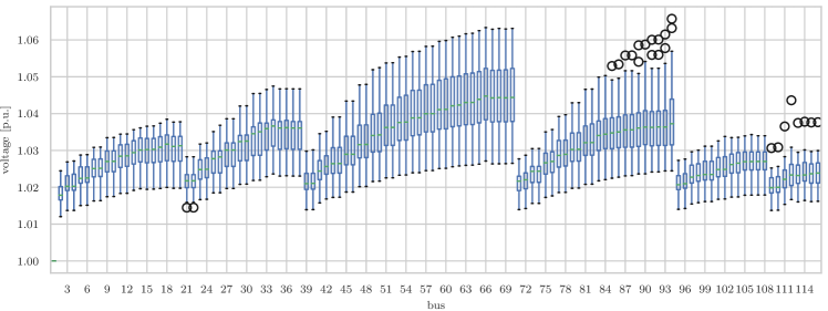
Figure 1: Voltage distribution for a day with high solar PV generation and no batter or energy curtailment. The voltage limit is 1.05 p.u., which is clearly passed

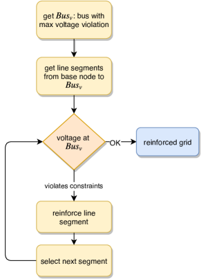
Figure 2: Flowchart of the heuristic grid reinforcement algorithm. The method shown above is repeated for all branches.

III-C Grid Reinforcement Costs

For the specific expansion costs, the two main shares for cables and installation costs are taken into account. The specific costs for the cables or lines depending on the line type are displayed in Table II.

However, the amounts for laying the cables vary greatly, depending on the condition of the ground. For arable land about $20\,000\text{\,}\mathrm{\per{\kilo}}\text{/}$ can be expected, but for stony ground the amount doubles ($40\,000\text{\,}\mathrm{\per{\kilo}}\text{/}$). In urban areas, where roads have to be rebuilt, the costs raise up to $80\,000\text{\,}\mathrm{\per{\kilo}}\text{/}$ [27]. For the installation of another cable in parallel, it is assumed that the installation costs increase by about $15\text{\,}\mathrm{\char 37\relax}\text{/}$ with each added line.

For the calculation of the annual costs, the useful lifespan of the lines still has to be determined. For underground cables, a lifespan of 40 years are generally assumed [28] and the normal operating life in accordance with the Electricity Grid Charges Ordinance is also 40 years [29].

TABLE II: Grid reinforcement costs.

line type	cost type	costs
0.4 kV, $4\times 50$ mm	installation	$60\,000$ $\mathrm{\per{\kilo}}\text{/}$
	acquisition	$3500$ $\mathrm{\per{\kilo}}\text{/}$
0.4 kV, $4\times 120$ mm	installation	$60\,000$ $\mathrm{\per{\kilo}}\text{/}$
	acquisition	$9900$ $\mathrm{\per{\kilo}}\text{/}$
0.4 kV, $4\times 150$ mm	installation	$60\,000$ $\mathrm{\per{\kilo}}\text{/}$
	acquisition	$12\,000$ $\mathrm{\per{\kilo}}\text{/}$
parallel line installation	installation	additional 15% of installation costs
Trafo, 630 kVA	total	$21\,000$ $\mathrm{\text{€}}\text{/}$

IV Input Data and Scenario

In this paper real measurement data (load and irradiation) from a German distribution grid with high PV penetration is used to investigate the effects of different storage placements and grid reinforcement scenarios.

IV-A PV Generation

To establish a worst case scenario for the grid loading induced by distributed generation a maximum PV penetration scenario was created. Hereby the roof area of the buildings as well as the azimuth and tilt angles were estimated to calculate the in-plane irradiance. It was assumed that the usable roof area for PV installations is 80 % share of the total roof area. With this information and the knowledge about the module size and type an estimate of the maximum possible PV-capacity was established which was called $P_{\text{PV, max}}$. To model the PV generation within the network the Python library pvlib [30] was used. This package includes all necessary functions to model the complete chain from the measured irradiance (GHI, DNI, DHI) to the inverter AC output power.

IV-B Simulation Scenario

Because of the computational complexity of the problem (distribution grid with 106 nodes), it is not possible to optimize in a single shot over one year. To capture the major grid stress for the battery placement, a worst case period has been selected from the measured data. The selected time-span is 3 days long and shows the highest consecutive net load (generation minus load) of the whole dataset.

Different simulation scenarios have been created to evaluate the dependency on voltage limitation and PV-penetration. The selected PV penetrations are $50\text{\,}\mathrm{\char 37\relax}\text{/}$ and $80\text{\,}\mathrm{\char 37\relax}\text{/}$ relative to $P_{\text{PV, max}}$. The maximum allowed voltage deviation are $3\text{\,}\mathrm{\char 37\relax}\text{/}$ and $5\text{\,}\mathrm{\char 37\relax}\text{/}$ from the nominal voltage.

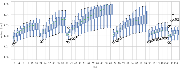
Figure 3: Voltage distribution for a day with high solar PV generation and one installed battery. In this case the voltage limit is obeyed at all nodes. The algorithm selected a battery placement at bus 65 and 93 to avoid voltage limit violations.

V Approach

In this section we will briefly describe the methods we used for the automated grid reinforcement and the battery placement algorithm. As the specific goal of the paper is to compare optimal battery placement with grid reinforcement alternatives such as curtailment of renewable generation to relax the grid stress are not taken into account.

V-A Grid Reinforcement

The grid reinforcement was calculated with a heuristic approach. Hereby the critical nodes of each branch are identified and the grid is reinforced until the given voltage limits are met at the corresponding nodes. The procedure of the algorithm is shown in Fig 2. The algorithm chooses always the cheapest option for the reinforcement based on the costs shown in Table II. Hereby it is also evaluated whether it is cheaper to install multiple smaller lines in parallel or to install a larger line.

V-B Battery Sizing and Placement

The algorithm is based on a linearized loadflow method presented in [31] and the optimization framework which is used in [32]. The time resolution of the algorithm is 1 hour. This can be justified with the properties of the battery system: The battery capacity is larger than the 1h times the max. rated power of the battery. Furthermore, the reaction time of the battery is very fast. Therefore the battery can compensate for the fluctuations within this hour and the average power over this time span can be used for the optimization. The simulation period as mentioned before is three days. Therefore multiple charging cycles are captured. This implies that the possibility to discharge the battery before the next cycle is ensured by the algorithm. Otherwise, the optimal size of the battery can not be calculated correctly.

The optimization places the battery storage units based on the costs shown in Table I and at the same time calculates an optimized charge trajectory for the batteries. Furthermore, constraints can be included, e.g. the number of batteries the algorithm is allowed to place.

This can be shown by an example calculation: In Fig. 1 the voltage situation within the grid is shown for a day with high solar PV generation and without an installed battery nor curtailment of PV-generation. The voltage limit within the grid is 1.05 p.u., which is surpassed in two branches here. In Fig. 3 the result of the optimization allowing one battery and curtailment is shown: The voltage limits are obeyed at all times. The algorithm chose to place the battery at bus 65 with a size of 83 kWh. The size is determined with the help of the provided irradiation and load profiles.

VI Results

In this section, the results of the above-mentioned algorithms in the given simulation scenario are shown and evaluated.

VI-A Grid Reinforcement

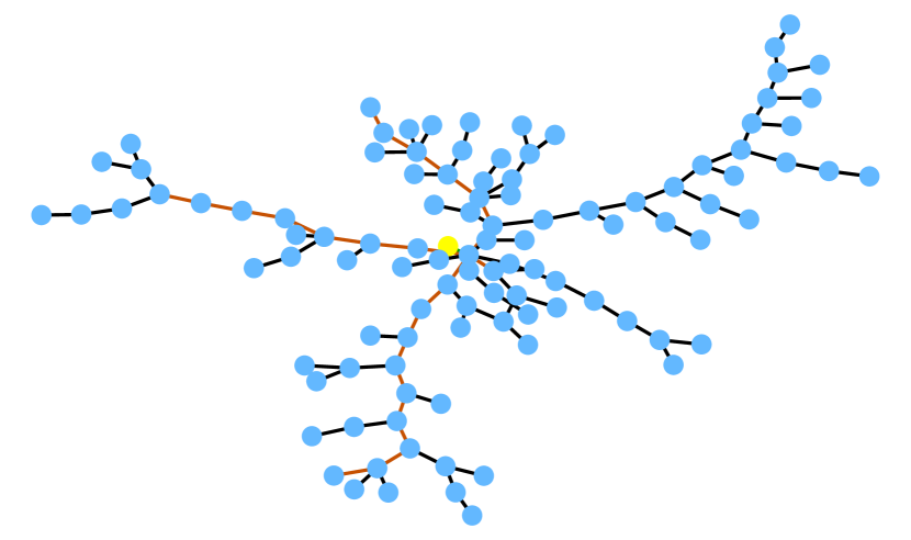
Figure 4: Graph diagram of the reinforced grid. The yellow node indicates the transformer and all the blue nodes are busses. The red edges indicate reinforced line segments.

TABLE III: Example Result of the Grid Reinforcement Algorithm: Overview of the installed assets and costs

from bus	to bus	n parallel	type	cost [k€]
$1$	$105$	$2$	NAYY $4\times 120$ SE	$109.5$
$1$	$73$	$2$	NAYY $4\times 120$ SE	$109.5$
$1$	$106$	$3$	NAYY $4\times 120$ SE	$131.1$
$2$	$28$	$1$	NAYY $4\times 120$ SE	$87.9$
$2$	$104$	$2$	NAYY $4\times 120$ SE	$109.5$
$3$	$61$	$1$	NAYY $4\times 120$ SE	$87.9$
$3$	$73$	$2$	NAYY $4\times 120$ SE	$109.5$
$6$	$43$	$1$	NAYY $4\times 50$ SE	$81.5$
$6$	$68$	$2$	NAYY $4\times 120$ SE	$109.5$
$28$	$29$	$1$	NAYY $4\times 50$ SE	$81.5$
$29$	$30$	$1$	NAYY $4\times 50$ SE	$81.5$
$50$	$57$	$1$	NAYY $4\times 120$ SE	$87.9$
$50$	$61$	$1$	NAYY $4\times 120$ SE	$87.9$
$56$	$57$	$1$	NAYY $4\times 120$ SE	$87.9$
$63$	$70$	$2$	NAYY $4\times 120$ SE	$109.5$
$63$	$69$	$2$	NAYY $4\times 120$ SE	$109.5$
$65$	$70$	$2$	NAYY $4\times 120$ SE	$109.5$
$65$	$106$	$1$	NAYY $4\times 120$ SE	$87.9$
$68$	$100$	$2$	NAYY $4\times 120$ SE	$109.5$
$69$	$100$	$2$	NAYY $4\times 120$ SE	$109.5$
$104$	$105$	$2$	NAYY $4\times 120$ SE	$109.5$

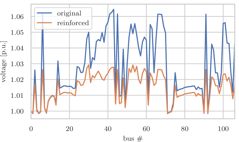
Figure 5: Voltage comparison of the original and the reinforced grid. In this case a voltage limit of 1.03 p.u. was used.

The grid reinforcement algorithm has shown to be computationally effective and at the same time sufficient to fulfill the task of calculating a cost-effective grid reinforcement. As it is a heuristic algorithm, the global optimality of the solution cannot be guaranteed. For radial distribution grids although a high-quality solution can be assumed. In Fig. 5 a comparison of the bus voltages of the original grid and the reinforced one is displayed. It can be seen that the algorithm added additional elements to reinforce the grid until the voltage limits are met at all nodes. The resulting reinforcement is shown in Fig. 4. The red edges of the graph indicate the reinforced line segments. Only the line segments with voltage problems were reinforced, in this case, three out of four branches.

The selection of the line types depends on the amount of reinforcement needed to meet the voltage constraints. In this example, the algorithm chose to use 18 times a cable of the type NAYY $4\times 120$ SE and three times the smaller NAYY $4\times 50$ SE (see Table III). As the transformer loading was still within the limits it was not replaced or reinforced.

VI-B Battery Placement

The results of the battery placement are summed up in Table IV for the different scenarios. For the scenario of a $50\text{\,}\mathrm{\char 37\relax}\text{/}$ penetration and a maximum voltage deviation of $5\text{\,}\mathrm{\char 37\relax}\text{/}$ relative to $V_{\text{nom}}$ no battery placement is needed. If the maximum voltage deviation is decreased to $3\text{\,}\mathrm{\char 37\relax}\text{/}$, 2 batteries have to be placed. For the scenario with $80\text{\,}\mathrm{\char 37\relax}\text{/}$ PV penetration a maximum voltage deviation of $5\text{\,}\mathrm{\char 37\relax}\text{/}$ relative to $V_{\text{nom}}$, the locations of the batteries stay almost the same as before, but the sizes increase. If the maximum voltage deviation is decreased to $3\text{\,}\mathrm{\char 37\relax}\text{/}$ in this case, a third battery has to be added. The results are additionally shown in Fig. 6 and Fig. 7. Here the placements for the $80\text{\,}\mathrm{\char 37\relax}\text{/}$ PV penetration and both voltage limitations are shown in a graph.

TABLE IV: Location and Size of the Battery

PV pen.	$\Delta\bm{\mathbf{V}}_{\text{max}}$	batt. 1		batt. 2		batt. 3
[$P_{\text{PV, max}}$]	[$V_{\text{nom}}$]	C [kWh]	bus #	C [kWh]	bus #	C [kWh]	bus #
50 $\mathrm{\char 37\relax}\text{/}$	5 $\mathrm{\char 37\relax}\text{/}$	-	-	-	-	-	-
	3 $\mathrm{\char 37\relax}\text{/}$	57	30	120	42	-	-
80 $\mathrm{\char 37\relax}\text{/}$	5 $\mathrm{\char 37\relax}\text{/}$	68	30	149	43	-	-
	3 $\mathrm{\char 37\relax}\text{/}$	497	29	426	45	116	59

In all cases the placement of the battery stays almost the same but varies just slightly by one or two buses. This indicates that the solution surface is relatively flat with respect to the battery position in the grid.

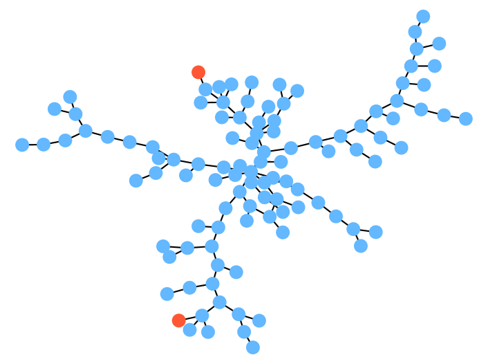
Figure 6: Battery placement for a PV penetration of $50\text{\,}\mathrm{\char 37\relax}\text{/}$ $P_{\text{PV, max}}$ and a maximum voltage deviation of $3\text{\,}\mathrm{\char 37\relax}\text{/}$.

Figure 7: Battery placement for a PV penetration of $80\text{\,}\mathrm{\char 37\relax}\text{/}$ $P_{\text{PV, max}}$ and a maximum voltage deviation of $3\text{\,}\mathrm{\char 37\relax}\text{/}$.

VI-C Comparison

In this section, the results of the battery placement and the grid reinforcement algorithm will be compared. In contrast to the previous section (VI-B) some constraint on the number of batteries to place are added to investigate the sensitivity on the number of batteries installed. Therefore two additional scenarios are introduced: one where the number of batteries is fixed to 5 and one with 10 batteries.

TABLE V: Investment Cost Comparison

PV pen.	$\Delta\bm{\mathbf{V}}_{\text{max}}$	grid reinf.	5 batt.	10 batt.	unconstr.
[$P_{\text{PV, max}}$]	[$V_{\text{nom}}$]	[k€]	[k€]	[k€]	[k€]	[n batt.]
50 %	3%	710	113	163	83	2
	5%	-	-	-	-	-
80 %	3%	1679	290	340	287	3
	5%	488	104	154	74	2

The results regarding the absolute investment costs are shown in Table V. The cheapest solution for the given scenarios is the installation of batteries to maintain the grid voltage stability. The costs increase with additional batteries, although the individual size of the batteries decreases. The most expensive option regarding the investment costs is grid reinforcement.

A more interesting comparison is the yearly costs. In this case, the maintenance costs for the battery as well as the grid are neglected, as they vary greatly. As mentioned before, the lifetime for the battery is assumed to be $10\text{\,}\mathrm{yr}\text{/}$ and the lifetime for the cables $40\text{\,}\mathrm{yr}\text{/}$. The results of this comparison are shown in Table VI. The result is similar to the investment costs, although the difference between the battery placement and the grid reinforcement is less pronounced.

TABLE VI: Yearly Cost Comparison (assumed lifetime: battery=10 yr, cable=40 yr)

PV pen.	$\Delta\bm{\mathbf{V}}_{\text{max}}$	grid reinf.	5 batt.	10 batt.	unconstr.
[$P_{\text{PV, max}}$]	[$V_{\text{nom}}$]	[k€]	[k€]	[k€]	[k€]	[n batt.]
50%	3%	18	11	16	8	2
	5%	0	0	0	0	0
80%	3%	42	29	34	29	3
	5%	12	10	15	7	2

VII Conclusion and Outlook

In this paper, we presented two algorithms: one for the automated placement and sizing of battery storage systems within a distribution grid and another algorithm for automated grid reinforcements. Both algorithms have shown to work and fulfill their task and avoid grid overloading for the suggested implementations. These algorithms can now be used to evaluate the possible solutions for distribution grids with congestion problems.

The results presented in this paper are only valid for the given scenario. However, the algorithm is capable of incorporating additional congestion management options such as the curtailment of renewable generation, load shifting, etc. These possibilities will be elaborated in a following paper.

References

- [1] B. Dunn, H. Kamath and J.-M. Tarascon “Electrical Energy Storage for the Grid: A Battery of Choices” In Science 334.6058, 2011, pp. 928–935 DOI: 10.1126/science.1212741
- [2] K.C. Divya and Jacob Østergaard “Battery energy storage technology for power systems—An overview” In Electric Power Systems Research 79.4, 2009, pp. 511–520 DOI: 10.1016/j.epsr.2008.09.017
- [3] Marc Beaudin, Hamidreza Zareipour, Anthony Schellenberglabe and William Rosehart “Energy storage for mitigating the variability of renewable electricity sources: An updated review” In Energy for Sustainable Development 14.4, 2010, pp. 302–314 DOI: 10.1016/j.esd.2010.09.007
- [4] Bruce S Dunn, Haresh Kamath and Jean-Marie Tarascon “Electrical energy storage for the grid: a battery of choices.” In Science 334 6058, 2011, pp. 928–35
- [5] Helder Lopes Ferreira et al. “Characterisation of electrical energy storage technologies” In Energy 53, 2013, pp. 288–298 DOI: 10.1016/j.energy.2013.02.037
- [6] Carlos Mateo et al. “Cost–benefit analysis of battery storage in medium-voltage distribution networks” In IET Generation, Transmission & Distribution 10.3, 2016, pp. 815–821 DOI: 10.1049/iet-gtd.2015.0389
- [7] Alexandre Oudalov, Daniel Chartouni and Christian Ohler “Optimizing a Battery Energy Storage System for Primary Frequency Control” In IEEE Transactions on Power Systems 22.3, 2007, pp. 1259–1266 DOI: 10.1109/TPWRS.2007.901459
- [8] S.K Aditya and D Das “Battery energy storage for load frequency control of an interconnected power system” In Electric Power Systems Research 58.3, 2001, pp. 179–185 DOI: 10.1016/S0378-7796(01)00129-8
- [9] P. Lazzeroni and M. Repetto “Optimal planning of battery systems for power losses reduction in distribution grids” In Electric Power Systems Research 167, 2019, pp. 94–112 DOI: 10.1016/j.epsr.2018.10.027
- [10] Etta Grover-Silva, Robin Girard and George Kariniotakis “Optimal sizing and placement of distribution grid connected battery systems through an SOCP optimal power flow algorithm” In Applied Energy 219, 2018, pp. 385–393 DOI: 10.1016/j.apenergy.2017.09.008
- [11] Subhonmesh Bose, Dennice F. Gayme, Ufuk Topcu and K. Chandy “Optimal placement of energy storage in the grid” In 2012 IEEE 51st IEEE Conference on Decision and Control (CDC) Maui, HI, USA: IEEE, 2012, pp. 5605–5612 DOI: 10.1109/CDC.2012.6426113
- [12] Prem Prakash and Dheeraj K. Khatod “Optimal sizing and siting techniques for distributed generation in distribution systems: A review” In Renewable and Sustainable Energy Reviews 57, 2016, pp. 111–130 DOI: 10.1016/j.rser.2015.12.099
- [13] Mahdi Motalleb, Ehsan Reihani and Reza Ghorbani “Optimal placement and sizing of the storage supporting transmission and distribution networks” In Renewable Energy 94, 2016, pp. 651–659 DOI: 10.1016/j.renene.2016.03.101
- [14] Juan P. Fossati, Ainhoa Galarza, Ander Martín-Villate and Luis Fontán “A method for optimal sizing energy storage systems for microgrids” In Renewable Energy 77, 2015, pp. 539–549 DOI: 10.1016/j.renene.2014.12.039
- [15] Changsong Chen et al. “Optimal Allocation and Economic Analysis of Energy Storage System in Microgrids” In IEEE Transactions on Power Electronics 26.10, 2011, pp. 2762–2773 DOI: 10.1109/TPEL.2011.2116808
- [16] Amirsaman Arabali, Mahmoud Ghofrani and Mehdi Etezadi-Amoli “Cost analysis of a power system using probabilistic optimal power flow with energy storage integration and wind generation” In International Journal of Electrical Power & Energy Systems 53, 2013, pp. 832–841 DOI: 10.1016/j.ijepes.2013.05.053
- [17] Ali Ahmadian et al. “Optimal probabilistic based storage planning in tap-changer equipped distribution network including PEVs, capacitor banks and WDGs: A case study for Iran” In Energy 112, 2016, pp. 984–997 DOI: 10.1016/j.energy.2016.06.132
- [18] Thongchart Kerdphol, Yaser Qudaih and Yasunori Mitani “Battery energy storage system size optimization in microgrid using particle swarm optimization” In IEEE PES Innovative Smart Grid Technologies, Europe Istanbul, Turkey: IEEE, 2014, pp. 1–6 DOI: 10.1109/ISGTEurope.2014.7028895
- [19] Pavithra Harsha and Munther Dahleh “Optimal Management and Sizing of Energy Storage Under Dynamic Pricing for the Efficient Integration of Renewable Energy” In IEEE Transactions on Power Systems 30.3, 2015, pp. 1164–1181 DOI: 10.1109/TPWRS.2014.2344859
- [20] Christoph Kost and Thomas Schlegl “Levelized Cost of Electricity- Renewable Energy Technologies”, 2018 URL: https://www.ise.fraunhofer.de/en/publications/studies/cost-of-electricity.html
- [21] Ryan P. Shea and Yatindra Kumar Ramgolam “Applied levelized cost of electricity for energy technologies in a small island developing state: A case study in Mauritius” In Renewable Energy 132, 2019, pp. 1415–1424 DOI: 10.1016/j.renene.2018.09.021
- [22] A. Allouhi et al. “Energetic, economic and environmental (3E) analyses and LCOE estimation of three technologies of PV grid-connected systems under different climates” In Solar Energy 178, 2019, pp. 25–36 DOI: 10.1016/j.solener.2018.11.060
- [23] Ilja Pawel “The Cost of Storage – How to Calculate the Levelized Cost of Stored Energy (LCOE) and Applications to Renewable Energy Generation” In Energy Procedia 46, 2014, pp. 68–77 DOI: 10.1016/j.egypro.2014.01.159
- [24] Andreas Belderbos, Erik Delarue and William D’haeseleer “Calculating the Levelized Cost of Electricity Storage?”, 2016
- [25] Marcus Müller et al. “Evaluation of Grid-Level Adaptability for Stationary Battery Energy Storage System Applications in Europe” In Journal of Energy Storage 9, 2017, pp. 1–11 DOI: 10.1016/j.est.2016.11.005
- [26] Vikas Bansal “Building A Bankable Solar + Energy Storage Project”, 2019, pp. 7
- [27] Linda Rupp, Marc Brunner and Stefan Tenbohlen “Einfluss dezentraler Wärmepumpen auf die Netzausbaukosten des Niederspannungsnetzes”, 2015 DOI: 10.17877/de290r-7269
- [28] Hofman and Oswald “Vergleich Erdkabel – Freileitung Im 110-kV-Hochspannungsbereich”, 2010
- [29] Klaus Heuck, Klaus-Dieter Dettmann and Detlef Schulz “Elektrische Energieversorgung Erzeugung, Übertragung und Verteilung elektrischer Energie für Studium und Praxis” OCLC: 1015863663 Wiesbaden: Vieweg+Teubner, 2010
- [30] William F., Clifford W. and Mark A. “Pvlib Python: A Python Package for Modeling Solar Energy Systems” In Journal of Open Source Software 3.29, 2018, pp. 884 DOI: 10.21105/joss.00884
- [31] B. Matthiss, M. Kraft and J. Binder “Fast Probabilistic Load Flow for Non-Radial Distribution Grids” In 2018 IEEE International Conference on Environment and Electrical Engineering and 2018 IEEE Industrial and Commercial Power Systems Europe (EEEIC / I CPS Europe), 2018, pp. 1–6 DOI: 10.1109/EEEIC.2018.8493678
- [32] Benjamin Matthiss, Arghavan Momenifarahani, Kay Ohnmeiss and Martin Felder “Influence of Demand and Generation Uncertainty on the Operational Efficiency of Smart Grids”, 2018 arXiv: http://arxiv.org/abs/1812.01886