Optimal FPE for non-linear 1d-SDE.
I: Additive Gaussian colored noise

Abstract

Many complex phenomena occurring in physics, chemistry, biology, finance, etc. Schadschneider et al. (2010) can be reduced, by some projection process, to a 1-d stochastic Differential Equation (SDE) for the variable of interest. Typically, this SDE is both non-linear and non-markovian, so a Fokker Planck equation (FPE), for the probability density function (PDF), is generally not obtainable. However, a FPE is desirable because it is the main tool to obtain relevant analytical statistical information such as stationary PDF and First Passage Time.

This problem has been addressed by many authors in the past (see among others Peacock-López et al. (1988); Tsironis and Grigolini (1988a); Fox (1986a)), but due to an incorrect use of the interaction picture (the standard tool to obtain a reduced FPE) previous theoretical results were incorrect, as confirmed by direct numerical simulation of the SDE.

We will show, in general, how to address the problem and we will derived the correct best FPE from a perturbation approach. The method followed and the results obtained have a general validity beyond the simple case of exponentially correlated Gaussian driving used here as an example; they can be applied even to non Gaussian drivings with a generic time correlation.

I Introduction

In the present work we are interested in non-linear 1-d SDEs of the form:

$$\dot{X}=-C(X)+\epsilon\xi(t).$$ (1)

where $X$ is the variable of interest, $-C(X)$ is the unperturbed drift field, $\xi(t)$ is the stochastic Gaussian perturbation with zero mean and autocorrelation function $\varphi(t)=\langle\xi(0)\xi(t)\rangle/\langle\xi^{2}\rangle$, the parameter $\epsilon$ controls the intensity of the perturbation, and $\langle...\rangle$ implies average over the $\xi$ realizations. The SDE in Eq. (1) is ubiquitous in many research fields Schadschneider et al. (2010).

The choice to consider the simple additive and Gaussian SDE is made because here we want to focus attention on a pitfalls that, in our opinion, must be considered and solved, when applying perturbation methods to dissipative systems. The extension to the case of multiplicative coloured noise, possible non-Gaussian, will be dealt with in a later work.

It is a standard result in statistical physics that when the stochastic forcing $\xi$ is a “white noise”, $\langle\xi(t)\xi(t^{\prime})\rangle=2\,\delta(t-t^{\prime})$, Eq. (1) leads to a flow for the Probability Density Function (PDF) $P(X;t)$ of the variable $X$ equivalent to the probability flow given by the following Fokker Planck Equation (FPE) (where $\partial_{X}:=\partial/\partial X$, $D_{0}=\epsilon^{2}.$):

$$\partial_{t}P(X;t) =\partial_{X}C(X)\,P(X;t)+D_{0}\,\partial_{X}^{2}P(X;t).$$ (2)

From Eq. (2), the stationary PDF is given by

$$P_{W,eq}(X)=\frac{1}{Z}e^{-\int^{X}\frac{C(y)}{D_{0}}\,\text{d}y}$$ (3)

where $Z$ is a normalization constant.

However, white noise is often an oversimplification of the real driving acting on a system of interest. Correlated noise (termed “colored” in the literature) is more common in continuous systems, and its importance has been recognized in a number of very different situations, like for instance statistical properties of dye lasers Zhu et al. (1986); Zhu (1993); Da-jin et al. (1989); Dong-cheng et al. (1999) chemical reaction rate Oliveira (1998); Fonseca et al. (1985); Bianucci and Grigolini (1992); Bianucci et al. (1990), optical bistability Lebreuilly et al. (2016); Horsthemke and Lefever (1984), large scale Ocean/Atmosphere dynamics Jin et al. (2007); Bianucci (2016) and many others.

We will assume that the stochastic process $\xi(t)$ is characterized by a “finite” correlation time $\tau$  and unitary intensity $\langle\xi^{2}\rangle\tau=1$. It is well known that if the unperturbed drift field is linear, regardless of the number of dimensions, the Gaussian property of a generic colored noise $\xi(t)$ is “linearly” transferred to the system of interest, so the FPE structure does not break (see, e.g., Adelman (1976); Bianucci et al. (1990)). On the contrary, in the case of non linear SDE and/or non Gaussian noise, for finite values of $\tau$ the FPE structure breaks down. This is the case of interest here, and the aim of this paper is to recover in some appropriate limits a FPE structure, obtaining an effective FPE with state dependent diffusion coefficient:

$$\partial_{t}P(X;t) =\partial_{X}C(X)\,P(X;t)+\partial_{X^{2}}^{2}D(X)P(X;t)$$ (4)

that, with a good approximation, could describe the evolution and the stationary properties of $P(X;t)$. Given $D(X)$, the stationary PDF of the FPE of Eq. (4) is then easily obtained

$$P_{s}(X)=\frac{1}{Z}\frac{e^{-\int^{X}\frac{C(Y)}{D(Y)}\text{d}Y}}{D(X)}$$ (5)

Several techniques have been developed to deal with the correlation time of the noise in nonlinear SDE, with the aim of eventually obtaining this effective FPE. They can be grouped in three main categories that correspond to three general techniques: the cumulant expansion technique Kubo (1962, 1963); Bianucci (2018), the functional-calculus approach Fox (1986b, a) (see also Peacock-López et al. (1988)) and the projection-perturbation methods (e.g., Grigolini and Marchesoni (1985); Grigolini (1989); Bianucci and Grigolini (1992); Bianucci (2015)). Each of these methods leads to a formally exact evolution equation for the PDF of the driven process, and the different descriptions are therefore equivalent. The exact formal results do not lend themselves to calculations nor give a FPE structure, therefore they require that approximations be made. The approximations made within these various formalisms involve truncations and/or partial resummations of infinite power series with respect to $\epsilon$ and $\tau$, which are typically the small parameters in the problem. Not surprisingly, it has been argued Peacock-López et al. (1988) that the effective FPE obtained from the different techniques are identical, if the same approximations are made (time scale separation, weak perturbation, Gaussian noise etc.). The results of the approximations can be grouped in two categories: the “Best Fokker Plank Equation” (BFPE) obtained by Lopez, West and Lindenberg Peacock-López et al. (1988) from a standard perturbation method, where $\epsilon$ is the small parameter and $\tau$ is finite but not limited, and the “Local Linearization Assumption” (LLA) FPE of Grigolini Tsironis and Grigolini (1988a) that coincides with the result of the functional-calculus approach of Fox Fox (1986b, a).

However, strangely enough, the BFPE often fails when compared with numerical simulations, even for relatively weak perturbations, while the LLA FPE usually works better. In Section IV we will comment briefly on this, leaving a more in-depth discussion to a later work.

In section II we will shortly review the perturbation approach that leads to the BFPE, stressing that care must be taken when using the interaction picture in strongly dissipative systems: the pitfalls we will point out are the sources of the defects of the original formulation of the BFPE. Section  III is the main section of the present work: we will show how to cure the shortcomings of the BFPE pointed out in section II. Section IV is devoted to a comparison with the LLA results. In section V we present the conclusions.

II The standard BFPE

From Eq. (1) it follows that, for any realization of the process $\xi(u)$, with $0\leq u\leq t$, the time-evolution of the PDF of the whole system, which we indicate with $P_{\xi}(X;t)$, satisfies the following PDE:

$$\partial_{t}P_{\xi}(X;t)={\cal L}_{a}\,P_{\xi}(X;t)+\epsilon\,\xi(t){\cal L}_{I}\,P_{\xi}(X;t)$$ (6)

in which the unperturbed Liouville operator ${\cal L}_{a}$ is

$${\cal L}_{a}:=\partial_{X}C(X)$$ (7)

and the Liouville perturbation operator is

$${\cal L}_{I}:=\partial_{X}.$$ (8)

A standard step of the perturbation method is to introduce the interaction representation, by which Eq. (6) becomes

$$\partial_{t}\tilde{P}_{\xi}(X;t)=\epsilon\xi(t)\,\tilde{\cal L}_{I}(t)\tilde{P}_{\xi}(X;t),$$ (9)

where

$$\tilde{P}_{\xi}(X;t):=e^{-{\cal L}_{a}t}P_{\xi}(X;t),$$ (10)

and

$$\tilde{\cal L}_{I}(t):=e^{-{\cal L}_{a}t}{\cal L}_{I}e^{{\cal L}_{a}t}=e^{-{\cal L}_{a}^{\times}t}[{\cal L}_{I}],$$ (11)

where, for any couple of operators ${\cal A}$ and ${\cal B}$, we have defined ${\cal A}^{\times}[{\cal B}]:=[{\cal A},{\cal B}]={\cal A}{\cal B}-{\cal B}{\cal A}$. The last step in Eq. (11) is easily proved by induction and it is known as the Hadamard’s lemma for exponentials of operators. In Bianucci (2018) $\tilde{\cal L}_{I}(t)$ of Eq. (11) is also called the Lie evolution of the operator ${\cal L}_{I}$ along the Liouvillian ${\cal L}_{a}$, for a time $-t$. For further use, we note that the Lie evolution of a product of operators is the product of the Lie evolution of the individual operators:

$$e^{{\cal A}^{\times}t}[{\cal B}{\cal C}]=e^{{\cal A}^{\times}t}[{\cal B}]\,e^{{\cal A}^{\times}t}[{\cal C}].$$

Integrating Eq. (9) and averaging over the realization of $\xi(t)$, we get

$$\tilde{P}(X;t)=\langle\overleftarrow{\exp}\left[\int_{0}^{t}du\;\xi(u)\tilde{\cal L}_{I}(u)\right]\rangle P(X;0)$$ (12)

where $\overleftarrow{\exp}[...]$ is the standard chronological ordered exponential (from right to left), $P(X;t):=\langle P_{\xi}(X;t)\rangle$ and we assumed that $P_{\xi}(X;0)=P(X;0)$, i.e. at the initial time $t=0$ $P_{\xi}(X;0)$ does not depend on the possible values of the process $\xi$, or that we wait long enough to make the initial conditions irrelevant. The r.h.s. of Eq. (9) can be considered as a sort of generalized moment generating function for the fluctuating operator $\xi(u)\tilde{\cal L}_{I}$ to which it is possible to associate a generalized cumulant generating function Bianucci (2018). Keeping up to the second generalized cumulants leads to the following result Bianucci (2018) (note that we use the assumption $\langle\xi^{2}\rangle\tau=1$, from which $\langle\xi^{2}\rangle=1/\tau$)

$$\partial_{t}\tilde{P}(X;t)=\epsilon^{2}\,\tilde{\cal L}_{I}(t)\int_{0}^{t}du\;\tilde{\cal L}_{I}(u)\varphi(t-u)P(X;t)$$ (13)

which coincides with the usual one obtained using a second order in $\epsilon,$ Zwanzig projection approach Bianucci (2015).

Getting rid of the interaction picture, from Eq. (13) we obtain

$$\partial_{t}{P}(X;t)$$

$$={\cal L}_{a}P(X;t)+\epsilon^{2}\,\partial_{X}\,\frac{1}{\tau}\int_{0}^{t}\mbox{d}u\,e^{{\cal L}_{a}^{\times}u}[\partial_{X}]\varphi(u){P}(X;t).$$ (14)

This is a standard result, in fact, as we have already stressed, it can be obtained with any perturbation approach, where $\epsilon$ is the small parameter (assuming a finite, but not necessary small, correlation time $\tau$). We have cited the generalized cumulant approach because it gives a sound justification of the second order truncation of the full series of generalized comulants Bianucci (2018)). The next step is to rewrite, if possible, Eq. (II) as the FPE of Eq.( 4)

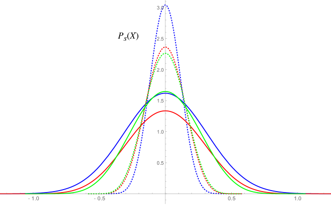
Figure 1: The case where $C(X)=\sinh(X)$, and $\langle\xi^{2}\rangle=1$, $\varphi(t)=\exp(-t/\tau)$, $\tau=0.8$ and $\epsilon=0.3$. The graphs are the PDFs obtained from Eq. (5), in which the state dependent diffusion coefficient $D(X)$ is evaluated from Eq. (II) supplemented with the series expansion of Eq. (II) truncated at the fifth order. The solid lines refer to even orders: zeroth (blue), second (red) and fourth (green) one. The dashed lines refer to odd orders: first (blue), third (red) and fifth (green) one.

To go from Eq. (II) to the FPE of Eq. (4), the crucial term is the operator $e^{{\cal L}_{a}^{\times}u}[\partial_{X}]$. In most papers using the Zwanzig projection method (e.g., Grigolini and Marchesoni (1985)), the explicit FPE is obtained from Eq. (II) assuming that $\tau$, identified with the decay time of the correlation function $\varphi(t)$, is much smaller than the time scale of the unperturbed dynamics driven by the Liouvillian ${\cal L}_{a}$. In this case it is possible to replace, in Eq. (II), the power expansion (note the shorthand $(\partial_{X}C(X)):=C^{\prime}(X)$)

$$e^{{\cal L}_{a}^{\times}u}[\partial_{X}] =\partial_{X}+[{\cal L}_{a},\partial_{X}]\,u+O(u^{2})$$

$$=\partial_{X}-\partial_{X}\,C^{\prime}(X)\,u+O(u^{2}).$$ (15)

that leads to a FPE with a state dependent diffusion coefficient, given by a series of “moments” of the time $u$, weighted with the correlation function $\varphi(u)$. However, such a series, as it is apparent from Eq. (II), contains secular terms and is (generally) not absolutely convergent. This is clearly shown in the example considered in Fig. 1. A way to avoid this problem is to solve, without approximations, the Lie evolution of the differential operator $\partial_{X}$ along the Liovillian ${\cal L}_{a}$. In Bianucci (2018) this was done for the general case of multidimensional systems and multiplicative forcing. In the present simpler one-dimensional case, recalling that ${\cal L}_{a}=\partial_{X}C(X)$, the Lie evolution of ${\partial_{X}}$, without approximations, can be obtained directly as follows:

$$e^{{\cal L}_{a}^{\times}u}[\partial_{X}]=e^{{\cal L}_{a}^{\times}u}[\partial_{X}C(X)\frac{1}{C(X)}]$$

$$=e^{{\cal L}_{a}^{\times}u}[{\cal L}_{a}]\,e^{{\cal L}_{a}^{\times}u}[\frac{1}{C(X)}]=\partial_{X}C(X)\frac{1}{C(X_{0}(X;-u))}$$ (16)

where $X_{0}(X;-u):=e^{{\cal L}_{a}^{\times}u}[X]=\left(e^{-{\cal L}_{a}^{+}u}X\right)$ is the unperturbed backward evolution, for a time $u$, of the variable of interest, starting from the $X$ position at the initial time $u=0$. In the second line of Eq. (II) we have used two trivial facts (see again Bianucci (2018) for details and generalizations):

• given two operators ${\cal A}$ and ${\cal B}$, ${\cal B}$ does not Lie-evolve along ${\cal A}$ when $[{\cal A},{\cal B}]=0$, thus $e^{{\cal L}_{a}^{\times}u}[{\cal L}_{a}]={\cal L}_{a}$,

• the Lie evolution along a deterministic (first order partial differential operator) Liouvillian of a regular function $C(X)$, is just the back-time evolution of $C(X)$ along the flow generated by the same Liouvillian:

  $$e^{{\cal L}_{a}^{\times}u}[C(X)]=C(X_{0}(X;-u)).$$ (17)

Inserting Eq. (II) in Eq. (II) we get, in a clear and straight way, the BFPE of Lopez, West and Lindenberg Peacock-López et al. (1988) :

$$\partial_{t}{P}(X;t)={\cal L}_{a}P(X;t)$$

$$+\epsilon^{2}\,\partial_{X}^{2}\,\frac{1}{\tau}C(X)\left(\int_{0}^{t}\mbox{d}u\,\frac{1}{C(X_{0}(X;-u))}\varphi(u)\right){P}(X;t),$$ (18)

namely, the FPE of Eq. (4) with the state and time dependent diffusion coefficient

$$D(X,t)_{BFPE}=\epsilon^{2}\frac{1}{\tau}C(X)\left(\int_{0}^{t}\mbox{d}u\,\frac{1}{C(X_{0}(X;-u))}\varphi(u)\right)\\$$ (19)

that, for large times, becomes

$$D(X,\infty)_{BFPE}=\epsilon^{2}\frac{1}{\tau}C(X)\left(\int_{0}^{\infty}\mbox{d}u\,\frac{1}{C(X_{0}(X;-u))}\varphi(u)\right).$$ (20)

For weak enough noise intensity $\epsilon$, the BFPE looks like the best possible approximation we can get from a perturbation approach to the SDE of Eq. (1). However, this is not the case: the diffusion coefficient in Eq. (20) turns out to be wrong, as we are going to show.

It is actually known that in many cases of interest the diffusion coefficient $D(X)_{BFPE}$, given in Eq. (20), becomes negative, giving rise to a non physical negative PDF. A simple example may serve for illustration. Let us consider the case in which $C(X)=\alpha\sinh(kX)$ and $\varphi(t)=\exp(-t/\tau)$, with $\alpha>0$. The corresponding SDE is related to a well known chemical reaction scheme, see Lindenberg and West (1983). A straightforward calculation leads to $C(X)/C(X_{0}(X;-u))=\cosh(\alpha ku)-\cosh(kX)\sinh(\alpha ku)$, which inserted in Eq. (20), for times $t>>\tau/(1-\alpha k\tau)$, gives ($\theta:=\alpha k\tau$)

$$D(X,\infty)_{BFPE}=\epsilon^{2}\,\frac{1-\theta\cosh(kX)}{1-\theta},$$ (21)

with the constraint $\theta<1$. From Eq. (21) we see that for $X=\pm\tilde{X}$, with $\tilde{X}:=\frac{\log\left(\sqrt{\theta^{2}-1}+\theta\right)}{k}$, the diffusion coefficient of the BFPE vanishes and for $|X|>\tilde{X}$ it is negative which is clearly unphysical. Using Eq. (21) in Eq. ( 5), we obtain the stationary PDF:

$$P_{s}(X)_{BFPE}=\frac{1}{Z_{BFPE}}\left(\frac{1-\theta\cosh(kX)}{1-\theta}\right)^{\frac{1-\theta^{2}-k^{2}\tau^{2}\epsilon^{2}}{k^{2}\tau\,\epsilon^{2}}}$$ (22)

that is affected by the same problem for $|X|>\tilde{X}$. The standard way to cure this flaw of the BFPE is to restrict the support of the PDF Lindenberg and West (1983); Peacock-López et al. (1988). In this case, for example, the first and the second derivatives of Eq. (22) vanish in $|X|=\tilde{X}$, therefore one could limit the support of the PDF of Eq. (22) to $X\in(-\tilde{X},\tilde{X})$. However, from Fig. 2 it is clear that by increasing $\epsilon$, the result of Eq. (22) does not agree well with that obtained from the numerical simulation of the SDE of Eq. (1). Only for very small values of $\tau\epsilon$ the result is good (i.e, when the width of the PDF is small compared to $2\tilde{X}$). The same problem is present when other drift fields $C(X)$ are considered: the case of $C(X)=X^{3}$ is shown in Appendix A, other examples can be found in the literature Masoliver et al. (1987); Tsironis and Grigolini (1988b, a); Grigolini et al. (1988)).

Figure 2: Solid black lines: the stationary PDF from the numerical simulation of the SDE of Eq. (1) with $C(X)=\alpha\sinh(kX)$ and $\alpha=k=1$. Dashed gray lines: the BFPE stationary PDF $P_{s}(X)_{BFPE}$ from Eq. (21), the interval $-\tilde{X}<X<\tilde{X}$ is the support of this PDF (see text). Dotted blue lines: the cBFPE stationary PDF $P_{s}(X)_{cBFPE}$ (discussed further down in this paper) obtained from Eq. (5) using $D(X)=D(X,\infty)_{cBFPE}$ of Eq. (III). Note how the BFPE PDF completely fails when, increasing $\epsilon$, the width of the PDF becomes comparable (or larger) than the interval width $2\tilde{X}$, whereas there is an excellent agreement between simulations and cBFPE PDF for $\tau$ and $\epsilon$ considered.

III The cured BFPE

We show in this section that the flaws of the BFPE are due to an incorrect implementation of the perturbation procedure, and we will cure this situation.

Note first that the possibly negative $D_{BFPE}$ value of Eq. (20) is due to the fact that the kernel of the integral can be negative for some $X$ values.

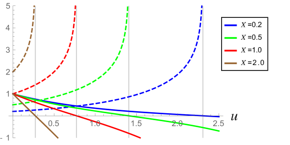
Figure 3: Case $C(X)=\sinh(X)$. Solid colored lines: the function $C(X)/C(X_{0}(X;-u))=\cosh(u)-\sinh(u)\cosh(X)$ for different initial positions $X_{0}(X;0)=X$. Dashed colored lines: the back time evolution $X_{0}(X;-u)=2\coth^{-1}\left(e^{-u}\coth\left(\frac{X}{2}\right)\right)$, for the same different initial values $X_{0}(X;0)=X$. Thin gray vertical lines: asymptotes at the corresponding time values $\bar{u}(X)=\log\left(\sqrt{\frac{\cosh(X)+1}{\cosh(X)-1}}\right)$. At the time value $\bar{u}(X)$ where the back time evolution $X_{0}(X;-u)$ diverges, the function $C(X)/C(X_{0}(X;-u))$ vanishes. For larger times it is a negative number.

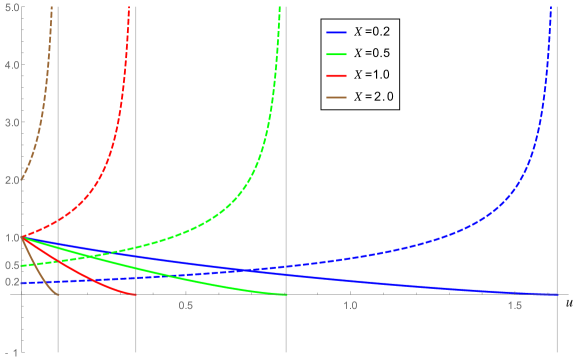
Figure 4: Case $C(X)=\alpha X^{3}$ with $\alpha=1$. Solid colored lines: the function $C(X)/C(X_{0}(X;-u))=e^{u/2}\left(-2X^{2}\sinh(u)-\sinh(u)+\cosh(u)\right)^{3/2}$ for different initial positions $X_{0}(X;0)=X$. Dashed colored lines: the back time evolution $X_{0}(X;-u)=X/\sqrt{-X^{2}+e^{-2u}(1+X^{2})}$, for the same initial values $X_{0}(X;0)=X$. Thin gray vertical lines: asymptotes at the corresponding time values $\bar{u}(X)=-\frac{1}{2}\log\left(\frac{X^{2}}{X^{2}+1}\right)$. At the times $\bar{u}$ when the back time evolution $X_{0}(X;-u)$ diverges, the function $C(X)/C(X_{0}(X;-u))$ vanishes, while for larger times it is a complex number.

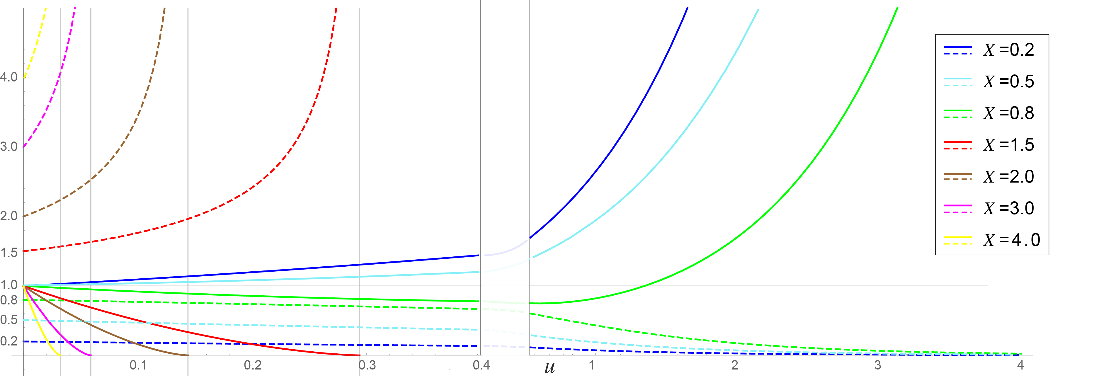
Figure 5: Case $C(X)=X+\alpha X^{3}$, $\alpha=1$. Solid colored lines: $C(X)/C(X_{0}(X;-u))=e^{-u}(\sqrt{\alpha\left(e^{2u}-1\right)X^{2}+1}\,)^{3}$ for different initial positions $X_{0}(X;0)=X$. Dashed colored lines: $X_{0}(X;-u)=e^{u}X/\sqrt{\alpha\left(e^{2u}-1\right)X^{2}+1}$ for the same initial values $X_{0}(X;0)=X$. Thin gray vertical lines: asymptotes at the corresponding time values $\bar{u}=\frac{1}{2}\log\left(\frac{\alpha X^{2}-1.}{\alpha X^{2}}\right)$. For $|X|<1$ the backward trajectories do not diverge at all and the function $C(X)/C(X_{0}(X;-u)$ is always positive.

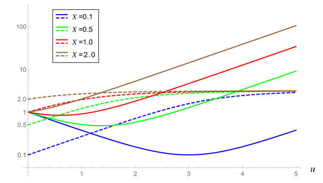
Figure 6: Semi-log plot for the case $C(X)=\alpha\sin(kX)$, $\alpha=k=1$. Solid colored lines: $C(X)/C(X_{0}(X;-u))=\cosh(k\alpha u)-\sinh(k\alpha u)\cos(kX)$ for different initial positions $X_{0}(X;0)=X$. Dashed colored lines: the back time evolution $X_{0}(X;-u)=2\cot^{-1}\left(e^{-k\alpha u}\cot\left(\frac{kX}{2}\right)\right)/k$, for the same initial values $X_{0}(X;0)=X$.

Considering once more the case of $C(X)=\alpha\sinh(kX)$, we see from Fig. 3, solid lines, that, after a given time $\bar{u}(X)$, the function $C(X)/C(X_{0}(X;-u))$ becomes negative. Note also that the larger the $X$ value, the shorter the time $\bar{u}(X)$. Thus, whatever the correlation decay time $\tau\in(0,1/\alpha k)$, there will always be a certain $\tilde{X}$ value such that $D(X,\infty)_{BFPE}$ of Eq. (20) is negative for $|X|>\tilde{X}$ (the greater the $\tau$ value, the smaller the $\tilde{X}$ value).

Depending on $C(X)$, we may have rather different scenario: for example, when $C(X)=X^{3}$ for $|X|>\tilde{X}$, the kernel of the $D(X,\infty)_{BFPE}$ of Eq. (20), turns out to be a complex number see Appendix A and Fig. 4. Therefore, in this case it would seem that the BFPE does not exist at all.

Other interesting examples are the case when $C(X)=X+\alpha X^{3}$ (see Fig. 5), where, depending on the initial $X$, the kernel can go negative ($|X>1|$) or stay positive ($|X<1|$); and the case when $C(X)=\alpha\sin(kX)$, where the kernel is always positive (see Fig. 6).

The shortcomings of the BFPE are however artifacts, introduced by an unapropriate use of the interaction picture, and they can be fixed.

When we go to the interaction picture and then return to the normal representation, we time evolve the variable of interest forth and back, along the flow generated by the $-C(X)$ drift field.

The backward evolution is indicated by $X_{0}=X_{0}(X;-u)$. Using Eq. (1) we can easily invert this relation, to get $u(X,X_{0})=\int_{X}^{X_{0}}\frac{1}{c(y)}\;dy$. We define the $X$ dependent time $\bar{u}(X)$ as the time it takes the unperturbed evolution, starting from $X$, to go to $X_{0}\rightarrow\infty$, namely $\bar{u}(X):=u(X,\infty)=\int_{X}^{\infty}\frac{1}{c(y)}\;dy$. For a dissipative flow asymptotically linear, namely with $\lim_{X\rightarrow\infty}C(X)\propto X$, $u(X)$ is clearly infinite: starting from any position $X$, it takes an infinite time to go backward to $X_{0}\rightarrow\infty$. However, if $\lim_{X\rightarrow\infty}C(X)>X^{h}$, $h\geq 1$, we have a finite value for $\bar{u}(X)$: going back in time, the trajectory $X_{0}(X;-u)$ in a finite time $\bar{u}(X)$ reaches all possible values, greater than $X$. For example, in the case where $C(X)=\alpha\sinh(kX)$ we show in Fig. 3, dashed lines, that $X_{0}(X;-u)=\frac{2}{k}\coth^{-1}\left(e^{-\alpha ku}\coth\left(\frac{kX}{2}\right)\right)$ has an asymptote at $u=\bar{u}(X):=\frac{1}{k\alpha}\log\left(\sqrt{\frac{\cosh(kX)+1}{\cosh(kX)-1}}\right)$ (the case $C(X)=X^{3}$ is shown in Fig. 4, and the case $C(X)=X+\alpha X^{3}$ in Fig. 5). For “preceding” times $-u$ with $u>\bar{u}(X)$ there are no points in the state-space that are connected to $X$ by the flow generated by the drift field $-C(X)$. This is obviously due to the strong irreversible nature of the flow, that shrinks the state space. In essence, this implies that for such strongly dissipative flows, the backward evolution must be limited to times $u<\bar{u}(X)$, i.e. we must multiply any function of $X_{0}(X;-u)$ by the Heaviside function $\Theta(\bar{u}(X)-u)$. Therefore, the BFPE state dependent diffusion coefficient of Eqs. (19)-(20) must be corrected as follows (cBFPE stands for corrected BFPE):

$$D(X,t)_{cBFPE} =\epsilon^{2}\frac{1}{\tau}C(X)\left(\int_{0}^{t}\mbox{d}u\,\frac{\Theta(\bar{u}(X)-u)}{C(X_{0}(X;-u))}\varphi(u)\right)$$ (23)

$$D(X,\infty)_{cBFPE} =\epsilon^{2}\frac{1}{\tau}C(X)\left(\int_{0}^{\bar{u}(X)}\mbox{d}u\,\frac{1}{C(X_{0}(X;-u))}\varphi(u)\right)$$

$$=D(X,\bar{u}(X))_{BFPE}$$ (24)

Eqs. (23)-(III) are the main result of the present work. Concerning the stationary PDF, the correct result is obtained using Eq. (III) in Eq. (5).

For the case $C(X)=\alpha\sinh(kX)$, from Eq. (III) we get :

$$D(X,\infty)_{cBFPE}=$$

$$\epsilon^{2}\frac{1}{1-(\alpha k\tau)^{2}}\left(\alpha k\tau(\cosh(kX)+1)\left|\tanh\left(\frac{kX}{2}\right)\right|^{\frac{\alpha k\tau+1}{\alpha k\tau}}-\tau\cosh(kX)+1\right).$$ (25)

The state dependent diffusion coefficient $D(X,\infty)_{cBFPE}$ of Eq. (III) is always positive. The stationary PDF for this case is obtained using Eq. (III) in Eq. (5). Because of the integral in the exponent in Eq. (5), an analytical expression cannot be obtained: the results of numerical integration, for different values of $\tau$ and $\epsilon$, are shown in Fig. (2). We can see that the stationary PDFs of the corrected BFPE are quite close to those obtained from the numerical integration of the SDE, even for large $\tau$ values and relatively large $\epsilon$. In the case of $C(X)=X^{3}$, $D(X,\infty)_{cBFPE}$ of Eq. (III) and the corresponding stationary PDF are now real quantities, see Appendix A and Figs. 12 and 13.

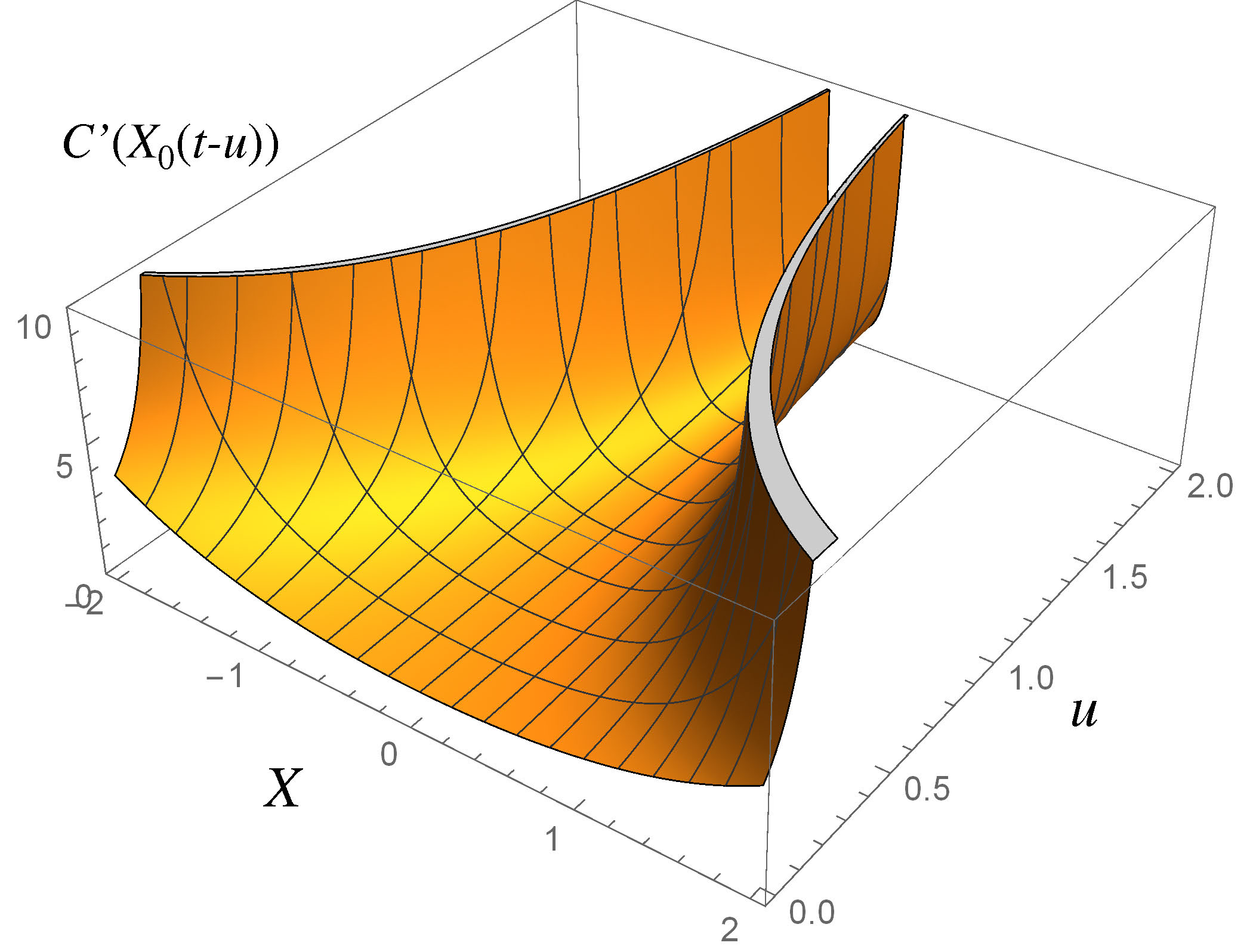
Figure 7: $C^{\prime}(X)$ along the backward evolution $X_{0}(X;-u)$, $X_{0}(X;0)=X$, for the hyperbolic drift fields $C(X)=\alpha\sinh(kX)$, $\alpha=k=1$.

Figure 8: $C^{\prime}(X)$ along the backward evolution $X_{0}(X;-u)$, $X_{0}(X;0)=X$, for the pure cubic drift fields $C(X)=\alpha X^{3}$,$\alpha=1$.

Figure 9: $C^{\prime}(X)$ along the backward evolution $X_{0}(X;-u)$, $X_{0}(X;0)=X$, for the drift fields $C(X)=X+\alpha X^{3}$,$\alpha=1$. For $|X|<1$ $C^{\prime}(X_{0}(X;-u))$ decreases with $u$ (the inset is a magnification of the interval $|X|<1$), while for $|X|>1$ it increases.

We would like to add a few comments about the divergence of the backward evolution $X_{0}(X;-u)$: we have seen that there are drift fields such that for any initial position $X_{0}(X;0)=X$, the backward evolution diverges with an asymptote at a given finite time $\bar{u}(X)=\int_{X}^{\infty}\frac{1}{c(y)}\;dy$. This behaviour is shown in Figs. 7, 8 and 9 for three different drift fields, respectively: in the first two cases we observe a divergency for any initial $X$ (that means a finite $\bar{u}(X)$ value), in the last case there is clearly a range of $X$ where the backward evolution does not diverge (thus, $\bar{u}(X)=\infty$). On the other hand, the important case of Brownian motion in a periodic potential, a heuristic model with applications in various branches of science and technology, like the diffusive dynamics of atoms and molecules on crystal surfaces Ala-Nissila et al. (2002), modelled using $C(X)=\alpha\sin(kX)$, is such that $\bar{u}(X)=\infty$ $\forall X$. In fact, the function $C(X)/C(X_{0}(X;-u))$ is always positive and simply increases with $u$ as $e^{k\alpha u}$. Therefore in this case the “standard” BFPE formula of Eq. (19) for the diffusion coefficient is correct.

IV A comparison with the Local Linearization Approach

As we mentioned in the Introduction, very often the LLA FPE turns out to be fairly close to the numerical simulations. This is shown in Fig. 10, for the case $C(X)=\alpha\sinh(kX)$. We are going to show that this is not a coincidence: as a matter of fact, the LLA FPE is an excellent approximation of the cBFPE, when the latter is applicable (i.e., typically, small $\epsilon$ and finite, but not small, $\tau$).

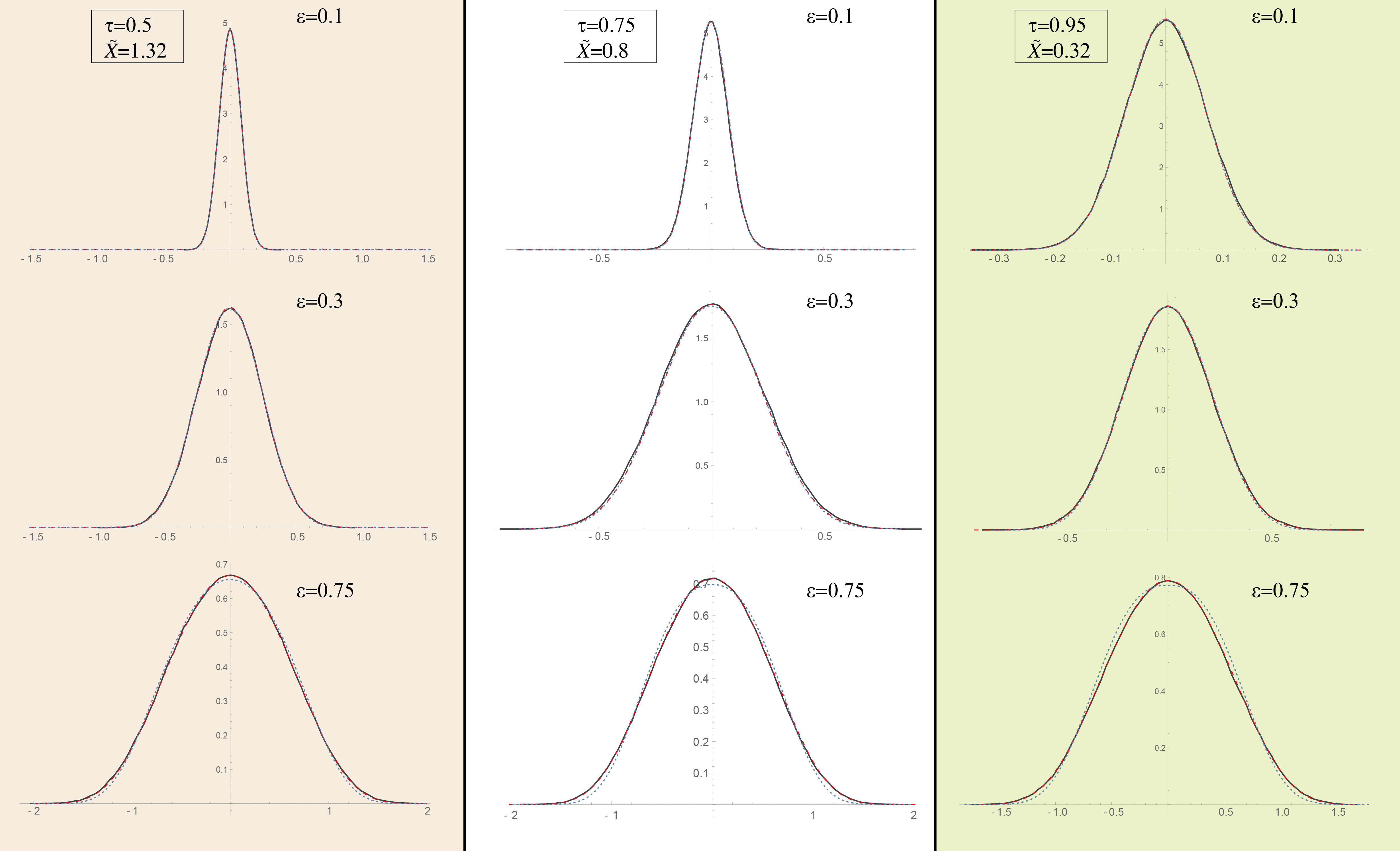
Figure 10: The same as Fig. 2 but without the $P_{s}(X)_{BFPE}$ and with inserted the $P_{s}(X)_{LLA}$. Namely, solid black lines: the stationary PDF from the numerical simulations of the SDE of Eq. (1) with $C(X)=\sinh(X)$. Dotted blue lines: the cBFPE stationary PDF $P_{s}(X)_{cBFPE}$ obtained from Eq. (5) using $D(X)=D(X,\infty)_{cBFPE}$ of Eq. (III). Dashed red lines (barely visible close or under the solid lines): $P_{s}(X)_{LLA}$ of Eq. (IV). The three columns correspond to three different values for $\tau$, while the three rows corresponds to three different values for $\epsilon$. Note the excellent agreement between simulations and LLA PDF.

We need to briefly go through the derivation of the LLA FPE. West at al. have shown Peacock-López et al. (1988) that the LLA FPE can be formally derived from the BFPE of Eq. (II) as follows:

1. there is a large enough time-scale separation between the unperturbed dynamics and the decay time of the correlation function $\varphi(t)$, so that the unperturbed dynamics $X_{0}(X;-u)$ can be considered close to the initial position $X$;

2. assuming a above, rather than expanding $\frac{1}{C(X_{0}(X;-u))}$ in powers of $u$ (which would give rise to the same secular terms as the expansion in Eq. (II)), expand its logarithm

   $$\frac{1}{C(X_{0}(X;-u))}=e^{\log\left(\frac{1}{C(X_{0}(X;-u))}\right)}$$

   $$=e^{\log\left(\frac{1}{C(X)}\right)-C^{\prime}(X)\,u-\frac{1}{2}C(X)C^{\prime\prime}(X)\,u^{2}+O(u^{3})},$$ (26)

   and truncate the series at the first order.

Using point b in Eq. (II), we are led to the LLA FPE (here generalized to finite times and to a generic correlation function of the noise):

$$\partial_{t}{P}(X;t)\sim{\cal L}_{a}P(X;t)$$

$$+\epsilon^{2}\frac{1}{\tau}\partial_{X}^{2}\left(\int_{0}^{t}\mbox{d}u\,e^{-C^{\prime}(X)u}\varphi(u)\right){P}(X;t).$$ (27)

Note that for $C(X)=\gamma X$, the series expansion of the r.h.s. of Eq. (b) stops exactly at the first order in $u$, while this does not happen expanding the term $1/C(X_{0}(X;-u))$. Therefore, instead of using the West and al. approach (given by a-b above) to go from the BFPE to the LLA FPE, the latter can be directly obtained by replacing the function $C(X)/C(X_{0}(X;-u))$ with an exponential function with state dependent decay coefficient $C^{\prime}(X)$: $C(X)/C(X_{0}(X;-u))\to\exp(-C^{\prime}(X)u)$). From Eq. (IV) we get the following result for the state dependent diffusion coefficient of the FPE:

$$D(X,t)_{LLA}=\epsilon^{2}\frac{1}{\tau}\,\left(\int_{0}^{t}\mbox{d}u\,e^{-C^{\prime}(X)u}\varphi(u)\right)$$ (28)

that, for large times becomes

$$D(X,\infty)_{LLA}=\epsilon^{2}\,\frac{\hat{\varphi}(C^{\prime}(X))}{\tau}$$ (29)

where $\hat{\varphi}$ stands for Laplace transform of $\varphi$. From Eq. (28) it turns out that $D(X,\infty)_{LLA}$ exists and is positive under fairly general conditions. For example, considering again the case $C(X)=\alpha\sinh(kX)$, from Eq. (28) we easily get

$$D(X,\infty)_{LLA}=\frac{\epsilon^{2}}{1+\alpha k\tau\cosh(kX)},$$ (30)

where the only constraint is that the flow is not divergent (namely, $\alpha>0$). Using Eq. (30) in Eq. (5) we obtain the LLA stationary PDF for this case:

$$P_{s}(X)_{LLA}$$

$$=\frac{1}{Z_{LLA}}\left(\frac{1+\alpha k\tau\cosh(kX)}{1+\alpha k\tau}\right)e^{-\frac{\alpha\sinh^{2}\left(\frac{kX}{2}\right)(\alpha k\tau+\alpha k\tau\cosh(kX)+2)}{k\epsilon^{2}}},$$ (31)

In Appendix A we report the LLA results for the cubic case. In Fig. 10 we can see the stationary PDFs of the LLA FPE, together with the results from the cBFPE: the agreement with the numerical integration of the SDE of Eq. (1) is very good.

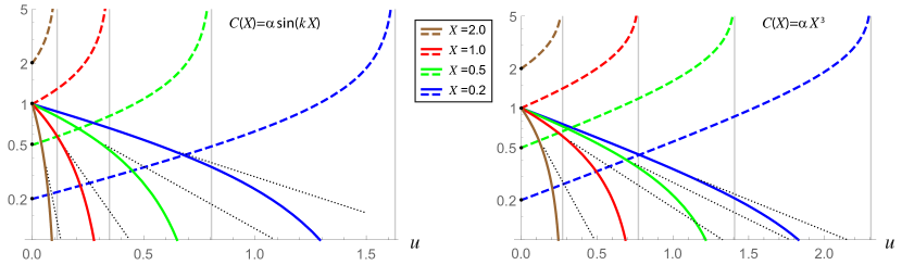
Figure 11: Left (right), the same of Fig. 3 (Fig. 4) but in log scale. The dotted black lines correspond to the LLA approximation. We can see that the deviation from the exponential decay of the function $C(X)/C(X_{0}(X;-u))$ (solid lines) is relevant only in the final part, where the value of the function is relatively small.

Fig. 11 compares the kernels of the cBFPE and of the LLA for the cases $C(X)=\alpha\sinh(kX)$ and $C(X)=\alpha X^{3}$. It turns out that the LLA kernel (dotted lines) is an excellent approximation of the cBFPE kernel. It is hence not surprising that the LLA PDF is as close to the simulations as it is the cBFPE PDF.

This is a nice explanation of what has been down heuristically in the literature: the LLA approach of Grigolini Tsironis and Grigolini (1988a); Faetti et al. (1988) is indeed based on the assumption that, for any value of $X$, we can safely replace the unperturbed backward evolution of the function $f(X,u):=C(X)/C(X_{0}(X;-u))$, with an exponential function of the time $u$, with the $X$ dependent exponent: $f(X,u)\sim\exp[-C^{\prime}(X)u]$. For one-dimensional dissipative systems, the exponential behavior of such a back time evolution is typical.

Actually, there is another general argument, not related to the cBFPE, that leads us to speculate that typically (but not always), the LLA FPE works well, also for strong perturbations. In fact it is possible to prove that the LLA and the Fox functional-calculus Fox (1986b, a) corresponds to the Almost Gaussian Assumption for generalized stochastic operators Bianucci (2018): independently of the value of $\epsilon$, when $\xi(t)$ is a Gaussian stochastic process, the LLA typically makes almost vanishing all the terms, appearing in the projection/cumulant expansion, which would destroy the FPE. This means that often the LLA FPE would be valid even for large $\epsilon$ values for which the cBFPE breaks down (but a counterexample is shown if Fig. 13).

On the other hand, if the stochastic process $\xi(t)$ is not Gaussian, or it is not at all stochastic (for example, it is the degree of freedom of a chaotic dynamical system), then the Almost Gaussian Assumption or the Fox functional calculus can no longer be advocated to give an a priori justification (although weak) to the LLA FPE. In these cases, a small $\epsilon$ value and the cBFPE would be the only possible approach for a proper FPE treatment, and the LLA FPE could be, at the best, an approximation of the cBFPE.

V Conclusions

By definition, the BFPE is the best FPE we can get from a perturbation approach starting from a SDE. In this work we are interested in the 1-d case with additive noise as in Eq. (1), in which $\epsilon$ is the small parameter. For the 1-d case the BFPE was obtained many years ago by Lopez, West and Lindenberg Peacock-López et al. (1988), but their result reveals unphysical features. In particular, if $\tau$ and $\epsilon$ are not fairly small, it may lead to negative values both of the diffusion coefficient and of the PDF, in some region of the state space. It is customary to cure this situation by simply restricting the domain of support of the PDF to exclude these regions. It has been argued that this unphysical result of the BFPE might point to problems in the model used to represent the physical system Peacock-López et al. (1989). In this work we show, on the contrary, that these problems are due to an incorrect use of the perturbation approach for dissipative systems. In particular, a proper use of the interaction picture fixes the problem. The cBFPE gives results that are close to those of numerical simulations of the SDE of Eq. (1), even for values of $\epsilon$ and $\tau$ well beyond those allowed by the classical BFPE. The stationary PDF is now similar also to that obtained from the LLA FPE of Grigolini Tsironis and Grigolini (1988a); Faetti et al. (1988) and Fox Fox (1986a).

Appendix A The cubic case

We briefly present the results for the pure cubic case, namely $C(X)=X^{3}$. This is an extreme non linear case, in fact, also small oscillations are non-linear. It is no coincidence that the standard BFPE cannot be used in this case (see below).

From Eq. (19) we easily obtain,

$$D(X,t)_{BFPE}= \epsilon^{2}\,\frac{1}{2}\,e^{-\frac{t}{\tau}}\bigg{[}(2\sqrt{1-2tX^{2}}e^{\frac{1}{2\tau X^{2}}}\left(2tX^{2}+3\tau X^{2}-1\right)$$

$$\left.-3\sqrt{2\pi}\tau^{3/2}X^{3}e^{t/\tau}\,\text{erfi}\left(\frac{\sqrt{\frac{1}{2}-tX^{2}}}{\sqrt{\tau}X}\right)\right]e^{-\frac{1}{2\tau X^{2}}}$$

$$-\frac{1}{2}\tau\left[-3\sqrt{2\pi}\tau^{3/2}X^{3}e^{-\frac{1}{2\tau X^{2}}}\,\text{erfi}\left(\frac{1}{\sqrt{2}\sqrt{\tau}X}\right)+6\tau X^{2}-2\right]$$ (32)

that, for $t>2X^{2}$ is a complex number: for large times it is not defined. This means that for a cubic drift field, by using the standard BFPE a stationary PDF cannot be obtained. The situation is different exploiting our correction to the BFPE. In fact, for large times ($t\to\infty$), we have (see Eq. (III)

$$D(X,\infty)_{cBFPE}=D(X,\bar{u}(X))_{BFPE}$$

$$=\epsilon^{2}\,\left[1+3\tau X^{2}\left(\sqrt{2}\sqrt{\tau}XF\left(\frac{1}{\sqrt{2}X\sqrt{\tau}}\right)-1\right)\right]$$ (33)

where $F(x):=e^{-x^{2}}\int_{0}^{x}e^{y^{2}}\,\text{d}y=e^{-x^{2}}\frac{\sqrt{\pi}}{2}\text{erfi}(x)$ is the Dawson function. The diffusion coefficient of Eq. (A) is now positive and well defined for any $X$. Concerning the LLA diffusion coefficient, from Eq. (29) we easily get:

$$D(X,\infty)_{LLA}=\frac{\epsilon^{2}}{3\tau X^{2}+1}.$$ (34)

In Fig. (12) we compare the corrected BFPE and the LLA diffusion coefficients, respectively. Inserting in Eq. (5) the expressions in Eqs. (A))-(34)), we obtain the stationary PDF shown in Fig. 13. We see that in this extreme non linear case, where the standard BFPE cannot be used, our corrected BFPE gives results that, for small $\epsilon$, are in agreement with numerical simulations of the SDE. Notice that, in this case, also the LLA fails for large $\epsilon$ values.

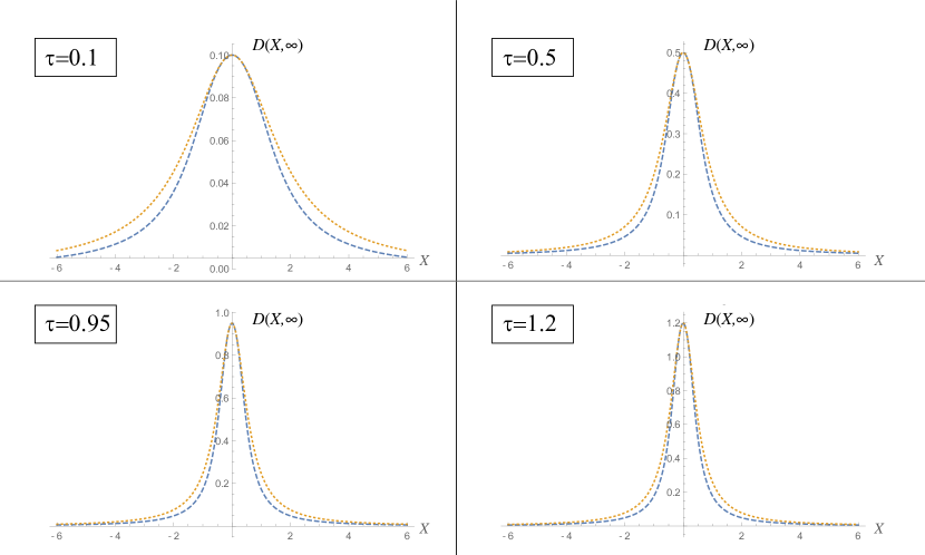
Figure 12: Diffusion coefficients for a pure cubic drift field. The BFPE gives an imaginary result, thus in this case cannot be used. Dashed blue lines: the $D(X,\infty)_{cBFPE}$ of Eq. (A) for different values of $\tau$. Dotted orange line: the $D(X,\infty)_{LLA}$ of Eq. (34) for the same values of $\tau$.

4

Figure 13: The stationary PDF for the SDE of Eq. (1) where $C(X)=X^{3}$ and $\xi(t)$ is a Gaussian noise with correlation function $\varphi(t)=\exp(-t/\tau)$. In this case the standard BFPE cannot be used because it leads to an imaginary diffusion coefficient $D(X,\infty)_{BFPE}$ (see text). The four columns correspond to four different values for $\tau$, while the four rows corresponds to four different values for $\epsilon$. Solid black lines: the results of the numerical simulation of the SDE. Dashed blue lines: the corrected BFPE results, namely the PDF of Eq. (5) where the diffusion coefficient is given in Eq. (A). Dotted orange lines: the LLA result, namely the PDF of Eq. (5) where the diffusion coefficient is given in Eq. (34).

References

- Schadschneider et al. (2010) A. Schadschneider, D. Chowdhury, and K. Nishinari, eds., Stochastic Transport in Complex Systems. From Molecules to Vehicles (Elsevier, Amsterdam, 2010).
- Peacock-López et al. (1988) E. Peacock-López, B. J. West, and K. Lindenberg, Phys. Rev. A 37, 3530 (1988).
- Tsironis and Grigolini (1988a) G. P. Tsironis and P. Grigolini, Phys. Rev. A 38, 3749 (1988a).
- Fox (1986a) R. F. Fox, Phys. Rev. A 34, 4525 (1986a).
- Zhu et al. (1986) S. Zhu, A. W. Yu, and R. Roy, Phys. Rev. A 34, 4333 (1986).
- Zhu (1993) S. Zhu, Phys. Rev. A 47, 2405 (1993).
- Da-jin et al. (1989) W. Da-jin, C. Li, and Y. Bo, Communications in Theoretical Physics 11, 379 (1989).
- Dong-cheng et al. (1999) M. Dong-cheng, X. Guang-zhong, C. Li, and W. Da-jin, Acta Physica Sinica (Overseas Edition) 8, 174 (1999).
- Oliveira (1998) F. Oliveira, Physica A: Statistical Mechanics and its Applications 257, 128 (1998).
- Fonseca et al. (1985) T. Fonseca, P. Grigolini, and D. Pareo, The Journal of Chemical Physics 83, 1039 (1985).
- Bianucci and Grigolini (1992) M. Bianucci and P. Grigolini, The Journal of Chemical Physics 96, 6138 (1992).
- Bianucci et al. (1990) M. Bianucci, P. Grigolini, and V. Palleschi, The Journal of Chemical Physics 92, 3427 (1990).
- Lebreuilly et al. (2016) J. Lebreuilly, M. Wouters, and I. Carusotto, Comptes Rendus Physique 17, 836 (2016), polariton physics / Physique des polaritons.
- Horsthemke and Lefever (1984) W. Horsthemke and R. Lefever, Noise-Induced Transitions. Theory and Applications in Physics, Chemistry, and Biology, 1st ed., Springer Series in Synergetics, Vol. 15 (Springer-Verlag Berlin Heidelberg, 1984) pp. XVI, 322.
- Jin et al. (2007) F.-F. Jin, L. Lin, A. Timmermann, and J. Zhao, Geophysical Research Letters 34, L03807 (2007), l03807.
- Bianucci (2016) M. Bianucci, Geophysical Research Letters 43, 386 (2016), 2015GL066772.
- Note (1) The general prescription is that there is a time such that, for any time , the instances of at times are “almost statistically uncorrelated” with the instances of at times . For “almost statistically uncorrelated” we mean that the joint probability density functions factorizes up to terms : with , and . For example, .
- Adelman (1976) S. A. Adelman, The Journal of Chemical Physics 64, 124 (1976).
- Kubo (1962) R. Kubo, Journal of the Physical Society of Japan 17, 1100 (1962), https://doi.org/10.1143/JPSJ.17.1100 .
- Kubo (1963) R. Kubo, Journal of Mathematical Physics 4, 174 (1963), https://doi.org/10.1063/1.1703941 .
- Bianucci (2018) M. Bianucci, Journal of Mathematical Physics 59, 053303 (2018), https://doi.org/10.1063/1.5037656 .
- Fox (1986b) R. F. Fox, Phys. Rev. A 33, 467 (1986b).
- Grigolini and Marchesoni (1985) P. Grigolini and F. Marchesoni, in Memory Function Approaches to Stochastich Problems in Condensed Matter, Advances in Chemical Physics, Vol. LXII, edited by M. W. Evans, P. Grigolini, and G. P. Parravicini (An Interscience Publication, John Wiley & Sons, New York, 1985) Chap. II, p. 556.
- Grigolini (1989) P. Grigolini, in Noise in Nonlinear Dynamical Systems, Vol. 1, edited by F. Moss and P. V. E. McClintock (Cambridge University Press, Cambridge, England, 1989) Chap. 5, p. 161.
- Bianucci (2015) M. Bianucci, Journal of Statistical Mechanics: Theory and Experiment 2015, P05016 (2015).
- Note (2) Actually, the derivation shown here is a generalization, since we do not assume that and we do not take the limit in the time integration.
- Lindenberg and West (1983) K. Lindenberg and B. J. West, Physica A: Statistical Mechanics and its Applications 119, 485 (1983).
- Masoliver et al. (1987) J. Masoliver, B. J. West, and K. Lindenberg, Phys. Rev. A 35, 3086 (1987).
- Tsironis and Grigolini (1988b) G. P. Tsironis and P. Grigolini, Phys. Rev. Lett. 61, 7 (1988b).
- Grigolini et al. (1988) P. Grigolini, L. A. Lugiato, R. Mannella, P. V. E. McClintock, M. Merri, and M. Pernigo, Phys. Rev. A 38, 1966 (1988).
- Ala-Nissila et al. (2002) T. Ala-Nissila, R. Ferrando, and S. C. Ying, Advances in Physics 51, 949 (2002).
- Faetti et al. (1988) S. Faetti, L. Fronzoni, P. Grigolini, and R. Mannella, Journal of Statistical Physics 52, 951 (1988).
- Peacock-López et al. (1989) E. Peacock-López, F. J. de la Rubia, B. J. West, and K. Lindenberg, Physics Letters A 136, 96 (1989).