Probabilistic 3D Multilabel Real-time Mapping
for Multi-object Manipulation

Abstract

Probabilistic 3D map has been applied to object segmentation with multiple camera viewpoints, however, conventional methods lack of real-time efficiency and functionality of multilabel object mapping. In this paper, we propose a method to generate three-dimensional map with multilabel occupancy in real-time. Extending our previous work [1] in which only target label occupancy is mapped, we achieve multilabel object segmentation in a single looking around action. We evaluate our method by testing segmentation accuracy with 39 different objects, and applying it to a manipulation task of multiple objects in the experiments. Our mapping-based method outperforms the conventional projection-based method by 40 - 96% relative (12.6 mean $IU_{3d}$), and robot successfuly recognizes (86.9%) and manipulates multiple objects (60.7%) in an environment with heavy occlusions.

I Introduction

Probabilistic three-dimensional map has been applied to navigation and manipulation in previous works [2, 3], however, the generated map has only the collision information, and is not applicable to multi-object manipulation because of lacking label information of objects.

Recently, the effectiveness of probabilistic map for object segmentation is reported [4], which uses the map to improve 2D segmentation result. However, their research lacks of consideration of real-time efficiency, which is crucial for 3D segmentation of objects and its manipulation. On the other hand, we have proposed real-time 3D mapping for a single label object [1]. In order for robot to conduct tasks that demands multi-object segmentation at once; for example multi-object manipulation (Fig.1), we propose a method to construct three-dimensional map for multi-label objects in real-time.

The proposed method extends our previous method for a single label of objects [1], and represents object-label and collision with multilabel occupancies in each voxel. For real-time map generation, we extend octomap [3] for multi-label objects, which is firstly proposed to efficiently map single-label, collision object, occupancy. By accumulating the 2.5D segmentation results in possible camera viewpoints, our method segments multiple objects three-dimensionally all at once (Fig.1). We show the efficiency of our method compared to non-mapping-based method and a multi-object manipulation task in the experiment.

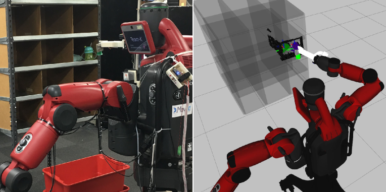
(a) Manipulating objects with result of 3D segmentation.

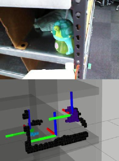
(b) View 1

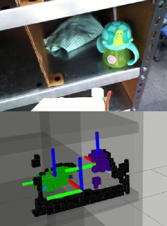
(c) View $\sim$ 3

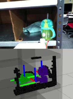
(d) View $\sim$ 5

Figure 1: Real-time mapping for multi-object manipulation. In this example, target object (t-shirts) is occluded by non-target (green cup), and robot needs to remove the obstacle object in order to pick the target with recognizing the necessity of doing so.

II 3D Multilabel Mapping for
Object Segmentation and Manipulation

II-A Related Works

II-A1 Object Segmentation

In previous works, 2D object segmentation is tackled as a contour finding problem with a guide of region-of-interest [5][6], a superpixel classification [7][8] and pixel-wise classification [9][10][11] with learning-based approach with class segmentation dataset. In addition to these works on 2D segmentation, three-dimentional segmentation is required for robot to conduct tasks in the real world. In order to achieve this, previous works propose projection-based approach projecting segmented pixels to 3D points in a single view (2.5D) [9], mapping-based approach with binary object existence [12] and probabilistic existence [1] for a single target object. And as for fully 3D-based approach, model matching is tackled [13][14] using various 3D features [15][16]. We use a mapping-based approach with multiple views extending our previous method [1] for multi-label objects to deal with object occlusions and flexible objects for which static 3D model is less effective. Our method segments multi-label objects in a single multi-view action, and effective to acquire the dense 3D information of objects in an environment with heavy occlusions: self-occlusion and occlusion by others.

II-A2 Probabilistic Grid Map

In previous works on probabilistic grid map, object exploration with updating object existence probability on 2D map [17], collision object [3][18] and object segmentation on 3D map [4][1] are tackled. Our proposed method is most closely related to two prior works [4][1], and the contribution of this paper is the proposed octomap that has a single octree with multilabel probabilities in the nodes. Compared to the previous methods to update a single-label occupancy, our method updates the multilabel occupancies in each voxel, and segments all objects in a single mapping.

II-A3 Multi-object Manipulation

We define multi-object manipulation as a task to handle multiple objects with determination of the order to manipulate. Its typical situation is a picking task with occluded target object, where robot needs to recognize both the target and occluding objects in order to remove firstly the occluding and pick the target later. In previous works, multi-object manipulation is tackled in simulation [19], and in a simple real world environment with single-class objects [20][21], We address manipulation task of multi-class multiple objects in a clutter environment that contains heavy occlusions.

II-B Proposed Method and System

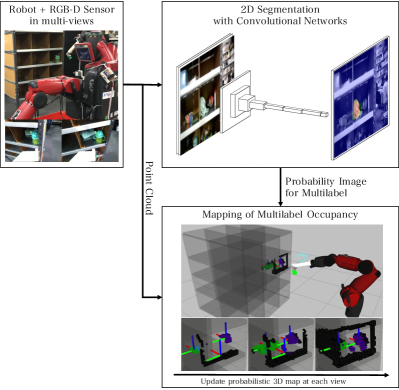
Figure 2: Proposed system for 3D object segmentation.

In this paper, we propose a probabilistic mapping method for multilabel occupancies, in which each voxel grid has probabilities for all object labels ($n_{label}\sim 40$ in the experiment). In a voxel, each label occupancy is updated separately and the maximum occupancy is used to transform the map to voxels: if the maximum occupancy is over a threshold, it is occupied by the label and otherwise unoccupied.

We also propose a 3D segmentation system shown in Fig.2, which is extended version of system in prior work [1] for multilabel segmentation. Our system consists of 2 components: 2D segmentation and 3D mapping. In the first component, 2D object probability image $I^{prob}_{t}$ is predicted at time $t$ from input image $I_{t}$, and the output probability image $I^{prob}_{t}$ has same number of channels as the number of object classes $n_{label}$. In the second component, our 3D mapping method for multilabel $M_{t}=g(M_{t-1},I^{prob}_{t},C_{t})$ is used to update the grid map $M_{t-1}$ with input point cloud $C_{t}$, after projecting the pixel to 3D point with index of height and width axies $u,v$,

$$z_{t,uv}=(C_{t,uv},I^{prob}_{t,uv})$$ (1)

with correspondence between image and point cloud: assuming that the point cloud comes from RGB-D camera sensor. By accumulating the object probability prediction result three-dimensionally as a map, we improve 3D object segmentation result in a situation with occlusions and generate dense 3D object voxel map.

In the following sections, we introduce the method to predict object probability from input image in Section III, and the method of 3D mapping in Section IV. In Section V, we evaluate the efficiency of our proposed method with quantitative evaluation of the segmentation and achievement of multi-object manipulation by a robot.

III Probabilistic Object Segmentation
in a Single View

In this section, we introduce the function $(C_{t,uv},I^{prob}_{t,uv})=f(I_{t})$ which receives RGB image $I_{t}$ as the input and outputs multi-class probabilities $I_{t,uv}^{prob}$ and 3D point $C_{t,uv}$ at pixel $(u,v)$ as the output. We briefly describe the network model for this function because it is same as that developed in our previous work [1], and discuss about the efficiency by using 2D segmentation as a component in the 3D segmentation system.

III-A Convolutional Network Model

We use a previously proposed convolutional network model for 2D segmentation, Fully Convolutional Networks (FCN) [10], applying a small change to convert n-class object score map $I^{score}$, the output of the network, to probability image $I^{prob}$ using pixel-wise softmax with index for height $u\in[0,H]$, width $v\in[0,W]$ and channel $k\in[0,n_{label}-1]$ for image height $H$ and width $W$:

$$I^{prob}_{uv}=\sigma(I^{score}_{uv})=\frac{exp(I^{score}_{uv})}{\sum^{N}_{k=0}exp(I^{score}_{uvk})}.$$ (2)

III-B Projection of 2D segmentation as 3D points

For 3D mapping, the pixel-wise 2D segmentation needs to be projected to 3D points. By using a calibrated camera, we can project the pixel point in 2D segmentation to the 3D point:

$$\begin{bmatrix}u\\ v\\ Z_{c}\end{bmatrix}=K\begin{bmatrix}X_{c}\\ Y_{c}\\ Z_{c}\end{bmatrix},K=\begin{bmatrix}f_{x}&0&c_{x}\\ 0&f_{y}&c_{y}\\ 0&0&1\end{bmatrix}.$$ (3)

$(X_{c},Y_{c},Z_{c})$ are the coordinates of a 3D point in the camera coordinate space, $(u,v)$ are the coordinates of a projection point in camera pixels, and $K$ is the matrix of camera intrinsic parameters.

Using RGB-D camera, whose extrinsic parameters between color and depth sensor coordinate are well calibrated, the pixelwise depth $d$ in color coordinate is given, and the 3D point coodinates are given as follows:

$$X_{c}=\frac{u-c_{x}Z_{c}}{f_{x}},Y_{c}=\frac{v-c_{y}Z_{c}}{f_{y}},Z_{c}=d.$$ (4)

Therefore, 3D point in world coordinate space is given with a homogeneous transformation matrix $A$ from camera to world coodinate:

$$\begin{bmatrix}X\\ Y\\ Z\\ 1\end{bmatrix}=A\begin{bmatrix}X_{c}\\ Y_{c}\\ Z_{c}\\ 1\end{bmatrix},A=\begin{bmatrix}r_{11}&r_{12}&r_{13}&t_{1}\\ r_{21}&r_{22}&r_{23}&t_{2}\\ r_{31}&r_{32}&r_{33}&t_{3}\\ 0&0&0&1\end{bmatrix}$$ (5)

In the experiment, since the RGB-D sensor is mounted on the robotic arm and the task is conducted without navigation, we use the transformation matrix $A$ computed from joint angles of the arm and forward kinematics.

In the 3D mapping we describe at afterward sections, the set of multi-class probabilities $I^{prob}_{uv}$, and 3D point $C_{t,uv}=(X,Y,Z)$ is used to accumulate the pixel-wise 2D segmentation into 3D map.

IV 3D Mapping of Multilabel Occupancy

In this section, we introduce the function $M_{t}=g(M_{t-1},I_{t,uv}^{prob},C_{t,uv})$ to generate voxel grid map $M_{t}$ from 2D probability map $I_{t}^{prob}$ and input point cloud $C_{t,uv}$. We describe the method to contruct voxel map for multilabel occupancy, and to update the map in real-time.

IV-A Generating Occupancy Map for Multilabel

In conventional occupancy grid map [18], the $l$-th cell $m_{s}$ holds the probability of occupancy for collision object $p^{collision}(m_{s})$. In our occupancy voxel map, on the other hand, each grid has the same number of probabilities as the number of labels $n_{label}$. Each probability has the value between 0 and 1:

$$0\leq p_{k}(m_{s})\leq 1\quad(k=0\cdots n_{label}-1)$$

and meaning of the value is represented as following:

$$\begin{cases}m_{s}:unoccupied&(\max_{k}(p_{k}(m_{s}))<p_{thresh})\\ m_{s}:occupied~{}by~{}l_{s}&(\max_{k}(p_{k}(m_{s}))>=p_{thresh})\\ \end{cases}$$ (6)

with occupied label $l_{s}=\operatornamewithlimits{argmax}_{k}(p_{k}(m_{s}))$. The occupancy threshold $p_{thresh}$ is set to $0.5$ in our experiments.

We explain the method of updating $p_{k}(m_{s})$ from sensor information $z_{t}$; $t$ is the index in series of sensor input, $z_{t}$ is the set of sensor information at the time index $t$, and $z_{1:t}$ means the set of the sensor information from first to the $t$-th time. Notice that $z_{t,uv}$ (Equation 1) is set of the point cloud $C_{t}$ and 2D probability image $I_{t}^{prob}$, and the probability in each pixel $I_{t,uv}^{prob}$ is registered to a 3D point $C_{t}=(X,Y,Z)$ by Equation 3 - 5.

By computing $p_{k}(m_{s}|z_{1:t})$ with $p_{k}(m_{s}|z_{1:t-1})$ and $z_{t}$, we can integrate new sensor information and update the map periodically. The grid map $M_{t}$ is the set of voxels with multilabel probabilities accumulated in them $p_{k}(m_{s}|z_{1:t})$: $m_{s}$ is one of the voxels whose size is $S$: $s=0\cdots S$. Using each 3D point $z_{t,uv}=(C_{uv},I^{prob}_{uv})$, occupancies in multiple voxels are updated, because the sensed 3D point $C_{uv}$ has two parts of information: the voxel at $C_{uv}$ has collision object (hit), the voxels on the ray from camera coordinate to $C_{uv}$ has no collision objects (miss). Using these information, the new probability $p_{k}(m_{s}|z_{t})$ is acquired as following with $m_{s}$ is given by $C_{t,uv}$:

$$\begin{cases}p_{k}(m_{s}|z_{t})=I_{t,uvk}^{prob}&(m_{s}:hit)\\ p_{k}(m_{s}|z_{t})=p_{miss}&(m_{s}:miss)\\ \end{cases}$$ (7)

In the following experiments, we used $p_{miss}=0.3$, which is the probability for the voxel where the point cloud is missing.

Next we need to compute $p_{k}(m_{s}|z_{1:t})$ from $p_{k}(m_{s}|z_{1:t-1})$ and $p_{k}(m_{s}|z_{t})$. Following formula is derived from Bayes’ theorem and independence of the conditional probability:

$$p_{k}(m_{s}|z_{1:t}) = \frac{p_{k}(z_{t}|m_{s},z_{1:t-1})\ p_{k}(m_{s}|z_{1:t-1})}{p_{k}(z_{t}|z_{1:t-1})}$$ (8)

$$= \frac{p_{k}(m_{s}|z_{t})\ p_{k}(z_{t})\ p_{k}(m_{s}|z_{1:t-1})}{p_{k}(m_{s})\ p_{k}(z_{t}|z_{1:t-1})}.$$

The ratio of occupied probability $p_{k}(m_{s}|z_{1:t})$ and free probability $p_{k}(\lnot m_{s}|z_{1:t})$ becomes simple as following:

$$\frac{p_{k}(m_{s}|z_{1:t})}{p_{k}(\lnot m_{s}|z_{1:t})}=\frac{p_{k}(m_{s}|z_{1:t-1})}{p_{k}(\lnot m_{s}|z_{1:t-1})}\frac{p_{k}(m_{s}|z_{t})}{p_{k}(\lnot m_{s}|z_{t})}\frac{p_{k}(\lnot m_{s})}{p(m_{s})}.$$ (9)

We can deform the formula by introducing log-odds (logit) as following:

$${\cal L}(m_{s}|z_{1:t})={\cal L}(m_{s}|z_{1:t-1})+{\cal L}(m_{s}|z_{t})-{\cal L}(m_{s}).$$ (10)

$${\rm where}\ \ \ \ {\cal L}(x)={\rm logit}(p(x))=\log(p(x)/(1-p(x)))$$

Presuming that we have no prior knowledge of the environment at the first time ($t=0$): ${\cal L}(m_{s})=0~{}(\because p(m_{s})=0.5)$, therefore ${\cal L}(m_{s}|z_{1:t})$ is updated as following:

$${\cal L}(m_{s}|z_{1:t})={\cal L}(m_{s}|z_{1:t-1})+{\cal L}(m_{s}|z_{t}).$$ (11)

We can update the map probabilistically using this formula, and obtain probability $p_{k}(m_{s}|z_{1:t})$ from the log-odds ${\cal L}(m_{s}|z_{1:t})$ as following:

$$p_{k}(m_{s}|z_{1:t})=1-(1+\exp({\cal L}(m_{s}|z_{1:t})))^{-1}.$$ (12)

IV-B Extending OctoMap for Multilabel Occupancy

For real-time updation of the map, we extend the OctoMap [3], which is an efficient framework to generate occupancy grid map using octree. In the octomap with multilabel occupancy (LabelOctoMap), which we propose, each node in octree has multiple probabilities and the number of nodes is same as that of voxels $S$, which depends on the resolution of voxels not the number of labels. So the search of the voxel to be updated from 3D coordinate in LabelOctoMap is as efficient about speed as the conventional octomap.

Having a single tree is also effective for reconstruction of voxels from the map compared to the use of multiple octrees for multi-labels. As shown in Equation 6, we find label with maximum likelihood for each voxel, and this operation is required because it is possible that probabilities of multiple labels can be over threshold $p_{threshold}$ for voxels at the same 3D coordinate. The comparison of probabilities is time consuming when using multiple octrees, because each comparison requires the search of the corresponding voxel in a tree from 3D coordinate of the voxel in other tree.

V Experiments

In this section, we show the evaluation result of our proposed method with the segmentation accuracy tests and the robotic manipulation task application.

V-A Evaluate 2D Segmentation

We describe the evaluation results of the trained model, in order to show the effectiveness of using 2D segmentation as a component of the system, though there are previous works which use fully 3D approach [13][14]. We use the validation dataset ($\sim 1900$) with splitting the whole dataset in 4:1 for training and validation.

V-A1 Dataset and training

We handle 39 objects (Fig.3), which were used at Amazon Picking Challenge 2016 (APC2016), in an environment shown in Fig.1. So the number of object classes is 40: 39 item labels and 1 background label. The number written in Fig.3 is each item’s label and 0 is the background label. For dataset, we combined the dataset we previously collected [1] ($\sim 250$) and that is published by other work [12] ($\sim 7300$).

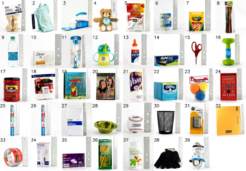
Figure 3: 39 objects used at APC2016.

V-A2 Evaluation Metric

The metric of quantitative evaluation is same as one used in previous work [10]:

• pixel accuracy: $\sum_{i}n_{ii}/\sum_{i}t_{i}$

• mean accuracy: $(1/n_{label})\sum_{i}n_{ii}/t_{i}$

• mean intersect-over-union (IU):
  $(1/n_{label})\sum_{i}n_{ii}/(t_{i}+\sum_{j}n_{ji}-n_{ii})$

• frequency weighted IU:
  $(\sum_{k}t_{k})^{-1}\sum_{i}t_{i}n_{ii}/(t_{i}+\sum_{j}n_{ji}-n_{ii})$

where $n_{ij}$ is the number of pixels of class $i$ predicted to belong to class $j$, $n_{label}$ the number of classes, and $t_{i}=\sum_{j}n_{ij}$ is the total number of pixels of class $i$. All metrics have value range $[0,1]$ so we values multiplied by 100.

V-A3 Result

The quantitative result of the FCN model with different datasets (Table I) shows that the model trained with our dataset is as good as that with others with larger values in all metrics.

TABLE I: FCN segmentation results in different datasets.

dataset	pixel acc.	mean acc.	mean IU	f.w. IU
VOC2012 [10]	89.1	73.3	59.4	81.4
APC2016	98.2	93.5	84.7	96.8

We also evaluated the model comparing with other 2D segmentation methods used by the winner at Amazon Picking Challenge in 2015 [22]. Since they do not use deep learning, we can see how effective the segmentation method using deep learning is. The result is shown in Table II, and we compared with two of thier proposed methods: BP (Histogram backprojection) and RF (Random forest), both with and without class candidates.

TABLE II: Model comparison. We used only the dataset previously collected [1] (train: $\sim 200$, validation: $\sim 50$).

model	w/ candidates	pixel acc.	mean acc.	mean IU	f.w. IU
BP [22]	no	67.8	22.1	9.8	54.2
RF [22]	no	57.7	37.4	17.4	47.6
FCN	no	93.0	66.0	53.6	87.8
BP [22]	yes	73.8	47.4	39.2	56.6
RF [22]	yes	79.1	67.0	55.4	63.8
FCN	yes	94.3	74.3	67.1	89.4

The qualitative result is shown with ground truth in Table III, and it shows that the model successfully segments flexible objects (object 2,23), transparent objects (object 9), in environment with occlusions by object each other. These results represent the effectiveness of 2D segmentation compared to the 3D model-based approaches, which are hard to use for flexible and transparent objects because of missing of 3D model and insensible depth respectively.

TABLE III: Qualitative results of 2D segmentation. The image in the final row shows the correspondence between object label in Fig.3 and label color.

	image	inference	gt.
scene 1
scene 2
scene 3
label colors

V-B Evaluation of 3D Segmentation

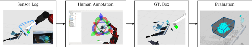
Figure 4: Segmentation evaluation pipeline. The ground truth (gt.) box is annotated by human, and overlap between voxels and the box is computed as the accuracy.

V-B1 Ground Truth Annotation

We evaluate our segmentation method with human annotation for ground truth as shown in Fig.4. The sensor log, camera and robotic joint states, are collected with rosbag , and ground truth (gt.) box is annotated using interactive markers [23] on rviz .

V-B2 Evaluation Metric

The metric is the three-dimensional intersect-over-union $IU_{3d}$ between the set of generated object voxels $V_{pred}$ and the box $V_{gt}$ with Equation V-B2, where the volume of voxels and box is calculated as $v_{pred}={\cal V}(V_{pred}),v_{gt}={\cal V}(V_{gt})$.

$$V_{tp}=V_{pred}\cap V_{gt},\quad v_{tp}={\cal V}(V_{tp})$$

$$v_{fp}=v_{pred}-v_{tp},\quad v_{fn}=v_{gt}-v_{tp}$$

$$IU_{3d}=\frac{v_{tp}}{v_{tp}+v_{fp}+v_{fn}}\qquad$$ (13)

This metric $IU_{3d}$ has value in range $[0,1]$, so we show value multiplied with 100 in following.

(a) View 1

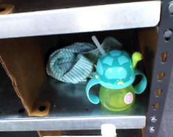
(b) View 2

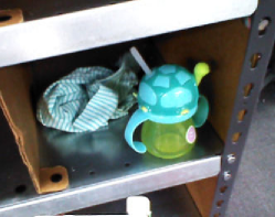
(c) View 3

Figure 5: Three views used in the evaluation.

V-B3 Result

We generate a looking-around motion with 3 different views shown in Fig.5, and the evaluation is conducted in situations with occlusions by object itself and the others. The result of projection-based method for both mean and max in views, is collected for each view and that based on LabelOctoMap is done after the views. Table VII shows the evaluation result with all 39 objects shown in Fig.3, and it shows our method (LabelOctoMap) exceeds conventional method (Projection) for 29 objects, and is close for 4 (label 7,14,27,34). The mapping result is worse than projection for 2 objects (25,26), which are both toothbrush with color difference. From this result, it is conceivable that our method is not efficient to segment objects which looks very similar and can have competitive probabilities, because the probabilities become relatively lower in that case than that when segmenting other objects. Results by both methods are similarly bad for 3 objects (5,30,31), and it can be said that this is mainly caused by lower accuracy of 2D segmentation (5,31) and insensible depth information of the objects because of its holes in the surface (30). These results are summarized in Table IV, and accuracy with our method exceeds that with projection-based method for both mean and max in views. These results show our mapping-based method is efficient to segment object three-dimensionally compared to the conventional projection-based method, and the validity of our proposed octomap which segments multiple objects in a multi-view action.

TABLE IV: Summary of segmentation results. They are the average of results ($IU_{3d}$) in Table VII.

methods	mean $IU_{3d}$
Projection (Mean)	6.40
Projection (Max)	8.98
LabelOctoMap	12.57

V-C Multi-Object Manipulation with Segmentation using LabelOctoMap

We evaluated real-time validity and applicability of our method in a multi-object manipulation task, which have the similar configuration as APC2016.

V-C1 Task Configuration

The manipulation task is conducted in a workspace shown in Fig.6, and the information below is given to the robot:

• Location and model of the shelf.

• Object set (Fig.3).

• Object names located each shelf bin.

• Name of the target object in each bin.

The purpose of the task is to pick the target object from the shelf bin and place it to the tote, so robot does not have to manipulate the non-target objects. However, since we located non-target objects with occluding the target object in all scenes, it is hard to pick the target without manipulating the obstacle objects. It is also allowed for the robot to move objects from a shelf bin to another, but information of the bin to which the object is moved must be noticed by the robot, because the information will be used another attempt of the task for the bin.

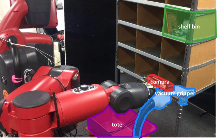
Figure 6: Workspace of the manipulation task. The location of each shelf bin and tote are given to the robot.

V-C2 Picking System Configuration

The overview of the picking system is shown in Fig.7. In detail, the task is conducted as follows:

1. Generate multilabel object voxels by LabelOctoMap with multi-view action.

2. Detect non-target objects in front of the target: centroids of each object-class voxels are computed, and robot decide to pick non-target object if its centroid is in front of the target object’s.

3. Remove outlier from voxels by euclidean clustering and fit bounding box.

4. Plan how to grasp: position is decided from centroid of the voxels, and orientation is decided from location and dimension of the box.

5. Remove or place the grasped object: non-target object is placed into empty bins, and target object is placed into the tote.

This task sequence is executed until the robot picks the target object and places into the designated place. In this manipulation scenario, it is assumed the location of the shelf bin and the name of target object are given.

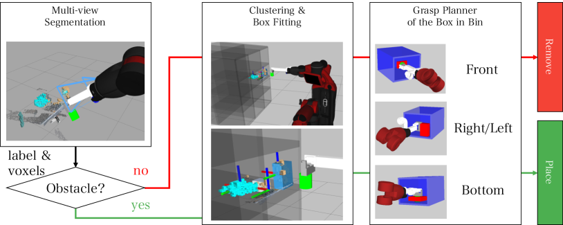
Figure 7: Picking system. The picking system includes multi-object manipulation, in order to remove obstacle objects to pick a target object.

V-C3 Result

Fig.8 shows the sequential frames of task in environment with 1 target and 3 obstacle objects, where the robot needs to remove the obstacle objects in order to pick the target object which is occluded. The robot successfully moved the obstacle objects to other shelf bin, and picked the target object and placed into the order bin.

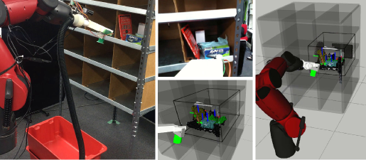
(a) Look around

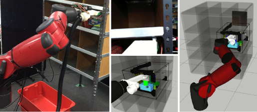
(b) Pick non target objects

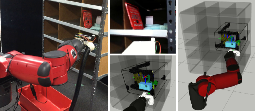
(c) Remove non target objects

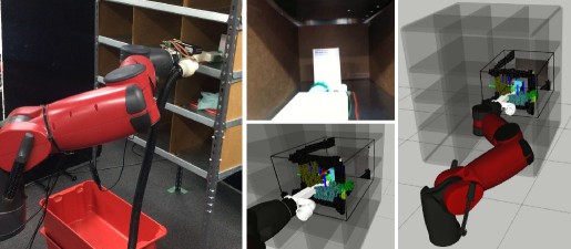
(d) Pick the target object

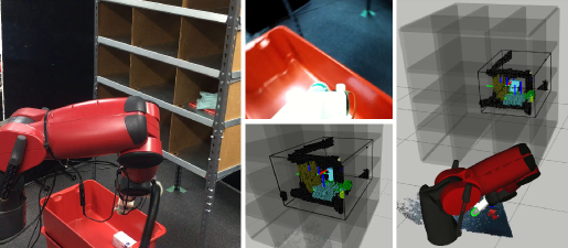
(e) Place the target object

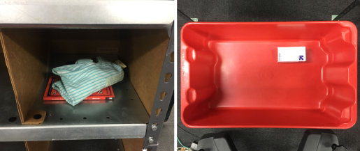
(f) Result

Figure 8: Sequential frames of the picking task. The frame shows the state of real robot (left), hand camera image (upper center), and visualization (lower center, right) in which colored voxels are the segmented objects and the axes represent the centroids.

We evaluated the efficiency of the picking system with proposed method by testing in 61 times picking task execution with 1 obstacle and 1 target object. The combination of 2 objects is randomly selected from 15 objects (2,4,6,7,10,14,22,24,27,28,34-36,38,39), which can be grasped relatively easily by the robot with a vacuum gripper. The environment is set to put an obstacle object in front of the target object. Table V shows the success rate, and Table VI shows some examples with scene image and task result: recognize is finding target and non-target, remove is moving non-target, and pick is picking target. The failure cases of remove and pick happen with gripper air leakage caused by inappropriate grasp location, and that of recognize happen with mistakenly detected non-target objects. In the experiment, the task, which includes multi-object manipulation in environment with occlusions, is achieved (in $\sim$60%), and this shows the applicability of our 3D segmentation method.

TABLE V: Success rate of the picking task.

	success rate	success rate (total)
recognize	86.9% (53/61)	86.9% (53/61)
remove	88.7% (47/53)	77.0% (47/61)
pick	78.7% (37/47)	60.7% (37/61)

TABLE VI: Recognition and task results. It shows scenes with different task results: recognize, remove, and pick.

	scene	segmentation	recog- nize	remove	pick
scene 1			✓	✓	✓
scene 2			✓	✓	✗
scene 3			✓	✗	—
scene 4			✗	—	—

TABLE VII: Segmentation results of the 39 objects used at APC2016. The blue box in images indicates the target object for segmentation, and bold text in table highlights the maximum, underline does competitive, and no decoration means all low accuracies (less than 1) in each row. The correnpondence between voxel color and label value is same as that shown in Table III.

	$IU_{3d}$			Scene	Result (LabelOctoMap)
	Projec- tion (Mean)	Projec- tion (Max)	Label- Octo- Map
label
1	7.81	10.74	16.11
2	5.35	7.93	12.99
3	8.68	10.05	15.94
4	2.10	4.91	5.39
5	0.07	0.36	0.05
6	11.14	14.02	32.78
7	6.76	18.30	18.28
8	3.50	5.58	10.61
9	1.16	2.40	4.83
10	9.44	12.56	17.77
11	4.59	10.86	14.16
12	3.16	3.92	7.10
13	12.26	14.21	21.36
14	10.19	16.68	16.41
15	0.00	0.00	0.00
16	5.54	8.78	12.41
17	5.92	6.83	13.53
18	3.80	4.41	7.34
19	7.08	8.47	11.62
20	1.45	2.59	3.65

	$IU_{3d}$			Scene	Result (LabelOctoMap)
	Projec- tion (Mean)	Projec- tion (Max)	Label- Octo- Map
label
21	1.58	2.09	3.78
22	4.40	5.25	9.28
23	4.53	5.28	9.95
24	16.47	19.92	31.43
25	1.14	4.44	0.59
26	9.32	15.42	11.61
27	4.69	10.86	10.79
28	4.12	5.33	9.16
29	11.15	13.32	17.06
30	0.01	0.10	0.02
31	0.02	0.19	0.00
32	11.20	12.53	19.25
33	6.62	12.54	15.74
34	3.72	5.62	5.50
35	16.18	17.90	20.07
36	21.07	24.00	36.99
37	5.81	8.15	12.19
38	17.53	22.70	33.32
39	0.22	0.95	1.81

VI Conclusions

We presented a method to segment multilabel objects in real world three-dimensionally, generating object voxels with probabilistic object label representation. The contributions of this paper are: 1) proposed a 3D segmentation method with mapping multilabel occupancy in real-time 2) evaluated the applicability of the segmentation method in the multi-object manipulation experiment. By using the proposed method, we achieved 3D multi-class segmentation in environments with occlusions, and picking task which requires multi-object manipulation.

The future work would be the extension of the proposed method to object instances in the same object class, because currently the method is unable to segment multiple instances if they are close to each other. The optimization of viewpoints and extension to dynamic objects which moves during multi-view also should be addressed.

References

- [1] Kentaro Wada, Masaki Murooka, Kei Okada, and Masayuki Inaba. 3d object segmentation for shelf bin picking by humanoid with deep learning and occupancy voxel grid map. In Humanoid Robots (Humanoids), 2016 IEEE-RAS 16th International Conference on, pp. 1149–1154. IEEE, 2016.
- [2] Matei Ciocarlie, Kaijen Hsiao, Edward Gil Jones, Sachin Chitta, Radu Bogdan Rusu, and Ioan A Şucan. Towards reliable grasping and manipulation in household environments. In Experimental Robotics, pp. 241–252. Springer, 2014.
- [3] Armin Hornung, Kai M Wurm, Maren Bennewitz, Cyrill Stachniss, and Wolfram Burgard. Octomap: An efficient probabilistic 3d mapping framework based on octrees. Autonomous Robots, Vol. 34, No. 3, pp. 189–206, 2013.
- [4] Jörg Stückler, Nenad Biresev, and Sven Behnke. Semantic mapping using object-class segmentation of rgb-d images. In Intelligent Robots and Systems (IROS), 2012 IEEE/RSJ International Conference on, pp. 3005–3010. IEEE, 2012.
- [5] Carsten Rother, Vladimir Kolmogorov, and Andrew Blake. Grabcut: Interactive foreground extraction using iterated graph cuts. In ACM transactions on graphics (TOG), Vol. 23, pp. 309–314. ACM, 2004.
- [6] Ning Xu, Narendra Ahuja, and Ravi Bansal. Object segmentation using graph cuts based active contours. Computer Vision and Image Understanding, Vol. 107, No. 3, pp. 210–224, 2007.
- [7] Brian Fulkerson, Andrea Vedaldi, and Stefano Soatto. Class segmentation and object localization with superpixel neighborhoods. In Computer Vision, 2009 IEEE 12th International Conference on, pp. 670–677. IEEE, 2009.
- [8] Stephen Gould, Jim Rodgers, David Cohen, Gal Elidan, and Daphne Koller. Multi-class segmentation with relative location prior. International Journal of Computer Vision, Vol. 80, No. 3, pp. 300–316, 2008.
- [9] Clemens Eppner, Sebastian Höfer, Rico Jonschkowski, Roberto Martın-Martın, Arne Sieverling, Vincent Wall, and Oliver Brock. Lessons from the amazon picking challenge: Four aspects of building robotic systems. Proceedings of Robotics: Science and Systems, AnnArbor, Michigan, 2016.
- [10] Jonathan Long, Evan Shelhamer, and Trevor Darrell. Fully convolutional networks for semantic segmentation. In Proceedings of the IEEE Conference on Computer Vision and Pattern Recognition, pp. 3431–3440, 2015.
- [11] Vijay Badrinarayanan, Alex Kendall, and Roberto Cipolla. Segnet: A deep convolutional encoder-decoder architecture for image segmentation. arXiv preprint arXiv:1511.00561, 2015.
- [12] Andy Zeng, Kuan-Ting Yu, Shuran Song, Daniel Suo, Ed Walker Jr, Alberto Rodriguez, and Jianxiong Xiao. Multi-view self-supervised deep learning for 6d pose estimation in the amazon picking challenge. arXiv preprint arXiv:1609.09475, 2016.
- [13] Ajmal S Mian, Mohammed Bennamoun, and Robyn Owens. Three-dimensional model-based object recognition and segmentation in cluttered scenes. IEEE transactions on pattern analysis and machine intelligence, Vol. 28, No. 10, pp. 1584–1601, 2006.
- [14] Stefan Hinterstoisser, Stefan Holzer, Cedric Cagniart, Slobodan Ilic, Kurt Konolige, Nassir Navab, and Vincent Lepetit. Multimodal templates for real-time detection of texture-less objects in heavily cluttered scenes. In Computer Vision (ICCV), 2011 IEEE International Conference on, pp. 858–865. IEEE, 2011.
- [15] Aitor Aldoma, Markus Vincze, Nico Blodow, David Gossow, Suat Gedikli, Radu Bogdan Rusu, and Gary Bradski. Cad-model recognition and 6dof pose estimation using 3d cues. In Computer Vision Workshops (ICCV Workshops), 2011 IEEE International Conference on, pp. 585–592. IEEE, 2011.
- [16] Radu Bogdan Rusu, Nico Blodow, and Michael Beetz. Fast point feature histograms (fpfh) for 3d registration. In Robotics and Automation, 2009. ICRA’09. IEEE International Conference on, pp. 3212–3217. IEEE, 2009.
- [17] Tomonari Furukawa, Frederic Bourgault, Benjamin Lavis, and Hugh F Durrant-Whyte. Recursive bayesian search-and-tracking using coordinated uavs for lost targets. In Robotics and Automation, 2006. ICRA 2006. Proceedings 2006 IEEE International Conference on, pp. 2521–2526. IEEE, 2006.
- [18] Alberto Elfes. Using occupancy grids for mobile robot perception and navigation. Computer, Vol. 22, No. 6, pp. 46–57, 1989.
- [19] Bogdan Moldovan, Plinio Moreno, Martijn van Otterlo, José Santos-Victor, and Luc De Raedt. Learning relational affordance models for robots in multi-object manipulation tasks. In Robotics and Automation (ICRA), 2012 IEEE International Conference on, pp. 4373–4378. IEEE, 2012.
- [20] Kensuke Harada, Jun Nishiyama, Yoshihiro Murakami, and Makoto Kaneko. Pushing manipulation for multiple objects. Journal of dynamic systems, measurement, and control, Vol. 128, No. 2, pp. 422–427, 2006.
- [21] Joni Pajarinen and Ville Kyrki. Robotic manipulation of multiple objects as a pomdp. Artificial Intelligence, 2015.
- [22] Rico Jonschkowski, Clemens Eppner, Sebastian Höfer, Roberto Martín-Martín, and Oliver Brock. Probabilistic multi-class segmentation for the amazon picking challenge. In Intelligent Robots and Systems (IROS), 2016 IEEE/RSJ International Conference on, pp. 1–7. IEEE, 2016.
- [23] David Gossow, Adam Leeper, Dave Hershberger, and Matei Ciocarlie. Interactive markers: 3-d user interfaces for ros applications [ros topics]. IEEE Robotics & Automation Magazine, Vol. 18, No. 4, pp. 14–15, 2011.