Resilient quantum electron microscopy

Abstract

We investigate the fundamental limit of biological quantum electron microscopy, which is designed to go beyond the shot noise limit. Inelastic scattering is expected to be the main obstacle in this setting, especially for thick specimens of actual biological interest. Here we describe a measurement procedure that, in principle, significantly neutralizes the effect of inelastic scattering.

I Introduction

The raw resolution of biological electron cryomicroscopy (cryoEM) is manifestly limited by shot noise. This is due to the small number of imaging electrons intended for avoiding radiation damage to the frozen specimen henderson_review (1). In single particle analysis (SPA), for instance, the tolerable number of electrons, i.e. the electron fluence, is at most $\approx 5\times 10^{3}/\mathrm{nm^{2}}$ grant grigorieff (2). On the other hand, biological objects are weak phase objects. Hence shot noise tends to bury the signal and thus limits the attainable resolution.

Quantum metrology, where phase measurement is a standard problem, is a natural approach to improving cryoEM. Recall that measuring a small phase $\theta$ with precision $\delta\theta$ takes $N\approx\delta\theta^{-2}$ electrons because of the shot noise limit. There have recently been proposals of quantum electron microscopy (QEM) schemes for approaching the Heisenberg limit, where $N\approx\delta\theta^{-1}$. Some quantum schemes are based on repeated use of single electrons Bob_phys_today (3, 4, 5, 6, 7, 8, 9, 10), while others use entanglement between electrons and superconducting qubits eeem_cpb (11, 12, 13). Nonetheless, many of these methods accumulate the small phase $\theta$ onto a quantum object $k$ times, resulting in a phase $k\theta$ after $k$ electron-passing events through the specimen, which is then measured. Call this process a single round of measurement, and call $k$ the repetition number. This is equivalent to measuring a hypothetical object with associated phase shift $k\theta$, using hypothetical $N/k$ probe particles at the shot noise limit. As a result, we obtain an increased effective number of electrons as $kN\approx\delta\theta^{-2}$, which approaches the Heisenberg limit at $k=N$. However, the usable value of $k$ depends on the frequency of inelastic scattering. If inelastic scattering destroys a round of measurement, then all electron passages used in that round are wasted.

In this work, we explore the limit of QEM. We ask a question, “Can we neutralize the adverse effect of inelastic scattering at least partially?”, and give an affirmative answer. To explore the physical limit, as opposed to the engineering limit, we assume the full ability to manipulate and measure the combined system of imaging electrons and other quantum objects. Without loss of generality, “other quantum objects” may be thought of as a set of qubits. In short, we consider an electron microscope connected to a quantum computer, which we may call a universal QEM q_interface (14).

The raw resolution of current cryoEM is about $3-5\,\mathrm{nm}$ raw resolution cryoET (15). All high resolution data to date are obtained only by averaging over at least tens of thousands of molecules of the same structure, by using e.g. SPA. However, the biologist would ultimately want to see molecules in their cellular context, rather than as ensemble average of purified molecules. We focus on unique, single specimens in the present work. At present, only very large proteins ($\sim$MDa) are identifiable in electron cryotomography (ECT) baumeister_review (16). High energy electrons generally are desirable in ECT to ensure transmission of electrons especially when the specimen is tilted. Moreover, the effective thickness of the specimen is $k$ times the actual thickness in QEM. Hence, hereafter we focus on $300\,\mathrm{keV}$ electrons with the wavelength $\lambda=1.97\,\mathrm{pm}$.

The specimen thickness $t$ is an important parameter in QEM. As quantum measurement is limited by lossy events, a relevant length to be compared with $t$ is the inelastic mean free path $\Lambda=200-350\,\mathrm{nm}$ for $300\,\mathrm{keV}$ electrons vulovic_etal (17). Suppose, for now, that all inelastic scattering destroy quantum measurement. The fraction of quantum measurements that survive to the end is $e^{-kt/\Lambda}$ because of $k$ electron passing events. Hence we replace the number of rounds $N/k$ with $Ne^{-kt/\Lambda}/k$. We thus modify the above relation $kN\approx\delta\theta^{-2}$ to $kNe^{-kt/\Lambda}\approx\delta\theta^{-2}$. The optimal $k$ that maximizes $\delta\theta^{-2}$ is $k_{1}=\Lambda/t$, where we have a relation $\delta\theta\approx\sqrt{e/k_{1}N}$. Improvement over the shot noise limit $\delta\theta\approx 1/\sqrt{N}$ in terms of the phase measurement precision is therefore

$$\sqrt{\frac{k_{1}}{e}}=\sqrt{\frac{\Lambda}{et}}\approx\sqrt{\frac{100\,\mathrm{nm}}{t}}.$$ (1)

This result emphasizes the importance of thinning the specimen. However, perhaps $t$ cannot be smaller than the size of biological molecules, e.g. $\approx 10\,\mathrm{nm}$. Moreover, in cryoEM of vitreous sections (CEMOVIS), the specimen thickness is “rarely less than $50\,\mathrm{nm}$” CEMOVIS sample thickness (18). Hence, to attain sizable improvement, we must neutralize the effect of inelastic scattering, which is the central topic of this paper.

We list some conventions. We generally represent the length of a vector, for example $\mathbf{a}$, using the same symbol, i.e. $a=|\mathbf{a}|$. Symbols $\hat{\mathbf{i}},\,\hat{\mathbf{j}},\,\hat{\mathbf{k}}$ denote unit vectors parallel to $x,\,y$ and $z$ axes, respectively. The electron optical axis is $z$. A position in real space is represented as $\mathbf{r}=x\hat{\mathbf{i}}+y\hat{\mathbf{j}}+z\hat{\mathbf{k}}$. A wave vector in the reciprocal space is written as $\mathbf{k}=k_{x}\hat{\mathbf{i}}+k_{y}\hat{\mathbf{j}}+k_{z}\hat{\mathbf{k}}$. Its size is related to the wavelength $\lambda$ as $k=2\pi/\lambda$, as opposed to the crystallographic definition $k=1/\lambda$. In many cases, we only need projections of vectors onto the $xy$-plane, which are represented by the same symbols when there is no danger of confusion. Eigenstates of the position and momentum operators are $|\mathbf{r}\rangle$ and $|\mathbf{k}\rangle$, respectively. We will often use $2$-dimensional (2d) Fourier transform (FT) and its inverse:

$$F\left(\mathbf{k}\right)=\mathcal{F}_{C}\left\{f\left(\mathbf{r}\right)\right\}=\int f\left(\mathbf{r}\right)e^{-i\mathbf{k}\cdot\mathbf{r}}d^{2}\mathbf{r},$$ (2)

$$f\left(\mathbf{r}\right)=\mathcal{F}_{C}^{-1}\left\{F\left(\mathbf{k}\right)\right\}=\int F\left(\mathbf{k}\right)e^{i\mathbf{k}\cdot\mathbf{r}}\frac{d^{2}\mathbf{k}}{\left(2\pi\right)^{2}},$$ (3)

where the subscript $C$ denotes “continuous” of continuous FT. When there is no risk of confusion, a tensor product $|a\rangle\otimes|b\rangle$ is simply written as $|a\rangle|b\rangle$ or $|ab\rangle$. The rest mass of the electron is denoted as $m_{e}$. We use conventional relativistic notations $\beta=\frac{v}{c}$ and $\gamma=\frac{1}{\sqrt{1-\beta^{2}}}$. Additional conventions are presented at relevant places.

II Resolution-dependent specimen damage

Specimen damage starts from short-range structural features progressively towards long-range features. A recent transmission electron microscopy (TEM) study Russo (19) on a purple membrane 2d crystal describes radiation damage in a way that is particularly amenable to theoretical analysis. Let the scattering vector be $\mathbf{q}=\mathbf{k}_{f}-\mathbf{k}_{i}$, where $\mathbf{k}_{i},\,\mathbf{k}_{f}$ are electron wave vectors before and after scattering. The vector $\mathbf{q}$ is practically perpendicular to the optical axis $z$ and we will occasionally treat $\mathbf{q}$ as a $2$d vector in the $q_{x}q_{y}$-plane. The intensity of the electron wave scattered off the crystal at a diffraction plane is found to decay as Russo (19)

$$I=I_{0}e^{-RFq^{2}/8\pi^{2}},$$ (4)

where $I$ is the intensity, $I_{0}$ is the initial intensity, $R\approx 7\times 10^{-4}\mathrm{nm}^{4}$ is a constant, $F$ is electron fluence. The initial intensity $I_{0}$ is proportional to $\varSigma_{0}e^{-R_{g}^{2}q^{2}/3}$, as usually found in the Guinier plot, where $R_{g}$ is the radius of gyration of the molecule under study rosenthal_henderson (20). However, at higher spatial frequencies, scattered waves from atoms interfere essentially at random, giving constant average intensity with respect to $\mathbf{q}$ that is the sum of intensities from each atom, with random phase. Although the particular value of $R$ above pertains to the purple membrane, we assume that the value generalizes fairly well to other proteins.

The “$B$-factor” $B=RF$ has a natural interpretation that electron irradiation basically causes random walks of atoms, recalling that the standard $B$-factor in X-ray crystallography expresses the square of thermal atomic displacements. Indeed, we show that $\sqrt{B/8\pi^{2}}$ may be regarded as the expected positional deviation of atoms from the original location. Let the position and the electron scattering amplitude (having the dimension of length) of $s$-th atom be $\mathbf{r}_{s}$ and $f_{s}$, respectively. Our argument is valid to the extent that $f_{s}$ can be regarded as a constant within the range of scattering angle of interest. The scattered electron wavefunction amplitude $\psi\left(\mathbf{q}\right)$ in the far field is proportional to

$$\psi\left(\mathbf{q}\right)\propto\sum_{s}f_{s}e^{-i\mathbf{q}\cdot\mathbf{r}_{s}}.$$ (5)

In the present case the scattering vector $\mathbf{q}$ lies almost exactly in a plane perpendicular to the optical axis. Hence we treat $\mathbf{q}$, as well as $\mathbf{r}_{s}$, as 2-dimensional. Introducing a function $\gamma\left(\mathbf{r}\right)$ representing the projected “density of the scattering amplitude”, we obtain

$$\psi\left(\mathbf{q}\right)\propto\int d^{2}\mathbf{r}\gamma\left(\mathbf{r}\right)e^{-i\mathbf{q}\cdot\mathbf{r}}.$$ (6)

Suppose that atoms random walk. We model this process by convoluting the projected density of scattering amplitude $\gamma\left(\mathbf{r}\right)$ with

$$g\left(\mathbf{r}\right)=\frac{1}{2\pi d^{2}}e^{-\frac{x^{2}+y^{2}}{2d^{2}}}$$ (7)

upon irradiation, where $d$ is the standard positional displacement from the initial positions of atoms. Fourier transforming, we obtain the scattering amplitude that is $\psi\left(\mathbf{q}\right)$ multiplied by $\mathcal{F}_{C}\left\{g\left(\mathbf{r}\right)\right\}=e^{-\frac{d^{2}q^{2}}{2}}$. Hence the initial intensity $I_{0}=\left|\psi\left(\mathbf{q}\right)\right|^{2}$ at zero radiation damage is multiplied by $e^{-d^{2}q^{2}}$. This allows us to identify $d^{2}$ with $B/8\pi^{2}$.

Finally, we note a limitation of this approach. We implicitly assumed that there are many atoms random-walking so that $\gamma\left(\mathbf{r}\right)$ may be considered to be convoluted with a gaussian function. After a long time, all the intensity on the diffraction plane is concentrated at $\mathbf{q}=0$ in this model. However, all the atoms should remain at some particular positions rather than having smoothed out by gaussian averaging. Hence random intensity in the far field should remain.

III The measurement procedure

III.1 High-level ideas

We begin with a high-level description of our measurement procedure. Since small structural features disappear fast, it is sensible to selectively acquire high spatial frequency (SF) data first. Selective-SF measurement makes sense also in view of inelastic scattering because high-SF measurements, associated with high-angle scattering, tend to be insensitive to small-angle inelastic scattering for reasons to be described later. Hence our strategy is to repeat measurement of scattered-wave amplitude at a specific SF, beginning at a large $q$ region and progressively moving inwards in the far field. We show that universal QEM, irrespective of the physical system it is based on, allows for such selective-SF measurement. However, selective-SF measurement may most easily be understood as an extended version of entanglement-enhanced electron microscopy (EEEM, see Appendix A) based on superconducting qubits.

We suppress unwanted signals outside the chosen SF by not performing phase-to-amplitude conversion and by not quantum-enhance them. As discussed in the previous section, unwanted low-resolution signals tend to be larger than the high-resolution signal we are after in typical biological specimens. Such unwanted large signal adversely interfere with high resolution measurement because the relation between the phase shift to contrast is not exactly linear in phase contrast microscopy.

The allowable fluence at each SF is rigidly constrained. Let $A$ be the area of electron beam illumination and define $\sigma=\frac{\pi}{q}$ as the resolution of interest. Since $B/8\pi^{2}=RF/8\pi^{2}$ is essentially the mean squared distance traveled by random-walking atoms under electron irradiation, structural information on the length scale $\sigma$ should be obtained before $\sigma^{2}\approx B/8\pi^{2}$, i.e. electron fluence $F$ reaches $F_{\mathrm{opt}}=\zeta\frac{8\pi^{2}\sigma^{2}}{R}$, where $\zeta=O\left(1\right)$ is a numerical constant.

We briefly digress to give an argument that gives $\zeta=0.255$ as a plausibly optimal numerical value. The overall physical picture is that too small a fluence $F$ gives no statistical confidence, while too large an $F$ yields data that mostly reflect altered structures due to radiation damage. Hence an optimal $F_{\mathrm{opt}}$ should exist. To find a useful $\zeta$ value, we make a pragmatic assumption that a Fourier component $\theta_{\mathbf{q}}$ of the real-space map of weak phase shift $\theta\left(\mathbf{r}\right)$ of the specimen decays to zero as $\theta_{\mathbf{q}}\left(F\right)=\theta_{0}e^{-F/F_{0}}$ for some $F_{0}$. Strictly speaking, this assumption cannot be entirely right (see the last paragraph of Sec. II) but we hope to obtain a useful estimate nonetheless. As shown in the quantitative study of radiation damage Russo (19), $\theta_{\mathbf{q}}^{2}$ is proportional to the diffraction intensity $I\left(\mathbf{q}\right)$ and hence

$$\theta_{\mathbf{q}}\left(F\right)=\theta_{0}e^{-RFq^{2}/16\pi^{2}}.$$ (8)

It follows that $F_{0}=\frac{16\pi^{2}}{Rq^{2}}=\frac{16\sigma^{2}}{R}\approx 2.3\times 10^{4}\,\mathrm{nm}^{-2}\cdot\left(\sigma/\mathrm{nm}\right)^{2}$. This is sufficiently large and unless we are after very high resolution data, we can ignore the specimen change during each round of quantum measurement, assuming the repetition number of the order of $k\approx\Lambda/t\approx 10$. Let $|s\rangle$ be the unscattered electron state and $|a\rangle$ be the scattered state with the wave vector $\mathbf{q}$. Deferring the question of how to perform SF-selective measurement, in principle we obtain a quantum state $|s\rangle+ik\theta_{\mathbf{q}}\left(F\right)|a\rangle$ after a quantum-enhanced measurement with the repetition number $k$, providing $k\theta_{\mathbf{q}}\left(F\right)\ll 1$ (Also see later discussions in this subsection). By expressing the state with measurement basis states $\left|\uparrow\right\rangle=\left[\left(1+i\right)|s\rangle+\left(1-i\right)|a\rangle\right]/2$ and $\left|\downarrow\right\rangle=\left[\left(1-i\right)|s\rangle+\left(1+i\right)|a\rangle\right]/2$, we obtain the corresponding probabilities $p_{\uparrow}=\frac{1}{2}-k\theta_{\mathbf{q}}\left(F\right)$ and $p_{\downarrow}=\frac{1}{2}+k\theta_{\mathbf{q}}\left(F\right)$. Let $X$ be a random variable that represents the number of events “$\uparrow$” occurring after $N_{g}=AF/k$ quantum enhanced measurements on a specimen area $A$, each using a group of $k$ electrons. Note that $p_{\uparrow}$ is a function of $F$ and hence that of $N_{g}$, because the specimen gradually gets damaged. The expectation value $\overline{X}$ is given by

$$\overline{X}=\int p_{\uparrow}\left(N_{g}\right)dN_{g}\approx\frac{N_{g}}{2}-k\theta_{0}\int_{0}^{N_{g}}e^{-kN^{\prime}_{g}/AF_{0}}dN^{\prime}_{g}$$

$$=\frac{N_{g}}{2}-AF_{0}\theta_{0}\left(1-e^{-kN_{g}/AF_{0}}\right),$$ (9)

while the variance is approximately a constant with respect to $\theta_{0}$, i.e.

$$\mathrm{Var}\left(X\right)=\int_{0}^{N_{g}}p_{\uparrow}\left(N_{g}^{\prime}\right)p_{\downarrow}\left(N_{g}^{\prime}\right)dN_{g}^{\prime}\approx\frac{N_{g}}{4}.$$ (10)

The estimator for $\theta_{0}$ is

$$\hat{\theta}_{0}\left(X\right)=\frac{\nu/k}{1-e^{-\nu}}\left(\frac{1}{2}-\frac{X}{N_{g}}\right),$$ (11)

where $\nu=kN_{g}/AF_{0}=F/F_{0}$. We obtain

$$\mathrm{Var}\left(\hat{\theta}_{0}\left(X\right)\right)\approx\frac{1}{4kAF_{0}}\frac{\nu}{\left(1-e^{-\nu}\right)^{2}},$$ (12)

which is minimized at $\nu_{\mathrm{opt}}\approx 1.26$, where $e^{\nu}=2\nu+1$ is satisfied. Hence we obtain $\zeta=2F_{\mathrm{opt}}/\left(\pi^{2}F_{0}\right)=2\nu_{\mathrm{opt}}/\pi^{2}\approx 0.255$.

Having found an appropriate value of $\zeta$, we proceed to consider our highly constrained way to spend the fluence budget to each SF bands. The electron fluence that one can expend in a ring-shaped resolution band $\left[q,q+\Delta q\right]$ on the $q_{x}q_{y}$ plane is

$$\Delta F=F_{\mathrm{opt}}\left(q\right)-F_{\mathrm{opt}}\left(q+\Delta q\right)$$

$$\approx-\frac{dF_{\mathrm{opt}}\left(q\right)}{dq}\Delta q=\zeta\frac{16\pi^{4}}{Rq^{3}}\Delta q.$$ (13)

There are $\frac{2\pi q}{\Delta q}$ square-shaped regions with the side length $\Delta q$ in the band $\left[q,q+\Delta q\right]$ in the $q$-space. Thus, the fluence budget for the measurement at each square-shaped region is $F_{\mathrm{sq}}=\frac{\Delta F}{2\pi q/\Delta q}$. A natural scale of $\Delta q$ satisfies $A\cdot\Delta q^{2}=\left(2\pi\right)^{2}$, where $A$ is the imaging area in the real space, since we do not have structures finer than $\Delta q$ in the reciprocal space. Thus, we are allowed to spend electron dose

$$N_{\mathrm{sq}}=F_{\mathrm{sq}}A=\zeta\frac{32\pi\sigma^{4}}{R}=3.7\times 10^{4}\left(\sigma/\mathrm{nm}\right)^{4}$$ (14)

for measuring scattered wave amplitude at a small area $\Delta q^{2}$ in the $q$-space. This expression has a quartic dependence on $\sigma$, meaning that allowed fluence is much smaller at a higher SF. Note that Eq. (14) does not depend on the area $A$. The reason is that a large area in the real space is associated with a finer $\Delta q$ and hence many points need to be scanned in the reciprocal space.

In the rest of this section, we briefly sketch the method of acquiring data at a specific SF $\mathbf{q}$. To focus on the essence of the idea, consider 1-dimensional specimen and we write $\mathbf{q}=q\hat{\mathbf{i}}=\frac{\pi}{\sigma}\hat{\mathbf{i}}$. The specimen is a weak phase object and an incident wave $e^{ik_{z}z}$ is scattered into a state

$$e^{i\left[k_{z}z+\theta\left(x\right)\right]}\approx e^{ik_{z}z}\left[1+i\theta\left(x\right)\right],$$ (15)

where $\theta\left(x\right)\ll 1$ is the phase shift map that we want to determine. It is natural to assume that the process is insensitive to the tilt of the incident wave, and hence for a small $k$ we have

$$e^{i\left[k_{z}z+kx+\theta\left(x\right)\right]}\approx e^{i\left(k_{z}z+kx\right)}\left[1+i\theta\left(x\right)\right].$$ (16)

Henceforth we omit the common factor $e^{ik_{z}z}$. Let the incident electron state be superposition of plane waves with the $x$ component of wavevectors separated by $2q$:

$$\psi_{s}\left(x\right)=\sum_{n\in\mathbb{Z}}e^{2niqx}.$$ (17)

We will pretend that $n$ runs over all integers for mathematical convenience. Obviously this is an idealization because the aperture angle is finite and small in real electron optics. Since we focus on the SF $q$, we study scattering of the incident wave into a state

$$\psi_{a}\left(x\right)=\sum_{n\in\mathbb{Z}}e^{\left(2n+1\right)iqx},$$ (18)

which has wavevectors in the midpoints between those in the incident state. We made the incident waves lattice-like for symmetry reasons, as will be clear shortly. Note that $\psi_{s}\left(x\right)$ and $\psi_{a}\left(x\right)$ are both real.

Consider a specimen with $\theta\left(x\right)=\theta_{0}\cos\left(qx\right)$ for now to focus on the SF $q$. A plane wave precisely along the optical axis scatters into

$$1+i\theta\left(x\right)\approx 1+\frac{i\theta_{0}}{2}\left(e^{iqx}+e^{-iqx}\right)$$ (19)

Superposing this, and utilized the assumption that the scattering process is not sensitive to small tilt angles, we see that scattering makes the following transformation:

$$\psi_{s}\left(x\right)\Rightarrow\psi_{s}\left(x\right)+i\theta_{0}\psi_{a}\left(x\right),\;\psi_{a}\left(x\right)\Rightarrow\psi_{a}\left(x\right)+i\theta_{0}\psi_{s}\left(x\right).$$ (20)

An alternative way, which provides a complementary view, to derive Eq.(20) is the following. First, note that $\psi_{0}\left(x\right)=\psi_{s}\left(x\right)+\psi_{a}\left(x\right)$ and $\psi_{1}\left(x\right)=\psi_{s}\left(x\right)-\psi_{a}\left(x\right)$ are proportional to $\sum_{n\in\mathbb{Z}}\delta\left(x-2n\sigma\right)$ and $\sum_{n\in\mathbb{Z}}\delta\left(x-2n\sigma-\sigma\right)$, respectively. (To see this, one may either use a physical argument or the mathematical identity

$$\sum_{n\in\mathbb{Z}}e^{2\pi inx}=\sum_{n\in\mathbb{Z}}\delta\left(x-n\right).$$ (21)

) Hence $\psi_{0}\left(x\right)$ and $\psi_{1}\left(x\right)$ should respectively receive phase shift $\theta_{0}$ and $-\theta_{0}$ because $\theta\left(x\right)=\theta_{0}\cos\left(qx\right)$. It follows that $\psi_{0}\left(x\right)\Rightarrow\psi_{0}\left(x\right)+i\theta_{0}\psi_{0}\left(x\right)$ and $\psi_{1}\left(x\right)\Rightarrow\psi_{1}\left(x\right)-i\theta_{0}\psi_{1}\left(x\right)$, which is consistent with Eq.(20). Starting with the initial state $\psi_{s}\left(x\right)$, we then repeat the transformation Eq.(20) for $k$ times. The final state should be $\psi_{s}\left(x\right)+ik\theta_{0}\psi_{a}\left(x\right)$ if $k\theta_{0}\ll 1$.

Next, consider general specimens. Unlike the specimen with the structure $\theta\left(x\right)=\theta_{0}\cos\left(qx\right)$, they scatter an incoming plane wave into all directions. Since we want to perform a selective SF measurement, we wish to confine the quantum state within the Hilbert subspace $\mathcal{H}$ spanned by $\psi_{s}\left(x\right)$ and $\psi_{a}\left(x\right)$. These two states are proportional to mutually interleaving rows of dots in the reciprocal $k$-space, namely $\sum_{n}\delta\left(k-2nq\right)$ for $\psi_{s}\left(x\right)$ and $\sum_{n}\delta\left(k-2nq-q\right)$ for $\psi_{a}\left(x\right)$. Scattering of the primary wave $\psi_{s}\left(x\right)$ into $\psi_{a}\left(x\right)$ is caused not only by the SF component $\pm q$, but also by those at $\pm 3q,\pm 5q,\cdots$. As we learned in Sec. II, higher-SF components are expected to be generally much smaller and hence we ignore them.

We begin with a SF-selective procedure with a poor performance, which is instructive nonetheless. We divide the reciprocal $k$-space into cells, that are intervals $\left[\left(n-\frac{1}{2}\right)q,\left(n+\frac{1}{2}\right)q\right)$, where $n\in\mathbb{Z}$. In other words, we reorganize $k$ into two variables $n$ and $-\frac{q}{2}\leq\hat{k}<\frac{q}{2}$, such that $k=nq+\hat{k}$ and hence $\hat{k}$ indicates the position within a cell. To remain in $\mathcal{H}$, we measure $\hat{k}$ but leave $n$ unmeasured. (This is conceptually not much different from measuring the $x$ coordinate of a particle while leaving its $y,z$ coordinates. Hence this should in principle be possible.) The measurement outcome would mostly be $\hat{k}=0$ because of the presence of the intense primary electron beam. In this case, a superposed state of $\psi_{s}\left(x\right)$ and $\psi_{a}\left(x\right)$ remains intact because both of these have the same value $\hat{k}=0$, although the parity of $n$ is different between these. On the other hand, if the measurement result is $\hat{k}\neq 0$, i.e. if elastic scattering takes place, the state such as $\psi_{s}\left(x\right)+ik\theta_{0}\psi_{a}\left(x\right)$ is destroyed. To see this, for example consider the similar amplitudes in the far field at $k=2nq+\hat{k}$ and $k=\left(2n+1\right)q+\hat{k}$, where $\hat{k}\approx\frac{q}{2}$. Hence the measurement fails. However, elastic scattering events take place sufficiently often and we cannot tolerate such a failure.

To remain in the space $\mathcal{H}$ after elastic scattering, we obfuscate the fact that elastic scattering ever happened. This is done by burying the scattered waves under the intense primary wave, by recombining these waves. Details are described in the next subsection, but what follows are some basic ideas. Since eventually we want to determine $\theta_{0}$ in the state $\psi_{s}\left(x\right)+ik\theta_{0}\psi_{a}\left(x\right)$, we do not want to recombine the scattered waves with $\psi_{s}\left(x\right)$ in such a way that $\psi_{s}\left(x\right)$ acquires the imaginary part. Recombination without such acquisition turns out to be possible because $\theta\left(x\right)$ is real, which in turn imply certain symmetry of the wave function in the reciprocal space. We note that this recombination process must involve a measurement, since the quantum state has unknown components outside the Hilbert subspace $\mathcal{H}$ but we need to project the state back to $\mathcal{H}$. As a bonus, such a measurement avoids coherently accumulating unwanted quantum amplitudes that do not belong the SF of interest. It turns out that a certain symmetry between $\psi_{s}\left(x\right)$ and $\psi_{a}\left(x\right)$ is desirable in our operations since we employ an extra quantum entity, namely a qubit. Hence, the recombination operation of the waves is performed separately in each cell $\left[n-\frac{q}{2},n+\frac{q}{2}\right)$. Eventually, we obtain a state of the form

$$\left(1+A\right)\psi_{s}\left(x\right)+\left(ik\theta_{0}+B\right)\psi_{a}\left(x\right),$$ (22)

where $A,B$ are real, unknown and small amplitudes coming from the undesirable scattered waves. We now argue that $A$ and $B$ does not present a significant problem. Consider the Bloch sphere, wherein $\psi_{0}\left(x\right)$ and $\psi_{1}\left(x\right)$ are north and south poles, respectively. To determine the imaginary component $ik\theta_{0}$, we want to measure the state with the measurement basis states $\psi_{\pm}\left(x\right)\propto\psi_{0}\left(x\right)\pm i\psi_{1}\left(x\right)$. Note that $\psi_{\pm}\left(x\right)$, $\psi_{s}\left(x\right)$, $\psi_{a}\left(x\right)$ and $\psi_{s}\left(x\right)+ik\theta\psi_{a}\left(x\right)$ are all on the equator of the sphere. Hence a measurement with respect to the basis $\psi_{\pm}\left(x\right)$ yields information about the longitude of the state on the Bloch sphere. Since small real values of $A,B$ mean a small shift in the latitude on the sphere, this will not significantly affect the measurement using the basis states $\psi_{\pm}\left(x\right)$.

Finally, we emphasize that the primary benefit of the SF-selective method discussed above lies in the handling of inelastic scattering. Since inelastic scattering tends to be associated with small scattering angles, separation of $\psi_{s}$ and $\psi_{a}$ in the far field helps us protect the quantum state that we need. See Sec. IV for further discussions.

III.2 Low-level procedure

We now describe details of the SF-selective measurement sketched above. Our selective-SF measurement procedure may be understood more smoothly if the reader knows how the “conventional” entanglement-enhanced electron microscopy (EEEM) works eeem_cpb (11, 12). See Appendix A for an introduction to EEEM.

We start with definitions. As in the previous subsection, we consider an incident electron state that form a lattice of focused beams on the specimen. However, this time the lattice is a 2d square lattice with the lattice constant $\sigma$. More specifically, let the number of focused beams be $M^{2}$, where $M=2^{j}$, where $j\geq 2$ is an integer. We define $k_{\mathrm{max}}=\frac{2\pi}{\sigma}$ and $k_{\mathrm{min}}=k_{\mathrm{max}}/M$. For later convenience, we define sets of ordered pairs of integers:

$$\mathcal{M}=\left\{\left(n,m\right)\in\mathbb{Z}^{2}|-\frac{M}{2}\leq n<\frac{M}{2},-\frac{M}{2}\leq m<\frac{M}{2}\right\},$$ (23)

$$\mathcal{M}_{s}=\left\{\left(n,m\right)\in\mathcal{M}|n<0\right\},$$ (24)

$$\mathcal{M}_{a}=\left\{\left(n,m\right)\in\mathcal{M}|0\leq n\right\},$$ (25)

$$\mathcal{M}_{c}=\left\{\left(n,m\right)\in\mathcal{M}|-\frac{M}{4}\leq n<\frac{M}{4}\right\},$$ (26)

$$\mathcal{M}_{e}=\left\{\left(n,m\right)\in\mathcal{M}|n\textrm{ is even}\right\},$$ (27)

and

$$\mathcal{M}_{o}=\left\{\left(n,m\right)\in\mathcal{M}|n\textrm{ is odd}\right\}.$$ (28)

Subscripts $s,a,c$ are intended to mean “symmetric”, “antisymmetric” and “center”, respectively. We also define singleton sets $\mathcal{C}_{s}=\left\{\left(-\frac{M}{4},0\right)\right\}$, $\mathcal{C}_{a}=\left\{\left(\frac{M}{4},0\right)\right\}$ and $\mathcal{C}_{c}=\left\{\left(0,0\right)\right\}$. The sets $\mathcal{C}_{s}$, $\mathcal{C}_{a}$ and $\mathcal{C}_{c}$, in a sense, contain the “central” element of $\mathcal{M}_{s}$, $\mathcal{M}_{a}$ and $\mathcal{M}_{c}$, respectively. Now, each focused electron beam is at $n\sigma\hat{\mathbf{i}}+m\sigma\hat{\mathbf{j}}$, where $\left(n,m\right)\in\mathcal{M}$. The electron state at the point $n\sigma\hat{\mathbf{i}}+m\sigma\hat{\mathbf{j}}$ is written as $|n,m\rangle$. Since a quantum state can in principle be transferred, but not copied, between the electron microscope and a connected quantum computer q_interface (14), the electron state $|n,m\rangle$ may equivalently be viewed, as we will do occasionally, as a state of two “registers of a quantum computer” $n,\,m$, each comprising $\log_{2}M$ qubits. They express integers $n,\,m$ in modified two’s complement notation (MTCN), wherein the sign bit is reversed: $0$ means negative and $1$ means positive. Let Q2 be the most significant qubit (MSQ) of the register $n$. The remaining part of the register $n$ is referred to as register $\tilde{n}$. The integer $\tilde{n}$ is represented again in MTCN and $-\frac{M}{4}\leq\tilde{n}<\frac{M}{4}$ is satisfied. Hence we have

$$\tilde{n}=\begin{cases}n+\frac{M}{4}&\textrm{if}\>-\frac{M}{2}\leq n<0\\ n-\frac{M}{4}&\textrm{if}\>0\leq n<\frac{M}{2}\end{cases}.$$ (29)

In addition to the registers $n,\,m$, we introduce an extra qubit Q1, which plays a central role.

We denote a state of a qubit with a bar. Let the basis states of a qubit be $|\overline{0}\rangle,\,|\overline{1}\rangle$. Define $|\overline{s}\rangle=\frac{|\overline{0}\rangle+|\overline{1}\rangle}{\sqrt{2}}$, $|\overline{a}\rangle=\frac{|\overline{0}\rangle-|\overline{1}\rangle}{\sqrt{2}}$, $|\overline{\uparrow}\rangle=\frac{|\overline{0}\rangle+i|\overline{1}\rangle}{\sqrt{2}}$ and $|\overline{\downarrow}\rangle=\frac{|\overline{0}\rangle-i|\overline{1}\rangle}{\sqrt{2}}$. The tensor product of an electron state $|p\rangle$ and the Q1 state $|\overline{q}\rangle$ will be denoted as $|p\rangle|\overline{q}\rangle$, or simply $|p\overline{q}\rangle$. Negative of complex conjugate will be abbreviated as NCC. Let $a_{n,m}$ be a set of $M^{2}$ values, where $\left(n,m\right)\in\mathcal{M}$. We write 2d discrete FT (DFT)

$$A_{n,m}=\frac{1}{M}\sum_{\left(r,s\right)\in\mathcal{M}}a_{r,s}e^{2\pi i\frac{nr+ms}{M}}$$ (30)

as $A_{n,m}=\mathcal{F}\left\{a_{n,m}\right\}$, where $\left(n,m\right)\in\mathcal{M}$. The inverse of the DFT is written as $a_{n,m}=\mathcal{F}^{-1}\left\{A_{n,m}\right\}$. The DFT is often applied to a set of quantum amplitudes as quantum FT (QFT Simon_qFFT (21)), wherein a state

$$\sum_{\left(n,m\right)\in\mathcal{M}}a_{n,m}|n,m\rangle$$ (31)

is converted to

$$\sum_{\left(n,m\right)\in\mathcal{M}}A_{n,m}|n,m\rangle,$$ (32)

where $A_{n,m}=\mathcal{F}\left\{a_{n,m}\right\}$. Here we further define split inverse FT, which applies inverse-FT individually to two half planes $\mathcal{M}_{s}$ and $\mathcal{M}_{a}$, wherein the central points are $\left(-\frac{M}{4},0\right)$ and $\left(\frac{M}{4},0\right)$, respectively. More specifically, $a_{n,m}=\mathcal{F}_{\textrm{split}}^{-1}\left\{A_{n,m}\right\}$ is a shorthand for

$$a_{n,m}=\frac{\sqrt{2}}{M}\sum_{\left(r,s\right)\in\mathcal{M}_{s}}A_{r,s}e^{-2\pi i\frac{2\left(r+\frac{M}{4}\right)\left(n+\frac{M}{4}\right)+sm}{M}},$$ (33)

for $\left(n,m\right)\in\mathcal{M}_{s}$, and

$$a_{n,m}=\frac{\sqrt{2}}{M}\sum_{\left(r,s\right)\in\mathcal{M}_{a}}A_{r,s}e^{-2\pi i\frac{2\left(r-\frac{M}{4}\right)\left(n-\frac{M}{4}\right)+sm}{M}},$$ (34)

for $\left(n,m\right)\in\mathcal{M}_{a}$. Alternatively, in accordance with Eq. (29)

$$a_{\tilde{n},m}=\frac{\sqrt{2}}{M}\sum_{\left(r,s\right)\in\mathcal{M}_{s}}A_{r,s}e^{-2\pi i\frac{2\left(r+\frac{M}{4}\right)\tilde{n}+sm}{M}}$$ (35)

if $n<0$, and

$$a_{\tilde{n},m}=\frac{\sqrt{2}}{M}\sum_{\left(r,s\right)\in\mathcal{M}_{a}}A_{r,s}e^{-2\pi i\frac{2\left(r-\frac{M}{4}\right)\tilde{n}+sm}{M}}$$ (36)

if $n\geq 0$, both for $\left(\tilde{n},m\right)\in\mathcal{M}_{c}$.

Three remarks about the split inverse FT are in order. First, the prefactor is $\frac{\sqrt{2}}{M}=\frac{1}{\sqrt{\frac{M^{2}}{2}}}$ because the number of elements involved in each FT is $\frac{M^{2}}{2}$. Second, the exponential factor may be rewritten as, e.g. when $\left(n,m\right)\in\mathcal{M}_{s}$,

$$e^{-2\pi i\frac{2\left(r+\frac{M}{4}\right)\left(n+\frac{M}{4}\right)+sm}{M}}=e^{-2\pi i\frac{\left(r+\frac{M}{4}\right)\left(n+\frac{M}{4}\right)}{M/2}}e^{-2\pi i\frac{sm}{M}}.$$ (37)

Third, from the QFT perspective, the above operation is equivalent to performing 2d inverse QFT on the state $|\tilde{n},m\rangle$, where we set aside the MSQ of the register $n$, i.e. Q2. Hence, we can define the split inverse QFT as a transformation of the state $\sum_{\left(\tilde{n},m\right)\in\mathcal{M}_{c}}A_{\tilde{n},m}|\tilde{n},m\rangle$ into $\sum_{\left(\tilde{n},m\right)\in\mathcal{M}_{c}}a_{\tilde{n},m}|\tilde{n},m\rangle$, where

$$a_{\tilde{n},m}=\frac{\sqrt{2}}{M}\sum_{\left(\tilde{r},s\right)\in\mathcal{M}_{c}}A_{\tilde{r},s}e^{-2\pi i\frac{2\tilde{r}\tilde{n}+sm}{M}}.$$ (38)

We consider a thin specimen that is characterized by a 2d phase shift map $\theta\left(x,y\right)$. The area of the measurement on the specimen is square-shaped, with the side length $L=M\sigma$. Define $\theta_{n,m}=\theta\left(n\sigma,m\sigma\right)$. We set

$$\sum_{\left(n,m\right)\in\mathcal{M}}\theta_{n,m}=0$$ (39)

without loss of generality. We aim to measure

$$\overline{\theta}=\frac{1}{M^{2}}\sum_{\left(n,m\right)\in\mathcal{M}}\left(-1\right)^{n}\theta_{n,m},$$ (40)

which obviously contains SF of $q=\frac{\pi}{\sigma}$ as the main component. That is, half the difference between; (A) the average value of $\theta_{n,m}$ with even $n$, and (B) the odd $n$ counterpart. The electron beam array being a square lattice is not particularly important. In addition, the reader may justifiably worry that a focused beam would quickly destroy the specimen at the focal point. A solution to this problem is discussed in Appendix B.

We are now ready to discuss the SF-selective measurement procedure. The electron state $|n,m\rangle$ after transmission through the specimen is

$$e^{i\theta_{n,m}}|n,m\rangle\approx\left(1+i\theta_{n,m}\right)|n,m\rangle$$ (41)

under weak phase approximation, where the small quantity $\theta_{n,m}$ is the phase map of a specimen. Define $\Theta_{n,m}=\mathcal{F}\left\{\theta_{n,m}\right\}$. Note that

$$\Theta_{0,0}=0$$ (42)

because of Eq. (39). Unlike the treatment in the previous subsection, in the following EEEM-like setting, we will deal with two symmetrically placed incident states

$$|s\rangle=\frac{1}{M}\sum_{\left(n,m\right)\in\mathcal{M}}e^{i\frac{\pi}{2}n}|n,m\rangle$$ (43)

and

$$|a\rangle=\frac{1}{M}\sum_{\left(n,m\right)\in\mathcal{M}}e^{-i\frac{\pi}{2}n}|n,m\rangle,$$ (44)

which are scattered into each other. (A change of the convention $|n,m\rangle\Rightarrow e^{-i\frac{\pi}{2}n}|n,m\rangle$ would make it better correspond to the “sketch” of the method in Sec. III.1. However, here we make $|s\rangle$ and $|a\rangle$ more symmetric.) These states interfere to make fringes at either even $n$ spots or odd ones, as in:

$$|0\rangle=\frac{|s\rangle+|a\rangle}{\sqrt{2}}=\frac{\sqrt{2}}{M}\sum_{\left(n,m\right)\in\mathcal{M}_{e}}\left(-1\right)^{\frac{n}{2}}|n,m\rangle,$$ (45)

$$|1\rangle=\frac{|s\rangle-|a\rangle}{\sqrt{2}}=\frac{\sqrt{2}i}{M}\sum_{\left(n,m\right)\in\mathcal{M}_{o}}\left(-1\right)^{\frac{n-1}{2}}|n,m\rangle.$$ (46)

Our intention is to measure the difference of the average phase shifts, of the transmitted electron beams, between locations belonging to $|0\rangle$ and $|1\rangle$ on the specimen. DFT transforms states in Eqs. (43) and (44) into $|-\frac{M}{4},0\rangle$ and $|\frac{M}{4},0\rangle$, respectively.

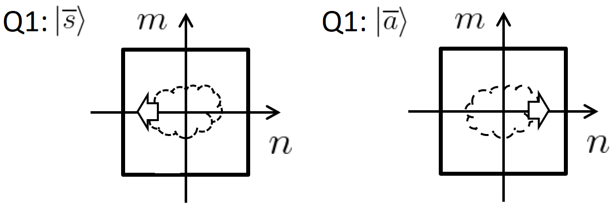
(a)

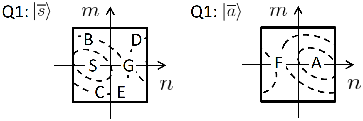
(b)

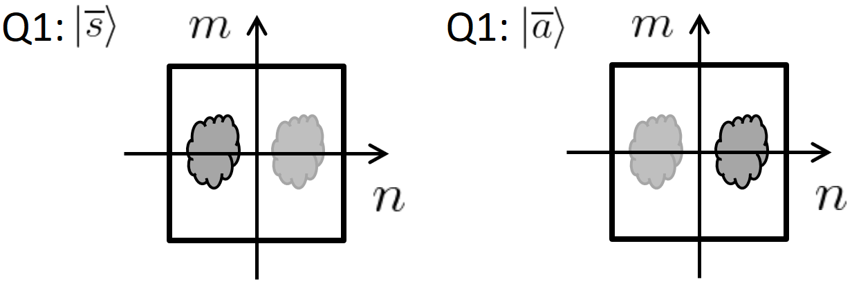
(c)

Figure 1: Illustrations of quantum states at different stages of spatial-frequency (SF) selective measurement. The electron state, which may have been transferred to a quantum computer, in the branch of the entire wavefunction, wherein Q1 state is $|\overline{s}\rangle$, is shown in the left figure. In a similar way, one with $|\overline{a}\rangle$ is on the right. See the main text for more information. (a) The state right after transmission of an electron through the specimen. The shape of the “molecule”, which is imprinted on the phase of electron wavefunction, is shown in dashed curves because it is not “visible”, in a loose analogy with transmission electron microscopy (TEM) imaging. The electron wavefront is such that the wave goes left if Q1 state is $|\overline{s}\rangle$, and goes right if Q1 state is $|\overline{a}\rangle$, as indicated by the arrows. (It reflects our convention of discrete Fourier transform.) (b) We apply QFT to the quantum states $|n,m\rangle$, representing the transmitted array of $M\times M$ beams, to obtain essentially a far-field state. The left-moving wave in figure (a) goes to point S, while the right-moving one goes to A. Elastically scattered waves, whose intensity is indicated by dashed curves, surround the transmitted waves at S and A. Unlike actual diffraction in real electron optics, periodic boundary condition (PBC) is applicable in quantum Fourier transform (QFT). Thus, the wave that goes beyond the left boundary, for example, comes out from the right side. The scattered amplitudes at B and C are the negative of complex conjugate (NCC) to each other. The same applies to D and E due to PBC. The amplitudes of interest at F and G are NCC to itself and hence is pure imaginary. These amplitudes at F and G are “added” to, although the wavefunction branch is different, the transmitted waves respectively at S and A with a $\frac{\pi}{2}$ phase difference. (c) The state after split inverse Fourier transformation (FT), where inverse FT is performed in $n<0$ and $n\geq 0$ regions separately. If the outcome of Q2 measurement in Step $7$ is $c=0$, the $n<0$ part of the map is left available, while for $c=1$, the $n\geq 0$ part remains. In each region, the shape of the “molecule” is recovered to an extent. In contrast to conventional in-focus phase contrast microscopy, we convert unwanted phase into amplitude in Step $6$ before the split inverse FT, because we want to accumulate the signal phase onto Q1. (In Step $12$, we measure Q1 with respect to basis states $\left\{|\overline{\uparrow}\rangle,|\overline{\downarrow}\rangle\right\}$, thus finally “converting the phase into amplitude”, figuratively speaking, when the final measurement is done.) Since the unwanted information is converted to amplitude and is “visible”, again in a loose analogy with TEM, the “molecules” are drawn with solid curves, as opposed to dashed curves that are found in figure (a). The images of the “molecule” is shown dimly when it is high-pass filtered, where the signal is indeed expected to be weak.

Figure 1 is designed to visualize aspects of the SF-selective measurement steps that we describe below. The combined system of the electron and Q1 has $2M^{2}$ complex amplitudes to specify its state (setting aside the minor issue of normalization and the overall phase), because the electron has $M^{2}$ basis vectors $|n,m\rangle$ and Q1 has $2$ basis vectors $|\overline{s}\rangle,\,|\overline{a}\rangle$. To visualize the state of the entire system, we can show two maps Q1:$|\overline{s}\rangle$ and Q1:$|\overline{a}\rangle$, each corresponding to $|\overline{s}\rangle$ and $|\overline{a}\rangle$ of the Q1 states, with $n$ and $m$ axes, to show a set of complex coefficients. For example, the point $\left(n,m\right)$ of the map for Q1:$|\overline{s}\rangle$ shows a complex coefficient, i.e. the quantum amplitude, for the state $|n,m\rangle|\overline{s}\rangle$. (To visualize complex numbers, one might use brightness and color to show the amplitude and phase, respectively, for example. However, we do not do such things in this paper, because schematic representations of general ideas suffice for us.)

We first state steps in SF-selective measurement without elucidating results of performing these steps.

Step $1$: Initialize the state of Q1 to be $|\overline{s}\rangle$.

Step $2$: Initialize the state of a new electron to $\frac{1}{\sqrt{2}}\left(|s\rangle+|a\rangle\right)$.

Step $3$: Apply a CNOT gate that flips Q1 state as $|\overline{s}\rangle\Leftrightarrow|\overline{a}\rangle$ if and only if the electron is in state $|a\rangle$.

Step $4$: Let the electron go through the specimen. Capture the electron quantum state in registers $n$ and $m$ of a quantum computer. (See Fig. 1 (a).)

Step $5$: Apply QFT that converts the amplitude of $|n,m\rangle$ from $a_{n,m}$ to $A_{n,m}=\mathcal{F}\left\{a_{n,m}\right\}$.

Step $6$: Multiply $i$ to two states $|\pm\frac{M}{4},0\rangle$ (i.e. points S, G, F, A in Fig. 1 (b)).

Step $7$: Measure Q2 with respect to basis $\left\{|\overline{0}\rangle,\,|\overline{1}\rangle\right\}$. Let the outcome be $c$. (Here we determine if the state is in the $n<0$, or $n\geq 0$, region of the map shown in Fig. 1 (b).)

Step $8$: Apply split inverse QFT. (See Fig. 1 (c). Also note that Q2 is not involved in this operation.)

Step $9$: Measure the state of the register $\tilde{n}$ (i.e. the register $n$ without Q2) and $m$ with respect to the basis $\left\{|\tilde{n},m\rangle|\left(\tilde{n},m\right)\in\mathcal{M}_{c}\right\}$. (Although the measurement outcome $\hat{n},\,\hat{m}$ contains low-resolution information, we do not discuss utilization of it in the present work.)

Step $10$: Apply the single-qubit operation $|\overline{s}\rangle\Leftrightarrow|\overline{a}\rangle$ to Q1 if and only if $c=1$.

Step $11$: Go back to step $2$ to repeat the process for $k$ times.

Step $12$: Measure Q1 with the basis states $\left\{|\overline{\uparrow}\rangle,|\overline{\downarrow}\rangle\right\}$. One obtains a single bit of data for one round of measurement.

In the rest of this section, we track the state of the microscope system during the above procedure. Anticipating later arguments, we write the Q1 state after Step $1$ in a generalized form

$$|\overline{s}\rangle+i\alpha|\overline{a}\rangle,$$ (47)

instead of simply writing it as $|\overline{s}\rangle$. Then, as specified in Step $2$ a new electron is prepared in the state

$$\frac{1}{\sqrt{2}}\left\{|s\rangle+|a\rangle\right\}.$$ (48)

Step $3$ is an entangling operation, which results in

$$\frac{1}{\sqrt{2}}\left\{\left(|s\overline{s}\rangle+|a\overline{a}\rangle\right)+i\alpha\left(|s\overline{a}\rangle+|a\overline{s}\rangle\right)\right\}.$$ (49)

In Step $4$, the electron goes through the specimen. The exit wave from the specimen generated from the incident wave $|s\rangle$ is

$$|\psi_{s}\rangle=\frac{1}{M}\sum_{\left(n,m\right)\in\mathcal{M}}\left(1+i\theta_{n,m}\right)e^{i\frac{\pi}{2}n}|n,m\rangle.$$ (50)

Likewise, for the incident wave $|a\rangle$ we obtain

$$|\psi_{a}\rangle=\frac{1}{M}\sum_{\left(n,m\right)\in\mathcal{M}}\left(1+i\theta_{n,m}\right)e^{-i\frac{\pi}{2}n}|n,m\rangle.$$ (51)

Thus, the state of the entire system, having captured the electron state in the quantum computer, is

$$\frac{1}{\sqrt{2}}\left\{\left(|\psi_{s}\overline{s}\rangle+|\psi_{a}\overline{a}\rangle\right)+i\alpha\left(|\psi_{s}\overline{a}\rangle+|\psi_{a}\overline{s}\rangle\right)\right\}$$ (52)

Figure 1 (a) schematically shows the state at this point. Both Q1:$|\overline{s}\rangle$ and Q1:$|\overline{a}\rangle$ maps show the same “biological molecule” imprinted as phase shift. However, the “wave fronts are tilted” in the opposite direction between these two maps because of the $e^{\pm i\frac{\pi}{2}n}$ factors in Eqs. (43, 44).

Next, in Step $5$, we perform 2d quantum fast Fourier transform (QFT) Simon_qFFT (21), which converts the amplitude $c_{n,m}$ of the state $|n,m\rangle$ to $c^{\prime}_{n,m}=\mathcal{F}\left\{c_{n,m}\right\}$. This amounts to moving to the diffraction plane, although the periodic boundary condition (PBC) applies here, unlike in the case of actual diffraction plane in real electron optics. Note two properties of Fourier-transformed phase map:

$$\Theta_{r+M,s}=\Theta_{r,s},$$ (53)

which is the PBC, and

$$\Theta_{r,s}=\Theta_{-r,-s}^{*},$$ (54)

because $\theta_{n,m}$ is real. Note that, due to Eq. (40),

$$\overline{\theta}=\frac{\Theta_{\frac{M}{2},0}}{M}=\frac{\Theta_{-\frac{M}{2},0}}{M},$$ (55)

which is what we aim to measure. QFT applied to $|\psi_{s}\rangle$ and $|\psi_{a}\rangle$ yields, taking Eq. (42) into account,

$$|\psi_{s2}\rangle=|-\frac{M}{4},0\rangle+\frac{i}{M}\sum_{\left(r,s\right)\in\mathcal{M}\backslash\mathcal{C}_{s}}\Theta_{r+\frac{M}{4},s}|r,s\rangle$$

$$=|-\frac{M}{4},0\rangle+i\overline{\theta}|\frac{M}{4},0\rangle+\frac{i}{M}\sum_{\left(r,s\right)\in\mathcal{M}\backslash\left(\mathcal{C}_{s}\cup\mathcal{C}_{a}\right)}\Theta_{r+\frac{M}{4},s}|r,s\rangle,$$ (56)

and

$$|\psi_{a2}\rangle=|\frac{M}{4},0\rangle+\frac{i}{M}\sum_{\left(r,s\right)\in\mathcal{M}\backslash\mathcal{C}_{a}}\Theta_{r-\frac{M}{4},s}|r,s\rangle$$

$$=|\frac{M}{4},0\rangle+i\overline{\theta}|-\frac{M}{4},0\rangle+\frac{i}{M}\sum_{\left(r,s\right)\in\mathcal{M}\backslash\left(\mathcal{C}_{s}\cup\mathcal{C}_{a}\right)}\Theta_{r-\frac{M}{4},s}|r,s\rangle.$$ (57)

The state of the entire system is thus

$$|\Psi_{1}\rangle=\frac{1}{\sqrt{2}}|-\frac{M}{4},0\rangle\left[\left(1-\alpha\overline{\theta}\right)|\overline{s}\rangle+i\left(\alpha+\overline{\theta}\right)|\overline{a}\rangle\right]+\frac{1}{\sqrt{2}}|\frac{M}{4},0\rangle\left[\left(1-\alpha\overline{\theta}\right)|\overline{a}\rangle+i\left(\alpha+\overline{\theta}\right)|\overline{s}\rangle\right]$$

$$+\frac{i}{\sqrt{2}M}\sum_{\left(r,s\right)\in\mathcal{M}\backslash\left(\mathcal{C}_{s}\cup\mathcal{C}_{a}\right)}|r,s\rangle\left\{\Theta_{r+\frac{M}{4},s}\left(|\overline{s}\rangle+i\alpha|\overline{a}\rangle\right)+\Theta_{r-\frac{M}{4},s}\left(|\overline{a}\rangle+i\alpha|\overline{s}\rangle\right)\right\}.$$ (58)

(To verify this, it may help to define and use $|\overline{p}\rangle=|\overline{s}\rangle+i\alpha|\overline{a}\rangle$ and $|\overline{q}\rangle=|\overline{s}\rangle+i\alpha|\overline{a}\rangle$.) Figure 1 (b) shows this state. In the first term of Eq. (58), the large component corresponds to the points S, while the smaller component corresponds to F. A similar statement can be made for the second term. The transmitted waves of the two “tilted incident waves” $|s\rangle,\,|a\rangle$ mainly make two points S and A in the far field. Elastically scattered waves are in the third term of Eq. (58) and surround these two points. They are shown in dashed curves in Fig. 1 (b). Because of Eq. (54), points B and C are NCC to each other. Moreover, the same can be said for points D and E because of Eq. (53).

To motivate the following steps, we first discuss a method of poor performance. Suppose that we measure the electron state at this point. If the measurement outcomes were always $n=\pm\frac{M}{4}$ and $m=0$, then, neglecting $\alpha\overline{\theta}$, we would be able to accumulate the phase $\overline{\theta}$ on top of $\alpha$ in Q1. However, sometimes we measure the electron state at other points $\left(r,s\right)$, when elastic scattering occurs. This would result in a Q1 state

$$\Theta_{r+\frac{M}{4},s}\left(|\overline{s}\rangle+i\alpha|\overline{a}\rangle\right)+\Theta_{r-\frac{M}{4},s}\left(|\overline{a}\rangle+i\alpha|\overline{s}\rangle\right),$$ (59)

which is basically a destroyed state unless one of $\Theta_{r+\frac{M}{4},s},\,\Theta_{r-\frac{M}{4},s}$ is overwhelmingly larger than the other, in the sense that the absolute value of their ratio (or its inverse) has to be much smaller than $\alpha$, which is generally small to begin with. To avoid such a scenario, we perform the following steps to obscure the fact that elastic scattering happened.

Hence in Step $6$, we apply a “virtual $\pi/2$ phase plate” by selectively apply a phase factor $i$ to the states $|\pm\frac{M}{4},0\rangle$ that are points S, G, F and A in Fig. 1 (b). (In our subsequent computation, we simply remove the factor $i$ from the second line of Eq. (58), yielding an equivalent result.)

Two definitions are in order before we proceed to Steps $7$ and $8$. We first introduce

$$\theta_{\tilde{n},m}^{L}=\frac{1}{M}\sum_{\left(r^{\prime},s\right)\in\mathcal{M}_{c}\backslash\mathcal{C}_{c}}\Theta_{r^{\prime},s}e^{-2\pi i\frac{2r^{\prime}\tilde{n}+sm}{M}},$$ (60)

where we impose the range $\left(\tilde{n},m\right)\in\mathcal{M}_{c}$. The addition of the condition $\left(r^{\prime},s\right)\notin\mathcal{C}_{c}=\left\{\left(0,0\right)\right\}$ is unnecessary here, but it makes later arguments clearer. This quantity clearly represents a low-pass filtered map of $\theta_{\tilde{n},m}$, which is compressed in the $x$-direction. Because the number of pixels along the axis of compression is $M/2$, we have the slightly odd-looking exponent $-2\pi i\frac{r^{\prime}\tilde{n}}{\left(M/2\right)}-2\pi i\frac{sm}{M}=-2\pi i\frac{2r^{\prime}\tilde{n}+sm}{M}$. We also introduce

$$\theta_{\tilde{n},m}^{H}=\frac{1}{M}\sum_{\left(r^{\prime},s\right)\in\mathcal{M}_{c}\backslash\mathcal{C}_{c}}\Theta_{r^{\prime}+\frac{M}{2},s}e^{-2\pi i\frac{2r^{\prime}\tilde{n}+sm}{M}},$$ (61)

which also has the range $\left(\tilde{n},m\right)\in\mathcal{M}_{c}$. Note that we subtracted $\overline{\theta}$ by excluding the $\left(r^{\prime},s\right)=\left(0,0\right)$ term (See Eq. (55)). We list several properties of $\theta_{\tilde{n},m}^{L}$ and $\theta_{\tilde{n},m}^{H}$.

(A) Due to Eq. (53), $\theta_{\tilde{n},m}^{H}$ is equivalently expressed as (in terms of $r^{\prime\prime}=r^{\prime}+M/2$)

$$\theta_{\tilde{n},m}^{H}=\frac{1}{M}\sum_{\left(r^{\prime\prime},s\right)\in\mathcal{M}\backslash\left(\mathcal{M}_{c}\cup\left\{\left(-\frac{M}{2},0\right)\right\}\right)}\Theta_{r^{\prime\prime},s}e^{-2\pi i\frac{2r^{\prime\prime}\tilde{n}+sm}{M}},$$ (62)

which makes it clear that $\theta_{\tilde{n},m}^{H}$ is a high-pass filtered map of $\theta_{\tilde{n},m}$. Being high-pass filtered, we expect elements of $\theta_{\tilde{n},m}^{H}$ to be generally smaller than the low-pass filtered elements $\theta_{\tilde{n},m}^{L}$ for most natural images (See Sec. II).

(B) Equations (54), (60) and (62) tell us that both the objects $\theta_{\tilde{n},m}^{L},\,\theta_{\tilde{n},m}^{H}$ are approximately real. (It is approximate because, for example, $r^{\prime}=-M/4$ terms in Eq. (60) contribute an imaginary part. The influence is small for a large $M$.)

(C) Some further equivalent expressions, which is useful for deriving equations at Step $8$, are

$$\theta_{\tilde{n},m}^{L}=\frac{1}{M}\sum_{\left(r,s\right)\in\mathcal{M}_{s}\backslash\mathcal{C}_{s}}\Theta_{r+\frac{M}{4},s}e^{-2\pi i\frac{2\left(r+\frac{M}{4}\right)\tilde{n}+sm}{M}}$$

$$=\frac{1}{M}\sum_{\left(r,s\right)\in\mathcal{M}_{a}\backslash\mathcal{C}_{a}}\Theta_{r-\frac{M}{4},s}e^{-2\pi i\frac{2\left(r-\frac{M}{4}\right)\tilde{n}+sm}{M}},$$ (63)

$$\theta_{\tilde{n},m}^{H}=\frac{1}{M}\sum_{\left(r,s\right)\in\mathcal{M}_{s}\backslash\mathcal{C}_{s}}\Theta_{r-\frac{M}{4},s}e^{-2\pi i\frac{2\left(r+\frac{M}{4}\right)\tilde{n}+sm}{M}}$$

$$=\frac{1}{M}\sum_{\left(r,s\right)\in\mathcal{M}_{a}\backslash\mathcal{C}_{a}}\Theta_{r+\frac{M}{4},s}e^{-2\pi i\frac{2\left(r-\frac{M}{4}\right)\tilde{n}+sm}{M}}.$$ (64)

Note that Eq. (53), which is due to the discrete nature of QFT that comes with the use of a quantum computer, is crucial in deriving some of the above results, including the real-valuedness.

We are now ready to discuss Steps $7$ and $8$. In Step $7$ we measure Q2 with respect to basis $\left\{|\overline{0}\rangle,\,|\overline{1}\rangle\right\}$. If the result is $|\overline{0}\rangle$, i.e. $c=0$, we are in $\mathcal{M}_{s}$; and likewise the result $|\overline{1}\rangle$ and $c=1$ means we are in $\mathcal{M}_{a}$. In Step $8$, we apply split inverse QFT to Eq. (58), which has been slightly modified in Step $6$. In the case $c=0$, we apply Eq. (35) to obtain

$$\frac{1}{M}\sum_{\left(\tilde{n},m\right)\in\mathcal{M}_{c}}|\tilde{n},m\rangle\{\left(1-\alpha\overline{\theta}\right)|\overline{s}\rangle+i\left(\alpha+\overline{\theta}\right)|\overline{a}\rangle+\left[\theta_{\tilde{n},m}^{L}\left(|\overline{s}\rangle+i\alpha|\overline{a}\rangle\right)+\theta_{\tilde{n},m}^{H}\left(|\overline{a}\rangle+i\alpha|\overline{s}\rangle\right)\right]\},$$ (65)

where the qubit state is for Q1. Likewise, if $c=1$, we perform Eq. (36) to obtain

$$\frac{1}{M}\sum_{\left(\tilde{n},m\right)\in\mathcal{M}_{c}}|\tilde{n},m\rangle\{\left(1-\alpha\overline{\theta}\right)|\overline{a}\rangle+i\left(\alpha+\overline{\theta}\right)|\overline{s}\rangle+\left[\theta_{\tilde{n},m}^{L}\left(|\overline{a}\rangle+i\alpha|\overline{s}\rangle\right)+\theta_{\tilde{n},m}^{H}\left(|\overline{s}\rangle+i\alpha|\overline{a}\rangle\right)\right]\}.$$ (66)

Figure 1 (c) shows these states in combination.

Next, the measurement of $\tilde{n},m$ in Step $9$ yields $\hat{n},\,\hat{m}$. One readily obtains the resultant Q1 state by inspecting Eqs. (65) and (66). Since Step $10$ applies an operation $|\overline{s}\rangle\Leftrightarrow|\overline{a}\rangle$ to Q1 if and only if $c=1$, we obtain

$$|\overline{\psi}\rangle=\left(1-\alpha\overline{\theta}+\theta_{\hat{n},\hat{m}}^{L}+i\alpha\theta_{\hat{n},\hat{m}}^{H}\right)|\overline{s}\rangle$$

$$+i\left(\alpha+\overline{\theta}+\alpha\theta_{\hat{n},\hat{m}}^{L}-i\theta_{\hat{n},\hat{m}}^{H}\right)|\overline{a}\rangle.$$ (67)

If $\alpha,\,\theta_{\hat{n},\hat{m}}^{L},\,\theta_{\hat{n},\hat{m}}^{H},\,\overline{\theta}$ are small, we obtain

$$|\overline{\psi}\rangle=\left(1+\theta_{\hat{n},\hat{m}}^{L}\right)|\overline{s}\rangle+i\left(\alpha+\overline{\theta}-i\theta_{\hat{n},\hat{m}}^{H}\right)|\overline{a}\rangle$$ (68)

by neglecting second order terms. Further neglecting $\theta_{\hat{n},\hat{m}}^{L},\,\theta_{\hat{n},\hat{m}}^{H}$, we obtain

$$|\overline{\psi}\rangle=|\overline{s}\rangle+i\left(\alpha+\overline{\theta}\right)|\overline{a}\rangle.$$ (69)

Since the entire argument goes through with any small $\alpha$, steps $1\sim 11$ results in $|\overline{\psi}\rangle=|\overline{s}\rangle+ik\overline{\theta}|\overline{a}\rangle$ as desired.

Inclusion of errors $\theta_{\hat{n},\hat{m}}^{L},\,\theta_{\hat{n},\hat{m}}^{H}$, which vary randomly for each round of $k$ repetitions, have small, second-order effect in Step $12$. A rough reasoning has been given, following Eq. (22) in Sec. III.1. We defer more complete discussion to Sec. IV.7,IV.8, where an essentially identical situation arises in the setting of handling inelastic scattering.

IV Neutralization of inelastic scattering

Next, we consider how to deal with inelastic scattering. First, we sketch the procedure that we later explain in detail in the subsections below. We only aim to protect a round of measurement here, and do not try to acquire data from inelastic scattering events. Suppose that the Q1 state is $|\overline{s}\rangle+i\alpha|\overline{a}\rangle$ before Step 2 and later inelastic scattering occurred in Step $4$. The state of the entire system is

$$|s^{\prime}\overline{s}\rangle+|a^{\prime}\overline{a}\rangle+i\alpha\left(|s^{\prime}\overline{a}\rangle+|a^{\prime}\overline{s}\rangle\right),$$ (70)

where $|s^{\prime}\rangle,\,|a^{\prime}\rangle$ are inelastically scattered states from $|s\rangle,\,|a\rangle$, respectively. Complete inelastic scattering neutralization (ISN) would be possible if we could measure the electron in $|s^{\prime}\rangle$ or $|a^{\prime}\rangle$. However, the incident beams $|s\rangle$ and $|a\rangle$ inevitably mix after scattering because of the overlapping tails of the spread wave functions in the far field. Our goal is to detect the electron in a state that is as close to $|s\rangle$ or $|a\rangle$ as possible before resuming the procedure at Step $2$ with a new electron. Before proceeding, note that it is in principle possible to know the occurrence of inelastic scattering while preserving the scattered electron state, for example by measuring the time of flight.

To meet the goal mentioned above, we mostly follow the same steps mentioned in Sec. III. We only replace Step $6$ with a randomization step:

Step $\tilde{6}$: Let $\Xi_{n,m}$ be a set of real numbers that satisfy $\Xi_{n+M,m}=\Xi_{n,m+M}=\Xi_{n,m}$ and $\Xi_{M/4+n,m}=-\Xi_{M/4-n,-m}$, but are randomly chosen from $[0,2\pi)$ otherwise. Apply a phase shift operation $|n,m\rangle\Rightarrow e^{i\Xi_{n,m}}|n,m\rangle$.

This step randomly shifts each SF component in the map $|\tilde{n},m\rangle$ obtained in Step $8$. Specifically, if we get $c=0$ in Step $7$, by the end of Step $8$ we obtain

$$|\Psi^{\prime}\rangle=\frac{1}{\sqrt{2}}\left\{|s_{4}\overline{s}\rangle+|a_{4}\overline{a}\rangle+i\alpha\left(|s_{4}\overline{a}\rangle+|a_{4}\overline{s}\rangle\right)\right\},$$

where

$$|s_{4}\rangle=\frac{i}{M}\sum_{\left(\tilde{n},m\right)\in\mathcal{M}_{c}}h_{\tilde{n},m}^{L}|\tilde{n},m\rangle$$ (71)

and

$$|a_{4}\rangle=\frac{i}{M}\sum_{\left(\tilde{n},m\right)\in\mathcal{M}_{c}}h_{\tilde{n},m}^{H}|\tilde{n},m\rangle$$ (72)

are a processed version of inelastically scattered states to be discussed later. (The states $|s_{4}\rangle$ and $|a_{4}\rangle$ are swapped if $c=1$.) We will show that $h_{\tilde{n},m}^{L}$ and $h_{\tilde{n},m}^{H}$ are real. Hence we have

$$|\Psi^{\prime}\rangle=\frac{i}{\sqrt{2}M}\sum_{\left(\tilde{n},m\right)\in\mathcal{M}_{c}}|\tilde{n},m\rangle\left\{h_{\tilde{n},m}^{L}\left(|\overline{s}\rangle+i\alpha|\overline{a}\rangle\right)+h_{\tilde{n},m}^{H}\left(|\overline{a}\rangle+i\alpha|\overline{s}\rangle\right)\right\}.$$ (73)

Then, in Step $9$ we measure the electron state $|\tilde{n},m\rangle$. We are then left with a Q1 state

$$h_{\tilde{n},m}^{L}\left(|\overline{s}\rangle+i\alpha|\overline{a}\rangle\right)+h_{\tilde{n},m}^{H}\left(|\overline{a}\rangle+i\alpha|\overline{s}\rangle\right),$$ (74)

where $\tilde{n},m$ are the measurement outcomes. We will show that $\left|h_{\tilde{n},m}^{L}\right|\gg\left|h_{\tilde{n},m}^{H}\right|$ is probable. Hence the state in Eq. (74) is approximately $|\overline{s}\rangle+i\alpha|\overline{a}\rangle$ (or $|\overline{a}\rangle+i\alpha|\overline{s}\rangle$ if $c=1$, which can be converted to $|\overline{s}\rangle+i\alpha|\overline{a}\rangle$ by an operation $|\overline{s}\rangle\Longleftrightarrow|\overline{a}\rangle$). Thus, we are able to mostly recover the original Q1 state $|\overline{s}\rangle+i\alpha|\overline{a}\rangle$, successfully neutralizing the adverse effect of inelastic scattering. Further analysis reveals that the Q1 state has the form $|\overline{s}\rangle+\left(i\alpha+\eta\right)|\overline{a}\rangle$, where $\eta\in\mathbb{R}$ is generally small deviation from the ideal, whose magnitude will be estimated to evaluate the performance of our method (See Fig. 2 (c)). In the rest of this Section, we discuss these procedures in detail.

IV.1 Preliminary remarks

In general, upon inelastic scattering, the specimen is excited to multiple states and hence the scattered probe electron and the specimen get entangled. This gives a mixed probe electron state. However, the mixed nature of scattered electron state does not play a significant role because the scattered probe electron state only weakly depends on the final state of the specimen as we describe in subsection C of Appendix C. Hence, for simplicity we assume that the state of the specimen goes from the “ground” state $|g\rangle$ (More precisely, this is merely an initial state but we will call it the ground state hereafter.) to a particular excited state $|e\rangle$. Let the energy difference between the states $|g\rangle,|e\rangle$ be $E$.

In analysing ISN, we need to know the wavefunction of inelastically scattered electrons. In Appendix C, we briefly review theory of inelastic scattering Egerton_textbook (22, 23) and obtain the functional form of such a wavefunction under the assumption that we are in the dipole region. Here we describe only the result. Recall that the scattering vector is $\mathbf{q}=\mathbf{k}_{f}-\mathbf{k}_{i}$. We define $\Delta k\equiv k_{i}-k_{f}$, which is a function of the energy loss $E$, whose typical value for exciting a plasmon is $\approx 20\,\mathrm{eV}$. Let the scattering angle be $\theta$. Define $\theta_{E}\equiv\frac{\Delta k}{k_{i}}\approx\frac{E}{2E_{K}}$, where $E_{K}$ is the energy of incident electrons, which we assume to be $300\,\mathrm{keV}$. Let $\theta_{c}=\sqrt{\frac{2\theta_{E}}{\gamma}}$ be the Bethe ridge angle. For the values of $E_{K}$ and $E$ mentioned above, the angles $\theta_{E}$ and $\theta_{c}$ have values $41\,\mu\mathrm{rad}$ and $7.2\,\mathrm{mrad}$, respectively. Under a further reasonable assumption of “achirality” (See Appendix C) we obtain the form of wavefunction as

$$\Psi_{0}\left(\mathbf{q}\right)=\begin{cases}\frac{1}{\sqrt{\theta^{2}+\theta_{E}^{2}}}\left(\frac{\mathbf{q}}{q}\right)\cdot\mathbf{a}&\theta<\theta_{c}\\ 0&\theta>\theta_{c}\end{cases}$$ (75)

where $\mathbf{a}$ is the unknown direction of the dipole involved in inelastic scattering in the dipole region. The magnitude of $\mathbf{a}$ is unimportant because the wavefunction needs to be normalized anyway. Define $\psi_{0}\left(\mathbf{r}\right)=\mathcal{F}_{C}^{-1}\left\{\Psi_{0}\left(\mathbf{k}\right)\right\}$, which is the real-space wavefunction right after inelastic scattering.

Since we can not know the location of inelastic scattering $\mathbf{r}_{0}$, we should use a slightly generalized form of wavefunction (See Appendix C)

$$\Psi_{1}\left(\mathbf{q}\right)=e^{-i\mathbf{q}\cdot\mathbf{r}_{0}}\Psi_{0}\left(\mathbf{q}\right),$$ (76)

for which the following holds:

$$\psi_{1}\left(\mathbf{r}\right)=\mathcal{F}_{C}^{-1}\left\{\Psi_{1}\left(\mathbf{k}\right)\right\}=\psi_{0}\left(\mathbf{r}-\mathbf{r}_{0}\right).$$ (77)

IV.2 An array of inelastically scattered focused beams and their discrete Fourier transform $E_{n,m}$

For simplicity, first consider a single incident beam focused at $\mathbf{r}_{1}$. The wavefunction in the $xy$-plane is $\psi\left(\mathbf{r}\right)=\delta^{2}\left(\mathbf{r}-\mathbf{r}_{1}\right)$. Fourier transforming, we obtain the far-field wavefunction in the upstream of electron optics as

$$\Psi\left(\mathbf{k}_{i}\right)=\mathcal{F}_{C}\left\{\psi\left(\mathbf{r}\right)\right\}=e^{-i\mathbf{k}_{i}\cdot\mathbf{r}_{1}}.$$ (78)

We assume that inelastic excitation is insensitive to the angular variation of incident plane wave measured in $\approx 10^{-3}\,\mathrm{rad}$. The scattered waves are superposition of $\Psi_{1}\left(\mathbf{q}\right)$ because the incident wave is a superposition of plane waves. Using the principle of superposition, after inelastic scattering we obtain, in the far field

$$\Psi_{2}\left(\mathbf{q}\right)=\int\Psi_{1}\left(\mathbf{k}_{f}-\mathbf{k}_{i}\right)e^{-i\mathbf{k}_{i}\cdot\mathbf{r}_{1}}\frac{d^{2}\mathbf{k}_{i}}{\left(2\pi\right)^{2}},$$ (79)

which has a form of convolution. Thus, defining $\psi_{2}\left(\mathbf{r}\right)=\mathcal{F}_{C}^{-1}\left\{\Psi_{2}\left(\mathbf{q}\right)\right\}$, we have

$$\psi_{2}\left(\mathbf{r}\right)=\psi_{1}\left(\mathbf{r}\right)\delta^{2}\left(\mathbf{r}-\mathbf{r}_{1}\right)=\psi_{0}\left(\mathbf{r}-\mathbf{r}_{0}\right)\delta^{2}\left(\mathbf{r}-\mathbf{r}_{1}\right).$$ (80)

The physical meaning of this is clear because this is the state right after a scattering event centered at $\mathbf{r}_{0}$, when the incident electron wave is focused at $\mathbf{r}_{1}$.

Having found the state right after inelastic scattering for a single focused incident electron beam, we use the principle of superposition to straightforwardly generalize it to the case of an array of focused incident beams. (“An array of focused beams” may be a misnomer, since we only have a single electron.) Consider the array of focused incident electron beams, i.e.

$$|s\rangle=\frac{1}{M}\sum_{\left(n,m\right)\in\mathcal{M}}e^{i\frac{\pi}{2}n}|n,m\rangle.$$ (81)

This electron wave, comprising $M^{2}$ focused beams, passes the specimen, and experiences inelastic scattering. Here we ignore small phase shift due to simultaneous elastic scattering, which is a result of only a single passage of the electron wave. The resultant state is

$$|s_{2}\rangle=\frac{1}{M}\sum_{\left(n,m\right)\in\mathcal{M}}\psi_{0}\left(\mathbf{r}_{n,m}-\mathbf{r}_{0}\right)e^{i\frac{\pi}{2}n}|n,m\rangle,$$ (82)

where $\mathbf{r}_{n,m}=n\sigma\hat{\mathbf{i}}+m\sigma\hat{\mathbf{j}}$. We assume that $M$ is sufficiently large that we can ignore the possibility of inelastic scattering occurring at near the edge of the $M\times M$ array. Also for simplicity, write

$$e_{n,m}=\psi_{0}\left(\mathbf{r}_{n,m}-\mathbf{r}_{0}\right)$$ (83)

to describe a discretized version of the wavefunction right after inelastic scattering. Next, we apply QFT defined in Eqs. (30, 31, 32) to Eq. (82). We obtain as a result

$$|s_{3}\rangle=\frac{1}{M}\sum_{\left(n,m\right)\in\mathcal{M}}E_{n,m}^{\left(s\right)}|n,m\rangle,$$ (84)

where

$$E_{n,m}^{\left(s\right)}=\frac{1}{M}\sum_{\left(r,s\right)\in\mathcal{M}}e_{r,s}e^{2\pi i\frac{\left(n+\frac{M}{4}\right)r+ms}{M}}.$$ (85)

Following exactly the same argument, but for the other state $|a\rangle,$we obtain

$$E_{n,m}^{\left(a\right)}=\frac{1}{M}\sum_{\left(r,s\right)\in\mathcal{M}}e_{r,s}e^{2\pi i\frac{\left(n-\frac{M}{4}\right)r+ms}{M}}.$$ (86)

From these relations, we find $E_{n+M,m}=E_{n,m}$ for both $E_{n,m}^{\left(s\right)}$ and $E_{n,m}^{\left(a\right)}$; and $E_{n+\frac{M}{2},m}^{\left(s\right)}=E_{n,m}^{\left(a\right)}$.

IV.3 Symmetry relations for $E_{n,m}^{\left(s\right)}$ and $E_{n,m}^{\left(a\right)}$

The quantities $E_{n,m}^{\left(s\right)}$ and $E_{n,m}^{\left(a\right)}$ satisfy certain relations that we call symmetry relations. The intuition is the following. The set of amplitudes $e_{n,m}$, which reflects the wavefunction right after inelastic scattering turns out to be pure imaginary. The quantities $E_{n,m}^{\left(s\right)}$ and $E_{n,m}^{\left(a\right)}$ are modified versions of DFT of $e_{r,s}$. Hence $E_{n,m}^{\left(s\right)}$ and $E_{n,m}^{\left(a\right)}$, which are akin to far-field wavefunctions, must satisfy certain relations involving complex conjugation, similarly to the far-field wavefunction of a transmitted wave through a pure weak phase object. In addition, unlike coutinuous FT found in electron optics, we have certain additional symmetries because of the periodic nature of DFT.

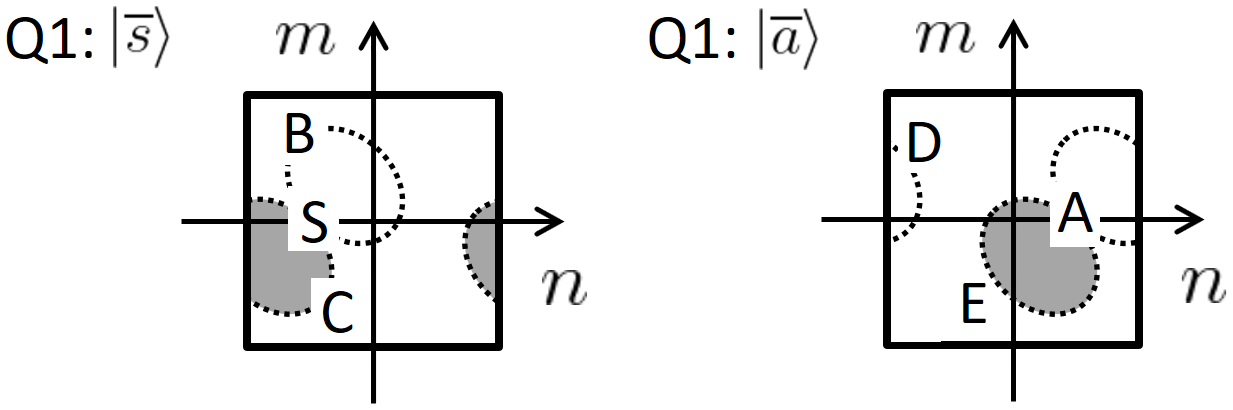
(a)

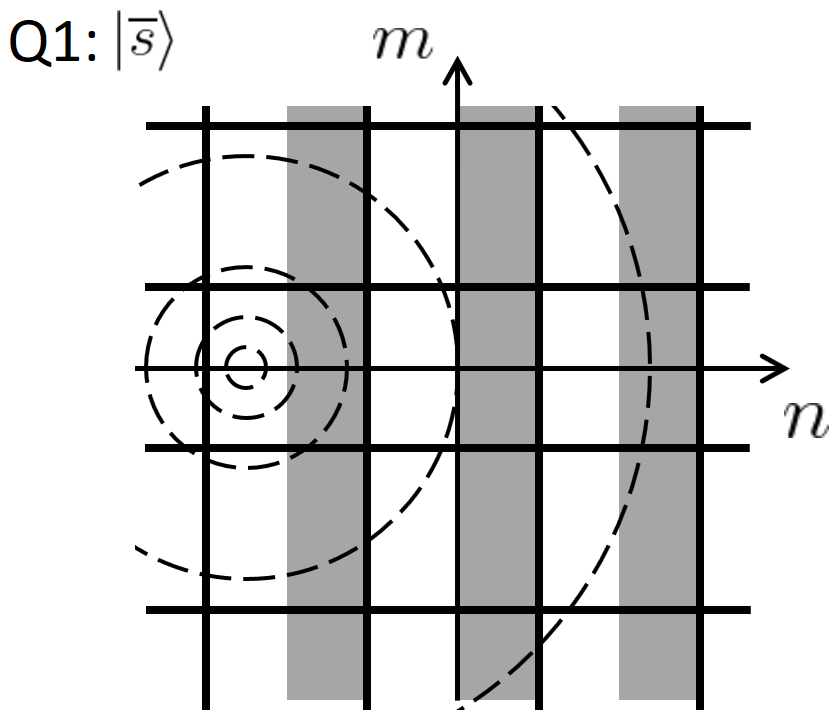
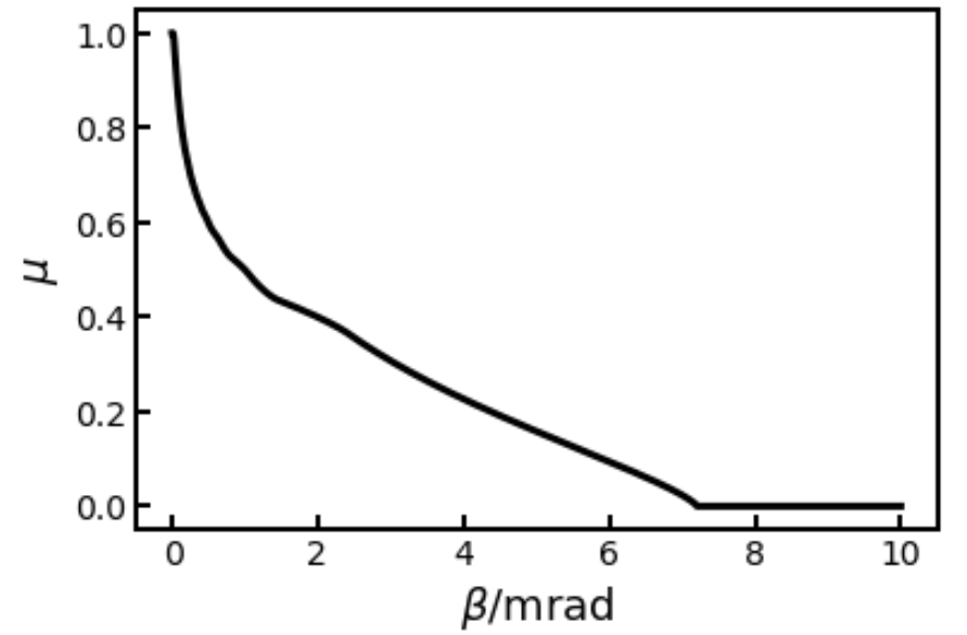
(b)(c)

Figure 2: Inelastic scattering neutralization (ISN). (a) A state appearing in inelastic scattering neutralization. We schematically show the inelastically scattered wavefunction $\Psi_{0}\left(\mathbf{k}\right)$ in the far field, which is an odd function, with unknown dipole orientation $\mathbf{a}$ (here, $\mathbf{a}$ points towards the upper-right direction). The white and gray regions indicates positive and negative regions of $\Psi_{0}\left(\mathbf{k}\right)$, although such a characterization is oversimplified because the wavefront should also have the phase factor $e^{-i\mathbf{q}\cdot\mathbf{r}_{0}}$ that represents tilt. As is the case with elastic scattering, the amplitudes at B and C, or D and E, are the negative of complex conjugate (NCC) to each other. This helps to generate $\eta\in\mathbb{R}$. (b) An averaged intensity map of inelastically scattered electron waves in the far field. This is one branch of the far field wherein Q1 state is $|\overline{s}\rangle$. Although the far field has a finite area (call it a cell) with the periodic boundary condition (PBC), here it is shown in a expanded way. The intensity of inelastically scattered electron wave, which is averaged over all dipole orientations $\mathbf{a}$, is shown in dashed circles. Although this intensity pattern is repeated due to PBC, only the one originating from the point S of a single cell is shown for clarity. The white regions correspond to the set $\mathcal{S}$ described in the text, while the gray regions correspond to $\mathcal{A}$. If one focuses on an area of either $\mathcal{S}$ or $\mathcal{A}$ type in a particular cell, then one should see that the wave intensity in that area comes from waves originating from many different cells. Subsequently, waves in $\mathcal{M}_{s}$ and $\mathcal{M}_{a}$ regions, respectively, are mixed up within these regions in the cell during the split inverse FT. Equations (122, 124) express incoherent addition of these waves. (c) This plot shows how $\mu\approx\left|\eta\right|$, which quantifies nonideality of ISN, changes with $\beta=\frac{\lambda}{2\sigma}$, where $\sigma$ is the resolution of interest. Things get better at higher resolution.

Indeed, $e_{n,m}=\psi_{0}\left(\mathbf{r}_{n,m}-\mathbf{r}_{0}\right)$ is pure imaginary. Equation (75), combined with

$$\psi_{0}\left(\mathbf{r}\right)=\mathcal{F}_{C}^{-1}\left\{\Psi_{0}\left(\mathbf{k}\right)\right\}=\int\Psi_{0}\left(\mathbf{k}\right)e^{i\mathbf{k}\cdot\mathbf{r}}\frac{d^{2}\mathbf{k}}{\left(2\pi\right)^{2}}$$ (87)

shows that

$$\psi_{0}\left(\mathbf{r}\right)^{*}=\int\Psi_{0}\left(\mathbf{k}\right)e^{-i\mathbf{k}\cdot\mathbf{r}}\frac{d^{2}\mathbf{k}}{\left(2\pi\right)^{2}}=\int\Psi_{0}\left(-\mathbf{k}\right)e^{i\mathbf{k}\cdot\mathbf{r}}\frac{d^{2}\mathbf{k}}{\left(2\pi\right)^{2}}$$

$$=-\int\Psi_{0}\left(\mathbf{k}\right)e^{i\mathbf{k}\cdot\mathbf{r}}\frac{d^{2}\mathbf{k}}{\left(2\pi\right)^{2}}=-\psi_{0}\left(\mathbf{r}\right).$$ (88)

Hence we obtain $e_{n,m}^{*}=-e_{n,m}$.

Now we exhibit the symmetry relations. Since exactly the same relations hold both for $E_{n,m}^{\left(s\right)}$ and $E_{n,m}^{\left(a\right)}$, we write these generically as $E_{n,m}$. These are

$$E_{\frac{M}{4}+a,b}=-E_{\frac{M}{4}-a,-b}^{*},$$ (89)

and

$$E_{-\frac{M}{4}+a,b}=-E_{-\frac{M}{4}-a,-b}^{*}.$$ (90)

These relations are straightforwardly obtained from Eqs. (85, 86) and the relation $e_{n,m}^{*}=-e_{n,m}$. Equations (89, 90) are crucial for keeping certain quantities real in later steps.

Figure 2 (a) shows the state of the system at this point. (See also the explanations of Fig. 1 for information about how to view the figure.) The symmetry relations make the quantum amplitudes at B and C, or those of D and E, NCC of each other. The dumbbell structure symbolically illustrates the “dipole” nature of $\Psi_{0}\left(\mathbf{k}\right)$.

IV.4 The randomization step

To strengthen later assumptions described in Sec. IV.6, here we “randomize” the coefficients $E_{n,m}^{\left(s\right)}$ and $E_{n,m}^{\left(a\right)}$. Again, we denote them collectively as $E_{n,m}$ because it can equally be taken as $E_{n,m}^{\left(s\right)}$ or $E_{n,m}^{\left(a\right)}$. This is the randomization step. Let a set of real values be $\Xi_{n,m}$, which satisfy

$$\Xi_{n+M,m}=\Xi_{n,m+M}=\Xi_{n,m},$$ (91)

$$\Xi_{\frac{M}{4}+n,m}=-\Xi_{\frac{M}{4}-n,-m}.$$ (92)

When not constrained by Eqs. (91, 92), $\Xi_{n,m}$ are chosen at random from $[0,\,2\pi)$. From these relations, one finds $\Xi_{\frac{M}{4}+n,m}=-\Xi_{-\frac{3M}{4}-n,-m}$, and then obtain, by replacing $n$ with $n-\frac{M}{2}$,

$$\Xi_{-\frac{M}{4}+n,m}=-\Xi_{-\frac{M}{4}-n,-m}.$$ (93)

One can verify that the replacement of $E_{n,m}$ with $E_{n,m}e^{i\Xi_{n,m}}$, which constitutes the randomization step, does not violate the symmetry relations.

IV.5 The split inverse Fourier transform

We show that application of split inverse QFT on $E_{n,m}$, after the randomization step, yields $g_{n,m}$ that is purely imaginary, because of the symmetry relations. By Eq. (35), we have

$$g_{\tilde{n},m}^{L}=\frac{\sqrt{2}}{M}\sum_{\left(r,s\right)\in\mathcal{M}_{s}}E_{r,s}^{\left(s\right)}e^{-2\pi i\frac{2\left(r+\frac{M}{4}\right)\tilde{n}+sm}{M}}$$

$$=\frac{\sqrt{2}}{M}\sum_{\left(r,s\right)\in\mathcal{M}_{c}}E_{r-\frac{M}{4},s}^{\left(s\right)}e^{-2\pi i\frac{2r\tilde{n}+sm}{M}},$$ (94)

and by Eq. (36) we obtain

$$g_{\tilde{n},m}^{H}=\frac{\sqrt{2}}{M}\sum_{\left(r,s\right)\in\mathcal{M}_{a}}E_{r,s}^{\left(s\right)}e^{-2\pi i\frac{2\left(r-\frac{M}{4}\right)\tilde{n}+sm}{M}}$$

$$=\frac{\sqrt{2}}{M}\sum_{\left(r,s\right)\in\mathcal{M}_{c}}E_{r+\frac{M}{4},s}^{\left(s\right)}e^{-2\pi i\frac{2r\tilde{n}+sm}{M}}.$$ (95)

Superscripts L, H denote “low-pass filtered” and “high-pass filtered”, respectively, in a similar way with the elastic scattering case. Replacement of $E_{r,s}^{\left(s\right)}$ with $E_{r,s}^{\left(a\right)}$ results in swapping of $g_{\tilde{n},m}^{H}$ and $g_{\tilde{n},m}^{L}$, as in

$$g_{\tilde{n},m}^{H}=\frac{\sqrt{2}}{M}\sum_{\left(r,s\right)\in\mathcal{M}_{s}}E_{r,s}^{\left(a\right)}e^{-2\pi i\frac{2\left(r+\frac{M}{4}\right)\tilde{n}+sm}{M}}$$ (96)

and

$$g_{\tilde{n},m}^{L}=\frac{\sqrt{2}}{M}\sum_{\left(r,s\right)\in\mathcal{M}_{a}}E_{r,s}^{\left(a\right)}e^{-2\pi i\frac{2\left(r-\frac{M}{4}\right)\tilde{n}+sm}{M}}.$$ (97)

Next, we take complex conjugation of $g_{\tilde{n},m}^{L}$:

$$\left(g_{\tilde{n},m}^{L}\right)^{*}=\frac{\sqrt{2}}{M}\sum_{\left(r,s\right)\in\mathcal{M}_{c}}E_{r-\frac{M}{4},s}^{*}e^{2\pi i\frac{2r\tilde{n}+sm}{M}}$$

$$=-\frac{\sqrt{2}}{M}\sum_{\left(r,s\right)\in\mathcal{M}_{c}}E_{-\frac{M}{4}-r,-s}e^{2\pi i\frac{2r\tilde{n}+sm}{M}}$$

$$=-\frac{\sqrt{2}}{M}\sum_{\left(r^{\prime},s^{\prime}\right)\in\mathcal{M}_{c}}E_{-\frac{M}{4}+r^{\prime},s^{\prime}}e^{-2\pi i\frac{2r^{\prime}\tilde{n}+s^{\prime}m}{M}}=-g_{\tilde{n},m}^{L},$$ (98)

where $\left(r,s\right)=\left(-r^{\prime},-s^{\prime}\right)$. Following similar steps, we obtain $\left(g_{\tilde{n},m}^{H}\right)^{*}=-g_{\tilde{n},m}^{H}$. Hence, for both low-pass and high-pass filtered versions, $g_{\tilde{n},m}$ is purely imaginary. Define $h_{\tilde{n},m}\in\mathbb{R}$ that satisfy $g_{\tilde{n},m}=ih_{\tilde{n},m}$.

Thus, we obtain Eqs. (71, 72) as resultant states after performing split inverse FT if $c=0$. We obtain

$$|a_{4}\rangle=\frac{i}{M}\sum_{\left(\tilde{n},m\right)\in\mathcal{M}_{c}}h_{\tilde{n},m}^{L}|\tilde{n},m\rangle$$ (99)

and

$$|s_{4}\rangle=\frac{i}{M}\sum_{\left(\tilde{n},m\right)\in\mathcal{M}_{c}}h_{\tilde{n},m}^{H}|\tilde{n},m\rangle$$ (100)

if $c=1$.

IV.6 Estimating $\left|\eta\right|$ that quantifies nonideality

Next, we estimate the parameter $\eta$ that appeared, following Eq. (74). We begin with a heuristic discussion. Consider Eq. (85) givng $E_{n,m}^{\left(s\right)}$. This is FT of $e_{n,m}$, whose center is placed at $\left(n,m\right)=\left(-\frac{M}{4},0\right)$. On the other hand, $e_{n,m}=\psi_{0}\left(\mathbf{r}_{n,m}-\mathbf{r}_{0}\right)$ and hence its FT is essentially $\Psi_{0}\left(\mathbf{k}\right)e^{-i\mathbf{k}\cdot\mathbf{r}_{0}}$. More precisely, the correspondence before the randomization step is

$$E_{n,m}^{\left(s\right)}\approx F\Psi_{1}\left(\mathbf{k}_{-n-\frac{M}{4},-m}\right)$$ (101)

where $\mathbf{k}_{n,m}=k_{\mathrm{min}}\left(n\hat{\mathbf{i}}+m\hat{\mathbf{j}}\right)$ and $F$ is a proportionality constant. The negative signs are a consequence of the unfortunate difference of convention between continuous and discrete FT.

Since $\Psi_{0}\left(\mathbf{k}\right)$ is large only when $\mathbf{k}$ is close to zero, $E_{n,m}^{\left(s\right)}$ clearly is large at around $n\approx-\frac{M}{4},\,m\approx 0$. By a similar argument, we find that $E_{n,m}^{\left(a\right)}$ is large near $n\approx\frac{M}{4},\,m\approx 0$. Since split inverse FT is performed separately in regions $\mathcal{M}_{s}$ and $\mathcal{M}_{a}$, $\left|h_{\tilde{n},m}^{L}\right|$ tends to be larger than $\left|h_{\tilde{n},m}^{H}\right|$.

We present estimation of the magnitude of $\left|\eta\right|$, which we believe is reasonably accurate and conceptually transparent. To make this problem tractable, first we make a quite reasonable assumption that $\left|h_{n,m}^{L}\right|>\left|h_{n,m}^{H}\right|$ mostly holds. Hence we obtain

$$\left|\eta\right|=\sum_{\left(\tilde{n},m\right)\in\mathcal{M}_{c}}p_{\tilde{n},m}\left|\frac{h_{\tilde{n},m}^{H}}{h_{\tilde{n},m}^{L}}\right|,$$ (102)

where

$$p_{\tilde{n},m}\propto\left|h_{\tilde{n},m}^{L}+i\alpha h_{\tilde{n},m}^{H}\right|^{2}+\left|h_{\tilde{n},m}^{L}+i\alpha h_{\tilde{n},m}^{H}\right|^{2}$$

$$\approx\left|h_{\tilde{n},m}^{L}\right|^{2}+\left|h_{\tilde{n},m}^{H}\right|^{2}$$ (103)

Second, note that the randomization step described above made all pixels “equal”, in the sense that all spatial frequency components, which are sinusoidal, are randomly shifted in the real space and hence there is no special location in the real space. This encourages us to use an approximation

$$p_{\tilde{n},m}=\frac{2}{M^{2}}.$$ (104)

Third, we make a standard approximation that root-mean-square roughly equals the mean of absolute values, i.e.,

$$\left|\eta\right|\approx\sqrt{\frac{2}{M^{2}}\sum_{\left(\tilde{n},m\right)\in\mathcal{M}_{c}}\left(\frac{h_{\tilde{n},m}^{H}}{h_{\tilde{n},m}^{L}}\right)^{2}}.$$ (105)

At this point, we make a brief, purely mathematical, digression to investigate whether the mean of ratios can be replaced by the ratio of means. More specifically, let $a_{n},\,b_{n}$ be series, where $n=1,2,\cdots,N$. We assume that $a_{n}\ll b_{n}$ for all $n$. Hence we write $a_{n}=\varepsilon_{n}b_{n}$, where $\varepsilon_{n}\ll 1$. Write this series $\varepsilon_{n}=\varepsilon+\delta_{n}$, where $\sum_{n}\delta_{n}=0$. Also write $b_{n}=b+d_{n}$, where $\sum_{n}d_{n}=0$. Consider the mean of ratios

$$\frac{1}{N}\sum_{n}\frac{a_{n}}{b_{n}}=\frac{1}{N}\sum_{n}\varepsilon_{n}=\varepsilon+\frac{1}{N}\sum_{n}\delta_{n}=\varepsilon.$$ (106)

On the other hand, the ratio of means is

$$\frac{\frac{1}{N}\sum_{n}a_{n}}{\frac{1}{N}\sum_{n}b_{n}}=\frac{\sum_{n}\varepsilon_{n}b_{n}}{\sum_{n}b_{n}}$$

$$=\frac{\varepsilon\sum_{n}b_{n}+\sum_{n}\delta_{n}b_{n}}{\sum_{n}b_{n}}=\varepsilon+\frac{\sum_{n}\delta_{n}b_{n}}{\sum_{n}b_{n}}$$

$$=\varepsilon+\frac{b\sum_{n}\delta_{n}+\sum_{n}\delta_{n}d_{n}}{\sum_{n}b_{n}}=\varepsilon+\frac{\sum_{n}\delta_{n}d_{n}}{Nb}.$$ (107)

Comparing these, we conclude that the mean of ratio is close to the ratio of means if two series $\delta_{n},\,d_{n}$ are only weakly correlated.

Fourth, going back to the main line of reasoning, we assume that the conditions for the above “theorem” are met with $\left(h_{\tilde{n},m}^{H}\right)^{2}$ and $\left(h_{\tilde{n},m}^{L}\right)^{2}$, where the former is identified with $a_{n}$ while the latter corresponds to $b_{n}$. Then, we may use what we have just shown to obtain, from Eq. (105),

$$\left|\eta\right|\approx\sqrt{\frac{\sum_{\left(\tilde{n},m\right)\in\mathcal{M}_{c}}\left(h_{\tilde{n},m}^{H}\right)^{2}}{\sum_{\left(\tilde{n},m\right)\in\mathcal{M}_{c}}\left(h_{\tilde{n},m}^{L}\right)^{2}}}.$$ (108)

Application of Parseval’s theorem to Eq. (94) yields

$$\sum_{\left(\tilde{n},m\right)\in\mathcal{M}_{c}}\left(h_{\tilde{n},m}^{L}\right)^{2}=\sum_{\left(n,m\right)\in\mathcal{M}_{s}}\left|E_{n,m}^{\left(s\right)}\right|^{2}.$$ (109)

From Eq. (96), we also obtain

$$\sum_{\left(\tilde{n},m\right)\in\mathcal{M}_{c}}\left(h_{\tilde{n},m}^{H}\right)^{2}=\sum_{\left(n,m\right)\in\mathcal{M}_{s}}\left|E_{n,m}^{\left(a\right)}\right|^{2}.$$ (110)

On the other hand, Eq. (85) says, for all $\left(r,s\right)\in\mathbb{Z}^{2}$,

$$E_{n,m}^{\left(s\right)}=E_{n+Mr,m+Ms}^{\left(s\right)}.$$ (111)

We incorporate this periodicity in Eq. (101) to obtain more accurate expression:

$$E_{n,m}^{\left(s\right)}\approx F\sum_{\left(r,s\right)\in\mathbb{Z}^{2}}\Psi_{1}\left(\mathbf{k}_{-n-M\left(r+\frac{1}{4}\right),-m-Ms}\right)e^{i\Xi_{n,m}}.$$ (112)

At this point, we make further approximation that the phase factor in this equation is totally random. The presence of randomization step described in Sec. IV.4 prompts us to accept this assumption. We use a mathematical identity

$$\left|\sum_{k}a_{k}e^{i\theta_{k}}\right|^{2}=\sum_{k}\left|a_{k}\right|^{2}+2\sum_{k\neq l}a_{k}a_{l}\cos\left(\theta_{k}-\theta_{l}\right),$$ (113)

where $a_{k}\in\mathbb{R}$ and the second term averages to zero when $\theta_{k}$ are all random. We obtain

$$\left|E_{n,m}^{\left(s\right)}\right|^{2}\approx F^{2}\left\{\sum_{\left(r,s\right)\in\mathbb{Z}^{2}}\left|\Psi_{1}\left(\mathbf{k}_{-n-M\left(r+\frac{1}{4}\right),-m-Ms}\right)\right|^{2}\right\}.$$ (114)

Recall that $\Psi_{0}\left(\mathbf{k}\right)$, mentioned in Eq. (75), includes a particular direction $\mathbf{a}$ of the dipole. This direction should be regarded random and our analysis should be averaged over the direction of $\mathbf{a}$. We assume that such averaging can be done here, rather than at the final stage of computing $\left|\eta\right|$ without introducing significant error. Equation (75) can be expressed as

$$\Psi_{0}\left(\mathbf{k}\right)=\begin{cases}\frac{a\cos\xi}{\sqrt{\theta^{2}+\theta_{E}^{2}}}&\theta<\theta_{c}\\ 0&\theta>\theta_{c}\end{cases},$$ (115)

where $\xi$ is the angle between $\mathbf{k}$ and $\mathbf{a}$. Hence

$$\left|\Psi_{1}\left(\mathbf{k}\right)\right|^{2}=\left|\Psi_{0}\left(\mathbf{k}\right)\right|^{2}=\begin{cases}\frac{a^{2}\cos^{2}\xi}{\theta^{2}+\theta_{E}^{2}}&\theta<\theta_{c}\\ 0&\theta>\theta_{c}\end{cases}$$ (116)

To compute the average of $\cos^{2}\xi$ in $3$ dimensional space, we take the $z$-axis parallel to $\mathbf{k}$ and move $\frac{\mathbf{a}}{a}$ on the unit sphere $\mathcal{U}$. The average of $\cos^{2}\xi$ is, using obvious notations of polar coordinates,

$$\int_{\mathcal{U}}\cos^{2}\xi\frac{dS}{4\pi}=\frac{1}{2}\int_{0}^{\pi}d\xi\cos^{2}\xi\cdot\sin\xi==\frac{1}{3}.$$ (117)

Henceforth we use the averaged version $\Phi\left(\mathbf{k}\right)$ shown below, instead of $\left|\Psi_{0}\left(\mathbf{k}\right)\right|^{2}$:

$$\Phi\left(\mathbf{k}\right)=\begin{cases}\frac{a^{2}}{3}\cdot\frac{1}{\theta^{2}+\theta_{E}^{2}}&\theta<\theta_{c}\\ 0&\theta>\theta_{c}\end{cases},$$ (118)

where the factor $\frac{a^{2}}{3}$ is not important after all.

Recalling that $\mathbf{k}_{a,b}=k_{\mathrm{min}}\left(a\hat{\mathbf{i}}+b\hat{\mathbf{j}}\right)$, we approximate a sum by an integral:

$$\sum_{\left(n,m\right)\in\mathcal{M}_{s}}\left|E_{n,m}^{\left(s\right)}\right|^{2}k_{\mathrm{min}}^{2}$$

$$\approx F^{2}\sum_{\left(r,s\right)\in\mathbb{Z}^{2}}\int_{\mathcal{D}}d^{2}\mathbf{k}\Phi\left(\mathbf{k}+k_{\mathrm{max}}\left(r\hat{\mathbf{i}}+s\hat{\mathbf{j}}\right)\right),$$ (119)

where $\mathcal{D}$ denotes a region

$$\mathcal{D}=\left\{\left(k_{x,}k_{y}\right)|-\frac{k_{\mathrm{max}}}{4}<k_{x}<\frac{k_{\mathrm{max}}}{4},\,-\frac{k_{\mathrm{max}}}{2}<k_{y}<\frac{k_{\mathrm{max}}}{2}\right\},$$ (120)

where $\left(k_{x},k_{y}\right)\in\mathbb{R}^{2}$. Equivalently, one can define a region $\mathcal{S}$, which is a set of “stripes”:

$$\mathcal{S}=\bigcup_{r\in\mathbb{Z}}\left\{\left(k_{x,}k_{y}\right)|r-\frac{1}{4}<\frac{k_{x}}{k_{\mathrm{max}}}<r+\frac{1}{4}\right\},$$ (121)

to express

$$\sum_{\left(n,m\right)\in\mathcal{M}_{s}}\left|E_{n,m}^{\left(s\right)}\right|^{2}k_{\mathrm{min}}^{2}\approx F^{2}\int_{\mathcal{\mathcal{S}}}d^{2}\mathbf{k}\Phi\left(\mathbf{k}\right).$$ (122)

A similar argument on $E_{n,m}^{\left(a\right)}$ yields

$$\mathcal{A}=\bigcup_{r\in\mathbb{Z}}\left\{\left(k_{x,}k_{y}\right)|r+\frac{1}{4}<\frac{k_{x}}{k_{\mathrm{max}}}<r+\frac{3}{4}\right\},$$ (123)

and

$$\sum_{\left(n,m\right)\in\mathcal{M}_{s}}\left|E_{n,m}^{\left(a\right)}\right|^{2}k_{\mathrm{min}}^{2}\approx F^{2}\int_{\mathcal{\mathcal{A}}}d^{2}\mathbf{k}\Phi\left(\mathbf{k}\right).$$ (124)

Thus we obtain

$$\left|\eta\right|\approx\sqrt{\frac{\int_{\mathcal{\mathcal{A}}}d^{2}\mathbf{k}\Phi\left(\mathbf{k}\right)}{\int_{\mathcal{\mathcal{S}}}d^{2}\mathbf{k}\Phi\left(\mathbf{k}\right)}}.$$ (125)

We call the right hand side $\mu$ hereafter.

Figure 2 (b) is a conceptual picture relevant to the above argument, which the reader may find useful. Figure 2 (c) shows $\mu$ as a function of $\beta=\frac{\lambda}{2\sigma}$, where $\lambda=1.97\,\mathrm{pm}$ is the wavelength of $300\,\mathrm{keV}$ electrons.

IV.7 Multiple inelastic scattering in a single round of quantum measurement

Consider the effect of multiple inelastic scattering. Suppose that they occurred $w$ times. We first note that, in the above entire reasoning, the parameter $\alpha$ in Eq. (47) could have been any complex number. We explicitly write $\alpha=\rho+i\kappa$, and the state before inelastic scattering is

$$|\overline{s}\rangle+\left(i\rho-\kappa\right)|\overline{a}\rangle.$$ (126)

After inelastic scattering, we obtain

$$\left(|\overline{s}\rangle+i\alpha|\overline{a}\rangle\right)+\eta\left(|\overline{a}\rangle+i\alpha|\overline{s}\rangle\right)$$

$$=\left(1+i\rho\eta-\kappa\eta\right)|\overline{s}\rangle+\left(i\rho-\kappa+\eta\right)|\overline{a}\rangle.$$ (127)

Assuming that $\rho\eta$ and $\kappa\eta$ are small, this state approximately equals

$$|\overline{s}\rangle+\left(i\rho-\kappa+\eta\right)|\overline{a}\rangle.$$ (128)

This shows that the effect of inelastic scattering additively accumulates. In other words, after $n$ inelastic scattering, each with associated $\eta$ parameter $\eta_{i},\,i=1,2,\cdots,n$, we obtain a Q1 state of a form

$$|\overline{s}\rangle+\left(i\rho+\sum_{i=1}^{n}\eta_{i}\right)|\overline{a}\rangle.$$ (129)

To develop a rough picture, assume that all $\eta_{i}$ have the same absolute value $\mu>0$ derived in Eq. (125), but their signs are random. Then $\sum_{i=1}^{w}\eta_{i}$ represents random walk on the real line, which results in

$$\left|\sum_{i=1}^{w}\eta_{i}\right|\approx\sqrt{w}\mu.$$ (130)

IV.8 Estimating the final outcome of imaging

Finally, we consider how the accumulated error $\sqrt{w}\mu$ affects our measurement. Consider a general qubit state

$$|\overline{\psi}\rangle=e^{-i\frac{\varphi}{2}}\cos\frac{\theta}{2}|\overline{0}\rangle+e^{i\frac{\varphi}{2}}\sin\frac{\theta}{2}|\overline{1}\rangle,$$ (131)

where $\theta,\,\varphi$ are latitude and longitude on the Bloch sphere, respectively. Comparing with Eq. (129, 130), we find that $\theta,\,\varphi$ correspond to $\rho,\,\sqrt{w}\mu$ as

$$\varphi=-2\rho,$$ (132)

$$\theta=\frac{\pi}{2}-2\sqrt{w}\mu=\frac{\pi}{2}-\Theta,$$ (133)

where we defined $\Theta$ to indicate the angular deviation from the ideal great circle on the Bloch sphere, which passes the states $|\overline{s}\rangle,\,|\overline{a}\rangle,\,|\overline{\uparrow}\rangle,\,|\overline{\downarrow}\rangle$. Hence $|\overline{\psi}\rangle$ expressed in terms of $\theta,\,\varphi$ is

$$|\overline{\psi}\rangle=e^{i\rho}\cos\left(\frac{\pi}{4}-\frac{\Theta}{2}\right)|\overline{0}\rangle+e^{-i\rho}\sin\left(\frac{\pi}{4}-\frac{\Theta}{2}\right)|\overline{1}\rangle.$$ (134)

Using the basis state $|\overline{\uparrow}\rangle,\,|\overline{\downarrow}\rangle$, we obtain (multiplying an overall phase factor $e^{i\frac{\varphi}{2}}$)

$$|\overline{\psi}\rangle=C_{\uparrow}|\overline{\uparrow}\rangle+C_{\downarrow}|\overline{\downarrow}\rangle,$$ (135)

where

$$C_{\uparrow}=\frac{\cos\frac{\theta}{2}-ie^{i\varphi}\sin\frac{\theta}{2}}{\sqrt{2}},$$ (136)

$$C_{\downarrow}=\frac{\cos\frac{\theta}{2}+ie^{i\varphi}\sin\frac{\theta}{2}}{\sqrt{2}}$$ (137)

and hence

$$p_{\uparrow}=\left|C_{\uparrow}\right|^{2}=\frac{1+\sin\theta\sin\varphi}{2}$$

$$=\frac{1-\cos\Theta\sin\left(2\rho\right)}{2}\approx\frac{1}{2}-\rho\cos\Theta,$$ (138)

$$p_{\downarrow}=\left|C_{\downarrow}\right|^{2}\approx\frac{1}{2}+\rho\cos\Theta.$$ (139)

Hence the signal we want to detect, $\rho$, weakens by the factor $\cos\Theta$.

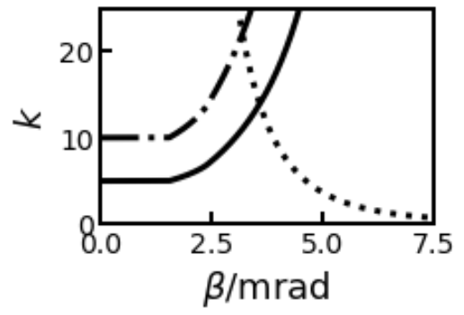
Figure 3: The optimal repetition number $k$, enabled by inelastic scattering neutralization, is plotted against $\beta=\lambda/2\sigma$, where $\sigma$ is resolution of interest. For example, $\beta=2\,\mathrm{mrad}$ corresponds to $\sigma=0.5\,\mathrm{nm}$. The phase resolution is improved by $\approx 0.65\sqrt{k}$. The dash-dotted curve and the solid curve correspond to $k_{\mathrm{opt}}$ defined in the main text for $\Lambda/t=10$ and $5$, which roughly correspond to the specimen thickness of $t\approx 30\,\mathrm{nm}$ and $60\,\mathrm{nm}$, respectively. On the other hand, radiation damage governs the allowed number of electrons $N_{\mathrm{sq}}$ (the dotted curve) and the actual repetition number $k$ should equal $\min\left\{k_{\mathrm{opt}},\,N_{\mathrm{sq}}\right\}$.

Next, we consider improvement in terms of signal-to-noise ratio (SNR). A single round of quantum measurement comprises transmission of $k$ electrons through the specimen. The number of inelastic scattering events in a single round of quantum measurement is, on average

$$w=\frac{kt}{\Lambda},$$ (140)

where $k$ is the repetition number, $t$ is the specimen thickness, and $\Lambda$ is the inelastic mean free path. Let half the phase difference between specimen areas $0$ and $1$, where the electron states $|\overline{0}\rangle,\,|\overline{1}\rangle$ are respectively focused, that we want to measure, be $\overline{\theta}$. The accumulated phase after a single round of quantum measurement, weakened by inelastic scattering events, is

$$k\overline{\theta}\cos\Theta=k\overline{\theta}\cos\left(2\sqrt{w}\mu\right)=k\overline{\theta}\cos\left(2\sqrt{\frac{kt}{\Lambda}}\mu\right).$$ (141)

We use $N$ electrons and try this $\frac{N}{k}$ times. In the language of binomial distribution $B\left(n,p\right)$, where $n=\frac{N}{k}$ and $p=\frac{1}{2}+k\overline{\theta}\cos\Theta$ in the present case, the mean is $np=\frac{N}{2k}+N\overline{\theta}\cos\Theta$ and the variance is $np\left(1-p\right)\approx\frac{N}{4k}$. We divide the signal

$$N\overline{\theta}\cos\Theta$$ (142)

by noise, which is square root of the variance

$$\frac{1}{2}\sqrt{\frac{N}{k}}.$$ (143)

We want to find the optimal repetition number $k_{2}$, which maximizes SNR. To find $k_{2}$, we may consider a quantity that is square of the ratio of Eq. (142) to Eq. (143):

$$4Nk\overline{\theta}^{2}\cos^{2}\Theta\propto k\cos^{2}\left(2\sqrt{\frac{kt}{\Lambda}}\mu\right)=F\left(k\right).$$ (144)

Then, we should get $\frac{dF\left(k\right)}{dk}=0$ at $k=k_{2}$. We find a condition

$$\frac{dF\left(k\right)}{dk}=\cos^{2}\xi-\xi\cos\xi\sin\xi=0,$$

or equivalently

$$\frac{1}{\xi}=\tan\xi,$$ (145)

in terms of

$$\xi=2\sqrt{\frac{kt}{\Lambda}}\mu.$$ (146)

Numerical solution to this equation turns out to be $\xi=0.86$ and we further obtain $\xi^{2}=0.74$. Thus we get

$$k_{2}=\frac{\xi^{2}}{4\mu^{2}}\frac{\Lambda}{t}\approx\frac{0.74}{4\mu^{2}}\frac{\Lambda}{t}$$ (147)

and improvement of S/N is

$$\sqrt{k_{2}}\cos\left(2\sqrt{\frac{k_{2}t}{\Lambda}}\mu\right)=\sqrt{k_{2}}\cos\xi.$$ (148)

When $\mu^{2}$ is large at low resolution, we may as well not perform inelastic scattering neutralization. In the absence of inelastic scattering neutralization, the optimal $k$ is $k_{1}=\Lambda/t$ and improvement of S/N ratio is $\sqrt{k_{1}/e}=\sqrt{\Lambda/et}$ as shown in Eq. (1). These results show advantage of inelastic scattering neutraliztion because we can use a larger $k_{2}$ than $k_{1}$ when $\mu^{2}$ is small, as shown in Eq. (147). Otherwise we should employ $k_{1}$. In this case, S/N ratios given by Eqs. (1) and (148) turn out to be similar. Indeed, numerically, $\cos\xi\approx 0.65$ is close to $\frac{1}{\sqrt{e}}\approx 0.61$, indicating that Eq. (148) is not too bad with a moderately large $\mu^{2}$, although our calculations implicitly assumed a small $\mu^{2}$. See Sec. V for information about the repetition number $k$ that the experimenter should choose at a given SF.

Since it is better not to use ISN when $\mu^{2}$ is too large, we define $k_{\mathrm{opt}}=\max\left\{k_{2},k_{1}\right\}$. On the other hand, $k$ cannot exceed the dose limit $N_{\mathrm{sq}}$ of Eq. (14). Figure 3 shows how $k_{\mathrm{opt}}$ and $N_{\mathrm{sq}}$ depend on $\beta=\lambda/2\sigma$.

V Expected improvement: A simulation study

To visually assess the improvement afforded by ISN, we simulate imaging of the Marburg virus VP35 domain molecule 5TOI (24). Figure 4 shows the result. The noiseless map of phase shift shown in Fig. 4 (a) is produced by multislice simulation as described in Appendix D. Figures 4 (b)-(f) are addition of the phase map and noise. Figure 4 (b) shows the case without quantum advantage. (However, SF-dependent electron dose control mentioned in Sec. III.1 is employed and hence this is not conventional TEM imaging.) Figures 4 (c), (d) shows simulated images with and without ISN for a thin ($\approx 30\,\mathrm{nm}$) specimen, whereas Figs. 4 (e), (f) shows corresponding images for a relatively thick ($\approx 60\,\mathrm{nm}$) specimen. For simplicity, we assume that energy loss $E$ is always $20\,\mathrm{eV}$ Leapman_Sun (25). All computations are performed on $240\times 240$ pixels image data, with each square pixel having the side length $l=0.05\,\mathrm{nm}$. We label each pixel with a pair of integers $\left(n,\,m\right)$, each of which ranges from $-120$ to $119$.

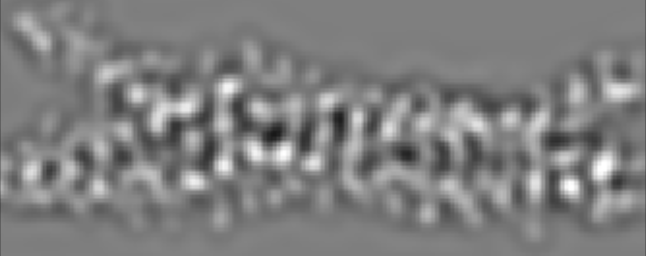
(a) (b) (c) (d)

(e) (f)

Figure 4: Simulated images of the Marburg virus VP35 domain molecule 5TOI (24). (a) A band-pass filtered phase map. (b) Imaging without quantum enhancement, i.e. the repetition number $k=1$. (c) QEM imaging without inelastic scattering neutralization (ISN), wherein $k_{1}=\Lambda/t=10$, roughly corresponding to a specimen thickness $t\approx 30\,\mathrm{nm}$. (d) QEM imaging with ISN. The repetition number is $\tilde{k}_{2}$, where $\Lambda/t=10$. (e) QEM imaging without ISN, wherein $\Lambda/t=5$ (i.e. specimen thickness $t\approx 60\,\mathrm{nm}$). (f) QEM imaging with ISN, wherein $\Lambda/t=5$. The horizontal length of all images is $10\,\mathrm{nm}$.

In what follows, we describe the procedure to generate noise in each case. Typically, although not always, many rounds of quantum measurements, each involving $k$ electron passing events, are performed for each pixel. Hence we expect the noise to be approximately gaussian, which approximates the binomial distribution. In all three imaging methods — i.e. TEM with no quantum enhancement but with SF-dependent dose control, “conventional QEM”, and QEM with ISN — the amount of noise depends on

$$\beta=\frac{q}{k_{z}}=\frac{\pi}{\sigma k_{z}}=\frac{\lambda}{2\sigma},$$ (149)

where $k_{z}$ is the wave number along the optical axis, and $\lambda=2\pi/k_{z}\approx 1.97\,\mathrm{pm}$ is the wavelength of $300\,\mathrm{keV}$ electrons. Equation (149) is valid insofar as the vector $\mathbf{q}$ may be regarded as being perpendicular to the optical axis.

Specific steps are the following. First, we generate real-valued, independent gaussian noise, with zero mean and unit variance, in each pixel on the image plane. Second, we perform fast Fourier transform (FFT) to obtain the noise in the diffraction plane, which results in a complex-valued map. The pixel $\left(0,119\right)$ in the map, for example, corresponds to a scattering angle

$$\beta\approx\sin\beta=\frac{\lambda}{2l}=\frac{1.97\,\mathrm{pm}}{2\times 0.05\,\mathrm{nm}}\times\frac{119}{120}=19.5\,\mathrm{mrad}.$$ (150)

Third, to the map on the diffraction plane we multiply a function that describes the $q$-dependent amplitude of noise. For the “classical” case of Fig. 4 (b), we multiply the standard deviation of shot noise

$$\frac{1}{\sqrt{N_{\mathrm{sq}}}}=\frac{1}{\sqrt{F_{\mathrm{sq}}A}}=\sqrt{\frac{Rq^{4}}{32\pi^{5}\zeta}}=\sqrt{\frac{R}{32\pi^{5}\zeta}}\frac{q^{2}}{k_{z}^{2}}k_{z}^{2}$$

$$=\frac{10^{-6}}{\lambda^{2}}\sqrt{\frac{R}{2\pi\zeta}}\left(\frac{\beta}{\mathrm{mrad}}\right)^{2}=\frac{\left(\beta/\mathrm{mrad}\right)^{2}}{186},$$ (151)

where $\zeta=0.255$ as described in Sec. III.1. Uncertainties associated with parameters such as $R,\,\zeta$ do not warrant the precision appearing in the numerical value $186$, but we use this value in the simulation anyway. Equation (151) overestimates noise when $N_{\mathrm{sq}}<1$, where we do not perform measurement and hence there is no noise (and no signal). However, computed images in Fig. 4 is bandpass-filtered anyway and hence this particular artefact does not matter.

The images shown in Figs. 4 (c)-(f) have smaller noise than Eq. (151) indicates, because of quantum advantage. To discuss degrees of noise reduction, using $k_{1},k_{\mathrm{opt}}$ and $\xi$ defined in Sec. IV.8, we define

$$\tilde{k}_{1}=\max\left\{\min\left\{k_{1},N_{\mathrm{sq}}\right\},e\right\},$$ (152)

and

$$\tilde{k}_{2}=\max\left\{\min\left\{k_{\mathrm{opt}},N_{\mathrm{sq}}\right\},\cos^{-2}\xi\right\}.$$ (153)

We obtain $\cos^{-2}\xi=2.35$ from Eq. (145). Hence Eq. (153) can more specifically be written as, noting $\sqrt{0.74/4}=0.43$,

$$\tilde{k}_{2}=\max\left\{\min\left\{k_{1}\max\left\{\left(\frac{0.43}{\mu}\right)^{2},1\right\},N_{\mathrm{sq}}\right\},2.35\right\}.$$ (154)

Remark: Figure 2 (c), along with Fig. 3, clearly show that the resolution, at which $N_{\mathrm{sq}}=2.35$, is much higher than another resolution, where $\mu=0.43$ holds.

For the QEM cases, we multiply factors of noise reduction compared to the classical case of Eq. (151). They are, first,

$$\sqrt{\frac{e}{\tilde{k}_{1}}}.$$ (155)

for QEM without ISN and second,

$$\frac{1}{\sqrt{\tilde{k}_{2}}\cos\xi}$$ (156)

for QEM with ISN.

Here we elaborate on Eq. (152) somewhat. Since the noise reduction factor compared to classical imaging is $\sqrt{\frac{e}{\tilde{k}_{1}}}$, there is no point in employing $\tilde{k}_{1}$ less than $e$. One would simply perform classical measurement in this case. The outermost “max” function in Eq. (152) ensures that we get at least the classical performance. Otherwise we would use $k_{1}$ as the repetition number, unless $k_{1}$ exceeds the dose limit $N_{\mathrm{sq}}$. In the latter case, we take $N_{\mathrm{sq}}$ as the repetition number of the quantum measurement.

The idea behind Eq. (154) for $\tilde{k}_{2}$ is similar. Once again, the outermost “max” function ensures the classical performance in the worst case. The “min” function in it ensures that we do not exceed the dose limit $N_{\mathrm{sq}}$. The innermost “max” function makes sure that ISN is employed only when it is advantageous, compared to “conventional” QEM, to do so.

Fourth and finally, we apply inverse FFT to obtain spatial-frequency-weighted noise patterns. The result should mathematically be real, but the real part should be taken in actual numerical computation. The resultant noise patterns are simply added to the phase map, i.e. $\theta\left(x,y\right)$ of the exit wave $1+i\theta\left(x,y\right)$ (shown in Fig. 4 (a)) to obtain Figs. 4 (b)-(f).

A bandpass filter is applied to images because the improvement by ISN is mainly at high resolution and visually rather subtle, requiring removal of large low resolution components. Thus all six images are filtered by multiplying a function $e^{-\beta^{2}/2\beta_{H}^{2}}\left(1-e^{-\beta^{2}/2\beta_{L}^{2}}\right)$ in the $\beta_{x}\beta_{y}$-space, where $\beta^{2}=\beta_{x}^{2}+\beta_{y}^{2}$, $\beta_{L}=2\,\mathrm{mrad}$ and $\beta_{H}=3.5\,\mathrm{mrad}$. The contrast of all images in Fig. 4 (a)-(f) are adjusted in the following way. Given a numerical array representing an image, the mean $\bar{\mu}$ and the standard deviation $\bar{\sigma}$ are computed. The highest and the lowest brightness in each presented image are then made to correspond to the values $\bar{\mu}+5\bar{\sigma}$ and $\bar{\mu}-5\bar{\sigma}$, respectively. Finally, the images are cropped to the size of approximately $80\times 200$ pixels for presentation.

VI Conclusion

In summary, it is in principle possible to neutralize, to the extent we discussed, inelastic scattering especially at high resolution. We conjecture that this is essentially the fundamental limit of electron microscopy of beam sensitive specimens, when performing standard imaging. On the other hand, non-standard imaging, such as image verification OLF (26) among other possibilities, is worth further study.

APPENDIX A: ENTANGLEMENT ENHANCED ELECTRON MICROSCOPY: A BRIEF INTRODUCTION

In this section, we briefly review entanglement-enhanced electron microscopy eeem_cpb (11, 12, 13) for readers who are unfamiliar with the scheme. This review purposely avoids the implementation aspect of the scheme, such as the use of superconducting quantum devices. Instead, we focus on principles and therefore we take it for granted that all theoretically possible operations, such as unitary transformations, addition of an initialized ancilla qubit, and measurements on arbitrary subsystems are possible. We ignore the spin of the electron, regarding it to be decoupled from the degrees of freedom of interest. We intend to make Appendix A as self-contained as possible. As a result, there are few redundancies with the main text.

Let the electron states $|0\rangle,\,|1\rangle$ be ones that are localized on non-overlapping regions $0$ and $1$ on a biological specimen when the electron passes the specimen. Recall that the specimen may be regarded as a weak phase object in cryoEM. We want to measure the difference in phase shifts between the regions $0$ and $1$. Keep in mind that there are many electron states other than $|0\rangle,\,|1\rangle$. Define symmetric and asymmetric states as

$$|s\rangle=\frac{|0\rangle+|1\rangle}{\sqrt{2}},\;|a\rangle=\frac{|0\rangle-|1\rangle}{\sqrt{2}}.$$ (157)

Let the initial electron state be $|0\rangle$. Consider a separate $2$-state system (call it qubit Q1) with basis states $|\overline{0}\rangle,\,|\overline{1}\rangle$, where the bar indicates that the state belongs to Q1. Another set of basis states $|\overline{s}\rangle,\,|\overline{a}\rangle$ for Q1 is defined in terms of $|\overline{0}\rangle,\,|\overline{1}\rangle$ exactly as in Eq. (157). Suppose that Q1 is in the state

$$|\overline{\alpha}\rangle=\frac{e^{i\alpha}|\overline{0}\rangle+e^{-i\alpha}|\overline{1}\rangle}{\sqrt{2}},$$ (158)

for some $\alpha$, whose significance will be apparent shortly. We occasionally write a state of the combined system of an electron in a state $u$, and the qubit in a state $\overline{v}$, as

$$|u\overline{v}\rangle=|u\rangle\otimes|\overline{v}\rangle.$$ (159)

Hence we write the current state as $|0\overline{\alpha}\rangle$. Let $U$ be a unitary operation, which flips the electron state as $|0\rangle\Rightarrow|1\rangle,\,|1\rangle\Rightarrow|0\rangle$ if and only if the qubit is in the state $|\overline{1}\rangle$. (This should be realizable with a superconducting qubit eeem_cpb (11, 12, 13).) In other words,

$$\alpha|0\rangle+\beta|1\rangle\Rightarrow\beta|0\rangle+\alpha|1\rangle$$ (160)

if and only if the qubit is in the state $|\overline{1}\rangle$. In short, $U$ is the quantum controlled-NOT gate in the language of quantum information science. We apply $U$ to the electron-qubit system in the initial state $|0\overline{\alpha}\rangle$, which results in

$$\frac{e^{i\alpha}|0\overline{0}\rangle+e^{-i\alpha}|1\overline{1}\rangle}{\sqrt{2}}.$$ (161)

Upon passing the biological specimen, the two electron states $|0\rangle,\,|1\rangle$ acquire different phase shifts as

$$|0\rangle\Rightarrow e^{i\theta}|0\rangle,\;|1\rangle\Rightarrow e^{-i\theta}|1\rangle,$$ (162)

where $\theta$ is half the relative phase shift between the specimen regions $0$ and $1$, which correspond respectively to the localized electron states $|0\rangle,\,|1\rangle$. Our objective is to determine $\theta$ as precisely as possible. After the electron transmits through the specimen, the state of the entire system is

$$\frac{e^{i\left(\alpha+\theta\right)}|0\overline{0}\rangle+e^{-i\left(\alpha+\theta\right)}|1\overline{1}\rangle}{\sqrt{2}}=\frac{|s\rangle}{\sqrt{2}}\otimes\frac{e^{i\left(\alpha+\theta\right)}|\overline{0}\rangle+e^{-i\left(\alpha+\theta\right)}|\overline{1}\rangle}{\sqrt{2}}+\frac{|a\rangle}{\sqrt{2}}\otimes\frac{e^{i\left(\alpha+\theta\right)}|\overline{0}\rangle-e^{-i\left(\alpha+\theta\right)}|\overline{1}\rangle}{\sqrt{2}}.$$ (163)

Next, we measure the electron state in the basis $\left\{|s\rangle,\,|a\rangle\right\}$. If the measurement outcome indicates $|s\rangle$, then the qubit is left in the state

$$\frac{e^{i\left(\alpha+\theta\right)}|\overline{0}\rangle+e^{-i\left(\alpha+\theta\right)}|\overline{1}\rangle}{\sqrt{2}}.$$ (164)

Likewise, when the outcome indicates $|a\rangle$, then the qubit state is

$$\frac{e^{i\left(\alpha+\theta\right)}|\overline{0}\rangle-e^{-i\left(\alpha+\theta\right)}|\overline{1}\rangle}{\sqrt{2}},$$ (165)

which can readily be brought to Eq. (164) by the Pauli-Z-gate operation $|\overline{0}\rangle\Rightarrow|\overline{0}\rangle,\;|\overline{1}\rangle\Rightarrow-|\overline{1}\rangle$. Thus, the overall effect of passing an electron through the specimen is to have the qubit state evolution from Eq. (158) to Eq. (164). This means that we can start with $\alpha=0$ and repeat the process $k$ times, which means that $k$ electrons pass the specimen, to obtain the state

$$\frac{e^{ik\theta}|\overline{0}\rangle+e^{-ik\theta}|\overline{1}\rangle}{\sqrt{2}}.$$ (166)

Consequently, the small phase shift $\theta$ accumulate on Q1 $k$ times. Next, we measure this qubit state with respect to the basis states

$$|\overline{\uparrow}\rangle=\frac{|\overline{0}\rangle+i|\overline{1}\rangle}{\sqrt{2}},\,|\overline{\downarrow}\rangle=\frac{|\overline{0}\rangle-i|\overline{1}\rangle}{\sqrt{2}}.$$ (167)

Hence Eq. (166) equals

$$\frac{1}{2}\left\{e^{ik\theta}\left(|\overline{\uparrow}\rangle+|\overline{\downarrow}\rangle\right)-ie^{-ik\theta}\left(|\overline{\uparrow}\rangle-|\overline{\downarrow}\rangle\right)\right\}=\frac{e^{ik\theta}-ie^{-ik\theta}}{2}|\overline{\uparrow}\rangle+\frac{e^{ik\theta}+ie^{-ik\theta}}{2}|\overline{\downarrow}\rangle$$

$$=e^{-i\frac{\pi}{4}}\frac{e^{i\left(\frac{\pi}{4}+k\theta\right)}+e^{-i\left(\frac{\pi}{4}+k\theta\right)}}{2}|\overline{\uparrow}\rangle+e^{i\frac{\pi}{4}}\frac{e^{i\left(\frac{\pi}{4}-k\theta\right)}+e^{-i\left(\frac{\pi}{4}-k\theta\right)}}{2}|\overline{\downarrow}\rangle.$$ (168)

Hence probabilities for the two outcomes $\uparrow,\,\downarrow$ are

$$p_{\uparrow}=\cos^{2}\left(\frac{\pi}{4}+k\theta\right),\,p_{\downarrow}=\cos^{2}\left(\frac{\pi}{4}-k\theta\right).$$ (169)

Hence we obtain

$$p_{\uparrow}=\frac{1-\sin 2k\theta}{2},\,p_{\downarrow}=\frac{1+\sin 2k\theta}{2}.$$ (170)

(Further consideration shows that the Pauli-Z gate operations mentioned above does not have to be performed at all, as long as we count the number of measurement outcomes corresponding to $|a\rangle$.) This form of probability offers advantage over the conventional method that use $k$ electrons separately, i.e. a set of $k$ measurements, each with

$$\hat{p}_{\uparrow}=\frac{1-\sin 2\theta}{2},\,\hat{p}_{\downarrow}=\frac{1+\sin 2\theta}{2}.$$ (171)

for the following reasons. Assume $k\theta\ll 1$ for simplicity and consider the quantum-enhanced case represented with Eq. (170) first. Let a random variable $X$ be such that its value is $1$ when the measurement outcome is $\uparrow$ and otherwise $0$. The expectation value of $X$ is $\left\langle X\right\rangle=p_{\uparrow}=\left(1-2k\theta\right)/2$ while the standard deviation is $\sigma\left(X\right)=\sqrt{p_{\uparrow}p_{\downarrow}}\approx 1/2$. Consider another random variable $Y=\frac{1-2X}{2k}$, which is designed to have the property $\left\langle Y\right\rangle=\theta$. Its standard deviation is $\sigma\left(Y\right)\approx\frac{1}{2k}$ because $\sigma\left(Y\right)=\sqrt{\mathrm{Var}\left(Y\right)}$ and

$$\mathrm{Var}\left(Y\right)=\mathrm{Var}\left(\frac{1-2X}{2k}\right)$$

$$=\frac{1}{k^{2}}\mathrm{Var}\left(X\right)=\frac{1}{k^{2}}\sigma^{2}\left(X\right)=\frac{1}{4k^{2}}.$$ (172)

On the other hand, consider the “classical” case, where a measurement represented by Eq. (171) is repeated $k$ times. A relevant random variable here is $Z\sim B\left(k,\hat{p}_{\uparrow}\right)$, where $B\left(k,\hat{p}_{\uparrow}\right)$ is the binomial distribution, with $\left\langle Z\right\rangle=k\hat{p}_{\uparrow}=k\left(1-2\theta\right)/2$ and $\sigma\left(Z\right)=\sqrt{k\hat{p}_{\uparrow}\hat{p}_{\downarrow}}\approx\sqrt{k}/2$. Take another random variable $W=\frac{1}{2}-\frac{Z}{k}$ designed for the property $\left\langle W\right\rangle=\theta$. One finds $\sigma\left(W\right)\approx\frac{1}{2\sqrt{k}}$, which is worse than the quantum-enhanced case.

It is instructive to view the exact same measurement process from the perspective of another basis $\left\{|s\rangle,\,|a\rangle\right\}$ and $\left\{|\overline{s}\rangle,\,|\overline{a}\rangle\right\}$. The Q1 state $|\overline{\sigma}\rangle$ in Eq. (158) is expressed as

$$|\overline{\sigma}\rangle=\cos\alpha|\overline{s}\rangle+i\sin\alpha|\overline{a}\rangle.$$ (173)

The initial electron state is

$$|0\rangle=\frac{|s\rangle+|a\rangle}{\sqrt{2}}$$ (174)

As is well-known and readily verifiable, roles of the control qubit and the target qubit of the controlled-NOT gate are swapped upon the change of the basis states. The controlled-NOT $U$ flips the qubit state as $|\overline{s}\rangle\Rightarrow|\overline{a}\rangle,\,|\overline{a}\rangle\Rightarrow|\overline{s}\rangle$ if and only if the electron is in the state $|a\rangle$. Applying $U$ to the combined initial state $|0\alpha\rangle$, we obtain

$$\cos\alpha\left(\frac{|s\overline{s}\rangle+|a\overline{a}\rangle}{\sqrt{2}}\right)+i\sin\alpha\left(\frac{|s\overline{a}\rangle+|a\overline{s}\rangle}{\sqrt{2}}\right).$$ (175)

Equation (162) now states

$$|s\rangle\Rightarrow\cos\theta|s\rangle+i\sin\theta|a\rangle,\;|a\rangle\Rightarrow\cos\theta|a\rangle+i\sin\theta|s\rangle.$$ (176)

Hence, after the electron passes the specimen, the entire state is

$$\cos\theta\left\{\cos\alpha\left(\frac{|s\overline{s}\rangle+|a\overline{a}\rangle}{\sqrt{2}}\right)+i\sin\alpha\left(\frac{|s\overline{a}\rangle+|a\overline{s}\rangle}{\sqrt{2}}\right)\right\}+i\sin\theta\left\{\cos\alpha\left(\frac{|s\overline{a}\rangle+|a\overline{s}\rangle}{\sqrt{2}}\right)+i\sin\alpha\left(\frac{|s\overline{s}\rangle+|a\overline{a}\rangle}{\sqrt{2}}\right)\right\}$$

$$=\cos\left(\alpha+\theta\right)\left(\frac{|s\overline{s}\rangle+|a\overline{a}\rangle}{\sqrt{2}}\right)+i\sin\left(\alpha+\theta\right)\left(\frac{|s\overline{a}\rangle+|a\overline{s}\rangle}{\sqrt{2}}\right).$$ (177)

We measure the electron state in the basis $\left\{|s\rangle,\,|a\rangle\right\}$. If the measurement outcome is $|s\rangle$, then the qubit is left in the state

$$\cos\left(\alpha+\theta\right)|\overline{s}\rangle+i\sin\left(\alpha+\theta\right)|\overline{a}\rangle.$$ (178)

Likewise, if the outcome is $|a\rangle$, then we obtain

$$\cos\left(\alpha+\theta\right)|\overline{a}\rangle+i\sin\left(\alpha+\theta\right)|\overline{s}\rangle.$$ (179)

This state can readily be brought to the form Eq. (178) by the operation $|\overline{s}\rangle\Longleftrightarrow|\overline{a}\rangle$. The measurement of Q1 after passing $k$ electrons proceeds in the same way described in the above. In summary, we see that, in this alternative basis, the electron wave gets scattered from the state $|s\rangle$ to $|a\rangle$ or vice versa with a small amplitude $\approx i\theta$. This amplitude accumulates in the state $|\overline{a}\rangle$ of Q1.

Finally, we consider processes that lead to failure of the measurement. The first such process is inelastic electron scattering. In the simplest case, the probe electron excites a localized degree of freedom of the specimen. This leads to, for example, ejection of a K-shell electron in the specimen. The probe electron position is effectively “measured” in this process because the excitation is localized within the region $0$ or $1$. Hence, the electron is projected onto a state that has overlap with only one of the states $|0\rangle$ and $|1\rangle$. As a result, the state Eq. (161) gets disentangled and the qubit state is projected onto $|\overline{0}\rangle$ or $|\overline{1}\rangle$. Thus, we completely lose the information encoded in the parameter $\alpha$. We waste all the dose budget corresponding to $\kappa\leq k$ electrons if such inelastic scattering happens after using $\kappa$ electrons in the round of measurement. Fortunately, K-shell ejection processes have small scattering cross sections in cryoEM eeem_error (13). A somewhat more delocalized plasmon excitations are much more frequent. (The typical energy loss due to plasmons is $\Delta E\approx 20\,\mathrm{eV}$ Leapman_Sun (25).) The problem is less severe at higher resolution, where regions $0$ and $1$ are close, because both the states $|0\rangle$ and $|1\rangle$ may be within the delocalization length. In the far field, the degree of localization manifests itself as the angular spread of the inelastically scattered wave. For example, if excitation of an atom caused localization of the electron wave to an atomic dimension $\delta x$, then the spread of the scattered wave $\sim\lambda/\delta x$ would be much larger than what is observed. Our hope is to keep the absolute amplitudes pertaining to $|\overline{0}\rangle$ and $|\overline{1}\rangle$ balanced after an inelastic scattering event. In the present work, we wish to determine whether the detected electron originates from the state $|s\rangle$ or $|a\rangle$, in spite of the angular spread caused by inelastic scattering. See the main text for our strategy.

The second process that may lead to failure of measurement is elastic scattering. This process involves electron states outside the Hilbert space spanned by $|0\rangle$ and $|1\rangle$. Call them $|2\rangle,\,|3\rangle,\cdots$ . These states can naturally be introduced into Eq. (176) as states pertaining to “other scattering angles“ as

$$|s\rangle\Rightarrow\cos\theta|s\rangle+i\sin\theta|a\rangle+\varepsilon_{2}|2\rangle+\varepsilon_{3}|3\rangle+\cdots,$$

$$|a\rangle\Rightarrow\cos\theta|a\rangle+i\sin\theta|s\rangle+\eta_{2}|2\rangle+\eta_{3}|3\rangle+\cdots,$$ (180)

where $\varepsilon_{i}$ and $\eta_{i}$ are unknown complex amplitudes and the right hand side is no longer normalized. Note that, in the basis $|0\rangle,\,|1\rangle$, this relation is expressed as

$$|0\rangle\Rightarrow e^{i\theta}|0\rangle+\frac{\varepsilon_{2}+\eta_{2}}{\sqrt{2}}|2\rangle+\frac{\varepsilon_{3}+\eta_{3}}{\sqrt{2}}|3\rangle+\cdots,$$

$$|1\rangle\Rightarrow e^{-i\theta}|1\rangle+\frac{\varepsilon_{2}-\eta_{2}}{\sqrt{2}}|2\rangle+\frac{\varepsilon_{3}-\eta_{3}}{\sqrt{2}}|3\rangle+\cdots,$$ (181)

which also represents scattering into other states. Now, suppose that we found the electron in the state $|2\rangle$ due to elastic scattering. Then, Eq. (175) is transformed into a Q1 state

$$\cos\alpha\left(\frac{\varepsilon_{2}|\overline{s}\rangle+\eta_{2}|\overline{a}\rangle}{\sqrt{2}}\right)+i\sin\alpha\left(\frac{\varepsilon_{2}|\overline{a}\rangle+\eta_{2}|\overline{s}\rangle}{\sqrt{2}}\right).$$ (182)

This is a disaster, from which we cannot recover. One way to avoid it is to detect the electron in a state that has a component of the form $|0\rangle+e^{i\theta}|1\rangle$ alongside $|2\rangle,\,|3\rangle,\cdots$ eeem_cpb (11, 13). However, this mixes $|s\rangle$ and $|a\rangle$, making handling of inelastic scattering difficult. In the main text, we describe a satisfactory solution to this problem.

APPENDIX B: DATA ANALYSIS WITH A SHIFTED ELECTRON BEAM ARRAY

The scheme in the main text uses an array of focused electron beams. However, a focused electron beams would quickly destroy the specimen at the focal points. Nonetheless, focused electron beams are suitable for a proposed quantum electron detector q_interface (14) that could, in principle, transfer the electron state to a quantum information processor. To solve this problem of specimen damage, we propose to shift the beam array every time a single round of quantum measurement is done. Below we describe how to process the data obtained in that way. Note that, within a single round using $k$ electrons, we need to focus the beam at the same point, or at least these $k$ focal points should all be within an area that equals the desired resolution squared.

We consider a $1$-dimensional case with $M\gg 1$, without losing the gist of the argument. Hence we consider a 1-dimensional map of phase shift $\theta\left(x\right)$ and we measure

$$\overline{\theta}=\frac{1}{M}\sum_{-\frac{M}{2}\leq n<\frac{M}{2}}\left(-1\right)^{n}\theta_{n},$$ (183)

where $\theta_{n}=\theta\left(n\sigma\right)$.

We show that this measurement detects SFs

$$q=\frac{\pi}{\sigma},\frac{3\pi}{\sigma},\frac{5\pi}{\sigma},\cdots$$ (184)

in the case $M\rightarrow\infty$. (Alternatively, the reader may convince themselves by drawing diagrams.) Define $\delta_{S}\left(x\right)$ as

$$\delta_{S}\left(x\right)=\sum_{n\in\mathbb{Z}}\delta\left(x-2n\sigma\right)-\sum_{n\in\mathbb{Z}}\delta\left(x-\sigma-2n\sigma\right).$$ (185)

Then, from Eq. (183) we obtain, since $M=\frac{L}{\sigma}$,

$$\overline{\theta}=\lim_{L\rightarrow\infty}\frac{\sigma}{L}\int_{-\frac{L}{2}}^{\frac{L}{2}}\theta\left(x\right)\delta_{S}\left(x\right)dx.$$ (186)

By Plancherel’s theorem, the integral part in the above equals, noting $\delta_{S}\left(x\right)=\delta_{S}^{*}\left(x\right)$,

$$\int_{-\infty}^{\infty}\theta\left(x\right)\delta_{S}^{*}\left(x\right)dx=\int_{-\infty}^{\infty}\Theta\left(q\right)\Delta_{S}^{*}\left(q\right)\frac{dq}{2\pi},$$ (187)

where

$$\Theta\left(q\right)=\int_{-\infty}^{\infty}\theta\left(x\right)e^{-iqx}dx,$$ (188)

and

$$\Delta_{S}\left(q\right)=\int_{-\infty}^{\infty}\delta_{S}\left(x\right)e^{-iqx}dx$$

$$=\left(1-e^{-iq\sigma}\right)\sum_{n\in\mathbb{Z}}\delta\left(\frac{q\sigma}{\pi}-n\right)$$

$$=\frac{2\pi}{\sigma}\sum_{m\in\mathbb{Z}}\delta\left(q-\frac{\left(2m+1\right)\pi}{\sigma}\right),$$ (189)

where we used an identity $\sum_{n\in\mathbb{Z}}e^{2\pi inx}=\sum_{n\in\mathbb{Z}}\delta\left(x-n\right)$. Putting results together, we find

$$\overline{\theta}\propto\sum_{m\in\mathbb{Z}}\int_{-\infty}^{\infty}\Theta\left(q\right)\delta\left(q-\frac{\left(2m+1\right)\pi}{\sigma}\right)\frac{dq}{2\pi},$$ (190)

which is what we wanted to show.

Of the SFs in Eq. (184), virtually only $q=\frac{\pi}{\sigma}$ is important because finer structures are generally smaller in cryoEM (See Sec. II). The scheme is insensitive to all other SFs, as shown above. Hence we focus on the $q=\frac{\pi}{\sigma}$ component, that is of the form:

$$\theta\left(x\right)=A\cos\left(qx+\phi\right)=A\cos\left(\frac{\pi}{\sigma}x+\phi\right).$$ (191)

Eq. (183) yields, for $\theta_{n}=\theta\left(n\sigma\right)$,

$$\overline{\theta}=A\cos\phi.$$ (192)

To obtain full information, we do another measurement at $\theta_{n}=\theta\left(n\sigma+\frac{\sigma}{2}\right)$ to obtain

$$\overline{\theta}=-A\sin\phi.$$ (193)

Equations (192, 193) clearly gives $A$ and $\phi$, which are all the information about the spatial frequency $q=\frac{\pi}{\sigma}$.

To avoid excessive damaging of the specimen at $x=\frac{n}{2}\sigma$, where $n\in\mathbb{Z}$, consider measurements at $x=\left(\frac{n}{2}+\frac{\delta}{\pi}\right)\sigma$ for some $\delta$. Equation (191) shows that, in this case, we can replace $\phi$ with $\phi+\delta$ in all the calculation above. Thus we obtain

$$\overline{\theta}=A\cos\left(\phi+\delta\right)$$ (194)

for $\theta_{n}=\theta\left(\left(n+\frac{\delta}{\pi}\right)\sigma\right)$ and

$$\overline{\theta}=-A\sin\left(\phi+\delta\right)$$ (195)

for $\theta_{n}=\theta\left(\left(n+\frac{1}{2}+\frac{\delta}{\pi}\right)\sigma\right)$. Clearly, Eqs. (194, 195) yield $A$ and $\phi$ as well.

APPENDIX C: ELECTRON WAVEFUNCTION AFTER INELASTIC SCATTERING

VI.1 Brief review of inelastic scattering

Here we review some known facts about inelastic scattering, in part because we also want to fix notations. See Refs. Egerton_textbook (22, 23) for further information. Let $a_{0}$ be Bohr radius $\frac{4\pi\varepsilon_{0}\hbar^{2}}{m_{e}e^{2}}$. Let $R$ be Rydberg energy $\frac{\hbar^{2}}{2m_{e}a_{0}^{2}}$. Consider incident electron plane wave $e^{i\mathbf{k}_{i}\cdot\mathbf{r}}=\langle\mathbf{r}|\mathbf{k}_{i}\rangle$ and an outgoing plane wave $e^{i\mathbf{k}_{f}\cdot\mathbf{r}}=\langle\mathbf{r}|\mathbf{k}_{f}\rangle$. Upon inelastic scattering, the specimen is excited from the “ground state” $|g\rangle$ to an excited state $|e\rangle$. Let the scattering vector be $\mathbf{q}=\mathbf{k}_{f}-\mathbf{k}_{i}$. Let the Hamiltonian be $H=H_{p}+H_{0}+V$, where $H_{p}$ is the kinetic energy of the probe electron, while $H_{0}$ contains kinetic energy of (possibly multiple) nuclei and electrons in the specimen, and the potential energy describing their interactions. In short, $H_{p}+H_{0}$ is the non-interacting part in terms of the probe-specimen interaction. Let the number of relevant electrons involved within the specimen be $N$. The interaction term $V$, which describes interaction between the probe electron and the specimen, is

$$V\left(\mathbf{r}\right)=V_{N}+\frac{e^{2}}{4\pi\varepsilon_{0}}\sum_{i=1}^{N}\frac{1}{\left|\mathbf{r}-\mathbf{r}_{i}\right|},$$ (196)

where $V_{N}$ describes interaction between the probe electron and the atomic nuclei; and $\mathbf{r}_{i}$ is the position of $i$-th electron in the specimen. Let the specimen wavefunction, e.g. the one pertaining to the ground state $\Psi\left(\mathbf{r}_{1}\mathbf{r}_{2}\cdots\mathbf{r}_{N}\right)$ be anti-symmetrized already. Theory of inelastic scattering tells us that the differential scattering cross section is

$$\frac{d\sigma}{d\Omega}=\frac{m_{e}^{2}}{4\pi^{2}\hbar^{4}}\frac{k_{f}}{k_{i}}|\langle f|V|i\rangle|^{2},$$ (197)

where $|i\rangle=|\mathbf{k}_{i}g\rangle$ and $|f\rangle=|\mathbf{k}_{f}e\rangle$. (Note that dimension of $|\mathbf{k}_{i}\rangle,|\mathbf{k}_{f}\rangle$ is $\mathrm{L}^{\frac{3}{2}}$ because they are normalized as $\langle\mathbf{k}_{f}|\mathbf{k}_{i}\rangle=\left(2\pi\right)^{3}\delta^{2}\left(\mathbf{k}_{f}-\mathbf{k}_{i}\right)$.) The same quantity is often expressed using the generalized oscillator strength (GOS) $f\left(q\right)$ as

$$\frac{d\sigma}{d\Omega}=\frac{4\gamma^{2}R}{Eq^{2}}\frac{k_{f}}{k_{i}}f\left(q\right).$$ (198)

The GOS is known to reduce to the dipole oscillator strength when $q\rightarrow 0$. (The question of “Compared to what?” will be answered shortly.) Equation (198) is used not only for excitations of inner shell electrons or that of isolated atoms, but also in the case of outer-shell excitations, where chemical bondings between atoms play a role, and collective excitations such as plasmons. In all these cases, $f\left(q\right)$ tends to have a constant value in the dipole region Egerton_textbook (22). Henceforth we assume that most of relevant scattering is in the dipole region. In this case, GOS is known to be expressed as

$$f\left(q\right)=\frac{E}{R}\frac{\left|\varepsilon\left(\mathbf{q}\right)\right|^{2}}{\left(qa_{0}\right)^{2}},$$ (199)

where $\varepsilon\left(\mathbf{q}\right)$ is the inelastic form factor. The dimensionless form factor $\varepsilon\left(\mathbf{q}\right)$ is given as

$$\varepsilon\left(\mathbf{q}\right)=\sum_{i=1}^{N}\langle e|e^{i\mathbf{q}\cdot\mathbf{r}_{i}}|g\rangle=N\langle e|e^{i\mathbf{q}\cdot\mathbf{r}_{1}}|g\rangle.$$ (200)

The second equality holds because all electrons are identical particles and equivalent. Expanding this, we obtain

$$N\langle e|e^{i\mathbf{q}\cdot\mathbf{r}_{1}}|g\rangle=N\langle e|g\rangle+Ni\mathbf{q}\cdot\langle e|\mathbf{r}_{1}|g\rangle+\cdots.$$ (201)

The first, zeroth-order term vanishes by orthogonality. We assume that the spatial extent of relevant bound electron states are small compared to $\frac{2\pi}{q}$, so that the second and higher-order terms are negligible, which is another way to say that we work in the dipole region. Hence we obtain

$$\varepsilon\left(\mathbf{q}\right)=\mathbf{q}\cdot\mathbf{a},$$ (202)

where $\mathbf{a}=Ni\langle e|\mathbf{r}_{1}|g\rangle$.

VI.2 Assumption about dipole-region scattering

The vector $\mathbf{a}=Ni\langle e|\mathbf{r}_{1}|g\rangle$ may have real and imaginary parts, as in

$$\mathbf{a}=\mathbf{a}_{R}+i\mathbf{a}_{I},$$ (203)

where both $\mathbf{a}_{R}$ and $\mathbf{a}_{I}$ are real vectors with unknown directions and lengths. At this point, we make a second assumption that $\mathbf{a}_{R}$ and $\mathbf{a}_{I}$ are parallel to each other. Then, we can regard the vector $\mathbf{a}$ simply as a real vector, up to an unimportant overall phase factor $e^{iu}$ that we omit hereafter. To visualize the meaning of this assumption, suppose, instead, that $\mathbf{a}_{R}\propto\hat{\mathbf{i}}$ and $\mathbf{a}_{I}\propto\hat{\mathbf{j}}$. We will later see that the scattered electron wave in the far field is essentially $\frac{\varepsilon\left(\mathbf{q}\right)}{q^{2}}$. We also note that relevant $\mathbf{q}$ approximately lies within the $xy$ plane. We find that the above wavefunction

$$\frac{\varepsilon\left(\mathbf{q}\right)}{q^{2}}=\frac{\mathbf{q}\cdot\mathbf{a}_{R}+i\mathbf{q}\cdot\mathbf{a}_{I}}{q^{2}}$$ (204)

cannot be superposed onto its own mirror image, unless we “peel the wavefunction off the $xy$ plane”. The word “dipole region” feels inappropriate for this kind of state, which we may call chiral, although there appears to be no such definitions in the literature, presumably because only the statistical average of the square of wavefunctions mattered thus far. Hence our second assumption is that the scattered electron state is achiral in the above sense.

VI.3 The exit wave after inelastic scattering

Consider the wavefunction of the probe electron right after inelastic scattering. Let the time evolution operator be $U\left(t\right)$. Noting that $\langle\mathbf{k}_{f}e|\Psi_{\mathrm{final}}\rangle$ is the wavefunction of the final state in the reciprocal space $\Psi_{0}\left(\mathbf{k}_{f}\right)$, we intend to find, for a large $t$,

$$\Psi_{0}\left(\mathbf{k}_{f}\right)=\langle\mathbf{k}_{f}e|\Psi_{\mathrm{final}}\rangle=\langle\mathbf{k}_{f}e|U\left(t\right)|\mathbf{k}_{i}g\rangle=\langle f|U\left(t\right)|i\rangle.$$ (205)

On the other hand, the following expression appears in standard derivations of Fermi’s golden rule:

$$\langle f|U\left(t\right)|i\rangle=-\frac{\langle f|V|i\rangle}{\hbar\omega}\left(e^{i\omega t}-1\right)$$

$$=-\frac{it}{\hbar}\langle f|V|i\rangle e^{i\frac{\omega t}{2}}\frac{\sin\left(\frac{\omega t}{2}\right)}{\frac{\omega t}{2}}.$$ (206)

It is also known that (The reader may convince themselves, using contour integration etc.)

$$k\frac{\sin kx}{kx}\xrightarrow{{k\rightarrow\infty}}\pi\delta\left(x\right).$$ (207)

Using this, the above expression is modified to

$$\langle f|U\left(t\right)|i\rangle\xrightarrow{{t\rightarrow\infty}}-\frac{2\pi i}{\hbar}\langle f|V|i\rangle e^{i\frac{\omega t}{2}}\delta\left(\omega\right).$$ (208)

If we restrict the range of $\mathbf{k}_{f}$ to ones that satisfy energy conservation of the inelastic scattering process, we can omit the factor $\delta\left(\omega\right)$ to obtain, neglecting the unimportant proportional factor

$$\langle f|U\left(t\right)|i\rangle\xrightarrow{{t\rightarrow\infty}}\langle f|V|i\rangle.$$ (209)

Hence we obtain

$$\Psi_{0}\left(\mathbf{k}_{f}\right)\propto\langle f|V|i\rangle=\langle\mathbf{k}_{f}e|V|\mathbf{k}_{i}g\rangle.$$

We find, using Eqs. (197,198,199), this is proportional to

$$\frac{\varepsilon\left(\mathbf{q}\right)}{q^{2}}\propto\frac{\mathbf{q}\cdot\mathbf{a}}{q^{2}}.$$ (210)

Recall that $\mathbf{q}$ is a shorthand for $\mathbf{k}_{f}-\mathbf{k}_{i}$. We write the energy of the incident electron as

$$E_{K}=\sqrt{m_{e}^{2}c^{4}+c^{2}p^{2}}-m_{e}c^{2}=E_{R}-m_{e}c^{2},$$ (211)

where we also defined $E_{R}$. In terms of the scattering angle $\theta$, measured from the original direction $\mathbf{k}_{i}$, standard considerations Egerton_textbook (22) yield the wavefunction

$$\psi\left(\mathbf{k}_{f}\right)\propto\frac{1}{q}\left(\frac{\mathbf{q}}{q}\right)\cdot\mathbf{a}=\frac{1}{k_{i}\sqrt{\theta^{2}+\theta_{E}^{2}}}\left(\frac{\mathbf{q}}{q}\right)\cdot\mathbf{a},$$ (212)

where $\theta_{E}=\frac{\Delta k}{k_{i}}\approx\frac{E}{2E_{K}}$. Its numerical value is $\theta_{E}=41\,\mu\mathrm{rad}$ for $E_{K}=300\,\mathrm{keV}$ and $E=20\,\mathrm{eV}$. This is very small compared to typical scattering angles and hence variation of $E$ affects only the region $\theta\lesssim\theta_{E}$. This is why we mentioned, at Sec. IV.1, that the scattered electron state only weakly depends on the final state $|e\rangle$ of the specimen, thus justifying our not using mixed quantum states.

At a larger scattering angle, we impose a cut off to $\Psi_{0}\left(\mathbf{k}_{f}\right)$ at the Bethe ridge at the scattering angle $\theta_{c}$. Suppose that an incident electron, with energy $E_{K}$, knocks a single bound electron off its bound state with a binding energy $E_{B}$. Purely kinematic considerations on energy and momentum conservation, where we assume that the bound electron remains to be non-relativistic after being knocked off the bound state, tells us that the probe electron undergoes scattering with a scattering angle $\theta$, which reaches the maximum $\theta_{c}=\sqrt{\frac{2\theta_{E}}{\gamma}}$ with respect to $E_{B}$, when $E_{B}=0$.

We make a brief digression to derive the relation $\theta_{c}=\sqrt{\frac{2\theta_{E}}{\gamma}}$. From the momentum conservation

$$q^{2}=k_{i}^{2}+k_{f}^{2}-2k_{i}k_{f}\cos\theta$$

$$\approx\left(k_{i}-k_{f}\right)^{2}+k_{i}k_{f}\theta^{2}\approx\Delta k^{2}+k^{2}\theta^{2},$$ (213)

where $\Delta k=\left|k_{i}-k_{f}\right|$. We also have energy conservation

$$\sqrt{m_{e}^{2}c^{4}+c^{2}\hbar^{2}k_{i}^{2}}=\sqrt{m_{e}^{2}c^{4}+c^{2}\hbar^{2}k_{f}^{2}}+\frac{\hbar^{2}q^{2}}{2m_{e}}+E_{B}.$$ (214)

Note that the energy loss $E$ is

$$E=\sqrt{m_{e}^{2}c^{4}+c^{2}\hbar^{2}k_{i}^{2}}-\sqrt{m_{e}^{2}c^{4}+c^{2}\hbar^{2}k_{f}^{2}}$$

$$=\frac{dE}{dp}\hbar\Delta k=\frac{\hbar^{2}c^{2}k}{E_{R}}\Delta k.$$ (215)

Hence, energy conservation is simplified to $\frac{k}{E_{R}}\Delta k=\frac{q^{2}}{2m_{e}c^{2}}+\frac{E_{B}}{\hbar^{2}c^{2}}$, or

$$2k\Delta k=\gamma q^{2}+\frac{2E_{R}E_{B}}{\hbar^{2}c^{2}}.$$ (216)

Combining this with the momentum conservation relation, we obtain

$$\frac{2k\Delta k}{\gamma}-\frac{2E_{R}E_{B}}{\gamma\hbar^{2}c^{2}}=q^{2}=\Delta k^{2}+k^{2}\theta^{2},$$ (217)

and hence

$$\theta^{2}=\frac{2\Delta k}{\gamma k}-\left(\frac{\Delta k}{k}\right)^{2}-\frac{2E_{R}E_{B}}{\gamma k^{2}\hbar^{2}c^{2}}.$$ (218)

The angle $\theta$ reaches the maximum $\theta_{c}$ with respect to the binding energy $E_{B}$, when $E_{B}=0$:

$$\theta^{2}<\theta_{c}^{2}=\frac{2\Delta k}{\gamma k}-\left(\frac{\Delta k}{k}\right)^{2}\approx\frac{2\Delta k}{\gamma k}.$$ (219)

Recalling $\frac{\Delta k}{k}=\theta_{E}$, we obtain the Bethe ridge angle

$$\theta_{c}=\sqrt{\frac{2\theta_{E}}{\gamma}},$$ (220)

which is $7.2\,\mathrm{mrad}$ for $300\,\mathrm{keV}$ electrons.

Summarizing, the electron that underwent inelastic scattering has a wavefunction in the far field:

$$\Psi_{0}\left(\mathbf{q}\right)=\begin{cases}\frac{1}{\sqrt{\theta^{2}+\theta_{E}^{2}}}\left(\frac{\mathbf{q}}{q}\right)\cdot\mathbf{a}&\theta<\theta_{c}\\ 0&\theta>\theta_{c}\end{cases}$$ (221)

where $\mathbf{a}$ has an unknown direction, and we write the wavefunction as a function of $\mathbf{q}=\mathbf{k}_{f}-\mathbf{k}_{i}$ rather than that of the final momentum $\mathbf{k}_{f}$ for later convenience. The magnitude of $\mathbf{a}$ is unimportant because it is absorbed in the overall normalization factor. Since in most cases $\mathbf{q}$ is approximately in the $xy$ plane, only $x,y$ components of $\mathbf{a}$ is important.

Although Eq. (209) is $t\rightarrow\infty$ limit, since the electron propagates in the free space after scattering, we should be able to find the wave function $\psi_{0}\left(\mathbf{r}\right)$ right after scattering by simply performing inverse Fourier transform to $\Psi_{0}\left(\mathbf{q}\right)$:

$$\psi_{0}\left(\mathbf{r}\right)=\mathcal{F}_{C}^{-1}\left\{\Psi_{0}\left(\mathbf{q}\right)\right\}.$$ (222)

Equation (221) assumed that the scattering occurred at the origin $x=y=0$. Since actual inelastic scattering occurs at an unknown location $\mathbf{r}_{0}$, we need to generalize this result. Fourier transforming $\psi_{0}\left(\mathbf{r}-\mathbf{r}_{0}\right)$ suffices for this purpose. Thus we obtain

$$\Psi_{1}\left(\mathbf{q}\right)=\int\psi_{0}\left(\mathbf{r}-\mathbf{r}_{0}\right)e^{-i\mathbf{q}\cdot\mathbf{r}}d^{2}\mathbf{r}$$

$$=e^{-i\mathbf{q}\cdot\mathbf{r}_{0}}\int\psi_{0}\left(\mathbf{r}-\mathbf{r}_{0}\right)e^{-i\mathbf{q}\cdot\left(\mathbf{r}-\mathbf{r}_{0}\right)}d^{2}\mathbf{r}=e^{-i\mathbf{q}\cdot\mathbf{r}_{0}}\Psi_{0}\left(\mathbf{q}\right)$$ (223)

APPENDIX D: COMPUTING THE PHASE MAP

We computed the phase map (Fig. 4(a)) of the Marburg virus VP35 oligomerization domain (5TOI) using the multislice algorithm. The thickness of each slice is $1\,\mathrm{nm}$. A simpler simulation using the projection assumption Rez (27) gave very similar results, which is not surprising because the thickness of the 5TOI molecule is as thin as $\approx 3\,\mathrm{nm}$.

Table 1: The inner potential $V_{i}$ (multiplied by the volume).

Element	H	C	N	O	S
$V_{i}/\mathrm{V\,nm^{3}}$	0.0253	0.118	0.106	0.095	0.246

Table 2: Atomic radii $a_{i}$.

Element	H	C	N	O	S
$a_{i}/\mathrm{nm}$	0	0.180	0.164	0.144	0.177

The handling of water molecules surrounding the 5TOI molecule closely followed the method described by Shang and Sigworth Shang_Sigworth (28). Here we only describe places where we made deviations from their method when we took the surrounding water molecules into account. Following the main text, we focus on $300\,\mathrm{keV}$ electrons. All computations were carried out on a Cartesian grid with a grid spacing $0.05\,\mathrm{nm}$. The shape of the space was cubic with the volume $V=L^{3}$, where $L=12.0\,\mathrm{nm}$.

First, we remark that the surrounding water structure is not obviously averaged out under the assumption of single image acquisition in the present work, unlike in the context of SPA considered in Ref. Shang_Sigworth (28). However, there is evidence that water molecules move significantly during the electron exposure water_motion (29). Here we assume that the use of averaged-out water density is justified.

We computed the inner potentials of relevant elements H, C, N, O and S as follows. The scattering amplitudes $f\left(\theta\right)$ at $\theta=0$ for the elements were obtained from a NIST database NIST_database (30). From these values we computed the values of inner potentials $V_{i}$ (which has the dimension of voltage times volume) as

$$V_{i}=\frac{2\pi\hbar^{2}}{\gamma m_{e}e}f\left(0\right).$$ (224)

Table I shows the result.

The mean inner potential of ice is computed to be $4.5276\,\mathrm{V}$. In other words, this value represents the inner potential of the water molecule, consisting of $2$ hydrogen atoms and one oxygen atom, divided by its molecular volume in ice. There is a discrepancy in the literature regarding the exact value of it. Reference Shang_Sigworth (28) reports $3.6\,\mathrm{V}$ for “bulk vitreous ice”, whereas Ref. vulovic_etal (17) reports a value $4.5301\,\mathrm{V}$ for “low-density amorphous ice” (LDA ice). Under the assumption that the density of LDA ice $9.3\times 10^{2}\,\mathrm{kg/m^{3}}$ is relevant, the latter value, which is consistent with our result, is more appropriate.

The “atomic radii” used for computing the “binary mask function” $m\left(\mathbf{r}\right)$ Shang_Sigworth (28) are shown in Table II. We use van der Waals (VDW) radii taken from Table 2 of Ref. Van_der_Waals_radii (31) for this purpose. To be precise, the VDW radii depend on the atomic group to which the atom belongs. However, we simply averaged all values appearing in the “ProtOr Radii” column of the Table 2 of Ref. Van_der_Waals_radii (31). This is clearly a crude approximation but we believe that the associated error is insignificant for the present purpose of evaluating QEM.

Hydrogen requires a special treatment. Atomic coordinates for the hydrogen atoms are absent in the PDB data, for the Marburg virus VP35 oligomerization domain (5TOI) 5TOI (24). Following the general strategy described in Ref. Shang_Sigworth (28), we modified the inner potential values of C, N, O and S atoms in accordance with the expected number of the associated H atoms to each of these elements. We computed the expected values as weighted-average of the number of hydrogen atoms in each type of amino-acid residue, over all residue types with weights in accordance with the frequency of each residue in the 5TOI molecule.

References

- (1) R. Henderson, The potential and limitations of neutrons, electrons and X-rays for atomic resolution microscopy of unstained biological molecules, Quart. Rev. Biophys. , 171-193 (1995).
- (2) T. Grant and N. Grigorieff, Measuring the optimal exposure for single particle cryo-EM using a 2.6 A reconstruction of rotavirus VP6, eLife , e06980 (2015).
- (3) R. M. Glaeser, Cryo-electron microscopy of biological nanostructures, Phys. Today, , 48-54 (2008).
- (4) W. P. Putnam and M. F. Yanik, Noninvasive electron microscopy with interaction-free quantum measurements, Phys. Rev. A , 040902 (2009).
- (5) S. Thomas, C. Kohstall, P. Kruit, and P. Hommelhoff, Semitransparency in interaction-free measurements, Phys. Rev. A , 053840 (2014).
- (6) P. Kruit, R. G. Hobbs, C-S. Kim, Y. Yang, V. R. Manfrinato, J. Hammer, S. Thomas, P. Weber, B. Klopfer, C. Kohstall, T. Juffmann, M. A. Kasevich, P. Hommelhoff, and K. K. Berggren, Designs for a quantum electron microscope, Ultramicroscopy , 31-45 (2016).
- (7) T. Juffmann, S. A. Koppell, B. B. Klopfer, C. Ophus, R. M. Glaeser, and M. A. Kasevich, Multi-pass transmission electron microscopy, Sci. Rep. , 1699 (2017).
- (8) A. Agarwal, K. K. Berggren, Y. J. van Staaden, and V. K. Goyal, Reduced damage in electron microscopy by using interaction-free measurement and conditional reillumination, Phys. Rev. A , 063809 (2019).
- (9) M. Turchetti, C-S. Kim, R. Hobbs, Y. Yang, P. Kruit, and K. K. Berggren, Design and simulation of a linear electron cavity for quantum electron microscopy, Ultramicroscopy , 50-61 (2019).
- (10) S. A. Koppell, M. Mankos, A. J. Bowman, Y. Israel, T. Juffmann, B. B. Klopfer, and M. A. Kasevich, Design for a 10 keV multi-pass transmission electron microscope, Ultramicroscopy , 112834 (2019).
- (11) H. Okamoto, Possible use of a Cooper-pair box for low-dose electron microscopy, Phys. Rev. A , 043810 (2012).
- (12) H. Okamoto and Y. Nagatani, Entanglement-assisted electron microscopy based on a flux qubit, Appl. Phys. Lett. , 062604 (2014).
- (13) H. Okamoto, Measurement errors in entanglement-assisted electron microscopy, Phys. Rev. A , 063828 (2014).
- (14) H. Okamoto, Quantum interface to charged particles in a vacuum, Phys. Rev. A , 053805 (2015).
- (15) R. Englmeier and F. Foerster, Cryo-electron tomography for the structural study of mitochondrial translation, Tissue Cell, , 129-138 (2019).
- (16) W. Baumeister, Mapping molecular landscapes inside cells, Biol. Chem. , 865-872 (2004).
- (17) M. Vulovic, R. B. Ravelli, L. J. van Vliet, A. J. Koster, I. Lazic, U. Lucken, H. Rullgard, O. Oktem, and B. Rieger, Image formation modeling in cryo-electron microscopy, J. Struct. Biol. , 19-32 (2013).
- (18) B. Zuber, M. Chami, C. Houssin, J. Dubochet, G. Griffiths, and M. Daffe, Cryo-electron microscopy of vitreous sections. In: Aretz A., Hermanns-Sachweh B., Mayer J. (eds) EMC 2008 14th European Microscopy Congress 1–5 September 2008, Aachen, Germany. Springer, Berlin, Heidelberg (2008).
- (19) M. J. Peet, R. Henderson, and C. J. Russo, The energy dependence of contrast and damage in electron cryomicroscopy of biological molecules, Ultramicroscopy , 125-131 (2019).
- (20) B. Rosenthal and R. Henderson, Optimal determination of particle orientation, absolute hand, and contrast loss in single-particle electron cryomicroscopy, J. Mol. Biol. , 721-745 (2003).
- (21) D. R. Simon, On the power of quantum computation, SIAM J. Comput., , 1474-1483 (1997).
- (22) R. F. Egerton, Electron Energy-Loss Spectroscopy in the Electron Microscope, 3rd edition (Springer, Berlin, 2011).
- (23) A. Messiah, Quantum Mechanics, (John Wiley & Sons, 1958). Chap. 19, Sec. 21.
- (24) J. F. Bruhn, R. N. Kirchdoerfer, S. M. Urata, S. Li, I. J. Tickle, G. Bricogne, and E. Ollmann Saphire, Crystal structure of the Marburg virus VP35 oligomerization domain, J. Virol. , e01085-16 (2017).
- (25) R. Leapman and S. Sun, Cryo-electron energy loss spectroscopy: observations on vitrified hydrated specimens and radiation damage, Ultramicroscopy , 71-19 (1995).
- (26) H. Okamoto, T. Latychevskaia, and H.-W. Fink, A quantum mechanical scheme to reduce radiation damage in electron microscopy, Appl. Phys. Lett. , 164103 (2006).
- (27) P. Rez, Comparison of phase contrast transmission electron microscopy with optimized scanning transmission annular dark field imaging for protein imaging, Ultramicroscopy , 117-124 (2003). Also see Appendix A in: H. Okamoto, Adaptive quantum measurement for low-dose electron microscopy, Phys. Rev. A , 043807 (2010).
- (28) Z. Shang and F. J. Sigworth, Hydration-layer models for cryo-EM image simulation, J. Struct. Biol. , 10-16 (2012).
- (29) G. McMullan, K. R. Vinothkumar, and R. Henderson, Thon rings from amorphous ice and implications of beam-induced Brownian motion in single particle electron cryo-microscopy, Ultramicroscopy , 26–32 (2015).
- (30) A. Jablonski, F. Salvat, and C. J. Powell, NIST Electron Elastic-Scattering Cross-Section Database, Version 3.1, National Institute of Standards and Technology, Gaithersburg, MD (2003).
- (31) J. Tsai, R. Taylor, C. Chothia, and M. Gerstein, The packing density in proteins: standard radii and volumes, J. Mol. Biol. , 253-266 (1999).