Three-level rate equations in cold, disordered Rydberg gases

Abstract

We have investigated formation of structures of Rydberg atoms excited from a disordered gas of ultracold atoms, using rate equations for two-photon Rydberg excitation in a single atom without eliminating the intermediate state. We have explored the validity range of these rate equations and defined a simple measure to determine, whether our model is applicable for a given set of laser parameters. We have applied these rate equations in Monte Carlo simulations of ultracold gases, for different laser beam profiles, and compared these simulations to experimental observations and find a general agreement.

I Introduction

Highly excited atoms, generally referred to as Rydberg atoms, show extreme features such as long life times and strong dipole interactions, first observed in 1981 Raimond et al. (1981). As a result of these strong interactions, a Rydberg atom will block its neighbors from being excited, as the Rydberg level is moved out of resonance with the excitation laser. This blockade effect, first observed in 2009 Urban et al. (2009), has been proposed Jaksch et al. (2000); Lukin et al. (2001) as the mechanism for a two qubit quantum gate, specifically a CNOT gate first demonstrated in 2010 Isenhower et al. (2010). Rydberg atoms have also been proposed as a many-body spin model quantum simulator Weimer et al. (2010), and realized Labuhn et al. (2016). In addition, the opposite mechanism, known as facilitation, is also possible Lesanovsky and Garrahan (2014, 2013); Valado et al. (2016), and is characterized by resonant excitation of Rydberg atoms at specific distances from existing Rydberg atoms. An in depth review of quantum information with Rydberg atoms is available Saffman et al. (2010).

Properties of Rydberg ensembles are often studied through measuring counting statistics such as the Mandel Q-parameter and spectra Mandel (1979); Schempp et al. (2014); Malossi et al. (2014). From these results different phase transitions can be recognized, for instance between a facilitation and blockade regime, which was already predicted for systems in equilibrium Weimer et al. (2008). Another method to study Rydberg atoms is by measuring spatial correlations through spatial imaging Schausz et al. (2012); Höning et al. (2013). Often the three-level system is simplified to a two-level system, which is only possible if a large laser detuning is used Shavitt and Redmon (1980); Brion et al. (2007). However, no matter how simple an atom description is, the state space grows exponentially in the number of atoms (just like with qubits) and one must still find a way to make many-body calculations feasible. We translate the problem to a Markov process with a limited amount of possible transitions, characterized by transition rates, and then employ Monte Carlo techniques as done in Ates et al. (2007a).

This research was done with a specific experiment, described in Engelen et al. (2014); M. W. van Bijnen et al. (2014), in mind, though it is not limited to describing this. In our lab in Eindhoven University of Technology the setup can trap rubidium atoms in a magneto-optical trap (MOT) and excite these to Rydberg states. The excitation region can be varied at will by means of a spatial light modulator (SLM) with good control of both shape and dimensionality. The excitation region does not have to be continuous or convex, but we will limit the work presented here to one and two dimensional boxes, as this is of more general value.

In order to describe the versatile experimental excitation conditions, we develop a Monte Carlo model based on three-level atoms capable of covering the range of laser parameters and excitation volume geometries available to the experiment. The (de-)excitation probabilities of the Monte Carlo simulation are based on rate equations, where the detunings and Rabi frequencies of both the Rydberg and intermediate states are tunable in the model. In addition to the laser parameters, also the choice of intermediate and Rydberg state is kept free, by having the spontaneous decay rates of both states and Van der Waals coefficient of the Rydberg as input parameters. The resulting single-atom rate equations go beyond a simple effective two-level treatment and are applicable to both resonant and off-resonant excitations. We have checked the validity of the model and set limits to the validity range. This general rate equation description of the single atom, dependent on the internal states of the surrounding atoms, can then be used to describe the entire cloud in our Monte Carlo simulation, which we use to explain our experimental observations.

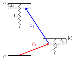
Figure 1: Three level excitation scheme. A red laser (red) excites from the ground state $|g\rangle$ to an intermediate state $|e\rangle$ and is detuned by $\Delta_{1}$. Another laser will excite from this intermediate level to the Rydberg level $|r\rangle$ and is detuned by $\Delta_{2}$.

This paper is structured into seven sections. In section II we will derive the (de-) excitation rates for a single atom influenced by lasers as indicated Figure 1, and in section III we investigate the limits to the rate equation model (RE) in depth. In section IV we investigate the differences in a Monte Carlo simulation, stemming from the three sets of rates. In section VI we draw conclusions on this work.

II Rate equations

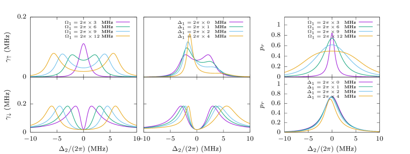
Figure 2: Excitation rates (top) and deexcitation rates (bottom) vs blue detuning $\Delta_{2}$, for different sets of laser parameters. Left column: Varying red Rabi frequency $\Omega_{1}$, with constant blue Rabi frequency $\Omega_{2}=2\pi\times 0.4$ MHz and red detuning $\Delta_{1}=2\pi\times 0$ MHz. Middle column: Varying red detuning $\Delta_{1}$, with constant blue Rabi frequency $\Omega_{2}=2\pi\times 0.4$ MHz and red Rabi frequency $\Omega_{1}=2\pi\times 6$ MHz. Right column: Steady state Rydberg populations, while varying red Rabi frequency (top) or red detuning (bottom). Other parameters are as in the corresponding (de-)excitation column.

We base our approach on $N$ three level atoms with the Hamiltonian of the $i^{\text{th}}$ atom in the interaction picture given by

$$H^{i}= \frac{\hbar}{2}\bigg{(}-\Delta_{1}|e_{i}\rangle\langle e_{i}|-\Delta_{2}|r_{i}\rangle\langle r_{i}|$$

$$+\Omega_{1}|g_{i}\rangle\langle e_{i}|+\Omega_{2}|e_{i}\rangle\langle r_{i}|+\text{H.C.}\bigg{)}$$ (1)

with $|e_{i}\rangle$ ($|r_{i}\rangle$) the $i^{\text{th}}$ atom being in the intermediate (Rydberg) state. Other authors have used similar rate equation models for two-level Lesanovsky and Garrahan (2014); Gärttner et al. (2014) or three-level Ates et al. (2007b, a); Heeg et al. (2012); Ates et al. (2011) atoms. In Refs. Ates et al. (2007b, a); Heeg et al. (2012) an effective two-level system is achieved by fixing the intermediate level detuning at zero. Our three-level atom rate equation model allows for both the Rydberg and intermediate level detunings to be freely chosen input parameters, as well as both Rabi frequencies and the spontaneous decay rates. Further, we treat in some detail the limits of this free choice in the next section.

In the following sections, the parameters of the three-level atom model will be loosely based on the parameters of our ⁸⁵Rb experiment. Then in Section V we will discuss the validity of this model in the context of a particular experimental realisation. The intermediate state is given by $5P_{3/2}$, and for now the Rydberg state is specified as $100S_{1/2}$. These states have spontaneous decay rates $\Gamma_{e}=2\pi\times 6.07$ MHz for the intermediate state and $\Gamma_{r}=2\pi\times 0.003$ MHz for the Rydberg state. We call the laser associated with subscript 1 the probe laser and the one associated with subscript 2 the coupling laser. The interactions between atoms are given by

$$H^{i}_{\text{int}} =\frac{1}{2}\sum_{\begin{subarray}{c}j\neq i\end{subarray}}^{N}\frac{C_{6}}{r_{ij}^{6}}|r_{j}\rangle|r_{i}\rangle\langle r_{i}|\langle r_{j}|,$$ (2)

where $r_{ij}$ is the distance between atoms $i$ and $j$, and $C_{6}$ is the van der Waals coefficient scaling as the principal quantum number of the Rydberg state $|r\rangle$ to the power of $11$. Since this work is done with a specific ultra cold gas experiment in mind, we apply the frozen gas approximation and assume the $r_{ij}$s to stay constant and the terms of $H_{\text{int}}^{i}$ can be evaluated only once. The state of the system determines what terms to be included at any given time. We will assume that each atom can be modeled independently, with only an effective shift in local coupling detuning due to the interactions between Rydberg atoms. The entire effect of $H_{\text{int}}^{i}$ is then captured by modifying the coupling detuning since we consider istropic interactions only:

$$\Delta_{2}\rightarrow\Delta_{2}+\frac{1}{\hbar}\langle\bm{s}|H_{\text{int}}^{i}|\bm{s}\rangle=\Delta^{i}_{\text{eff}}(\bm{s}),$$ (3)

where $|\bm{s}\rangle$ is the state of the full $N$ atom system, if atom $i$ is excited.

Using these we find the master equation (ME) of atom $i$ in Lindblad form

$$\frac{d}{dt}\rho= -\frac{i}{\hbar}[H^{i}(\bm{s}),\rho]+\mathcal{L}(\rho),$$ (4)

where $H^{i}(\bm{s})$ given by eq. (1) with the replacement eq. (3) and Liouvillian

$$\mathcal{L}(\rho)= \Gamma_{e}|e_{i}\rangle\langle g_{i}|\rho|g_{i}\rangle\langle e_{i}|-\frac{\Gamma_{e}}{2}\{\rho,|e_{i}\rangle\langle e_{i}|\}$$

$$+ \Gamma_{r}|r_{i}\rangle\langle e_{i}|\rho|e_{i}\rangle\langle r_{i}|-\frac{\Gamma_{r}}{2}\{\rho,|r_{i}\rangle\langle r_{i}|\},$$ (5)

and $H^{i}(\bm{s})$ being the Hamiltonian in eq. (1) with $\Delta_{2}$ replaced by the state dependent effective detuning eq. (3).

Rewriting the density matrix of a single atom in vector form, the effective time evolution operator is

$$\dot{\bm{\rho}}=\mathcal{R}\bm{\rho}=\begin{pmatrix}\mathcal{R}_{p}&L\\ L^{T}&\mathcal{R}_{c}\end{pmatrix}\bm{\rho},$$ (6)

with $\bm{\rho}^{T}=(\rho_{gg},\rho_{ee},\rho_{rr},\rho_{ge},\rho_{er},\rho_{gr},\rho_{eg},\rho_{re},\rho_{rg})$, $\mathcal{R}_{p}$ is a $3\times 3$ matrix taking population to populations, $\mathcal{R}_{c}$ is a $6\times 6$ matrix taking coherences to coherences and $L$ is a $3\times 6$ matrix taking coherences to populations. Adiabatically removing the coherences, which is permitted when the time scale of the dynamics in the coherences is much smaller than the time scale of the population dynamics, we can write the optical Bloch equations

$$\dot{\bm{p}}=\left(\mathcal{R}_{p}-L\mathcal{R}_{c}^{-1}L^{T}\right)\bm{p}=Q\,\bm{p},$$ (7)

where $\bm{p}=(p_{g},p_{e},p_{r})^{T}$ are the populations ($\rho_{gg}$, $\rho_{ee}$ and $\rho_{rr}$) of the $i^{\text{th}}$ atom. Our analysis has shown that, for laser parameters where adiabatic elimination of the coherences is valid, the elements of $Q$ solely associated with the dynamics between $p_{g}$ and $p_{e}$ are larger than those associated with dynamics of $p_{r}$ by two or three orders of magnitude. We will call the terms associated with the dynamics of $p_{r}$ the ’small’ terms of $Q$.

The general solution to such a homogeneous system of coupled differential equations is known

$$\bm{p}=\sum_{k}\bm{v}_{k}\exp\left(-\lambda_{k}t\right),$$ (8)

with $\lambda_{k}$ ($\bm{v}_{k}$) the eigenvalues (-vectors) of $Q$, and the sum running over all eigenvalues. At sufficiently long time, all but one (non-zero) eigenvalues have dampened out, and we know that $\dot{p}_{r}=\alpha\dot{p}_{e}$, where $|\alpha|\gtrsim 1$, since only one eigenvector contributes to the derivative. From this we can express $p_{e}$ in terms of $p_{r}$ and $Q$

$$p_{e}= \frac{(0,1,0)\,Q\,(1,0,0)^{T}}{(0,1,0)\,Q\,(-1,1,0)^{T}}\,(1-p_{r}),$$ (9)

by neglecting the small entries in the matrix $Q$.

We define excitation rate $\gamma_{\uparrow}$ and deexcitation rate $\gamma_{\downarrow}$, such that

$$\dot{p}_{r}=\gamma_{\uparrow}(p_{g}+p_{e})-\gamma_{\downarrow}p_{r}=\gamma_{\uparrow}(1-p_{r})-\gamma_{\downarrow}p_{r},$$ (10)

which can be found by substituting eq. (9) into eq. (7) to get

$$\gamma_{\uparrow}= (0,-\xi,1)\,Q\,(1,0,0)^{T}$$ (11)

$$\gamma_{\downarrow}= (0,0,1)\,Q\,(\xi-1,-\xi,1)^{T}.$$ (12)

with

$$\xi= \frac{(0,1,0)\,Q\,(-1,0,1)^{T}}{(0,1,0)\,Q\,(-1,1,0)^{T}}.$$ (13)

For the steady state solution the time derivative is the null-vector, and we get

$$p_{r}^{\infty}=\frac{\gamma_{\uparrow}}{\gamma_{\uparrow}+\gamma_{\downarrow}}.$$ (14)

In Fig. 2 we show the derived (de-) excitation rates versus the blue laser detuning $\Delta_{2}$ for a variety of laser parameters. In the left and middle column only a single of the three remaining controllable parameters is varied and the others are kept constant at $\Omega_{1}=2\pi\times 6$ MHz, $\Delta_{1}=0$ MHz and $\Omega_{2}=2\pi\times 0.4$ MHz. In the right most column the corresponding steady state populations are shown. We observe that the excitation rates show the general features we expect, like Autler-Townes splitting into two Lorentzian peaks for $\Omega_{1}>\Gamma_{e}$ and tend to 0 for large Rydberg detuning $\Delta_{2}$. For small $\Omega_{1}$, the two Lorentzian peaks merge, as expected. For large intermediate state detuning $\Delta_{1}$, the center of the largest peak shifts towards larger Rydberg detuning by a value of $\Delta_{1}/2$ and the peak to peak distance is $\sqrt{\Omega_{1}^{2}+\Omega_{2}^{2}+\Delta_{1}^{2}}$. Further, the ratio between the maximal height of the two peaks tends to zero. These features are easily explained from the eigenvalues and -states of the Hamiltonian (1). For the de-excitation rates we generally observe the same with two important addenda. First, for large Rydberg detuning $\Delta_{2}$, the de-excitation rate does not go to zero, but rather $\Gamma_{r}$, as expected. Secondly, for small Rydberg detuning, the de-exitation also approaches the spontaneous decay rate $\Gamma_{r}$. This happens as the de-excitation rate only has an effect on the Rydberg state, which for zero detuning has an overlap with a dark state of the Hamiltonian (1) larger than $0.99$, meaning that the lasers have no influence on the de-excitation rate in this case, reducing the de-excitation rate to the spontaneous decay rate.

The Rydberg populations, as shown in the rightmost column of Fig. 2, are found using Eq. (14). Increasing the red Rabi frequency $\Omega_{1}$ beyond the intermediate state spontaneous decay rate $\Gamma_{e}$ broadens and lowers the Rydberg transition resonance, as Autler-Townes splitting affect the excitation rate. Increasing the intermediate state detuning, lowers and narrows the Rydberg transition resonance, but only slightly, as well as giving a slight shift to the resonance.

III Rate equation validity

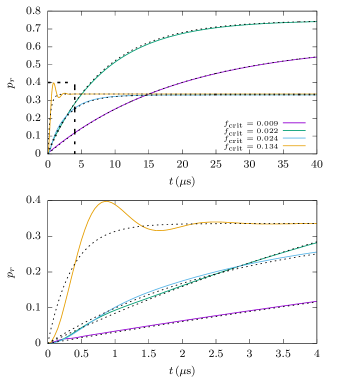
Figure 3: Numerical solutions to the optical Bloch equation (solid) and rate equation approximations (dotted) versus time for different critical fractions $f_{\text{rm}}$. Bottom plot shows a magnification indicated by dashed square. Lines with small critical fraction show good agreement between rate equations and optical Bloch equations, whereas the large critical fraction line only shows good agreement with final population value.

Going back to eq. (6) and considering the adiabatic elimination of the coherences, we know that $\mathcal{R}$, has nine complex eigenvalues $v_{1},\dots,v_{9}$ and the coherence only part $\mathcal{R}_{c}$ six complex eigenvalues $k_{1},\dots,k_{6}$, which determine the time scale of the dampening of the coherences. This time scale has to be short, in order to support adiabatic elimination of the coherences. Of the eigenvalues $v_{1},\dots,v_{9}$, only three have eigenvectors with non-zero populations of the intermediate state, and of these only one is always real valued, we call this $v_{1}$. In addition one eigenvalue, which we call $v_{9}$, is always zero.

We define the dampening time scales for eigenvalue $v$ as $\tau_{v}=\frac{-1}{\Re(v)}$, and make shorthands for the three most important

$$\tau_{0}= \tau_{v_{1}}$$ (15)

$$\tau_{1}= \max(\tau_{v_{2}},\dots,\tau_{v_{8}})$$ (16)

$$\tau_{2}= \max(\tau_{k_{1}},\dots,\tau_{k_{6}}).$$ (17)

Since $\tau_{0}$ is, in general, larger than $\tau_{1}$, it is the time scale on which higher order dynamics of the system dampens out and only the steady state solution remains. On top of this the coherences dampen out on the time scale $\tau_{2}$.

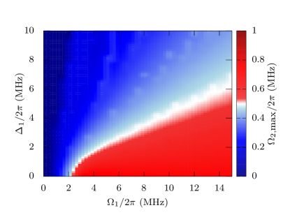
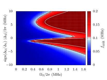
Figure 4: Top: Maximal allowed blue Rabi frequency $\Omega_{2}$ versus red Rabi frequency $\Omega_{1}$ and red detuning $\Delta_{1}$. This value is found as the largest blue Rabi frequency for which the critical fraction is smaller than $0.1$ for all (positive) blue detunings $\Delta_{2}$. Bottom: Critical fraction $f_{\textrm{crit}}$ in the $\Omega_{2}$-$\Delta_{2}$ plane for $\Omega_{1}=2\pi\times 5$ MHz and $\Delta_{1}=2\pi\times 5$ MHz. Black contour line is at $f_{\textrm{crit}}=0.1$ and white at $f_{\textrm{crit}}=0.2$.We generally require that $f_{\textrm{crit}}<0.1$. Note that the positive detunings allow for larger $\Omega_{2}$, but since the sign is dependent on the ratio between the detunings, we can always choose positive for a given experiment.

The rate equation model is dependent on there being a clear distinction between the dynamics on the long time scale $\tau_{0}$ and the shorter time scales $\tau_{1}$ and $\tau_{2}$, and this means that we now have conditions for the validity of the rate equation model

$$\tau_{0}>> \max(\tau_{1},\tau_{2})$$ (18)

$$t>> \tau_{1},$$ (19)

where $t$ is the simulation run time. For practical purposes, we will assume this to be satisfied if

$$f_{\textrm{crit}}=\frac{\max(\tau_{1},\tau_{2})}{\tau_{0}}<0.1,$$ (20)

which we call the critical fraction. Fig. 3 shows a comparison between our rate equation model (dotted) and the optical Bloch equations (solid) for different critical fraction values. The agreement between solid and dotted lines is clearly dependent on the critical fraction. Of special note is the rather bad agreement between the solid and dotted lines for critical fraction larger than $0.1$, which we choose as the practical limit.

We have searched the parameter space to satisfy these conditions, and the requirements are in general quite lax for reasonable red laser parameters, see Fig. 4. For any given combination of red Rabi frequency and detuning, we find the critical fraction in the $\Omega_{2}$-$\Delta_{2}$ plane, and determine the maximal allowed blue Rabi frequency $\Omega_{2,\textrm{max}}$ as the largest value of $\Omega_{2}$ for which the critical fraction is smaller than $0.1$ for all (positive) blue detunings $\Delta_{2}$.

The maximal blue Rabi frequency is dependent on the relative sign of blue detuning to red detuning, and we can find blue Rabi frequency limits $\Omega_{b}^{+}$ and $\Omega_{b}^{-}$, dependent on that sign, below which the rate equations always hold. This asymmetry is resulting from the asymmetry in the excitation due to the red laser. Since $\Omega_{b}^{+}\geq\Omega_{b}^{-}$ is always the case, we can choose the sign of the red detuning such that we have the largest allowed range for $\Omega_{b}$. However, if scanning the blue detuning across the resonance, the blue Rabi frequency has to be below $\Omega_{b}^{-}$, as the limiting point is right below zero. Note that for most detunings, the maximal blue Rabi frequency can be much larger than this limiting value, and it would be prudent for any experiment to determine the limiting values appropriate for the specific experiment.

IV Monte Carlo simulation

We have implemented our (de-)excitation rates in a kinetic Monte Carlo simulation, where we extract the values of interest as the average over many realizations. We will explore three different settings, first we consider a 1D regular lattice, secondly a random gas with a square quasi 2D excitation volume and finally we will compare to experimental measurements. The calculations are based on a long-range van der Waals interaction for two ⁸⁵Rb atoms in the n=100$S_{1/2}$ state, with a van der Waals coefficient $C_{6}=56$ THz $\mu$m⁶ Šibalić et al. (2017).

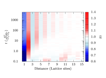
Figure 5: Time dependence of excitation probability in the 1D lattice with 30 lattice sites. Labels denote lattice site. Probability is calculated as the number of Monte Carlo realizations with a Rydberg excitation at a site divided by the total number of realizations for every time step.

Figure 6: Time dependence of the $g_{2}$ function for a 1D lattice with 30 lattice sites. Nearest neighbors are never Rydberg pairs, but for times larger the equilibration time $T=4\Gamma_{e}/\Omega_{1}\Omega_{2}$ Rydberg excitations start to come in pairs separated by one atom and at $10T$ the crystal consists of 3 excitations. The correlation length scales as $t^{1/3}$, but saturates at $t\sim 100T$.

Each Monte Carlo realization is performed by, at time $t_{0}=0$, calculating (de-)excitation rates for all atoms and an exponentially distributed random time step $dt$, with mean value $1/\sum_{i}\gamma^{i}_{\updownarrow}$, with $\gamma^{i}_{\updownarrow}$ the excitation rate for atom $i$ (deexcitation rate if atom $i$ is already excited). We then randomly pick an atom with probability proportional to the $\gamma^{i}_{\updownarrow}$. This atom is then (de-)excited and the time is set to $t_{1}=t_{0}+dt$. This procedure is then repeated until the time exceeds the simulation time $t_{\textrm{end}}<t_{\textrm{end}-1}+dt$. At prespecified times, we save the state of the system for our analysis. The output of the Monte Carlo simulation is the average over all realizations.

For our 1D lattice simulation, the individual lattice sites are identifiable and we therefore explore the time evolution of the excitation probability of the individual sites. This requires many realizations to converge and we therefore perform 6000 realizations for the simulation. For a realised population of 0.5, the statistical error bar for this number of realisations is about $2\%$.

We consider a string of 30 atoms placed at regular distance $l=16.3\,\mu\textrm{m}$ with laser parameters $\Omega_{1}=\Gamma_{e}/2$, $\Omega_{2}=\Gamma_{e}/10$, $\Delta_{1}=\Delta_{2}=0$. This results in a nearest neighbor interaction strength $V_{nn}=2\Omega_{1}$ for the $100S$ state and corresponds to the work done in Höning et al. (2013). Our work is consistent with their result, but for a slightly larger correlation length due to the fully interacting system.

On time scales on the order of the steady-state equilibration time for a single atom $T=4\Gamma_{e}/\Omega_{1}\Omega_{2}$, the system reaches a $1-e^{-1}$ fraction of its final Rydberg population, but this is distributed over many single atom excitations. At such small time scales, only the edge atoms have a larger than average Rydberg probability, as they only have neighbors on one side, see Fig. 6. On time scales of $3T$, we observe the first formation of small local crystalline structures with correlation lengths larger than 1 lattice constant and growing as $t^{1/3}$, see Fig. 6, consisting of two Rydberg excitations separated by a single unexcited lattice site. The second-order spatial correlation function $g_{2}$ shown in this figure, and also later in Fig. 7, is a measure for the correlations in the distances between two Rydberg atoms. It can be found by binning the relative distances of Rydberg pairs, and counting the number of these pairs for these binned distances. This distribution is then normalized with respect to the distribution of Rydberg pairs between uncorrelated simulations. For the 1D lattice, these bins are naturally provided by the discrete separation distance measured in lattice sites. These structures are not all consistent with a global crystal, as they have formed at random positions in the lattice and could lead to domains in the final state. At this time, the enhanced Rydberg probability of the edge sites leads to suppression of the Rydberg probability of their neighbors. This effect is the beginning of the global crystal structure.

These small crystals will continuously form and melt in the lattice at random positions, but as time passes, fewer and fewer sites not consistent with a larger crystal will be available, and at time scales of $10T$ the average crystal formation will contain three Rydberg atoms. As the process continues, the crystal forming on the edge grows, as there is no room for excitation hopping, and the average crystal size increases. At large time scales ($\sim 100T$), a global crystal has formed by spanning the entire lattice, and the correlation length does not increase further.

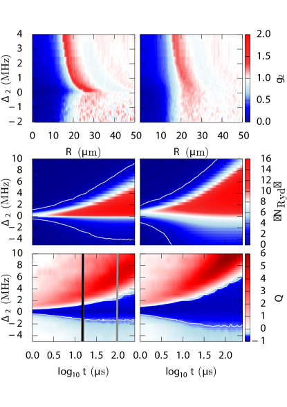
Figure 7: Statistical measures of Rydberg excitation for a Gaussian profile red laser beam (left) and a uniform square laser beam (right). Top row: $g_{2}$ map as function of detuning $\Delta_{2}$ and relative position $R$. In both cases we observe clear blockade for small distances $R$ followed by a uniform distribution for negative blue detuning ($\Delta_{2}<0$) and strong facilitation for positive blue detuning. Middle row: Average Rydberg count across all realizations as function of detuning $\Delta_{2}$ and time $t$. White contours mark $\langle N_{\textrm{Ryd}}\rangle=1$. Large Rydberg populations do not appear for large negative detuning and appear explosively but delayed for positive detunings. Note that the square geometry has about half the number of atoms in the excitation volume and hence twice the Rydberg fraction. Bottom row: Mandel $Q$-parameter as function of detuning $\Delta_{2}$ and time $t$. Dark blue is $Q<-1/2$, the deeply subpoissonian regime. For positive detuning $Q>0$, we are in the superpoissonian regime (red). Two different times are indicated by vertical lines, 15$\mu$s (black) and 106$\mu$s (gray), for a direct comparison to the same times in Fig. 8.

We move on to our quasi 2D random gas, which we will use to model the conditions in a magneto optical trap (MOT), and consider three statistical properties: Average Rydberg count $\langle N_{\textrm{Ryd}}\rangle$, Mandel $Q$-parameter and second-order spatial correlation function $g_{2}$.

We perform each Monte Carlo realization with a total simulation time $t_{\textrm{end}}=250\,\mu$s, a total number of atoms $N_{\text{tot}}$ equal to the integral of the atomic density in the laser volume. The total number of realizations is 2500 for every set of parameters. Additionally, we assume the gas to be cold enough that we can ignore all atomic motion.

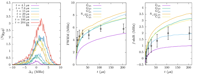
Figure 8: Left: Rydberg spectra in experiment (solid) with laser parameters $\Omega_{1}=2\pi\times 4$ MHz, $\Omega_{2}=2\pi\times 0.5$ MHz and $\Delta_{1}=-2\pi\times 9$ MHz and the red Gaussian profiled laser, with waist $\sigma_{\textrm{red}}=25\,\mu$m, intersects a Gaussian profile blue sheet with waist $\sigma_{\textrm{blue}}=7\,\mu$m, corresponding to the simulations in Fig. 7. Dashed curves are skew-Gaussian fits. Middle: Full width half max of the experimental spectrum (circles), errorbars determined from fit, and simulation (solid) of Gaussian (G), square (S) or circular (C) laser beam profiles with the characteristic length scale (std for Gaussian, side length for square and radius for circular) denoted by subscript. The star ($*$) denotes simulation with twice the red laser intensity ($\Omega_{1}\rightarrow\sqrt{2}\Omega_{1}$). Right: Frequency shift of the experimental spectrum (circles), errorbars determined from fit and frequency drift of the blue laser. Solid curves represent the same simulations as in middle plot. The overall comparison between experiment and simulation show general agreement for both FWHM and frequency shift.

We excite to the $99S$ state and use laser parameters according to our experimental setup: $\Omega_{1}=2\pi\times 4$ MHz, $\Omega_{2}=2\pi\times 0.5$ MHz, $\Delta_{1}=-2\pi\times 9$ MHz and the blue laser detuning $\Delta_{2}$ is variable. The red laser intersects a Gaussian blue sheet with waist $\sigma_{\textrm{blue}}=7\,\mu$m. Due to the thickness of the blue sheet, we do not expect the second order correlation function $g_{2}$ to be zero inside the blockade radius, but strongly suppressed, since we only explore the correlations in the projection on the blue laser plane. In Fig. 7, we show results from two different red laser geometries, realizable in our experiment by means of a spatial light modulator, a Gaussian beam profile with waist $\sigma_{\textrm{red}}=25\,\mu$m (left in Fig. 7) and a square beam profile of uniform intensity with side length $l=\sqrt{2\pi}\,25\,\mu$m (right in Fig. 7). These shapes ensure the two lasers output the same power, but the Gaussian excitation volume has about twice the number of atoms compared to the square geometry. Our model is not limited to these laser shapes and parameters, but they show the essential features. Since the blockade radius $R_{\textrm{block}}$, for the given parameter and $\Delta_{2}=0$, is $20.9\,\mu$m, we expect the system to be completely filled at $N_{\textrm{Ryd}}=(l/R_{\textrm{block}})^{2}\approx 9$ for the square beam profile and slightly before that for the Gaussian beam profile, we call this number the jamming count $N_{\textrm{Jam}}$.

We start by generating $N_{\text{tot}}$ random 3D coordinates in the laser volume, and we calculate the laser parameters at each coordinate as well as the distances between all pairs of atoms. With these parameters in place at the beginning of each realization it is easy to evaluate the (de-)excitation rates at each atom on the fly.

For any specific realization we are only interested in the Rydberg count and distribution at a number of prespecified time steps, therefore we only carry the binary information of Rydberg state or ground state for each atom, as well as the atom positions. This will let us determine both the Rydberg-Rydberg interaction strength at each coordinate from the predetermined atomic distances, for use in determining the rates, and is sufficient to calculate the aforementioned statistical measures we are interested in for the total ensemble of realizations, see Fig. 7.

Analyses of the Monte Carlo simulations show features usually associated with the Rydberg-Rydberg interaction, but also illustrates a clear dependence on excitation geometry. The location of the first excitation is much more likely to occur near the center of the excitation volume for the Gaussian profile beam. For negative detunings this leads to even stronger blockade as not only is the effective detuning larger, but the Rabi frequency is also lower. For positive detunings, however, the facilitation rings become narrower. The gradient of the laser intensity also leads to a tighter distribution of excitations, as excitation too far from the center is unlikely, limiting the number of excitations in the volume.

From the Mandel $Q$-parameter, see Fig. 7 (bottom), we can identify three regimes of interest: Firstly, the (weakly sub)poissonian (light blue) regime where $-1/2<Q<0$, found for very low blue laser detunings $\Delta_{2}$. Secondly, the deeply subpoissonian (dark blue) regime where $Q<-1/2$, found for small absolute values of $\Delta_{2}$. And thirdly, the superpoissonian (red) regime where $Q>0$, found for large positive $\Delta_{2}$.

For negative blue laser detunings, the Mandel $Q$-parameter gradually decreases over time from 0 to its final value. This happens as atoms are excited to the Rydberg state and exclude parts of the volume. For very negative detunings, only a few Rydberg excitations exist at any given time and the $Q$-parameter stays relatively high, since the jamming limit is never reached. This is again reflected in the average Rydberg count, which is very low compared to the jamming count $N_{\textrm{Jam}}$.

For detunings closer to zero, the number of Rydberg excitations increases over time and the jamming limit is reached, resulting in deeply subpoissonian counting statistics. The subpoissonian regime is reached somewhat before the jamming count, since the reduction in the excitation volume is significant when $N_{\textrm{Ryd}}\geq\sqrt{N_{\textrm{Jam}}}$.

For positive blue laser detunings, an initial Rydberg excitation, called the seeding excitation, results in a ring of resonant excitation around the seed at the distance $R=(C_{6}/\Delta_{2})^{1/6}$, called the facilitation distance $R_{\textrm{fac}}$. The seeding excitation occurs with low probability for large detunings, but after seeding more Rydberg atoms are quickly excited on resonance. This results in superpoissonian counting statistics, as a cascade of Rydberg excitations spreads from the seed. We can observe this in the steep slope of the average Rydberg count for positive detuning coinciding with very large Mandel $Q$-parameter. However, the system quickly fills up, reaching the jamming limit resulting in a drop to negative $Q$ and the strongly subpoissonian regime.

The second order correlation functions $g_{2}$ at time $t=250\,\mu$s for the Gaussian (left) and square (right) beam profiles are seen in Fig. 7 (top). For negative blue laser detuning, the region in the immediate vicinity of a Rydberg excitation ($R\lesssim R_{\textrm{block}}=21\,\mu$m) shows very reduced values of $g_{2}$. Around $R_{\textrm{block}}$, the $g_{2}$ gradually climbs to 1, with only a slight overshoot. This behavior is the same for both geometries and consistent with the blockade effect. The nonzero value for short distances is due to the thickness of the excitation volume, as we only consider the correlations in the plane parallel to the blue laser sheet.

For positive blue laser detuning the blockade effect is still clearly visible for small distances, but at the facilitation distance $R_{\textrm{fac}}\approx(C_{6}/\hbar\Delta_{2})^{1/6}$ there is a strong signal from the facilitation region followed by a dip from the blockade effect of the facilitated excitations. This feature is significantly sharper for the Gaussian geometry consistent with a narrower facilitation region due to the drop off in laser intensity. At about $2R_{\textrm{fac}}$, a faint signal from the secondary facilitation peak is visible for both the Gaussian and the square beam profiles.

At very limited blue laser detunings ($|\Delta_{2}|\lesssim 0.5$ MHz) the $g_{2}$-function resulting from the Gaussian beam profile shows a cusp that is not present in case of a square beam profile. This cusp is in part due to the sharpening of the facilitation peak in the Gaussian profile case and in part due to the tighter packing of Rydberg excitations for the Gaussian beam profile. This leads to a crystalline locking of the Rydberg excitations in the relatively small volume of peak laser intensity.

V Experimental comparison

Rydberg excitation was studied experimentally using a setup described previously Engelen et al. (2014); M. W. van Bijnen et al. (2014). In short, ⁸⁵Rb atoms are trapped and cooled in a standard magneto-optical trap, resulting in typical atomic densities of $10^{16}/$m³ and temperatures of $0.2$ mK. To create Rydberg atoms from the cooled sample, the 780nm trapping laser beams are suddenly switched off, after which a separate 780 nm and a 479 nm laser beam are flashed on for a variable amount of time, which drive the $5S,F=2\rightarrow 5P_{3/2},F=3$ and $5P_{3/2},F=3\rightarrow 99S$ transitions in ⁸⁵Rb. The red laser beam is referenced to the atomic transition frequency by a saturated absorption scheme, and detuned approximately 9 MHz below resonance. The frequency of the blue laser can be scanned in a range of tens of MHz centered on the two-photon resonance condition and is referenced to a commercial ultrastable cavity (Stable Laser Systems). The linewidths of the two laser beams are below 1 MHz but otherwise not accurately known.

The red laser beam can be spatially shaped using a spatial light modulator M. W. van Bijnen et al. (2014) in various ways but in the experiments reported here the spatial shape was a single Gaussian with a rms radius of $25\,\mu$m. This shaped red beam crosses the blue beam at the center of the MOT, where the rms sizes of the blue beam are $7\,\mu$m $\times 1.8$ mm. Typical excitation times are in the $\mu$s range. The powers of the laser beams were adjusted to provide nominal Rabi frequencies of $\Omega_{1}\approx 4$ MHz and $\Omega_{2}\approx 0.5$ MHz.

Rydberg atoms created by this excitation sequence were detected using field ionization. An electric field of several kV/m strength is turned on which ionizes any Rydberg atoms present and pushes the resulting ions towards a dual microchannel-plate detector (GIDS GmbH) Engelen et al. (2014). The current produced by the detector is fed through a transimpedance amplifier and then sampled by a digital oscilloscope (Agilent DSO 054A). The integral of the digitized signal over a period of the experimental cycle is taken as proportional to the number of Rydberg atoms produced.

The experiment does not strickly fullfil all conditions assumed in the model. E.g., in our model we assume the frozen gas limit to hold. The experiment operates at a temperature of $T=0.2$mK, so that atoms travel the average separation in 50$\mu$s. The time scale set by the rates in Fig. 2, however, is only a few microseconds, which then sets the time that an atom spends in a Rydberg excitation. During this time the atoms move over a distance of up to a micrometer, which is much smaller than the mean interparticle separation and justifying the frozen gas limit approximation. Note that the coherence time is even smaller, as can be seen from Fig. 3.

Second, for the total decay rate $\Gamma_{r}$ we took both spontaneous emission and losses from black-body radiation into account. Although this gives rise to a correct lifetime of the Rydberg state, the inclusion of black-body radiation, which dominates the lifetime, is not fully consistent as it does not provide a direct decay to the intermediate state but rather a transition to nearby excited levels. However, these levels will eventually also decay. Also the expression for the van der Waals interaction does not hold up exactly at short distances as other levels are getting nearby. For n=99 the closest pair is 99$P_{3/2}$+98$P_{3/2}$ at an energy of 215 MHz Šibalić et al. (2017), which is equivalent to the van der Waals energy for two n=99 pairs for a spacing at 8 $\mu$m. However, the repulsive character is maintained, and at this distance the particles are already deeply in the blockaded regime.

Experimentally observed spectra are shown in Fig. 8 (left), and fitted with a skew Gaussian. From this fit the derived parameters of full width half max (FWHM) (middle) and frequency shift ($f$-shift) (right) are determined and plotted (circles). The errorbars on the FWHM values are determined from the 95% confidence limit of the fitting parameters (fitting error). The $f$-shift errorbars are determined as the root of the sum of the fitting error squared and the measurement error squared. The derived parameters from the experiment are compared to simulation (solid). We show here derived parameters for both the Gaussian and the square laser profile simulations of Fig. 7 as well as those from a simulation with the same Gaussian laser profile, but twice the intensity, ie. $\Omega_{1}\rightarrow\sqrt{2}\Omega_{1}$.

Direct comparison between the experimental (see Fig. 8, left) and simulated (Fig. 7, middle) spectra shows a general agreement. Far from resonance ($|\Delta_{2}|\gtrsim 8$ MHz) the experimental Rydberg count is suppressed at all times. For negative Rydberg detuning ($\Delta_{2}\lesssim-2$ MHz) we see suppression of the increase in Rydberg count over time, consistent with the existing Rydberg atoms in the volume blocking excitation of additional Rydberg atoms. Nearing zero detuning ($|\Delta_{2}|\lesssim 2$ MHz) the Rydberg count grows fast and the peak shifts towards higher detunings with time. This means that, especially at later times, the peak is shifted to large Rydberg detuning ($\Delta_{2}\gtrsim 2$ MHz). At these large detunings, we observe almost no Rydberg atoms at small times, but with increasing time this changes as facilitation shifts the Rydberg levels of unexcitated atoms into resonance. This is all in agreement with the simulation results presented in Fig. 7.

For both experimental data and simulation we observe that both the FWHM and $f$-shift, derived from the spectra in Fig. 8, values rise quickly and then level out after about 50$\,\mu$s. The precise shape of the excitation volume and laser profile have little influence on the behavior of the FWHM value, and we can generally explain experimental observations without knowledge of the exact excitation volume geometry. Similarly, the $f$-shift shows some dependence on the laser profile, but this can be explained from the small dependence of Rydberg count on geometry to influence the $f$-shift.

VI Conclusions

We have derived rate equations for excitations of the Rydberg state in three-level atoms starting from the master equation. Our approach does not assume vanishing populations in the intermediate state and are therefore valid for a wide range of laser parameters, in principle whenever the three-level approximation of the atom is valid.

Our rate equation model agrees with the master equation, provided that only one eigenvalue has not dampened out. We have investigated and described the validity range of our approach, and determined criteria that provide sufficient insight into whether our model is valid or full solution of the master equation is required.

We have made a Monte Carlo implementation of our (de-)excitation rates, and explored different excitation geometries and laser parameters. In this paper we have reported on 1D lattice simulations, with parameters corresponding to previous theoretical work published in Höning et al. (2013), and found our results to be consistent with literature. We explored the dynamics of self assembly of the resulting 1D Rydberg crystal, and the time evolution of the second order correlation function $g_{2}$ and site dependent excitation probability.

We further explored 2D settings, where we considered the effect of the laser beam profile by comparing a Gaussian profile to a square of uniform intensity with sharp edges. We found that the beam profile has significant influence on the resulting excitation pattern and that a Gaussian profile in general will result in sharper features in the $g_{2}$-map, but at the cost of lower excitation counts.

We have compared our model to experimentally observed Rydberg spectra at several time steps and found a general agreement for the spectral shapes and derived parameters FWHM and $f$-shift. We did not see any significant dependence on excitation volume geometry in the time dependence of FWHM, but the geometry dependence of the Rydberg count may result in a slight geometry dependence of the $f$-shift.