Stereotypical Bias Removal for Hate Speech Detection Task using Knowledge-based Generalizations

Abstract.

With the ever-increasing cases of hate spread on social media platforms, it is critical to design abuse detection mechanisms to pro-actively avoid and control such incidents. While there exist methods for hate speech detection, they stereotype words and hence suffer from inherently biased training. Bias removal has been traditionally studied for structured datasets, but we aim at bias mitigation from unstructured text data.

In this paper, we make two important contributions. First, we systematically design methods to quantify the bias for any model and propose algorithms for identifying the set of words which the model stereotypes. Second, we propose novel methods leveraging knowledge-based generalizations for bias-free learning.

Knowledge-based generalization provides an effective way to encode knowledge because the abstraction they provide not only generalizes content but also facilitates retraction of information from the hate speech detection classifier, thereby reducing the imbalance. We experiment with multiple knowledge generalization policies and analyze their effect on general performance and in mitigating bias. Our experiments with two real-world datasets, a Wikipedia Talk Pages dataset (WikiDetox) of size $\sim$96k and a Twitter dataset of size $\sim$24k, show that the use of knowledge-based generalizations results in better performance by forcing the classifier to learn from generalized content. Our methods utilize existing knowledge-bases and can easily be extended to other tasks.

1. Introduction

Examples	Predicted Hate Label (Score)	True Label
those guys are nerds	Hateful (0.83)	Neutral
can you throw that garbage please	Hateful (0.74)
People will die if they kill Obamacare	Hateful (0.78)
oh shit, i did that mistake again	Hateful (0.91)
that arab killed the plants	Hateful (0.87)
I support gay marriage. I believe they have a right to be as miserable as the rest of us.	Hateful (0.77)

Table 1. Examples of Incorrect Predictions from the Perspective API

With the massive increase in user-generated content online, there has also been an increase in automated systems for a large variety of prediction tasks. While such systems report high accuracy on collected data used for testing them, many times such data suffers from multiple types of unintended biases. A popular unintended bias, stereotypical bias (SB), can be based on typical perspectives like skin tone, gender, race, demography, disability, Arab-Muslim background, etc. or can be complicated combinations of these as well as other confounding factors. Not being able to build unbiased prediction systems can lead to low-quality unfair results for victim communities. Since many of such prediction systems are critical in real-life decision making, this unfairness can propagate into government/organizational policy making and general societal perceptions about members of the victim communities (Hovy and Spruit, 2016).

In this paper, we focus on the problem of detecting and removing such bias for the hate speech detection task. With the massive increase in social interactions online, there has also been an increase in hateful activities. Hateful content refers to “posts” that contain abusive speech targeting individuals (cyber-bullying, a politician, a celebrity, a product) or particular groups (a country, LGBT, a religion, gender, an organization, etc.). Detecting such hateful speech is important for discouraging such wrongful activities. While there have been systems for hate speech detection (Badjatiya et al., 2017; Waseem and Hovy, 2016; Djuric et al., 2015; Kwok and Wang, 2013), they do not explicitly handle unintended bias.

We address a very practical issue in short text classification: that the mere presence of a word may (sometimes incorrectly) determine the predicted label. We thus propose methods to identify if the model suffers from such an issue and thus provide techniques to reduce the undue influence of certain keywords.

Acknowledging the importance of hate speech detection, Google launched Perspective API  in 2017. Table 1 shows examples of sentences that get incorrectly labeled by the API (as on $15^{th}$ Aug 2018). We believe that for many of these examples, a significant reason for the errors is bias in training data. Besides this API, we show examples of stereotypical bias from our datasets in Table 2.

Sample	Classification prob. (Prediction)	Inference
kat is a woman	0.63 (Hateful)	Replacing the name from Kat to Alice should not have resulted in such a difference in prediction probability.
alice is a woman	0.23 (Neutral)
that’s just fucking great, man.	0.80 (Hateful)	Use of the word “fucking” somehow makes the sentence hateful. Similarly, use of the word “shit” abruptly increases the hate probability.
that’s just sad man.	0.24 (Neutral)
shit, that’s just sad man.	0.85 (Hateful)
rt @ABC: @DEF @GHI @JKL i don’t want to fit anything into their little boxes …	0.80 (Hateful)	In the training dataset, the word “@ABC” is mentioned in 17 tweets of which 13 (76%) are “Hateful”. Hence, the classifier associates @ABC with “Hateful”
my house is dirty	0.86 (Hateful)	The words “dirty” and “gotta” are present heavily in instances labeled as hateful in the training dataset. This resulted in the classifier learning to wrongfully infer the sentence as being hateful.
i gotta go	0.71 (Hateful)
damn, my house is dirty. i gotta go and clean it	0.99 (Hateful)

Table 2. Examples of Incorrect Predictions from our Datasets described in Section 5.1

Traditionally bias in datasets has been studied from a perspective of detecting and handling imbalance, selection bias, capture bias, and negative set bias (Khosla et al., 2012). In this paper, we discuss the removal of stereotypical bias. While there have been efforts on identifying a broad range of unintended biases in the research and practices around social data (Olteanu et al., 2018), there is hardly any rigorous work on principled detection and removal of such bias. One widely used technique for bias removal is sampling, but it is challenging to obtain instances with desired labels, especially positive labels, that help in bias removal. These techniques are also prone to sneak in further bias due to sample addition. To address such drawbacks, we design automated techniques for bias detection, and knowledge-based generalization techniques for bias removal with a focus on hate speech detection.

Enormous amounts of user-generated content is a boon for learning robust prediction models. However, since stereotypical bias is highly prevalent in user-generated data, prediction models implicitly suffer from such bias (Caliskan et al., 2017). To de-bias the training data, we propose a two-stage method: Detection and Replacement. In the first stage (Detection), we propose skewed prediction probability and class distribution imbalance based novel heuristics for bias sensitive word (BSW) detection. Further, in the second stage (Replacement), we present novel bias removal strategies leveraging knowledge-based generalizations. These include replacing BSWs with generalizations like their Part-of-Speech (POS) tags, Named Entity tags, WordNet (Miller, 1995) based linguistic equivalents, and word embedding based generalizations.

We experiment with two real-world datasets – WikiDetox and Twitter of sizes $\sim$96K and $\sim$24K respectively. The goal of the experiments is to explore the trade-off between hate speech detection accuracy and stereotypical bias mitigation for various combinations of detection and replacement strategies. Since the task is hardly studied, we evaluate using an existing metric Pinned AUC, and also propose a novel metric called PB (Pinned Bias). Our experiments show that the proposed methods result into proportional reduction in bias with an increase in the degree of generalization, without any significant loss in hate speech detection task performance.

In this paper, we make the following important contributions.

• We design a principled two-stage framework for stereotypical bias mitigation for hate speech detection task.

• We propose novel bias sensitive word (BSW) detection strategies, as well as multiple BSW replacement strategies and show improved performance on existing metrics.

• We propose a novel metric called PB (Pinned Bias) that is easier to compute and is effective.

• We perform experiments on two large real-world datasets to show the efficacy of the proposed framework.

The remainder of the paper is organized as follows. In Section 2, we discuss related work in the area of bias mitigation for both structured and unstructured data. In Section 3, we discuss a few definitions and formalize the problem definition. We present the two-stage framework in Section 4. We present experimental results and analysis in Section 5. Finally, we conclude with a brief summary in Section 6.

2. Related Work

Traditionally bias in datasets has been studied from a perspective of detecting and handling imbalance, selection bias, capture bias, and negative set bias (Khosla et al., 2012). In this paper, we discuss the removal of stereotypical bias.

2.1. Handling Bias for Structured Data

These bias mitigation models require structured data with bias sensitive attributes (“protected attributes”) explicitly known. While there have been efforts on identifying a broad range of unintended biases in the research and practices around social data (Olteanu et al., 2018), only recently some research work has been done about bias detection and mitigation in the fairness, accountability, and transparency in machine learning (FAT-ML) community. While most of the papers in the community relate to establishing the existence of bias (Tatman, 2017; Blodgett and O’Connor, 2017), some of these papers provide bias mitigation strategies by altering training data (Feldman et al., 2015), trained models (Hardt et al., 2016), or embeddings (Beutel et al., 2017). Kleinberg et al. (Kleinberg et al., 2016) and Friedler et al. (Friedler et al., 2016) both compare several different fairness metrics for structured data. Unlike this line of work, our work is focused on unstructured data. In particular, we deal with the bias for the hate speech detection task.

2.2. Handling Bias for Unstructured Data

Little prior work exists on fairness for text classification tasks. Blodgett and O’Connor (Blodgett and O’Connor, 2017), Hovy and Spruit (Hovy and Spruit, 2016) and Tatman (Tatman, 2017) discuss the impact of using unfair natural language processing models for real-world tasks, but do not provide mitigation strategies. Bolukbasi et al. (Bolukbasi et al., 2016) demonstrate gender bias in word embeddings and provide a technique to “de-bias” them, allowing these more fair embeddings to be used for any text-based task. But they tackle only gender-based stereotypes while we perform a very generic handling of various stereotypes.

There is hardly any rigorous work on principled detection and removal of stereotypical bias from text data. Dixon et al.’s work (Dixon et al., 2017) is most closely related to our efforts. They handle stereotypical bias using a dictionary of hand-curated biased words, which is not generalizable and scalable. Also, one popular method for bias correction is data augmentation. But it is challenging to obtain instances which help in bias removal, and which do not sneak in further bias. To address such drawbacks, we design automated techniques for bias detection, and knowledge-based generalization techniques for bias removal with a focus on hate speech detection.

3. Problem Formulation

In this section, we present a few definitions and formulate a formal problem statement.

3.1. Preliminary Definitions

We start by presenting definitions of a few terms relevant to this study in the context of hate speech detection task.

Definition 3.0.

Hate Speech: Hate speech is speech that attacks a person or group on the basis of attributes such as race, religion, ethnic origin, national origin, sex, disability, sexual orientation, or gender identity. Its not the same as using certain profane words in text. A sentence can use profane words and still might not be hate speech. Eg, Oh shit! I forgot to call him

Definition 3.0.

Hate Speech Detection: Hate Speech Detection is a classification task where a classifier is first trained using labeled text data to classify test instances into one of the two classes: Hateful or Neutral.

Definition 3.0.

Stereotypical Bias (SB): In social psychology, a stereotype is an over-generalized belief about a particular category of people. However, in the context of hate speech detection, we define SB as an over-generalized belief about a word being Hateful or Neutral.

For example, as shown in Table 2, “kat” and “@ABC” have a bias of being associated with “Hateful” class. Typical stereotype parameters represented as strings could also pertain to stereotypical bias in the context of hate speech detection, e.g. “girls”, “blacks”, etc.

Definition 3.0.

Feature Units: These are the smallest units of the feature space which are used by different text processing methods.

SB in the context of hate speech detection can be studied in terms of various feature units like character n-grams, word n-grams, phrases, or sentences. In this work, although we focus on words as feature units, the work can be easily generalized to other levels of text.

Definition 3.0.

Bias Sensitive Word (BSW): A word $w$ is defined as a bias sensitive word for a classifier if the classifier is unreasonably biased with respect to $w$ to a very high degree.

For example, if a classifier labels the sentence with just a word “muslims” as “Hateful” with probability 0.81, then we say that the word “muslims” is a BSW for the classifier. Similarly, if a classifier predicts the sentence ‘Is Alex acting weird because she is a woman ?’ with much higher probability than ‘Is Alex acting weird because he is a man ?’ as Hateful, then the words “woman” and “she” are BSWs for that classifier.

3.2. Problem Formulation

Given: A hate speech detection classifier.
Find:

• A list of BSW words from its training data.

• De-biased dataset to mitigate the impact of BSWs.

We propose a two-stage framework to solve the problem. In the first stage (Detection), we propose biased-model prediction based novel heuristics for bias sensitive word (BSW) detection. Further, in the second stage (Replacement), we present novel bias removal strategies leveraging knowledge-based generalizations. Figure 1 shows the basic architecture diagram of the proposed framework.

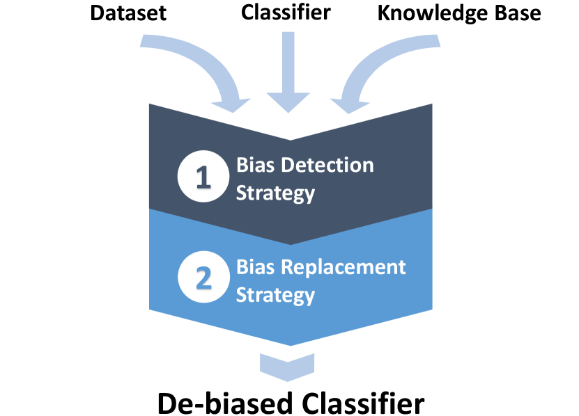
Figure 1. Conceptual Diagram for the proposed 2-Stage De-biasing Framework

4. Two-Stage De-biasing Approach

In this section, we first discuss the first stage of the proposed framework which deals with detection of BSWs. Next, we discuss choices related to bias correction strategies that we could employ. Finally, as part of the second stage, we propose multiple knowledge generalization based BSW replacement strategies.

4.1. Stage 1: Identifying BSWs

Many text-related tasks (e.g., gender profiling based on user-written text, named entity recognition) can extract strong signals from individual word occurrences within the text. However, higher order natural language processing tasks like hate speech detection, sentiment prediction, sarcasm detection cannot depend on strong signals from individual word occurrences; they need to extract signals from a combination of such words. Consider the sentence “Pakistan is a country with beautiful mountains”. Here it is good for a named entity recognition classifier to use its knowledge about the significant association between the word “Pakistan” and a label “location”. But it is not good for a hate speech detection classifier to use its knowledge about associating the word “Pakistan” with label “Hateful” which it might have unintendedly learned from the training data.

Note that although it is important to identify BSWs, it is important to ensure that obvious hateful words should not be removed while doing bias mitigation. Using a standard abusive word dictionary, one can easily ignore such words from being considered a BSW. To identify stereotypical bias and avoid the classifier from propagating the bias from training data to its parameters, we propose the following three strategies for identifying BSWs.

4.1.1. Manual List Creation

Dixon et al. (2017) manually created a set of 50 terms after performing analysis on the term usage across the training dataset. The selected set contains terms of similar nature but with disproportionate usage in hateful comments. Examples: lesbian, gay, bisexual, transgender, trans, queer, lgbt, etc.

4.1.2. Skewed Occurrence Across Classes (SOAC)

If a word is present a significant number of times in a particular class (say Hateful), the classifier is highly likely to learn a high probability of classifying a sentence containing that word into that particular class. Hence, we define the skewed occurrence measure to detect such BSWs.

For the hate speech detection task, consider the two classes: Hateful (+) vs Neutral (-). Let $tf(w)$ be the total term frequency of the word $w$ in the training dataset. Let $df(w)$ be the total document frequency, $df^{+}(w)$ be the document frequency of the word for documents labeled as Hateful, and $df^{-}(w)$ be the document frequency of the word for documents labeled as Neutral. Then, we can use the procedure mentioned in Algorithm 1 to rank the BSWs.

1:  $S$ is a ordered list of words, $tf$ is term-frequency of these words, $df$ is document-frequency values of these words, $\phi$ is the cutoff $tf$ threshold.

2:  $S^{*}\leftarrow\{w|w\in S~{}and~{}tf(w)>\phi~{}and~{}df^{+}(w)>df^{-}(w)\}$

3:  Sort $S^{*}$ in non-ascending order by ($df(w)$, $df^{+}(w)/df(w)$).

Algorithm 1 BSW Detection based on ‘Skewed Occurrence Across Classes’ detection strategy in Training Dataset

Filtering based on just the high frequency would not be enough as that would include stopwords as well, hence we add additional constraints to filter these unnecessary terms.

Essentially, Algorithm 1 ranks a word higher if (1) it occurs with a minimum $\phi$ frequency in the entire dataset (2) it occurs in many training dataset documents (3) it occurs in Hateful documents much more than in Neutral documents. The drawback of this method is that we need to have access to the exact training corpus.

4.1.3. Skewed Predicted Class Probability Distribution (SPCPD)

Let $p(c|w)$ denote the classifier prediction probability of assigning a sentence containing only word $w$ to class $c$. Let $c_{\phi}$ denote a “Neutral” or an “Others” class, or any such “catchall” class. Then, we define the SPCPD score as the maximum probability of $w$ belonging to one of the classes excluding $c_{\phi}$.

(1) $$SPCPD(w)=\max_{\forall c\in C,c\neq c_{\phi}}p(c|w)$$

Note that a high value of $SPCPD(w)$ means that the classifier has stereotyped the word $w$ to belong to the corresponding class. For example, if a classifier labels the sentence with just a word “muslims” as “Hateful” with probability 0.81, $SPCPD_{muslims}$=0.81. A word $w$ is called bias sensitive word (BSW) if $SPCPD(w)\geq\tau$, where $\tau$ is a threshold, usually close to 0.5 (for binary classification).

In settings where Hateful class is further sub-divided into multiple subtypes, using the maximum probability of classification amongst the positive target classes allows us to identify words that force the decision of the model towards a target class. Instead, an ideal classifier should predict a uniform probability distribution on the target classes except for the neutral class. The advantage of this bias detection strategy is that it does not need access to the original training dataset and can be used even if we just have access to the classifier prediction API.

The $SOAC$ & $SPCPD$ bias sensitive words detection strategies return an ordered list of BSWs with scores. We can pick the top few BSWs from each of these strategies, and subject them to bias removal as detailed in the remainder of this section.

Both the $SOAC$ & $SPCPD$ bias sensitive words detection strategies can be used for n-grams as well. Considering that higher word-n-grams would require considerable computation power, we focus on unigrams only. Additionally, using prediction on single-word documents might seem trivial but later, in Section 5, we show that such a simple intuitive strategy can be quite effective in identifying BSWs.

4.2. Choices for Bias Correction Strategy

For removing bias from a biased training dataset, we can do the following:

1. Statistical Correction: This includes techniques that attempt to uniformly distribute the samples of every kind in all the target classes, augmenting the train set with samples to balance the term usage across the classes. “Strategic Sampling” is a simple statistical correction technique which involves strategically creating batches for training the classifier with aim of normalizing the training set. Data Augmentation is another technique that encourages adding new examples instead of performing sampling with replacement.

   Example: Hatespeech corpus usually contains instances where ‘women’ are getting abused in huge proportion as compared to ‘men’ getting abused. Statistical correction can be useful in balancing this disproportion.

2. Data Correction: This technique focuses on converting the samples to a simpler form by reducing the amount of information available to the classifier. This strategy is based on the idea of Knowledge generalization, when the classifier should be able to decide if the text is hateful or not based on the generalized sentence, not considering the private attribute information, as these attributes should not be a part of decision making of whether the sentence is hateful or not. Some popular examples of private attributes include Gender, Caste, Religion, Age, Name etc.

   Example: For a sentence, That Indian guy is an idiot and he owns a Ferrari, private attribute information should not be used while learning to classify as abuse. The new generalized sentence after removing private attributes should look like: That ¡NATIONALITY¿ guy is an idiot and he owns a ¡CAR¿.

3. Model Correction or Post-processing: Rather than correcting the input dataset or augmenting, one can either make changes to the model like modifying word embeddings or post-process the output appropriately to compensate for the bias.

   Example: A simple technique would involve denying predictions when the sentence contains private attributes to reduce false positives.

In this paper, we direct our effort towards effective data correction based methods to counter bias in learning. This is mainly because of the following reasons: (1) for statistical correction, it is challenging to obtain instances which help in bias removal, and which do not sneak in further bias. In other words, the additional words in augmented instances can skew the distribution of existing words, inducing new bias. (2) for model correction, the strategy could be very specific to the type of classifier model.

We consider dataset augmentation or statistical correction as a baseline strategy. In order to prevent differential learning, we can add additional examples of neutral text in the training set containing the BSWs forcing the classifier to learn features which are less biased towards these BSWs. Dixon et al. (2017) use this strategy to balance the term usage in the train dataset thereby preventing biased learning.

4.3. Stage 2: Replacement of BSWs

Next, we propose multiple knowledge generalization based BSW replacement strategies as follows.

4.3.1. Replacing with Part-of-speech (POS) tags

In order to reduce the bias of the BSWs, we can replace each of these words with their corresponding POS tags. This process masks some of the information available to the model during training inhibiting the classifier from learning bias towards the BSWs.

Example: Replace the word ‘Muhammad’ with POS tag ‘NOUN’ in the sentence - Muhammad set the example for his followers, and his example shows him to be a cold-blooded murderer. POS replacement substitutes specific information about the word ‘Muhammad’ from the text and only exposes partial information about the word, denoted by its POS tag ‘NOUN’, forcing it to use signals that do not give significant importance to the word ‘Muhammad’ to improve its predictions.

4.3.2. Replacing with Named-entity (NE) tags

Consider the sentence - Mohan is a rock star of Hollywood. The probability of the sentence being hateful or not does not depend on the named entities ‘Mohan’ and ‘Hollywood’. However, classifiers are prone to learn parameters based on the presence of these words. Hence, in this strategy, we replace the named entities with their corresponding entity type tag. This technique generalizes all the named-entities thus preventing information about the entities from being exposed to the classifier.

We use the standard set of NE tags which includes PERSON, DATE, PRODUCT, ORGANIZATION etc.

4.3.3. K-Nearest Neighbour

Given a word embedding space (say GloVe (Pennington et al., 2014)) and a BSW $w$, we find $K$ nearest neighbors for $w$ in the embedding space. Let the $N_{K}(w)$ indicate the set of these $K$ nearest neighbors plus the word $w$. For every occurrence of $w$ in the training dataset, we randomly replace this occurrence with a word selected from $N_{K}(w)$. The intuition behind the strategy is as follows. If we replace all instances of a word with another word then it may not decrease the bias. But if we replace some sentences with other variants of the word, then it should add some variance in the sentences, and hence reduce the bias.

This strategy should serve as an equivalent of adding additional examples in the text to reduce the class imbalance.

4.3.4. Knowledge generalization using lexical databases

Replacing surface mentions of entities with their named entity types holds back important information about the content of the sentence; it generalizes the content too much. A more general approach would involve replacing BSWs with the corresponding generalized counterparts. A major reason for learning bias is because of differential use of similar terms. Consider the terms, ‘women’ and ‘man’. For the domain of hate speech, the term ‘women’ would be present more frequently as compared to ‘man’, even though they represent similar, if not same, groups.

We leverage WordNet (Miller, 1995) database to obtain semantically related words and the lexical relations in order to find a suitable candidate for replacement. In this strategy, words are replaced with their corresponding hypernym as obtained from the WordNet. A hypernym is a word with a broad meaning constituting a category into which words with more specific meanings fall; a superordinate. For example, colour is a hypernym of red. A BSW might have multiple hypernyms and therefore different paths leading to a common root in WordNet. We perform a Breadth-First-Search (BFS) over the sets of synonyms, known as synsets, from the child node as obtained from the WordNet for a BSW. A synset contains lemmas, which are the base form of a word. We then iterate over all the lemmas in the synset to obtain the replacement candidate. This allows us to identify the lowest parent in the hypernym-tree which is already present in the training dataset vocabulary.

We try out all the words in the synonym-set to select a suitable candidate for replacement. Replacing a word with a parent which is not present in the text won’t be of any importance since it will not help reduce bias when learning the classifier. Hence, we ignore such words. Not every word can be located in WordNet, especially the ones obtained from casual conversational forums like Twitter. To obtain better performance, we use spell correction before searching for the suitable synset in the WordNet.

4.3.5. Centroid Embedding

All the above techniques exploit the information in the text space either by using NLP tools or lexical databases. In order to leverage the complex relationships in the language in embedding space, we can use the existing word embeddings which sufficiently accurately capture the relationship between different words.

In the centroid embedding method, we replace a bias sensitive word with a dummy tag whose embedding we compute as follows. We find the POS tag for that occurrence of the word, and then find similar words from the word embeddings with similar POS usage. Further, we compute the centroid of the top $k$ neighbors, including the original word to obtain the centroid embedding. We set $k$ to 5 in our experiments.

The centroid represents the region of the embedding space to which the bias sensitive word belongs. So, rather than using the exact point embedding of the word, we smooth it out by using the average embedding of the neighborhood in which the point lies. This strategy is a continuous version of the WordNet-based strategy as the generalizations happen in the embedding space rather in text or word space. Additionally, computing the centroid of sufficient number of words helps in obtaining bias-free vector representations giving improved performance (as shown in Section 5).

5. Experiments

Detection Strategy	WikiDetox Dataset	Twitter Dataset
Skewed Occurrence Across Classes	get, youre, nerd, mom, yourself, kiss, basement, cant, donkey, urself, boi	lol, yo, my, ya, girl, wanna, gotta, dont, yall, yeah
Skewed Predicted Class Probability Distribution	pissed, gotta, sexist, righteous, kitten, kidding, snake, wash, jew, dude	feelin, clap, lovin, gimme, goodnight, callin, tryin, screamin, cryin, doin
Detection Strategy	WikiDetox Dataset
Manually curated set of words	lesbian, gay, bisexual, transgender, trans, queer, lgbt, lgbtq, homosexual, straight, heterosexual, male, female, nonbinary, african, african american, black, white, european, hispanic, latino, latina, latinx, mexican, canadian, american, asian, indian, middle eastern, chinese, japanese, christian, muslim, jewish, buddhist, catholic, protestant, sikh, taoist, old, older, young, younger, teenage, millenial, middle aged, elderly, blind, deaf, paralyzed

Table 3. BSWs obtained using the Bias Detection strategies on the WikiDetox and Twitter dataset. The words in the order from left to right are ranked based on the strategy specific ranking criteria.

In this section, we first discuss our datasets and metrics. Next, we present comparative results with respect to hate speech detection accuracy and bias mitigation using different BSW detection and replacement strategies.

5.1. Datasets

In order to measure the efficacy of the proposed techniques, we use the following datasets to evaluate the performance.

WikiDetox Dataset (Wulczyn et al., 2017): We use the dataset from the Wikipedia Talk Pages containing 95,692 samples for training, 32,128 for development and 31,866 for testing. Each sample in the dataset is an edit on the Wikipedia Talk Page which is labeled as ‘Neutral’ or ‘Hateful’.

Twitter Dataset (Davidson et al., 2017): We use the dataset consisting of hateful tweets obtained from Twitter. It consists of 24,783 tweets labeled as hateful, offensive or neutral. We combine the hateful and offensive categories; and randomly split the obtained dataset into train, development, and test in the ratio 8:1:1 to obtain 19,881 train samples, 2,452 development samples, and 2,450 test samples.

“Wiki Madlibs” Eval Dataset (Dixon et al., 2017): For the Dataset augmentation based bias mitigation baseline strategy, we follow the approach proposed by Dixon et al. (2017). For every BSW, they manually create templates for both hateful instances and neutral instances. Further, the templates are instantiated using multiple dictionaries resulting into $\sim$77k examples with 50% examples labeled as Hateful. For example, for a BSW word “lesbian”, a template for a neutral sentence could be “Being lesbian is $\langle$adjectivePositive$\rangle$.” where $\langle$adjectivePositive$\rangle$ could be a word from dictionary containing “great, wonderful, etc.” A template for a Hateful sentence could be “Being lesbian is $\langle$adjectiveNegative$\rangle$.” where $\langle$adjectiveNegative$\rangle$ could be a word from dictionary containing “disgusting, terrible, etc.”.

5.2. Metrics

5.2.1. ROC-AUC Accuracy

For the hate speech detection task, while we mitigate the bias, it is still important to maintain a good task accuracy. Hence, we use the standard ROC-AUC metric to track the change in the task accuracy.

5.2.2. Pinned AUC Equality Difference

In order to empirically measure the performance of the de-biasing procedures, Dixon et al. (2017) proposed the Pinned AUC Equality Difference ($pAUC$) metric to quantify the bias in learning for the dataset augmentation strategy only.

For a BSW $w$, let $D_{w}$ indicate the subgroup of instances in the “Wiki Madlibs” eval dataset containing the term $w$. Let $\overline{D_{w}}$ be the instances which do not contain the term $w$ such that $|D_{w}|=|\overline{D_{w}}|$. Further, the classifier is used to obtain predictions for the entire subgroup dataset $\{D_{w}\cup\overline{D_{w}}\}$. Let $AUC(w)$ denote the subgroup AUC obtained using these predictions. Further, let $AUC$ denote the AUC obtained using predictions considering the entire “Wiki Madlibs” dataset $\{\sum_{\forall w}(D_{w}\cup\overline{D_{w}})\}$. Then, a good way to capture bias is to look at divergence between subgroup AUCs and the overall AUC. Dixon et al. (2017) thus define the Pinned AUC Equality Difference ($pAUC$) metric as follows,

(2) $$pAUC=\sum_{w\in BSW}|AUC-AUC(w)|$$

A lower $pAUC$ sum represents less variance between performance on individual term subgroups and therefore less bias. However, the $pAUC$ metric suffers from the following drawbacks:

• Computation of $pAUC$ requires creating a synthetic dataset with balanced examples for each bias sensitive word (BSW) $w$, making it challenging to compute and scale with the addition of new BSWs as it would require an addition of new examples with desired labels.

• The “Wiki Madlibs” Eval dataset is synthetically generated based on templates defined for BSWs. The pinning to the AUC obtained on such a dataset is quite ad hoc. An ideal metric should be independent of such relative pinning.

Detection Strategy $\rightarrow$	Skewed Occurrence Across Classes				Skewed Predicted Class Prob. Distribution
Replacement Strategy $\downarrow$	ROC-AUC	$PB_{mean}$	$PB_{sym}$	$PB_{asym}$	ROC-AUC	$PB_{mean}$	$PB_{sym}$	$PB_{asym}$
Biased	0.955	0.0174	0.4370	0.4370	0.958	0.0848	0.2553	0.2553
NER tags	0.961	0.0140	0.4542	0.4542	0.957	0.1266	0.1869	0.1753
POS tags	0.960	0.1271	0.1209	0.0901	0.961	0.1235	0.1478	0.1110
K-Nearest Neighbour	0.957	0.1323	0.3281	0.3248	0.961	0.1311	0.2421	0.2370
WordNet - 0	0.960	0.2238	0.3081	0.2906	0.954	0.1105	0.2079	0.2016
WordNet - 1	0.961	0.2206	0.3167	0.2951	0.957	0.1234	0.2123	0.2016
WordNet - 2	0.953	0.1944	0.3016	0.2870	0.961	0.1590	0.2059	0.1782
WordNet - 3	0.963	0.1824	0.3420	0.3259	0.961	0.1255	0.1889	0.1787
WordNet - 4	0.957	0.0960	0.3851	0.3831	0.956	0.1308	0.2053	0.1928
WordNet - 5	0.956	0.0808	0.3909	0.3873	0.959	0.1089	0.1909	0.1844
Centroid Embedding	0.958	0.0000	0.0204	0.0000	0.960	0.0709	0.0578	0.0439

Table 4. Hate Speech Detection Accuracy and Bias Mitigation Results Across Multiple Detection and Replacement Strategies on Twitter Dataset. The best replacement strategy is highlighted in bold while the $2^{nd}$ best is underlined for each metric.

5.2.3. Pinned Bias (PB)

To address the above-mentioned drawbacks with $pAUC$, we propose a family of metrics called Pinned Bias Metric (PB) that is better able to capture the stereotypical bias. Note that small values of PB are preferred.

Let $T$ represent the set of BSW words. Let $p(``Hateful\text{''}|w)$ be the prediction probability for a sentence which contains only word $w$. We define $PB$ as the absolute difference in the predictions ‘pinned’ to some predictive value for the set $T$. This captures the variation in Bias Probability of the classifier for the given set of words with respect to the pinned value. Keeping these intuitions in mind, we define the general PB metric as follows.

(3) $$PB=\sum_{w\in T}\frac{|p(``Hateful\text{''}|w)-\phi|}{|T|}$$

, where $\phi$ is the pinned value which differs for different metrics in the PB family. Next, we define three specific members of the PB family as follows.

• $PB_{mean}$: For a similar set of terms, it is important to have consistency in the predictions. To capture this deviation in prediction from the general classifier consensus, we pin the metric with respect to the mean prediction. For this metric, $\phi$ in Eq. 3 is set as follows.

  (4) $$\phi=\sum_{w\in T}\frac{p(``\operatorname{Hateful}\text{''}|w)}{|T|}$$

• $PB_{sym}$: $PB_{mean}$ is not effective in situations where the terms are of varied nature or from diverse domains. Also pinning it relative to the general consensus of the classifier again can introduce errors.

  Hence, for this metric, $\phi$ in Eq. 3 is set as $\phi$=0.5 for binary classification. In case of $k$ classes, $\phi$ can be set to $\frac{1}{k}$.

• $PB_{asym}$: Intuitively, prediction probability of 0.70 being hateful as compared to probability of 0.30 being hateful for a BSW should not be considered equal as a degree of being hateful is much more sensitive as compared to a degree of being neutral.

  A high value of $p(``Hateful\text{''}|w)$ should be penalized much more than a value less than 0.50 (for binary classification; $\frac{1}{k}$ for $k$-class classification). Hence, for this metric, $\phi$ in Eq. 3 is set as follows.

  (5) $$\phi=\min(p(``Hateful\text{''}|w),~{}0.5)$$

The $PB$ metrics, in general, represent the average deviation of the probability scores from the ideal pinning value. Eg, A score of $PB_{sym}=0.2$ would mean that the probabilities have an average deviation of 0.2 from the ideal value of 0.5. The $PB$ metrics can be modified, if needed, to incorporate the bias in n-grams.

5.3. Experimental Settings

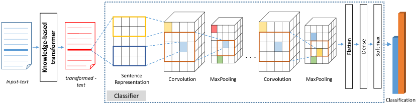
Figure 2. Model Architecture Diagram

We perform multiple experiments to test different BSW identification and bias mitigation strategies. We experiment with multiple classification methods like Logistic Regression, Multi-layer Perceptron (MLP), Convolutional Neural Network (CNN), an ensemble of classifiers. Since we obtained similar results irrespective of the classification method, we report results obtained using CNNs in this section.

We use identical Convolutional Neural Network (CNN) (Dixon et al., 2017) implemented in Keras (Chollet et al., 2015) for all the experiments. Fig. 2 shows the architecture diagram of the neural network. We use 100D GloVe (Pennington et al., 2014) embeddings to encode text and CNN architecture with 128 filters of size $5\times 5\times 5$ for each convolution layer, dropout of 0.3, max-sequence length as 250, categorical-cross-entropy as the loss function and RMSPROP as optimizer with learning-rate of 0.00005. We use the best parameter setting as described in Dixon et al. (2017) and train the classifiers for our task with batch size 128 and early stopping to a maximum of 20 epochs, keeping other hyperparameters constant throughout the experiments.

We use the spaCy  implementation of POS tagger and NER tool. More details about the experiments can be found in the source code .

5.4. Results

	ROC-AUC	$pAUC$
Biased	0.948	2.785
Wiki De-bias (Dixon et al., 2017)	0.957	1.699
NER tags	0.945	2.893
POS tags	0.958	1.053
K-Nearest Neighbour	0.910	3.480
WordNet - 0	0.943	2.781
WordNet - 1	0.949	2.530
WordNet - 2	0.958	1.634
WordNet - 3	0.954	2.068
WordNet - 4	0.951	2.390
WordNet - 5	0.954	1.992
Centroid Embedding	0.971	0.629

Table 5. Bias Mitigation Results using pAUC metric and ROC-AUC across Multiple Replacement Strategies on Wiki Madlibs Dataset. The best replacement strategy is highlighted in bold while the $2^{nd}$ best is underlined for each metric.

Detection Strategy $\rightarrow$	Manual List Creation				Skewed Occurrence Across Classes				Skewed Predicted Class Prob. Distribution
Replacement Strategy $\downarrow$	ROC-AUC	$PB_{mean}$	$PB_{sym}$	$PB_{asym}$	ROC-AUC	$PB_{mean}$	$PB_{sym}$	$PB_{asym}$	ROC-AUC	$PB_{mean}$	$PB_{sym}$	$PB_{asym}$
Biased	0.957	0.0806	0.1223	0.0144	0.952	0.1424	0.1473	0.0666	0.956	0.1826	0.2101	0.0505
Wiki Debias (Dixon et al., 2017)	0.958	0.0491	0.1433	0.0058	NA	NA	NA	NA	NA	NA	NA	NA
NE tags	0.956	0.0833	0.1269	0.0137	0.959	0.1741	0.2252	0.0421	0.955	0.1533	0.2118	0.0304
POS tags	0.953	0.0251	0.0540	0.0020	0.954	0.1614	0.2033	0.0481	0.958	0.0789	0.3656	0.0000
K-Nearest Neighbour	0.937	0.0554	0.1120	0.0023	0.936	0.1154	0.1196	0.0431	0.934	0.0618	0.1284	0.0035
Wordnet - 0	0.956	0.0765	0.1188	0.0121	0.946	0.1445	0.1620	0.0435	0.951	0.1835	0.2602	0.0283
Wordnet - 1	0.956	0.0756	0.1201	0.0133	0.954	0.1820	0.2132	0.0529	0.958	0.1191	0.3401	0.0002
Wordnet - 2	0.956	0.0735	0.1182	0.0110	0.952	0.1767	0.1986	0.0550	0.955	0.1453	0.3281	0.0037
Wordnet - 3	0.953	0.0708	0.1151	0.0098	0.941	0.1297	0.1622	0.0326	0.952	0.1699	0.3029	0.0121
Wordnet - 4	0.953	0.0733	0.1133	0.0097	0.946	0.1398	0.1570	0.0393	0.955	0.1751	0.3150	0.0123
Wordnet - 5	0.948	0.0653	0.1084	0.0057	0.959	0.1766	0.2336	0.0468	0.955	0.1561	0.3475	0.0060
Centroid Embedding	0.955	0.0000	0.0499	0.0000	0.953	0.1803	0.1918	0.0535	0.957	0.0774	0.1949	0.0000

Table 6. Hate Speech Detection Accuracy and Bias Mitigation Results Across Multiple Detection and Replacement Strategies on WikiDetox Dataset. The best replacement strategy is highlighted in bold while the $2^{nd}$ best is underlined for each metric.

5.4.1. BSWs identified by Various Strategies

Table 3 shows the list of BSWs obtained using different Bias Detection strategies. The words obtained from both the SOAC and SPCPD detection strategies are not obvious and differ from the manual set of words as the distribution of the terms in the training set can be arbitrary, motivating us to design detection strategies. In case of the Twitter Dataset, in Table 3, we do not show results for the ‘Manual List Creation’ detection strategy because we do not have a manual dataset of bias sensitive words for Twitter. The simple strategy of detecting biased words using Skewed Predicted Class Probability Distribution (SPCPD) is effective and works for arbitrary classifiers as well. The words obtained from the SPCPD detection strategy are not very obvious but the prediction on sentences that contain those words have very high discrepancy than expected prediction scores.

The BSWs obtained using the detection strategies are better than the ones obtained using the ‘Manual List Creation’ strategy because of the high $PB_{asym}$ scores for the ‘Biased’ classifier for different detection strategies as tabulated in Table 6. Additionally, the $PB_{asym}$ scores for BSWs from the manual list are very low in spite of a large number of words which suggests that the classifier is not biased towards these terms. For the Twitter dataset, the $PB_{asym}$ score for the SOAC detection strategy is the lowest, but in WikiDetox where the training dataset size is large, the skewness in distribution reduces resulting in the $PB_{asym}$ scores for the SPCPD detection strategy to be the lowest.

5.4.2. Effectiveness of various Bias Detection-Replacement Strategies

Tables 4, 5 and  6 show the hate speech detection accuracy and bias mitigation results across various bias detection and bias replacement strategies (averaged over 10 runs because of high variance) for the Twitter, Wiki Madlibs and WikiDetox datasets. ‘Biased’ replacement strategy indicates the biased classifier, i.e., the one where no bias has been removed. For Wiki De-bias bias removal strategy, we do not have results for non-manual detection strategies since they require template creation (like ‘Wiki Madlibs’) and dataset curation. We train the ‘Wiki De-bias’ (Dixon et al., 2017) baseline using the additional data containing 3,465 non-toxic samples as part of the dataset augmentation method as proposed in the original paper. For Wiki Madlibs dataset (Table 5), we show results using only manual list creation but across multiple bias replacement strategies, using $pAUC$ metric only since it is meant for this combination alone. WordNet-$i$ denotes the WordNet strategy where the starting synset level for finding hypernyms was set to $i$ levels up compared to the level of the bias sensitive word. For Tables 4 and  6, we use the ROC-AUC scores for comparing the general model performance while the $PB_{asym}$ metric for bias evaluation. We do not use $pAUC$ for these tables because they need manual generation of a dataset like Wiki Madlibs. Finally, note that the scores in the Table 4 and Table 6 are vertically grouped based on different detection strategies which involve varying set of BSWs making the results non-comparable across the detection strategies in general.

As seen in Table 5, for the Wiki Madlibs dataset, Centroid Embedding strategy performs the best beating the state-of-the-art technique (Wiki De-Bias) on both ROC-AUC as well as pAUC metrics. Additionally, POS tags and WordNet-based strategies also perform better than the Wiki De-bias strategy on the $pAUC$ metric with just a minor reduction in $ROC-AUC$ accuracy. The POS tags strategy performs better because the replaced words mostly belong to the same POS tag resulting in high generalization.

For the Twitter dataset, Centroid Embedding replacement method works best across all the detection strategies and across different metrics. The overall general classification performance for all the strategies remain almost similar, though the WordNet-3 replacement strategy works best. WordNet based replacement strategy is not as effective as the $PB_{asym}$ scores gradually increase with the increase in generalization, due to the absence of slang Twitter words in WordNet. The WordNet-based replacement strategies also show decreasing $PB_{asym}$ scores as the strategy is unable to find a suitable generalized concept that is already present in the Twitter dataset because of its small vocabulary size.

The WordNet and Centroid Embedding replacement strategies work best for the WikiDetox dataset. For the WordNet strategy, the best results vary based on detection strategy, but it performs either the best or gives comparable results to the best strategy. It also has an added benefit of deciding on the level of generalization which can be tweaked as per the task. For “manual list creation” detection strategy, Centroid Embedding provides unexpectedly low $PB$ scores because most of the words in the list are nouns. The non-zero $PB_{mean}$ metric in case of manual-list-creation detection strategy along with POS tags replacement strategy is due to the fact that the words like ‘gay’ are marked as Adjective instead of Noun, which is expected.

Finally, note that bias mitigation usually does not lead to any significant change in the ROC-AUC values, if performed strategically, while generally, it reduces bias in the learning.

5.4.3. Details of WordNet-based bias removal strategy

Table 7 shows WordNet-based replacement examples for the manual set of words with different values of the start synset level.

Original	Replaced Words
Word	Level 0	Level 1	Level 2	Level 3	Level 4	Level 5
sikh	disciple		follower	person	cause	entity
homosexual	homosexual	person	cause	entity		object
queer	faggot	homosexual		person	cause	entity
gay	homosexual	person	cause	entity		object
straight	homosexual	person	cause	collection	entity	object
muslim	person			cause	entity
deaf	deaf	people	group	abstraction	entity	-
latino	inhabitant			person	cause	entity

Table 7. WordNet based bias correction examples for the ‘Manual List Creation’ detection strategy with different start Synset Levels

Fig. 3 shows details about WordNet based replacement. As we traverse from right-to-left along the edges, we obtain generalizations for each of the words. The figure highlights two sets of similar words where one set (denoted by   ) is highly prone towards getting stereotypically biased, while all the highlighted terms (denoted by   ) represent “a group of people with specific attributes”. Each node represents the term which can be used for BSW replacement. In the case of multiple generalizations, the selection was made randomly.

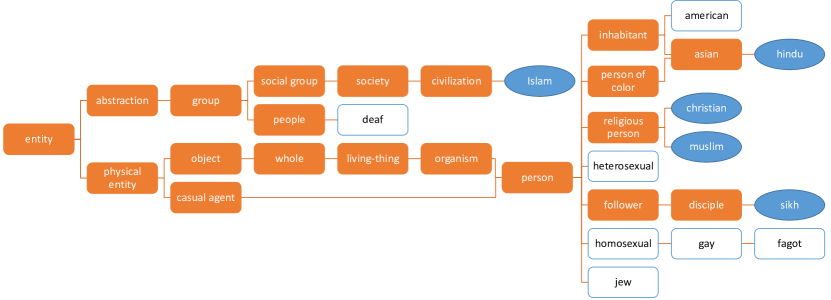
Figure 3. Horizontal representation of the WordNet Hypernym Hierarchy for BSWs.

Wordnet-based strategy often leads to the best results across our datasets. However, the results could be improved further using an appropriate normalization scale that captures generalization to different levels. For example, Hindu requires three levels of generalization, while Muslim requires two (see Fig. 3). This requires a generalization scheme that considers the inconsistency in the sibling nodes and performs differential normalization.

5.4.4. Case Studies

In order to evaluate the effectiveness of the Bias Detection strategy in identifying BSWs, we perform an experiment on a publicly accessible classifier, the Perspective API . We leverage the vocabulary of size 400k of GloVe vectors and obtain hate (toxicity) scores for each word in the vocabulary and rank them using the Skewed Predicted Class Probability Distribution Bias Detection strategy. This allows us to identify the set of bias sensitive words allowing us to create examples to test the quality of the obtained words. Some of these examples are tabulated in Table 1 where the API gives incorrect scores. The obtained examples show the effectiveness of the obtained BSWs.

Further, Table 8 shows some examples which were wrongly predicted as being “hateful” by the original ‘Biased’ classifier and the corresponding prediction scores after bias removal using the above strategies. These simple manually created examples clearly show the efficacy of our proposed method.

Examples	Toxicity
	Predictions
	before bias removal	after bias removal
are you a nerd ?	0.928	0.294
he hit the donkey	0.289	0.021
he is a gay	0.786	0.493
One of John brothers was homosexual while the other is a black transgender	0.690	0.048
katrina is a female african who is sikh	0.782	0.535

Table 8. Examples for predictions on sentences before and after the classifier had undergone the bias correction stage using the Centroid Embedding strategy for the manually constructed sentences containing identified BSWs. Bias Sensitive Words are marked in bold. The ideal prediction probabilities in all the cases should be less than 0.5

5.4.5. Unigrams versus higher order ngrams

In this paper, we experimented with unigrams only. From our experiments, we observed that the SB bias in unigrams propagates to word n-grams and char-n-grams as well. E.g., SB towards a word ‘women’ propagates to the char n-grams ‘wom, omen, wome’ as the distribution of char n-grams is similar to that of the corresponding word and also similar to the word n-grams, women are, womens suck, etc. Thus, considering unigrams is reasonably sufficient. That said, the PB metrics rely on the probability scores and thus can be easily used for bias sensitive n-grams as well.

6. Conclusions

In this paper, we discussed the problem of bias mitigation for the hate speech detection task. We proposed a two-stage framework to address the problem. We proposed various heuristics to detect bias sensitive words. We also proposed multiple novel knowledge generalization based strategies for bias sensitive word replacement which can be extended to other short-text classification tasks as well. Using two real-world datasets, we showed the efficacy of the proposed methods. We also empirically show that the data-correction based removal techniques can reduce the bias without reducing the overall model performance.

We also demonstrate the effectiveness of these strategies by performing the experiment on Google Perspective API and perform a qualitative analysis to support our observations using multiple examples.

References

- (1)
- Badjatiya et al. (2017) Pinkesh Badjatiya, Shashank Gupta, Manish Gupta, and Vasudeva Varma. 2017. Deep learning for hate speech detection in tweets. In Proceedings of the 26th International Conference on World Wide Web Companion. International World Wide Web Conferences Steering Committee, 759–760.
- Beutel et al. (2017) Alex Beutel, Jilin Chen, Zhe Zhao, and Ed H Chi. 2017. Data decisions and theoretical implications when adversarially learning fair representations. arXiv preprint arXiv:1707.00075 (2017).
- Blodgett and O’Connor (2017) Su Lin Blodgett and Brendan O’Connor. 2017. Racial Disparity in Natural Language Processing: A Case Study of Social Media African-American English. arXiv preprint arXiv:1707.00061 (2017).
- Bolukbasi et al. (2016) Tolga Bolukbasi, Kai-Wei Chang, James Y Zou, Venkatesh Saligrama, and Adam T Kalai. 2016. Man is to computer programmer as woman is to homemaker? debiasing word embeddings. In Advances in Neural Information Processing Systems. 4349–4357.
- Caliskan et al. (2017) Aylin Caliskan, Joanna J Bryson, and Arvind Narayanan. 2017. Semantics derived automatically from language corpora contain human-like biases. Science 356, 6334 (2017), 183–186.
- Chollet et al. (2015) François Chollet et al. 2015. Keras. https://keras.io.
- Davidson et al. (2017) Thomas Davidson, Dana Warmsley, Michael Macy, and Ingmar Weber. 2017. Automated Hate Speech Detection and the Problem of Offensive Language. (2017).
- Dixon et al. (2017) Lucas Dixon, John Li, Jeffrey Sorensen, Nithum Thain, and Lucy Vasserman. 2017. Measuring and Mitigating Unintended Bias in Text Classification. (2017).
- Djuric et al. (2015) Nemanja Djuric, Jing Zhou, Robin Morris, Mihajlo Grbovic, Vladan Radosavljevic, and Narayan Bhamidipati. 2015. Hate Speech Detection with Comment Embeddings. In Proceedings of the 24th International Conference on World Wide Web (WWW ’15 Companion). ACM, New York, NY, USA, 29–30. https://doi.org/10.1145/2740908.2742760
- Feldman et al. (2015) Michael Feldman, Sorelle A Friedler, John Moeller, Carlos Scheidegger, and Suresh Venkatasubramanian. 2015. Certifying and removing disparate impact. In Proceedings of the 21th ACM SIGKDD International Conference on Knowledge Discovery and Data Mining. ACM, 259–268.
- Friedler et al. (2016) Sorelle A Friedler, Carlos Scheidegger, and Suresh Venkatasubramanian. 2016. On the (im) possibility of fairness. arXiv preprint arXiv:1609.07236 (2016).
- Hardt et al. (2016) Moritz Hardt, Eric Price, Nati Srebro, et al. 2016. Equality of opportunity in supervised learning. In Advances in neural information processing systems. 3315–3323.
- Hovy and Spruit (2016) Dirk Hovy and Shannon L Spruit. 2016. The social impact of natural language processing. In Proceedings of the 54th Annual Meeting of the Association for Computational Linguistics (Volume 2: Short Papers), Vol. 2. 591–598.
- Khosla et al. (2012) Aditya Khosla, Tinghui Zhou, Tomasz Malisiewicz, Alexei A Efros, and Antonio Torralba. 2012. Undoing the damage of dataset bias. In European Conference on Computer Vision. Springer, 158–171.
- Kleinberg et al. (2016) Jon Kleinberg, Sendhil Mullainathan, and Manish Raghavan. 2016. Inherent trade-offs in the fair determination of risk scores. arXiv preprint arXiv:1609.05807 (2016).
- Kwok and Wang (2013) Irene Kwok and Yuzhou Wang. 2013. Locate the Hate: Detecting Tweets against Blacks.. In AAAI.
- Miller (1995) George A. Miller. 1995. WordNet: A Lexical Database for English. Commun. ACM 38, 11 (Nov. 1995), 39–41. https://doi.org/10.1145/219717.219748
- Olteanu et al. (2018) Alexandra Olteanu, Emre Kiciman, and Carlos Castillo. 2018. A Critical Review of Online Social Data: Biases, Methodological Pitfalls, and Ethical Boundaries. In Proceedings of the Eleventh ACM International Conference on Web Search and Data Mining (WSDM ’18). ACM, New York, NY, USA, 785–786. https://doi.org/10.1145/3159652.3162004
- Pennington et al. (2014) Jeffrey Pennington, Richard Socher, and Christopher Manning. 2014. Glove: Global vectors for word representation. In Proceedings of the 2014 conference on empirical methods in natural language processing (EMNLP). 1532–1543.
- Tatman (2017) Rachael Tatman. 2017. Gender and Dialect Bias in YouTube’s Automatic Captions. In Proceedings of the First ACL Workshop on Ethics in Natural Language Processing. 53–59.
- Waseem and Hovy (2016) Zeerak Waseem and Dirk Hovy. 2016. Hateful symbols or hateful people? predictive features for hate speech detection on twitter. In Proceedings of the NAACL student research workshop. 88–93.
- Wulczyn et al. (2017) Ellery Wulczyn, Nithum Thain, and Lucas Dixon. 2017. Ex machina: Personal attacks seen at scale. In Proceedings of the 26th International Conference on World Wide Web. International World Wide Web Conferences Steering Committee, 1391–1399.