Correlation-induced steady states and limit cycles in driven dissipative quantum systems
Abstract
We study a driven-dissipative model of spins one-half (qubits) on a lattice with nearest-neighbor interactions. Focusing on the role of spatially extended spin-spin correlations in determining the phases of the system, we characterize the spatial structure of the correlations in the steady state, as well as their temporal dynamics. In dimension one we use essentially exact matrix-product-operator simulations on large systems, and pushing these calculations to dimension two, we obtain accurate results on small cylinders. We also employ an approximation scheme based on solving the dynamics of the mean field dressed by the feedback of quantum fluctuations at leading order. This approach allows us to study the effect of correlations in large lattices with over one hundred thousand spins, as the spatial dimension is increased up to five. In dimension two and higher we find two new states that are stabilized by quantum correlations and do not exist in the mean-field limit of the model. One of these is a steady state with mean magnetization values that lie between the two bistable mean-field values, and whose correlation functions have properties reminiscent of both. The correlation length of the new phase diverges at a critical point, beyond which we find emerging a new limit cycle state with the magnetization and correlators oscillating periodically in time.
I Introduction
Atomic, optical, and solid-state systems are often operated in many-body nonequilibrium regimes characterized by a competition between interactions, nonlinearity, coherent external driving and dissipative dynamics. These include arrays of coupled circuit quantum electrodynamic (QED) units Houck et al. (2012), spin ensembles embedded into large optical or microwave cavities Kubo et al. (2010); Grezes et al. (2014); Fink et al. (2017), mesoscopic quantum circuits of increasing complexity interfaced with microwave resonators Bruhat et al. (2016); Parlavecchio et al. (2015), trapped ions Bohnet et al. (2016) and cold atoms Diehl et al. (2010); Keeling et al. (2010). A rich pattern of behaviors at the interface between quantum optics and condensed matter physics is observed with systems of strong light-matter interactions Chang et al. (2008); Bhaseen et al. (2012); Otterbach et al. (2013); Höning et al. (2013); Carusotto and Ciuti (2013); Ritsch et al. (2013, 2013); Schmidt and Koch (2013); Le Hur et al. (2016); Noh and Angelakis (2017); Hartmann (2016); Schiró et al. (2016). Dissipative phase transitions and critical phenomena in open systems attract increasing attention and research activity Greentree et al. (2006); Hartmann et al. (2006); Nagy et al. (2011); Öztop et al. (2012); Schiró et al. (2012, 2013); Torre et al. (2013); Kulkarni et al. (2013); Brennecke et al. (2013); Schiró et al. (2016); Fitzpatrick et al. (2017); Scarlatella et al. (2019); Ma et al. (2019); Marino and Diehl (2016); Shchadilova et al. (2020); Kirton et al. (2019); Sánchez Muñoz et al. (2019); Munoz et al. (2019). Driving and dissipation can be utilized in the generation of topological quantum states by coupling to a specially tailored bath Bardyn et al. (2013) or time-periodic (Floquet) driving Oka and Kitamura (2019). Proposals to realize artificial gauge fields with circuit-QED photonic lattices Koch et al. (2010), chiral edge modes Petrescu et al. (2012); Hafezi et al. (2013a) and quantum Hall fluids of light Cho et al. (2008); Umucalılar and Carusotto (2011); Hafezi et al. (2013b), follow the paradigm of engineering topological states in fully neutral quantum systems Rechtsman et al. (2013).
An open quantum system coupled to a Markovian bath obeys a Lindblad master equation for the time evolution of the density matrix ,
| (1) |
Here the first term on the right-hand side describes the coherent evolution due to interactions and possibly coherent driving terms (with the Hamiltonian in the rotating frame), while the dissipator accounts for dephasing and relaxation processes due to the environment, described by a set of jump operators. The simplest approach for obtaining solutions of such systems, applied to various driven-dissipative systems (mostly of coupled spins or oscillators) Lee et al. (2011); Qian et al. (2012); Jin et al. (2013, 2014); Schiró et al. (2016); Parmee and Cooper (2018); Foss-Feig et al. (2017); Biondi et al. (2017a); Chan et al. (2015); Wilson et al. (2016); Marcuzzi et al. (2014), is the mean-field (MF) decoupling limit, in which is approximated by a product of single-site density matrices. The MF phase diagrams obtained this way manifest both translationally-invariant steady states and antiferromagnetic (AF) or staggered phases of a spontaneously broken symmetry, where neighbouring sites have different mean magnetization or density. Oscillatory limit cycle (LC) phases that break time-translation invariance Iemini et al. (2018) have also been found, and in addition, there are bistable or multistable parameter regions where two or more different states coexist.
A highly debated question in the literature is whether the AF, LC, and multistable phases found in MF are genuine features of the quantum system.
A large number of studies concern one-dimensional (1D) lattices (mostly with nearest-neighbor interactions), finding that the MF AF phase is replaced by a uniform phase stabilized by AF correlations Lee et al. (2011); Wilson et al. (2016); Biondi et al. (2017b, 2018), and bistability is replaced by a smooth crossover accompanied by large quantum fluctuations Weimer (2015); Mendoza-Arenas et al. (2016); Foss-Feig et al. (2017); Vicentini et al. (2018); Landa et al. (2020). These conclusions rely on accurate numerical methods that can be applied to large 1D systems, such as matrix product operator (MPO) simulations, but an experimental investigation is still lacking. In two-dimensional (2D) lattices, numerical methods are much more limited. MF bistability has been found by some approximate methods to be replaced by a sharp first order jump between two phases Foss-Feig et al. (2017); Vicentini et al. (2018); Weimer (2015); Jin et al. (2018); Kshetrimayum et al. (2017). A dynamical timescale diverging at the jump has been found Weimer (2015); Vicentini et al. (2018); Landa et al. (2020), which is attributed to a vanishing Liouvillian gap – the smallest magnitude of the real part of the nonzero eigenvalues Minganti et al. (2018). Limit cycles in the driven-dissipative Heisenberg lattice which are predicted in MF, were found to disappear due to short-range correlations in finite dimensions Owen et al. (2018).
In Landa et al. (2020) we have presented a theoretical scenario for quantum bistability in driven dissipative lattice systems of spatial dimension two and higher. We have provided numerical evidence in its support using a self-consistent theory of quantum fluctuations beyond mean field, dubbed MF with quantum fluctuations (MFQF) and MPO simulations, applied to spins one-half. Within this scenario the MF bistability is not washed away by quantum correlations, provided the thermodynamic limit of infinite large system size is taken before the long-time limit, i.e. provided the system is studied on time scales which are smaller than exponential in system size. We also discussed what this scenario implies concerning the slowly-relaxing eigenstates of the Liouvillian super operator.
The questions we address in this work are: (i) How the patterns of stationary states and fixed point of the dissipative dynamics change with increasing interactions in the system, and in particular how they deviate from the MF solutions, (ii) whether phases not accessible in MF can be induced and stabilized in the system by the quantum correlations, and (iii) whether long-range (spatial and temporal) order induced by a competition between driving and dissipation can be stabilized by quantum fluctuations beyond MF. Specifically, we consider a driven-dissipative quantum spin model, discussed in Landa et al. (2020). We study its steady state and dynamical properties for larger values of the nearest-neighbor interactions (as compared to the regime studied in Landa et al. (2020)), presenting for completeness and as a reference point, a detailed study of the MF limit. In dimension two and higher we find two new states that are stabilized by quantum correlations and do not exist in the MF limit of the model. One of these is a steady state with mean magnetization values that lie between the two bistable MF values, and whose correlation functions have properties reminiscent of both. The correlation length of the new phase diverges at a critical point, beyond which we find emerging a new limit cycle state with the magnetization and correlators oscillating periodically in time.
The paper is organized as follows. In Sec. II we present a summary of the main results of the paper. In Sec. III we present the equations of motion which form the starting point for calculating the dynamics of observables within the MF and MFQF approaches, presenting details of the MF limit in Sec. IV. In Sec. V.1 we discuss the MFQF approximation scheme that goes beyond MF, and in Sec. V.2 we describe a method based on matrix product operators (MPO), applied to the present model in 1D and 2D. In Sec. VI we present our results obtained using MPO and MFQF, and in Sec. VII we conclude with a summary and outlook. The Appendix contains some further details of the theory and numerics.
II Main Results
We study a driven-dissipative model on a hypercubic lattice in dimensions, with sites located at , and connectivity . We consider spins one-half using the Pauli matrices at each site, with , and the ladder operators . Decomposing the Hamiltonian into the kinetic (hopping) part and the sum of on-site terms, we have
| (2) |
where describes two-level quantum systems driven with amplitude and detuning , in a frame rotating with the drive, using the rotating wave approximation, as derived in App. E. Here, is
| (3) |
with the summation extending over all lattice bonds. Setting we have a dissipative Ising model, introduced in Lee et al. (2011). In this summary section we set , focusing on the driven-dissipative XY model, first considered in Mendoza-Arenas et al. (2016); Wilson et al. (2016). For independent couplings with rate of each site to a zero-temperature bath, the dissipator in Eq. (1) reads
| (4) |
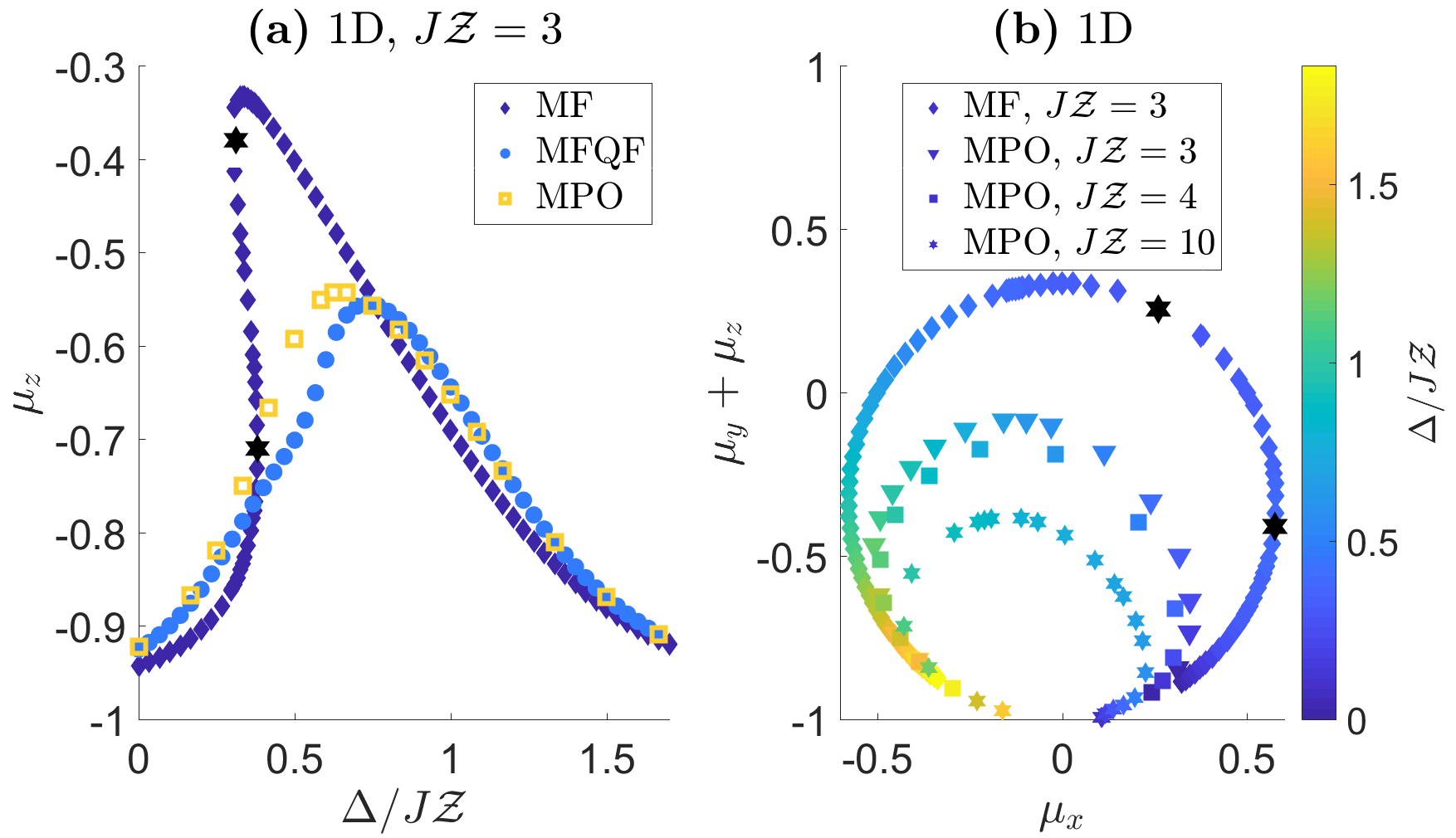
Assuming a translationally invariant state (further discussed in Sec. III), we define the time-dependent mean magnetization and its steady-state value (assuming it exists) as
| (5) |
As shown in Sec. IV.1, the steady-state magnetization lies in the plane that for and becomes , which can be spanned by the two (orthogonal) vectors and . This is an exact result that requires only translation-invariance.
In MF, is further constrained to lie on the circumference of an ellipse. Figure 1 depicts the MF trajectory of in the steady state plane for as a function of (with this rescaling facilitating comparison at different interaction strengths discussed in the following). As seen in Fig. 1(a), for there is a single solution with and . Increasing , this solution moves counter-clockwise along the MF ellipse [Fig. 1(b)]. At , a new stable solution appears at a high value, together with an unstable solution. As is increased, the new stable solution moves counter-clockwise along the MF ellipse while the unstable solution moves clockwise, until at , the unstable solution collides with the first stable solution, both becoming complex and hence ceasing to be physical solutions. The remaining single solution continues along the ellipse towards as .
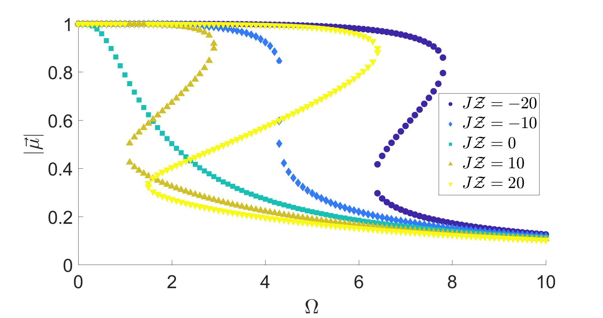
In the presence of correlations, the magnetization departs from the MF ellipse (but remains in the plane). MPO calculations in 1D with up to a few hundred sites (and the results verified for convergence with ) show a significant deviation from MF for , with a smooth crossover between the two limiting regimes. This crossover can be seen in Fig. 1(a) [for ], showing also that the MFQF approximation is capable of washing away the bistability region resulting in a single phase that follows approximately the numerically exact MPO solution. This result has been discussed in Landa et al. (2020) for a somewhat higher value of (and identical values of the other parameters). We attribute this capability of MFQF to the fact that it incorporates correlations with a nontrivial spatial dependence, which is an important characteristic of the many-body solution. As shown in Landa et al. (2020), in the heart of the crossover region the correlations grow by up to a few orders of magnitude. The strength of the correlations depends naturally on the interaction coefficient , and in Fig. 1(b) it can be seen that, as is increased, the trajectory of deviates further from the MF ellipse, due to the correlators increasing in magnitude. In Sec. VI we present a detailed comparison of the MFQF and MPO solutions in 1D for a larger value (), and discuss the similarities and deviations observed.
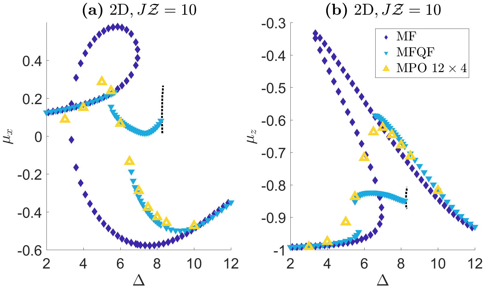
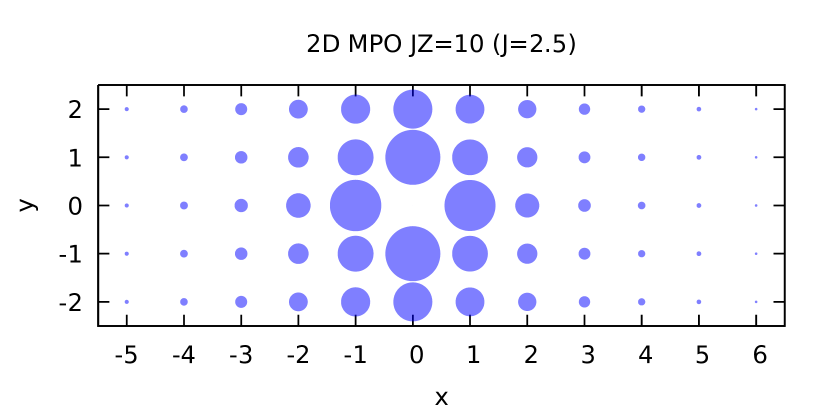
Turning to 2D lattices, Fig. 2 shows the magnetization of the MF and MFQF steady states for strong interactions (, and , ) on a 2D lattice with periodic boundary conditions, and the MPO steady state on a cylinder of length and circumference . The MPO mean magnetization coincides quantitatively very well with that of MFQF (simulating a 2D lattice of up to sites), for the steady state on the branch coming from high down to . This is a regime where the correlation length is not large (of order lattice sites). The steady state on the cylinder appears to be locally very close to that of a large system. This is evidenced by the correlation functions, and Fig. 3 depicts the connected two-point correlation function [defined in Eq. (13)], calculated in MPO. We see that the nearest-neighbour correlations are nearly isotropic, and along the cylinder’s symmetry axis the correlations decay rapidly. However, for MFQF predicts bistability in the thermodynamic limit, while due to the finite size of the MPO cylinder, the MPO steady state is necessarily unique, and must depend smoothly on . We can therefore not expect these finite-size MPO calculations to show bistability or even a discontinuity. At low values incommensurate spin-spin correlations develop (with a long correlation length, although with a relatively small magnitude). There, the MPO simulations are affected by the small size of the cylinder, and the agreement with MFQF is only semi-quantitative.
In addition to the possibility of the coexistence of stable MF-like branches, in MFQF a new branch appears in some range of , as shown in Fig. 2. The mean magnetization on this branch has intermediate values between the two MF-like branches. The new intermediate branch has large and spatially modulated two-point correlations, whose characteristics are shown in detail in Fig. 17 in Sec. VI. Moreover, we find that at the high- edge of the branch the correlation length diverges (in practice, reaches the linear size of the lattice). Beyond this point, we find a small range of values for which an oscillatory LC state is stabilized by large correlations extending throughout the lattice. This phenomenon is not present in the MF approximation. The oscillation patterns of the mean magnetization and two-point correlation functions are presented in Sec. VI.
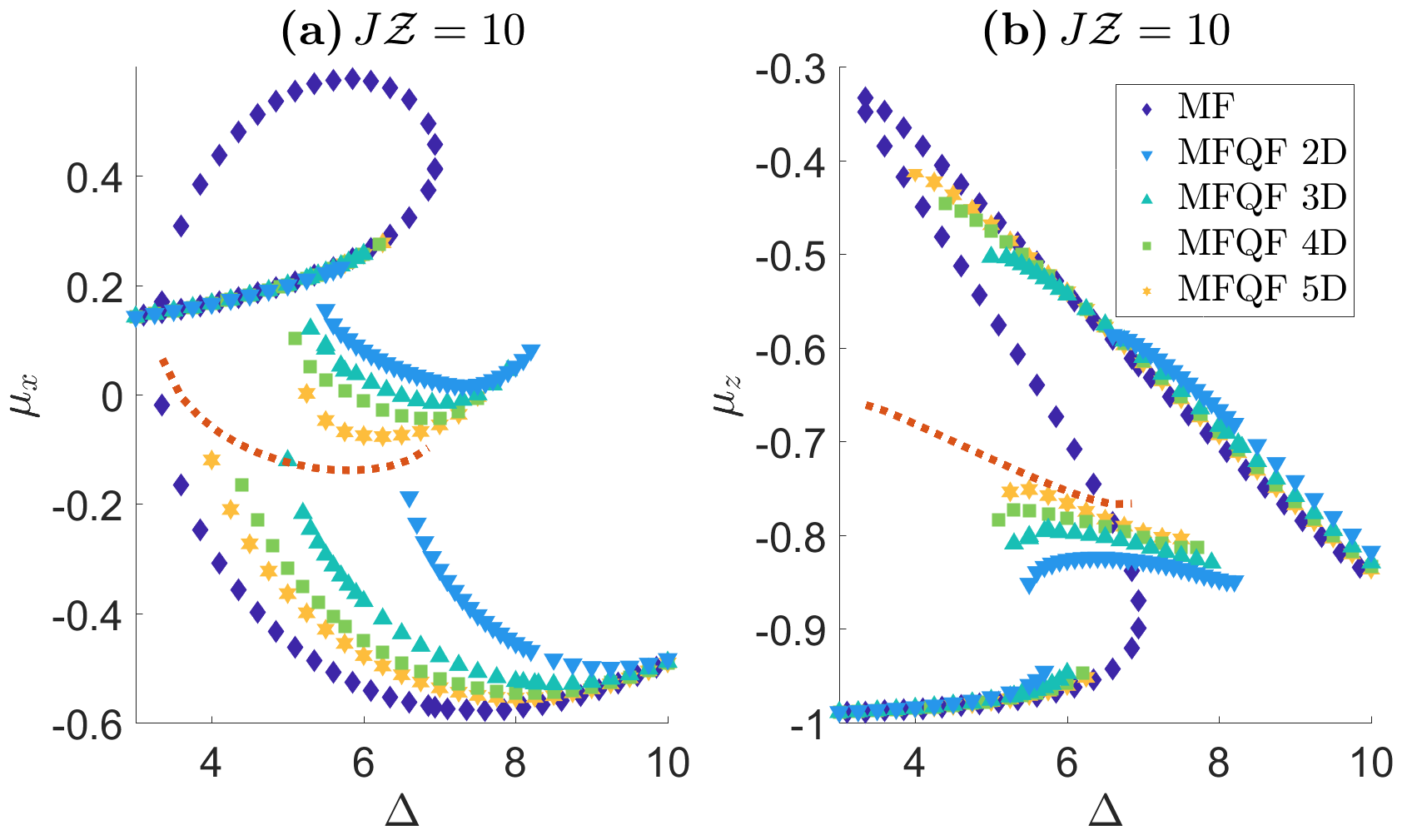
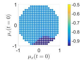
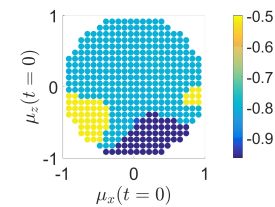
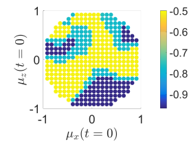
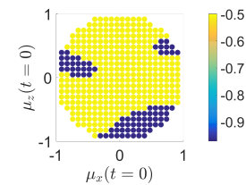
The MFQF approximation is easy to apply in higher dimensions, and the dynamics can be solved with a very large number of spins. Figure 4 shows the results of such simulations carried out with large lattices from 2D through 5D. We find multistable branches in progressively larger ranges of , which converge towards the MF bistability region. At the same time, the range of the intermediate branch is slowly shrinking as is increased. We thus see how the MFQF solutions gradually approach the MF ones when is increased. For the steady state we present in Fig. 5 a look into the basins of attraction of the coexisting multistable steady-states. The basins of attraction, whose construction starting from initial product states is explained in more detail in Sec. IV.2, are taken at fixed values of the parameters, varying only . We see that, as is increased from 2 to 4, the basin of attraction of the new branch shrinks and gives way to increasingly MF-like basins for the two MF states.
Our study proposes some answers to the questions posed in the outset. Briefly, our study suggests that quantum phases in presence of driving and dissipation can support large fluctuations, depending on the dimension and interaction strength, and that a behaviour commonly associated with classical nonlinearity – namely bistability and hysteresis – is effectively possible in the thermodynamic limit of the studied quantum system in 2D and above. We find new emerging states of the system in the long time limit, phases not accessible in MF, which are induced and stabilized by quantum fluctuations and correlations. For critical parameters long-range spatial order can be sustained in the lattice due to the competition of the drive, dissipation and interactions, and for some parameter ranges, also a temporal order in the form of a spontaneous forming of a stable limit cycle. Whether these phases survive as true solutions of the full quantum system remains a fundamental open question, possibly awaiting for experimental quantum simulation for full confirmation. Experiments are foreseeable with trapped ions and superconducting qubits, and can possibly answer general questions about the dynamics of many-body quantum systems, beyond the sizes accessible to state-of-the-art numerics.
III Equations of Motion
In this section we present the equations of motion (e.o.m) for observables of the quantum system Sandri et al. (2012), which form the basis for the MF and MFQF approaches. We define -points expectation values in the form
| (6) |
By multiplying Eq. (1) with an operator and taking the trace, we get an e.o.m for the expectation value
| (7) |
Starting with single-site operators , this leads to a hierarchy of equations that depend on the value of correlators at the next order, . A simple way to handle the derivation is to use the linearity of the equation and treat separately the Hamiltonian and the dissipative parts. Matrix elements do not depend on the picture by which they are calculated, and in the following we calculate the Hamiltonian part of the e.o.m in the Heisenberg picture, and the dissipative part in the Schrödinger picture.
An Heisenberg e.o.m for any operator reads in the absence of dissipation,
| (8) |
and using the commutation relations of App. B we obtain the Heisenberg e.o.m (for ),
| (10) |
with the summation of extending over the nearest neighbours of the lattice site .
We now assume that the initial density matrix commutes with spatial translations and reflection. In this case, with a Hamiltonian that is also invariant under these operations, the time evolution will remain in the same symmetry sector, which is characterized by a uniform magnetization, and two-point correlations that are only a function of the distances. This precludes the possibility of spontaneous symmetry breaking in the thermodynamic limit, however for no AF phase is expected based on MF and 1D MPO results. In addition, we did not observe any sign of modulation instability of the uniform states. We (re-)define the MF magnetization of Eq. (5),
| (11) |
and we define a two-point correlation function (correlator),
| (12) |
which is a function of the difference alone, symmetric in (because and commute). The connected two-point correlator is defined (for ) by
| (13) |
We will similarly refer to the connected three-point correlator defined for ,
| (14) |
which is again a function of the differences only.
Substituting the definition of the correlators in Eqs. (III)-(10), taking the expectation value and including the dissipative terms obtained by calculating in the Schrödinger picture as in Eq. (7), we get the e.o.m
| (15) | |||||
| (16) | |||||
| (17) |
where is the correlator at distance (with the norm on the -dimensional cubic lattice). We write explicitly
| (18) |
Eqs. (15)-(17) are exact, but do not form a closed system. In the following sections we study the MF and MFQF approximations, obtained by closing the equations by truncation at different orders of -point correlations. For a related approach based on expansion of the density matrix in the inverse connectivity, see Biondi et al. (2017b).
IV Mean field
IV.1 The mean-field steady state
Setting in Eqs. (15)-(17), which amounts to assuming that the density matrix is a product of identical on-site states, we get the MF e.o.m,
| (19) | |||
| (20) | |||
| (21) |
where we have set ; Since the MF equations depend only on the difference , the MF results for the XY model hold equally well for the Ising model (by the replacement ), and equivalently, for any combination of the two interaction types (this equivalence ceases to hold when correlations beyond MF are considered). Combining Eqs. (19)-(21), the squared length of the MF spin evolves according to
| (22) |
where the r.h.s is always negative for magnetization within the unit sphere. The MF equations are invariant under two different discrete symmetries
| (23) |
and
| (24) |
These two symmetries manifest themselves in the parameter-space dependence of the steady state as discussed below.
Setting the time-derivative of Eqs. (19)-(21) to zero and isolating , its steady-state value is determined through a third order polynomial equation, which can have either one real root (and two complex conjugate roots), or three real ones. Each root of the polynomial gives a solution for , from which we get immediately the corresponding and . In the case of three different real roots, there are two stable solutions and one unstable solution, as we find from a linear stability analysis; linearizing the e.o.m about any steady-state solution by substituting
| (25) |
we obtain a linear system for the small fluctuations which is defined by the matrix
| (26) |
and is linearly stable to uniform perturbations when all eigenvalues of this matrix have a nonpositive real part.
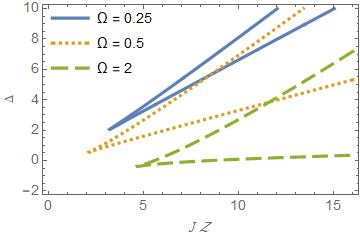
We note that the limit of is singular, because for there is no steady-state and the dynamics become Hamiltonian. We present all results by setting , which defines the units of energy and time. The condition for bistability is that the discriminant of the cubic equation of the magnetization is positive. As a function of the parameters, the discriminant is a high order polynomial, and the condition of its positivity defines a 3D region in parameter space, at fixed value of . This region has disconnected components related by the symmetries of Eqs. (23)-(24). We find that bistability requires (see below). For any fixed there is a bistability region in the -plane on each side of the line , starting at a cusp point from which two curves emanate defining the bistability boundary, see Fig. 6. On each (bifurcation) curve the unstable solution coincides with one stable solution, and both solutions lead to a zero eigenvalue upon linearization, with the same eigenvector. At the cusp the three MF solutions coincide and each has a zero eigenvalue, all with the same eigenvector. The cusp is also a critical point where an effective symmetry appears, as discussed in Marcuzzi et al. (2014).
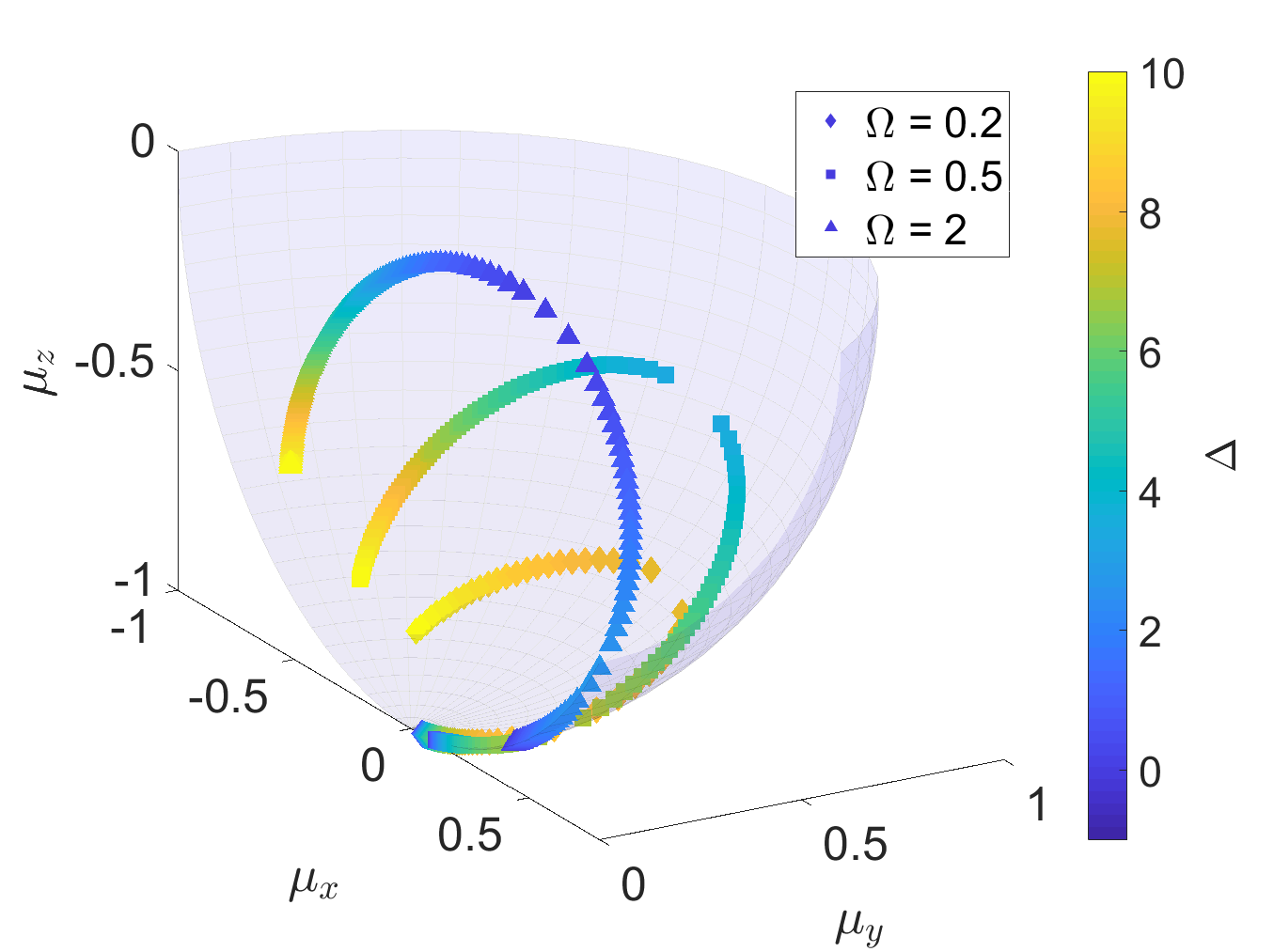
However, not all values of are allowed in the steady state. Using Eq. (22), the mean magnetization vector in the steady state is constrained to lie on the surface of the ellipsoid
| (27) |
which is centered about and has a principal semi-axis of length , going from the infinite temperature solution point at to the pure (product) state at , so that at the steady state the solution obeys . Using Eq. (21), the steady state at a fixed value of is obtained by the intersection of the ellipsoid of Eq. (27) with the plane
| (28) |
which also shows that is related to by a displacement and stretching, and that the sign of is equal to the sign of . For the steady state is the pure product state , while for for (with the other parameters fixed), we have found that the steady state is the infinite temperature state, .
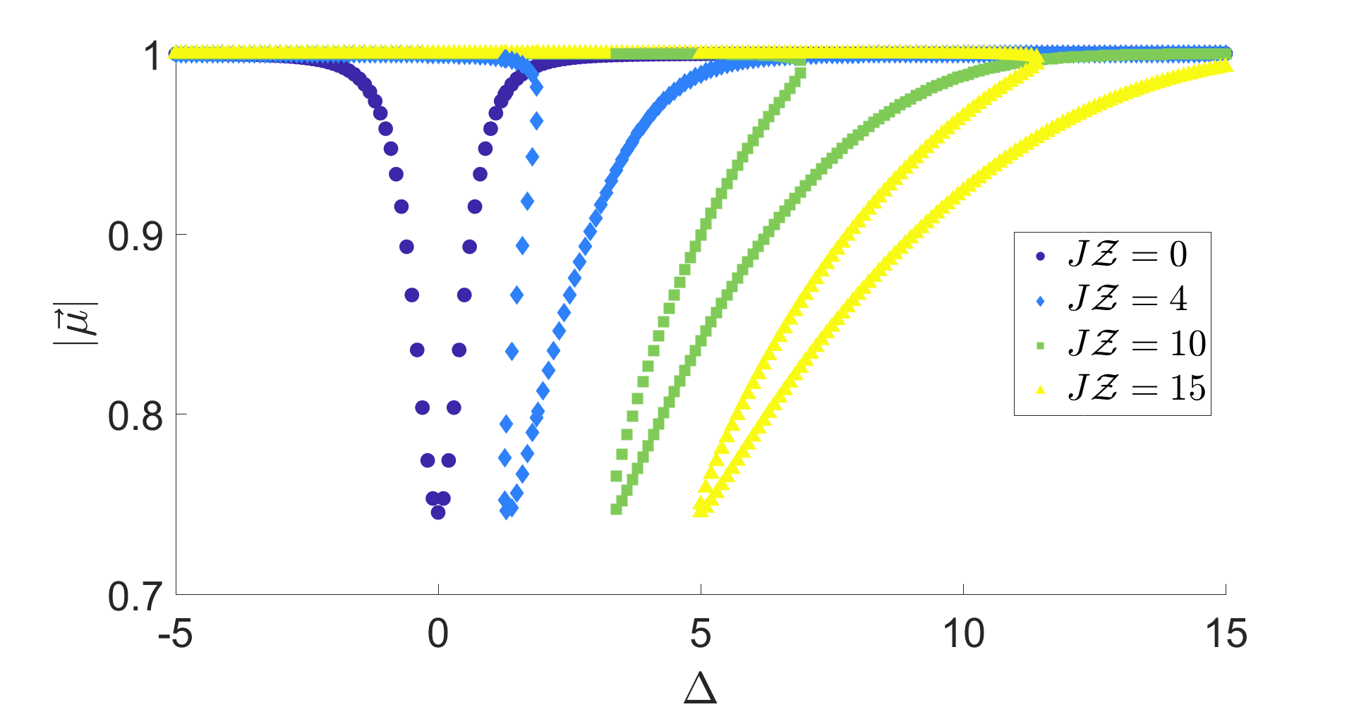
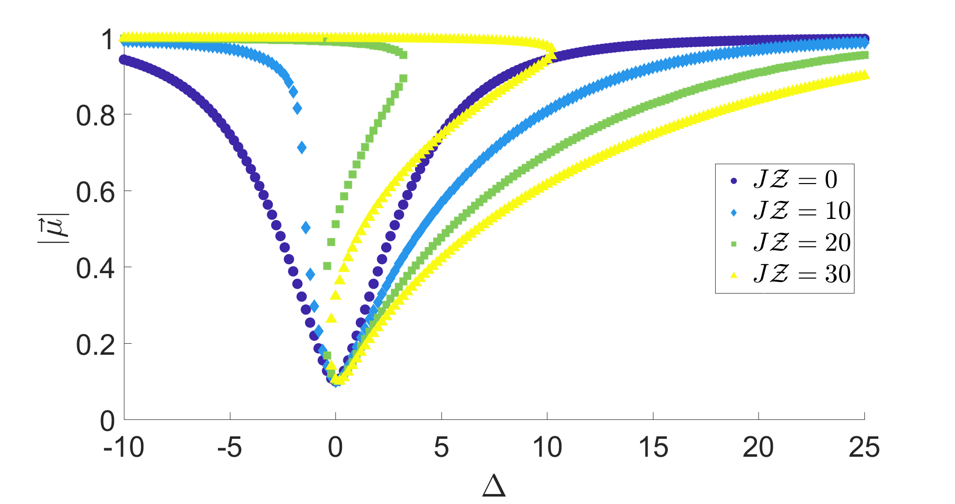
Figure 7 shows how the three components of the mean-field magnetization vary with for fixed and three values (0.2, 0.5 and 2) of . The ellipsoid of Eq. (27) is visible, as well as the fact that the magnetization vector must lie in a plane determined by Eq. (28). Pairs of points (on the same ellipsoid) with the same color (i.e. same ) are the bistable solutions. However, as this is hard to discern in this figure, Figs. 8-10 present as a function of some of the model parameters, exemplifying the limits of , the bistability, and its dependence on the parameters. Some further properties of the MF steady state are derived in App. A.
IV.2 Mean-field dynamics
We now turn to the dynamics associated to the MF e.o.m. We here focus on one property of the dynamical system, which is the distribution of initial conditions converging to the possible steady states for parameters in the bistability region. The basins of attraction of each of the bistable solutions can be calculated by starting the dynamics at initial conditions chosen within the unit magnetization sphere , and following the dynamics to the steady state. The basins of attraction contain information on the global dynamics and were presented in Fig. 5 of Sec. II using the MFQF approach.
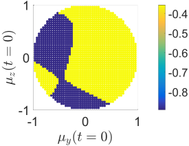
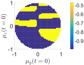
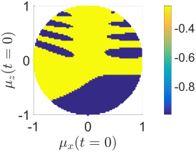
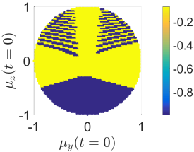
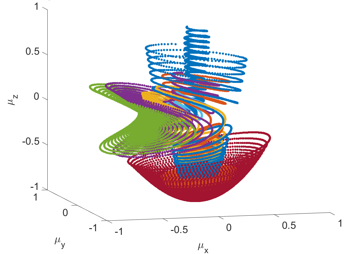
In order to visualize the basins of attraction we consider transversal cuts through the state-space, i.e. by restricting the initial conditions to a plane, e.g. . We find that other planar cuts appear qualitatively similar (as exemplified in Fig. 11); we plot in Fig. 11 (given by the color code), as a function of the initial condition . As can be seen, the basins in the region are stretched and twisted into each other as the parameters are increased into the weak damping limit (for which ). A quantification of the mixing of the basins of attraction could be done by measuring the length of the boundary curve between the two basins, or perhaps just by counting the number of jumps on the boundary of the circle. A more detailed investigation of the dynamics would be required in order to explain this mechanism. However, Fig. 12, showing the dynamics of in the weak damping limit, suggests an initial understanding. It can be seen that many rotations in phase space take place before the solution settles to one of the steady states, with neighbouring initial conditions originating from the upper half of the Bloch sphere separating into the two steady states. Clearly, at weak , the combined effects of fast precession with the bistability of the final state gives the MF dynamics some strong sensitivity to the initial condition.
V Approaches going beyond mean field
In this section we present two methods allowing to explore the physics of the model beyond the MF approximation. The first (Sec. V.1), MFQF, amounts to dress the MF state at leading order by two-point correlations. Next, in Sec. V.2, we describe a numerical method based on MPO which allows for a controlled and accurate approach to the true many-body state in low dimension (1D and thin 2D cylinders). The results obtained by these two complementary techniques will be compared and discussed in Sec. VI.
V.1 Mean field with Quantum Fluctuations
Going beyond MF, the next order correction can be included by deriving the e.o.m of [setting ]. The approximation we present is based on assuming that , defined in Eq. (14), and higher order connected correlators, can be neglected in comparison to . The e.o.m of is
| (29) |
where the local Hamiltonian terms are described using the matrix
| (30) |
while , which contains terms proportional to and to , comes from the kinetic terms, and comes from the Lindbladian part. Both are derived in App. B. By using Eq. (13) we get the e.o.m system for ,
| (31) |
which we solve numerically together with the coupled system for [Eqs. (15)-(17)], on lattices of varying sizes, surpassing one hundred thousand sites.
We consider the covariance matrix of the total magnetization,
| (32) |
whence the imaginary term drops from the symmetrized covariance per spin, which has a finite nontrivial value in the thermodynamic limit ,
| (33) |
The first terms result from the local properties of the spin-one-half system. In the following we will study the total (connected) correlation as a measure of the correlations in a fluctuating domain,
| (34) |
V.2 Matrix product operators
We numerically solve the Lindblad equation using an MPO representation of the density matrix of the system Zwolak and Vidal (2004); Verstraete et al. (2004); Prosen and Žnidarič (2009); Benenti et al. (2009); Mascarenhas et al. (2015). Since the density matrix can be considered as a pure state (i.e. a wave function) in some enlarged Hilbert space with four states per sites, it can be encoded as an matrix-product state (MPS) in that enlarged space. In this vectorized representation, the density matrix is often noted , as a “super ket”. This point of view allows to implement the Lindblad evolution in a way that is formally similar to the unitary evolution of a pure state in tDMRG, the Hamiltonian being replaced by the Lindbladian (super)operator.
One qualitative difference with the unitary evolution is of course the fact that the “norm” is not conserved during the time evolution. The latter is simply related to the second Rényi entropy of the system, . If we denote by the super ket representing the identity density matrix, the scalar product is, however, conserved. In addition, in presence of dissipation, a finite-system is expected to have a unique steady-state, independent of the initial conditions (note that this may no longer be true if one first takes the thermodynamic limit and then the limit of long times Landa et al. (2020)).
As for MPS-based methods describing pure states, an MPO-based description of a mixed state gets more and more precise as the so-called bond dimension is increased. In 1D, we expect that (in generic situations) the bond dimension required to achieve a given precision does not grow with the system size (like when encoding a gapped pure state with MPS). For this reason one can access long times and very accurate results for large 1D systems.
In the same way as MPS methods can be used for 2D lattices, using a snakelike path visiting all sites Stoudenmire and White (2012), one can encode the density matrix of a 2D mixed state using an MPO. One price to pay is the fact that interactions that are local in 2D become long-ranged along the one-dimensional path. For this approach the most natural geometry is that of a cylinder, with open boundary conditions in the direction, and periodic ones in the direction. In that case the bond dimension required to achieve a given precision grows exponentially with the cylinder diameter , contrary to genuinely 2D representations (see for instance Kshetrimayum et al. (2017)). On the other hand, with MPS and MPO one can take advantage of the efficient and the well controlled algorithms that have been developed to evolve and optimize matrix-products objects. As for the direction, the numerical cost (time and memory) is linear in . The calculations presented here are limited to , where a bond dimension of the order of a few hundred is enough to give some good precision.
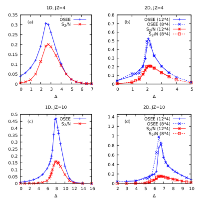
A quantity of interest is the Von Neumann entanglement entropy associated to the pure state . It can be computed for any bi-partition of the system, and is called the operator space entanglement entropy (OSEE) Prosen and Pižorn (2007). For a product state (), mixed or pure, the OSEE vanishes. For a pure state, the OSEE is twice the usual Von Neumann entropy associated to the same bipartition. This entropy quantifies the total amount of correlations, classical and/or quantum, between the two subsystems. It also quantifies how “demanding” it is to represent (or approximate) in an MPO form. Fig. 13 represents the steady state OSEE as a function of , for two values of at and . The partition considered here corresponds to a left-right cut in the center, with two subsystems of equal sizes. Both 1D chains and 2D cylinders are considered, and the results allow to identify the interesting range of where the steady state is the most correlated, and thus the most distant from a MF product state. In 2D cylinders the OSEE is expected to be proportional to the perimeter , which would be the analog of the “area-law” scaling for the entanglement entropy in pure states. Since the maximal value of the OSEE turns out here to be quite moderate (less than unity), it might be possible to investigate cylinders with a slightly larger perimeter in future studies.
The OSEE is sensitive to all (connected) correlations between the two subsystems, but it does not distinguish between classical and quantum correlations. In the case of pure states the Von Neumann entropy (of a subsystem) is the usual measure for entanglement, and it is specifically sensitive to quantum effects. But the entropy, computed from the reduced density matrix of a subsystem, is generically nonzero in any mixed state, even if the problem is purely classical. In the present model the steady-states are of course not completely classical, but in future studies it would be interesting to quantify the amount of “quantumness”, that is how far the state is from separable states.
VI Results beyond mean field
VI.1 Dimension one
As discussed in Landa et al. (2020) and shown also in Fig. 1, the difference between the steady state magnetization obtained in 1D with MPO and the MF ellipse increases with the interaction strength . This deviation is induced by the presence of nonzero correlations at distance in the lattice, as can be seen from (the exact) Eqs. (15)-(17). Figure 15 compares for MF, MFQF and MPO through the crossover region in , for a larger value of in 1D. The corrections to MF are significant for . To study the correlation functions we quantify the six independent components of by their discrete Fourier transform and the correlation length. Fig. 16 presents two lengthscales – the correlation length and the inverse of the dominant wavevector – which amounts to a dominant functional dependence on distance in the form
| (35) |
where , and are coefficients. In the heart of the crossover region across the MF bistability, the correlations calculated in MFQF or MPO in 1D chains grow by up to a few orders of magnitude, as measured by [see Eq. (33)]. As can be deduced from Fig. 16, the spatial structure of the two-point correlation functions undergoes a qualitative change within the crossover region. For low values the correlations have a relatively small amplitude, but they decay slowly with distance (large correlation length) and display some incommensurate density-wave character. On the other hand, for high , the correlations are very short-ranged (overdamped in space) and do not exhibit oscillations.
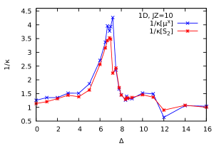
Although the system does not show any bistability, we observe some enhanced relaxation time in the crossover region, as shown in Fig. 14. There, the relaxation to the steady state was fitted to an exponential decay . The relaxation times associated to the -magnetization as well as that associated to the second Rényi entropy are shown. Although these two quantities are very different in nature, they give very similar relation times. The rate extracted from the dynamics of other observables, like or the OSEE for instance, also give very similar results. This suggests that we are here probing some intrinsic timescale of the model, proportional the inverse of the Liouvillian gap.
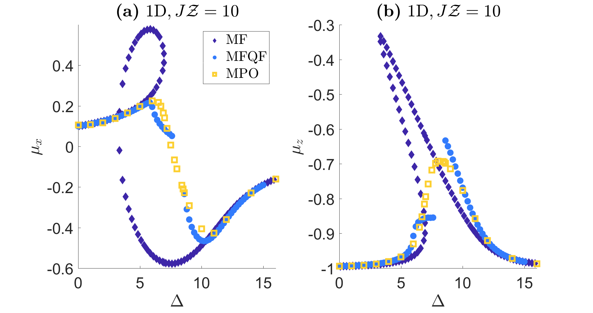
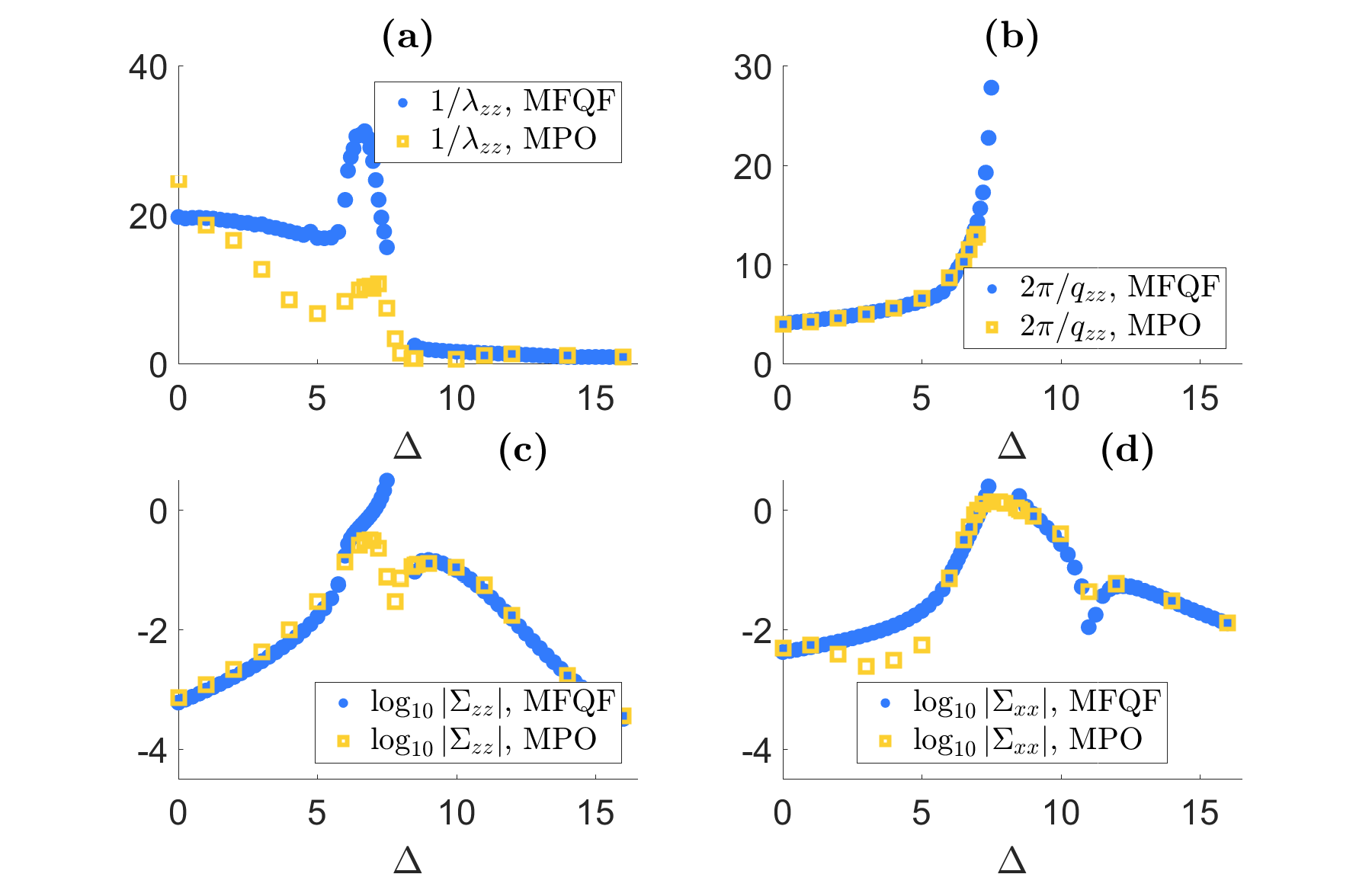
From Fig. 16 it can be seen that the crossover region is well captured by the MFQF approximation. Although quantitatively overestimated in the crossover region, the correlation length predicted by MFQF behaves in a way that is qualitatively very similar to that given my MPO calculations [Fig. 16(a)]. But what is quite remarkable is the agreement observed in Fig. 16(b) concerning the wave-vector of the modulations of the correlations. It appears that the MFQF formalism captures almost exactly this incommensurate character of the correlations. The magnitude of the correlations, probed here via and [see Eq. (33)], also behaves in a way that is qualitatively similar to the MPO data. We note, however, that for the MFQF approximation breaks down due to quantum fluctuations becoming too large and the correlators grow to nonphysical () values. For this reason, it is in this range that the deviations from the MPO results are the largest.
VI.2 Higher dimensions
As discussed in the introduction and in Landa et al. (2020), in dimension two and higher, MFQF predicts bistability. While in 2D our MPO simulations could be used to benchmark the MFQF results in regions where the correlation length is not too large, the accessible system size are relatively small, resulting necessarily in a unique steady state.
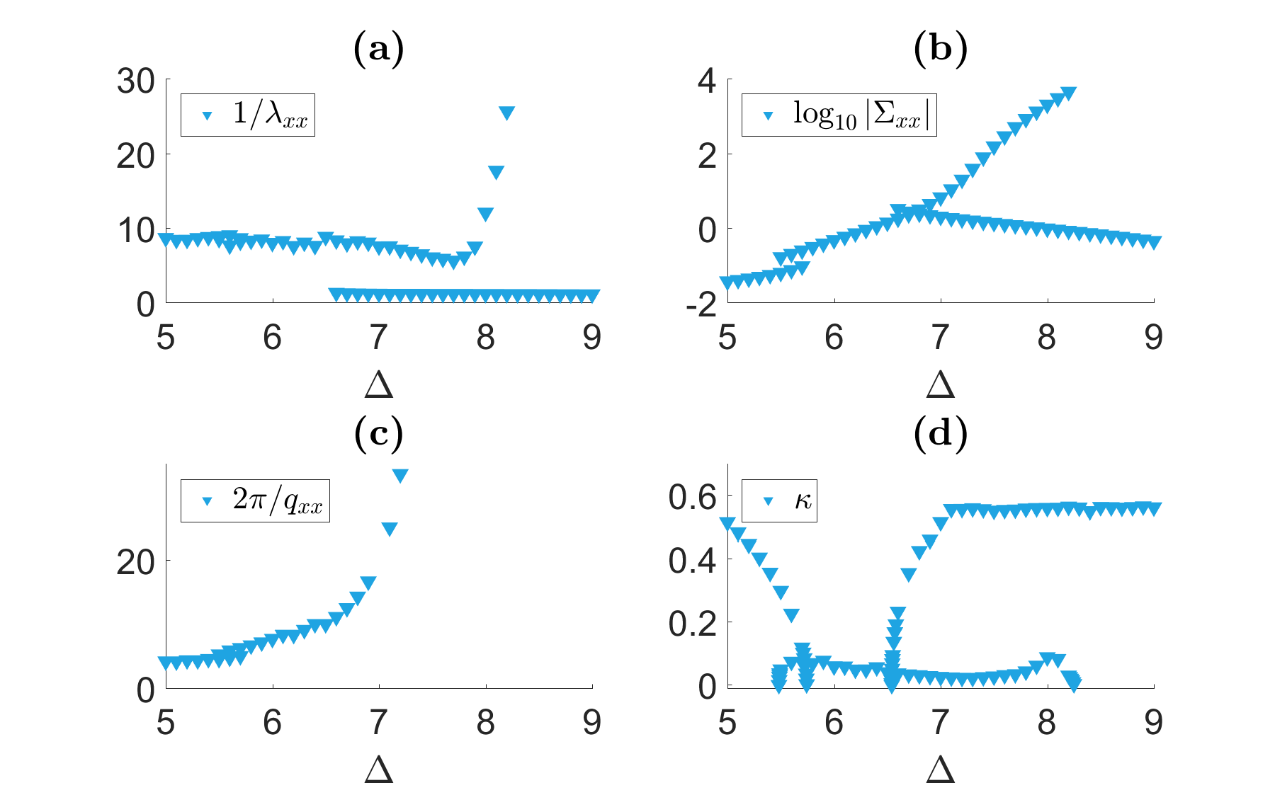
We therefore focus here on the MFQF results on 2D lattices, with the same parameters as the 1D example discussed above, with fixed (hence ). The MFQF approximation converges throughout the range presented in Fig. 2, and the maximal values taken by the correlation functions are smaller than in 1D. Figure 17 shows the characteristics of the correlation functions for the three steady-state branches. We find that the new emerging branch at intermediate magnetization values shares some properties with the MF-like branch that is stable at low values: a large correlation length and spatial oscillations characterized by . At the same time, the new branch has large absolute values of the correlation functions, as is the case with the MF-like branch that is stable at .
The inverse of the relaxation time to the steady state, , is plotted in Fig. 17(d). It is obtained by fitting , the time derivative of the square of the magnetization, to at large times (of order ). thus measures decay rate of small perturbations about the steady state. It can be seen that vanishes at the end points of each branch. In 2D we thus observe some critical slowing down at the edge of each branch (this holds in the MF approximation as well). Some important slowing down is also observed in the MPO calculations performed on cylinders, although the relaxation time cannot diverge on the small systems we considered.
As discussed briefly in Sec. II, we find that the new steady state and the limit cycle (LC) are stable in smaller regions as the dimension is increased. As with the LC, an exact characterization of this dependence is beyond the scope of the current work (and it becomes increasingly demanding to study the dependence of the results on as the dimension is increased).
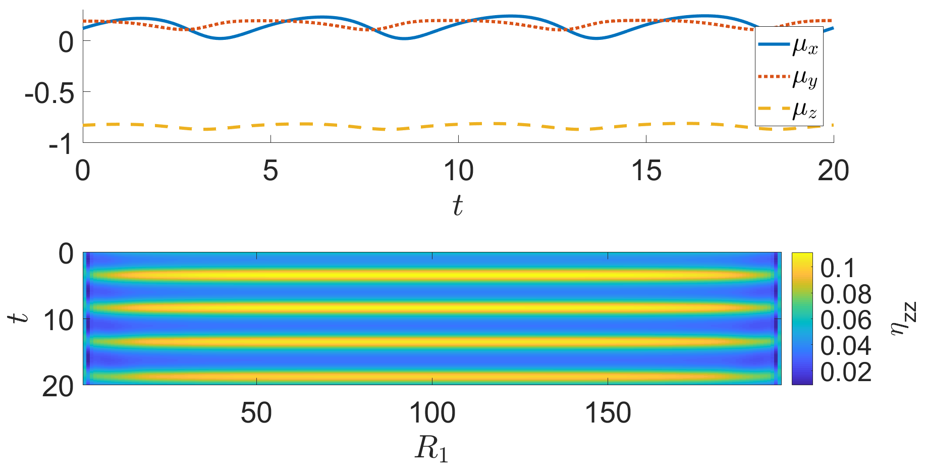
For (see Fig. 17), the correlation length in the new branch diverges, and beyond this point we find a stable LC, coexisting together with the MF-like branch in a small range (up to ). The amplitude of the magnetization oscillations varies with within the range of stability of the LC, and so does its frequency and other characteristics. In Fig. 18 we illustrate the LC phenomenon, showing oscillations of the mean magnetization as a function of time, and the space-time pattern in the correlation functions (along one spatial coordinate in the square lattice). In particular, the connected two-point function becomes spatially long-ranged at periodic intervals in time [yellow lines in Fig. 18].
VII Summary and Outlook
We have presented a detailed characterization of the MF limit of the driven-dissipative XY spin model, and studied some aspects of the associated dynamics such as the basins of attraction of different steady states. Going beyond MF, we have employed some accurate MPO-based method and the approximate MFQF approach. We have addressed the existence of multistability of the steady state predicted in MF, in addition to the possibility of states not captured by the MF limit, together with the spontaneous emergence of long-range spatial and temporal order.
As we have seen, in 1D the MFQF approach is capable of converging to a unique steady state, giving a picture which is very different from MF. As a comparison to MPO simulations shows, it is also capable to qualitatively and quantitatively predict some characteristics of the correlation functions, except in parameter regimes where the correlations become so large such that the neglect of three-point correlations (and higher) renders the approximation nonconverging. As the dimension is increased the correlations decrease in absolute magnitude. There, the MFQF is expected to become more accurate and this has been confirmed by comparison to MPO simulations of small 2D systems, for parameters that allow the comparison. It is straightforward to include in the MFQF formalism some more general local Lindblad terms acting on the spins, like the effect of dephasing. This could be a first immediate extension of the current work. Also, the investigation of other lattice geometries and/or longer-ranged spin interactions (as in Ates et al. (2012); Olmos et al. (2014); Parmee and Cooper (2019)), all of which are relevant for 2D systems of trapped ions, constitute interesting future directions.
The treatment of correlations in MFQF can account for two-point correlations with a large correlation length. This has allowed us to find a new steady state branch in 2D and higher, which is lacking in the MF limit. Clearly, the regimes with a large correlation length would be difficult to capture using methods based on small clusters. This intermediate branch shares some of its characteristics with the two MF-like steady states, making it suggestive to speculate that it may consist pictorially of coexisting domains. The correlation length in this branch diverges at some point, which may be an indication that the true quantum solution tends to develop long-range order in the form of a superposition. Beyond this critical point, MFQF predicts a correlation-induced limit cycle state, with correlation functions again extending over the simulated system size, and hence compatible with long-range spatio-temporal order. It should be noted that the MFQF approximation allows simulating very large lattices, but of course, it remains an open question how the inclusion of higher-order correlations would affect this behaviour.
The application of MPO simulations to 2D lattices, demonstrated here for the first time for a system with Lindblad dynamics, has proven successful. The numerical cost of such simulations is exponential in the perimeter () of the cylinder, but only linear in its length. This allows one to compute accurately in a controlled way not only the steady state properties, but also the transient dynamics of the system, for systems that are significantly larger than what is doable with an exact brute-force approach, while still keeping all the many-body correlations. In the present study we have been deliberately conservative, in the sense that we kept the systems sufficiently small so that the MPO calculations were essentially exact. These MPO calculations on small cylinders could then be used to benchmark the MFQF results in situations where the correlation length was small enough. It would of course be very interesting to push the 2D MPO simulations further in order to see if one can reach big enough systems and confirm the new phenomena predicted to occur in 2D by the MFQF approach.
Finally, we have shown that the basins of attraction of the new steady state progressively decrease with the dimension. We have also found that the parameter range of stability of the limit cycle again decreases with the dimension, possibly disappearing above 4D. Although it is hard to verify that these observations are independent of the simulated lattice sizes (due to the lateral lattice dimension accessible in our simulations necessarily decreasing with , while the correlation length much less, or not at all for some parameters), it provides a plausible explanation to the fact that these new phases do not survive in the MF limit. The possibility of simulating these spin models with controllable parameters using systems of trapped ions in 1D Brydges et al. (2019); Smith et al. (2016); Ramos and Cormick (2019) and 2D Bohnet et al. (2016), and arrays of superconducting qubits Houck et al. (2012); Schmidt and Koch (2013); Le Hur et al. (2016); Hartmann (2016); McKay et al. (2018); Alexander et al. (2020), holds a promise for exploring the emergence of phases with long spatial and temporal order out of the competition of coherent driving, dissipation, and strong interactions.
Acknowledgements.
We acknowledge the DRF of CEA for providing us with CPU time on the supercomputer COBALT of the CCRT. H.L. thanks Roni Geffen for fruitful discussions, and acknowledges support by IRS-IQUPS of Université Paris-Saclay and by LabEx PALM under grant number ANR-10-LABX-0039-PALM.Appendix A Further properties of the MF steady state
To understand the nature of the solutions as a function of all the parameters, we start by considering some simple limits. Using Eq. (28) we find that for ,
| (36) |
In the limit , the plane of Eq. (28) is nearly horizontal in the -space and , while for it is nearly vertical (see Fig. 7). In the latter case, combining Eq. (36) and the steady-state relation for ,
| (37) |
implies that for (with the other parameters fixed), and or (we have found that in all cases that we study, for the steady state is the infinite temperature state, ).
Fixing the value of the magnetization (within the constraints above), we can solve the steady state equations to obtain the model parameters and . If , we get and , and this requires . For we obtain
| (38) |
Hence, at fixed , is uniquely determined and we get a straight line in plane. Using Eq. (38) we find that the magnetization
| (39) |
occurs for along the line
| (40) |
The point is a critical point of the bistability region for . This is the only critical point at , as exemplified in Fig. 6. The magnetization is the unstable steady state solution along the line that crosses the bistable region.
Appendix B Equations of Motion
For spin one-half operators (Pauli matrices), we have the commutation relations, with ,
| (41) |
and the algebra of the ladder operators reads
| (42) |
For the local Hamiltonian terms we get
| (43) |
With the anti-commutation relations on the same site, , we get the known relation
| (44) |
that allows to simplify the dissipator terms when deriving the e.o.m.
The Hamiltonian part of the e.o.m for [Eq. (29)], can be derived most simply from the relation
| (45) |
and is obtained by multiplying Eqs. (III)-(10) by the required operator, and taking the expectation value. To derive the components of in Eq. (29) from Eqs. (III)-(10), we multiply the e.o.m of (with ) on the right by and expand the following series
| (46) |
By assuming for the three-point connected correlator of Eq. (14) [with ],
| (47) |
and using Eq. (44) we can simplify Eq. (46) to get
| (48) |
Multiplying on the left the e.o.m of by with ,
| (49) |
expanding we get
| (50) |
Let us derive of Eq. (29) separately for the two cases and (of course by linearity, they can be added). For , multiplying Eqs. (48)-(50) by with the correct sign and summing we get,
| (51) |
| (52) |
| (53) |
| (54) |
| (55) |
| (56) |
Appendix C Convergence of the MFQF method
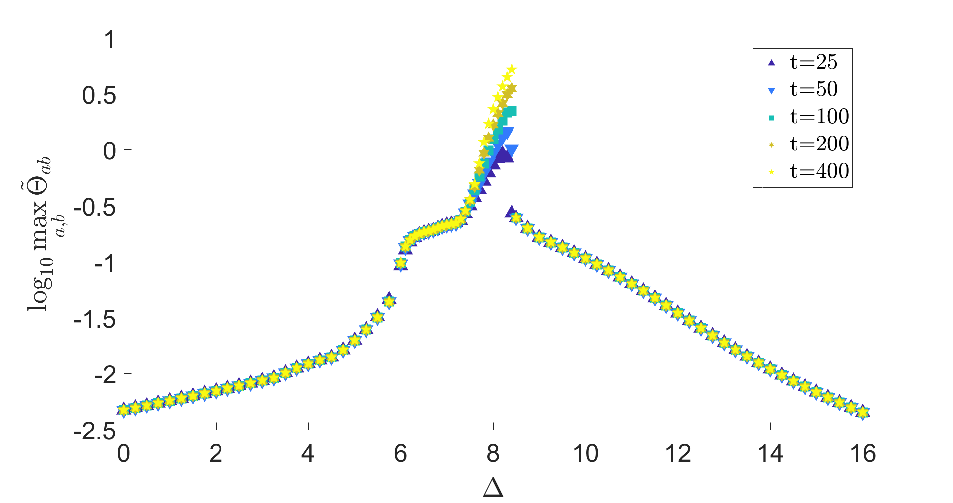
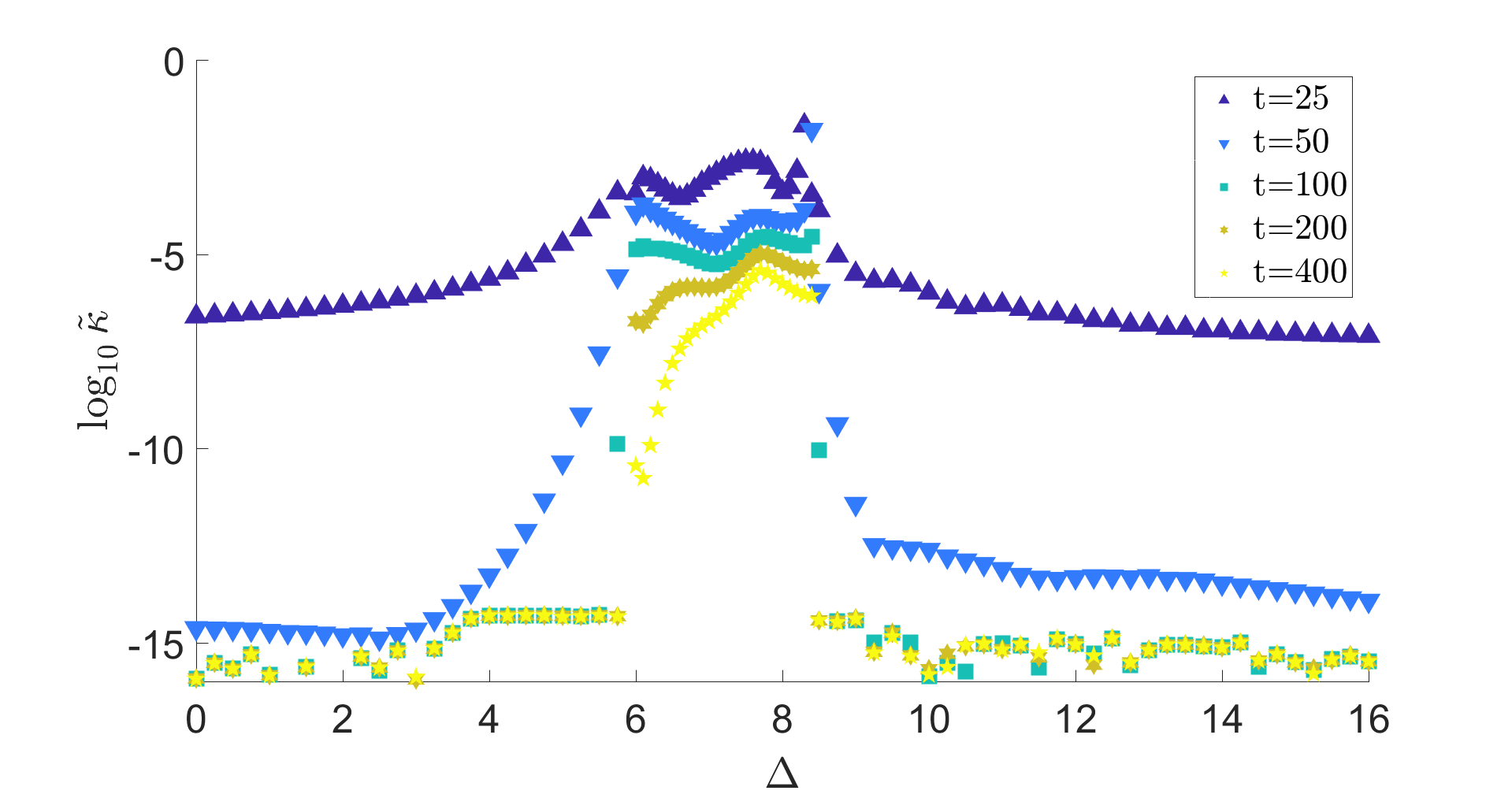
As a measure of the maximal correlations at a given time we take
| (65) |
where is a small averaging window. As a measure of the convergence of the dynamics we define using Eq. (64) in a similar interval,
| (66) |
We take and present results for and in a 1D chain in Figs. 19-20. In general, for and , we find that for there is a region (increasing in width with ) where the MFQF approximation breaks in 1D as the correlations become too large (a border that we define to be , a clearly unphysical value).
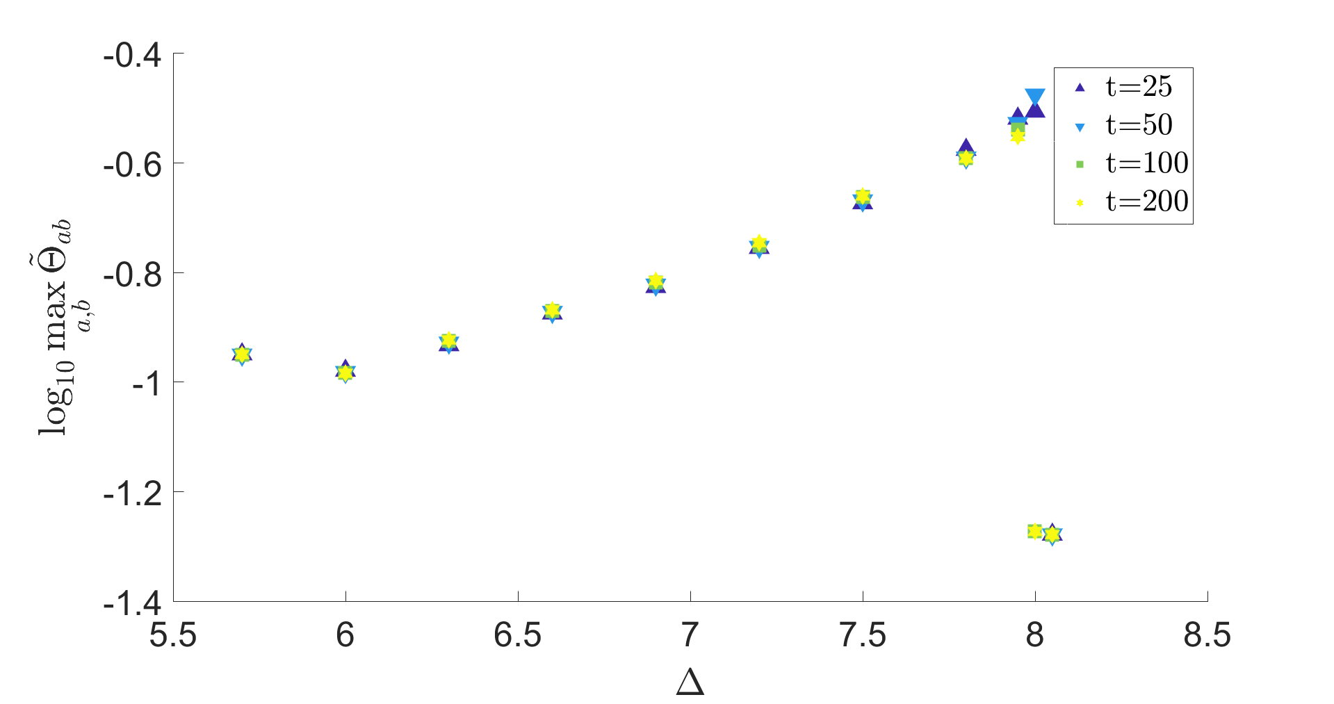
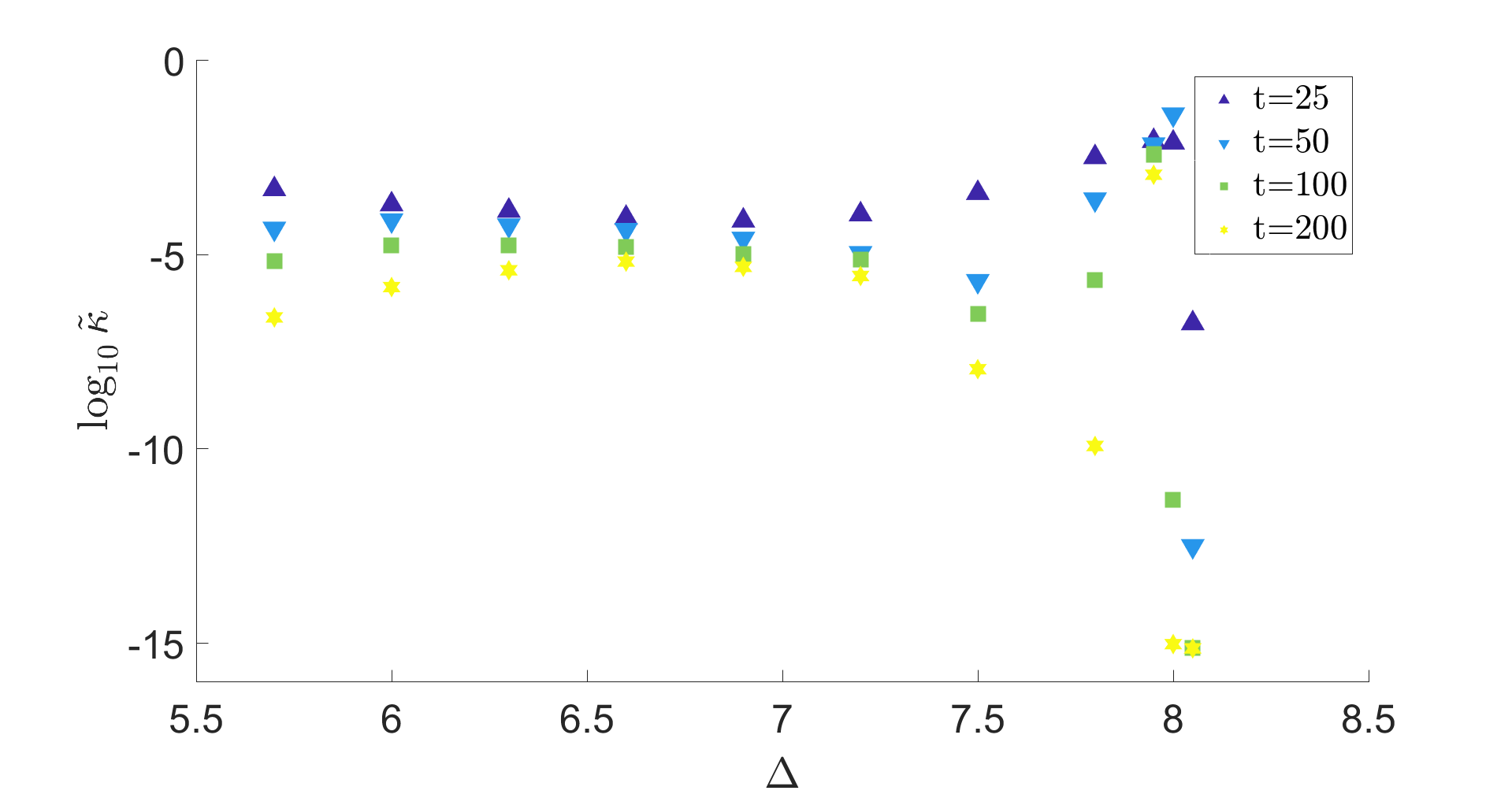
For 2D and higher dimensional lattices we did not find such cases, and the method has converged for the various parameter values that have been checked. In 2D we find that for the same parameters as in Fig. 19, with other components reaching . The correlation length shown in Fig. 17(a), which is at most 10-20 lattice sites up to the edge of the intermediate branch, implies that the simulations are well converged with the simulated lattice of sites. As the dimension is increased, decrease further, and also the typical correlation lengths for similar parameters decrease. In Figs. 21-22 we show the measure of convergence for a lattice in 3D (simulated with sites), for the intermediate branch and the same parameters, with the maximal correlation . We also find that the correlation length is at most 5-6 lattice sites for most values, until it starts to increase sharply, and in the range the correlation length assumes a magnitude of the order of the lateral lattice size available in the simulations.
Appendix D Convergence checks of the MPO calculations
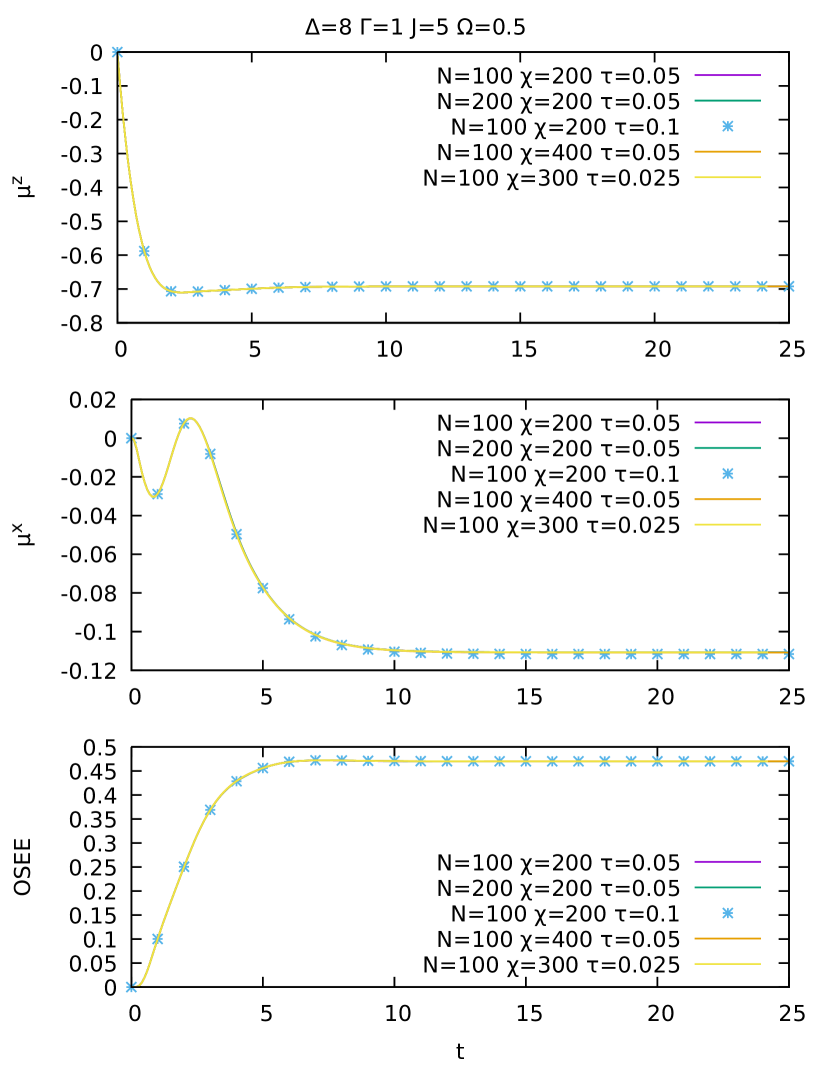
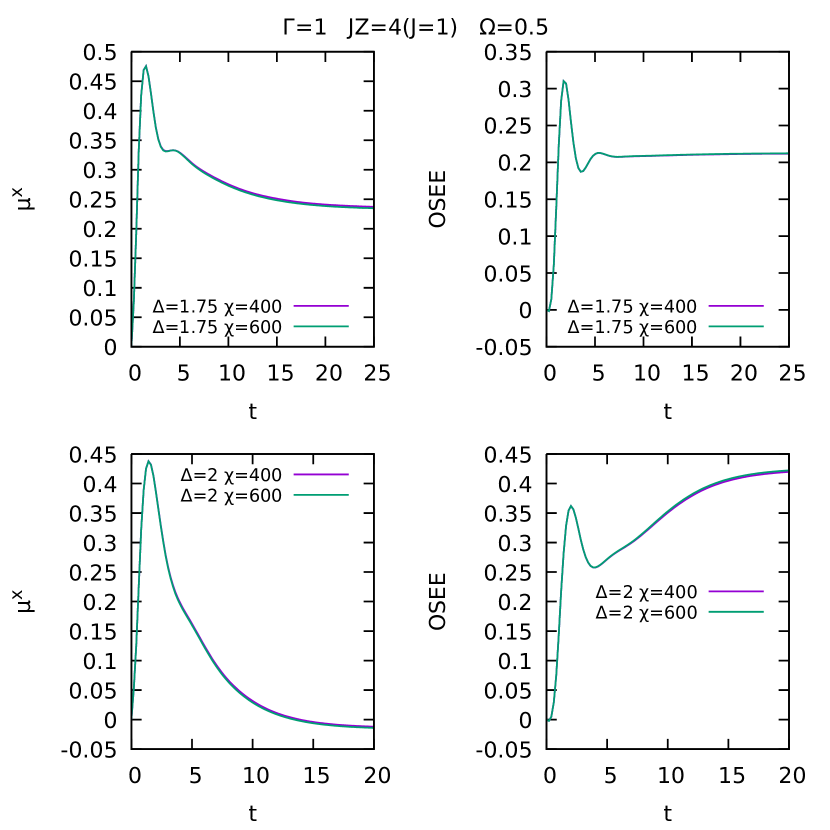
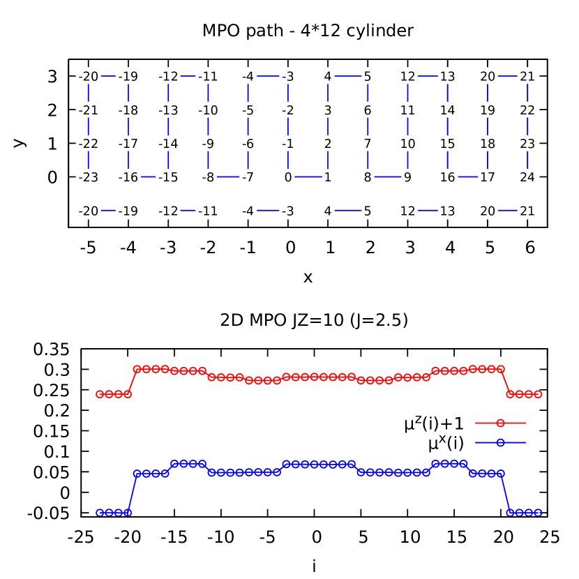
Our MPO implementation is based on the iTensor library ite (n 21), and encodes the Liouvillian super operator as a super-MPO (acting on the state which is an MPO). We evolve in real time using a Trotter scheme of order 4 Zaletel et al. (2015); Bidzhiev and Misguich (2017), with an error for each step which scale as . In the present study we typically used or (depending on the magnitude of the model parameters). Another crucial parameter is the maximum [bond] dimension used to truncate the Schmidt spectra after each singular value decomposition. The errors that are introduced can be estimated by checking how the relevant observables change when varying the parameters above. The results for 1D chains are summarized in Fig. 23. The effect of the finite bond dimension is illustrated in Fig. 24, where a simulation with is compared to one with .
Appendix E Transformation to the rotating frame
We consider a two-level system, represented by spin-1/2 operators. The energy difference between the two eigenstates (with eigenvalues 1 and -1) is modelled by the term
| (67) |
The driving term in the lab frame is a classical external field which couples to the spin, of amplitude and rotating at the angular frequency . It corresponds to the following term:
| (68) |
This could, for instance, describe the rotating electric field of a laser (or of a microwave) coupled to the two-level system Krantz et al. (2019). The mapping from this time-dependent Hamiltonian in the lab frame to a time-independent Hamiltonian (in the rotating frame) amounts to using the unitary transformation
| (69) |
and to considering the transformed density matrix . The Hamiltonian in the rotating frame is given by
| (70) |
which, making the rotating wave approximation (neglecting terms rotating with frequency , justified for ), results in the time-independent Hamiltonian
| (71) |
As for the jump terms, a simple calculation shows that they are not affected by the unitary transformation. This is because a unitary rotation of angle about the axis transforms into and into . Since a operator is always accompanied with a operator both in the coherent interaction terms and in the Lindblad dissipator terms, none are modified when going to the rotating frame.
References
- Houck et al. (2012) A. A. Houck, H. E. Türeci, and J. Koch, “On-chip quantum simulation with superconducting circuits,” Nature Physics 8, 292 (2012).
- Kubo et al. (2010) Y. Kubo, F. R. Ong, P. Bertet, D. Vion, V. Jacques, D. Zheng, A. Dréau, J.-F. Roch, A. Auffeves, F. Jelezko, J. Wrachtrup, M. F. Barthe, P. Bergonzo, and D. Esteve, “Strong Coupling of a Spin Ensemble to a Superconducting Resonator,” Phys. Rev. Lett. 105, 140502 (2010).
- Grezes et al. (2014) C. Grezes, B. Julsgaard, Y. Kubo, M. Stern, T. Umeda, J. Isoya, H. Sumiya, H. Abe, S. Onoda, T. Ohshima, V. Jacques, J. Esteve, D. Vion, D. Esteve, K. Mølmer, and P. Bertet, “Multimode Storage and Retrieval of Microwave Fields in a Spin Ensemble,” Phys. Rev. X 4, 021049 (2014).
- Fink et al. (2017) J. Fink, A. Dombi, A. Vukics, A. Wallraff, and P. Domokos, “Observation of the Photon-Blockade Breakdown Phase Transition,” Phys. Rev. X 7, 011012 (2017).
- Bruhat et al. (2016) L. Bruhat, J. Viennot, M. Dartiailh, M. Desjardins, T. Kontos, and A. Cottet, “Cavity Photons as a Probe for Charge Relaxation Resistance and Photon Emission in a Quantum Dot Coupled to Normal and Superconducting Continua,” Phys. Rev. X 6, 021014 (2016).
- Parlavecchio et al. (2015) O. Parlavecchio, C. Altimiras, J.-R. Souquet, P. Simon, I. Safi, P. Joyez, D. Vion, P. Roche, D. Esteve, and F. Portier, “Fluctuation-Dissipation Relations of a Tunnel Junction Driven by a Quantum Circuit,” Phys. Rev. Lett. 114, 126801 (2015).
- Bohnet et al. (2016) J. G. Bohnet, B. C. Sawyer, J. W. Britton, M. L. Wall, A. M. Rey, M. Foss-Feig, and J. J. Bollinger, “Quantum spin dynamics and entanglement generation with hundreds of trapped ions,” Science 352, 1297 (2016).
- Diehl et al. (2010) S. Diehl, A. Tomadin, A. Micheli, R. Fazio, and P. Zoller, “Dynamical Phase Transitions and Instabilities in Open Atomic Many-Body Systems,” Phys. Rev. Lett. 105, 015702 (2010).
- Keeling et al. (2010) J. Keeling, M. J. Bhaseen, and B. D. Simons, “Collective Dynamics of Bose-Einstein Condensates in Optical Cavities,” Phys. Rev. Lett. 105, 043001 (2010).
- Chang et al. (2008) D. E. Chang, V. Gritsev, G. Morigi, V. Vuletić, M. D. Lukin, and E. A. Demler, “Crystallization of strongly interacting photons in a nonlinear optical fibre,” Nature Physics 4, 884 (2008).
- Bhaseen et al. (2012) M. J. Bhaseen, J. Mayoh, B. D. Simons, and J. Keeling, “Dynamics of nonequilibrium Dicke models,” Phys. Rev. A 85, 013817 (2012).
- Otterbach et al. (2013) J. Otterbach, M. Moos, D. Muth, and M. Fleischhauer, “Wigner Crystallization of Single Photons in Cold Rydberg Ensembles,” Phys. Rev. Lett. 111, 113001 (2013).
- Höning et al. (2013) M. Höning, D. Muth, D. Petrosyan, and M. Fleischhauer, “Steady-state crystallization of Rydberg excitations in an optically driven lattice gas,” Phys. Rev. A 87, 023401 (2013).
- Carusotto and Ciuti (2013) I. Carusotto and C. Ciuti, “Quantum fluids of light,” Rev. Mod. Phys. 85, 299 (2013).
- Ritsch et al. (2013) H. Ritsch, P. Domokos, F. Brennecke, and T. Esslinger, “Cold atoms in cavity-generated dynamical optical potentials,” Rev. Mod. Phys. 85, 553 (2013).
- Schmidt and Koch (2013) S. Schmidt and J. Koch, “Circuit QED lattices: Towards quantum simulation with superconducting circuits,” Ann. Phys. (Berlin) 525, 395 (2013).
- Le Hur et al. (2016) K. Le Hur, L. Henriet, A. Petrescu, K. Plekhanov, G. Roux, and M. Schiró, “Many-body quantum electrodynamics networks: Non-equilibrium condensed matter physics with light,” Comptes Rendus Physique 17, 808 (2016).
- Noh and Angelakis (2017) C. Noh and D. G. Angelakis, “Quantum simulations and many-body physics with light,” Rep. Prog. Phys. 80, 016401 (2017).
- Hartmann (2016) M. J. Hartmann, “Quantum simulation with interacting photons,” J. Opt. 18, 104005 (2016).
- Schiró et al. (2016) M. Schiró, C. Joshi, M. Bordyuh, R. Fazio, J. Keeling, and H. Türeci, “Exotic Attractors of the Nonequilibrium Rabi-Hubbard Model,” Phys. Rev. Lett. 116, 143603 (2016).
- Greentree et al. (2006) A. D. Greentree, C. Tahan, J. H. Cole, and L. C. L. Hollenberg, “Quantum phase transitions of light,” Nature Physics 2, 856 (2006).
- Hartmann et al. (2006) M. J. Hartmann, F. G. S. L. Brandão, and M. B. Plenio, “Strongly interacting polaritons in coupled arrays of cavities,” Nature Physics 2, 849 (2006).
- Nagy et al. (2011) D. Nagy, G. Szirmai, and P. Domokos, “Critical exponent of a quantum-noise-driven phase transition: The open-system Dicke model,” Phys. Rev. A 84, 043637 (2011).
- Öztop et al. (2012) B. Öztop, M. Bordyuh, O. E. Müstecaplıoğlu, and H. E. Türeci, “Excitations of optically driven atomic condensate in a cavity: theory of photodetection measurements,” New J. Phys. 14, 085011 (2012).
- Schiró et al. (2012) M. Schiró, M. Bordyuh, B. Öztop, and H. E. Türeci, “Phase Transition of Light in Cavity QED Lattices,” Phys. Rev. Lett. 109, 053601 (2012).
- Schiró et al. (2013) M. Schiró, M. Bordyuh, B. Öztop, and H. E. Türeci, “Quantum phase transition of light in the Rabi–Hubbard model,” J. Phys. B: At. Mol. Opt. Phys. 46, 224021 (2013).
- Torre et al. (2013) E. G. D. Torre, S. Diehl, M. D. Lukin, S. Sachdev, and P. Strack, “Keldysh approach for nonequilibrium phase transitions in quantum optics: Beyond the Dicke model in optical cavities,” Phys. Rev. A 87, 023831 (2013).
- Kulkarni et al. (2013) M. Kulkarni, B. Öztop, and H. E. Türeci, “Cavity-Mediated Near-Critical Dissipative Dynamics of a Driven Condensate,” Phys. Rev. Lett. 111, 220408 (2013).
- Brennecke et al. (2013) F. Brennecke, R. Mottl, K. Baumann, R. Landig, T. Donner, and T. Esslinger, “Real-time observation of fluctuations at the driven-dissipative Dicke phase transition,” PNAS 110, 11763 (2013).
- Fitzpatrick et al. (2017) M. Fitzpatrick, N. M. Sundaresan, A. C. Li, J. Koch, and A. A. Houck, “Observation of a Dissipative Phase Transition in a One-Dimensional Circuit QED Lattice,” Phys. Rev. X 7, 011016 (2017).
- Scarlatella et al. (2019) O. Scarlatella, R. Fazio, and M. Schiró, “Emergent finite frequency criticality of driven-dissipative correlated lattice bosons,” Phys. Rev. B 99, 064511 (2019).
- Ma et al. (2019) R. Ma, B. Saxberg, C. Owens, N. Leung, Y. Lu, J. Simon, and D. I. Schuster, “A dissipatively stabilized mott insulator of photons,” Nature 566, 51 (2019).
- Marino and Diehl (2016) J. Marino and S. Diehl, “Quantum dynamical field theory for nonequilibrium phase transitions in driven open systems,” Phys. Rev. B 94, 085150 (2016).
- Shchadilova et al. (2020) Y. Shchadilova, M. M. Roses, E. G. Dalla Torre, M. D. Lukin, and E. Demler, “Fermionic formalism for driven-dissipative multilevel systems,” Phys. Rev. A 101, 013817 (2020).
- Kirton et al. (2019) P. Kirton, M. M. Roses, J. Keeling, and E. G. Dalla Torre, “Introduction to the dicke model: From equilibrium to nonequilibrium, and vice versa,” Advanced Quantum Technologies 2, 1800043 (2019), https://onlinelibrary.wiley.com/doi/pdf/10.1002/qute.201800043 .
- Sánchez Muñoz et al. (2019) C. Sánchez Muñoz, B. Buča, J. Tindall, A. González-Tudela, D. Jaksch, and D. Porras, “Symmetries and conservation laws in quantum trajectories: Dissipative freezing,” Phys. Rev. A 100, 042113 (2019).
- Munoz et al. (2019) C. S. Munoz, B. Buča, J. Tindall, A. González-Tudela, D. Jaksch, and D. Porras, “Spontaneous freezing in driven-dissipative quantum systems,” arXiv preprint arXiv:1903.05080 (2019).
- Bardyn et al. (2013) C.-E. Bardyn, M. A. Baranov, C. V. Kraus, E. Rico, A. Imamoğlu, P. Zoller, and S. Diehl, “Topology by dissipation,” New J. Phys. 15, 085001 (2013).
- Oka and Kitamura (2019) T. Oka and S. Kitamura, “Floquet Engineering of Quantum Materials,” Annual Review of Condensed Matter Physics 10, 387 (2019).
- Koch et al. (2010) J. Koch, A. A. Houck, K. L. Hur, and S. M. Girvin, “Time-reversal-symmetry breaking in circuit-QED-based photon lattices,” Phys. Rev. A 82, 043811 (2010).
- Petrescu et al. (2012) A. Petrescu, A. A. Houck, and K. Le Hur, “Anomalous Hall effects of light and chiral edge modes on the kagomé lattice,” Phys. Rev. A 86, 053804 (2012).
- Hafezi et al. (2013a) M. Hafezi, S. Mittal, J. Fan, A. Migdall, and J. M. Taylor, “Imaging topological edge states in silicon photonics,” Nature Photonics 7, 1001 (2013a).
- Cho et al. (2008) J. Cho, D. G. Angelakis, and S. Bose, “Fractional Quantum Hall State in Coupled Cavities,” Phys. Rev. Lett. 101, 246809 (2008).
- Umucalılar and Carusotto (2011) R. O. Umucalılar and I. Carusotto, “Artificial gauge field for photons in coupled cavity arrays,” Phys. Rev. A 84, 043804 (2011).
- Hafezi et al. (2013b) M. Hafezi, M. D. Lukin, and J. M. Taylor, “Non-equilibrium fractional quantum Hall state of light,” New J. Phys. 15, 063001 (2013b).
- Rechtsman et al. (2013) M. C. Rechtsman, J. M. Zeuner, Y. Plotnik, Y. Lumer, D. Podolsky, F. Dreisow, S. Nolte, M. Segev, and A. Szameit, “Photonic Floquet topological insulators,” Nature 496, 196 (2013).
- Lee et al. (2011) T. E. Lee, H. Häffner, and M. C. Cross, “Antiferromagnetic phase transition in a nonequilibrium lattice of Rydberg atoms,” Phys. Rev. A 84, 031402 (2011).
- Qian et al. (2012) J. Qian, G. Dong, L. Zhou, and W. Zhang, “Phase diagram of Rydberg atoms in a nonequilibrium optical lattice,” Phys. Rev. A 85, 065401 (2012).
- Jin et al. (2013) J. Jin, D. Rossini, R. Fazio, M. Leib, and M. J. Hartmann, “Photon Solid Phases in Driven Arrays of Nonlinearly Coupled Cavities,” Phys. Rev. Lett. 110, 163605 (2013).
- Jin et al. (2014) J. Jin, D. Rossini, M. Leib, M. J. Hartmann, and R. Fazio, “Steady-state phase diagram of a driven QED-cavity array with cross-Kerr nonlinearities,” Phys. Rev. A 90, 023827 (2014).
- Parmee and Cooper (2018) C. D. Parmee and N. R. Cooper, “Phases of driven two-level systems with nonlocal dissipation,” Phys. Rev. A 97, 053616 (2018).
- Foss-Feig et al. (2017) M. Foss-Feig, P. Niroula, J. T. Young, M. Hafezi, A. V. Gorshkov, R. M. Wilson, and M. F. Maghrebi, “Emergent equilibrium in many-body optical bistability,” Phys. Rev. A 95, 043826 (2017).
- Biondi et al. (2017a) M. Biondi, G. Blatter, H. E. Türeci, and S. Schmidt, “Nonequilibrium gas-liquid transition in the driven-dissipative photonic lattice,” Phys. Rev. A 96, 043809 (2017a).
- Chan et al. (2015) C.-K. Chan, T. E. Lee, and S. Gopalakrishnan, “Limit-cycle phase in driven-dissipative spin systems,” Phys. Rev. A 91, 051601 (2015).
- Wilson et al. (2016) R. M. Wilson, K. W. Mahmud, A. Hu, A. V. Gorshkov, M. Hafezi, and M. Foss-Feig, “Collective phases of strongly interacting cavity photons,” Phys. Rev. A 94, 033801 (2016).
- Marcuzzi et al. (2014) M. Marcuzzi, E. Levi, S. Diehl, J. P. Garrahan, and I. Lesanovsky, “Universal Nonequilibrium Properties of Dissipative Rydberg Gases,” Phys. Rev. Lett. 113, 210401 (2014).
- Iemini et al. (2018) F. Iemini, A. Russomanno, J. Keeling, M. Schirò, M. Dalmonte, and R. Fazio, “Boundary time crystals,” Phys. Rev. Lett. 121, 035301 (2018).
- Biondi et al. (2017b) M. Biondi, S. Lienhard, G. Blatter, H. E. Türeci, and S. Schmidt, “Spatial correlations in driven-dissipative photonic lattices,” New J. Phys. 19, 125016 (2017b).
- Biondi et al. (2018) M. Biondi, S. Lienhard, G. Blatter, and S. Schmidt, “Quantum stabilization of photonic spatial correlations,” Phys. Scr. 94, 024001 (2018).
- Weimer (2015) H. Weimer, “Variational Principle for Steady States of Dissipative Quantum Many-Body Systems,” Phys. Rev. Lett. 114, 040402 (2015).
- Mendoza-Arenas et al. (2016) J. J. Mendoza-Arenas, S. R. Clark, S. Felicetti, G. Romero, E. Solano, D. G. Angelakis, and D. Jaksch, “Beyond mean-field bistability in driven-dissipative lattices: Bunching-antibunching transition and quantum simulation,” Phys. Rev. A 93, 023821 (2016).
- Vicentini et al. (2018) F. Vicentini, F. Minganti, R. Rota, G. Orso, and C. Ciuti, “Critical slowing down in driven-dissipative Bose-Hubbard lattices,” Phys. Rev. A 97, 013853 (2018).
- Landa et al. (2020) H. Landa, M. Schiró, and G. Misguich, “Multistability of driven-dissipative quantum spins,” Physical Review Letters 124, 043601 (2020).
- Jin et al. (2018) J. Jin, A. Biella, O. Viyuela, C. Ciuti, R. Fazio, and D. Rossini, “Phase diagram of the dissipative quantum Ising model on a square lattice,” Phys. Rev. B 98, 241108 (2018).
- Kshetrimayum et al. (2017) A. Kshetrimayum, H. Weimer, and R. Orús, “A simple tensor network algorithm for two-dimensional steady states,” Nature Communications 8, 1291 (2017).
- Minganti et al. (2018) F. Minganti, A. Biella, N. Bartolo, and C. Ciuti, “Spectral theory of liouvillians for dissipative phase transitions,” Phys. Rev. A 98, 042118 (2018).
- Owen et al. (2018) E. T. Owen, J. Jin, D. Rossini, R. Fazio, and M. J. Hartmann, “Quantum correlations and limit cycles in the driven-dissipative Heisenberg lattice,” New J. Phys. 20, 045004 (2018).
- Sandri et al. (2012) M. Sandri, M. Schiró, and M. Fabrizio, “Linear ramps of interaction in the fermionic Hubbard model,” Phys. Rev. B 86, 075122 (2012).
- Zwolak and Vidal (2004) M. Zwolak and G. Vidal, “Mixed-State Dynamics in One-Dimensional Quantum Lattice Systems: A Time-Dependent Superoperator Renormalization Algorithm,” Phys. Rev. Lett. 93, 207205 (2004).
- Verstraete et al. (2004) F. Verstraete, J. J. García-Ripoll, and J. I. Cirac, “Matrix Product Density Operators: Simulation of Finite-Temperature and Dissipative Systems,” Phys. Rev. Lett. 93, 207204 (2004).
- Prosen and Žnidarič (2009) T. Prosen and M. Žnidarič, “Matrix product simulations of non-equilibrium steady states of quantum spin chains,” J. Stat. Mech. 2009, P02035 (2009).
- Benenti et al. (2009) G. Benenti, G. Casati, T. Prosen, D. Rossini, and M. Žnidarič, “Charge and spin transport in strongly correlated one-dimensional quantum systems driven far from equilibrium,” Phys. Rev. B 80, 035110 (2009).
- Mascarenhas et al. (2015) E. Mascarenhas, H. Flayac, and V. Savona, “Matrix-product-operator approach to the nonequilibrium steady state of driven-dissipative quantum arrays,” Phys. Rev. A 92, 022116 (2015).
- Stoudenmire and White (2012) E. Stoudenmire and S. R. White, “Studying Two-Dimensional Systems with the Density Matrix Renormalization Group,” Annu. Rev. Condens. Matter Phys. 3, 111 (2012).
- Prosen and Pižorn (2007) T. Prosen and I. Pižorn, “Operator space entanglement entropy in a transverse Ising chain,” Phys. Rev. A 76, 032316 (2007).
- Ates et al. (2012) C. Ates, B. Olmos, J. P. Garrahan, and I. Lesanovsky, “Dynamical phases and intermittency of the dissipative quantum Ising model,” Phys. Rev. A 85, 043620 (2012).
- Olmos et al. (2014) B. Olmos, D. Yu, and I. Lesanovsky, “Steady-state properties of a driven atomic ensemble with nonlocal dissipation,” Phys. Rev. A 89, 023616 (2014).
- Parmee and Cooper (2019) C. D. Parmee and N. R. Cooper, “Steady states of a driven dissipative dipolar XXZ chain,” arXiv:1906.10953 (2019).
- Brydges et al. (2019) T. Brydges, A. Elben, P. Jurcevic, B. Vermersch, C. Maier, B. P. Lanyon, P. Zoller, R. Blatt, and C. F. Roos, “Probing Rényi entanglement entropy via randomized measurements,” Science 364, 260 (2019).
- Smith et al. (2016) J. Smith, A. Lee, P. Richerme, B. Neyenhuis, P. W. Hess, P. Hauke, M. Heyl, D. A. Huse, and C. Monroe, “Many-body localization in a quantum simulator with programmable random disorder,” Nature Physics 12, 907 (2016).
- Ramos and Cormick (2019) A. Ramos and C. Cormick, “Feasibility of the ion-trap simulation of a class of non-equilibrium phase transitions,” The European Physical Journal D 73, 237 (2019).
- McKay et al. (2018) D. C. McKay, T. Alexander, L. Bello, M. J. Biercuk, L. Bishop, J. Chen, J. M. Chow, A. D. Córcoles, D. Egger, S. Filipp, et al., “Qiskit backend specifications for openqasm and openpulse experiments,” arXiv preprint arXiv:1809.03452 (2018).
- Alexander et al. (2020) T. Alexander, N. Kanazawa, D. J. Egger, L. Capelluto, C. J. Wood, A. Javadi-Abhari, and D. McKay, “Qiskit pulse: Programming quantum computers through the cloud with pulses,” arXiv preprint arXiv:2004.06755 (2020).
- ite (n 21) ITensor Library, http://itensor.org (version 2.1).
- Zaletel et al. (2015) M. P. Zaletel, R. S. K. Mong, C. Karrasch, J. E. Moore, and F. Pollmann, “Time-evolving a matrix product state with long-ranged interactions,” Phys. Rev. B 91, 165112 (2015).
- Bidzhiev and Misguich (2017) K. Bidzhiev and G. Misguich, “Out-of-equilibrium dynamics in a quantum impurity model: Numerics for particle transport and entanglement entropy,” Phys. Rev. B 96, 195117 (2017).
- Krantz et al. (2019) P. Krantz, M. Kjaergaard, F. Yan, T. P. Orlando, S. Gustavsson, and W. D. Oliver, “A quantum engineer’s guide to superconducting qubits,” Applied Physics Reviews 6, 021318 (2019).