Theory of magnetic response in finite two-dimensional superconductors

Abstract

We present a theory of magnetic response in a finite-size two-dimensional superconductors with Rashba spin-orbit coupling. The interplay between the latter and an in-plane Zeeman field leads on the one hand to an out-of-plane spin polarization which accumulates at the edges of the sample over the superconducting coherence length, and on the other hand, to circulating supercurrents decaying away from the edge over a macroscopic scale. In a long finite stripe of width $W$ both, the spin polarization and the currents, contribute to the total magnetic moment induced at the stripe ends. These two contributions scale with powers of $W$ such that for sufficiently large samples it can be detected by current magnetometry techniques.

Superconductivity in two-dimensional (2D) and quasi-2D systems has been attracting a great deal of attention over past decades Uchihashi (2016); Saito et al. (2017). Examples of such systems range from ultra-thin metallic films, heavy fermion superlattices, and interfacial superconductors to atomic layers of metal dichalcogenides, and organic conductors.

Most 2D superconductors exhibit large spin-orbit coupling (SOC) because of broken space inversion symmetry. In this regard two types of 2D superconductors can be distinguished: Those exhibiting SOC of Rashba-type due to a broken up-down (out-of-plane) mirror symmetry, denoted here as Rashba superconductors, and those, in which a 2D in-plane inversion symmetry is broken due to a non-centrosymmetric crystal structure. The latter are exemplified by 2D transition metal dichalcogenides Saito et al. (2016); Lu et al. (2015). To the first group, on which we focus here, belong for example ultra-thin superconducting metallic films Gruznev et al. (2014); Sekihara et al. (2013); Ménard et al. (2017).

Over the last years Rashba superconductors have been intensively studied as paradigmatic systems where pair correlations coexist with strong intrinsic SOC Edelstein (1989, 1995, 1996); Yip (2002); Gor’kov and Rashba (2001); Frigeri et al. (2004); Edelstein (2008); Agterberg and Kaur (2007); Dimitrova and Feigelman (2003); Dimitrova and Feigel?Man (2007); Pershoguba et al. (2015); Mal’shukov (2016); Konschelle et al. (2015). Because of the interplay between SOC and a Zeeman field they demonstrate highly unusual properties, such as, the appearance of an inhomogeneous superconducting phase Dimitrova and Feigel?Man (2007); Agterberg and Kaur (2007), magnetoelectric effects Edelstein (1995); Yip (2002); Konschelle et al. (2015), and anisotropic magnetic susceptibility Gor’kov and Rashba (2001). With few exceptions, as for example Refs. Edelstein (2003); Pershoguba et al. (2015); Mal’shukov (2016), most of these works focused on infinite 2D systems.

In this letter we demonstrate that finite size effects drastically modify the magnetic response of Rashba superconductors leading to hitherto unknown phenomena. Our main findings are the following: (i) In a response to a Zeeman field the system exhibits a spin texture (Fig. 1a) with a transverse component of the spin localized near the edge on the scale of superconducting coherence length. (ii) Because of the spin-charge coupling mediated by the SOC, a non-homogenous charge current appears in the system with a spatial distribution that depends on the direction of the applied field and geometry of the system (Fig. 1b); (iii) In particular, for a finite stripe oriented along the field, macroscopic currents loops appear at the stripe ends (Fig. 1c). Both, the transverse spin and the edge currents contribute to the total magnetic moment which can be detected by state-of-the-art magnetometry techniques.

These findings can be qualitatively understood recalling the concepts of spin currents and spin galvanic effect (see Fig. 1). The key feature of 2D materials without up-down mirror symmetry is the Rashba SOC, $H_{R}=\alpha({\bf e}_{z}\times{\bf v})\cdot{\bm{\sigma}}$. Here ${\bf e}_{z}$ is a vector normal to the 2D plane, ${\bf v}={\bf p}/2m$ is the quasiparticle velocity, $m$ its effective mass, ${\bm{\sigma}}$ is the vector of Pauli matrices, and $\alpha$ is the SOC constant . The SOC acts as an effective ${\bf p}$-dependent spin splitting field. Let us assume that the system is subject to an external Zeeman field ${\bf B}$, and for some reason the induced spin polarization ${\bf S}$ differs from the equilibrium Pauli response $\chi_{P}{\bf B}$, where $\chi_{P}$ is the Pauli paramagnetic polarizability. Then the excess spin $\delta{\bf S}={\bf S}-\chi_{P}{\bf B}$ will experience an inhomogeneous precession in the effective Rashba field, generating a momentum anisotropy of the density matrix. In the presence of disorder the precession rate $\hat{R}=i[H_{R},\delta{\bf S}\cdot\bm{\sigma}]$ is balanced by the momentum relaxation, which results in a steady spin current in the bulk of the system ${\cal J}_{bulk,k}^{a}=-\tau{\rm tr}\langle v_{k}\sigma^{a}\hat{R}\rangle=\alpha D(\delta S^{z}\delta_{ka}-\delta S^{k}\delta_{az})$, where $\tau$ is the momentum relaxation time, and $D=\tau v_{F}^{2}/{2}$ is the diffusion coefficient. Under equilibrium conditions $\delta{\bf S}=0$ in normal systems, but in superconductors pair correlations modify the Pauli response leading to a finite $\delta{\bf S}$ Abrikosov and Gor’kov (1962); Gor’kov and Rashba (2001). This leads to finite equilibrium spin-currents in Rashba superconductors generated by the Zeeman field. For example, a field applied in $x$-direction in a bulk superconductor produces a spin-current with an out-of-plane polarization, ${\cal J}_{bulk,x}^{z}=-\alpha D\delta S^{x}$. Due to the spin-Hall magneto-electric coupling in Rashba materials the bulk spin-current generates a transverse charge current according to $j_{bulk,y}\propto\alpha^{2}{\cal J}_{bulk,x}^{z}=\alpha^{3}D\delta S^{x}$, which is nothing, but the anomalous supercurrent well known for bulk superconductors with SOC Edelstein (1989); Yip (2002); Dimitrova and Feigel?Man (2007).

In a finite system currents must vanish at the edges of the sample. This condition can be fulfilled only if the distribution of the excess spin $\delta{\bf S}({\bf r})$ is inhomogeneous near the edge, so that the diffusion spin-current ${\cal J}_{diff,k}^{a}=-D\partial_{k}\delta S^{a}$ compensates the bulk contribution. For concreteness, if we assume a boundary with vacuum at $x=0$, the zero spin-current condition for a field applied in $x$-direction reads: $D\partial_{x}\delta S^{z}={\cal J}_{bulk,x}^{z}$, which implies that a finite component $\delta S^{z}(x)$ transverse to the field is induced at the edges of the sample. In this case the spin density exhibits a texture as sketched in Fig. 1a tokatly2019correspondence . In the presence of SOC both the edge and the bulk spin-currents are converted into a charge current flowing parallel to the boundary, via the spin-galvanic effect, Fig. 1b. In a realistic finite system currents must vanish at all edges. The anomalous charge currents at the boundaries should then be compensated by supercurrents which stem from a gradient of the superconducting phase. As a consequence, in a stripe geometry, an in-plane field induces current loops at the edges as shown in Fig. 1c. The magnetic moment induced by this currents and by the transverse spin can in principle be measured to directly detect the effects we predict here. In the rest of the paper we provide a quantitative derivation of these effects, calculate the induced magnetic moment, and propose materials in which our predictions can be verified.

Specifically, we consider a 2D disordered superconductor with Rashba SOC. We assume that the Fermi energy corresponds to the largest energy scale, so that spectral and transport properties can be accurately described by the quasiclassical Green’s functions (GFs) Eilenberger (1968); Larkin and Ovchinnikov (1969). In the diffusive limit these functions are isotropic in momentum and they obey the Usadel equation which in the presence of a Zeeman field and Rashba SOC reads Bergeret et al. (2005); Bergeret and Tokatly (2013, 2014):

$$D\tilde{\nabla}_{k}\left(\check{g}\tilde{\nabla}_{k}\check{g}\right)-\left[\left(\omega+i{\bf h}\cdot\bm{\sigma}\right)\tau_{3}+\Delta\tau_{2},\check{g}\right]=0\quad.$$ (1)

Here ${\bf h}=\mu_{B}{\bf B}$, ${\bm{\sigma}}=(\sigma^{x},\sigma^{y},\sigma^{z})$ and $\tau_{2,3}$ are Pauli matrices spanning spin and Nambu space, respectively, $\omega$ is the Matsubara frequency, $\Delta$ is the superconducting order parameter, and SOC enters via the covariant derivative $\tilde{\nabla}_{k}\check{g}=\partial_{k}\check{g}-i\left[\hat{{\cal A}}_{k},\check{g}\right]$, where $\hat{{\cal A}}_{k}=\alpha\left(\delta_{kx}\sigma^{y}-\delta_{ky}\sigma^{x}\right)$, summation over repeated indices is implied, and $k=x,y$ . The quasiclassical GF $\check{g}$ in Eq. (1) is a 4$\times$4 matrix in the Nambu-spin space, which satisfies the normalization condition $\check{g}^{2}=1$. In the absence of spin-dependent fields it reads $\check{g}_{0}=(\omega/E)\tau_{3}+(\Delta/E)\tau_{2}$, where $E=\sqrt{\omega^{2}+\Delta^{2}}$. It is easy to check by substitution into Eq. (1), that in the absence of Zeeman field $\check{g}_{0}$ is also the solution of the Usadel equation for arbitrary $\hat{{\cal A}}_{k}$.

To compute the response to an external magnetic field we linearize Eq. (1) with respect to $\bf h$ and write the solution as $\check{g}\approx\check{g}_{0}+\delta\check{g}$. It is convenient to define $\delta\check{g}\equiv i\check{g}_{0}\left[\tau_{3},\check{g}_{0}\right]\hat{Q}$, where $\hat{Q}$ is a matrix in spin space that satisfies the following equation :

$$D\tilde{\nabla}_{k}^{2}\hat{Q}-2E\hat{Q}={\bf h}\cdot{\bm{\sigma}}\quad,$$ (2)

The excess spin density $\delta S^{a}$ is then determined by :

$$\delta S^{a}=-2\pi TN_{F}\sum_{\omega}{\rm Tr}_{\sigma}\frac{\Delta^{2}}{E^{2}}\left[\sigma^{a}\hat{Q}\right]\quad.$$ (3)

For a homogeneous infinite 2D superconductor, the solution $\hat{Q}_{b}=Q_{b}^{a}\sigma^{a}$ of Eq. (2) reads

$$Q_{b}^{z} = -h^{z}\left[2E+8D\alpha^{2}\right]^{-1}$$ (4)

$$Q_{b}^{x,y} = -h^{x,y}[2E+4D\alpha^{2}]^{-1}\;.$$ (5)

Equations (3)-(5) reproduce the bulk spin response of Rashba superconductor Gor’kov and Rashba (2001); Edelstein (2008), which is finite even at $T=0$ and depends on the direction of the applied field.

This situation changes drastically in a finite system. First, we assume that the system is infinite in $y$-direction, and bounded to the region $|x|<L/2$ in the $x$-direction. The solution to Eq. (2) can be written as the sum of the bulk contribution and a contribution from the sample edges, $\hat{Q}=\hat{Q}_{b}+\delta\hat{Q}(x)$. According to Eq. (2) the latter satisfies:

$$D\partial_{xx}^{2}\delta Q^{x}-\left(4D\alpha^{2}+2E\right)\delta Q^{x}+4D\alpha\partial_{x}\delta Q^{z} = 0$$ (6)

$$D\partial_{xx}^{2}\delta Q^{z}-\left(8D\alpha^{2}+2E\right)\delta Q^{z}-4D\alpha\partial_{x}\delta Q^{x} = 0\;.$$ (7)

The last terms in these equations describe precession of the excess spin, caused by SOC. Importantly, the precession terms are finite only for inhomogeneous systems. The boundary conditions to the above equations are obtained by imposing zero-current at the edges, $x=\pm L/2$ Bergeret and Tokatly (2013); Tokatly (2017):

$$\left.\partial_{x}\delta\hat{Q}-i\alpha\left[\sigma^{y},\delta\hat{Q}\right]\right|_{x=\pm L/2}=i\alpha\left[\sigma^{y},\hat{Q}_{b}\right]\;.$$ (8)

Here the left hand side is proportional to the inhomogeneous spectral spin-current which cancels the bulk one in the right hand side. The boundary problem of Eqs. (7)-(8) has a nontrivial solution only if the right-hand-side in Eq. (8), that is the bulk spin-current, is finite. According to Eqs. (4)-(5), this is the case when the magnetic field has either $z$- or $x$-components. How to obtain the solution for $\delta Q^{a}$ is discussed in the Supplementary Material. Here we present the spatial dependence of the induced spin obtained from Eq. (3) and plotted in Figs. 2(a,c). Both for in-plane (${\bf B}\parallel{\bf e}_{x}$), and for out-of-plane (${\bf B}\parallel{\bf e}_{z}$) fields, in addition to the longitudinal spin, a transverse commponent of the spin-density is generated. The latter is localized at the edges of the sample with opposite sign on opposite sides and decay into the bulk over the coherence length $\xi_{s}$. These results generalize the theory of magnetic response for Rashba superconductors Gor’kov and Rashba (2001); Edelstein (2008) to the case of finite samples.

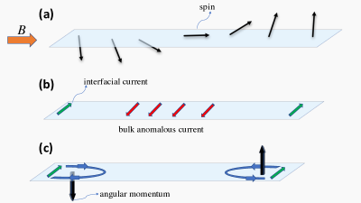
Figure 1: Schematically description of the magnetic response in finite size superconductors in the presence of an in-plane field $B$. (a) Black arrows represents the deviation of the spin density, $\delta S$, from the Pauli spin. Because of the SOC and the finite size of the sample a transverse component of $\delta S$ is generated. (b) The spin-charge coupling due to the SOC induces bulk (red arrows) and edge (green arrows) charge supercurrents. (c) Due to the finite size of the sample the edge currents flow in close loops (blue), inducing an out-of-plane angular momentum (black arrows).

In addition to the finite spin response at $T=0$, the SOC in superconductors also leads to the spin-galvanic effect, that is, a creation of charge currents by a Zeeman field Yip (2002); Dimitrova and Feigel?Man (2007); Edelstein (2005); Konschelle et al. (2015). In the stripe geometry (see middle panels of Fig. 2) the so called anomalous charge current is induced in $y$-direction, $j_{y}^{an}=(\theta/m)(\partial_{x}\delta S^{z}-2\alpha\delta S^{x})$ Tokatly (2017), where $\theta=2D\tau\alpha^{2}$ is a dimensionless parameter which in normal systems describes the spin-charge conversionSanz-Fernández et al. (2019). Within the diffusive approximation it is a small parameter which we treat perturbatively. Here $\delta S^{a}$ is obtained by substituting the solution of Eqs. (6)-(7) into Eq. (3). This results in

$$j_{y}^{an} = -4\pi\theta\frac{TN_{F}}{m}\sum_{\omega}\frac{\Delta^{2}}{E^{2}}\left(\partial_{x}\delta Q^{z}-2\alpha\delta Q^{x}-2\alpha Q_{b}^{x}\right)$$ (9)

$$\equiv j^{an}_{edge}(x)+j^{an}_{b}\;.$$

In the second line we identify two contributions to the anomalous current: the bulk contribution $j^{an}_{b}$, widely studied in homogeneous superconductors Yip (2002); Dimitrova and Feigel?Man (2007); Edelstein (1995); Konschelle et al. (2015) and given by the last term in the brackets in the first line and (red arrows in middle panels in Fig. 2), and the boundary contribution $j^{an}_{edge}$, determined by the first two terms. The latter are localized at the edges of the sample within the scale of superconducting coherence length (green arrows in middle panels of Fig. 2). In the geometry under consideration, the "bulk" contribution to the current is finite only for fields applied across the stripe ($x$-direction).

The spatial dependence of the charge current density is shown on Fig. 2 b and d for fields in $x$- and $z$-direction, respectively. Because of zero spin-current condition, Eq. (8), the charge current of Eq. (9) also vanishes at the boundaries. When the field is applied in $x$-direction, Fig. 2b, both, the bulk and edge contributions, are finite. The maximal value of the total current is the "bulk" value reached deeply inside the sample, away from the edges. The spatial distribution of the current is symmetric and the net current through the stripe is non-zero. In contrast, if the field is applied in $z$-direction, Fig. 2d, there is no bulk contribution, because $Q_{b}^{z}$ does not contribute to the current, see Eq. (9). Only edge currents, opposite on opposite sides, appear. Clearly in this case the total charge current vanishes.

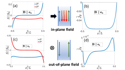
Figure 2: Spin density (panels a,c), and charge current density (panels b,d), induced by an in-plane (a-b) and out-of plane field (c-d), for $\alpha\xi_{0}=0.2$, $L=10\xi_{0}$. The middle panels show schematically the corresponding bulk (red arrows) and edge currents (green arrows)

The above results apply for an infinite superconducting stripe, and whether the obtained currents may exist in real finite systems depends on transverse boundary conditions. For example, if a finite stripe is wrapped in a cylinder, periodic boundary conditions indeed allow for the above current patterns when the field is applied along the the cylinder axis Dimitrova and Feigel?Man (2007). Here we consider a more experimentally relevant situation: a finite 2D superconductor of rectangular shape, which occupies the region $|x|<L/2$ and $|y|<W/2$ (see Fig. 3). The charge current through all boundaries must vanish. For out-of-plane field this condition is trivially satisfied by closing the boundary streamlines, which generates a circulating edge current. More interesting is the case of in-plane field. In this case the anomalous current has the same direction at both edges, Fig. 2(b), and as sketched in Fig. 2(c) one expects generation of closed streamlines at each edge.

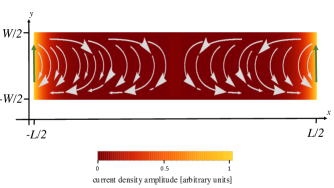
Figure 3: The current flow in a finite 2D superconductor with SOC when the field is applied in $x$-direction. The green arrows represents the edge contributions to the anomalous SH-current. The color-scale shows the decay of the current amplitude away from the interface.

Specifically, the total charge current in the superconductor reads,

$${\bf j}=\delta(z)\left[\frac{en_{s}}{2m}\left(\nabla\varphi-\frac{e}{c}{\bf A}\right)+j^{an}(x)\hat{\bf y}\right]\;,$$ (10)

where $n_{s}$ is the superfluid density in the 2D strip. The superconducting phase $\varphi(x,y)$ and the vector potential ${\bf A}({\bf r})$ are determined, respectivelly, by the continuity equation and the Maxwell equation,

$$\nabla\cdot{\bf j}=0\quad\text{and}\quad\nabla^{2}{\bf A}=-\frac{4\pi}{c}{\bf j}\;,$$ (11)

which should be solved with the zero-current condition at the edges, ${\bf n}\cdot{\bf j}|_{edge}=0$, where ${\bf n}$ is a unit vector normal to the edges of the sample. We assume that $n_{s}$ is homogeneous within the strip. Then, by choosing the gauge with $\nabla\cdot{\bf A}=0$, the continuity equation is reduced to the 2D Laplace equation for the phase, $\nabla^{2}\varphi=0$.

In the problem defined by Eqs. (10)-(11) one identifies three length scales: (i) a mesoscopic scale of the order of the coherence length $\xi_{s}$, over which the anomalous current $j^{an}(x)$ decays away from the edges, (ii) the Pearl length $\Lambda=mc^{2}/4\pi e^{2}n_{s}$ that is the scale controlling Meissner effect in 2D superconductors, and (iii) the sample geometry scales $W$, $L$. In the following we consider the typical situation when $\xi_{s}\ll\Lambda,W,L$ and analyze the current distribution in a narrow strip with $W\ll L$. In this case the anamolaous current in Eq. (10) can be written as $j^{an}(x)=I_{y}^{edge}\big{[}\delta(x+L/2)+\delta(x-L/2)\big{]}$, and the currents near opposite edges at $x=\pm L/2$ can be treated independently.

The current streamlines are sketeched in Fig. 3. Whereas the anomalous current is strongly localized at the edges (green arrows in Fig. 3), the counterflow supercurrent compensating the anomalous one, decays over a macroscopic scale determined by the width of the sample and/or the Pearl length $\Lambda$. If $W\ll\Lambda$, one can neglect ${\bf A}$ in Eq. (10) and the problem can be solved using the procedure described in Refs. Borge and Tokatly (2019); Sanz-Fernández et al. (2019). In this limit the counterflow decays exponentially over the scale $W$, and sufficiently far from the edges it takes the form,

$$(j_{x},\,j_{y})\propto I_{y}^{edge}\frac{e^{-\frac{\pi|x\pm L/2|}{2W}}}{W}\left(\sin\frac{\pi y}{2W},\,\cos\frac{\pi y}{2W}\right)$$ (12)

In the opposite limit of $W\gg\Lambda$ one can neglect the corner effects and apply the method of images and conformal mapping norris ; zeldov to compute screening supercurrents induced by an external current filament at the edge of 2D superconducting half-plane. This gives a power-law asymptotic decay of the counterflow supercurrent,

$$j_{y}\propto I_{y}^{edge}\sqrt{\Lambda}|x\pm L/2|^{-3/2}.$$ (13)

The total current generates a finite orbital angular momentum ${\cal L}_{z}$ at each edge, see Fig. 1c, which is computed from the general definition ${\cal L}_{z}=m\int\int dxdy(xj_{y}-yj_{x})/2$ and Eqs. (12) and (13)

$${\cal L}_{z}\propto-mf(W)I_{y}^{edge}\;,$$ (14)

where $f(W)=W^{2}$ in the limit $W\ll\Lambda$ and $f(W)=W^{3/2}\sqrt{\Lambda}$ when $W\gg\Lambda$ Note (6). The total magnetic moment is given by ${\cal M}_{z}=\mu_{B}({{\cal L}_{z}}/{\hbar}+{{\cal S}_{z}})$, where $\mu_{B}$ is the Bohr magneton . The total spin angular momentum accumulated at the edge is obtained by integrating the $z$-component of the spin, Eq. (3), ${\cal S}_{z}=\int_{-L/2}^{0}\delta S^{z}(x)dx$. Analytical expressions for both spin and orbital angular momenta at $T=0$ can be found in two cases NoteSM

$${\cal S}_{z}\propto-N_{F}h_{x}W\xi_{0}\begin{cases}\xi_{0}\alpha,&\text{for $\xi_{0}\alpha\ll 1$}\\ (\alpha\xi_{0})^{-3},&\text{for $\xi_{0}\alpha\gg 1$}\;,\end{cases}\\$$ (15)

and

$${\cal L}_{z}\propto-N_{F}h_{x}\theta f(W)\begin{cases}\xi_{0}\alpha,&\text{for $\xi_{0}\alpha\ll 1$}\\ (\xi_{0}\alpha)^{-4}\ln(\xi_{0}\alpha),&\text{for $\xi_{0}\alpha\gg 1$}\end{cases}\;$$ (16)

with $\xi_{0}=\sqrt{D/2\Delta}$. Both contributions have the same sign. The spin angular momentum scales with $W$, while ${\cal L}_{z}$ scales with $W^{2}$ or $W^{3/2}$ depending on the ratio $W/\Lambda$, and therefore dominates in macroscopic samples.

In conclusion, we present the theory of the magnetic response of finite size Rashba superconductors. When the field is applied in-plane, on the one hand, a finite out-of-plane spin polarization localized at the edge of the sample on the scale of superconducting coherence length appears. On the other hand, the SOC also leads to supercurrents circulating in the sample. Both the spin and the orbital momentum of supercurrents contribute to the total magnetic moment, which is induced at the edges and can be measured by state-of-the-art magnetic sensorsGranata and Vettoliere (2016); Maletinsky et al. (2012). Whereas the contribution from the spin angular momentum scales with the width $W$ of a rectangular stripe, the contribution from the currents scales with $W^{\gamma}$, with $\gamma>1$ and therefore dominates in large samples. There are several superconducting materials with Rashba SOC in which our findings can be verified. These range from Pb and Tl-Pb monolayers Qin et al. (2009); Sekihara et al. (2013); Brun et al. (2014); Matetskiy et al. (2015), to thin MoS₂, NbRe, $\beta$-Bi₂Pd films Yuan et al. (2014); Cirillo et al. (2016); Lv et al. (2017), and 2D superconductivity at the LaAlO₃/SrTiO₃ interface Dikin et al. (2011); Bert et al. (2011); Kalisky et al. (2012); Hurand et al. (2015). A particular interesting system has been studied recently moodera2020 . It consists of EuS grown on top of Au (111) surface which is proximitized by an adjacent superconductor. According to our theory, the exchange field induced by EuS, together with the large Rashba SOC in the Au 2D interface band, should lead to the transverse edge magnetization and edge supercurrents even in the absence of an external applied field.

Acknowledgements.- We acknowledge funding by the Spanish Ministerio de Ciencia, Innovación y Universidades (MICINN) (Projects No. FIS2016-79464-P and No. FIS2017-82804-P), by Grupos Consolidados UPV/EHU del Gobierno Vasco (Grant No. IT1249-19), and by EU’s Horizon 2020 research and innovation program under Grant Agreement No. 800923 (SUPERTED).

References

- Uchihashi (2016) T. Uchihashi, Superconductor Science and Technology 30, 013002 (2016).
- Saito et al. (2017) Y. Saito, T. Nojima, and Y. Iwasa, Nature Reviews Materials 2, 16094 (2017).
- Saito et al. (2016) Y. Saito, Y. Nakamura, M. S. Bahramy, Y. Kohama, J. Ye, Y. Kasahara, Y. Nakagawa, M. Onga, M. Tokunaga, T. Nojima, et al., Nature Physics 12, 144 (2016).
- Lu et al. (2015) J. Lu, O. Zheliuk, I. Leermakers, N. F. Yuan, U. Zeitler, K. T. Law, and J. Ye, Science 350, 1353 (2015).
- Gruznev et al. (2014) D. V. Gruznev, L. V. Bondarenko, A. V. Matetskiy, A. A. Yakovlev, A. Y. Tupchaya, S. V. Eremeev, E. V. Chulkov, J.-P. Chou, C.-M. Wei, M.-Y. Lai, et al., Scientific reports 4, 4742 (2014).
- Sekihara et al. (2013) T. Sekihara, R. Masutomi, and T. Okamoto, Physical review letters 111, 057005 (2013).
- Ménard et al. (2017) G. C. Ménard, S. Guissart, C. Brun, R. T. Leriche, M. Trif, F. Debontridder, D. Demaille, D. Roditchev, P. Simon, and T. Cren, Nature communications 8, 2040 (2017).
- Edelstein (1989) V. Edelstein, Soviet Physics-JETP (English Translation) 68, 1244 (1989).
- Edelstein (1995) V. M. Edelstein, Physical review letters 75, 2004 (1995).
- Edelstein (1996) V. M. Edelstein, Journal of Physics: Condensed Matter 8, 339 (1996).
- Yip (2002) S. Yip, Physical Review B 65, 144508 (2002).
- Gor’kov and Rashba (2001) L. P. Gor’kov and E. I. Rashba, Phys. Rev. Lett. 87, 037004 (2001).
- Frigeri et al. (2004) P. Frigeri, D. Agterberg, and M. Sigrist, New Journal of Physics 6, 115 (2004).
- Edelstein (2008) V. M. Edelstein, Physical Review B 78, 094514 (2008).
- Agterberg and Kaur (2007) D. Agterberg and R. Kaur, Physical Review B 75, 064511 (2007).
- Dimitrova and Feigelman (2003) O. V. Dimitrova and M. V. Feigelman, Journal of Experimental and Theoretical Physics Letters 78, 637 (2003).
- Dimitrova and Feigel?Man (2007) O. Dimitrova and M. Feigel?Man, Physical Review B 76, 014522 (2007).
- Pershoguba et al. (2015) S. S. Pershoguba, K. Björnson, A. M. Black-Schaffer, and A. V. Balatsky, Phys. Rev. Lett. 115, 116602 (2015).
- Mal’shukov (2016) A. G. Mal’shukov, Phys. Rev. B 93, 054511 (2016).
- Konschelle et al. (2015) F. Konschelle, I. V. Tokatly, and F. S. Bergeret, Phys. Rev. B 92, 125443 (2015), arXiv:1506.02977 .
- Edelstein (2003) V. M. Edelstein, Physical Review B 67, 020505 (2003).
- Note (1) In our notation has dimensions of momentum and it is proportional to the usual Rashba constant . Throughout the article we choose the -axis as the axis perpendicular to the superconductor plane.
- Abrikosov and Gor’kov (1962) A. A. Abrikosov and L. P. Gor’kov, Sov. Phys. JETP. 15, 752 (1962).
- (24) I. V. Tokatly, B. Bujnowski, and F. S. Bergeret, Phys. Rev. B 100, 214422 (2019), arXiv:1901.07890 (2019).
- Eilenberger (1968) G. Eilenberger, Zeitschrift für Physik 214, 195 (1968).
- Larkin and Ovchinnikov (1969) A. Larkin and Y. N. Ovchinnikov, Sov Phys JETP 28, 1200 (1969).
- Bergeret et al. (2005) F. S. Bergeret, A. F. Volkov, and K. B. Efetov, Rev. Mod. Phys. 77, 1321 (2005), arXiv:0506047 [cond-mat] .
- Bergeret and Tokatly (2013) F. S. Bergeret and I. V. Tokatly, Physical Review Letters 110, 117003 (2013), arXiv:1211.3084 .
- Bergeret and Tokatly (2014) F. S. Bergeret and I. V. Tokatly, Physical Review B 89, 134517 (2014), arXiv:1402.1025 .
- Note (2) If the magnetic field has a component out-of-plane one should include in Eq. (1) the usual U(1) vector potential which leads to orbital effects. Here we are interesting in the spin-magnetic response and neglect orbital terms.
- Note (3) In deriving Eq. (2) we used the linearized normalization condition .
- Note (4) The deviation from the Pauli response, , is determined by , where , and is the density of states at the Fermi level. In the normal state and therefore the generated magnetic moment is . In the superconducting state at zero temperature and zero SOC and hence the total magnetization is zero.
- Tokatly (2017) I. V. Tokatly, Physical Review B 96, 060502 (2017).
- Edelstein (2005) V. M. Edelstein, Physical Review B 72, 172501 (2005).
- Sanz-Fernández et al. (2019) C. Sanz-Fernández, J. Borge, I. V. Tokatly, and F. S. Bergeret, arXiv preprint arXiv:1907.11688 (2019).
- Borge and Tokatly (2019) J. Borge and I. V. Tokatly, Physical Review B 99, 241401 (2019)
- (37) W. T. Norris, J. Phys. D 3, 489 (1970).
- (38) E. Zeldov, J. R. Clem, M. McElfresh, and M. Darwin, Phys. Rev. B 49, 9802 (1994).
- (39) See Supplementary Material for details.
- Note (6) In the limit , by substituting Eq. (13) into the integral we find that it formally diverges as for large . The natural cut-off is the width of the stripe such that . The integration over provides the additional factor which results in Eq. (14).
- Note (5) The spin magnetic moment is given by
- Granata and Vettoliere (2016) C. Granata and A. Vettoliere, Physics Reports 614, 1 (2016).
- Maletinsky et al. (2012) P. Maletinsky, S. Hong, M. S. Grinolds, B. Hausmann, M. D. Lukin, R. L. Walsworth, M. Loncar, and A. Yacoby, Nature nanotechnology 7, 320 (2012).
- Qin et al. (2009) S. Qin, J. Kim, Q. Niu, and C.-K. Shih, Science 324, 1314 (2009).
- Brun et al. (2014) C. Brun, T. Cren, V. Cherkez, F. Debontridder, S. Pons, D. Fokin, M. Tringides, S. Bozhko, L. Ioffe, B. Altshuler, et al., Nature Physics 10, 444 (2014).
- Matetskiy et al. (2015) A. Matetskiy, S. Ichinokura, L. Bondarenko, A. Tupchaya, D. Gruznev, A. Zotov, A. Saranin, R. Hobara, A. Takayama, and S. Hasegawa, Physical review letters 115, 147003 (2015).
- Yuan et al. (2014) N. F. Yuan, K. F. Mak, and K. Law, Physical review letters 113, 097001 (2014).
- Cirillo et al. (2016) C. Cirillo, G. Carapella, M. Salvato, R. Arpaia, M. Caputo, and C. Attanasio, Physical Review B 94, 104512 (2016).
- Lv et al. (2017) Y.-F. Lv, W.-L. Wang, Y.-M. Zhang, H. Ding, W. Li, L. Wang, K. He, C.-L. Song, X.-C. Ma, and Q.-K. Xue, Science bulletin 62, 852 (2017).
- Dikin et al. (2011) D. Dikin, M. Mehta, C. Bark, C. Folkman, C. Eom, and V. Chandrasekhar, Physical Review Letters 107, 056802 (2011).
- Bert et al. (2011) J. A. Bert, B. Kalisky, C. Bell, M. Kim, Y. Hikita, H. Y. Hwang, and K. A. Moler, Nature physics 7, 767 (2011).
- Kalisky et al. (2012) B. Kalisky, J. A. Bert, B. B. Klopfer, C. Bell, H. K. Sato, M. Hosoda, Y. Hikita, H. Y. Hwang, and K. A. Moler, Nature communications 3, 922 (2012).
- Hurand et al. (2015) S. Hurand, A. Jouan, C. Feuillet-Palma, G. Singh, J. Biscaras, E. Lesne, N. Reyren, A. Barthélémy, M. Bibes, J. Villegas, et al., Scientific reports 5, 12751 (2015).
- (54) S. Manna, P. Wei, Y. Xie, K. T. Law, P. A. Lee, J. S. Moodera, Proceedings of the National Academy of Sciences, 117, 8775 (2020).