A Supervised Learning Algorithm for Multilayer Spiking Neural Networks Based on Temporal Coding Toward Energy-Efficient VLSI Processor Design

Abstract

Spiking neural networks (SNNs) are brain-inspired mathematical models with the ability to process information in the form of spikes. SNNs are expected to provide not only new machine-learning algorithms, but also energy-efficient computational models when implemented in VLSI circuits. In this paper, we propose a novel supervised learning algorithm for SNNs based on temporal coding. A spiking neuron in this algorithm is designed to facilitate analog VLSI implementations with analog resistive memory, by which ultra-high energy efficiency can be achieved. We also propose several techniques to improve the performance on a recognition task, and show that the classification accuracy of the proposed algorithm is as high as that of the state-of-the-art temporal coding SNN algorithms on the MNIST dataset. Finally, we discuss the robustness of the proposed SNNs against variations that arise from the device manufacturing process and are unavoidable in analog VLSI implementation. We also propose a technique to suppress the effects of variations in the manufacturing process on the recognition performance.

1 Introduction

Machine learning is a paradigm according to which algorithms perform tasks by learning from data instead of exploiting domain knowledge. Recently, machine-learning algorithms that employ artificial neural networks (ANNs) have been attracting much interest from researchers and engineers in diverse fields owing to their astonishing performance on various tasks such as image recognition, natural language processing, and time series forecasting [1, 2]. These machine-learning algorithms are known as deep learning because of the characteristic multilayer structures of ANNs. In deep learning, stochastic gradient descent (SGD) and back propagation (BP) are important techniques that enable multilayer ANNs to perform effective learning [3, 4]. In addition, recent advances in algorithms such as convolutional neural networks (CNNs) [5] and skip connections[6] have led to the success of deep learning. Moreover, the evolution of very large-scale integration (VLSI) technologies, such as Moore’s law [7] and Dennard scaling[8], have enabled deep learning to be implemented in real-world applications.

However, the computational burden of deep learning often hinders its application in the real world. Therefore, researchers and engineers often use high-performance processors such as graphical processing units, tensor processing units[9], and application-specific integrated circuits (ASICs)[10] to compensate for this shortcoming. Despite these developments, it remains difficult to enable the learning to converge in an acceptable time, or to perform the tasks in real time. This is even more difficult when performing tasks with processors placed near the end-users (edge computing) owing to the limited battery capacity. Therefore, for edge computing, high computational energy efficiency is required.

In this regard, finding a solution for the energy-efficiency problem by looking toward the human brain would only seem natural, because the human brain is capable of processing complex information in real time by consuming only 20-30 W of energy. An ANN is mostly a mathematical model inspired by the physiological observation of spike frequencies in biological neurons, whereas a spiking neural network (SNN) is a mathematical model that is directly concerned with the spike generation [11]. Therefore, SNNs would be expected to perform tasks in a way similar to the brain with low energy consumption. Until recently, SNNs did not perform as well as ANNs on tasks such as image recognition. However, it has been shown that the performance of SNNs could reach that of ANNs by exploiting the techniques used in deep learning (multilayer structures, SGD, BP, etc.)[12, 13]. Thus, it seems reasonable to find a way to really improve the energy efficiency of SNNs. In fact, not only have SNNs demonstrated their high algorithmic performance but also their advantages in terms of energy efficiency especially when implemented in ASICs by exploiting the asynchronous property and binary (spike) communications [14]. Many research groups have manufactured various types of ASICs for SNNs, which include, for example, mixed-signal ASICs[15, 16, 17, 18], and fully digital ASICs [19, 20]. Other ASICs were also reported [21, 22]. These ASICs are able to execute SNNs with complex and flexible networks in a highly energy efficient manner. However, it is still unclear whether ASICs for SNNs are more energy efficient per operation or per task than ASICs for ANNs. This comparison is blurred by a common bottleneck preventing computational energy efficiency, which is caused by data movement between processors and memory [23]. Because of this common bottleneck, the advantages of employing SNNs in a hardware implementation such as the asynchronous property and spike communications are hardly visible in terms of the computational energy efficiency of ASICs. One promising approach to overcome this bottleneck is in-memory computing.

In-memory computing is a concept that involves performing the computing where the memorized data are located [24]. Especially, in-memory computing schemes that use analog resistive memory have being attracting hardware researchers’ attention [25, 26, 27]. Analog resistive memory stores information in the form of resistance. The application of voltage across the two terminals of an analog resistive memory cell results in an electric current, which is proportional to the voltage, and which flows through the memory cell by obeying Ohm’s law. Currents flowing through memory cells can easily be summed up on the basis of Kirchhoff’s current law. Note that this computing scheme does not require information to be stored elsewhere (e.g., static random access memory or dynamic random access memory). Based on the above principle, computing such as matrix-vector multiplications (MVMs) can be performed in a highly energy efficient way.

This motivated us to propose a novel supervised learning algorithm for multilayer SNNs to achieve high algorithmic performance and high energy efficiency. It is also possible to implement our algorithm in VLSI circuits with analog resistive memory. Our algorithm is based on the following ideas: (i) SNNs are composed of spiking neuron models which facilitate VLSI implementations; (ii) SNNs are trained with a temporal coding scheme, thereby enabling SNNs to perform tasks with fewer spikes than SNNs based on rate coding. We also propose novel learning techniques to improve the learning performance and evaluate the performance on the MNIST dataset. Furthermore, for real VLSI implementations, robustness against manufacturing variations in devices is crucial. Therefore, we investigated the effects of these manufacturing variations on the learning performance of the proposed algorithm. In addition, we propose a technique to suppress the effect of manufacturing variations.

This paper consists of the following sections: section 2 describes related work; section 3 proposes an SNN and its learning algorithm; section 4 introduces the experimental setup for evaluating the algorithm on the MNIST dataset, and for investigating the effects of manufacturing variations; section 5 presents the experimental results; section 6 concludes this paper.

2 Related Work

2.1 Supervised learning algorithms for multilayer SNNs

Figure 1: Different representations of information in SNNs. The arrows represent the directions of information propagation. The widths of spikes do not carry information. (a) Information is contained in the spike frequency (rate coding). (b) Information is contained in the spike timing (temporal coding).

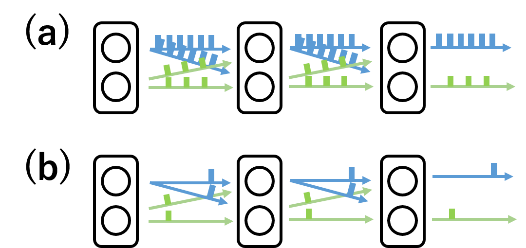
A number of studies have shown that multilayer SNNs can be trained with the BP technique [12, 13, 28]. The application of the BP to SNNs is not straightforward as in the case of ANNs because SNNs have non-differentiable processes such as spike generations. Furthermore, the dynamics and the learning performance depend on the coding schemes of SNNs. Fig. 1 shows SNNs based on two different coding schemes: rate coding and temporal coding. In rate coding, information is contained in the spike frequency of neurons, whereas in temporal coding, information is contained in the spike timing of neurons [29].

In rate coding, BP algorithms can be obtained by approximations such as linear neuron approximation [30], and by considering spike generation as a probabilistic process [31]. In [32, 33, 28], the BP algorithms were obtained by using the derivative of the membrane potential with respect to time. In addition, it has been shown that trained ANNs can be converted into rate-coding-based SNNs [34, 35]. However, these algorithms need to average a number of spikes to propagate information forward or backward. Because the energy consumption of ASICs increases as the number of spikes increases, performing tasks with fewer spikes is preferable.

Temporal coding enables SNNs to perform tasks with fewer spikes compared to rate coding. SpikeProp is the first algorithm that enabled multilayer SNNs to learn by using temporal coding[36]. SpikeProp obtains the BP algorithm by directly differentiating spike timing with respect to weights. Mostafa [37] improved the learning performance of SNNs in temporal coding on recognition tasks by using non-leaky spiking neurons. Comsa et al. [38] used an alpha synaptic function and employed an evolutionary algorithm to search for the hyperparameter to improve the learning performance.

In this paper, we propose a supervised learning algorithm for SNNs based on temporal coding, which is similar to those mentioned above [37, 38]. The novelties of our work are as follows: we use a different neuron model to simplify the hardware implementation and modify the learning algorithm to improve the learning performance.

2.2 Computing with analog resistive memory

Analog resistive memory such as resistive RAM and phase change memory is considered important building blocks for next-generation artificial-intelligence processors [25, 26, 27]. Many research groups have already designed circuits with analog resistive memory to efficiently compute MVMs [39, 40, 41, 42, 43]. Among various VLSI implementations with analog resistive memory, circuits that process information by using the timing of electronic pulses are expected to be advantageous in terms of energy efficiency because of their simple implementation [43, 44, 45, 46, 47, 48, 49, 50, 51]. For example, circuits using the timing difference between two pulses [48, 49] and those using the pulse-width difference between two pulses [50, 51] are able to compute MVMs efficiently. Nandakumar et al. [52] developed circuits with phase change memory that is capable of computing single-layer SNNs based on rate coding.

In this paper, we show that SNNs based on temporal coding can be straightforwardly mapped to the above VLSI implementation schemes.

3 Methods

This section introduces our proposed SNNs and their learning algorithms. The SNNs described here are feedforward networks of spiking neurons as shown in Fig. 1(b), where spikes propagate from one layer to the next layer without skipping layers. The SNNs are to be trained such that the network can convert a given input spike pattern into a specific output spike pattern. We also present several examples of VLSI implementations of the SNNs where analog resistive memory is used as network weights.

3.1 Models

Figure 2: (a) Schematic diagram of a multilayer SNN. The $k$th neuron in the $l$th layer receives spikes from neurons in the $(l-1)$th layer at $t_{1}^{(l-1)},t_{2}^{(l-1)},t_{3}^{(l-1)}$, and fires at $t_{k}^{(l)}$. Then, a spike is sent to neurons in the subsequent layer. (b) Schematic diagram of time evolution of the membrane potential $v_{k}^{(l)}$ of the $k$th neuron in the $l$th layer.

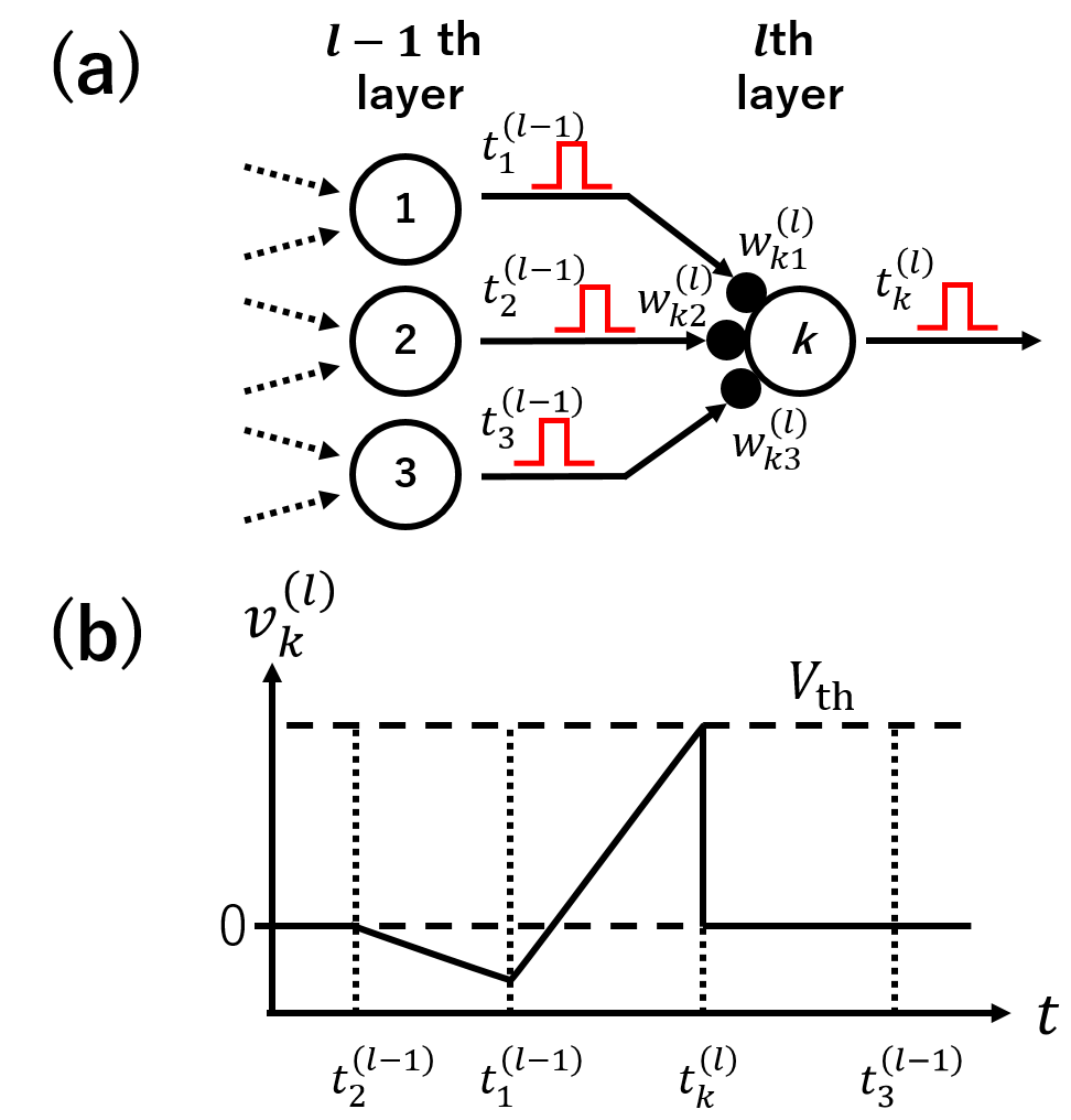
The time evolution of the membrane potential of a spiking neuron that we employed is given by

$$\frac{d}{dt}v_{i}^{(l)}(t) =\sum_{j=1}^{N^{(l-1)}}w_{ij}^{(l)}\theta(t-t_{j}^{(l-1)})$$ (1)

$$\theta(x) =\begin{cases}0,&~{}(x<0)\\ 1,&~{}(x\geq 0)\end{cases}$$ (2)

where we define $v_{i}^{(l)}(t)$ as the membrane potential of the $i$th spiking neuron in the $l$th layer, and define $t^{(l)}_{i}$ as the spike timing generated by the same neuron to the present input pattern. We define $w_{ij}^{(l)}$ as the weight of the connection from the $j$th neuron in the $(l-1)$th layer to the $i$th neuron in the $l$th layer. $N^{(l)}$ is the number of neurons constituting the $l$th layer. The zeroth layer and the $M$th layer are referred to as the input and output layers, respectively. The other layers are hidden layers. This network is an $M$-layer SNN.

The analytical solution of (1) is given by

$$v_{i}^{(l)}(t)=\sum_{j=1}^{N^{(l-1)}}w_{ij}^{(l)}(t-t_{j}^{(l-1)})\theta(t-t_{j}^{(l-1)}).$$ (3)

The neuron generates (fires) a spike when its membrane potential reaches the firing threshold $V_{\text{th}}$. Then, the membrane potential is fixed to the reset voltage ($v_{i}^{(l)}=0$), which prevents the neuron from firing twice for a given input spike pattern. Fig. 2(b) shows a schematic diagram to indicate the dependence of the evolution of the membrane potential on the timing of received spikes and the connection weights.

The timing of spikes can be obtained as follows. The spike timing $t_{i}^{(l)}$ satisfies the equation

$$V_{\text{th}}=\sum_{j\in\Gamma_{i}^{(l)}}w_{ij}^{(l)}(t_{i}^{(l)}-t_{j}^{(l-1)})$$ (4)

where $\Gamma_{i}^{(l)}$ is a set of indices of neurons in the $(l-1)$th layer that sends spikes before the $i$th neuron in the $l$th layer fires. With (4), we obtain the spike timing as follows:

$$t_{i}^{(l)} =\frac{V_{\text{th}}+\sum_{j\in\Gamma_{i}^{(l)}}w_{ij}^{(l)}t_{j}^{(l-1)}}{\sum_{j\in\Gamma_{i}^{(l)}}w_{ij}^{(l)}}.$$ (5)

3.2 Supervised learning of SNNs

For the supervised learning of SNNs, we define the following functions

$$C(\bm{t}^{(M)},\bm{\kappa};\bm{w}) :=L(\bm{t}^{(M)},\bm{\kappa};\bm{w})+\frac{\gamma}{2}R(\bm{t}^{(M)})$$ (6)

$$L(\bm{t}^{(M)},\bm{\kappa};\bm{w}) :=-\sum_{i=1}^{N^{(M)}}\kappa_{i}\ln\left(S_{i}(\bm{t}^{(M)})\right)$$ (7)

$$S_{i}(\bm{t}^{(M)}) :=\frac{\exp\left(-t_{i}^{(M)}\right)}{\sum_{j=1}^{N^{(M)}}\exp\left(-t_{j}^{(M)}\right)}$$ (8)

$$R(\bm{t}^{(M)}) :=\sum_{i=1}^{N^{(M)}}\left(t_{i}^{(M)}-t^{\text{(Ref)}}\right)^{2}$$ (9)

where $C(\cdot,\cdot;\cdot),~{}L(\cdot,\cdot;\cdot),~{}S_{i}(\cdot),\text{ and }R(\cdot)$ are the cost function, loss function, softmax function, and temporal penalty term, respectively. Teacher labels are represented as a vector $\bm{\kappa}$ such that $\kappa_{i}$ is 1 when the $i$th label is given, and 0, otherwise. The weights of the entire network are represented as a vector $\bm{w}$. The temporal penalty term $R(\bm{t}^{(M)})$ is defined by the total difference between the spike timing of the output neurons $\bm{t}^{(M)}$ and the timing of a reference spike $t^{\text{(Ref)}}$. Note that $\bm{t}^{(M)}$ is the vector of spike timing of the neurons in the output layer. As explained later, the temporal penalty is intended to circumvent learning difficulties. The coefficient $\gamma(>0)$ controls the effect of the temporal penalty term.

The network is trained by updating the weights by using SGD on a dataset as follows:

$$\Delta w_{jk}^{(l)}=-\eta\frac{\partial C(\bm{t}^{(M)},\bm{\kappa};\bm{w})}{\partial w_{jk}^{(l)}}$$ (10)

where $\Delta w_{jk}^{(l)}$ is the update of $w_{jk}^{(l)}$ and $\eta(>0)$ is the learning rate. The derivative of the cost function with respect to weights is given by

$$\frac{\partial C}{\partial w_{ij}^{(l)}}=\frac{\partial t_{i}^{(l)}}{\partial w_{ij}^{(l)}}\delta_{i}^{(l)}$$ (11)

where we define the propagation error $\delta_{i}^{(h)}$ as

$$\delta_{i}^{(h)}=\begin{cases}\sum_{k=1}^{N^{(h+1)}}\frac{\partial t_{k}^{(h+1)}}{\partial t_{i}^{(h)}}\delta_{k}^{(h+1)},\text{ for }h=1,2,\dots,M-1\\ \frac{\partial C}{\partial t_{i}^{(M)}},\text{ for }h=M.\end{cases}$$ (12)

By using the following derivatives

$$\frac{\partial t_{i}^{(l)}}{\partial w_{ij}^{(l)}} =-\frac{t_{i}^{(l)}-t_{j}^{(l-1)}}{\sum_{k\in\Gamma_{i}^{(l)}}w_{ik}^{(l)}}$$ (13)

$$\frac{\partial t_{i}^{(l)}}{\partial t_{j}^{(l-1)}} =\frac{w_{ij}^{(l)}}{\sum_{k\in\Gamma_{i}^{(l)}}w_{ik}^{(l)}}$$ (14)

$$\frac{\partial C}{\partial t_{i}^{(M)}} =\kappa_{i}-S_{i}+\gamma\left(t_{i}^{(M)}-t^{\text{(Ref)}}\right)$$ (15)

the updating difference (10) can be obtained.

The derivative of the cost function is rigorous unless a neuron ceases to fire because of the update. However, we found that the network experience two difficulties during training. These difficulties are related to destructively large weight updates and non-unique spike timing, respectively. The destructively large weight updates are caused by infinitesimal values in the denominator of (13) or (14). Our solution to prevent these unacceptable large weight updates is to redefine (13) and (14) as

$$\frac{\partial t_{i}^{(l)}}{\partial w_{ij}^{(l)}} =-\frac{t_{i}^{(l)}-t_{j}^{(l-1)}}{\epsilon+\sum_{k\in\Gamma_{i}^{(l)}}w_{ik}^{(l)}}$$ (16)

$$\frac{\partial t_{i}^{(l)}}{\partial t_{j}^{(l-1)}} =\frac{w_{ij}^{(l)}}{\epsilon+\sum_{k\in\Gamma_{i}^{(l)}}w_{ik}^{(l)}}$$ (17)

where $\epsilon$ is a positive constant.

Next, the loss function shown in (7) is invariant against an arbitrary value $\alpha$ such that

$$L(\bm{t}^{(M)},\bm{\kappa};\bm{w})=L(\bm{t}^{(M)}+\alpha\bm{I},\bm{\kappa};\bm{w})$$ (18)

where $\bm{I}\in\mathbb{R}^{N^{(M)}}$ is a vector of which the elements are all unity. Owing to its invariant nature, the loss function does not uniquely specify the timing of output spikes, which forces the timing of the output spike to become large, resulting in the disappearance of spikes. The temporal penalty term, which is introduced to solve this problem, enables the cost function to uniquely specify the timing of the output spike to approximate $t^{\text{(Ref)}}$ of the reference spike.

Here, we summarize the difference between our algorithm and the algorithms reported before [37, 38]. These previous studies were also concerned with the supervised learning of SNNs based on temporal coding. They used almost the same loss function like an exponential form of spike timing in [37]. Their approach to avoid the destructively large weight updates was to normalize the gradient when it became excessively large [37], or to clip the gradient to a fixed value [38]. We use a simple method (16) and (17), which can prevent the magnitude of the updated weights from becoming too large. They also reported the spike disappearance problem as explained above. Mostafa [37] avoided this problem by introducing a penalty term that increased the sum of values of weights and the $L2$ regularization term, but the two terms need to be balanced appropriately. Comsa et al. [38] also avoided this problem by adding a small penalty that increased the sum of weights when a neuron did not fire. On the other hand, we avoid this problem by introducing the temporal penalty term, which is a more direct way to stabilize the timing of an output spike. Our approach enhances the performance compared to that of Mostafa [37], and is slightly superior to that of Comsa et al. [38].

3.3 Deep learning with SNNs

Because the important properties of deep learning are sequential nonlinear transformations over layers and end-to-end learning, the proposed algorithm can be considered to be a form of deep learning. The proposed SNN processes information by converting the pattern of an input spike $\bm{t}^{(0)}$ in a layer-by-layer manner as follows:

$$\bm{t}^{(0)}\rightarrow\bm{t}^{(1)}\rightarrow\cdots\rightarrow\bm{t}^{(M)}$$ (19)

where $\bm{t}^{(l)}:=\{t_{1}^{(l)},t_{2}^{(l)},\dots,t_{N^{(l)}}^{(l)}\}$. Note that $t_{i}^{(l)}$ is considered to be a sufficiently large constant if the $i$th neuron in the $l$th layer does not fire at the end of the simulations. It is worth noting that the layer-to-layer nonlinear transformation in SNNs is different from that in ANNs. According to (5), the spike timing $t_{i}^{(l)}$ is a linear function of the presynaptic spike timing $t_{j}^{(l-1)}$ if $t_{i}^{(l)}>t_{j}^{(l-1)}$, whereas it does not depend on $t_{j}^{(l-1)}$ if $t_{i}^{(l)}\leq t_{j}^{(l-1)}$. This function seems to be similar to a rectified linear unit (ReLU)[53], which is commonly used as an activation function for ANNs. However, unlike ReLUs, the turning point, $t_{i}^{(l)}=t_{j}^{(l-1)}$, is determined by other spikes and their weights. In other words, the information is processed by using the timing order of spikes, which is the most unique characteristic of SNNs based on temporal coding.

3.4 Consideration of VLSI implementation

Figure 3: Examples of implementations of analog circuits of spiking neurons. Dashed squares are integrators, which convert summed currents into voltages: circuit implementation (a) with and (b) without operational amplifiers.

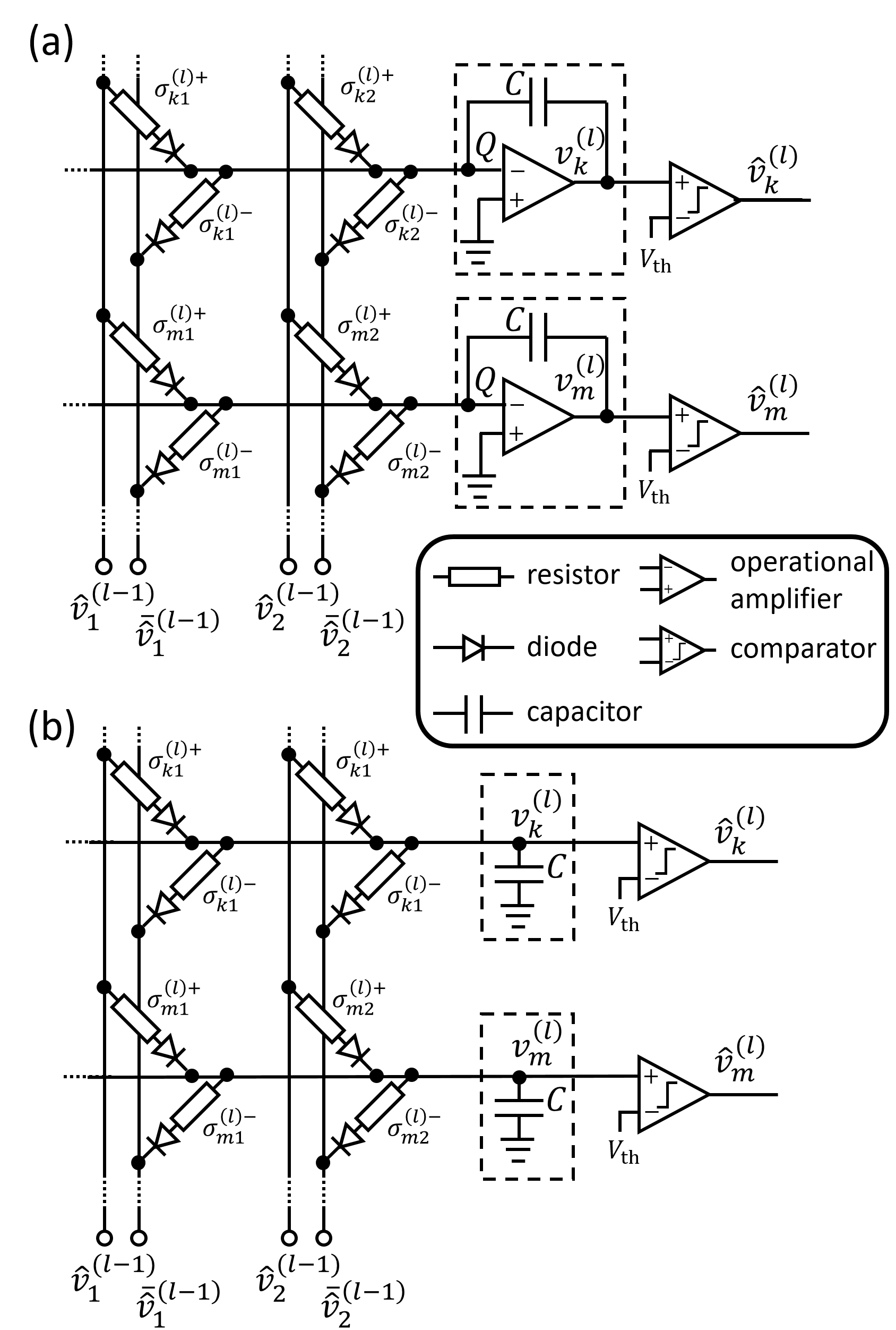
For analog VLSI implementations, the dynamics of SNNs must be physically realized in circuits that are carefully designed using either the nonlinear or linear properties of transistors. Here, we show that the time evolution of the membrane potential of neurons as expressed by (1) can be mapped to circuits with analog resistive memory in a simple and straightforward manner.

Fig. 3(a) shows an example of such implementations including the analog resistive memory, operational amplifiers, capacitors, and comparators. The membrane potential $v_{i}^{(l)}$ is represented as the voltage at the capacitor $C$, which is determined by the charge at the node $Q$. A spike is generated by a comparator when the membrane voltage exceeds the firing threshold voltage $V_{\text{th}}$. The existence of the spike is represented with the output voltage $\hat{v}_{i}^{(l)}$ and $\bar{\hat{v}}_{i}^{(l)}$ as follows:

$$\left(\hat{v}_{i}^{(l)}(t),\bar{\hat{v}}_{i}^{(l)}(t)\right)=\begin{cases}\left(V_{\text{pulse}}^{-},V_{\text{pulse}}^{+}\right),&~{}(t<t_{i}^{(l)})\\ \left(V_{\text{pulse}}^{+},V_{\text{pulse}}^{-}\right),&~{}(t\geq t_{i}^{(l)})\end{cases}$$ (20)

where $V_{\text{pulse}}^{\pm}$ are constants and $V_{\text{pulse}}^{-}<0<V_{\text{th}}<V_{\text{pulse}}^{+}$ is assumed.

In Fig. 3, $\sigma_{ij}^{(l)+}$ and $\sigma_{ij}^{(l)-}$ represent the conductance (the inverse of the resistance) from the $j$th neuron in the $(l-1)$th layer to the $i$th neuron in the $l$th layer. This combination can represent positive weights and negative weights as explained later. Currents flow through the conductance $\sigma_{ij}^{(l)\pm}$ to the $i$th neuron in the $l$th layer, which causes the membrane potential $v_{i}^{(l)}$ to change. It should be noted that, in Fig. 3(a), the voltage at node Q is virtually grounded because of the operational amplifiers. The time evolution of the membrane potential $v_{i}^{(l)}$ is obtained by Kirchhoff’s current law and Ohm’s law as follows:

$$C\frac{d}{dt}v_{i}^{(l)}(t)=\sum_{j=1}^{N^{(l-1)}}\left(\sigma_{ij}^{(l)+}V_{\text{pulse}}^{+}+\sigma_{ij}^{(l)-}V_{\text{pulse}}^{-}\right)\theta(t-t_{j}^{(l-1)}).$$ (21)

By setting $C=1$ and $\sigma_{ij}^{(l)+}V_{\text{pulse}}^{+}+\sigma_{ij}^{(l)-}V_{\text{pulse}}^{-}=w_{ij}^{(l)}$, (21) agrees with (1).

We introduce another simpler circuit configuration, as shown in Fig. 3(b), to allow us to investigate the effect of an approximation of the neuron model (1) on the learning performance. This circuit implementation is similar to that in [49], which was proposed for calculating vector-matrix operations. Because this circuit (Fig. 3(b)) uses no operational amplifiers, which often consume the largest amount of energy in analog circuits, this implementation is expected to be more energy efficient. Similar to (21), the time evolution of the membrane potential $v_{i}^{(l)}$ is performed by using Kirchhoff’s current law and the Ohm’s law as follows:

$$C\frac{d}{dt}v_{i}^{(l)}(t)= \sum_{j=1}^{N^{(l-1)}}\sigma_{ij}^{(l)+}(V_{\text{pulse}}^{+}-v_{i}^{(l)})\theta(t-t_{j}^{(l-1)})$$

$$+\sigma_{ij}^{(l)-}(V_{\text{pulse}}^{-}-v_{i}^{(l)})\theta(t-t_{j}^{(l-1)})$$

$$= \sum_{j=1}^{N^{(l-1)}}w_{ij}^{(l)}\delta_{w_{ij}^{(l)}\geq 0}\left(1-\frac{v_{i}^{(l)}}{V_{\text{pulse}}^{+}}\right)\theta(t-t_{j}^{(l-1)})$$

$$+w_{ij}^{(l)}\delta_{w_{ij}^{(l)}<0}\left(1-\frac{v_{i}^{(l)}}{V_{\text{pulse}}^{-}}\right)\theta(t-t_{j}^{(l-1)})$$

$$= \sum_{j=1}^{N^{(l-1)}}w_{ij}^{(l)}\left(1-v_{i}^{(l)}V_{\text{pulse}}^{ij}\right)\theta(t-t_{j}^{(l-1)})$$ (22)

where we define

$$\delta_{s} :=\begin{cases}0,\text{ if a condition $s$ is false}\\ 1,\text{ if a condition $s$ is true}\end{cases}$$ (23)

$$V_{\text{pulse}}^{ij} :=\frac{\delta_{w_{ij}^{(l)}\geq 0}}{V_{\text{pulse}}^{+}}+\frac{\delta_{w_{ij}^{(l)}<0}}{V_{\text{pulse}}^{-}}.$$ (24)

Note that the following relationships

$$\sigma_{ij}^{(l)+} =\frac{w_{ij}^{(l)}\delta_{w_{ij}^{(l)}\geq 0}}{V_{\text{pulse}}^{+}}~{}~{}~{}\sigma_{ij}^{(l)-}=\frac{w_{ij}^{(l)}\delta_{w_{ij}^{(l)}<0}}{V_{\text{pulse}}^{-}}$$ (25)

were used. By setting $C=1$ and letting $V_{\text{pulse}}^{ij}\rightarrow 0$, (22) converges to (1), where $V_{\text{pulse}}^{ij}\rightarrow 0$ is realized by $|V_{\text{pulse}}^{\pm}|\rightarrow\infty$. However, smaller values of $|V_{\text{pulse}}^{\pm}|$ are more preferable in terms of energy efficiency. The effects of the finite values of $|V_{\text{pulse}}^{\pm}|$ on the learning performance were not previously considered [49]. Thus, we investigated the effects by numerical simulations. Except when explicitly pointed out, simulations were conducted with the neuron model expressed by (1). Details of the simulation method and the learning methods for the neuron model expressed by (22) are provided in the appendix. We note that if current sources (field-effect transistors) are used instead of resistors, as employed by others [51], the time evolution equation becomes similar to (21) corresponding to the case of Fig. 3(a).

Finally, we explain the advantages of SNNs over time-domain circuits of ANNs[46, 50, 51, 49] in terms of the energy efficiency of circuits. First, the circuits of Marinella et al. [46] need Analog-to-Digital Converters (ADCs) to convert the signal for each layer of ANNs, which are known as energy-hungry processes. Actually, it is reported that ADCs were the energy bottleneck in the systems [46]. Circuit implementations requiring no ADCs were proposed [50, 51, 49]. These circuits compute the positive and negative weights independently, and subsequently take the difference of the two. As a result of the above principles, these circuits require two circuits to compute the positive and negative weights, and the dynamic range decreases significantly because the difference is taken (corresponding to digit loss in digital computing). The advantage of using SNNs over these circuits is that our circuits shown in Fig. 3 require no full ADCs because the input and output of the circuits consist of binary spikes, and that the circuits can compute the positive and negative weights at the same time.

4 Experimental setup

In this section, we describe the experimental setup for evaluating the learning performance of the proposed algorithm with the MNIST dataset[54]. We also present the experimental setup for evaluating the robustness of the algorithms against manufacturing variations in the devices, which are unavoidable in analog VLSI implementations. In all the experiments, we set $V_{\text{th}}=1$. We again note that neuron model (1) was used unless otherwise noted.

4.1 Model evaluation with MNIST dataset

The MNIST dataset [54] consists of 70,000 images of handwritten digits, each of which is represented as a $784~{}(=28\times 28)$-dimensional vector with a label of a corresponding integer (from 0 to 9). In our experiments, 60,000 images were used for training, and the remaining 10,000 images were used for testing, as in [54].

To process data in SNNs, the vector data are converted into spike patterns as follows: we normalize all the elements (pixels) of the vector $\bm{x}$ as $0\leq x_{i}\leq 1$. Then, the corresponding input spikes are generated at

$$t_{i}^{\text{(0)}}=\tau^{\text{(in)}}\left(1-x_{i}\right),\text{ if }x_{i}>0$$ (26)

where $\tau^{\text{(in)}}$ is the maximum time window of the input spikes, and was set at $5$ ms in our experiments. A spike is not generated when $x_{i}=0$. At the training phase, to improve the generalization performance, noise was introduced according to a Gaussian distribution $N(0,\sigma_{t})$ with zero mean and standard deviation $\sigma_{t}$.

4.2 Robustness against device manufacturing variations

In analog VLSI implementations, variations in the manufactured devices are unavoidable, and must be taken into account during circuit design. In this experiment, we investigated the effect of manufacturing variations on the learning performance, which has yet not been reported for SNNs based on temporal coding, to the best of our knowledge. To suppress these effects, we employed a learning technique that is described later.

In the VLSI implementations of Fig. 3(a) and Fig. 3(b), various parameters, such as weights, capacitance, spike delays, and firing threshold, need to be taken into account. Owing to the computational complexity, we investigated the effects of variations on the learning performance of only the firing threshold and spike delays in this study. We chose these two parameters because they affect the network dynamics in a different way: the firing threshold changes the generation timing of spikes, whereas the spike delays shift the arrival timing of spikes. The other parameters can be investigated in the same way we explained below. The remainder of this section describes the mathematical representations of the variations and then the evaluations of the effects of the variations.

First, we mathematically model the variations of the firing threshold $V_{\text{th}}$. We define the firing threshold of the $i$th neuron in the $l$th layer as $V_{\text{th}}^{(l,i)}$. For simplicity, we assume that the probability density distribution of the variation is a clipped Gaussian distribution as follows:

$$V_{\text{th}}^{(l,i)} =\max\left(\hat{V}_{\text{th}}^{(l,i)},0\right)$$ (27)

$$\hat{V}_{\text{th}}^{(l,i)} \sim N(V_{\text{th}},\sigma_{V_{\text{th}}})$$ (28)

where $N(V_{\text{th}},\sigma_{V_{\text{th}}})$ represents a Gaussian distribution with mean $V_{\text{th}}$ and standard deviation $\sigma_{V_{\text{th}}}$ and the operation ‘$\sim$’ means drawing a value from the distribution.

Figure 4: (a) Schematic diagram of the spike delays. Each connection has its own delay such as $\tau_{k1}^{(l)}$. (b) The probabilistic distribution of spike delays given by (29). Assuming that the mean $\tau_{\text{offset}}^{(l)}$ of the Gaussian distribution is much larger than the standard deviation $\sigma_{\tau}$, the probability of drawing negative values from (29) is negligible.

Second, we mathematically model the variation of spike delays. As shown in Fig. 4(a), spike delays from the $j$th neuron in the $(l-1)$th layer to the $i$th neuron in the $l$th layer are defined as $\tau_{ij}^{(l)}$. We assume a Gaussian probability density distribution of the spike delays

$$\tau_{ij}^{(l)}\sim N(\tau_{\text{offset}}^{(l)},\sigma_{\tau}).$$ (29)

We also assume

$$\tau_{\text{offset}}^{(l)}\gg\sigma_{\tau}~{}\forall~{}l$$ (30)

such that the condition $\tau_{ij}^{(l)}>0$ is always satisfied as shown in Fig. 4 (b). The offset $\tau_{\text{offset}}^{(l)}$ can be removed from the simulation as follows. Consider the modification of $\tau_{ij}^{(l)}$ in the SNNs. If we add a constant $\alpha^{(l)}$ to $\tau_{ij}^{(l)}$ for all $i$ and $j$, all the spike timings of the neurons in the $l$th-layer are delayed by $\alpha^{(l)}$, e.g., for the first layer the delays are $\alpha^{(1)}$ and for the second layer the delays are $\alpha^{(1)}+\alpha^{(2)}$. Therefore, the spike timing in the output layer is delayed as $\sum_{l=1}^{M}\alpha^{(l)}$. We denote the delayed spike timing by $\hat{\bm{t}}^{(l)}$ for the $l$th layer. Note that the loss function shown in (7) is invariant against the delays as

$$L(\bm{t}^{(M)},\bm{\kappa};\bm{w})=L(\hat{\bm{t}}^{(M)},\bm{\kappa};\bm{w})$$ (31)

because the effects of the difference $\sum_{l=1}^{M}\alpha^{(l)}$ between $\bm{t}^{(M)}$ and $\hat{\bm{t}}^{(M)}$ are cancelled out in (8). Moreover, in (9), the temporal penalty term $R(\bm{t}^{(M)})$ is invariant against the delays if we add the delay $\sum_{l=1}^{M}\alpha^{(l)}$ to the reference spike timing as

$$\hat{t}^{\text{(Ref)}}=t^{\text{(Ref)}}+\sum_{l=1}^{M}\alpha^{(l)}.$$ (32)

Therefore, the cost function shown in (6) becomes invariant against the delays $\{\alpha^{(l)}\}_{l=1}^{M}$. This invariance indicates that a constant shift of the delay $\tau_{\text{offset}}^{(l)}$ does not affect the learning results. Thus, our numerical simulations were conducted with $\tau_{\text{offset}}^{(l)}=0$. Note that a situation in which the spike timing $t_{i}^{(l)}$ causes the spike to arrive earlier than the arrival time $t_{j}^{(l-1)}+\tau_{ij}^{(l)}$ may occur in the numerical simulation. However, information processing in feedforward SNNs is valid because the differences among the arrival times within each layer are maintained.

Using the variation models for the firing threshold $V_{\text{th}}$ and for spike delays $\tau_{ij}^{(l)}$, we investigated the effects of the variations on the learning performance in the following two cases: (i) the exact values of the parameters ($V_{\text{th}}$ and $\tau_{ij}^{(l)}$) are not known, but those distributions are known; (ii) the exact values of the variation parameters are known.

In case (i), the dynamics in the SNNs is black boxed, thus direct training is not possible. To overcome this problem, we employed a learning technique in the training phase. We extract the values of these parameters from (27) or (29) with estimated standard deviations $\sigma_{V_{\text{th}}(\tau)}^{\text{(train)}}$. The same techniques were reported for training binarized neural networks [55]. In case (ii), training the SNNs can be carried out in a straightforward manner.

In the test phase, we evaluated the performance of the SNNs with various standard variations $\sigma_{V_{\text{th}}(\tau)}^{\text{(test)}}$. Note that the experimental setup described in section 4.1 corresponds to the case of $\sigma_{V_{\text{th}}(\tau)}^{\text{(train)}}=\sigma_{V_{\text{th}}(\tau)}^{\text{(test)}}=0$ in case (i).

5 Results

5.1 Performance on the MNIST dataset

Figure 5: Raster plots of the spike timing of the neurons in the input, hidden, and output layers, from top to bottom, respectively, for a 2-layer SNN (784-800-10). The hyperparameters are $\eta=1500,t^{\text{(Ref)}}=21\text{ ms},\gamma=100,\text{ and }\epsilon=4$.

Figure 6: Time evolution of the membrane potentials of the neurons in the hidden layer (top) and the output layer (bottom) for a 2-layer SNN (784-800-10). The horizontal dashed lines represent the value of $V_{\text{th}}~{}(=1)$. The hyperparameters are $\eta=1500,t^{\text{(Ref)}}=21\text{ ms},\gamma=100,\text{ and }\epsilon=4$.

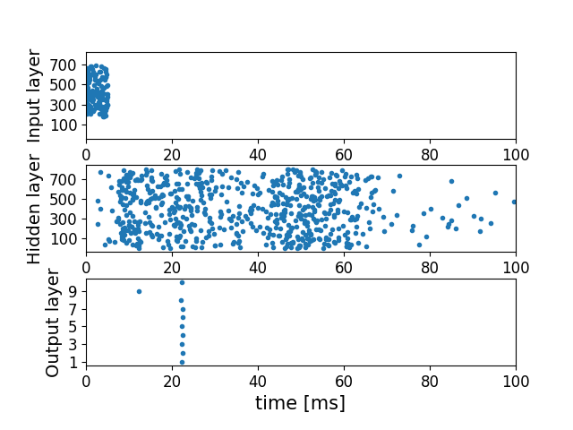
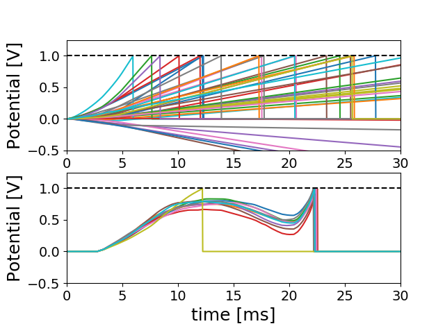
Fig. 5 shows the spike timing pattern (a raster plot) of a 2-layer SNN (784-800-10) after training for the input, the hidden, and output layers, from top to bottom, respectively. The horizontal axis represents the time in milliseconds and the vertical axis represents the index of neurons for each layer. These results show that the broad distribution of the spike timing in the hidden layer is such that a large portion of neurons in the hidden layer fire after the output neurons fire. In the output layer, the ninth output neuron fires the earliest, which corresponds to the correct label $(=8)$. Fig. 6 shows the time evolution of the membrane potential $v_{i}^{(l)}(t)$ of the neurons in each layer. The membrane potentials evolve as (1) such that their behavior can be expressed by a piecewise linear function. For the hidden layer, because the neurons receive no spikes from the input layer after 5 ms, their membrane potentials evolve linearly after the time 5 ms. For the output neurons, their membrane potential varies nonlinearly because they receive many spikes from the hidden layer. The membrane potential of the output neurons was observed to be suppressed by spikes from the hidden layer at approximately $10$ ms except that of the output neuron corresponding to the correct label. One neuron fired at approximately 12 ms and the others at approximately $t^{\text{Ref}}$. These results indicate that our proposed temporal penalty term is effective.

Figure 7: Raster plots for a 3-layer SNN (784-400-400-10). The hyperparameters are $\eta=200,t^{\text{(Ref)}}=60\text{ ms},\gamma=100,\text{ and }\epsilon=1$.

Figure 8: Time evolution of the membrane potentials of the neurons in the first layer (top), in the second layer (middle), and in the output layers (bottom), for a 3-layer SNN (784-400-400-10). The horizontal dashed lines represent the values of $V_{\text{th}}(=1)$. The hyperparameters are $\eta=1500,t^{\text{(Ref)}}=60\text{ ms},\gamma=100,\text{ and }\epsilon=1$.

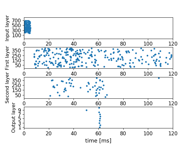
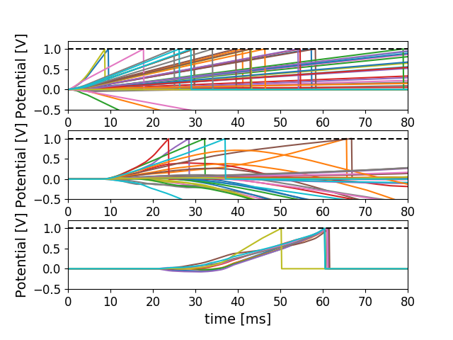
Similar but slightly different network dynamics is observed for 3-layer SNNs (784-400-400-10). Fig. 7 shows the raster plots of the spikes in the SNN. The distribution of spikes in the first hidden layer was broad, whereas that in the second hidden layer was relatively narrow. A large portion of neurons in the second hidden layer are observed not to have fired. This reduction in the number of firing neurons may imply that the neurons needed for information processing are selected for each data. Fig. 8 shows the time evolution of the membrane potential of the neurons in each layer. The results show that the membrane potentials of neurons in the second and output layers evolve nonlinearly, whereas those in the first layer evolve linearly after 5 ms.

Table 1: Performance comparisons on the MNIST dataset

Network	Coding	Accuracy
784-800-10 [56]	ANN	98.4 % [56]
784-800-800-10 [57]	ANN	98.8 % [57]
784-800-10 [32]	SNN (rate coding)	98.64 % [32]
784-300-300-10 [32]	SNN (rate coding)	98.77 % [32]
784-800-10 [37]	SNN (temporal coding)	97.55 % [37]
784-400-400-10 [37]	SNN (temporal coding)	97.14 % [37]
784-340-10 [38]	SNN (temporal coding)	97.96% [38]
784-500-10 (This work)	SNN (temporal coding)	97.83$\pm$0.07 %
784-800-10 (This work)	SNN (temporal coding)	98.04$\pm$0.05 %
784-300-300-10 (This work)	SNN (temporal coding)	97.73$\pm$0.08 %
784-400-400-10 (This work)	SNN (temporal coding)	97.90$\pm$0.12 %

Table 1 shows the results of the classification accuracy on the MNIST dataset. The standard errors ‘$\pm$’ for our results were obtained from 10 trials with different initial weights. The SNNs based on rate-coding [32] performed as good as ANNs[56, 57], whereas the SNNs based on temporal coding [37] performed slightly worse than ANNs. However, the improvements in our learning algorithm increased the performance of our algorithm compared with previous research [37], and the performance was slightly higher than [38]. Our best result is highlighted in bold in Table 1.

Figure 9: Time evolution of the membrane potentials of the neurons for 2-layer SNN (169-300-10) for $V_{\text{pulse}}$. (a) $V_{\text{pulse}}=128$, (b) $V_{\text{pulse}}=2$. In both (a) and (b), the upper and lower panels represent the first and the output layer, respectively. In the upper panel of (b), thee membrane potentials converge to some intermediate constants. The hyperparameters are $\eta=1500,t^{\text{(Ref)}}=21\text{ ms},\gamma=8,\text{ and }\epsilon=10$.

Figure 10: Classification accuracy on the shrunk MNIST dataset with various values of $V_{\text{pulse}}$ ($=2,4,8,\dots,128$) for 2-layer SNN (169-300-10). Each plot is the average of the results of five trials. The standard errors are smaller than the symbol size. The hyperparameters are $\eta=1500,t^{\text{(Ref)}}=21\text{ ms},\gamma=8,\text{ and }\epsilon=10$.

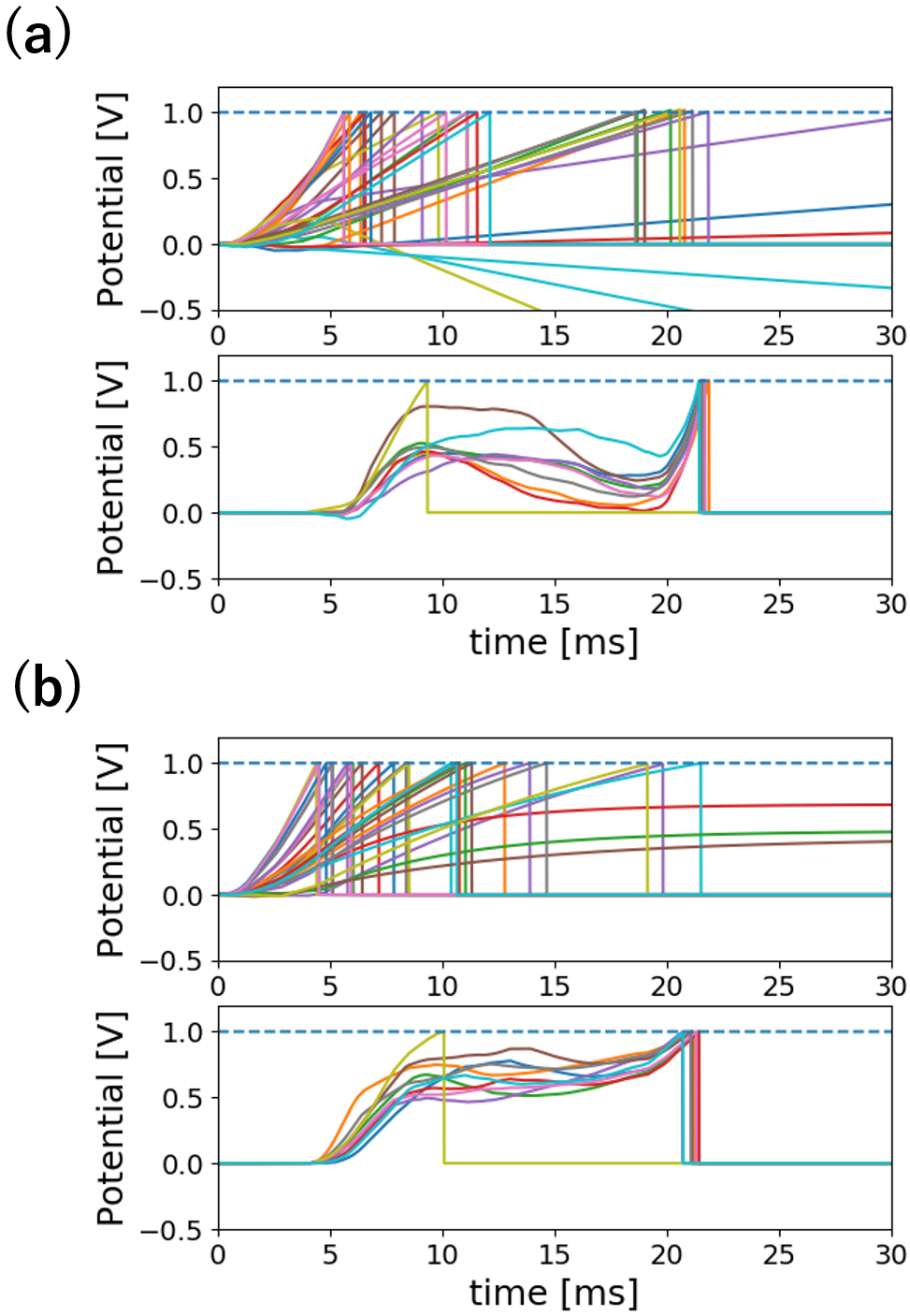
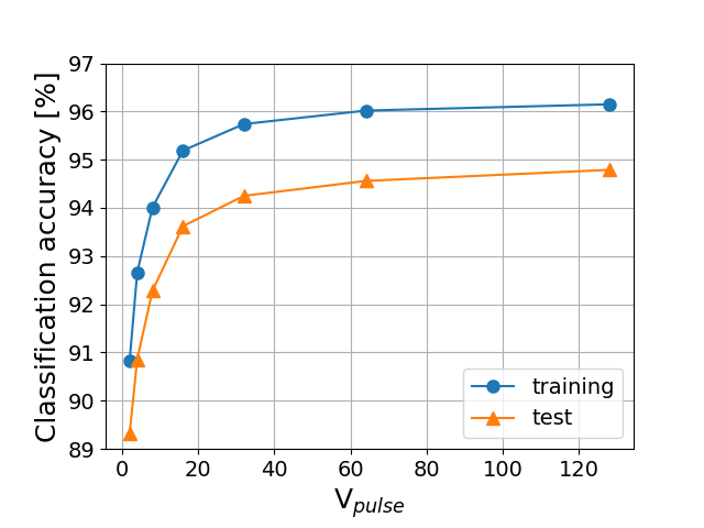
Next, we show the results of the learning performance when we replace the original neuron model (1) with the alternative neuron model (22). We again note that the model (22) is considered to be more energy efficient. To reduce the computational costs, we focused on a small-scale network (169-300-10) and used a shrunk version of the MNIST dataset. A shrunk MNIST image $\hat{\bm{x}}$ was obtained by convoluting a $4\times 4$ kernel of which the elements are all $1$ onto an original $28\times 28$ image $\bm{x}^{*}$ with a stride of 2. The $(i,j)$ pixel of the shrunk image $\hat{x}_{ij}$ is obtained by

$$\hat{x}_{ij} =\frac{1}{16}\sum_{k=0}^{3}\sum_{m=0}^{3}x_{2i+k-1~{}2j+m-1}^{*},~{}(i,j=1,2,\dots,13).$$ (33)

Then, we obtained spike patterns by using (26) with the flatted shrunk two-dimensional data $\hat{x}_{ij}$. In the experiment, we experienced difficulties in achieving learning convergence because of destructively large weight updates which had their origins in the temporal penalty term (9). We circumvented this difficulty by replacing the temporal penalty term (9) with

$$R(\bm{t}^{(M)}) :=\sum_{i=1}^{N^{(M)}}\left(t_{i}^{(M)}-t^{\text{(Ref)}}\right)^{3/2}$$ (34)

to soften the effect of its large weight updates when the timing of the output spike is far from $t^{\text{(Ref)}}$.

Fig. 9 shows the time evolution of the membrane potentials of the neurons for different values of $V_{\text{pulse}}$ ($=|V_{\text{pulse}}^{+}|=|V_{\text{pulse}}^{-}|$). When $V_{\text{pulse}}=128$ (Fig. 9(a)), the membrane potentials of the neurons in the hidden layer evolve linearly after 5 ms and those in the output layer evolve nonlinearly, which is similar to the case of Fig. 6. On the other hand, when $V_{\text{pulse}}=2$ (Fig. 9(b)), the membrane potentials of the neurons in the hidden evolve nonlinearly, which is caused by the term $v_{i}^{(l)}V_{\text{pulse}}^{ij}$ on the right-hand side of (22). Moreover, the membrane potentials of the neurons are stabilized at some intermediate value, because (22) has an equilibrium point with

$$v_{i}^{(l)}=\frac{\sum_{j\in\Gamma_{i}^{(l)}}w_{ij}^{(l)}}{\sum_{j\in\Gamma_{i}^{(l)}}w_{ij}^{(l)}V_{\text{pulse}}^{ij}}.$$ (35)

Fig. 10 shows the results of the classification accuracy for various values of $V_{\text{pulse}}$ ($=2,4,8,\dots,128$). As the value of $V_{\text{pulse}}$ decreases, the classification accuracy decreases monotonically. As shown in Fig. 9, there exists an equilibrium point in the membrane potential lower than $V_{\text{th}}$ when the value of $V_{\text{pulse}}$ is small, which may complicate the training.

5.2 Effects of manufacturing variations on learning performance

Figure 11: Classification accuracy of 2-layer SNN (784-500-10) with various variations of the firing threshold $\sigma_{V_{\text{th}}}^{\text{(train)}}$ at the training phase. The horizontal axis represents the value of $\sigma_{V_{\text{th}}}^{\text{(test)}}$ at the test phase. Each plotted point and error bar are the average and standard deviation of the results of ten trials, respectively. The hyperparameters are $\eta=1500,t^{\text{(Ref)}}=21\text{ ms},\gamma=100,\text{ and }\epsilon=1$.

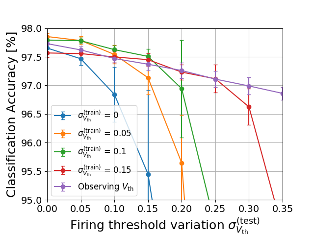
We present the results of the numerical simulation of the experiments described in 4.2. Fig. 11 shows the results of the classification accuracy for various values of the standard deviations of the firing threshold in the test phase $\sigma_{V_{\text{th}}}^{\text{(test)}}$. When no variation is assumed at the training phase ($\sigma_{V_{\text{th}}}^{\text{(train)}}=0$), the classification accuracy decreases conspicuously in the test phase as the standard deviation $\sigma_{V_{\text{th}}}^{\text{(test)}}$ increases. When variations are assumed in the training phase ($\sigma_{V_{\text{th}}}^{\text{(train)}}=0.05,~{}0.1,~{}0.15$) corresponding to case (i) in 4.2, the degradation of the classification accuracy can be suppressed to an extent. Especially, the suppression is effective when the variation in the test phase is almost the same as that assumed in the training phase ($\sigma_{V_{\text{th}}}^{\text{(train)}}\fallingdotseq\sigma_{V_{\text{th}}}^{\text{(test)}}$). When the values of all $V_{\text{th}}$ are known corresponding to case (ii) in 4.2, the degradation of the classification accuracy can be well suppressed.

Figure 12: Classification accuracy of 2-layer SNN (784-500-10) with various variations of spike delays $\sigma_{\tau}^{\text{(train)}}$ at the training phase. The horizontal axis represents the value of standard deviation of $\sigma_{\tau}^{\text{(test)}}$ at the test phase. Each plot and error bar are the average and standard deviation of the results of ten trials, respectively. The hyper parameters are $\eta=1500,t^{\text{(Ref)}}=21\text{ ms},\gamma=100,\text{ and }\epsilon=10$.

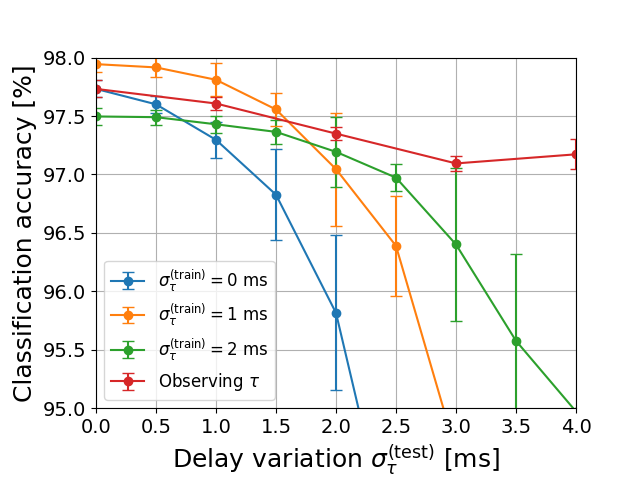
Next, the results of classification accuracy for various standard deviations of spike delays at the test phase $\sigma_{\tau}^{\text{(test)}}$ are shown in Fig. 12. As in the case of variations of firing threshold $V_{\text{th}}$ in Fig. 11, when no variation is assumed at the training phase ($\sigma_{\tau}^{\text{(train)}}=0$), the classification accuracy decreases as the standard deviation $\sigma_{\tau}^{\text{(test)}}$ at the test phase increases. While, when variations are assumed at the training phase ($\sigma_{\tau}^{\text{(train)}}=0,~{}1\text{ ms},~{}2\text{ ms}$) corresponding to case (ii) in 4.2, the degradation of classification accuracy can be suppressed to some extent. Especially, the suppression efficiently works when the variation at the test phase is almost the same as that assumed at the training phase ($\sigma_{\tau}^{\text{(train)}}\fallingdotseq\sigma_{\tau}^{\text{(test)}}$). When values of all $\tau^{(l)}_{ij}$ are known corresponding to case (ii) in 4.2, the degradation of classification accuracy can be well suppressed.

The series of numerical simulations shown above indicates that our proposed algorithm is robust against the device manufacturing variations. This fact paved a way to manufacturing VLSIs implementing the proposed algorithm.

6 Concluding remarks

In this study, we pursued the goal of achieving both high algorithmic performance and high energy efficiency by proposing a novel supervised learning algorithm for multilayer SNNs which can be implemented in VLSI circuits with analog resistive memory. We also proposed novel learning techniques such as adding a temporal penalty term to improve the learning performance.

Although the performance of the proposed algorithm on the MNIST dataset was slightly worse than SNNs based on rate coding and ANNs, the performance was confirmed to be as high as the state-of-the-art SNNs based on temporal coding. We showed that VLSI circuits can be designed with analog resistive memory in a simple and straightforward manner. We used numerical simulation to investigate the extent to which the learning performance depended on the circuit design. We also showed that the effects of manufacturing variations, which are unavoidable for real VLSI implementations, can be suppressed by estimating the magnitude of variations or by observing the exact values of these parameters. Therefore, we achieved our goal to a certain extent. The next step will be the fabrication of VLSI chips based on the circuits and algorithms proposed in this paper.

In this study, we focused on the development of energy-efficient algorithms for feedforward networks as a first step. Recently, it was shown that SNNs with recurrent connections can process time-series data with high performance [58, 59, 60]. For various applications of edge computing, the development of energy-efficient and hardware-friendly learning algorithms for SNN with recurrent connections is strongly anticipated. Thus, the development of these algorithms should be the next goal. Finally, we would like to remark that recent advances in biologically plausible and spike-based BP [61, 62, 63, 31, 64, 65] are foreseen to be beneficial to construct energy-efficient systems including the training process [66].

Appendix: Back propagation for case (22)

Figure 13: Schematic diagram of the time evolution of the membrane potential.

Here, we redefine the indices of the neurons to satisfy their indices to be sorted in the order of their spike time as

$$\hat{t}_{1}^{(l-1)}\leq\hat{t}_{2}^{(l-1)}\leq\dots\leq\hat{t}_{N^{(l-1)}}^{(l-1)}.$$ (36)

Then, we obtain the corresponding sorted weights

$$\hat{w}_{i1}^{(l)},\hat{w}_{i2}^{(l)},\dots,\hat{w}_{iN^{(l)}}^{(l)}.$$ (37)

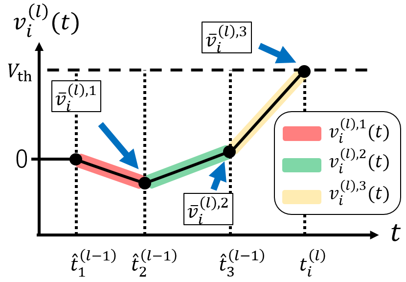
The time evolutions of the membrane potentials are piecewise such that they can be represented as the corresponding equations. For the $i$th neuron in the $l$th layer, from the moment when it receives the $k$th earliest spike to when it receives the $(k+1)$th earliest spike, the time evolution of its membrane potential $v_{i}^{(l),k}$ is described as

$$\frac{d}{dt}v_{i}^{(l),k} (t)=\sum_{j=1}^{k}\hat{w}_{ij}^{(l)}\left(1-v_{i}^{(l),k}V_{\text{pulse}}^{ij}\right),$$ (38)

for $$\hat{t}_{k}^{(l-1)}\leq t<\hat{t}_{k+1}^{(l-1)},~{}(k=1,2,\dots,N^{(l-1)}).$$ (39)

The terminal values of $v_{i}^{(l),k}$ are denoted by $\bar{v}_{i}^{(l),k}$ as follows:

$$\bar{v}_{i}^{(l),k} :=\begin{cases}v_{i}^{(l),k}\left(\hat{t}_{k+1}^{(l-1)}\right),\text{ for }k<G_{i}^{(l)}\\ v_{i}^{(l),G}\left(t_{i}^{(l)}\right),\text{ for }k=G_{i}^{(l)}\end{cases}$$ (40)

where $G_{i}^{(l)}$ represents the number of received spikes before the $i$th neuron fires, which can take different values for different neurons. Using the above definitions, we can obtain an analytical form of the membrane potential as follows:

$$\bar{v}_{i}^{(l),k} =\begin{cases}\frac{A_{i1}^{(l)}}{B_{i1}^{(l)}}-\frac{A_{i1}^{(l)}}{B_{i1}^{(l)}}\exp\left(-B_{i1}^{(l)}\Delta\hat{t}_{1}^{(l)}\right),\text{ for }k=1\\ \frac{A_{ik}^{(l)}}{B_{ik}^{(l)}}-\left(\frac{A_{ik}^{(l)}}{B_{ik}^{(l)}}-\bar{v}_{i}^{(l),k-1}\right)\exp\left(-B_{ik}^{(l)}\Delta\hat{t}_{k}^{(l)}\right),\\ ~{}~{}~{}~{}~{}~{}~{}~{}~{}~{}~{}~{}~{}~{}~{}~{}~{}~{}\text{ for }k=2,3,\dots,G_{i}^{(l)}\end{cases}$$ (41)

where

$$A_{ik}^{(l)} :=\sum_{j=1}^{k}\hat{w}_{ij}^{(l)}~{}~{}~{}B_{ik}^{(l)}:=\sum_{j=1}^{k}\hat{w}_{ij}^{(l)}V_{\text{pulse}}^{ij}$$ (42)

$$\Delta\hat{t}_{k}^{(l-1)} :=\begin{cases}\hat{t}_{k+1}^{(l-1)}-\hat{t}_{k}^{(l-1)},\text{ for }k=1,2,\dots,G_{i}^{(l)}-1\\ t_{i}^{(l)}-\hat{t}_{k}^{(l-1)},\text{ for }k=G_{i}^{(l)}.\end{cases}$$ (43)

Furthermore, the spike timing of the $i$th neuron in the $l$th layer is obtained as follows:

$$t_{i}^{(l)} =\begin{cases}\hat{t}_{G_{i}^{(l)}}^{(l-1)}-\frac{1}{B_{iG_{i}^{(l)}}^{(l)}}\ln\left(1-\frac{B_{iG_{i}^{(l)}}^{(l)}}{A_{iG_{i}^{(l)}}^{(l)}}V_{\text{th}}\right),\text{ for }G_{i}^{(l)}=1\\ \hat{t}_{G_{i}^{(l)}}^{(l-1)}-\frac{1}{B_{iG_{i}^{(l)}}^{(l)}}\ln\frac{\frac{A_{iG_{i}^{(l)}}^{(l)}}{B_{iG_{i}^{(l)}}^{(l)}}-V_{\text{th}}}{\left(\frac{A_{iG_{i}^{(l)}}^{(l)}}{B_{iG_{i}^{(l)}}^{(l)}}-\bar{v}_{i}^{(l),G_{i}^{(l)}-1}\right)},\text{ for }G_{i}^{(l)}>1.\end{cases}$$ (44)

Fig. 13 shows a schematic diagram of the time evolution of the membrane potential $v_{i}^{(l),k}(t)$ .

Similar to (10)–(15), the back propagation rule is then obtained by

$$\frac{\partial C}{\partial w_{jk}^{(l)}} =\frac{\partial\bar{v}_{j}^{(l),G_{i}^{(l)}}}{\partial w_{jk}^{(l)}}\delta_{j}^{(l)}$$ (45)

$$\delta_{s}^{(h)} =\begin{cases}\frac{\partial t_{s}^{(h)}}{\partial\bar{v}_{s}^{(h),G_{i}^{(l)}}}\sum_{i}^{N^{(h+1)}}\frac{\partial\bar{v}_{i}^{(h+1),G_{i}^{(l)}}}{\partial t_{s}^{(h)}}\delta_{i}^{(h+1)},\\ ~{}~{}~{}~{}~{}~{}~{}~{}~{}~{}~{}~{}~{}~{}~{}~{}~{}\text{ for }h=1,2,\dots,M-1\\ \frac{\partial t_{s}^{(M)}}{\partial\bar{v}_{s}^{(M),G_{i}^{(l)}}}\frac{\partial C}{\partial t_{s}^{(M)}},\text{ for }h=M\end{cases}$$ (46)

$$\frac{\partial C}{\partial t_{i}^{(M)}} =\kappa_{i}-S_{i}+\gamma\left(t_{i}^{(M)}-t^{\text{(Ref)}}\right).$$ (47)

Replacing $\{t_{i}^{(l)}\}$ and $\{w_{ij}^{(l)}\}$ with the sorted expressions $\{\hat{t}_{i}^{(l)}\}$ and $\{\hat{w}_{ij}^{(l)}\}$ given by (36) and (37), the derivatives on the right-hand sides of the above equations are obtained as follows:

for (45),

$$\frac{\partial\bar{v}_{i}^{(l),G_{i}^{(l)}}}{\partial\hat{w}_{ij}^{(l)}} =\begin{cases}\sum_{P=j}^{G_{i}^{(l)}}\frac{\partial\bar{v}_{i}^{(l),P}}{\partial\hat{w}_{ij}^{(l)}}\delta_{P}^{v_{i}^{(l)}},\text{ for }j=1,2,\dots,G_{i}^{(l)}\\ 0,\text{ for }j=G_{i}^{(l)}+1,G_{i}^{(l)}+2,\dots,N^{(l-1)}.\\ \end{cases}$$ (48)

In addition, for (46),

$$\delta_{j}^{v_{i}^{(l)}} =\begin{cases}\prod_{q=j}^{G_{i}^{(l)}-1}\frac{\partial\bar{v}_{i}^{(l),q+1}}{\partial\bar{v}_{i}^{(l),q}}=\frac{\partial\bar{v}_{i}^{(l),j+1}}{\partial\bar{v}_{i}^{(l),j}}\delta_{j+1}^{v_{i}^{(l)}}\\ ~{}~{}~{}~{}~{}~{}~{}~{}\text{ for }j=1,2,\dots,G_{i}^{(l)}-1\\ 1,\text{ for }j=G_{i}^{(l)}\\ \end{cases}$$ (49)

$$\frac{\partial\bar{v}_{i}^{(l),G_{i}^{(l)}}}{\partial\hat{t}_{j}^{(l-1)}} =\begin{cases}\frac{\partial\bar{v}_{i}^{(l),j}}{\partial\hat{t}_{j}^{(l-1)}}\delta_{j}^{v_{i}^{(l)}},\text{ for }j=1,2,\dots,G_{i}^{(l)}\\ 0,\text{ for }j=G_{i}^{(l)}+1,G_{i}^{(l)}+2,\dots,N^{(l-1)}\\ \end{cases}$$ (50)

$$\frac{\partial t_{i}^{(l)}}{\partial\bar{v}_{i}^{(l)}} =-\left(\frac{\partial\bar{v}_{i}^{(l),G_{i}^{(l)}}}{\partial t}\right)^{-1}$$

$$=\begin{cases}\frac{-1}{A_{iG_{i}^{(l)}}^{(l)}-B_{iG_{i}^{(l)}}^{(l)}V_{\text{th}}},\text{ when }G_{i}^{(l)}\geq 1\\ \frac{-1}{A_{iG_{i}^{(l)}}^{(l)}-B_{iG_{i}^{(l)}}^{(l)}V_{\text{th}}},\text{ when }G_{i}^{(l)}=0.\end{cases}$$ (51)

Note that the above equations take the value of $0$ when the $i$th neuron does not fire and (51) is derived from SpikeProp[36]. For the calculation of (48), we obtain the derivatives as follows:

$$\frac{\partial\bar{v}_{i}^{(l),k}}{\partial\hat{w}_{ij}^{(l)}} =\begin{cases}D_{ij}^{(l),k}\left(1-\exp\left(-B_{ik}^{(l)}\Delta\hat{t}_{k}^{(l-1)}\right)\right)\\ ~{}~{}+\left(\frac{A_{ik}^{(l)}}{B_{ik}^{(l)}}-\bar{v}_{i}^{(l),k-1}\right)\Delta\hat{t}_{k}^{(l-1)}V_{\text{pulse}}^{ij}\\ ~{}~{}~{}~{}\times\exp\left(-B_{ik}^{(l)}\Delta\hat{t}_{k}^{(l-1)}\right),\\ ~{}~{}~{}~{}~{}~{}~{}~{}~{}~{}~{}~{}~{}~{}~{}~{}~{}~{}~{}~{}~{}\text{ for }k=1,2,\dots,G_{i}^{(l)}\\ D_{ij}^{(l),k}\left(1-\exp\left(-B_{ik}^{(l)}\Delta\hat{t}_{k}^{(l-1)}\right)\right)\\ ~{}~{}+\frac{A_{ik}^{(l)}}{B_{ik}^{(l)}}\Delta\hat{t}_{k}^{(l-1)}V_{\text{pulse}}^{ij}\\ ~{}~{}~{}~{}\times\exp\left(-B_{ik}^{(l)}\Delta\hat{t}_{k}^{(l-1)}\right),\\ ~{}~{}~{}~{}~{}~{}~{}~{}~{}~{}~{}~{}~{}~{}~{}~{}~{}~{}~{}~{}~{}\text{ for }k=0\\ \end{cases}$$ (52)

where $D_{ij}^{(l),k}$ is defined as

$$D_{ij}^{(l),k}:=\frac{\partial}{\partial\hat{w}_{ij}^{(l)}}\left(\frac{A_{k}^{(l)}}{B_{k}^{(l)}}\right) =\frac{B_{k}^{(l)}-A_{k}^{(l)}V_{\text{pulse}}^{ij}}{B_{k}^{(l)2}},$$

$$~{}~{}~{}~{}~{}~{}\text{for }j=1,2,\dots,k.$$ (53)

Further, for (49),

$$\frac{\partial\bar{v}_{i}^{(l),k+1}}{\partial\bar{v}_{i}^{(l),k}} =\exp\left(-\Delta\hat{t}_{k+1}^{(l-1)}B_{k+1}^{(l)}\right),$$

$$~{}~{}~{}~{}~{}~{}\text{for }k=1,2,\dots,G_{i}^{(l)}-1.$$ (54)

Furthermore, (50) and (51) can be calculated with

$$\frac{\partial\bar{v}_{i}^{(l),k}}{\partial\hat{t}_{k}^{(l-1)}} =\begin{cases}\frac{\partial\bar{v}_{i}^{(l),k-1}}{\partial\hat{t}_{k}^{(l-1)}}\exp\left(-B_{ik}^{(l)}\Delta\hat{t}_{k}^{(l-1)}\right)\\ ~{}~{}-\left(A_{ik}^{(l)}-B_{ik}^{(l)}\bar{v}_{i}^{(l),k-1}\right)\\ ~{}~{}~{}~{}\times\exp\left(-B_{ik}^{(l)}\Delta\hat{t}_{k}^{(l-1)}\right),\\ ~{}~{}~{}~{}~{}~{}~{}~{}\text{ for }k=1,2,\dots,G\\ -A_{i0}^{(l)}\exp\left(-B_{i0}^{(l)}\Delta\hat{t}_{0}^{(l-1)}\right),\\ ~{}~{}~{}~{}~{}~{}~{}~{}\text{ for }k=0\end{cases}$$ (55)

$$\frac{\partial\bar{v}_{i}^{(l),k-1}}{\partial\hat{t}_{k}^{(l-1)}} =\begin{cases}\left(A_{ik-1}^{(l)}-B_{ik-1}^{(l)}\bar{v}_{i}^{(l),k-2}\right)\\ ~{}~{}\times\exp\left(-B_{ik-1}^{(l)}\Delta\hat{t}_{k-1}^{(l-1)}\right),\\ ~{}~{}~{}~{}~{}~{}~{}~{}~{}~{}~{}\text{ for }k=2,\dots,G\\ A_{i0}^{(l)}\exp\left(-B_{i0}^{(l)}\Delta\hat{t}_{0}^{(l-1)}\right),\\ ~{}~{}~{}~{}~{}~{}~{}~{}~{}~{}~{}\text{ for }k=1.\end{cases}$$ (56)

As described above, the BP for case (22) is obtained.

References

- [1] Alex Krizhevsky, Ilya Sutskever, and Geoffrey E Hinton. Imagenet classification with deep convolutional neural networks. In Advances in Neural Information Processing Systems, pp. 1097–1105. 2012.
- [2] Yann LeCun, Yoshua Bengio, and Geoffrey E. Hinton. Deep learning. Nature, Vol. 521, pp. 436–444, 2015.
- [3] S. Amari. A theory of adaptive pattern classifiers. IEEE Transactions on Electronic Computers, Vol. EC-16, No. 3, pp. 299–307, June 1967.
- [4] David E Rumelhart, Geoffrey E Hinton, Ronald J Williams, et al. Learning representations by back-propagating errors. Nature, Vol. 323, pp. 533–536, 1986.
- [5] Yann LeCun, Bernhard Boser, John S Denker, Donnie Henderson, Richard E Howard, Wayne Hubbard, and Lawrence D Jackel. Backpropagation applied to handwritten zip code recognition. Neural computation, Vol. 1, No. 4, pp. 541–551, 1989.
- [6] Kaiming He, Xiangyu Zhang, Shaoqing Ren, and Jian Sun. Deep residual learning for image recognition. In The IEEE Conference on Computer Vision and Pattern Recognition (CVPR), pp. 770–778, June 2016.
- [7] Gordon E Moore. Cramming more components onto integrated circuits. Electron. Mag, Vol. 38, No. 8, pp. 114–117, April 1965.
- [8] R. H. Dennard, F. H. Gaensslen, V. L. Rideout, E. Bassous, and A. R. LeBlanc. Design of ion-implanted MOSFET’s with very small physical dimensions. IEEE Journal of Solid-State Circuits, Vol. 9, No. 5, pp. 256–268, Oct 1974.
- [9] N. P. Jouppi, et al. In-datacenter performance analysis of a tensor processing unit. In 2017 ACM/IEEE 44th Annual International Symposium on Computer Architecture (ISCA), pp. 1–12, June 2017.
- [10] V. Sze, Y. Chen, T. Yang, and J. S. Emer. Efficient processing of deep neural networks: A tutorial and survey. Proceedings of the IEEE, Vol. 105, No. 12, pp. 2295–2329, Dec 2017.
- [11] W. Maass. To spike or not to spike: That is the question. Proceedings of the IEEE, Vol. 103, No. 12, pp. 2219–2224, Dec 2015.
- [12] Amirhossein Tavanaei, Masoud Ghodrati, Saeed Reza Kheradpisheh, Timothée Masquelier, and Anthony Maida. Deep learning in spiking neural networks. Neural Networks, Vol. 111, pp. 47–63, 2019.
- [13] Michael Pfeiffer and Thomas Pfeil. Deep learning with spiking neurons: Opportunities and challenges. Frontiers in Neuroscience, Vol. 12, No. 774, pp. 1–18, 2018.
- [14] Shih-Chii Liu, Tobi Delbruck, Giacomo Indiveri, Adrian Whatley, and Rodney Douglas. Event-based neuromorphic systems. John Wiley & Sons, 2015.
- [15] Ning Qiao, Hesham Mostafa, Federico Corradi, Marc Osswald, Fabio Stefanini, Dora Sumislawska, and Giacomo Indiveri. A reconfigurable on-line learning spiking neuromorphic processor comprising 256 neurons and 128k synapses. Frontiers in Neuroscience, Vol. 9, No. 141, pp. 1–17, 2015.
- [16] S. Moradi, N. Qiao, F. Stefanini, and G. Indiveri. A scalable multicore architecture with heterogeneous memory structures for dynamic neuromorphic asynchronous processors (dynaps). IEEE Transactions on Biomedical Circuits and Systems, Vol. 12, No. 1, pp. 106–122, Feb 2018.
- [17] J. Schemmel, D. Briiderle, A. Griibl, M. Hock, K. Meier, and S. Millner. A wafer-scale neuromorphic hardware system for large-scale neural modeling. In Proceedings of 2010 IEEE International Symposium on Circuits and Systems, pp. 1947–1950, May 2010.
- [18] S. Friedmann, J. Schemmel, A. Grübl, A. Hartel, M. Hock, and K. Meier. Demonstrating hybrid learning in a flexible neuromorphic hardware system. IEEE Transactions on Biomedical Circuits and Systems, Vol. 11, No. 1, pp. 128–142, Feb 2017.
- [19] Paul A. Merolla, et al. A million spiking-neuron integrated circuit with a scalable communication network and interface. Science, Vol. 345, No. 6197, pp. 668–673, 2014.
- [20] M. Davies, et al. Loihi: A neuromorphic manycore processor with on-chip learning. IEEE Micro, Vol. 38, No. 1, pp. 82–99, January 2018.
- [21] Catherine D. Schuman, et al. A survey of neuromorphic computing and neural networks in hardware. arXiv:1705.06963, May 2017.
- [22] Maxence Bouvier, et al. Spiking neural networks hardware implementations and challenges: A survey. J. Emerg. Technol. Comput. Syst., Vol. 15, No. 2, pp. 22:1–22:35, April 2019.
- [23] M. Horowitz. Computing’s energy problem (and what we can do about it). In 2014 IEEE International Solid-State Circuits Conference Digest of Technical Papers (ISSCC), pp. 10–14, Feb 2014.
- [24] N. Verma, H. Jia, H. Valavi, Y. Tang, M. Ozatay, L. Chen, B. Zhang, and P. Deaville. In-memory computing: Advances and prospects. IEEE Solid-State Circuits Magazine, Vol. 11, No. 3, pp. 43–55, Summer 2019.
- [25] Hsinyu Tsai, Stefano Ambrogio, Pritish Narayanan, Robert M Shelby, and Geoffrey W Burr. Recent progress in analog memory-based accelerators for deep learning. J. Phys. D: Appl. Phys., Vol. 51, No. 28, p. 283001, Jun 2018.
- [26] Daniele Ielmini and H-S Philip Wong. In-memory computing with resistive switching devices. Nature Electronics, Vol. 1, pp. 333–343, June 2018.
- [27] Qiangfei Xia and J Joshua Yang. Memristive crossbar arrays for brain-inspired computing. Nature materials, Vol. 18, No. 4, pp. 309–323, March 2019.
- [28] Emre Ozgur Neftci, Hesham Mostafa, and Friedemann Zenke. Surrogate gradient learning in spiking neural networks. arXiv:1901.09948, Jan 2019.
- [29] W. Maass. “Computing with Spiking Neurons,” in Pulsed Neural Networks, chapter 2, pp. 55–85. MIT Press, 1999.
- [30] Filip Ponulak and Andrzej KasiÅski. Supervised learning in spiking neural networks with ReSuMe: Sequence learning, classification, and spike shifting. Neural Computation, Vol. 22, No. 2, pp. 467–510, February 2010.
- [31] Emre O. Neftci, Charles Augustine, Somnath Paul, and Georgios Detorakis. Event-driven random back-propagation: Enabling neuromorphic deep learning machines. Frontiers in Neuroscience, Vol. 11, No. 324, pp. 1–16, June 2017.
- [32] Jun Haeng Lee, Tobi Delbruck, and Michael Pfeiffer. Training deep spiking neural networks using backpropagation. Frontiers in Neuroscience, Vol. 10, No. 508, pp. 1–12, November 2016.
- [33] Friedemann Zenke and Surya Ganguli. Superspike: Supervised learning in multilayer spiking neural networks. Neural computation, Vol. 30, No. 6, pp. 1514–1541, June 2018.
- [34] P. U. Diehl, D. Neil, J. Binas, M. Cook, S. Liu, and M. Pfeiffer. Fast-classifying, high-accuracy spiking deep networks through weight and threshold balancing. In 2015 International Joint Conference on Neural Networks (IJCNN), pp. 1–8, July 2015.
- [35] Steve K Esser, Rathinakumar Appuswamy, Paul Merolla, John V. Arthur, and Dharmendra S Modha. Backpropagation for energy-efficient neuromorphic computing. In Advances in Neural Information Processing Systems, pp. 1117–1125. 2015.
- [36] Sander M. Bohte, Joost N. Kok, and Han La Poutré. Error-backpropagation in temporally encoded networks of spiking neurons. Neurocomputing, Vol. 48, No. 1, pp. 17–37, October 2002.
- [37] H. Mostafa. Supervised learning based on temporal coding in spiking neural networks. IEEE Transactions on Neural Networks and Learning Systems, Vol. 29, No. 7, pp. 3227–3235, July 2018.
- [38] Iulia M Comsa, Krzysztof Potempa, Luca Versari, Thomas Fischbacher, Andrea Gesmundo, and Jyrki Alakuijala. Temporal coding in spiking neural networks with alpha synaptic function. arXiv:1907.13223, August 2019.
- [39] G. W. Burr, et al. Experimental demonstration and tolerancing of a large-scale neural network (165 000 synapses) using phase-change memory as the synaptic weight element. IEEE Transactions on Electron Devices, Vol. 62, No. 11, pp. 3498–3507, November 2015.
- [40] Shinhyun Choi, Jong Hoon Shin, Jihang Lee, Patrick Sheridan, and Wei D Lu. Experimental demonstration of feature extraction and dimensionality reduction using memristor networks. Nano letters, Vol. 17, No. 5, pp. 3113–3118, April 2017.
- [41] F Merrikh Bayat, M. Prezioso, B. Chakrabarti, H. Nili, I. Kataeva, and D. Strukov. Implementation of multilayer perceptron network with highly uniform passive memristive crossbar circuits. Nature communications, Vol. 9, No. 2331, June 2018.
- [42] Can Li, et al. Analogue signal and image processing with large memristor crossbars. Nature Electronics, Vol. 1, pp. 52–59, June 2018.
- [43] Fuxi Cai, et al. A fully integrated reprogrammable memristor–CMOS system for efficient multiply–accumulate operations. Nature Electronics, Vol. 2, pp. 290–299, July 2019.
- [44] Vishnu Ravinuthula, Vaibhav Garg, John G. Harris, and José A. B. Fortes. Time-mode circuits for analog computation. Int. J. Circ. Theor. Appl., Vol. 37, No. 5, pp. 631–659, 2009.
- [45] Ali Shafiee, et al. ISAAC: A convolutional neural network accelerator with in-situ analog arithmetic in crossbars. In Proceedings of the 43rd International Symposium on Computer Architecture, pp. 14–26, Piscataway, NJ, USA, 2016. IEEE Press.
- [46] M. J. Marinella, et al. Multiscale co-design analysis of energy, latency, area, and accuracy of a ReRAM analog neural training accelerator. IEEE Journal on Emerging and Selected Topics in Circuits and Systems, Vol. 8, No. 1, pp. 86–101, March 2018.
- [47] Stefano Ambrogio, et al. Equivalent-accuracy accelerated neural-network training using analogue memory. Nature, Vol. 558, pp. 60–67, June 2018.
- [48] Quan Wang, Hakaru Tamukoh, and Takashi Morie. Time-domain weighted-sum calculation for ultimately low power VLSI neural networks. In Neural Information Processing, Vol. 9947, pp. 240–247, September 2016.
- [49] Quan Wang, Hakaru Tamukoh, and T Morie. A time-domain analog weighted-sum calculation model for extremely low power VLSI implementation of multi-layer neural networks. arXiv:1810.06819, October 2018.
- [50] M. Bavandpour, M. R. Mahmoodi, and D. B. Strukov. Energy-efficient time-domain vector-by-matrix multiplier for neurocomputing and beyond. IEEE Transactions on Circuits and Systems II: Express Briefs, Vol. 66, No. 9, pp. 1512–1516, September 2019.
- [51] Masatoshi Yamaguchi, Goki Iwamoto, Hakaru Tamukoh, and Takashi Morie. An energy-efficient time-domain analog VLSI neural network processor based on a pulse-width modulation approach. arXiv:1902.07707, February 2019.
- [52] S. R. Nandakumar, Irem Boybat, Manuel Le Gallo, Evangelos Eleftheriou, Abu Sebastian, and Bipin Rajendran. Supervised learning in spiking neural networks with phase-change memory synapses. arXiv:1905.11929, May 2019.
- [53] Vinod Nair and Geoffrey E. Hinton. Rectified linear units improve restricted Boltzmann machines. In Proceedings of the 27th International Conference on International Conference on Machine Learning, pp. 807–814, USA, June 2010. Omnipress.
- [54] Y. LeCun, L. Bottou, Y. Bengio, and P. Haffner. Gradient-based learning applied to document recognition. Proceedings of the IEEE, Vol. 86, No. 11, pp. 2278–2324, November 1998.
- [55] D. Miyashita, S. Kousai, T. Suzuki, and J. Deguchi. A neuromorphic chip optimized for deep learning and CMOS technology with time-domain analog and digital mixed-signal processing. IEEE Journal of Solid-State Circuits, Vol. 52, No. 10, pp. 2679–2689, October 2017.
- [56] Nitish Srivastava, Geoffrey E. Hinton, Alex Krizhevsky, Ilya Sutskever, and Ruslan Salakhutdinov. Dropout: A simple way to prevent neural networks from overfitting. Journal of Machine Learning Research, Vol. 15, No. 1, pp. 1929–1958, January 2014.
- [57] Li Wan, Matthew Zeiler, Sixin Zhang, Yann Le Cun, and Rob Fergus. Regularization of neural networks using dropconnect. In Proceedings of the 30th International Conference on Machine Learning, Vol. 28, pp. 1058–1066, Jun 2013.
- [58] Wilten Nicola and Claudia Clopath. Supervised learning in spiking neural networks with force training. Nature communications, Vol. 8, No. 1, p. 2208, 2017.
- [59] Priyadarshini Panda and Narayan Srinivasa. Learning to recognize actions from limited training examples using a recurrent spiking neural model. Frontiers in Neuroscience, Vol. 12, No. 126, pp. 1–14, 2018.
- [60] Guillaume Bellec, Darjan Salaj, Anand Subramoney, Robert Legenstein, and Wolfgang Maass. Long short-term memory and learning-to-learn in networks of spiking neurons. In Advances in Neural Information Processing Systems, pp. 787–797. 2018.
- [61] Timothy P Lillicrap, Daniel Cownden, Douglas B Tweed, and Colin J Akerman. Random synaptic feedback weights support error backpropagation for deep learning. Nature communications, Vol. 7, No. 1, p. 13276, November 2016.
- [62] Arild Nøkland. Direct feedback alignment provides learning in deep neural networks. In Advances in Neural Information Processing Systems, pp. 1037–1045. 2016.
- [63] Jordan Guerguiev, Timothy P Lillicrap, and Blake A Richards. Towards deep learning with segregated dendrites. eLife, Vol. 6, pp. 1–37, 2017.
- [64] Guillaume Bellec, Franz Scherr, Elias Hajek, Darjan Salaj, Robert Legenstein, and Wolfgang Maass. Biologically inspired alternatives to backpropagation through time for learning in recurrent neural nets. arXiv:1901.09049, January 2019.
- [65] James C.R. Whittington and Rafal Bogacz. Theories of error back-propagation in the brain. Trends in Cognitive Sciences, Vol. 23, No. 3, pp. 235–250, 2019.
- [66] J. Park, J. Lee, and D. Jeon. A 65nm 236.5nj/classification neuromorphic processor with 7.5% energy overhead on-chip learning using direct spike-only feedback. In 2019 IEEE International Solid-State Circuits Conference, pp. 140–142, Feb 2019.