Enhancing CFD predictions in shape design problems by model and parameter space reduction

Abstract

In this work we present an advanced computational pipeline for the approximation and prediction of the lift coefficient of a parametrized airfoil profile. The non-intrusive reduced order method is based on dynamic mode decomposition (DMD) and it is coupled with dynamic active subspaces (DyAS) to enhance the future state prediction of the target function and reduce the parameter space dimensionality. The pipeline is based on high-fidelity simulations carried out by the application of finite volume method for turbulent flows, and automatic mesh morphing through radial basis functions interpolation technique. The proposed pipeline is able to save $1/3$ of the overall computational resources thanks to the application of DMD. Moreover exploiting DyAS and performing the regression on a lower dimensional space results in the reduction of the relative error in the approximation of the time-varying lift coefficient by a factor $2$ with respect to using only the DMD.

1 Introduction

Reduced order modeling (ROM) is nowadays a quite popular and consolidated technique, applied to several fields of engineering and computational science thanks to the remarkable computational gain granted for the solution of the governing equations. The ROM goal is in fact that of reducing the dimension of the studied system without altering some important properties of the original problem. This typically results in more efficient, time saving computations. Among other fields, ROM methods are frequently and successfully applied to problems governed by parametric partial differential equations (PDEs), for which many solutions of the same PDE in correspondence with different parameters are required. This paradigm is for example encountered in the context of parametric optimal control problems, uncertainty quantification, and shape optimization.

Model reduction for PDEs has been historically obtained in different ways. In some cases, very successful reduced models have been obtained at the level of the governing equations, based on physical considerations. This is for instance the case of the potential flow theory in the fluid dynamics field. In other cases, the reduction can be introduced at the discretization level, as is the case, for instance, for the Boundary Element Method used in structural analysis, fluid mechanics, electro-magnetism and acoustics studies. In the case in which parametric PDEs are considered, a possible approach to obtain efficient reduced order models is to sample the solution manifold by creating a solutions database corresponding to different parameters, using a high-dimensional discretization, then combine the latter to identify the intrinsic lower dimension of the problem. For parametric reduced order models see [24, 44, 46], while for a more applications oriented overview we suggest [54, 47, 48].

For parametric time-dependent problems, a proper orthogonal decomposition approach can be applied to reduce the dimensionality of the system, as in [20, 27]. In this work we propose a novel data-driven approach for parametric dynamical systems, combining dynamic mode decomposition (DMD) with active subspaces (AS) property. These two relatively new methodologies provide a simplification of the dynamical system, and an analysis of the input parameter space of a given target function, respectively. Exploiting AS property we are able to obtain an estimation of the importance of the parameters of such function, as well as a reduction in the number of parameters. Moreover the methods are equation-free, being based only on input/output couples and do not make assumptions on the underlying governing equations.

We define a generic scalar output $v(\bm{\mu},t)\in\mathbb{R}$ that depends both on time $t$ and on the parameters of the model $\bm{\mu}\in\mathbb{D}\subset\mathbb{R}^{k}$, with $k$ denoting the dimension of the parameter space. We denote the state of the parametric system at time $t$ with $v_{t}(\bm{\mu})\in\mathbb{R}$. The solution manifold in time is approximated using the DMD in order to obtain an approximation of the linear map $A$ defined as:

$$v_{t+1}(\bm{\mu})=A(v_{t}(\bm{\mu})).$$ (1)

It is easy to note that using (1) we have the possibility to forecast a generic future state of the parametric system.

To numerically compute the linear operator $A$, we need to sample the parameter space $\mathbb{D}$, and for each time store the quantity of interest for each parametric configuration. Formally, considering a set of parameter samples with dimension $Ns$, the discrete vector referring to the system state at time $t$ results:

$$\mathbf{v}_{t}=\begin{bmatrix}v_{t}({\bm{\mu}_{1}})&\dotsc&v_{t}({\bm{\mu}_{Ns}})\end{bmatrix}^{T}\in\mathbb{R}^{Ns}.$$ (2)

Collecting several time states $\mathbf{v}_{i}(\bm{\mu})$ for $i=1,\dotsc,m$, we compute the operator $\mathbf{A}$ with a best-fit approach such that $\mathbf{v}_{t+1}\approx\mathbf{A}\mathbf{v}_{t}$. Once computed the future prevision, we are able to exploit the relation between the input parameters $\bm{\mu}_{i}$ and the related outputs $v_{\text{future}}(\bm{\mu}_{i})$ to approximate the output for any new parameter. In this work we use a Gaussian Process Regression (GPR) [60, 23], but any regression or interpolation method can be used. We underline that the chosen regression model has to be fitted for any forecasted time we want to analyse.

The high dimensionality in the parameter space may incur on the inability to solve many-query problems with sufficiently high fidelity, thus causing a decrease in the accuracy of the solution approximation. For this reason we couple the regression with the AS property in order to perform a sensitivity analysis of function $v_{t}(\bm{\mu})$. AS indeed is able to provide an approximation $g$ of a scalar function $f$, where the input parameters of $g$ are a linear combination of the original parameters of $f$. The coefficients of such combination give information about the importance of the original parameters. In this work, we use this information to reduce the dimension of the parameter space — in which we build the regression — by not considering the parameters whose AS coefficients are smaller than a certain threshold, that is they are almost zero.

The developed methodology is tested on an aeronautics application given by the flow past an airfoil profile. As output of interest we considered the lift coefficient and the parameters vector $\bm{\mu}$ describes geometrical transformations according to the morphing technique proposed in [25]. The fluid dynamics problem is described using the incompressible Navier–Stokes equations with turbulence modeling. These are discretized using a finite volume approximation. The deformed meshes corresponding to different input parameters are automatically obtained exploiting a Radial Basis Function (RBF) mesh morphing technique.

This work is structured as follows: in section 2 we present the general parametric problem over which we apply the proposed numerical pipeline, providing some information about the geometrical deformation. In section 3 and section 4 we present the DMD and AS methods, respectively, while in section 5 we show the numerical setting of the problem and the results obtained. Finally in section 6 we propose some final remarks and highlight possible future developments.

2 The parametric problem

Let be given the unsteady incompressible Navier-Stokes equations described in an Eulerian framework on a parametrized space-time domain $Q(\bm{\mu})=\Omega(\bm{\mu})\times[0,T]\subset\mathbb{R}^{d}\times\mathbb{R}^{+},\textrm{ }d=2,3$ with the vectorial velocity field $\bm{u}:Q(\bm{\mu})\to\mathbb{R}^{d}$, and the scalar pressure field $p:Q(\bm{\mu})\to\mathbb{R}$ such that:

$$\begin{cases}\bm{u_{t}}+\bm{\nabla}\cdot(\bm{u}\otimes\bm{u})-\bm{\nabla}\cdot 2\nu\bm{\nabla^{s}}\bm{u}=-\bm{\nabla}p&\mbox{ in }Q(\bm{\mu}),\\ \bm{\nabla}\cdot\bm{u}=\bm{0}&\mbox{ in }Q(\bm{\mu}),\\ \bm{u}(t,x)=\bm{f}(\bm{x})&\mbox{ on }\Gamma_{\text{in}}\times[0,T],\\ \bm{u}(t,x)=\bm{0}&\mbox{ on }\Gamma_{0}(\bm{\mu})\times[0,T],\\ (\nu\nabla\bm{u}-p\bm{I})\bm{n}=\bm{0}&\mbox{ on }\Gamma_{\text{out}}\times[0,T],\\ \bm{u}(0,\bm{x})=\bm{k}(\bm{x})&\mbox{ in }Q(\bm{\mu})_{0},\\ \end{cases}$$ (3)

holds. Here, $\Gamma=\Gamma_{\text{in}}\cup\Gamma_{0}\cup\Gamma_{\text{out}}$ is the boundary of $\Omega(\bm{\mu})$ and it is composed by three different parts $\Gamma_{\text{in}}$, $\Gamma_{\text{out}}$ and $\Gamma_{0}(\bm{\mu})$ that indicate, respectively, inlet boundary, outlet boundary, and physical walls. The term $\bm{f}(\bm{x})$ depicts the stationary non-homogeneous boundary condition, whereas $\bm{k}(\bm{x})$ denotes the initial condition for the velocity at $t=0$. Shape changes are applied to the domain $\Omega$, and in particular to its boundary $\Gamma_{0}(\bm{\mu})$ corresponding to the airfoil wall. Such shape modifications are associated to numerical parameters contained in the vector $\bm{\mu}\in\mathbb{R}^{k}$ which, in the numerical examples shown in this work has dimension $k=10$. As said, the only portion of the domain boundary subject to shape parametrization is the physical wall of the airfoil $\Gamma_{0}(\bm{\mu})$, which in the undeformed configuration corresponds to the 4-digits, NACA 4412 wing profile [3, 29]. To alter such geometry, we adopt the shape parametrization and morphing technique proposed in [25], where $k$ shape functions are added to the airfoil profiles. Let $y_{u}$, and $y_{l}$ be the upper and lower ordinates of a NACA profile, respectively. We express the deformation of such coordinates as

$$y_{u} =\overline{y_{u}}+\sum_{i=1}^{5}c_{i}r_{i},$$ (4)

$$y_{l} =\overline{y_{l}}-\sum_{i=1}^{5}d_{i}r_{i},$$ (5)

where the bar denotes the reference undeformed state, which is the NACA 4412 profile.

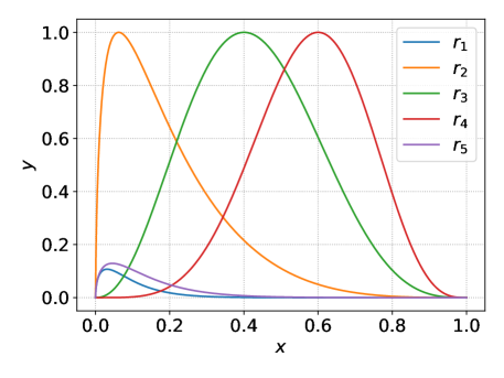
The parameters $\bm{\mu}\in\mathbb{D}\subset\mathbb{R}^{10}$ are the weights coefficients, $c_{i}$ and $d_{i}$, associated with the shape functions $r_{i}$. The range of each parameter will be specified in section 5. The explicit formulation of the shape functions can be found in [25], we report them in Figure 1.

Figure 1: Airfoil shape functions with respect to the profile abscissa. The leading edge corresponds to $x=0$.

After the reference profile is deformed, we also apply the same morphing to the mesh coordinates by using a radial basis functions (RBF) interpolation method [9, 42, 41]. With this approach the movement $\bm{s}$ of all the points which do not belong to the moving boundaries is approximated by an interpolatory radial basis function:

$$\bm{s}(\bm{x})=\sum_{i=1}^{N_{b}}\beta_{i}\xi(||\bm{x}-\bm{x}_{b_{i}}||)+q(\bm{x}),$$ (6)

where $\bm{x}_{b_{i}}$ are the coordinates of points for which we know the boundary displacements, for this particular case the points located on the wing surface. $N_{b}$ is the number of control points on the boundary, $\xi$ is a given basis function, $q(\bm{x})$ is a polynomial. The coefficients $\beta_{i}$ and the polynomial $q(\bm{x})$ are obtained by the imposition of interpolation conditions

$$\bm{s}(\bm{x}_{b_{i}})=\bm{d}_{b_{i}},$$ (7)

where $\bm{d}_{b_{i}}$ is the displacement value at the boundary points and by the additional requirement:

$$\sum_{i=1}^{N_{b}}\beta_{i}q(\bm{x}_{b_{i}})=0.$$ (8)

In the present case, we select basis functions for which it is possible to use linear polynomials $q(\bm{x})$. For more informations concerning the selection of the order of polynomials see [5]. Finally the values of the coefficients $\beta_{i}$ and the coefficients $\delta_{i}$ of the linear polynomials $q$ can be obtained by solving the linear problem:

$$\begin{bmatrix}\bm{d}_{b}\\ 0\end{bmatrix}=\begin{bmatrix}\bm{M}_{b,b}&P_{b}\\ P_{b}^{T}&0\end{bmatrix}\begin{bmatrix}\bm{\beta}\\ \bm{\delta}\end{bmatrix},$$ (9)

where $\bm{M}_{b,b}\in\mathbb{R}^{N_{b}\times N_{b}}$ is a matrix containing the evaluation of the basis functions $\xi_{b_{i}b_{j}}=\xi(\lVert\bm{x}_{b_{i}}-\bm{x}_{b_{j}}\rVert)$, and $\bm{P}_{b}\in\mathbb{R}^{N_{b}\times(d+1)}$ is a matrix where $d$ is the spatial dimension. Each row of this matrix, that contains the coordinates of the boundary points, is given by $\mbox{row}_{i}(\bm{P}_{b})=\begin{bmatrix}1&\bm{x_{b_{i}}}\end{bmatrix}$. Once the system of (9) is solved one can obtain the displacement of all the internal points using the RBF interpolation:

$$\bm{d}_{\text{in}_{i}}=\bm{s}(\bm{x}_{\text{in}_{i}}),$$ (10)

where $\bm{x}_{\text{in}_{i}}$ are the coordinates of the internal grid points. The computation of the displacement of the grid points entails the resolution of a dense system of equations that has dimension $N_{b}+d+1$. Usually, the number of boundary points $N_{b}$ is much smaller than the number of grid points $N_{h}$.

3 Dynamical systems approximation by dynamic mode decomposition

Dynamic mode decomposition (DMD) is an emerging reduced order method proposed by Schmid in [49] for the analysis of dynamical systems. Approximating the linear infinite-dimensional Koopman operator [32], DMD decomposes the original system into few main features, the so called DMD modes, that evolve linearly in time, even if the original system has nonlinear behaviour. This means that, other than individuating recurrent patterns in the evolution of the system, DMD provides a real-time midcast/forecast of the output of interest. An important advantage of such method is the complete data-driven nature: the algorithm relies only on the system output, without the necessity of any information regarding the model or equations used.

Dynamic mode decomposition has been successfully employed in naval hull shape optimization pipelines [15], for online real-time acquisitions in a wind tunnel experiment [63], and in meteorology [6], among others. We also mention the higher order DMD extension [36, 37].

In the following paragraph, we provide just an algorithmic overview of the method. For an exhaustive explanation of DMD, its applicability, and possible extensions, we suggest [33, 8].

We define the linear operator $\bm{\mathbf{A}}$ such that

$$\bm{\mathbf{x}}_{k+1}=\bm{\mathbf{A}}\bm{\mathbf{x}}_{k},$$ (11)

where $\bm{\mathbf{x}}_{k+1}\in\mathbb{R}^{N}$ and $\bm{\mathbf{x}}_{k}\in\mathbb{R}^{N}$ are the vectors containing the system outputs at two sequential instants. Thus, the operator $\bm{\mathbf{A}}:\mathbb{R}^{N}\to\mathbb{R}^{N}$ expresses the dynamics of the system. In order to construct it using only data, we need to collect $m\leq N+1$ equispaced in time outputs $\bm{\mathbf{x}}_{i}$ for $i=1,\dotsc,m$ — from now on called snapshots — then arrange them in two matrices: $\mathbf{X}=\begin{bmatrix}\mathbf{x}_{1}&\dotsc&\mathbf{x}_{m-1}\end{bmatrix}$ and $\mathbf{Y}=\begin{bmatrix}\mathbf{x}_{2}&\dotsc&\mathbf{x}_{m}\end{bmatrix}$. Since the corresponding columns in $\bm{\mathbf{X}}$ and $\bm{\mathbf{Y}}$ are sequential snapshots, we are able to use (11) to represent the relationship between $\mathbf{X}$ and $\mathbf{Y}$, such that $\bm{\mathbf{Y}}=\bm{\mathbf{A}}\bm{\mathbf{X}}$. We can find such operator by using the relation $\bm{\mathbf{A}}=\bm{\mathbf{Y}}\bm{\mathbf{X}}^{\dagger}$, where ^† refers to the Moore-Penrose pseudo-inverse. We exploit the singular value decomposition to compute such pseudo-inverse, due to its computational efficiency and accuracy, as in the following:

$$\bm{\mathbf{X}}=\bm{\mathbf{U}}\bm{\mathbf{\Sigma}}\bm{\mathbf{V}}^{*},$$ (12)

where the matrix $\bm{\mathbf{U}}\in\mathbb{R}^{N\times(m-1)}$ contains the orthogonal left-singular vectors. We can then project the operator onto the space spanned by the left-singular vectors to get the reduced operator $\bm{\mathbf{\tilde{A}}}$. It is possible to note that the reduced operator does not require the construction of the high-dimensional one:

$$\bm{\mathbf{\tilde{A}}}=\bm{\mathbf{U}}^{*}\bm{\mathbf{A}}\bm{\mathbf{U}}=\bm{\mathbf{U}}^{*}\bm{\mathbf{Y}}\bm{\mathbf{X}}^{\dagger}\bm{\mathbf{U}}=\bm{\mathbf{U}}^{*}\bm{\mathbf{Y}}\bm{\mathbf{V}}\bm{\mathbf{\Sigma}}^{-1}\bm{\mathbf{U}}^{*}\bm{\mathbf{U}}=\bm{\mathbf{U}}^{*}\bm{\mathbf{Y}}\bm{\mathbf{V}}\bm{\mathbf{\Sigma}}^{-1}.$$ (13)

We can now reconstruct the eigenvectors and eigenvalues of the matrix $\mathbf{A}$ thanks to the eigendecomposition of $\mathbf{\tilde{A}}$ as $\mathbf{\tilde{A}}\mathbf{W}=\mathbf{W}\bm{\Lambda}$. In particular each nonzero eigenvalue $\lambda$ in $\bm{\Lambda}$ is a DMD eigenvalue. The corresponding DMD eigenvectors, the so called exact modes [57], can be retrieved by the eigenvectors of $\mathbf{\tilde{A}}$ as $\bm{\mathbf{\Phi}}=\mathbf{Y}\mathbf{V}\bm{\mathbf{\Sigma}}^{-1}\mathbf{W}$, where different scalings are possible. We underline that each pair $(\phi,\lambda)$ computed as above is an eigenpair of $\mathbf{A}$ (please refer to the proof of Theorem 1 in [57]). Thus, being $\bm{\mathbf{A}}=\bm{\mathbf{\Phi}}\bm{\mathbf{\Lambda}}\bm{\mathbf{\Phi}}^{\dagger}$, we can approximate the evolution of the system $\bm{\mathbf{x}}_{k+1}=\bm{\mathbf{\Phi}}\bm{\mathbf{\Lambda}}\bm{\mathbf{\Phi}}^{\dagger}\bm{\mathbf{x}}_{k}$. Moreover, it is easy to demonstrate that the approximation of a generic future snapshots can be computed as:

$$\bm{\mathbf{x}}_{k+j}=\bm{\mathbf{\Phi}}\bm{\mathbf{\Lambda}}^{j}\bm{\mathbf{\Phi}}^{\dagger}\bm{\mathbf{x}}_{k}.$$ (14)

In this work we compute the DMD modes of the matrix composed by the value of the time-varying lift coefficient for a set of given geometrical parameters. Then we can predict the future state of the coefficient and, using a regression method, approximate the target function at untried new parameters. All the DMD computation have been carried out by the Python package PyDMD [16].

4 Global sensitivity analysis through Active Subspaces

Active subspaces [10] have been successfully employed in many engineering fields [12, 13]. Among other we mention applications in shape optimization [40, 21], combustion simulations [31], in naval engineering [55], and in optimization procedures coupled with genetic algorithm [18]. For multifidelity dimension reduction with AS see [34], for multivariate extension of AS we mention [62], while for a coupling with deep neural networks see [56]. A kernel-based extension of AS for multivariate functions we be found in [45].

Active subspaces have also been proven as a useful tool to enhance model order reduction techniques such as proper orthogonal decomposition (POD) with interpolation for structural and fluid dynamics problems [17], and POD-Galerkin methods for a parametric study of carotid artery stenosis [53].

Here we briefly introduce the active subspaces property for functions not depending on time, for the details and estimates regarding the method we refer to [10]. For the actual computations to find AS we used the open source Python package ATHENA - Advanced Techniques for High dimensional parameter spaces to Enhance Numerical Analysis [2], derived in part from the Python Active subspaces Utility Library [14].

Let $\bm{\mu}\in\mathbb{R}^{k}$ the parameters of our problem, $f$ be a parametric scalar function of interest $f(\bm{\mu}):\mathbb{R}^{k}\to\mathbb{R}$, and $\rho:\mathbb{R}^{k}\to\mathbb{R}^{+}$ a probability density function representing uncertainty in the input parameters. Active subspaces are a property of the pair $(f,\rho)$. They are defined as the leading eigenspaces of the second moment matrix of the target function’s gradient and constitutes a global sensitivity index more general than coordinate-aligned derivative-based ones [62].

The second moment matrix of the gradients $\mathbf{C}$, also called uncentered covariance matrix of the gradients of $f$ with respect to the input parameters, is defined as

$$\mathbf{C}=\mathbb{E}\,[\nabla_{\bm{\mu}}f\,\nabla_{\bm{\mu}}f^{T}]=\int(\nabla_{\bm{\mu}}f)(\nabla_{\bm{\mu}}f)^{T}\rho\,d\bm{\mu},$$ (15)

where $\mathbb{E}[\cdot]$ is the expected value, and $\nabla_{\bm{\mu}}f\equiv\nabla f({\bm{\mu}})\in\mathbb{R}^{k}$. $\mathbf{C}$ is symmetric thus it admits a real eigenvalue decomposition that reads:

$$\mathbf{C}=\mathbf{W}\Lambda\mathbf{W}^{T},$$ (16)

where $\mathbf{W}$ indicates the orthogonal matrix containing the eigenvectors of $\mathbf{C}$ as columns, and $\Lambda$ is a diagonal matrix composed by the non-negative eigenvalues arranged in descending order. We can decompose the two matrices as follows

$$\Lambda=\begin{bmatrix}\Lambda_{1}&\\ &\Lambda_{2}\end{bmatrix},\qquad\mathbf{W}=\left[\mathbf{W}_{1}\quad\mathbf{W}_{2}\right],\qquad\mathbf{W}_{1}\in\mathbb{R}^{k\times M},$$ (17)

where $M<k$ has to be properly selected by identifying a spectral gap. In particular, we define the active subspace of dimension $M$ as the principal eigenspace corresponding to the eigenvalues prior to the gap. Then we can map the full parameters to the reduced ones through $\mathbf{W}_{1}$. We define the active variable as $\bm{\mu}_{M}=\mathbf{W}_{1}^{T}\bm{\mu}\in\mathbb{R}^{M}$, and the inactive variable as $\bm{\eta}=\mathbf{W}_{2}^{T}\bm{\mu}\in\mathbb{R}^{k-M}$. In practice the matrix $\mathbf{C}$ is constructed with a Monte Carlo procedure.

AS stipulates that the directional derivatives in directions belonging to the kernel of $\mathbf{W}_{1}^{T}$ are significantly smaller that those belonging to the range of the same matrix. Moreover this assumptions are made in expectation rather then in absolute sense [61].

Since in this way we are considering a linear combinations of the input parameters, we can associate the eigenvectors elements to the weights of such combinations, thus providing a sensitivity of each parameter. We underline that if a weight is almost zero, that means $f$ does not vary along that direction on average.

We can use the active variable to build a ridge function $g$ [38] to approximate the function of interest, that is

$$f(\bm{\mu})\approx g(\mathbf{W}_{1}^{T}\bm{\mu})=g(\bm{\mu}_{M}).$$ (18)

In this work we want to study the behaviour of a target function $f(\bm{\mu},t):\mathbb{R}^{k}\times\mathbb{R}^{+}\to\mathbb{R}$ that depends on the parameters $\bm{\mu}$ and on time $t$ as well. This results in extending the active subspaces property to dynamical systems, that means having to deal with time-dependent uncentered covariance matrix $\mathbf{C}(t)$, and corresponding eigenvectors $w_{i}(t)$. Efforts in this direction has been done in [11] for a lithium ion battery model, in [39] for long term model of HIV infection dynamics, and more recently an application of dynamic mode decomposition and sparse identification to approximate one-dimensional active subspaces in [4]. In these works they refer to dynamic active subspaces (DyAS) as the time evolution of the active subspaces of a time-dependent quantity of interest.

DyAS are useful to assess the importance of each input parameter at given times and to study how the weights associated to the inputs evolve. In the following we are going to compute the AS for a set of equispaced times $t_{i}$. If some of the parameters are almost zero in the entire time window we can safely ignore them in the construction of the Gaussian process regression.

5 Computational pipeline

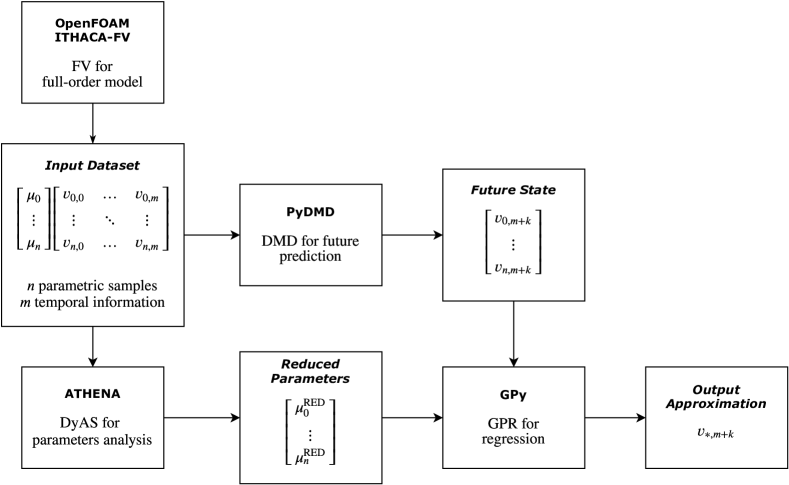
In the present section we will discuss the numerical experiments carried out to test the DyAS analysis and present the results obtained. As reported in section 2, each high fidelity simulation is based on a parametric fluid dynamic model governed by the Reynolds Averaged Navier–Stokes (RANS) equations. Thus, a number of flow simulations have been carried out selecting different samples in the parametric space to test the performance — in terms of lift coefficient — of different airfoil shapes. The simulations made use of both the RANS solver provided in the OpenFOAM [58] finite volumes library, and of the DMD acceleration methodology described in section 3. Once the lift coefficients output were available for all the samples tested in the input parameters space, the DyAS analysis was applied to assess possible parameter redundancy. The elimination of the redundant parameters detected in the DyAS analysis allowed for the generation of a surface response model based on a lower dimensional space, which has been finally tested against the original RANS model accelerated through DMD, and against the surface response model based on the original input parameter space. Figure 2 graphically summarizes the proposed pipeline, clarifying how the methods (and the software) are integrated together, while the following sections will further detail each part of the computational pipeline just outlined.

Figure 2: Flowchart representing the proposed computational pipeline.

5.1 Parametric shape deformation

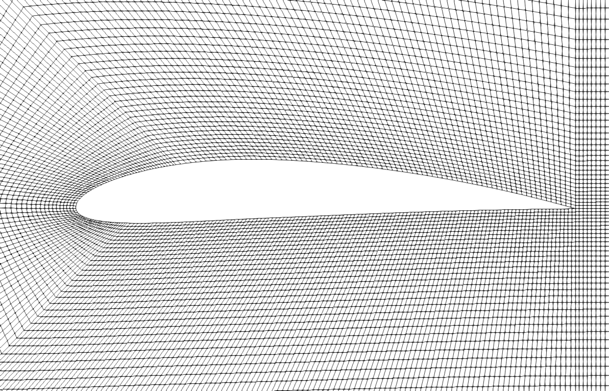
The fluid dynamics problem is resolved using the finite volume method. The wing is immersed in a rectangular domain according to Figure 3. The reference mesh counts $46500$ hexahedral cells and is constructed using the blockMesh utility of the OpenFOAM library. Figure 3 depicts a detail of the grid in proximity of the wing. The meshes in the deformed configuration have been obtained starting from the reference configuration using a radial basis function smoothing algorithm similar to the one implemented in [7]. A single deformation corresponds to a sample $\bm{\mu}$ in the parameter space $\mathbb{D}:=[0,0.03]^{10}\subset\mathbb{R}^{10}$. Therefore all the deformed meshes share the same number of cells and the same mesh topology. In particular Wendland [59] second order kernel functions with radius $r_{\text{RBF}}=0.1~{}$\mathrm{m}$$ have been used. The control points of the RBF procedure have been placed on each mesh boundary point located onto the wing surface. Since the outer boundary points are fixed we decided to neglect them from the RBF computation using a smoothing function defined in such a way that the RBF contribution reduces to zero after a certain distance from a focal point [30]. Particularly, the focal point has been placed in the geometric center of the airfoil chord segment and the distance from the focal point after which the RBF contribution is neglected is set to $r_{\text{out}}=7~{}$\mathrm{m}$$. In Figure 4 we depict the envelope of all the tested configurations, and the flow velocity streamlines for a particular sample in the parameter space. A uniform and constant velocity equal to $\bm{u}_{\text{in}}=1~{}$\mathrm{m}$/$\mathrm{s}$$ is set at the inlet boundary, while the constant value of the kinematic viscosity is set to $\nu=2\mathrm{e}{-5}~{}$\mathrm{m}^{2}$/$\mathrm{s}$$. This configuration, considering a chord length $D=1~{}$\mathrm{m}$$, corresponds to Reynolds number $\mathrm{Re}=50000$. As well known, a flow characterized by Reynolds number of such magnitude requires turbulence modeling to be numerically simulated with reasonable computational effort. In the present work, turbulence has been modeled using a RANS approach with a Spalart-Allmaras turbulence model [50]. The pressure velocity coupling is resolved in a segregated manner making use of the PIMPLE algorithm which merges the PISO [28] and the SIMPLE [43] algorithm. The time step used to advance the simulation in time is set constant and equal to $\Delta t=1\mathrm{e}-3~{}$\mathrm{s}$$. The convective terms have been discretized using a second-order upwinding scheme, while the diffusion terms are discretized using a linear approximation scheme with non-orthogonal correction. The time discretization is resolved using a second order backward differentiation formula. The simulation is advanced in time until the flow has reached stationary behavior. For the present problem, setting a total simulation time $T_{s}=30~{}$\mathrm{s}$$ is sufficient to reach a solution which is reasonably close to the steady state one. In order to check the consistency of the numerical results, the stationary lift coefficient computed for the reference configuration, which corresponds to a standard NACA $4412$ profile with a $0^{\circ}$ angle of attack, has been compared with data from literature [1]. The computed lift coefficient for such setting is equal to $C_{L}=0.355$ and the available reference value varies between $C_{L}=0.1804$ and $C_{L}=0.3708$ depending on the value of $N_{\mbox{crit}}$ (which is used to model the turbulence of the fluid or roughness of the airfoil). Therefore, our numerical results are in line with available data in existing literature.

Figure 3: Sketch of the computational domain used to solve the fluid dynamics problem in its reference configuration. The left picture reports a schematic view on the domain with the main geometrical dimensions. The right plot reports a zoom on the mesh in the proximity of the wing.

Figure 4: The left picture reports in light blue the envelope of all the tested configurations used during the training stage. The right picture depicts the flow velocity streamlines for one particular sample inside the training set $\bm{\mu}=[0.0071;0.0229;0.0015;0.0015;0.0087;0.0107;0.0033;0.0130;0.0247;0.0280]$.

5.2 Parameter space reduction

The present section will discuss the application of DyAS to the problem of the two dimensional turbulent flow simulation past airfoil sections with parameterized shape. Such a fluid dynamic problem is relevant in several engineering fields, as it is encountered in a number of industrial applications, ranging from aircraft and automotive design, to turbo machinery and propeller modeling. We must here point out that in this work, the DMD method is used for faster evaluation of the parameterized airfoils lift towards a steady state regime solution. We remark that, since DMD is designed for time evolutionary problems, the same procedure can be used in the same fashion, to speed up convergence to periodic regime solutions [35]. Indeed, recent work on hydroacoustic computations based on LES suggested that DMD modal decomposition can successfully be employed in the reconstruction of complex and turbulent flow fields [19] provided that the snapshots used are enough to characterize all the relevant time and space frequencies in the flow. In addition, we observed that complex full order flows characterized by richer spectra require a higher amount of modes to obtain accurate flow fields reconstruction. Thus, our experience suggests that the ROM instruments used in this work are indeed effective when employed with more complex physics. For such reason, given our experience, we infer that the design pipeline here presented can also be used to study the unsteady dynamics of bubbles and vortices past the airfoil. Obviously one requirement of such type of problems would be a suitable FOM model able to capture transition phenomena occurring in the stall region. For example, we believe that the underlying high fidelity URANS solver would not be appropriate and that a transition to a LES approach would be required. For projection-based ROMs in a turbulent setting see [27, 51, 26].

A few plots describing the DyAS results for the lift coefficient output are presented in Figure 6, 7, 8, and 9. The plots in the figures are aimed at representing the evolution of the active subspace effectiveness and composition over the time dependent flow simulations. More specifically, the left diagram in each figure plots the lift coefficient at each sample point tested, as a function of the first active variable obtained through a linear combination of the sample point coordinates in the parameter space, that is $f(\bm{\mu},t)$ against $\mathbf{W}_{1}^{T}\bm{\mu}$.

Figure 5: The temporal evolution of the lift coefficient from $1~{}$\mathrm{s}$$ to $30~{}$\mathrm{s}$$ for $9$ different parameters, together with the mean (dashed). The angle of attack is fixed for all the airfoil profiles and it is equal to $0^{\circ}$.

Presenting the components of the first eigenvector of the uncentered covariance matrix, the right plot in each figure indicates the weights used in such linear combination to obtain the first active variable. In summary, the right diagram in each Figure suggests the impact of each of the original parameters on the first active variable, while the left diagram is an indicator of how well a one dimensional active subspace is able to represent the input to output relationship. Following the evolution of these two indicators it is possible, at each time instant, to assess how effective the one dimensional parameter dimension reduction is, and what is the sensitivity of the reduced lift coefficient output to variations of the original parameters.

Figure 6: On the left the sufficiency summary plot for the lift coefficient at time $t=6.0$ seconds. On the right the first eigenvector components at the corresponding parameters.

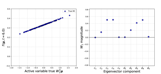
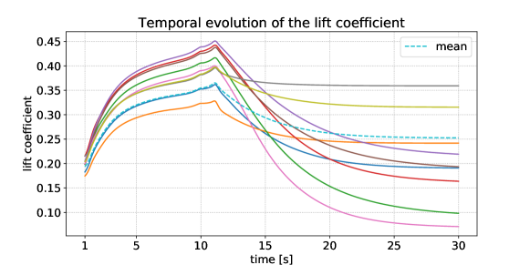
The plots in  Figure 6, 7, 8, and 9 show the results of the DyAS at the fixed time instants $t=6~{}$\mathrm{s}$,10~{}$\mathrm{s}$,14~{}$\mathrm{s}$,18~{}$\mathrm{s}$$, respectively. We here remark that, given the aforementioned considerations about the solution build up in the first 12 seconds of the simulations, the solutions at $t=6~{}$\mathrm{s}$$ and $t=10~{}$\mathrm{s}$$ are not entirely relevant by a physical perspective. Yet, presenting such cases is still helpful in illustrating how the DyAS evolve over time and can be used to evaluate the system behavior and the output sensitivities with respect to the input parameters. For completeness in Figure 5 we depicted the temporal evolution of $9$ different morphed airfoils, and the mean among all the airfoils. A first look at the right plots for each time steps, suggests that the contribution of the parameters corresponding to the bump shape functions $r_{1}$, and $r_{5}$, for both the top and the bottom part of the airfoil profile are almost negligible. This means the lift coefficient is almost insensitive to variations of these 4 parameters. Alternatively, it can be said that the output function is on average almost flat along directions corresponding to the axes corresponding to parameters $c_{1}$, $c_{5}$, $d_{1}$, and $d_{5}$.

Figure 7: On the left the sufficiency summary plot for the lift coefficient at time $t=10.0$ seconds. On the right the first eigenvector components at the corresponding parameters.

Figure 8: On the left the sufficiency summary plot for the lift coefficient at time $t=14.0$ seconds. On the right the first eigenvector components at the corresponding parameters.

Figure 9: On the left the sufficiency summary plot for the lift coefficient at time $t=18.0$ seconds. On the right the first eigenvector components at the corresponding parameters.

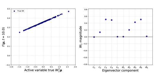
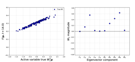
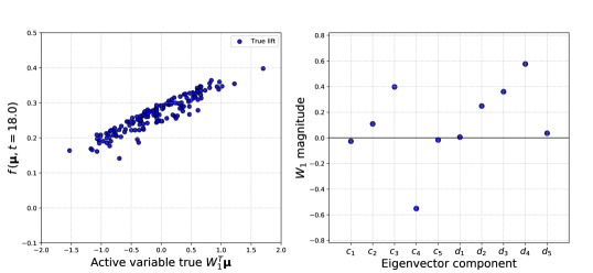
Figure 6 and 7 present the characterization of the one dimensional active subspace at time $t=6~{}$\mathrm{s}$$ and $t=10~{}$\mathrm{s}$$, respectively. We can clearly see that the lift coefficient is perfectly approximated along the identified direction, and such direction (the eigenvector elements) is almost the same at $t=6~{}$\mathrm{s}$$ and $t=10~{}$\mathrm{s}$$. This should not completely surprise as both time instants are included in an initial acceleration phase during which the air coming from the inflow boundary is reaching the airfoil. Given the domain arrangement described in Figure 3, the flow velocity around the impulsively started airfoil leading edge is expected to reach the inflow value at time $t=10~{}$\mathrm{s}$$. For such reason, we will focus the description on the plots for $t=10~{}$\mathrm{s}$$, although the considerations can be immediately reproduced for previous time steps. The left plot in Figure 7 suggests that at this meaningful instant, the first active subspace represents the input to output relationship with remarkably good accuracy. In fact, only a single output value corresponds to each active variable value. In other words, when plotted against the first variable, the output appears like a curve — a line in the present case. A look at the right diagram suggests that the shape parameters having the most impact on the lift generated by the airfoil are $c_{3}$, $c_{4}$, $d_{3}$ and $d_{4}$, which are the ones associated to shape functions with peaks located around the middle of the airfoil chord. The positive values of the eigenvector components associated to $c_{3}$, $c_{4}$, $d_{3}$ and $d_{4}$, along with the positive slope of the curve in the left plot in Figure 7 suggest that, at this particular time instant, higher values of lift can be obtained by increasing the airfoil thickness in the mid-chord region.

Similar considerations can be drawn from Figure 8, which refers the the DyAS analysis carried out at $t=14~{}$\mathrm{s}$$. Here, the points in the left diagram do not completely cluster on top of a single valued curve as was the case for the previous time step considered. Compared to what has been observed at $t=10~{}$\mathrm{s}$$, the data clearly indicate that at $t=14~{}$\mathrm{s}$$ an input to output relationship obtained using only a one dimensional active subspace will lead to less accurate lift coefficient predictions. Yet, the points in the plot are still all located within a rather narrow band surrounding a regression line having positive slope. Thus, all the considerations on the lift coefficient sensitivity with respect to variations of the shape parameters that can be inferred from the right plot, will still hold at least by a qualitative standpoint. Here, the eigenvector components suggest that the most influential parameters on the lift coefficient are $c_{3}$, $d_{3}$ and $d_{4}$, while $c_{2}$ and $d_{2}$ affect the output in lesser but not negligible fashion. Compared to the previous case the importance of coefficient $c_{4}$ on the output is significantly reduced. We recall that $c_{4}$ is associated with increased $y$ coordinates of the airfoil suction side past the mid-chord region. Thus, we might infer that in the acceleration phase higher lift values are obtained not only increasing the front thickness, but also lowering the camber line in the region past mid-chord.

Figure 9 shows the results of the DyAS analysis at $t=18~{}$\mathrm{s}$$, when the flow approaches the final regime solution. Following the trend observed for $t=14~{}$\mathrm{s}$$, the left plot in the figure indicates that a one dimensional active subspace is not completely able to represent the input to output relationship in a satisfactory fashion. With respect to the previous plots, the output values are here located in an even wider band around a regression line with positive slope. Again, on one hand this increasingly blurred picture suggests that higher dimensional active subspaces are required to reproduce the steady state solution with sufficient accuracy; on the other hand, the diagram still suggests a quite definite trend in the output, which can be exploited for qualitative considerations. Quite interestingly, at the present time step the eigenvector component corresponding to the $c_{4}$ coefficient has negative sign. Given the positive slope of the input to output relationship in the left plot of Figure 9, this implies that increases in the airfoil ordinates on the top side in the region past the mid-chord result in lift loss. Thus, this seems to suggest that an airfoil with a higher camber line curvature, combined with a thicker leading edge region might result in increased lift. This should not surprise, as a similar kind of airfoil would result in a higher downwash due to the increased camber line curvature, yet being able to avoid stall by means of a thicker and rounder leading edge. Thus, the DyAS analysis at different time steps shows that as the impulsively started airfoil moves from an acceleration phase to a steady state regime solution, the shape modifications leading to increased lift transit from a purely symmetric increase of the thickness in the mid-chord region, to a non-symmetric modification of the camber line united with a symmetric leading edge thickness increase, respectively. Such behavior is indicated by the sign of $c_{4}$ coefficient in the eigenvector characterizing the one dimensional active subspace, which is likely detecting that at steady state, regime solution, airfoils with higher camber line curvature and thicker leading edges produced higher downwash.

We underline that the eigenvector components of all the time instants presented corresponding to the coefficients $c_{1}$, $c_{5}$, $d_{1}$, and $d_{5}$ are almost zero. This means that on average the lift coefficient is almost flat along these directions. We are going to exploit this fact by freezing these parameters and constructing a GPR on a reduced parameter space.

5.3 GPR approximation and prediction of the lift coefficient

Figure 10: Sensitivity analysis of the dimension of the training set for the DMD (left) and for the response surface using GPR (right). For the DMD, we use 70 samples (of the parametric space) evolving in time in $[12,20]~{}$\mathrm{s}$$ and we measure the mean relative error at time $30~{}$\mathrm{s}$$ varying the sampling frequency; for the GPR, we build the response surface using up to 70 sampling lift coefficients at time $20~{}$\mathrm{s}$$ and computing the mean relative error over the test dataset composed by 100 test deformations.

The previous analysis pointed out the presence of several input parameters with minimal average influence on the target function. Making use of such consideration we construct a response surface which only depends on the remaining parameters. Both for the full parameter space and the reduced one, we use a Gaussian process regression with a RBF kernel implemented in the open source Python package GPy [22]. We then compare the performance of the two regression strategies by computing the relative error over a test data set composed by 100 samples. The error is computed as the Euclidean norm of the difference between the exact and the approximated solution over the norm of the exact solution. The training set is composed by the same 70 samples, in 10 dimensions for the GPR over the original parameter spaces, and in 6 dimensions for the reduced one. Up to $t=20~{}$\mathrm{s}$$ the training is done using the high-fidelity simulations.

Figure 11: The relative error of the approximated outputs at different times. The relative error is computed on 100 test samples, using the high-fidelity lift coefficient to train the regression for $t\leq 20~{}$\mathrm{s}$$, while for $t>20~{}$\mathrm{s}$$ the DMD forecasted states are used for the training.

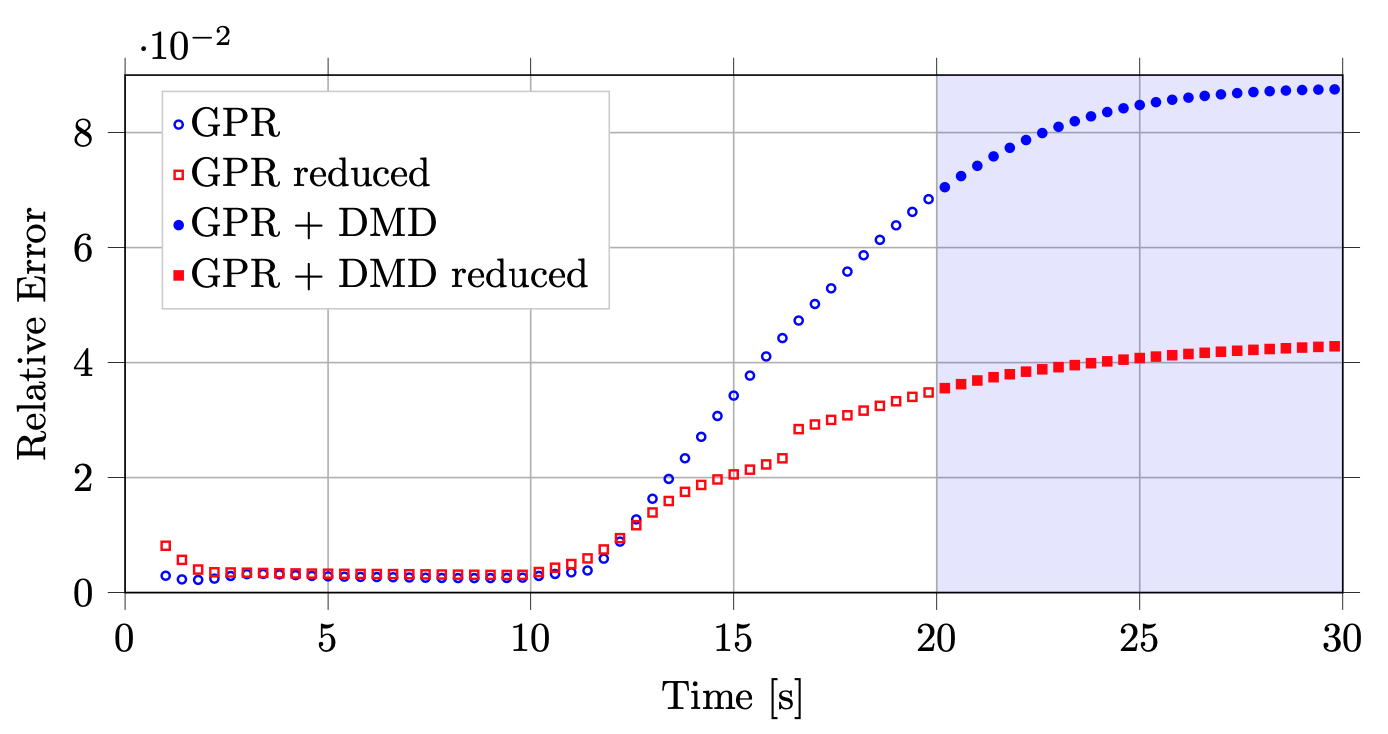
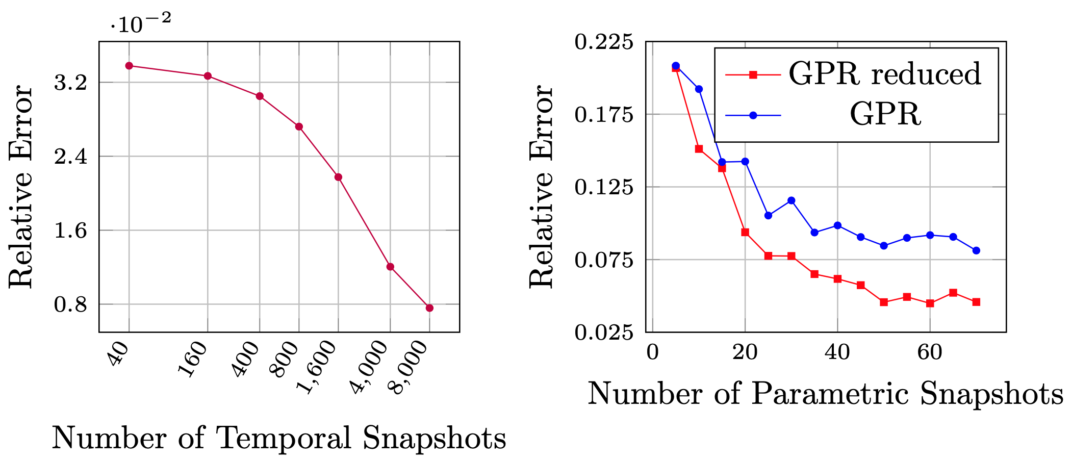
To speed up the convergence to the regime state ($t=30~{}$\mathrm{s}$$) we applied the DMD to get the future-state prediction of the lift. In particular, due to the initial propagation of the boundary conditions, for all the 70 training deformations we use the trend of lift coefficients within the temporal interval $[12,20]~{}$\mathrm{s}$$ to fit the DMD model, that means $8000$ temporal information ($\Delta t=0.001~{}$\mathrm{s}$$). Since we used 10 POD modes — selected using the energetic criterion — for the projection of the DMD operator, our low-rank operator results of dimension $10$. Despite in this case the dimensional reduction is not huge, this approach allows to predict the future state in a very fast fashion. In the high-fidelity model, we need in fact $1508$ CPU seconds (on average) to simulate $1$ second of the physical model, instead using DMD we can approximate a future state in less than $0.1$ CPU seconds. In practices, this means that, to reach the regime state with the standard approach, the simulation lasts $1508~{}$\mathrm{s}$\times 30\approx 45000~{}$\mathrm{s}$$, while with the DMD we have $1508~{}$\mathrm{s}$\times 20+0.1~{}$\mathrm{s}$\approx 30000~{}$\mathrm{s}$$, guaranteeing to save $\textstyle\frac{1}{3}$ of the overall computational load. All the simulations, both at the FOM and at the ROM level have been run serially on an Intel Xeon E5-2640, 2.50GHz CPU. We highlight that this is only a part of the computational saving of the pipeline that we are proposing and is related to the training stage. The DMD allows in fact for $1/3$ reduction of the simulation time required to the FOM as the remaining time is simulated by an approximated model. On the other side, once the reduced order model has been constructed, exploiting the combination of the Gaussian Process approximation and the DMD, it is possible to test new geometries in real time, with a negligible computational cost. Regarding the accuracy, we present in Figure 10 a sensitivity analysis on the number of training snapshots, varying the temporal sampling period $\Delta t_{\text{DMD}}$ from $1\mathrm{e}-3~{}$\mathrm{s}$$ to $0.2~{}$\mathrm{s}$$ and measuring the error on the predicted state at $t=30~{}$\mathrm{s}$$. Similarly, we propose an analysis on the GPR accuracy: using a varying number of lift coefficients at $t=20~{}$\mathrm{s}$$, we build the response surface and measure the error for untried parameters, both in the full dimensional space and in the reduced one. In Figure 11 we compare the two GPR performance at each of the time steps analyzed in the simulations. Until $12~{}$\mathrm{s}$$, the regressions behave in a very similar fashion, while from $15~{}$\mathrm{s}$$ the accuracy gain obtained by distributing the 70 samples in a lower dimensional space becomes significant. The error gap between the 6 and 10 dimensional response surface in fact, consistently increases from $0.016$ at $15~{}$\mathrm{s}$$ to $0.045$ at steady state. This corresponds to a decrement of the error by a factor $2$.

The proposed method achieves better results because it exploits the DyAS to discard the directions of the input parameter space along which the target function does not vary.

6 Conclusions and perspectives

We presented a computational pipeline to improve the approximation of the time-varying lift coefficient of a parametrized NACA airfoil. The pipeline comprises automatic mesh deformation through RBF interpolation, high-fidelity simulation with finite volume method of turbulent flow past the airfoil, global sensitivity analysis exploiting AS, and future state prediction via DMD reduced order method. This resulted in more accurate Gaussian process regression of the lift coefficient even if in a reduced parameter space. Despite the turbulent nature of the flow, the selected testcase does not show highly nonlinear phonemena — e.g. stall, reattachment — that usually occur in several fluid dynamics problems. The proposed framework can be extendend to address also more complex applications, provided that a suitable number of snapshots is given to characterize the parameter space and frequencies required by the DMD training. Of course such more demanding training requirements would likely result in reduced ROMs speed up and would require case-specific treatments.

After the creation of the high-fidelity solutions database the application of AS highlighted a possible reduction of the parameter space due to negligible contributions of $4$ different parameters. We exploit this reduction to construct a GPR over a smaller parameter space, thus improving its performance. Since the training of the regression model is done over $6$ dimension instead of $10$, given the same high-fidelity database dimension, the GPR is able to better approximate the solution manifold. This results in better lift coefficient predictions for new untried parameters. We also applied DMD to have future-state prediction of the target function up to $30$ seconds and proved that the effective gain of the new GPR is preserved also for any time after the $20$ seconds simulated with FV. In particular from $13$ seconds the actual gain is significant, at $15$ seconds we have an increased performance by a factor $2$ in the relative error, which means that performing the regression in the reduced parameter space produces a relative error equal to $0.02$, instead of $0.036$. Evolving in the future the error drop increases up to $0.045$ at regime ($0.042$ instead of $0.087$, keeping the factor $2$).

This computational pipeline can be seen as a parametric dynamic mode decomposition for some extent. Moreover, the sensitivity analysis has a negligible computational cost with respect to the creation of the offline high-fidelity database.

Future developments can be the study of adaptive sampling strategies exploiting a generic $n$-dimensional active subspace, and the coupling of different model order reduction methods. Another possible extension of the presented method regards the possibility to apply the framework to a flow field — e.g. pressure, velocity — rather than to a scalar output. It would be interesting to use this non-intrusive setting as a preprocessing tool to reduce the number of simulations required to build a reduced basis space which is later used in an intrusive manner [52]. We think this new computational pipeline can be of much interest in the context of shape optimization and dynamical systems.

References

- [1] Airfoil Tools. Airfoil database search. http://www.airfoiltools.com/, 2020.
- [2] ATHENA: Advanced Techniques for High dimensional parameter spaces to Enhance Numerical Analysis. https://github.com/mathLab/ATHENA, 2020.
- [3] I. H. Abbott and A. E. Von Doenhoff. Theory of wing sections: including a summary of airfoil data. Courier Corporation, 2012.
- [4] I. P. Aguiar. Dynamic Active Subspaces: a Data-Driven Approach to Computing Time-Dependent Active Subspaces in Dynamical Systems. Master’s thesis, University of Colorado Boulder, 2018.
- [5] A. Beckert and H. Wendland. Multivariate interpolation for fluid-structure-interaction problems using radial basis functions. Aerospace Science and Technology, 5(2):125–134, feb 2001.
- [6] D. A. Bistrian and I. M. Navon. An improved algorithm for the shallow water equations model reduction: Dynamic Mode Decomposition vs POD. International Journal for Numerical Methods in Fluids, 78(9):552–580, 2015.
- [7] F. M. Bos, B. W. van Oudheusden, and H. Bijl. Radial basis function based mesh deformation applied to simulation of flow around flapping wings. Computers & Fluids, 79:167–177, June 2013.
- [8] S. L. Brunton and J. N. Kutz. Data-driven science and engineering: Machine learning, dynamical systems, and control. Cambridge University Press, 2019.
- [9] M. D. Buhmann. Radial basis functions: theory and implementations, volume 12. Cambridge University Press, 2003.
- [10] P. G. Constantine. Active subspaces: Emerging ideas for dimension reduction in parameter studies, volume 2. SIAM, 2015.
- [11] P. G. Constantine and A. Doostan. Time-dependent global sensitivity analysis with active subspaces for a lithium ion battery model. Statistical Analysis and Data Mining: The ASA Data Science Journal, 10(5):243–262, 2017.
- [12] P. G. Constantine, E. Dow, and Q. Wang. Active subspace methods in theory and practice: applications to kriging surfaces. SIAM Journal on Scientific Computing, 36(4):A1500–A1524, 2014.
- [13] P. G. Constantine, M. Emory, J. Larsson, and G. Iaccarino. Exploiting active subspaces to quantify uncertainty in the numerical simulation of the HyShot II scramjet. Journal of Computational Physics, 302:1–20, 2015.
- [14] P. G. Constantine, R. Howard, A. G. Salinger, Z. Grey, P. Diaz, and L. Fletcher. Python Active-subspaces Utility Library. J. Open Source Software, 1(5):79, 2016.
- [15] N. Demo, M. Tezzele, G. Gustin, G. Lavini, and G. Rozza. Shape optimization by means of proper orthogonal decomposition and dynamic mode decomposition. In Technology and Science for the Ships of the Future: Proceedings of NAV 2018: 19th International Conference on Ship & Maritime Research, pages 212–219. IOS Press, 2018.
- [16] N. Demo, M. Tezzele, and G. Rozza. PyDMD: Python Dynamic Mode Decomposition. The Journal of Open Source Software, 3(22):530, 2018.
- [17] N. Demo, M. Tezzele, and G. Rozza. A non-intrusive approach for reconstruction of POD modal coefficients through active subspaces. Comptes Rendus Mécanique de l’Académie des Sciences, DataBEST 2019 Special Issue, 347(11):873–881, November 2019.
- [18] N. Demo, M. Tezzele, and G. Rozza. A supervised learning approach involving active subspaces for an efficient genetic algorithm in high-dimensional optimization problems. arXiv preprint arXiv:2006.07282, Submitted, 2020.
- [19] M. Gadalla, M. Cianferra, M. Tezzele, G. Stabile, A. Mola, and G. Rozza. On the comparison of LES data-driven reduced order approaches for hydroacoustic analysis. arXiv preprint arXiv:2006.14428, Submitted, 2020.
- [20] S. Georgaka, G. Stabile, G. Rozza, and M. J. Bluck. Parametric POD-Galerkin Model Order Reduction for Unsteady-State Heat Transfer Problems. Communications in Computational Physics, 27(1):1–32, June 2020.
- [21] S. F. Ghoreishi, S. Friedman, and D. L. Allaire. Adaptive Dimensionality Reduction for Fast Sequential Optimization With Gaussian Processes. Journal of Mechanical Design, 141(7):071404, 2019.
- [22] GPy. GPy: A Gaussian process framework in Python. http://github.com/SheffieldML/GPy, since 2012.
- [23] M. Guo and J. S. Hesthaven. Reduced order modeling for nonlinear structural analysis using Gaussian process regression. Computer Methods in Applied Mechanics and Engineering, 341:807–826, 2018.
- [24] J. S. Hesthaven, G. Rozza, and B. Stamm. Certified Reduced Basis Methods for Parametrized Partial Differential Equations. Springer, 2016.
- [25] R. M. Hicks and P. A. Henne. Wing design by numerical optimization. Journal of Aircraft, 15(7):407–412, 1978.
- [26] S. Hijazi, S. Ali, G. Stabile, F. Ballarin, and G. Rozza. The Effort of Increasing Reynolds Number in Projection-Based Reduced Order Methods: from Laminar to Turbulent Flows. In Lecture Notes in Computational Science and Engineering, pages 245–264, Cham, 2020. Springer International Publishing.
- [27] S. Hijazi, G. Stabile, A. Mola, and G. Rozza. Data-Driven POD–Galerkin reduced order model for turbulent flows. Journal of Computational Physics, 416:109513, 2020.
- [28] R. Issa. Solution of the implicitly discretised fluid flow equations by operator-splitting. Journal of Computational Physics, 62(1):40–65, Jan. 1986.
- [29] E. N. Jacobs, K. E. Ward, and R. M. Pinkerton. The Characteristics of 78 Related Airfoil Sections from Tests in the Variable-Density Wind Tunnel. Technical Report 430, N.A.C.A., 1933.
- [30] S. Jakobsson and O. Amoignon. Mesh deformation using radial basis functions for gradient-based aerodynamic shape optimization. Computers & Fluids, 36(6):1119–1136, July 2007.
- [31] W. Ji, J. Wang, O. Zahm, Y. M. Marzouk, B. Yang, Z. Ren, and C. K. Law. Shared low-dimensional subspaces for propagating kinetic uncertainty to multiple outputs. Combustion and Flame, 190:146–157, 2018.
- [32] B. O. Koopman. Hamiltonian systems and transformation in Hilbert space. Proceedings of the National Academy of Sciences of the United States of America, 17(5):315, 1931.
- [33] J. N. Kutz, S. L. Brunton, B. W. Brunton, and J. L. Proctor. Dynamic Mode Decomposition: Data-Driven Modeling of Complex Systems. SIAM, 2016.
- [34] R. Lam, O. Zahm, Y. Marzouk, and K. Willcox. Multifidelity dimension reduction via active subspaces. arXiv preprint arXiv:1809.05567, 2018.
- [35] S. Le Clainche, D. Rodríguez, V. Theofilis, and J. Soria. Flow around a hemisphere-cylinder at high angle of attack and low Reynolds number. Part II: POD and DMD applied to reduced domains. Aerospace Science and Technology, 44:88–100, 2015.
- [36] S. Le Clainche and J. M. Vega. Higher order dynamic mode decomposition. SIAM Journal on Applied Dynamical Systems, 16(2):882–925, 2017.
- [37] S. Le Clainche, J. M. Vega, and J. Soria. Higher order dynamic mode decomposition of noisy experimental data: The flow structure of a zero-net-mass-flux jet. Experimental Thermal and Fluid Science, 88:336–353, 2017.
- [38] V. Y. Lin and A. Pinkus. Fundamentality of ridge functions. Journal of Approximation Theory, 75(3):295–311, 1993.
- [39] T. Loudon and S. Pankavich. Mathematical analysis and dynamic active subspaces for a long term model of HIV. arXiv preprint arXiv:1604.04588, 2016.
- [40] T. W. Lukaczyk, P. Constantine, F. Palacios, and J. J. Alonso. Active subspaces for shape optimization. In 10th AIAA multidisciplinary design optimization conference, page 1171, 2014.
- [41] A. Manzoni, A. Quarteroni, and G. Rozza. Model reduction techniques for fast blood flow simulation in parametrized geometries. International journal for numerical methods in biomedical engineering, 28(6-7):604–625, 2012.
- [42] A. Morris, C. Allen, and T. Rendall. CFD-based optimization of aerofoils using radial basis functions for domain element parameterization and mesh deformation. International Journal for Numerical Methods in Fluids, 58(8):827–860, 2008.
- [43] S. Patankar and D. Spalding. A calculation procedure for heat, mass and momentum transfer in three-dimensional parabolic flows. International Journal of Heat and Mass Transfer, 15(10):1787 – 1806, 1972.
- [44] A. Quarteroni, G. Rozza, et al. Reduced order methods for modeling and computational reduction, volume 9. Springer, 2014.
- [45] F. Romor, M. Tezzele, A. Lario, and G. Rozza. Kernel-based Active Subspaces with application to CFD parametric problems using Discontinuous Galerkin method. arXiv preprint arXiv:2008.12083, Submitted, 2020.
- [46] G. Rozza, M. W. Hess, G. Stabile, M. Tezzele, and F. Ballarin. Basic Ideas and Tools for Projection-Based Model Reduction of Parametric Partial Differential Equations. In P. Benner, S. Grivet-Talocia, A. Quarteroni, G. Rozza, W. H. A. Schilders, and L. M. Silveira, editors, Handbook on Model Order Reduction, volume 1, chapter 1. De Gruyter, In Press, 2020.
- [47] G. Rozza, M. H. Malik, N. Demo, M. Tezzele, M. Girfoglio, G. Stabile, and A. Mola. Advances in Reduced Order Methods for Parametric Industrial Problems in Computational Fluid Dynamics. In R. Owen, R. de Borst, J. Reese, and P. Chris, editors, ECCOMAS ECFD 7 - Proceedings of 6th European Conference on Computational Mechanics (ECCM 6) and 7th European Conference on Computational Fluid Dynamics (ECFD 7), pages 59–76, Glasgow, UK, 2018.
- [48] F. Salmoiraghi, F. Ballarin, G. Corsi, A. Mola, M. Tezzele, and G. Rozza. Advances in geometrical parametrization and reduced order models and methods for computational fluid dynamics problems in applied sciences and engineering: Overview and perspectives. ECCOMAS Congress 2016 - Proceedings of the 7th European Congress on Computational Methods in Applied Sciences and Engineering, 1:1013–1031, 2016.
- [49] P. J. Schmid. Dynamic mode decomposition of numerical and experimental data. Journal of fluid mechanics, 656:5–28, 2010.
- [50] P. Spalart and S. Allmaras. A one-equation turbulence model for aerodynamic flows. In 30th Aerospace Sciences Meeting and Exhibit. American Institute of Aeronautics and Astronautics, Jan. 1992.
- [51] G. Stabile, F. Ballarin, G. Zuccarino, and G. Rozza. A reduced order variational multiscale approach for turbulent flows. Advances in Computational Mathematics, 45(5-6):2349–2368, 2019.
- [52] G. Stabile and G. Rozza. Finite volume POD-Galerkin stabilised reduced order methods for the parametrised incompressible Navier–Stokes equations. Computers & Fluids, 173:273–284, Sept. 2018.
- [53] M. Tezzele, F. Ballarin, and G. Rozza. Combined parameter and model reduction of cardiovascular problems by means of active subspaces and POD-Galerkin methods. In D. Boffi, L. F. Pavarino, G. Rozza, S. Scacchi, and C. Vergara, editors, Mathematical and Numerical Modeling of the Cardiovascular System and Applications, pages 185–207. Springer International Publishing, 2018.
- [54] M. Tezzele, N. Demo, A. Mola, and G. Rozza. An integrated data-driven computational pipeline with model order reduction for industrial and applied mathematics. Submitted, Special Volume ECMI, 2018.
- [55] M. Tezzele, F. Salmoiraghi, A. Mola, and G. Rozza. Dimension reduction in heterogeneous parametric spaces with application to naval engineering shape design problems. Advanced Modeling and Simulation in Engineering Sciences, 5(1):25, Sep 2018.
- [56] R. Tripathy and I. Bilionis. Deep active subspaces – a scalable method for high-dimensional uncertainty propagation. arXiv preprint arXiv:1902.10527, 2019.
- [57] J. Tu, C. Rowley, D. Luchtenburg, S. Brunton, and N. Kutz. On dynamic mode decomposition: Theory and applications. Journal of Computational Dynamics, 1(2):391–421, 2014.
- [58] H. G. Weller, G. Tabor, H. Jasak, and C. Fureby. A tensorial approach to computational continuum mechanics using object-oriented techniques. Computers in physics, 12(6):620–631, 1998.
- [59] H. Wendland. Piecewise polynomial, positive definite and compactly supported radial functions of minimal degree. Advances in Computational Mathematics, 4(1):389–396, Dec. 1995.
- [60] C. K. Williams and C. E. Rasmussen. Gaussian processes for machine learning, volume 2. MIT press Cambridge, MA, 2006.
- [61] N. Wycoff, M. Binois, and S. M. Wild. Sequential Learning of Active Subspaces. arXiv preprint arXiv:1907.11572, 2019.
- [62] O. Zahm, P. Constantine, C. Prieur, and Y. Marzouk. Gradient-based dimension reduction of multivariate vector-valued functions. arXiv preprint arXiv:1801.07922, 2018.
- [63] H. Zhang, C. W. Rowley, E. A. Deem, and L. N. Cattafesta. Online dynamic mode decomposition for time-varying systems. SIAM Journal on Applied Dynamical Systems, 18(3):1586–1609, 2019.