Graph-Bert: Only Attention is Needed for Learning Graph Representations

Abstract

The dominant graph neural networks (GNNs) over-rely on the graph links, several serious performance problems with which have been witnessed already, e.g., suspended animation problem and over-smoothing problem. What’s more, the inherently inter-connected nature precludes parallelization within the graph, which becomes critical for large-sized graph, as memory constraints limit batching across the nodes. In this paper, we will introduce a new graph neural network, namely Graph-Bert (Graph based Bert), solely based on the attention mechanism without any graph convolution or aggregation operators. Instead of feeding Graph-Bert with the complete large input graph, we propose to train Graph-Bert with sampled linkless subgraphs within their local contexts. Graph-Bert can be learned effectively in a standalone mode. Meanwhile, a pre-trained Graph-Bert can also be transferred to other application tasks directly or with necessary fine-tuning if any supervised label information or certain application oriented objective is available. We have tested the effectiveness of Graph-Bert on several graph benchmark datasets. Based the pre-trained Graph-Bert with the node attribute reconstruction and structure recovery tasks, we further fine-tune Graph-Bert on node classification and graph clustering tasks specifically. The experimental results have demonstrated that Graph-Bert can out-perform the existing GNNs in both the learning effectiveness and efficiency.

1 Introduction

Graph provides a unified representation for many inter-connected data in the real-world, which can model both the diverse attribute information of the node entities and the extensive connections among these nodes. For instance, the human brain imaging data, online social media and bio-medical molecules can all be represented as graphs, i.e., the brain graph Meng and Zhang (2019), social graph Ugander et al. (2011) and molecular graph Jin et al. (2018), respectively. Traditional machine learning models can hardly be applied to the graph data directly, which usually take the feature vectors as the inputs. Viewed in such a perspective, learning the representations of the graph structured data is an important research task.

In recent years, great efforts have been devoted to designing new graph neural networks (GNNs) for effective graph representation learning. Besides the network embedding models, e.g., node2vec Grover and Leskovec (2016) and deepwalk Perozzi et al. (2014a), the recent graph neural networks, e.g., GCN Kipf and Welling (2016), GAT Veličković et al. (2018) and LoopyNet Zhang (2018), are also becoming much more important, which can further refine the learned representations for specific application tasks. Meanwhile, most of these existing graph representation learning models are still based on the graph structures, i.e., the links among the nodes. Via necessary neighborhood information aggregation or convolutional operators along the links, nodes’ representations learned by such approaches can preserve the graph structure information.

However, several serious learning performance problem, e.g., suspended animation problem Zhang and Meng (2019) and over-smoothing problem Li et al. (2018), with the existing GNN models have also been witnessed in recent years. According to Zhang and Meng (2019), for the GNNs based on the approximated graph convolutional operators Hammond et al. (2011), as the model architecture goes deeper and reaches certain limit, the model will not respond to the training data and suffers from the suspended animation problem. Meanwhile, the node representations obtained by such deep models tend to be over-smoothed and also become indistinguishable Li et al. (2018). Both of these two problems greatly hinder the applications of GNNs for deep graph representation learning tasks. What’s more, the inherently inter-connected nature precludes parallelization within the graph, which becomes critical for large-sized graph input, as memory constraints limit batching across the nodes.

To address the above problems, in this paper, we will propose a new graph neural network model, namely Graph-Bert (Graph based Bert). Inspired by Zhang et al. (2018), model Graph-Bert will be trained with sampled nodes together with their context (which are called linkless subgraphs in this paper) from the input large-sized graph data. Distinct from the existing GNN models, in the representation learning process, Graph-Bert utilizes no links in such sampled batches, which will be purely based on the attention mechanisms instead Vaswani et al. (2017); Devlin et al. (2018). Therefore, Graph-Bert can get rid of the aforementioned learning effectiveness and efficiency problems with existing GNN models promisingly.

What’s more, compared with computer vision He et al. (2018) and natural language processing Devlin et al. (2018), graph neural network pre-training and fine-tuning are still not common practice by this context so far. The main obstacles that prevent such operations can be due to the diverse input graph structures and the extensive connections among the nodes. Also the different learning task objectives also prevents the transfer of GNNs across different tasks. Since Graph-Bert doesn’t really rely on the graph links at all, in this paper, we will investigate the transfer of pre-trained Graph-Bert on new learning tasks and other sequential models (with necessary fine-tuning), which will also help construct the functional pipeline of models in graph learning.

We summarize our contributions of this paper as follows:

• New GNN Model: In this paper, we introduce a new GNN model Graph-Bert for graph data representation learning. Graph-Bert doesn’t rely on the graph links for representation learning and can effectively address the suspended animation problems aforementioned. Also Graph-Bert is trainable with sampled linkless subgraphs (i.e., target node with context), which is more efficient than existing GNNs constructed for the complete input graph. To be more precise, the training cost of Graph-Bert is only decided by (1) training instance number, and (2) sampled subgraph size, which is uncorrelated with the input graph size at all.

• Unsupervised Pre-Training: Given the input unlabeled graph, we will pre-train Graph-Bert based on to two common tasks in graph studies, i.e., node attribute reconstruction and graph structure recovery. Node attribute recovery ensures the learned node representations can capture the input attribute information; whereas graph structure recovery can further ensure Graph-Bert learned with linkless subgraphs can still maintain both the graph local and global structure properties.

• Fine-Tuning and Transfer: Depending on the specific application task objectives, the Graph-Bert model can be further fine-tuned to adapt the learned representations to specific application requirements, e.g., node classification and graph clustering. Meanwhile, the pre-trained Graph-Bert can also be transferred and applied to other sequential models, which allows the construction of functional pipelines for graph learning.

The remaining parts of this paper are organized as follows. We will introduce the related work in Section 2. Detailed information about the Graph-Bert model will be introduced in Section 3, whereas the pre-training and fine-tuning of Graph-Bert will be introduced in Section 4 in detail. The effectiveness of Graph-Bert will be tested in Section 5. Finally, we will conclude this paper in Section 6.

2 Related Work

To make this paper self-contained, we will introduce some related topics here on GNNs, Transformer and Bert.

Graph Neural Network: Representative examples of GNNs proposed by present include GCN Kipf and Welling (2016), GraphSAGE Hamilton et al. (2017) and LoopyNet Zhang (2018), based on which various extended models Veličković et al. (2018); Sun et al. (2019); Klicpera et al. (2018) have been introduced as well. As mentioned above, GCN and its variant models are all based on the approximated graph convolutional operator Hammond et al. (2011), which may lead to the suspended animation problem Zhang and Meng (2019) and over-smoothing problem Li et al. (2018) for deep model architectures. Theoretic analyses of the reasons are provided in Li et al. (2018); Zhang and Meng (2019); Gürel et al. (2019). To handle such problems, Zhang and Meng (2019) generalizes the graph raw residual terms in Zhang (2018) and proposes a method based on graph residual learning; Li et al. (2018) proposes to adopt residual/dense connections and dilated convolutions into the GCN architecture. Several other works Sun et al. (2019); Huang and Carley (2019) seek to involve the recurrent network for deep graph representation learning instead.

Bert and Transformer: In NLP, the dominant sequence transduction models are based on complex recurrent Hochreiter and Schmidhuber (1997); Chung et al. (2014) or convolutional neural networks Kim (2014). However, the inherently sequential nature precludes parallelization within training examples. Therefore, in Vaswani et al. (2017), the authors propose a new network architecture, the Transformer, based solely on attention mechanisms, dispensing with recurrence and convolutions entirely. With Transformer, Devlin et al. (2018) further introduces Bert for deep language understanding, which obtains new state-of-the-art results on eleven natural language processing tasks. In recent years, Transformer and Bert based learning approaches have been used extensively in various learning tasks Dai et al. (2019); Lan et al. (2019); Shang et al. (2019).

Readers may also refer to page and page for more information on the state-of-the-art work on these topics.

Figure 1: Architecture of the Graph-Bert Model. (Part 1: linkless subgraph batching; Part 2: node input vector embeddings; Part 3: graph transformer based encoder; Part 4: representation fusion; Part 5: functional component. Depending on the target application task, the function component will generate different output. In the sampled subgraphs, it covers both the target node and the surrounding context nodes.)

3 Method

In this section, we will introduce the detailed information about the Graph-Bert model. As illustrated in Figure 1, Graph-Bert involves several parts: (1) linkless subgraph batching, (2) node input embedding, (3) graph-transformer based encoder, (4) representation fusion, and (5) the functional component. The results learned by the the graph-transformer model will be fused as the representation for the target nodes. In this section, we will introduce these key parts in great detail, whereas the pre-training and fine-tuning of Graph-Bert will be introduced in the following section.

3.1 Notations

In the sequel of this paper, we will use the lower case letters (e.g., $x$) to represent scalars, lower case bold letters (e.g., $\mathbf{x}$) to denote column vectors, bold-face upper case letters (e.g., $\mathbf{X}$) to denote matrices, and upper case calligraphic letters (e.g., $\mathcal{X}$) to denote sets or high-order tensors. Given a matrix $\mathbf{X}$, we denote $\mathbf{X}(i,:)$ and $\mathbf{X}(:,j)$ as its $i_{th}$ row and $j_{th}$ column, respectively. The ($i_{th}$, $j_{th}$) entry of matrix $\mathbf{X}$ can be denoted as either $\mathbf{X}(i,j)$. We use $\mathbf{X}^{\top}$ and $\mathbf{x}^{\top}$ to represent the transpose of matrix $\mathbf{X}$ and vector $\mathbf{x}$. For vector $\mathbf{x}$, we represent its $L_{p}$-norm as $\left\|\mathbf{x}\right\|_{p}=(\sum_{i}|\mathbf{x}(i)|^{p})^{\frac{1}{p}}$. The Frobenius-norm of matrix $\mathbf{X}$ is represented as $\left\|\mathbf{X}\right\|_{F}=(\sum_{i,j}|\mathbf{X}(i,j)|^{2})^{\frac{1}{2}}$. The element-wise product of vectors $\mathbf{x}$ and $\mathbf{y}$ of the same dimension is represented as $\mathbf{x}\otimes\mathbf{y}$, whose concatenation is represented as $\mathbf{x}\sqcup\mathbf{y}$.

3.2 Linkless Subgraph Batching

Prior to talking about the subgraph batching method, we would like to present the problem settings first. Formally, we can represent the input graph data as $G=(\mathcal{V},\mathcal{E},w,x,y)$, where $\mathcal{V}$ and $\mathcal{E}$ denote the sets of nodes and links in graph $G$, respectively. Mapping $w:\mathcal{E}\to\mathbbm{R}$ projects links to their weight; whereas mappings $x:\mathcal{V}\to\mathcal{X}$ and $y:\mathcal{V}\to\mathcal{Y}$ can project the nodes to their raw features and labels. The graph size can be represented by the number of involved nodes, i.e., $|\mathcal{V}|$. The above term defines a general graph concept. If the studied $G$ is unweighted, we will have $w(v_{i},v_{j})=1,\forall(v_{i},v_{j})\in\mathcal{E}$; whereas $\forall(v_{i},v_{j})\in\mathcal{V}\times\mathcal{V}\setminus\mathcal{E}$, we have $w(v_{i},v_{j})=0$. Notations $\mathcal{X}$ and $\mathcal{Y}$ denote feature space and label space, respectively. In this paper, we can simply represent $\mathcal{X}=\mathbbm{R}^{d_{x}}$ and $\mathcal{Y}=\mathbbm{R}^{d_{y}}$. For node $v_{i}$, we can also simplify its raw feature and label vector representations as $\mathbf{x}_{i}=x(v_{i})\in\mathbbm{R}^{d_{x}}$ and $\mathbf{y}_{i}=y(v_{i})\in\mathbbm{R}^{d_{y}}$. The Graph-Bert model pre-training doesn’t require any label supervision information actually, but partial of the labels will be used for the fine-tuning application task on node classification to be introduced later.

Instead of working on the complete graph $G$, Graph-Bert will be trained with linkless subgraph batches sampled from the input graph instead. It will effectively enable the learning of Graph-Bert to parallelize (even though we will not study parallel computing of Graph-Bert in this paper) on extremely large-sized graphs that the existing graph neural networks cannot handle. Different approaches can be adopted here to sample the subgraphs from the input graph as studied inZhang et al. (2018). However, to control the randomness involved in the sampling process, in this paper, we introduce the top-k intimacy sampling approach instead. Such a sampling algorithm works based on the graph intimacy matrix $\mathbf{S}\in\mathbbm{R}^{|\mathcal{V}|\times|\mathcal{V}|}$, where entry $\mathbf{S}(i,j)$ measures the intimacy score between nodes $v_{i}$ and $v_{j}$.

There exist different metrics to measure the intimacy scores among the nodes within the graph, e.g., Jaccard’s coefficienty Jaccard (1901), Adamic/Adar Adamic and Adar (2003), Katz Katz (1953). In this paper, we define matrix $\mathbf{S}$ based on the pagerank algorithm, which can be denoted as

$$\mathbf{S}=\alpha\cdot\left(\mathbf{I}-(1-\alpha)\cdot\bar{\mathbf{A}}\right)^{-1},$$ (1)

where factor $\alpha\in[0,1]$ (which is usually set as $0.15$). Term $\bar{\mathbf{A}}=\mathbf{A}\mathbf{D}^{-1}$ denotes the colum-normalized adjacency matrix. In its representation, $\mathbf{A}$ is the adjacency matrix of the input graph, and $\mathbf{D}$ is its corresponding diagonal matrix with $\mathbf{D}(i,i)=\sum_{j}\mathbf{A}(i,j)$ on its diagonal.

Formally, for any target node $v_{i}\in\mathcal{V}$ in the input graph, based on the intimacy matrix $\mathbf{S}$, we can define its learning context as follows:

Definition 1.

(Node Context): Given an input graph $G$ and its intimacy matrix $\mathbf{S}$, for node $v_{i}$ in the graph, we define its learning context as set $\Gamma(v_{i})=\{v_{j}|{v_{j}\in\mathcal{V}\setminus\{v_{i}\}}\land{\mathbf{S}(i,j)\geq\theta_{i}}\}$. Here, the term $\theta_{i}$ defines the minimum intimacy score threshold for nodes to involve in $v_{i}$’s context.

We may need to add a remark: for all the nodes in $v_{i}$’ learning context $\Gamma(v_{i})$, they can cover both local neighbors of $v_{i}$ as well as the nodes which are far away. In this paper, we define the threshold $\theta_{i}$ as the $k_{th}$ entry of $\mbox{sorted}(\mathbf{S}(i,:))$ (with $v_{i}$ being excluded), i.e., $\Gamma(v_{i})$ covers the top-k intimate nodes of $v_{i}$ in graph $G$. Based on the node context concept, we can also represent the set of sampled graph batches for all the nodes as set $\mathcal{G}=\{g_{1},g_{2},\cdots,g_{|\mathcal{V}|}\}$, and $g_{i}$ denotes the subgraph sampled for $v_{i}$ (as the target node). Formally, $g_{i}$ can be represented as $g_{i}=(\mathcal{V}_{i},\emptyset)$, where the node set $\mathcal{V}_{i}=\{v_{i}\}\cup\Gamma(v_{i})$ covers both $v_{i}$ and its context nodes and the link set is null. For large-sized input graphs, set $\mathcal{G}$ can further be decomposed into several mini-batches, i.e., $\mathcal{B}\subseteq\mathcal{G}$, which will be fed to train the Graph-Bert model.

3.3 Node Input Vector Embeddings

Different from image and text data, where the pixels and words/chars have their inherent orders, nodes in graphs are orderless. The Graph-Bert model to be learned in this paper doesn’t require any node orders of the input sampled subgraph actually. Meanwhile, to simplify the presentations, we still propose to serialize the input subgraph nodes into certain ordered list instead. Formally, for all the nodes $\mathcal{V}_{i}$ in the sampled linkless subgraph $g_{i}\in\mathcal{B}$, we can denote them as a node list $[v_{i},v_{i,1},\cdots,v_{i,k}]$, where $v_{i,j}$ will be placed ahead of $v_{i,m}$ if $\mathbf{S}(i,j)>\mathbf{S}(i,m),\forall v_{i,j},v_{i,m}\in\mathcal{V}_{i}$. For the remaining of this subsection, we will follow the identical node orders as indicated above by default to define their input vector embeddings.

The input vector embeddings to be fed to the graph-transformer model actually cover four parts: (1) raw feature vector embedding, (2) Weisfeiler-Lehman absolute role embedding, (3) intimacy based relative positional embedding, and (4) hop based relative distance embedding, respectively.

3.3.1 Raw Feature Vector Embedding

Formally, for each node $v_{j}\in\mathcal{V}_{i}$ in the subgraph $g_{i}$, we can embed its raw feature vector into a shared feature space (of the same dimension $d_{h}$) with its raw feature vector $\mathbf{x}_{j}$, which can be denoted as

$${\mathbf{e}}_{j}^{(x)}=\mbox{Embed}\left(\mathbf{x}_{j}\right)\in\mathbbm{R}^{d_{h}\times 1}.$$ (2)

Depending on the input raw features properties, different models can be used to define the $\mbox{Embed}(\cdot)$ function. For instance, CNN can be used if $\mathbf{x}_{j}$ denotes images; LSTM/BERT can be applied if $\mathbf{x}_{j}$ denotes texts; and simple fully connected layers can also be used for simple attribute inputs.

3.3.2 Weisfeiler-Lehman Absolute Role Embedding

The Weisfeiler-Lehman (WL) algorithm Niepert et al. (2016) can label the nodes according to their structural roles in the graph data, where the nodes with the identical roles will be labeled with the same code (e.g., integer strings or node colors). Formally, for node $v_{j}\in\mathcal{V}_{i}$ in the sampled subgraph, we can denote its WL code as $\mbox{WL}(v_{j})\in\mathbbm{N}$, which can be pre-computed based on the complete graph and is invariant for different sampled subgraphs. In this paper, we adopt the embedding approach proposed in Vaswani et al. (2017) and define the nodes WL absolute role embedding vector as

$${\mathbf{e}}_{j}^{(r)} =\mbox{Position-Embed}\left(\mbox{WL}(v_{j})\right)$$ (3)

$$=\left[sin\left(\frac{\mbox{WL}(v_{j})}{10000^{\frac{2l}{d_{h}}}}\right),cos\left(\frac{\mbox{WL}(v_{j})}{10000^{\frac{2l+1}{d_{h}}}}\right)\right]_{l=0}^{\left\lfloor\frac{d_{h}}{2}\right\rfloor},$$

where ${\mathbf{e}}_{j}^{(r)}\in\mathbbm{R}^{d_{h}\times 1}$. The index $l$ iterates throughout all the entries in the above vector to compute the entry values with $sin(\cdot)$ and $cos(\cdot)$ functions for the node based on its WL code.

3.3.3 Intimacy based Relative Positional Embedding

The WL based role embeddings can capture the global node role information in the representations. Here, we will introduce a relative positional embedding to extract the local information in the subgraph based on the placement orders of the serialized node list introduced at the beginning of this subsection. Formally, based on that serialized node list, we can denote the position of $v_{j}\in\mathcal{V}_{i}$ as $P(v_{j})$. We know that $P(v_{i})=0$ by default and nodes closer to $v_{i}$ will have a small positional index. Furthermore, $P(\cdot)$ is a variant position index metric. For the identical node $v_{j}$, its positional index $P(v_{j})$ will be different for different sampled subgraphs.

Formally, for node $v_{j}$, we can also extract its intimacy based relative positional embedding with the $\mbox{Position-Embed}(\cdot)$ function defined above as follows:

$${\mathbf{e}}_{j}^{(p)}=\mbox{Position-Embed}\left(\mbox{P}(v_{j})\right)\in\mathbbm{R}^{d_{h}\times 1},$$ (4)

which is quite close to the positional embedding in Vaswani et al. (2017) for the relative positions in the word sequence.

3.3.4 Hop based Relative Distance Embedding

The hop based relative distance embedding can be treated as a balance between the absolute role embedding (for global information) and intimacy based relative positional embedding (for local information). Formally, for node $v_{j}\in\mathcal{V}_{i}$ in the subgraph $g_{i}$, we can denote its relative distance in hops to $v_{i}$ in the original input graph as $H(v_{j};v_{i})$, which can be used to define its embedding vector as

$${\mathbf{e}}_{j}^{(d)}=\mbox{Position-Embed}\left(\mbox{H}(v_{j};v_{i})\right)\in\mathbbm{R}^{d_{h}\times 1}.$$ (5)

It it easy to observe that vector ${\mathbf{e}}_{j}^{(d)}$ will also be variant for the identical node $v_{j}$ in different subgraphs.

3.4 Graph Transformer based Encoder

Based on the computed embedding vectors defined above, we will be able to aggregate them together to define the initial input vectors for nodes, e.g., $v_{j}$, in the subgraph $g_{i}$ as follows:

$$\mathbf{h}_{j}^{(0)}=\mbox{Aggregate}({\mathbf{e}}_{j}^{(x)},{\mathbf{e}}_{j}^{(r)},{\mathbf{e}}_{j}^{(p)},{\mathbf{e}}_{j}^{(d)}).$$ (6)

In this paper, we simply define the aggregation function as the vector summation. Furthermore, the initial input vectors for all the nodes in $g_{i}$ can organized into a matrix $\mathbf{H}^{(0)}=[\mathbf{h}_{i}^{(0)},\mathbf{h}_{i,1}^{(0)},\cdots,\mathbf{h}_{i,k}^{(0)}]^{\top}\in\mathbbm{R}^{(k+1)\times d_{h}}$. The graph-transformer based encoder to be introduced below will update the nodes’ representations iteratively with multiple layers ($D$ layers), and the output by the $l_{th}$ layer can be denoted as

$$\mathbf{H}^{(l)} =\mbox{G-Transformer}\left(\mathbf{H}^{(l-1)}\right)$$ (7)

$$=\mbox{softmax}\left(\frac{\mathbf{Q}\mathbf{K}^{\top}}{\sqrt{d_{h}}}\right)\mathbf{V}+\mbox{G-Res}\left(\mathbf{H}^{(l-1)},\mathbf{X}_{i}\right),$$

where

$$\begin{cases}\mathbf{Q}&=\mathbf{H}^{(l-1)}\mathbf{W}_{Q}^{(l)},\\ \mathbf{K}&=\mathbf{H}^{(l-1)}\mathbf{W}_{K}^{(l)},\\ \mathbf{V}&=\mathbf{H}^{(l-1)}\mathbf{W}_{V}^{(l)}.\\ \end{cases}\vspace{-2pt}$$ (8)

In the above equations, $\mathbf{W}_{Q}^{(l)},\mathbf{W}_{K}^{(l)},\mathbf{W}_{K}^{(l)}\in\mathbbm{R}^{d_{h}\times d_{h}}$ denote the involved variables. To simplify the presentations in the paper, we assume nodes’ hidden vectors in different layers have the same length. Notation $\mbox{G-Res}\left(\mathbf{H}^{(l-1)},\mathbf{X}_{i}\right)$ represents the graph residual term introduced in Zhang and Meng (2019), and $\mathbf{X}_{i}\in\mathbbm{R}^{(k+1)\times d_{x}}$ is the raw features of all nodes in the subgraph $g_{i}$. Also different from conventional residual learning, we will add the residual terms computed for the target node $v_{i}$ to the hidden state vectors of all the nodes in the subgraph at each layer. Based on the graph-transformer function defined above, we can represent the representation learning process of Graph-Bert as follows:

$$\begin{cases}\vspace{5pt}\mathbf{H}^{(0)}&=[\mathbf{h}_{i}^{(0)},\mathbf{h}_{i,1}^{(0)},\cdots,\mathbf{h}_{i,k}^{(0)}]^{\top},\\ \vspace{5pt}\mathbf{H}^{(l)}&=\mbox{G-Transformer}\left(\mathbf{H}^{(l-1)}\right),\forall l\in\{1,2,\cdots,D\},\\ \mathbf{z}_{i}&=\mbox{Fusion}\left(\mathbf{H}^{(D)}\right).\end{cases}$$ (9)

Different from the application of conventional transformer model on NLP problems, which aims at learning the representations of all the input tokens. In this paper, we aim to apply the graph-transformer to get the representations of the target node only. In the above equation, function $\mbox{Fusion}\left(\cdot\right)$ will average the representations of all the nodes in input list, which defines the final state of the target $v_{i}$, i.e., $\mathbf{z}_{i}\in\mathbbm{R}^{d_{h}\times 1}$. Both vector $\mathbf{z}_{i}$ and matrix $\mathbf{H}^{(D)}$ will be outputted to the following functional component attached to Graph-Bert. Depending on the application tasks, the functional component and learning objective (i.e., the loss function) will be different. We will show more detailed information in the following section on Graph-Bert pre-training and fine-tuning.

4 Graph-Bert Learning

We propose to pre-train Graph-Bert with two tasks: (1) node attribute reconstruction, and (2) graph structure recovery. Meanwhile, depending on the objective application tasks, e.g., (1) node classification and (2) graph clustering as studied in this paper, Graph-Bert can be further fine-tuned to adapt both the model and the learned node representations accordingly to the new tasks.

4.1 Pre-training

The node raw attribute reconstruction task focuses on capturing the node attribute information in the learned representations, whereas the graph structure recovery task focuses more on the graph connection information instead.

4.1.1 Task #1: Node Raw Attribute Reconstruction

Formally, for the target node $v_{i}$ in the sampled subgraph $g_{i}$, we have its learned representation by Graph-Bert to be $\mathbf{z}_{i}$. Via the fully connected layer (together with the activation function layer if necessary), we can denote the reconstructed raw attributes for node $v_{i}$ based on $\mathbf{z}_{i}$ as $\hat{\mathbf{x}}_{i}=\mbox{FC}(\mathbf{z}_{i})$. To ensure the learned representations can capture the node raw attribute information, compared against the node raw features, e.g., $\mathbf{x}_{i}$ for $v_{i}$, we can define the node raw attribute reconstruction based loss term as follows:

$$\ell_{1}=\frac{1}{|\mathcal{V}|}\sum_{v_{i}\in\mathcal{V}}\left\|\mathbf{x}_{i}-\hat{\mathbf{x}}_{i}\right\|_{2}.$$ (10)

4.1.2 Task #2: Graph Structure Recovery

Furthermore, to ensure such representation vectors can also capture the graph structure information, the graph structure recovery task is also used as a pre-training task. Formally, for any two nodes $v_{i}$ and $v_{j}$, based on their learned representations, we can denote the inferred connection score between them by computing their cosine similarity, i.e., $\hat{s}_{i,j}=\frac{\mathbf{z}_{i}^{\top}\mathbf{z}_{j}}{\left\|\mathbf{z}_{i}\right\|\left\|\mathbf{z}_{j}\right\|}$. Compared against the ground truth graph intimacy matrix defined in Section 3.2, i.e., ${\mathbf{S}}$, we can denote the introduced loss term as follows:

$$\ell_{2}=\frac{1}{|\mathcal{V}|^{2}}\left\|\mathbf{S}-\hat{\mathbf{S}}\right\|_{F}^{2},$$ (11)

where $\hat{\mathbf{S}}\in\mathbbm{R}^{|\mathcal{V}|\times|\mathcal{V}|}$ with entry $\hat{\mathbf{S}}(i,j)=\hat{s}_{i,j}$.

4.2 Model Transfer and Fine-tuning

In applying the learned Graph-Bert into new learning tasks, the learned graph representations can be either fed into the new tasks directly or with necessary adjustment, i.e., fine-tuning. In this part, we can take the node classification and graph clustering tasks as the examples, where graph clustering can use the learned representations directly but fine-tuning will be necessary for the node classification task.

4.2.1 Task # 1: Node Classification

Based on the nodes learned representations, e.g., $\mathbf{z}_{i}$ for $v_{i}$, we can denote the inferred label for the node via the functional component as $\hat{\mathbf{y}}_{i}=\mbox{softmax}(\mbox{FC}(\mathbf{z}_{i}))$. Compared with the nodes’ true labels, we will be able to define the introduced node classification loss term on training batch $\mathcal{T}$ as

$$\ell_{nc}=\sum_{v_{i}\in\mathcal{T}}\sum_{m=1}^{d_{y}}-\mathbf{y}_{i}(m)\log\hat{\mathbf{y}}_{i}(m).$$ (12)

By re-training these stacked fully connected layers together with Graph-Bert (loaded from pre-training), we will be able to infer node class labels.

4.2.2 Task # 2: Graph Clustering

Meanwhile, for the graph clustering task, the main objective is to partition nodes in the graph into several different clusters, e.g., $\mathcal{C}=\{\mathcal{C}_{1},\mathcal{C}_{2},\cdots,\mathcal{C}_{l}\}$ ($l$ is a hyper-parameter pre-specified in advance). For each objective cluster, e.g., $\mathcal{C}_{j}\in\mathcal{C}$, we can denote its center as a variable vector $\boldsymbol{\mu}_{j}=\sum_{v_{i}\in\mathcal{C}_{j}}\mathbf{z}_{i}\in\mathbbm{R}^{d_{h}}$. For the graph clustering tasks, the main objective is to group similar nodes into the same cluster, whereas the different nodes will be partitioned into different clusters instead. Therefore, the objective function of graph clustering can be defined as follows:

$$\min_{\boldsymbol{\mu}_{1},\cdots,\boldsymbol{\mu}_{l}}\min_{\mathcal{C}}\sum_{j=1}^{l}\sum_{v_{i}\in\mathcal{C}_{j}}\left\|\mathbf{z}_{i}-\boldsymbol{\mu}_{j}\right\|_{2}.$$ (13)

The above objective function involves multiple variables to be learned concurrently, which can be trained with the EM algorithm much more effectively instead of error backpropagation. Therefore, instead of re-training the above graph clustering model together with Graph-Bert, we will only take the learned node representations as the node feature input for learning the graph clustering model instead.

5 Experiments

To test the effectiveness of Graph-Bert in learning the graph representations, in this section, we will provide extensive experimental results of Graph-Bert on three real-world benchmark graph datasets, i.e., Cora, Citeseer and Pubmed Yang et al. (2016), respectively.

Reproducibility. Both the datasets and source code used can be accessed via link. Detailed information about the server used to run the model can be found at the footnote.

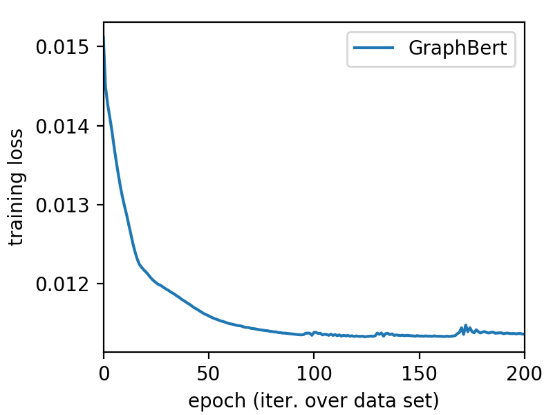
(a) Node Reconstruction

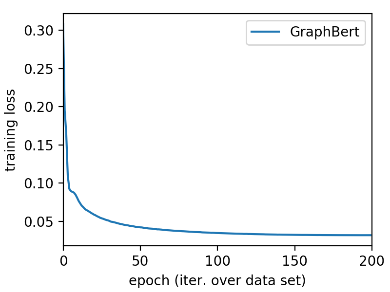
(b) Graph Recovery

Figure 2: Pre-training of Graph-Bert on node reconstruction and graph recovery tasks (x axis: iteration; y axis: training loss).

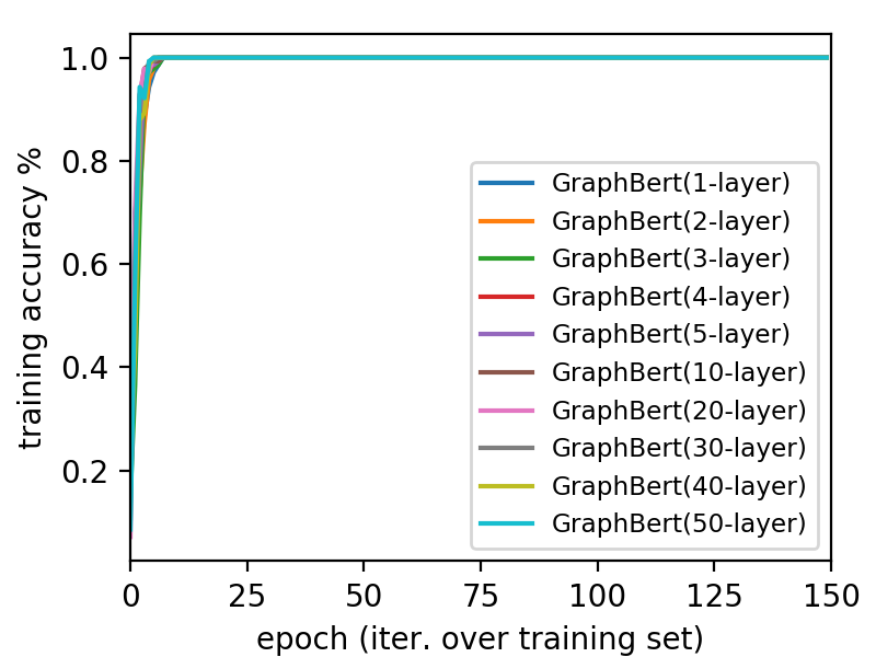
(a) Training Accuracy

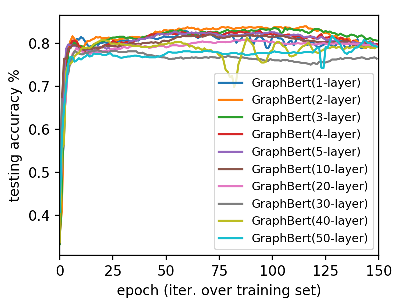
(b) Testing Accuracy

Figure 3: The learning performance of Graph-Bert on node classification with 1-layer, $\dotsc$, 5-layer, and 10-layer, $\cdots$, 50-layer on the Cora dataset. The x axis denotes the iterations over the whole training set. The y axes denote the training and testing accuracy, respectively.

Table 1: Learning Performance of Graph-Bert (based on different graph residual terms) compared against existing baseline methods on node classification. The results of Graph-Bert reported here denotes the best observed scores obtained with subgraph size $k\in\{1,2,\cdots,10,15,20,\cdots,50\}$.

Methods	Datasets (Accuracy)
	Cora	Citeseer	Pubmed
LP (Zhu et al. (2003))	0.680	0.453	0.630
ICA (Lu and Getoor (2003))	0.751	0.691	0.739
ManiReg (Belkin et al. (2006))	0.595	0.601	0.707
SemiEmb (Weston et al. (2008))	0.590	0.596	0.711
DeepWalk (Perozzi et al. (2014b))	0.672	0.432	0.653
Planetoid (Yang et al. (2016))	0.757	0.647	0.772
MoNet (Monti et al. (2016))	0.817	-	0.788
GCN (Kipf and Welling (2016))	0.815	0.703	0.790
GAT (Veličković et al. (2018))	0.830	0.725	0.790
LoopyNet (Zhang (2018))	0.826	0.716	0.792
Graph-Bert	0.843	0.712	0.793

Table 2: Analysis of subgraph size $k$ on Cora for model performance (testing accuracy and testing loss) and total time cost.

	Cora Dataset
k	Test Accuracy	Test Loss	Total Time Cost (s)
1	0.804	0.791	3.64
2	0.806	0.708	4.02
3	0.819	0.663	4.65
4	0.818	0.690	4.75
5	0.824	0.636	5.20
6	0.834	0.625	5.62
7	0.843	0.620	5.96
8	0.828	0.653	6.54
9	0.814	0.679	6.87
10	0.819	0.653	7.26
20	0.819	0.666	12.31
30	0.801	0.710	17.56
40	0.768	0.805	23.77
50	0.759	0.833	31.59

5.1 Dataset and Learning Settings

The graph benchmark datasets used in the experiments include Cora, Citeseer and Pubmed Yang et al. (2016), which are used in most of the recent state-of-the-art graph neural network research works Kipf and Welling (2016); Veličković et al. (2018); Zhang and Meng (2019). Based on the input graph data, we will first pre-compute the node intimacy scores, based on which subgraph batches will be sampled subject to the subgraph size $k\in\{1,2,\cdots,10,15,20,\cdots,50\}$. In addition, we will also pre-compute the node pairwise hop distance and WL node codes. By minimizing the node raw feature reconstruction loss and graph structure recovery loss, Graph-Bert can be effectively pre-trained, whose learned variables will be transferred to the follow-up node classification and graph clustering tasks with/without fine-tuning. In the experiments, we first pre-train Graph-Bert based on the node attribute reconstruction task with 200 epochs, then load and pre-train the same Graph-Bert model again based on the graph structure recovery task with another 200 epochs. In Figure 2, we show the learning performance of Graph-Bert on node attribute reconstruction and graph recovery, which converges very fast on both of these tasks.

Table 3: Learning performance of Graph-Bert with different graph residual terms.

Methods		Datasets (Accuracy)
Models	Residual	Cora	Citeseer	Pubmed
Graph-Bert	none	0.804	0.616	0.786
	raw	0.817	0.653	0.786
	graph-raw	0.843	0.712	0.793

Table 4: Learning performance of Graph-Bert with different initial embedding inputs.

Methods		Datasets (Accuracy)
Models	Embedding	Cora	Citeseer	Pubmed
Graph-Bert	hop distance	0.307	0.348	0.445
	position	0.323	0.331	0.395
	wl role	0.457	0.345	0.443
	raw feature	0.795	0.611	0.780
	all	0.804	0.616	0.786

Table 5: Clustering results of Graph-Bert without pre-training solely based on node raw features (MI: mutual information).

Metrics	Datasets
	Cora	Citeseer	Pubmed
Rand	0.080	0.249	0.281
Adjusted MI	0.130	0.287	0.313
Normalized MI	0.133	0.289	0.313
Homogeneity	0.133	0.287	0.280
Completeness	0.132	0.291	0.355

5.1.1 Default Parameter Settings

If not clearly specified, the results reported in this paper are based on the following parameter settings of Graph-Bert: subgraph size: $k=7$ (Cora), $k=5$ (Citeseer) and $k=30$ (Pubmed); hidden size: 32; attention head number: 2; hidden layer number: $D=2$; learning rate: 0.01 (Cora) and 0.001 (Citeseer) and 0.0005 (Pubmed); weight decay: $5e^{-4}$; intermediate size: 32; hidden dropout rate: 0.5; attention dropout rate: 0.3; graph residual term: graph-raw; training epoch: 150 (Cora), 500 (Pubmed), 2000 (Citeseer).

5.2 Node Classification without Pre-training

Graph-Bert is a powerful mode and it can be applied to address various graph learning tasks in the standalone mode. To show the effectiveness of Graph-Bert, we will first provide the experimental results of Graph-Bert on the node classification task without pre-training here, whereas the pre-trained Graph-Bert based node classification results will be provided in Section 5.4 in more detail. Here, we will follow the identical train/validation/test set partitions used in the existing graph neural network papers Yang et al. (2016) for fair comparisons.

5.2.1 Learning Convergence of Deep Graph-Bert

In Figure 3, we illustrate the training records of Graph-Bert for node classification on the Cora dataset. To show that Graph-Bert is different from other GNN models and Graph-Bert works with deep architectures, we also change the model depth with values from $\{1,2,\cdots,5,10,20,\cdot,50\}$. According to the plots, Graph-Bert can converge very fast (with less than 10 epochs) on the training set. What’s more, as the model depth increases, Graph-Bert will not suffer from the suspended animation problem. Even the very deep Graph-Bert (50 layers) can still respond effectively to the training data and achieve good learning performance.

5.2.2 Main Results

The learning results of Graph-Bert (with different graph residual terms) on node classification are provided in Table 1. The comparison methods used here cover both classic and state-of-the-art GNN models. For the variant models which extend GCN and GAT (with new learning settings, include more training data, re-configure the graph structure or use new optimization methods), we didn’t compare them here. However, similar techniques proposed by these extension works can be used to further help improve Graph-Bert as well. According to the achieved scores, we observe that Graph-Bert can out-perform most of these baseline methods with a big improvement on both Cora and Pubmed. On Citeseer, its perofrmance is also among the top 3.

Table 6: Performance comparison of Graph-Bert on fine-tuning tasks with/without pre-training. For all the models shown here, we will only use $\frac{1}{5}$ of the normal training max epochs as used by Graph-Bert in Table 1. For KMeans, the epoch denotes its max-iter parameter.

Methods		Datasets (Accuracy/Rand & Epoch)
Pre-Train Task	Fine-Tune Task	Cora		Citeseer		Pubmed
Node Reconstruction	Node Classification	0.827	30	0.649	400	0.780	100
	Graph Clustering	0.400	30	0.312	400	0.027	100
Structural Recovery	Node Classification	0.823	30	0.662	400	0.788	100
	Graph Clustering	0.123	30	0.090	400	0.132	100
Both	Node Classification	0.836	30	0.672	400	0.791	100
	Graph Clustering	0.177	30	0.203	400	0.159	100
None	Node Classification	0.805	30	0.654	400	0.786	100
	Graph Clustering	0.080	30	0.249	400	0.281	100

5.2.3 Subgraph Size $k$ Analysis

As illustrated in Table 2, we provide the learning performance analysis of Graph-Bert with different subgraph sizes, i.e., parameter $k$, on the Cora dataset. According to the results, parameter $k$ affects the learning performance of Graph-Bert a lot, since it defines how many nearby nodes will be used to define the nodes’ learning context. For the Cora dataset, we observe that the learning performance of Graph-Bert improves steadily as $k$ increases from $1$ to $7$. After that, as $k$ further increases, the performance will degrade dramatically. For the good scores with $k=1$, partial contributions come from the graph residual terms in Graph-Bert. The time cost of Graph-Bert increases as $k$ goes larger, which is very minor actually compared with other existing GNN models, like GCN and GAT. Similar results can be observed for the other two datasets, but the optimal $k$ are different.

5.2.4 Graph Residual Analysis

What’s more, in Table 3, we also provide the learning results of Graph-Bert with different graph residual terms. According to the scores, Graph-Bert with graph-raw residual term can outperform the other two, which is also consistent with the experimental observations on these different residual terms as reported in Zhang and Meng (2019).

5.2.5 Initial Embedding Analysis

As shown in Table 4, we provide the learning performance of Graph-Bert on these three datasets, which takes different initial embeddings as the input. To better show the performance differences, the Graph-Bert used here doesn’t involve any residual learning. According to the results, using the Weisfeiler-Lehman role embedding, hop based distance embedding and intimacy based positional embedding vectors along, Graph-Bert cannot work very well actually, whereas the raw feature embeddings do contribute a lot. Meanwhile, by incorporating such complementary embeddings into the raw feature embedding, the model can achieve better performance than using raw feature embedding only.

5.3 Graph Clustering without Pre-Training

In Table 5, we show the learning results of Graph-Bert on graph clustering without any pre-training on the three datasets. Formally, the clustering component used in Graph-Bert is KMeans, which takes the nodes’ raw feature vectors as the input. The results are evaluated with several different metrics shown above.

5.4 Pre-training vs. No Pre-training

The results reported in the previous subsections are all based on the Graph-Bert without pre-training actually. Here, we will provide the experimental results on Graph-Bert with pre-training to show their differences. According to the experiments, given enough training epochs, models with/without pre-training can both converge to very good learning results. Therefore, to highlight the differences, we will only use $\frac{1}{5}$ of the normal training epochs here for fine-tuning Graph-Bert, and the results are provided in Table 6. We also show the performance of Graph-Bert without pre-training here for comparison.

According to the scores, for most of the datasets, pre-training do give Graph-Bert a good initial state, which helps the model achieve better performance with only a very small number of fine-tuning epochs. On Cora and Citeseer, pre-training helps both the node classification and graph clustering tasks. Meanwhile, for Pubmed, pre-training helps node classification but degrades the results on graph clustering. Also pre-training with both node classification and graph recovery help the model to capture more information from the graph data, which also lead to higher scores than the models with single pre-training tasks.

6 Conclusion

In this paper, we have introduced the new Graph-Bert model for graph representation learning. Different from existing GNNs, Graph-Bert works well in deep architectures and will not suffer from the common problems with other GNNs. Based on a batch of linkless subgraphs sampled from the original graph data, Graph-Bert can effectively learn the representations of the target node with the extended graph-transformer layers introduced in this paper. Graph-Bert can serve as the graph representation learning component in graph learning pipeline. The pre-trained Graph-Bert can be transferred and applied to address new tasks either directly or with necessary fine-tuning.

References

- Adamic and Adar [2003] Eytan Adamic and Lada A. Adar. Friends and neighbors on the web. (3):211–230, July 2003.
- Belkin et al. [2006] Mikhail Belkin, Partha Niyogi, and Vikas Sindhwani. Manifold regularization: A geometric framework for learning from labeled and unlabeled examples. J. Mach. Learn. Res., 7:2399?2434, December 2006.
- Chung et al. [2014] Junyoung Chung, Çaglar Gülçehre, KyungHyun Cho, and Yoshua Bengio. Empirical evaluation of gated recurrent neural networks on sequence modeling. CoRR, abs/1412.3555, 2014.
- Dai et al. [2019] Zihang Dai, Zhilin Yang, Yiming Yang, Jaime G. Carbonell, Quoc V. Le, and Ruslan Salakhutdinov. Transformer-xl: Attentive language models beyond a fixed-length context. CoRR, abs/1901.02860, 2019.
- Devlin et al. [2018] Jacob Devlin, Ming-Wei Chang, Kenton Lee, and Kristina Toutanova. BERT: pre-training of deep bidirectional transformers for language understanding. CoRR, abs/1810.04805, 2018.
- Grover and Leskovec [2016] Aditya Grover and Jure Leskovec. node2vec: Scalable feature learning for networks. CoRR, abs/1607.00653, 2016.
- Gürel et al. [2019] Nezihe Merve Gürel, Hansheng Ren, Yujing Wang, Hui Xue, Yaming Yang, and Ce Zhang. An anatomy of graph neural networks going deep via the lens of mutual information: Exponential decay vs. full preservation. ArXiv, abs/1910.04499, 2019.
- Hamilton et al. [2017] William L. Hamilton, Rex Ying, and Jure Leskovec. Inductive representation learning on large graphs. CoRR, abs/1706.02216, 2017.
- Hammond et al. [2011] David K. Hammond, Pierre Vandergheynst, and Remi Gribonval. Wavelets on graphs via spectral graph theory. Applied and Computational Harmonic Analysis, 30(2):129?150, Mar 2011.
- He et al. [2018] Kaiming He, Ross B. Girshick, and Piotr Dollár. Rethinking imagenet pre-training. CoRR, abs/1811.08883, 2018.
- Hochreiter and Schmidhuber [1997] Sepp Hochreiter and Jürgen Schmidhuber. Long short-term memory. Neural Comput., 9(8), November 1997.
- Huang and Carley [2019] Binxuan Huang and Kathleen M. Carley. Inductive graph representation learning with recurrent graph neural networks. CoRR, abs/1904.08035, 2019.
- Jaccard [1901] Paul Jaccard. Étude comparative de la distribution florale dans une portion des alpes et des jura. Bulletin del la Société Vaudoise des Sciences Naturelles, 37:547–579, 1901.
- Jin et al. [2018] Wengong Jin, Regina Barzilay, and Tommi S. Jaakkola. Junction tree variational autoencoder for molecular graph generation. CoRR, abs/1802.04364, 2018.
- Katz [1953] Leo Katz. A new status index derived from sociometric analysis. Psychometrika, 18(1):39–43, Mar 1953.
- Kim [2014] Yoon Kim. Convolutional neural networks for sentence classification. In Proceedings of the 2014 Conference on Empirical Methods in Natural Language Processing (EMNLP), pages 1746–1751, Doha, Qatar, October 2014. Association for Computational Linguistics.
- Kipf and Welling [2016] Thomas N. Kipf and Max Welling. Semi-supervised classification with graph convolutional networks. CoRR, abs/1609.02907, 2016.
- Klicpera et al. [2018] Johannes Klicpera, Aleksandar Bojchevski, and Stephan Günnemann. Personalized embedding propagation: Combining neural networks on graphs with personalized pagerank. CoRR, abs/1810.05997, 2018.
- Lan et al. [2019] Zhenzhong Lan, Mingda Chen, Sebastian Goodman, Kevin Gimpel, Piyush Sharma, and Radu Soricut. Albert: A lite bert for self-supervised learning of language representations, 2019.
- Li et al. [2018] Qimai Li, Zhichao Han, and Xiao-Ming Wu. Deeper insights into graph convolutional networks for semi-supervised learning. CoRR, abs/1801.07606, 2018.
- Lu and Getoor [2003] Qing Lu and Lise Getoor. Link-based classification. In Proceedings of the Twentieth International Conference on International Conference on Machine Learning, ICML’03, page 496?503. AAAI Press, 2003.
- Meng and Zhang [2019] Lin Meng and Jiawei Zhang. Isonn: Isomorphic neural network for graph representation learning and classification. CoRR, abs/1907.09495, 2019.
- Monti et al. [2016] Federico Monti, Davide Boscaini, Jonathan Masci, Emanuele Rodolà, Jan Svoboda, and Michael M. Bronstein. Geometric deep learning on graphs and manifolds using mixture model cnns. CoRR, abs/1611.08402, 2016.
- Niepert et al. [2016] Mathias Niepert, Mohamed Ahmed, and Konstantin Kutzkov. Learning convolutional neural networks for graphs. CoRR, abs/1605.05273, 2016.
- Perozzi et al. [2014a] Bryan Perozzi, Rami Al-Rfou, and Steven Skiena. Deepwalk: Online learning of social representations. In Proceedings of the 20th ACM SIGKDD International Conference on Knowledge Discovery and Data Mining, KDD ’14, pages 701–710, New York, NY, USA, 2014. ACM.
- Perozzi et al. [2014b] Bryan Perozzi, Rami Al-Rfou, and Steven Skiena. Deepwalk: Online learning of social representations. CoRR, abs/1403.6652, 2014.
- Shang et al. [2019] Junyuan Shang, Tengfei Ma, Cao Xiao, and Jimeng Sun. Pre-training of graph augmented transformers for medication recommendation. CoRR, abs/1906.00346, 2019.
- Sun et al. [2019] Ke Sun, Zhouchen Lin, and Zhanxing Zhu. Adagcn: Adaboosting graph convolutional networks into deep models, 2019.
- Ugander et al. [2011] Johan Ugander, Brian Karrer, Lars Backstrom, and Cameron Marlow. The anatomy of the facebook social graph. CoRR, abs/1111.4503, 2011.
- Vaswani et al. [2017] Ashish Vaswani, Noam Shazeer, Niki Parmar, Jakob Uszkoreit, Llion Jones, Aidan N. Gomez, Lukasz Kaiser, and Illia Polosukhin. Attention is all you need. CoRR, abs/1706.03762, 2017.
- Veličković et al. [2018] Petar Veličković, Guillem Cucurull, Arantxa Casanova, Adriana Romero, Pietro Liò, and Yoshua Bengio. Graph Attention Networks. International Conference on Learning Representations, 2018.
- Weston et al. [2008] Jason Weston, Frédéric Ratle, and Ronan Collobert. Deep learning via semi-supervised embedding. In Proceedings of the 25th International Conference on Machine Learning, ICML’08, page 1168?1175, New York, NY, USA, 2008. Association for Computing Machinery.
- Yang et al. [2016] Zhilin Yang, William W. Cohen, and Ruslan Salakhutdinov. Revisiting semi-supervised learning with graph embeddings. CoRR, abs/1603.08861, 2016.
- Zhang and Meng [2019] Jiawei Zhang and Lin Meng. Gresnet: Graph residual network for reviving deep gnns from suspended animation. ArXiv, abs/1909.05729, 2019.
- Zhang et al. [2018] Jiawei Zhang, Limeng Cui, and Fisher B. Gouza. SEGEN: sample-ensemble genetic evolutional network model. CoRR, abs/1803.08631, 2018.
- Zhang [2018] Jiawei Zhang. Deep loopy neural network model for graph structured data representation learning. CoRR, abs/1805.07504, 2018.
- Zhu et al. [2003] Xiaojin Zhu, Zoubin Ghahramani, and John Lafferty. Semi-supervised learning using gaussian fields and harmonic functions. In Proceedings of the Twentieth International Conference on International Conference on Machine Learning, ICML’03, page 912?919. AAAI Press, 2003.