Voltage-Controlled Magnetic Reversal in Orbital Chern Insulators

Abstract

Chern insulator ferromagnets are characterized by a quantized anomalous Hall effect (QAHE), and have so far been identified experimentally in magnetically-doped topological insulator (MTI) thin films and in bilayer graphene moiré superlattices. We classify Chern insulator ferromagnets as either spin or orbital, depending on whether the orbital magnetization (OM) results from spontaneous spin-polarization combined with spin-orbit interactions, as in the MTI case, or directly from spontaneous orbital currents, as in the moiré superlattice case. We argue that in a given magnetic state, characterized for example by the sign of the anomalous Hall effect (AHE), the magnetization of an orbital Chern insulator will often have opposite signs for weak $n$ and weak $p$ electrostatic or chemical doping. This property enables pure electrical switching of a magnetic state in the presence of a fixed magnetic field.

Introduction— A ferromagnet may be defined as an equilibrium state of matter in which time-reversal (TR) symmetry is broken without lowering translational symmetries. Ferromagnets generically have both non-zero spin magnetization and non-zero OM. In almost all ferromagnets, the microscopic mechanism responsible for order is spontaneous spin-alignment driven by exchange interactions, which breaks spin-rotational invariance and leads to a non-zero spatially averaged spin moment density. Spin-orbit interactions then play a secondary role by inducing a small parasitic contribution to magnetization from orbital currents and a related non-zero (anomalous) Hall conductivity.

This Letter is motivated by recent experimentsChang et al. (2013); Sharpe et al. (2019); Chen et al. (a); Serlin et al. (2019); Polshyn et al. (a); Chen et al. (b) that have established the QAHE in two quite different classes of two-dimensional ferromagnets. The QAHE signalsThouless et al. (1982); Haldane (1988) the formation of a ferromagnetic state, often referred to as a Chern insulator, with occupied quasiparticle bands whose topological Chern numbersXiao et al. (2010) sum to a non-zero value. We find that when ferromagnetism mainly results from spontaneous orbital moments (not spin moments), as in the QAHE states recently discoveredSharpe et al. (2019); Chen et al. (a); Serlin et al. (2019) in magic angle twisted bilayer graphene (MATBG), the magnetizations of weakly $n$-doped and weakly $p$-doped insulators can differ in sign in the same magnetic state characterized for example by a given sign of the anomalous Hall conductivity. This property could enable magnetic state reversal in the presence of a magnetic field to be achieved purely electrically.

The mechanism that allows the magnetizations of weakly $n$-doped and weakly $p$-doped Chern insulators to differ drastically is closely related to the quantum Hall effect itself. Because of the presence of protected edge states, the OM $M$ of a Chern insulator changesMacDonald with chemical potential $\mu$ even when $\mu$ is inside the bulk energy gap:

$$\frac{dM}{d\mu}=\frac{dI}{d\mu}=\frac{Ce}{2\pi\hbar},$$ (1)

where $C$, the Chern index sum, is an integer equal to the Hall conductance in $e^{2}/h$ units. Eq. (1) emphasizes that the quantized Hall conductance can be understoodMacDonald in terms of chiral edge states that are occupied to different chemical potentials along different portions of the sample boundary. It follows from Eq. (1) that the magnetization jumps by

$$\Delta{M}=\frac{CeE_{\text{gap}}}{2\pi\hbar}$$ (2)

when the chemical potential jumps across the gap of a Chern insulator. Note that the jump in the magnetization depends only on the value of the energy gap and on fundamental constants. We show below that in orbital Chern insulator ferromagnets this jump can be sufficient to change the sign of magnetization simply by changing the sign of doping.

Spin Chern Insulators— In MTI thin films, TR symmetry is broken by introducing local moments that order ferromagnetically. Spin-orbit coupling then leads to an AHE that is quantized, and to orbital ferromagnetism. To compare the OM jump with the magnitude of the spin magnetization, we express it in units of Bohr magnetons $\mu_{\text{B}}=e\hbar/2m$ per surface unit cell:

$$\frac{\Delta M}{\mu_{\text{B}}/A_{\text{uc}}}=\frac{CmA_{\text{uc}}E_{\text{gap}}}{\pi\hbar^{2}}$$ (3)

where $A_{\text{uc}}$ is the area of the surface unit cell. In MTIs, spin magnetization in Bohr magnetons per surface unit cell is typically $\sim 1$, because the fraction of sites with magnetic atoms is $\sim 0.1$ and the number of magnetically doped layers is $\sim 10$. Note that the spin magnetization does not depend on the position of the chemical potential within the gap. We see from Eq. (3) that the OM jump across the gap is small compared with the spin magnetization since the surface state energy gap, although not known accurately, is certainly small compared to the $\hbar^{2}/mA_{\text{uc}}$, which depends only on fundamental constants and the surface unit cell area and has a typical value in the $1-10$ eV range. For MTIs, and other spin Chern insulators, the unusual jump in the magnetization across the insulator’s gap is small in a relative sense and unlikely to have a qualitative influence on magnetic properties.

Orbital Chern Insulators— The Hall conductivity of a Chern insulator ferromagnet is quantized when the chemical potential lies in the gap or when carriers introduced by chemical or electrostatic doping are localized. It is convenient to use the sign of the Hall conductivity to distinguish a magnetic state from its TR counterpart. We will refer to the state with positive quantized Hall conductivity $Ce^{2}/h$ as the $+$ state and to the state with negative quantized Hall conductivity $-Ce^{2}/h$ as the $-$ state. Although their variations with chemical potential are very distinct, as we emphasize below, both the Hall conductivity $\sigma_{\text{H}}^{\pm}(\mu)$ and OM $M^{\pm}(\mu)$ are orbital fingerprints of broken TR and at any doping level have opposite signs in TR partner states: $M^{-}(\mu)=-M^{+}(\mu),\ \sigma_{\text{H}}^{-}(\mu)=-\sigma_{\text{H}}^{+}(\mu).$

The TR symmetry breaking mechanism active in the orbital Chern insulators recently discovered in MATBG devices has been actively discussed in recent workBultinck et al. (2020); Repellin et al. (2020); Zhang et al. (2019); Wu and Das Sarma (2020); Alavirad and Sau ; Liu and Dai . It is almost certainly related to condensation in momentum space, a concept discussed some time ago by Heisenberg and LondonLondon (1948) and previously proposedJung et al. (2015a) as a possible symmetry breaking mechanism in metallic gated AB Bernal bilayer graphene. Momentum space condensation is driven by the property that interaction energies in systems with long-range Coulomb interactions can be lowered by occupying states that are more compactly distributed in momentum space than the occupied states of non-interacting bands. Just as exchange interactions in itinerant electron systems occur only between like spins, exchange interactions between states with nearby momenta are stronger than those between states far apart in momentum space. In materials, like graphene, with low energy states located near two widely separated valley centers, momentum space condensation translates to spontaneous valley population polarization. When combined with the intrinsically topological characterPo et al. (2019); Song et al. (2019); Lu et al. (2019) of the valley-projected bands in these materials, valley polarization yields an AHE that is quantized in insulating states. The recently discovered graphene multilayer QAHE statesSharpe et al. (2019); Chen et al. (a); Serlin et al. (2019) provide, as far as we are aware, the only demonstrated example of this mechanism at work. In order to estimate the OM of these states we apply the convenient envelope function descriptionBistritzer and MacDonald (2011), in which the moiré superlattices is described by a valley-projected periodic Hamiltonian that accounts for position-dependent stacking. We focus below on the case of twisted bilayer graphene (TBG) sandwiched by aligned hexagonal Boron Nitride (hBN) layers.

OM of MATBG on hBN— The contribution to OM from a single band of 2D Bloch electrons isXiao et al. (2010); Thonhauser et al. (2005); Ceresoli et al. (2006); Bianco and Resta (2013, 2016)

$$M_{n}(\mu) = \int\frac{d^{2}\boldsymbol{k}}{(2\pi)^{2}}\mathcal{M}_{n}(\boldsymbol{k},\mu)f(\mu-\varepsilon_{n}(\boldsymbol{k}))$$ (4)

$$\mathcal{M}_{n}(\boldsymbol{k},\mu) = \frac{e}{\hbar}\text{Im}\sum\limits_{n^{\prime}\neq n}\frac{\langle n|\partial_{x}H|n^{\prime}\rangle\langle n^{\prime}|\partial_{y}H|n\rangle}{(\varepsilon_{n}-\varepsilon_{n^{\prime}})^{2}}\,(\varepsilon_{n}+\varepsilon_{n^{\prime}}-2\mu)$$

where $n$ is a band index, $\mu$ is the chemical potential, $f(\mu-\varepsilon_{n}(\boldsymbol{k}))$ is Fermi-Dirac distribution, $\partial_{j}H=\partial H/\partial k_{j}$ is the velocity operator and $|n\rangle$ is a Bloch state with implicit wave-vector dependence. We separate the OM in Eq. (4) into two parts by defining

$$M_{n}^{1}(\mu) = \frac{e}{\hbar}\text{Im}\sum\limits_{n^{\prime}\neq n}\int\frac{d^{2}\boldsymbol{k}f_{n}}{(2\pi)^{2}}\frac{\langle n|\partial_{x}H|n^{\prime}\rangle\langle n^{\prime}|\partial_{y}H|n\rangle}{(\varepsilon_{n}-\varepsilon_{n^{\prime}})^{2}}(\varepsilon_{n}+\varepsilon_{n^{\prime}})$$

$$M_{n}^{2}(\mu) = \frac{e}{\hbar}\text{Im}\sum\limits_{n^{\prime}\neq n}\int\frac{d^{2}\boldsymbol{k}f_{n}}{(2\pi)^{2}}\frac{\langle n|\partial_{x}H|n^{\prime}\rangle\langle n^{\prime}|\partial_{y}H|n\rangle}{(\varepsilon_{n}-\varepsilon_{n^{\prime}})^{2}}(-2\mu)$$ (5)

where $f_{n}$ is short for $f(\mu-\varepsilon_{n}(\boldsymbol{k}))$. When band $n$ is full, $M_{n}^{1}(\mu)$ is independent of $\mu$, whereas $M_{n}^{2}(\mu)$ includes the edge state contribution and is proportional to $\mu$ with proportionality constant $C_{n}e/2\pi\hbar$, where $C_{n}$ is the Chern number of band $n$.

We now apply these expressions to TBG encapsulated between hBN layers whose influence on the low-energy graphene Hamiltonian is capturedWallbank et al. (2013); Moon and Koshino (2014); Jung et al. (2015b, 2017, 2014); Kindermann et al. (2012); Shi et al. in part by a mass term representing the spatially averaged difference between carbon $\pi$-orbital energies on different honeycomb sublattices. The valley-projected TBG Hamiltonian is $\mathcal{H}(\boldsymbol{r})=h_{0}^{(1)}+h_{0}^{(2)}+T(\boldsymbol{r})+h.c.$, where $h_{0}^{(l)}(\boldsymbol{r})=-i\partial_{x}\sigma_{x}-i\partial_{y}\sigma_{y}+m_{l}\sigma_{z}$ is the massive Dirac Hamiltonian of layer $l$, $\sigma$ acts on the sublattice degrees of freedom, and $T(\boldsymbol{r})$ is the periodic interlayer tunneling HamiltonianBistritzer and MacDonald (2011). The conclusions we reach below rest in part on a particle-hole symmetry property of this Hamiltonian, discussed at greater length in supplementary material (SM) S1.

$$\tau_{z}\sigma_{x}\mathcal{H}(x,y)\sigma_{x}\tau_{z}=-\mathcal{H}(-x+d,y)$$ (6)

$$\tau_{x}\mathcal{H}(x,y)\tau_{x}=\mathcal{H}^{*}(-x+d,y)$$ (7)

In Eqs. (6,7), $\tau$ acts on the layer degrees of freedom and $d=a_{\text{\tiny{M}}}/\sqrt{3}$ (modulo $\sqrt{3}a_{\text{\tiny{M}}}$) where $a_{\text{\tiny{M}}}$ is moiré lattice constant. Symmetry (6) states that up to a translation and a change in the sign of the interlayer tunneling term, sublattice exchange combined with reflection by the $y$-axis simply changes the sign of the Hamiltonian. Eq. (6) becomes exact in the limit of small twist angles and is accurate in MATBG. Eq. (7) is satisfied only when the masses of two graphene layers are identical. In momentum space, the Hamiltonian satisfies

$$\tau_{z}\sigma_{x}H(k_{x},k_{y})\sigma_{x}\tau_{z}=-H(-k_{x},k_{y})$$ (8)

$$\tau_{x}H(k_{x},k_{y})\tau_{x}=H^{*}(k_{x},-k_{y})$$ (9)

Given Eq. (8) it can be shown, as detailed in SM S1, that the contribution to OM from a valley vanishes when $\mu$ lies in the middle of the gap between the conduction and valence bands of that valley.

For graphene on hBN $m$ has been estimated using DFTJung et al. (2015b, 2017, 2014) to be $\sim 3.6$ meV for perfect alignment, but can be substantially enhanced by interaction effects absent in DFT and decreases with relative twist angle. Experimental $m$ values for nearly aligned graphene on hBN are $\sim$ 10$-$15 meVRebeca et al. (2018); Hunt et al. (2013); Finney et al. (2019). Figure 1 illustrates the $K$-valley low-energy moiré bands and Chern numbers of $1.1^{\circ}$-TBG for different mass choices. The choice $m_{1}=m_{2}$ (Fig.1(a)) corresponds to the case in which both graphene layers are aligned and have equivalent stacking orientation relative to their adjacent hBN layers, while $m_{1}=-m_{2}$ (Fig.1(c)) corresponds to the case in which two graphene layers have opposite relative stacking orientations. $m_{l}=0$ (Fig.1(b)) corresponds to layer $l$ having a large misalignment relative to hBN so that strain enhancement is absent. We find that gaps ($E_{\text{g}}^{0}$) appear at charge neutrality, that the bands are relatively flat for twists near the magic angle, and that they have non-zero Chern numbers when both layers have the same alignment or only one layer is aligned. The case of opposite masses produces trivial bands (Fig. 1(c)). In all three cases sublattice-symmetry breaking gaps the Dirac points at the moiré Brillouin zone (MBZ) corners that otherwise link the conduction and valence bands.

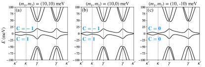
Figure 1: $1.1^{\circ}$-TBG moiré band structures in valley $K$ for three hBN-induced mass choices. (a) $m_{1}=m_{2}=10$ meV produces a band gap $E_{\text{g}}^{0}\sim 7.5$ meV at charge neutrality. The flat bands are non-trivial with Chern numbers $C=\pm 1$. (b) $m_{1}=10,m_{2}=0$ meV produces a band gap $E_{\text{g}}^{0}\sim 2.3$ meV. The flat bands are non-trivial with Chern numbers $C=\pm 1$. (c) $m_{1}=-m_{2}=-10$ meV produces a band gap $E_{\text{g}}^{0}\sim 3$ meV with topologically trivial flat bands. The moiré bands were calculated using a low-energy continuum modelBistritzer and MacDonald (2011) with interlayer tunneling strength $w^{\scaleto{\text{AB}}{4pt}}=110$ meV and $w^{\scaleto{\text{AA}}{4pt}}/w^{\scaleto{\text{AB}}{4pt}}=0.85$ to account for corrugation and strain.

SU(4) symmetric mean-field model— Figure  2(b) plots the single-flavor magnetization contributions (solid line) from valleys $K$ and $K^{\prime}$ at twist angle $1.1^{\circ}$ as a function of $\mu$ measured relative to the mid-point between its shifted conduction and valence bands. As explained previously the magnetization contribution from each valley vanishes at mid-gap and varies linearly within the gap. Because valleys $K$ and $K^{\prime}$ are time-reversed counterparts, their magnetization contributions are always opposite in sign. The dotted and dash-dotted lines in Fig. 2(b) separate the $M^{1}$ and $M^{2}$ contributions defined in Eq. (Voltage-Controlled Magnetic Reversal in Orbital Chern Insulators). The range of $\mu$ plotted in Fig. 2(b) covers from the flat valence band bottom to the flat conduction band topfoo .

Because of the four-fold spin/valley degeneracy of the moiré flat bands (Fig. 2(a)), gaps can appear only at moiré filling factors $\nu$ that are multiples of four when interactions are neglected. To account for the Chern insulator gaps at odd integer values of $\nu$, we use a simplified but still qualitatively reliableXie and MacDonald (2020) mean-field model in which exchange interactions shift all the band energies of a given flavor en masse – down when the flat conduction band is occupied and up when the flat valence band is emptied (Fig. 2(c-f)). The band energy shift $U$ must exceed the band width $w$ in order for the gapped state to be self-consistent; this Stoner criterion is easily satisfied near magic angle orientations because $w$ is extremely small. Schematic ordered state bands for $\nu=3$ and $\nu=1$ are plotted in Fig. 2(c) and (e). For three electrons per moiré period ($\nu=3$), the density at which the QAHE has been most often observed to date, all the majority $\downarrow$ spin’s flat bands are occupied and the magnetization contributions from its two valleys cancel. We can therefore consider only the minority $\uparrow$ spin bands shown in Fig. 2(d). Similarly, for one electron per moiré period ($\nu=1$), we can consider only the majority $\downarrow$ spin bands illustrated in Fig. 2(f).

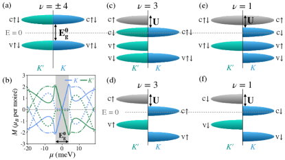
Figure 2: (a) Schematic moiré flat bands with SU(4) spin/valley symmetry maintained. Each band has a four-fold degeneracy. $E_{g}^{0}$ is the single-particle band gap. ”c” and ”v” are shorts for ”conduction” and ”valence” bands. (b) Magnetization contributions (solid line) from valleys $K$ (blue) and $K^{\prime}$ (green) as a function of $\mu$. The dotted and dash-dotted lines are respectively the $M^{1}$ and $M^{2}$ contributions defined in Eq. (Voltage-Controlled Magnetic Reversal in Orbital Chern Insulators). The single-particle gap is shaded in gray. (c-f) Schematic moiré flat bands in TR broken symmetry states at $\nu=3$ and $\nu=1$ in which different flavors are rigidly shifted in energy by a momentum- and flavor-independent exchange energy $U$ if the flat conduction band is filled in that flavor.

Although the magnetization of an orbital Chern insulator can in principle reverse its sign at any filling factor, depending on the details of the Chern band, abrupt reversals vs. gate voltage occur only at integer $\nu$, where the magnetization has a large jump. We, therefore, focus on the magnetization jumps at $\nu=3$ and $\nu=1$; a similar analysis applies for $\nu=-3$ and $\nu=-1$. The total OM is calculated by summing Eq. (4) over spin/valley flavors and bands:

$$M(\mu)=\sum\limits_{m,f}\big{(}M^{1}_{mf}n_{mf}+\mu\frac{C_{mf}n_{mf}}{2\pi}\big{)}+U\sum\limits_{m,f\in f_{\text{shift}}}\frac{C_{mf}n_{mf}}{2\pi}$$ (10)

where $m$ is a band index in the valley- and spin-projected continuum model, $f$ is a flavor index, $f_{\text{shift}}$ is the set of flavors that have had their energies shifted by $-U$, $n_{mf}$ is the band occupation, and $C_{mf}$ is the band Chern number. $M^{1}_{mf}$ is evaluated with the zero of energy located at the middle of the single-particle gap $E_{g}^{0}$ as in Fig. 2(a). In the last term in Eq.(10), we have used that the magnetization contribution of an occupied band changes by $-C_{mf}\delta E/2\pi$ when the band energy is rigidly shifted by $\delta E$.

Since the magnetizations and Chern numbers of time-reversed bands cancel, i.e. $M^{1}_{mK}$ $=$ $-M^{1}_{mK^{\prime}}$ and $C_{mK}=-C_{mK^{\prime}}$, it follows that at both $\nu=3$ and $\nu=1$

$$\sum\limits_{m,f}\big{(}M^{1}_{mf}n_{mf}+\mu\frac{C_{mf}n_{mf}}{2\pi}\big{)}=M^{1}_{\text{c}K}+\frac{\mu C_{\text{c}K}}{2\pi}.$$ (11)

The extra magnetization contribution from occupied bands that suffer an exchange energy shift $U$ is

$$U\sum\limits_{m,f\in f_{\text{shift}}}\frac{C_{mf}n_{mf}}{2\pi}=\frac{U(C_{\text{c}K}+C_{\text{v}K}+C_{\text{v}^{\prime}K})}{2\pi}$$ (12)

where $C_{\text{c}K}$/$C_{\text{v}K}$ is the Chern number of the flat conduction/valence band in valley $K$ and $C_{\text{v}^{\prime}K}$ is the total Chern number summed over all remote valence bands.

In our simplified SU(4) symmetric model, $M^{1}_{\text{c}K}$ and the Chern numbers are purely single-particle properties. For the range of parameters ($\theta$, $m$) plotted in Fig. 3, $C_{\text{c}K}$=$-C_{\text{v}K}$=$-1$ and $C_{\text{v}^{\prime}K}=0$. It follows that for both $\nu=1$ and $\nu=3$, the magnetization ($M^{\text{n-doped}}$) when $\mu$ is at the bottom of unoccupied band(s) is

$$M^{\text{n-doped}}=M(\mu=\frac{E_{g}}{2})=M^{1}_{\text{c}K}-\frac{E_{g}}{4\pi}$$ (13)

and the magnetization ($M^{\text{p-doped}}$) when $\mu$ is at the top of occupied bands is

$$M^{\text{p-doped}}=M(\mu=\frac{E_{g}}{2}-\Delta_{g})=M^{1}_{\text{c}K}-\frac{E_{g}}{4\pi}+\frac{\Delta_{g}}{2\pi}$$ (14)

where $\Delta_{g}=\text{min}\{U-w,E_{g}\}$ is the correlated gap at $\nu=1,3$. The magnetization sign reverses across the gap if

$$M^{\text{n-doped}}<0\text{ and }M^{\text{p-doped}}>0$$ (15)

In Fig.3(a) we show that $M^{1}_{\text{c}K}$ increases as a function of both twist angle $\theta$ and mass $m=m_{1}=m_{2}$. Figure 3(b), which plots $M^{\text{n-doped}}(\theta,m)$, reveals that the first condition in Eq.(15) is always satisfied near the magic twist angle. Figure 3(c) plots $M^{\text{p-doped}}$ for a typical twist angle $\theta=1.1^{\circ}$ vs. $U$ and mass $m$. Insulating states occur only when $U>w$. We find that $M^{\text{p-doped}}$ is almost always positive, satisfying the second condition in Eq.(15), although there is a small no-reversal region in which the Chern insulator gap $\Delta_{g}=U-w\sim 1$ meV that is highlighted in Fig. 3(d). Similar results for $m_{1}=m,m_{2}=0$ models are provided in Fig. 3(e-h). In this case, $M^{\text{n-doped}}$ is negative for $\theta\lesssim 1.04^{\circ}$, as illustrated in Fig.3(g).

Discussion— Chern insulators are 2D electron systems with charge gaps that exhibit QAHE, and have now been realized experimentally by two distinct mechanisms. In MTIChang et al. (2013); Checkelsky et al. (2014); Kou et al. (2014); Bestwick et al. (2015); Chang et al. (2015); Mogi et al. (2015); Jiang et al. , the QAHE is driven by the exchange interactions between spin-local-moments that order ferromagnetically and two Dirac-cones localized on opposite surfaces of a topological insulator thin film. In bilayer graphene, on the other hand, the QAHE is driven by broken sublattice symmetry, which gaps Dirac cones and induces Berry curvatures of opposite signs near TR-partner valleys, combined with TR symmetry breaking via condensation of electrons into one of the two valleys. Both experimentally established QAHE mechanisms differ from the one identified in the original theoretical work of HaldaneHaldane (1988) in which the QAHE is driven by broken TR symmetry that leads to Berry curvatures of the same sign near opposite valleys.

In TBG sublattice polarization is theoretically expected to occur spontaneously, but can be enforced by alignment with hBN. Spontaneous valley polarization and spin polarization are then energetically preferred when the moiré bands are narrowed by tuning the orientation close to the magic angle. Because of the absence of substantial spin-orbit coupling in graphene, the orbital valley order has Ising character and is therefore essential to achieve a finite transition temperature, and is dominantly responsible for the magnetization and solely responsible for the most accessible observable – the QAHE. We have shown in this Letter that the dominance of orbital magnetism change the considerationsDieny and Chshiev (2017) that normally limit our ability to control magnetic states electrically. The most extreme example of the strong electrical effects that are possible in orbital Chern insulators is a consequence of the jump in magnetization between weak $n$-doping and weak $p$-doping produced by edge states. Changing the sign of magnetization of a state with a given sign of valley polarization and QAHE, changes the thermodynamically preferred state in a weak magnetic field purely electrically. This property could be of technological value if other examples of orbital Chern insulators that have higher transition temperatures are discovered in the future. When the sign of the magnetization is independent of carrier density, the StředaStreda (1982a) formula implies that magnetic-switching between quantum anomalous Hall states will yield stronger transport signals for either $n$- or $p$-doping, depending on the relative sign of magnetization and Hall conductivity. This behavior is common in current experimentsChen et al. (a); Serlin et al. (2019); Lu et al. (2019); Wang et al. ; Stepanov et al. . As illustrated in SM S3 QAHE sign switching that is equally robust for $n$- and $p$-doping signals the magnetization sign switch that we expect to be common in large gap orbital Chern insulators.

In our simplified mean-field theory the magnetizations at weak $n$- and $p$-doping are identical at $\nu=3$ and $\nu=1$ since Eqs.(10-14) apply to both cases. This property is a consequence not only of the simplified mean-field theory but also of our neglect of correlations, which are likely to play an important role in determining whether or not Chern insulator states appear. Since the flat-band system has more phase space for correlations closer to charge neutrality, we anticipate that Chern insulator states will be more common at $\nu=\pm 3$, than at $\nu=\pm 1$.

Note added: While this manuscript was under review, the magnetization sign reversal it predicts was observed in twisted monolayer on bilayer graphene and in twisted bilayer graphenePolshyn et al. (b).

Acknowledgements— JZ was supported by the National Science Foundation through the Center for Dynamics and Control of Materials: an NSF MRSEC under Cooperative Agreement No. DMR-1720595. AHM was supported by DOE BES grant FG02-02ER45958. The authors acknowledge resources provided by the Texas Advanced Computing Center (TACC) at The University of Texas at Austin that have contributed to the research results reported in this paper.

Figure 3: Plots of $M^{1}_{\text{c}K}$, $M^{\text{n-doped}}$ and $M^{\text{p-doped}}$ defined in Eq. (11), (13) and (14). (a-d) With $m_{1}=m_{2}=m$. (e-g) With $m_{1}=m$ and $m_{2}=0$. (a) $M^{1}_{\text{c}K}$ increases as both twist angle $\theta$ and $m$. (b) $M^{\text{n-doped}}(\theta,m)$ is negative in most parts of the parameter range shown in the figure. (c) $M^{\text{p-doped}}(U,m)$ for a typical twist angle $\theta=1.1^{\circ}$. (d) Zoom-in of the dashed rectangle in (c). $M^{\text{p-doped}}$ is positive as long as $\Delta_{g}\gtrsim 1$ meV, which is easily achievable in MATBG. (e) Similar to (a), $M^{1}_{\text{c}K}$ increases as both $\theta$ and $m$. (f) $M^{\text{n-doped}}(\theta,m)$. (g) Zoom-in of the dashed rectangle in (f). $M^{\text{n-doped}}$ is only negative for $\theta\lesssim 1.04^{\circ}$. (h) $M^{\text{p-doped}}(U,m)$ for $\theta=1.02^{\circ}$. Similar to (d), $M^{\text{p-doped}}$ is positive for a tiny gap. In (c,d,h), the parameter region where $U<w$ is identified to be metallic.

I Supplemental Material:
The Curious Magnetic Properties of Orbital Chern Insulators

II S1. Symmetries of TBG

Below we prove that the moiré Hamiltonian $\mathcal{H}(\boldsymbol{r})$ of TBG on hBN substrates has the following symmetry properties:

$$\tau_{z}\sigma_{x}\mathcal{H}(x,y)\sigma_{x}\tau_{z}=-\mathcal{H}(-x+d,y)\ \ \ \ \ \ \ \ \$$ (16)

$$\tau_{x}\mathcal{H}(x,y)\tau_{x}=\mathcal{H}^{*}(-x+d,y)\ \ \ \ \ \ \ \ \ \ \ \ \ \ \ \ \ \ .$$ (17)

The first of these properties applies only in the limit of small twist angles and the second only if the Dirac masses $m_{1}$ and $m_{2}$ in the two layers are identical. The Pauli matrices $\sigma$ and $\tau$ act on sublattice and layer degrees of freedom respectively.

The moiré Hamiltonian

$$\mathcal{H}(\boldsymbol{r})=\begin{pmatrix}h_{0}^{(1)}(\boldsymbol{r})&T(\boldsymbol{r})\\ T^{\dagger}(\boldsymbol{r})&h_{0}^{(2)}(\boldsymbol{r})\end{pmatrix}$$ (18)

$T(\boldsymbol{r})$ is the interlayer tunneling matrices and superscripts $(1)$ and $(2)$ denote graphene layers. $h_{0}(\boldsymbol{r})$ is the massive Dirac Hamiltonian

$$h_{0}(x,y)=-i\partial_{x}\sigma_{x}-i\partial_{y}\sigma_{y}+m\sigma_{z}$$ (19)

and we have

$$\sigma_{x}h_{0}(x,y)\sigma_{x}=-h_{0}(-x,y)$$ (20)

For the interlayer tunneling term,

$$T(\boldsymbol{r})=w_{0}\sum\limits_{j=1}^{3}e^{-i\boldsymbol{q}_{j}\cdot\boldsymbol{r}}T_{j}$$ (21)

where $\boldsymbol{q}_{1}=(0,-1),\boldsymbol{q}_{2}=(\sqrt{3}/2,1/2),\boldsymbol{q}_{3}=(-\sqrt{3}/2,1/2)$ (in units of $4\pi/3a_{\text{\tiny{M}}}$) are three momentum boosts. $a_{\text{\tiny{M}}}$ is the moiré lattice constant. $w_{0}=110$ meV is the tunneling strength, and

$$T_{1}=\begin{pmatrix}1&1\\ 1&1\end{pmatrix},\ \ \ \ \ T_{2}=\begin{pmatrix}e^{-i\phi}&1\\ e^{i\phi}&e^{-i\phi}\end{pmatrix},\ \ \ \ \ T_{3}=\begin{pmatrix}e^{i\phi}&1\\ e^{-i\phi}&e^{i\phi}\end{pmatrix}$$ (22)

with $\phi=2\pi/3$. Substituting $\boldsymbol{q}_{j}$ and $T_{j}$ in Eq. (21),

$$T(-x+d,y)=e^{-i\boldsymbol{q}_{1}\cdot\boldsymbol{r}}\sigma_{x}T_{1}\sigma_{x}+e^{-i\boldsymbol{q}_{2}\cdot\boldsymbol{r}}e^{i(2\phi+q_{\text{\tiny{2x}}}d)}\sigma_{x}T_{2}\sigma_{x}+e^{-i\boldsymbol{q}_{3}\cdot\boldsymbol{r}}e^{e^{i(\phi-q_{\text{\tiny{2x}}}d)}}\sigma_{x}T_{3}\sigma_{x}$$ (23)

$$\sigma_{x}T(x,y)\sigma_{x}=e^{-i\boldsymbol{q}_{1}\cdot\boldsymbol{r}}\sigma_{x}T_{1}\sigma_{x}+e^{-i\boldsymbol{q}_{2}\cdot\boldsymbol{r}}\sigma_{x}T_{2}\sigma_{x}+e^{-i\boldsymbol{q}_{3}\cdot\boldsymbol{r}}\sigma_{x}T_{3}\sigma_{x}$$ (24)

and we get

$$\sigma_{x}T(x,y)\sigma_{x}=T(-x+d,y)$$ (25)

where $d=a_{\text{\tiny{M}}}/\sqrt{3}$ modulo $\sqrt{3}a_{\text{\tiny{M}}}$. In other words sublattice-exchange of the tunneling Hamiltonian is equivalent to reflection by the $y$-axis combined with a translation. Combining Eq. (20) and (25), we obtain

$$\tau_{z}\sigma_{x}\mathcal{H}(x,y)\sigma_{x}\tau_{z}=-\mathcal{H}(-x+d,y)$$ (26)

Similarly,

$$T^{\dagger}(x,y)=e^{i\boldsymbol{q}_{1}\cdot\boldsymbol{r}}T_{1}+e^{i\boldsymbol{q}_{2}\cdot\boldsymbol{r}}e^{-i\phi}T_{2}+e^{i\boldsymbol{q}_{3}\cdot\boldsymbol{r}}e^{i\phi}T_{3}$$ (27)

$$T^{*}(-x+d,y)=e^{i\boldsymbol{q}_{1}\cdot\boldsymbol{r}}T_{1}+e^{i\boldsymbol{q}_{2}\cdot\boldsymbol{r}}e^{-iq_{\text{\tiny{2x}}}d}T_{2}+e^{i\boldsymbol{q}_{3}\cdot\boldsymbol{r}}e^{iq_{\text{\tiny{2x}}}d}T_{3}$$ (28)

$$T^{\dagger}(x,y)=T^{*}(-x+d,y)$$ (29)

$d=a_{\text{\tiny{M}}}/\sqrt{3}$. If $m_{1}=m_{2}$, then

$$\tau_{x}\mathcal{H}(x,y)\tau_{x}=\mathcal{H}^{*}(-x+d,y)$$ (30)

Applying Bloch’s theorem to Eq. (16,17), we see that $H(\boldsymbol{k})$ satisfies

$$\tau_{z}\sigma_{x}H(k_{x},k_{y})\sigma_{x}\tau_{z}=-H(-k_{x},k_{y})$$ (31)

$$\tau_{x}H(k_{x},k_{y})\tau_{x}=H^{*}(k_{x},-k_{y})$$ (32)

As a result of Eq. (31), the eigenvalues and eigenvectors satisfy $\varepsilon_{\text{c}_{i}}(k_{x},k_{y})=-\varepsilon_{\text{v}_{i}}(-k_{x},k_{y})$, $\psi_{\text{c}_{i}}(k_{x},k_{y})=\tau_{z}\sigma_{x}\psi_{\text{v}_{i}}(-k_{x},k_{y})$. Here $i=1,2,...$ labels the $i$-th conduction (c_i) or valence (v_i) band counting from charge neutrality. For Eq. (32), $\varepsilon_{n}(k_{x},k_{y})=\varepsilon_{n}(k_{x},-k_{y})$, $\psi_{n}(k_{x},k_{y})=\tau_{x}\psi^{*}_{n}(k_{x},-k_{y})$, where $n$ label bands.

Now let us define the orbital magnetization contribution due to mixing between bands $n$ and $n^{\prime}$:

$$\mathfrak{M}^{nn^{\prime}}=\frac{e}{\hbar}\text{Im}\int_{\text{\tiny{MBZ}}}\frac{d^{2}\boldsymbol{k}}{(2\pi)^{2}}\frac{\langle n|\partial_{x}H|n^{\prime}\rangle\langle n^{\prime}|\partial_{y}H|n\rangle}{(\varepsilon_{n}-\varepsilon_{n^{\prime}})^{2}}(\varepsilon_{n}+\varepsilon_{n}^{\prime})$$ (33)

When the chemical potential at neutrality is in the middle of the gap, and the Hamiltonian has been truncated to a finite number ($2N$) of bands via a plane-wave expansion cut-off, the total orbital magnetization is

$$\sum\limits_{i=1}^{N}M^{\text{v}_{i}} =\sum\limits_{i,j=1,i\neq j}^{N}\mathfrak{M}^{\text{v}_{i}\text{v}_{j}}+\sum\limits_{i,j=1}^{N}\mathfrak{M}^{\text{v}_{i}\text{c}_{j}}$$ (34)

$$=\sum\limits_{i,j=1,i\neq j}^{N}\mathfrak{M}^{\text{v}_{i}\text{v}_{j}}+\sum\limits_{i=1}^{N}\mathfrak{M}^{\text{v}_{i}\text{c}_{i}}+\sum\limits_{i,j=1,i\neq j}^{N}\mathfrak{M}^{\text{v}_{i}\text{c}_{j}}$$

The first term in the last expression of Eq. (34) is zero because $\mathfrak{M}^{\text{v}_{j}\text{v}_{i}}+\mathfrak{M}^{\text{v}_{i}\text{v}_{j}}=0$. The second term in the last expression of Eq. (34) is also zero because $\varepsilon_{\text{c}_{i}}+\varepsilon_{\text{v}_{i}}$ is antisymmetric and $\text{Im}\langle\psi_{\text{v}_{i}}|\partial_{x}H|\psi_{\text{c}_{i}}\rangle\langle\psi_{\text{c}_{i}}|\partial_{y}H|\psi_{\text{v}_{i}}\rangle$ is symmetric when $k_{x}$ is reflected to $-k_{x}$. Similarly, we can also prove that $\mathfrak{M}^{\text{v}_{j}\text{c}_{i}}+\mathfrak{M}^{\text{v}_{i}\text{c}_{j}}=0$. It follows that the total magnetization at mid-gap vanishes.

III S2. Heisenberg model estimate of spin magnetization at finite temperatures

In mean-field theory, the spin magnetization of the Chern insulator state in MATBG is one Bohr magneton per moiré unit cell. We estimate thermal fluctuation corrections to the spin magnetization by starting from a square lattice ferromagnetic Heisenberg model with Hamiltonian

$$H=-J\sum\limits_{\langle i,j\rangle}\boldsymbol{S}_{i}\cdot\boldsymbol{S}_{j}=-J\sum\limits_{\langle i,j\rangle}\Big{[}\frac{1}{2}(S^{+}_{i}S^{-}_{j}+S^{-}_{i}S^{+}_{j})+S^{z}_{i}S^{z}_{j}\Big{]}.$$ (35)

Here $S^{\pm}_{i}=S^{x}_{i}\pm S^{y}_{i}$ are spin raising and lowering operators, $\langle i,j\rangle$ labels a nearest-neighbor bond, and the effective Heisenberg coupling can be extracted by comparing with microscopic theoretical estimates of magnon energiesWu and Das Sarma (2020); Kwan et al. ; Kumar et al. . There is no quantum fluctuation correction to the ground state spin-magnetization of the Heisenberg model, but thermal fluctuations are important at finite temperature. Indeed corrections to the Heisenberg model that break spin-rotational invariance are necessary for a finite magnetization to survive at finite temperatures in the two-dimensional systems of interest.

Magnetic anisotropy induced by spin-orbit coupling (SOC) or external magnetic fields limits the importance of thermal fluctuations for the spin-magnetization. The spin Hamiltonians that add easy-axis single-ion anisotropy $H_{D}$, anisotropic exchange $H_{\lambda}$ and perpendicular external magnetic field $H_{B}$ contributions are respectively,

$$\begin{split}H_{D}&=-J\sum\limits_{\langle i,j\rangle}\boldsymbol{S}_{i}\cdot\boldsymbol{S}_{j}-D\sum\limits_{i}(S^{z}_{i})^{2}\\ H_{\lambda}&=-J\sum\limits_{\langle i,j\rangle}\boldsymbol{S}_{i}\cdot\boldsymbol{S}_{j}-\lambda\sum\limits_{\langle i,j\rangle}S^{z}_{i}S^{z}_{j}\\ H_{B}&=-J\sum\limits_{\langle i,j\rangle}\boldsymbol{S}_{i}\cdot\boldsymbol{S}_{j}-\mu_{\text{B}}B\sum\limits_{i}S^{z}_{i}.\end{split}$$ (36)

In the external magnetic field case we have assumed that $\boldsymbol{B}=-B\hat{z}$, and we have dropped the g-factor since we will replace $B$ by an effective magnetic field due to SOC below.

We can determine whether or not a large spin-polarization is maintained by applying a linearized spin wave approximationHolstein and Primakoff (1940) to the Heisenberg model. The Heisenberg Hamiltonian then reduces to a model of quantized bosonic spin wave (magnon) excitations:

$$H=\varepsilon_{\scaleto{\text{0}}{4pt}}+\sum\limits_{\boldsymbol{k}}\omega_{\boldsymbol{k}}a^{\dagger}_{\boldsymbol{k}}a_{\boldsymbol{k}}$$ (37)

where $a^{\dagger}_{\boldsymbol{k}}(a_{\boldsymbol{k}})$ are Holstein-PrimakoffHolstein and Primakoff (1940) bosons creation (annihilation) operators and $\varepsilon_{\scaleto{\text{0}}{4pt}}$ is the ferromagnetic ground state energy. The magnon spectra corresponding to the Hamiltonians in Eq.(36) are

$$\begin{split}\omega_{\boldsymbol{k}}^{D}&=2JS\sum\limits_{\boldsymbol{\delta}}\big{(}1-\cos(\boldsymbol{k}\cdot\boldsymbol{\delta})\big{)}+DS\\ \omega_{\boldsymbol{k}}^{\lambda}&=2JS\sum\limits_{\boldsymbol{\delta}}\big{(}1-\cos(\boldsymbol{k}\cdot\boldsymbol{\delta})\big{)}+2\lambda Sz\\ \omega_{\boldsymbol{k}}^{B}&=2JS\sum\limits_{\boldsymbol{\delta}}\big{(}1-\cos(\boldsymbol{k}\cdot\boldsymbol{\delta})\big{)}+\mu_{\text{B}}B\end{split}$$ (38)

where $\boldsymbol{\delta}$ is nearest-neighbor lattice vectors and $z$ is the number of nearest neighbors.

Since there is no established mechanism for single-ion anisotropy or anisotropic exchange in graphene, we focus on the case in which the magnon gap is created by a magnetic field. As we explain below, an effective magnetic field is generated by spin-orbit interactions and orbital order – so $B$ is non-zero even if no magnetic field is applied. At low temperatures we can replace the magnon energy by its $k\rightarrow 0$ limit,

$$\omega_{\boldsymbol{k}}\rightarrow 2JSa^{2}k^{2}+\mu_{\scaleto{\text{B}}{4pt}}B$$ (39)

The thermal average of magnon occupation number $n_{\boldsymbol{k}}=a^{\dagger}_{\boldsymbol{k}}a_{\boldsymbol{k}}$ follows the Bose-Einstein distribution

$$\langle n_{\boldsymbol{k}}\rangle=\frac{1}{e^{\omega_{\boldsymbol{k}/k_{\text{B}}T}}-1}$$ (40)

Since the spin-magnetization is reduced by $1$ for each excited magnon in the linear spin wave approximation, the spontaneous spin magnetization (per unit cell) $M$ as a function of temperature is

$$M(T)=S-\Delta M(T)=S-\frac{1}{N}\sum\limits_{\boldsymbol{k}}\langle n_{\boldsymbol{k}}\rangle,$$ (41)

where $S=1/2$ is the ground state magnetization and $N$ is the number of lattice sites. $\Delta M(T)$ is the spontaneous magnetization contribution of magnons as a result of thermal fluctuations and can be rewritten in the energy integration

$$\Delta M(T)=a^{2}\int\limits_{\mu_{\text{B}}B}^{\varepsilon_{\text{zb}}}d\varepsilon\frac{\mathcal{D}(\varepsilon)}{e^{\varepsilon/k_{\text{B}}T}-1}$$ (42)

where $a$ is the lattice constant, $\mathcal{D}(\varepsilon)$ is the magnon density-of-state per unit area, and $\varepsilon_{\scaleto{\text{zb}}{4pt}}$ is the maximum magnon energy.

When the effective magnetic field vanishes ($\mu_{\scaleto{\text{B}}{4pt}}B=0$), the integral for $\Delta M$ in Eq. (42) diverges logarithmically at any finite temperature, i.e. spins are not ordered. This property is consistent with the Mermin-Wagner theoremMermin and Wagner (1966) which states that there is no spontaneous continuous symmetry breaking in a system with short-range interactions at any finite temperature for dimensionality $d\leq 2$.

In graphene, an effective magnetic field acting on spins is induced by spin-orbit interactions when the system is valley polarized. The effective magnetic field can be calculated by averaging the SOC term in the graphene Hamiltonian $H_{\text{so}}=\lambda_{\text{so}}\sigma_{z}\tau_{z}s_{z}$Kane and Mele (2005); Min et al. (2006); Yao et al. (2007) over orbital states in the spin-polarized band: $\mu_{\scaleto{\text{B}}{4pt}}B=\lambda_{\text{so}}\langle\sigma_{z}\tau_{z}\rangle$, where $\sigma_{z}$ is the pseudospin operator that measures sublattice polarization and $\tau_{z}=\pm 1$ is the pseudospin operator that measures valley polarization:

$$\sigma^{(n)}_{z}=\frac{A_{m}}{A}\sum\limits_{\boldsymbol{k}}\big{(}P_{\scaleto{\text{A}}{4pt}}^{(n)}(\boldsymbol{k})-P_{\scaleto{\text{B}}{4pt}}^{(n)}(\boldsymbol{k})\big{)}$$ (43)

where $A_{m}$ is the moiré unit cell area, $A$ is the sample area, and $P_{\scaleto{\text{X}}{4pt}}^{(n)}(\boldsymbol{k})$ is the expectation value of projection onto sublattice $X$. Figure 4(a) plots the sublattice polarization of $1.1^{\circ}$-TBG as a function of the mass $m_{l}$ parameters used to account for the influence of the hBN substrate for both the flat conduction band ($\sigma_{z}^{\text{c}}$, red) and the flat valence band ($\sigma_{z}^{\text{v}}$, blue). When both graphene sheets are aligned with hBN in the same relative orientation ($m_{1}=m_{2}=m$, solid lines), $\sigma_{z}^{\text{c}}\sim 0.2$ for a typical mass $m\sim 10$ meV. When only one graphene sheet is aligned with hBN ($m_{1}=m$, $m_{2}=0$, dashed lines), $\sigma_{z}^{\text{c}}\sim 0.1$ for $m\sim 10$ meV. Sublattice polarizations calculated in the single-particle picture qualitatively agree with the results of self-consistent Hartree-Fock calculations which give $\sigma_{z}\sim 0.1$Xie and MacDonald (2020) at typical interaction strengths $\epsilon\sim 20$.

The effective SOC strength parameter for $\pi$ electrons in graphene has been estimated to be $\lambda_{\text{so}}\sim 1\mu$eVMin et al. (2006); Yao et al. (2007) using a tight-binding model with $s$ and $p$ orbitals. First principle calculationsKonschuh et al. (2010); Boettger and Trickey (2007) that include $d$ orbitals estimate larger values $\lambda_{\text{so}}\in(25,50)\mu$eV. Accounting for partial sublattice polarization and thermally suppressed valley polarization we can expect that $\mu_{\scaleto{\text{B}}{4pt}}B=\lambda_{\text{so}}\langle\sigma_{z}\tau_{z}\rangle\in(0.1,5)$ $\mu$eV. Spin-wave estimates of the thermal fluctuation correction to the spin magnetization are presented in Fig. 4(b-c) where we plot $M$ calculated using the magnon dispersion in Ref.Kumar et al. . Figure 4(b) shows $M$ as a function of temperature $T$ for $\mu_{\scaleto{\text{B}}{4pt}}B=0.1,1$ and 5 $\mu$eV. The spin-wave estimate is accurate, of course, only when a substantial spin-magnetization is maintained. We conclude from these calculations that the spin-magnetization is substantially reduced by thermal fluctuations, possibly to very small values depending on SOC strength. Figure 4(c) shows $M$ as a function of $\mu_{\scaleto{\text{B}}{4pt}}B$ for $T=1,2$ and $5$ K. At $T=2$ K, which is a typical temperature for MATBG QAHE transport measurements (the anomalous Hall resistance remains accurately quantized up to $T\sim 3$ K in MATBG experimentsSerlin et al. (2019)), $\mu_{\scaleto{\text{B}}{4pt}}B$ would have to exceed $1.5$ $\mu$eV in order for a significant fraction of the spin-polarization to survive thermal fluctuations.

In summary, spins are not ordered in MATBG at a few Kelvins because of extremely weak SOC.

Figure 4: (a) Sublattice polarization $\sigma_{z}$ of $1.1^{\circ}$-TBG. When both graphene sheets are aligned with hBN in the same relative orientation ($m_{1}=m_{2}=m$, solid lines), the sublattice polarization is larger than when only one graphene sheet is aligned with hBN ($m_{1}=m$, $m_{2}=0$, dashed lines). Sublattice polarization of flat conduction band ($\sigma_{z}^{\text{c}}$, red) is always opposite with that of flat valence band ($\sigma_{z}^{\text{v}}$, blue). (b) $M$ as a function of temperature $T$ for three different effective magnetic fields $\mu_{\scaleto{\text{B}}{4pt}}B=0.1,1$ and $5$ $\mu$eV. (c)$M$ as a function of $\mu_{\scaleto{\text{B}}{4pt}}B$ for $T=1,2$ and $5$ K.

IV S3. Magneto-transport Characteristics and Electrical Magnetization Reversal

Transport characteristics as a function of carrier density and magnetic field depend strongly on whether or not the electrical reversal, on which we have focused in this paper, is present. In the following discussion we will identify magnetic states by their sense of valley polarization, distinguishing the two possibilities by referring to them as $+$ or $-$ states.

Figure  5 distinguishes three possible cases. If $C_{+}M_{+}=C_{-}M_{-}>0$ for both signs of carrier density, coupling to an external field will stabilize the positive Chern number state for positive field and the negative Chern number state for negative field. On the other hand, If $C_{+}M_{+}=C_{-}M_{-}<0$ a negative Chern number state will be stabilized for positive fields and a positive Chern number state for negative fields. It then follows from the Středa formulaStreda (1982b) for the magnetic field dependence of the density at which the gap appears in the spectrum, $\partial n^{*}/\partial B=eC/h$, that the resistive anomaly associated with the gap will be stronger for one sign of carrier density. As illustrated in the lower panels in Fig. 5 the resistive anomaly is centered in the $n$-doped region for $C_{\pm}M_{\pm}>0$, and in the $p$-doped region for $C_{\pm}M_{\pm}<0$. The longitudinal resistance anomaly associated with Chern insulator gaps is expected to extend over a finite region of carrier density around $n^{*}$, for example the region over which band-edge quasiparticles are localized. The Středa formula may be interpreted as saying that one of the Landau fan gaps visible in the Shubnikov-de Haas oscillations at stronger fields, the one at filling factor $\nu=C$, survives to zero magnetic field. As illustrated in Fig. 5(c), the Landau fan structure is expected to extend to $B=0$ for both $n$- and $p$-doping when $C_{\pm}M_{\pm}$ changes sign across the gap.

Changes in sign of $M_{\pm}C_{\pm}$ across the gap are also manifested in Hall resistivity measurements, as schematically illustrated in Fig. 6 which plots the Hall conductivity hysteresis loops as sweeping the magnetic field at several carrier densities. $n_{0}$ is the carrier density at which a non-trivial gap opens at zero magnetic field and $n^{*}$ is the shifted carrier density charactering the gap at finite magnetic field, as shown in lower panels of Fig. 5. The Hall conductivities (solid and dashed lines) as a function of carrier density at the positive $B$ and negative $B$ extremes of the magnetic hysteresis loops are also shown in Fig. 6, where quantized $\sigma_{xy}$ is achieved at $n^{*}$. If the magnetization reverses sign across the band gap the quantized Hall conductivity observed for a given sign of magnetic field also reverses (Fig. 6(c)).

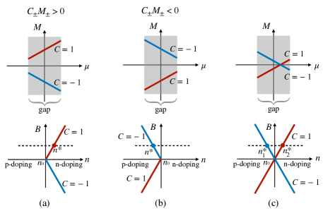
Figure 5: Chern insulator states can be identified by changes in the longitudinal resistivity at the density at which the gap opens. Using the Středa formula, a Chern insulator can be identified with extension of the $\nu=C$ Shubnikov-de Haas Landau fan feature to $B=0$. We note that positive magnetic fields favors states with positive magnetization. (a) The sign of $M$ does not change across the band gap and is the same as the sign of Hall conductivity. The anomalous quantum Hall state is more robust for $n$-doping because the Chern gap moves into the conduction band when a magnetic field is applied. (b) The sign of $M$ does not change across the band gap and is opposite to the sign of Hall conductivity. The anomalous quantum Hall state is then more robust for $p$-doping. (c) The sign of $M$ reverses across the band gap. The anomalous quantum Hall state is robust for both $n$- and $p$-doping, because the sign of the Chern number for a given magnetic field strength changes with carrier density.

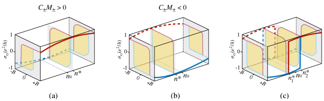
Figure 6: Schematic Hall conductivity hysteresis loops as sweeping the magnetic field at several carrier densities, and schematic Hall conductivity (solid and dashed lines) as a function of carrier density at magnetic fields on opposite extremes of the hysteresis loops. (a-b) Corresponding to Fig. 5(a-b) respectively, the Hall conductivity does not change sign when the system is tuned from $p$-doping to $n$-doping for a fixed magnetic field. (c) Corresponding to Fig. 5(c), the Hall conductivity changes sign when the system is tuned from $p$-doping to $n$-doping for a fixed magnetic field and is exactly quantized with opposite signs at two different densities $n_{1}^{*}$ and $n_{2}^{*}$.

References

- Chang et al. (2013) C.-Z. Chang, J. Zhang, X. Feng, J. Shen, Z. Zhang, M. Guo, K. Li, Y. Ou, P. Wei, L.-L. Wang, Z.-Q. Ji, Y. Feng, S. Ji, X. Chen, J. Jia, X. Dai, Z. Fang, S.-C. Zhang, K. He, Y. Wang, L. Lu, X.-C. Ma, and Q.-K. Xue, Science 340, 167 (2013).
- Sharpe et al. (2019) A. L. Sharpe, E. J. Fox, A. W. Barnard, J. Finney, K. Watanabe, T. Taniguchi, M. A. Kastner, and D. Goldhaber-Gordon, Science 365, 605 (2019).
- Chen et al. (a) G. Chen, A. L. Sharpe, E. J. Fox, Y.-H. Zhang, S. Wang, L. Jiang, B. Lyu, H. Li, K. Watanabe, T. Taniguchi, Z. Shi, T. Senthil, D. Goldhaber-Gordon, Y. Zhang, and F. Wang, (a), arXiv:1905.06535 .
- Serlin et al. (2019) M. Serlin, C. L. Tschirhart, H. Polshyn, Y. Zhang, J. Zhu, K. Watanabe, T. Taniguchi, L. Balents, and A. F. Young, Science (2019), 10.1126/science.aay5533.
- Polshyn et al. (a) H. Polshyn, J. Zhu, M. A. Kumar, Y. Zhang, F. Yang, C. L. Tschirhart, M. Serlin, K. Watanabe, T. Taniguchi, A. H. MacDonald, and A. F. Young, (a), arXiv:2004.11353 .
- Chen et al. (b) S. Chen, M. He, Y.-H. Zhang, V. Hsieh, Z. Fei, K. Watanabe, T. Taniguchi, D. H. Cobden, X. Xu, C. R. Dean, and M. Yankowitz, (b), arXiv:2004.11340 .
- Thouless et al. (1982) D. J. Thouless, M. Kohmoto, M. P. Nightingale, and M. den Nijs, Phys. Rev. Lett. 49, 405 (1982).
- Haldane (1988) F. D. M. Haldane, Phys. Rev. Lett. 61, 2015 (1988).
- Xiao et al. (2010) D. Xiao, M.-C. Chang, and Q. Niu, Rev. Mod. Phys. 82, 1959 (2010).
- (10) A. H. MacDonald, arXiv:cond-mat/9410047 .
- Bultinck et al. (2020) N. Bultinck, S. Chatterjee, and M. P. Zaletel, Phys. Rev. Lett. 124, 166601 (2020).
- Repellin et al. (2020) C. Repellin, Z. Dong, Y.-H. Zhang, and T. Senthil, Phys. Rev. Lett. 124, 187601 (2020).
- Zhang et al. (2019) Y.-H. Zhang, D. Mao, and T. Senthil, Phys. Rev. Research 1, 033126 (2019).
- Wu and Das Sarma (2020) F. Wu and S. Das Sarma, Phys. Rev. Lett. 124, 046403 (2020).
- (15) Y. Alavirad and J. D. Sau, arXiv:1907.13633 .
- (16) J. Liu and X. Dai, arXiv:1911.03760 .
- London (1948) F. London, Phys. Rev. 74, 562 (1948).
- Jung et al. (2015a) J. Jung, M. Polini, and A. H. MacDonald, Phys. Rev. B 91, 155423 (2015a).
- Po et al. (2019) H. C. Po, L. Zou, T. Senthil, and A. Vishwanath, Phys. Rev. B 99, 195455 (2019).
- Song et al. (2019) Z. Song, Z. Wang, W. Shi, G. Li, C. Fang, and B. A. Bernevig, Phys. Rev. Lett. 123, 036401 (2019).
- Lu et al. (2019) X. Lu, P. Stepanov, W. Yang, M. Xie, M. A. Aamir, I. Das, C. Urgell, K. Watanabe, T. Taniguchi, G. Zhang, A. Bachtold, A. H. MacDonald, and D. K. Efetov, Nature 574, 653 (2019).
- Bistritzer and MacDonald (2011) R. Bistritzer and A. H. MacDonald, Proceedings of the National Academy of Sciences 108, 12233 (2011).
- Thonhauser et al. (2005) T. Thonhauser, D. Ceresoli, D. Vanderbilt, and R. Resta, Phys. Rev. Lett. 95, 137205 (2005).
- Ceresoli et al. (2006) D. Ceresoli, T. Thonhauser, D. Vanderbilt, and R. Resta, Phys. Rev. B 74, 024408 (2006).
- Bianco and Resta (2013) R. Bianco and R. Resta, Phys. Rev. Lett. 110, 087202 (2013).
- Bianco and Resta (2016) R. Bianco and R. Resta, Phys. Rev. B 93, 174417 (2016).
- Wallbank et al. (2013) J. R. Wallbank, A. A. Patel, M. Mucha-Kruczyński, A. K. Geim, and V. I. Fal’ko, Phys. Rev. B 87, 245408 (2013).
- Moon and Koshino (2014) P. Moon and M. Koshino, Phys. Rev. B 90, 155406 (2014).
- Jung et al. (2015b) J. Jung, A. M. DaSilva, A. H. MacDonald, and S. Adam, Nature Communications 6, 6308 (2015b).
- Jung et al. (2017) J. Jung, E. Laksono, A. M. DaSilva, A. H. MacDonald, M. Mucha-Kruczyński, and S. Adam, Phys. Rev. B 96, 085442 (2017).
- Jung et al. (2014) J. Jung, A. Raoux, Z. Qiao, and A. H. MacDonald, Phys. Rev. B 89, 205414 (2014).
- Kindermann et al. (2012) M. Kindermann, B. Uchoa, and D. L. Miller, Phys. Rev. B 86, 115415 (2012).
- (33) J. Shi, J. Zhu, and A. H. MacDonald, in preparation (2020) .
- Rebeca et al. (2018) R.-P. Rebeca, C. Zhang, K. Watanabe, T. Taniguchi, J. Hone, and C. R. Dean, Science 361, 690 (2018).
- Hunt et al. (2013) B. Hunt, J. D. Sanchez-Yamagishi, A. F. Young, M. Yankowitz, B. J. LeRoy, K. Watanabe, T. Taniguchi, P. Moon, M. Koshino, P. Jarillo-Herrero, and R. C. Ashoori, Science 340, 1427 (2013).
- Finney et al. (2019) N. R. Finney, M. Yankowitz, L. Muraleetharan, K. Watanabe, T. Taniguchi, C. R. Dean, and J. Hone, Nature Nanotechnology 14, 1029 (2019).
- (37) Note that (dash-dotted line) should vanish when the flat bands are completely filled or completely empty because the total Chern number of all occupied bands is zero in both cases. The numerical error in Fig. 2(b) is difficult to be completely eliminated because small inaccuracies in the Berry curvature integrals are magnified when multiplied by a finite chemical potential .
- Xie and MacDonald (2020) M. Xie and A. H. MacDonald, Phys. Rev. Lett. 124, 097601 (2020).
- Checkelsky et al. (2014) J. G. Checkelsky, R. Yoshimi, A. Tsukazaki, K. S. Takahashi, Y. Kozuka, J. Falson, M. Kawasaki, and Y. Tokura, Nature Physics 10, 731 (2014).
- Kou et al. (2014) X. Kou, S.-T. Guo, Y. Fan, L. Pan, M. Lang, Y. Jiang, Q. Shao, T. Nie, K. Murata, J. Tang, Y. Wang, L. He, T.-K. Lee, W.-L. Lee, and K. L. Wang, Phys. Rev. Lett. 113, 137201 (2014).
- Bestwick et al. (2015) A. J. Bestwick, E. J. Fox, X. Kou, L. Pan, K. L. Wang, and D. Goldhaber-Gordon, Phys. Rev. Lett. 114, 187201 (2015).
- Chang et al. (2015) C.-Z. Chang, W. Zhao, D. Y. Kim, H. Zhang, B. A. Assaf, D. Heiman, S.-C. Zhang, C. Liu, M. H. W. Chan, and J. S. Moodera, Nature Materials 14, 473 (2015).
- Mogi et al. (2015) M. Mogi, R. Yoshimi, A. Tsukazaki, K. Yasuda, Y. Kozuka, K. S. Takahashi, M. Kawasaki, and Y. Tokura, Applied Physics Letters 107, 182401 (2015).
- (44) J. Jiang, D. Xiao, F. Wang, J.-H. Shin, D. Andreoli, J. Zhang, R. Xiao, Y.-F. Zhao, M. Kayyalha, L. Zhang, K. Wang, J. Zang, C. Liu, N. Samarth, M. H. W. Chan, and C.-Z. Chang, arXiv:1901.07611 .
- Dieny and Chshiev (2017) B. Dieny and M. Chshiev, Rev. Mod. Phys. 89, 025008 (2017).
- Streda (1982a) P. Streda, Journal of Physics C: Solid State Physics 15, L717 (1982a).
- (47) L. Wang, E.-M. Shih, A. Ghiotto, L. Xian, D. A. Rhodes, C. Tan, M. Claassen, D. M. Kennes, Y. Bai, B. Kim, K. Watanabe, T. Taniguchi, X. Zhu, J. Hone, A. Rubio, A. Pasupathy, and C. R. Dean, arXiv:1910.12147 .
- (48) P. Stepanov, I. Das, X. Lu, A. Fahimniya, K. Watanabe, T. Taniguchi, F. H. L. Koppens, J. Lischner, L. Levitov, and D. K. Efetov, arXiv:1911.09198 .
- Polshyn et al. (b) H. Polshyn, J. Zhu, M. A. Kumar, Y. Zhang, F. Yang, C. L. Tschirhart, M. Serlin, K. Watanabe, T. Taniguchi, A. H. MacDonald, and A. F. Young, (b), arXiv:2004.11353 .
- (50) Y. H. Kwan, Y. Hu, S. H. Simon, and S. A. Parameswaran, arXiv:2003.11560 .
- (51) A. Kumar, M. Xie, and A. H. MacDonald, in preparation (2020) .
- Holstein and Primakoff (1940) T. Holstein and H. Primakoff, Phys. Rev. 58, 1098 (1940).
- Mermin and Wagner (1966) N. D. Mermin and H. Wagner, Phys. Rev. Lett. 17, 1133 (1966).
- Kane and Mele (2005) C. L. Kane and E. J. Mele, Phys. Rev. Lett. 95, 226801 (2005).
- Min et al. (2006) H. Min, J. E. Hill, N. A. Sinitsyn, B. R. Sahu, L. Kleinman, and A. H. MacDonald, Phys. Rev. B 74, 165310 (2006).
- Yao et al. (2007) Y. Yao, F. Ye, X.-L. Qi, S.-C. Zhang, and Z. Fang, Phys. Rev. B 75, 041401 (2007).
- Konschuh et al. (2010) S. Konschuh, M. Gmitra, and J. Fabian, Phys. Rev. B 82, 245412 (2010).
- Boettger and Trickey (2007) J. C. Boettger and S. B. Trickey, Phys. Rev. B 75, 121402 (2007).
- Streda (1982b) P. Streda, Journal of Physics C: Solid State Physics 15, L1299 (1982b).