Large sample autocovariance matrices of linear processes with heavy tails

Abstract.

We provide asymptotic theory for certain functions of the sample autocovariance matrices of a high-dimensional time series with infinite fourth moment. The time series exhibits linear dependence across the coordinates and through time. Assuming that the dimension increases with the sample size, we provide theory for the eigenvectors of the sample autocovariance matrices and find explicit approximations of a simple structure, whose finite sample quality is illustrated for simulated data. We also obtain the limits of the normalized eigenvalues of functions of the sample autocovariance matrices in terms of cluster Poisson point processes. In turn, we derive the distributional limits of the largest eigenvalues and functionals acting on them. In our proofs, we use large deviation techniques for heavy-tailed processes, point process techniques motivated by extreme value theory, and related continuous mapping arguments.

1. Introduction

1.1. Some history

In time series analysis the notions of autocovariance, autocorrelation and their sample versions are basic tools for the study of the (linear) dependence structure, spectral analysis, parameter estimation, goodness-of-fit, change-point detection, etc.; see for example the classical monographs [7, 21]. When considering random matrices ${\mathbf{X}}={\mathbf{X}}_{n}=({\mathbf{x}}_{1},\ldots,{\mathbf{x}}_{n})$ with high-dimensional time series observations ${\mathbf{x}}_{t}=(X_{1t},\ldots,X_{pt})^{\prime}$, $t\in\mathbb{Z}$, the main focus of interest has been on the limiting spectral distribution of ${\mathbf{X}}$ and on the asymptotic properties of the eigenvalues and eigenvectors of the sample covariance matrix ${\mathbf{X}}{\mathbf{X}}^{\prime}$; see for instance [2]. From the observations $({\mathbf{x}}_{t})_{t\in\mathbb{Z}}$ one can also construct the $p\times n$ matrices

$${\mathbf{X}}_{n}(s)=({\mathbf{x}}_{1+s},\ldots,{\mathbf{x}}_{n+s})\,,\qquad s=0,1,2,\ldots\,,$$ (1.1)

while we refer to ${\mathbf{X}}={\mathbf{X}}_{n}(0)$ as the data matrix. Now, in analogy with the sample autocovariance function of a stationary process, we introduce the (non-normalized) sample autocovariance matrices at lag $s$:

$${\mathbf{X}}_{n}(0){\mathbf{X}}_{n}(s)^{\prime}\,,\qquad s=0,1,2,\ldots\,.$$ (1.2)

For $s=0$, we obtain the sample covariance matrix.

To the best of our knowledge, the idea of using functions of the sample autocovariance matrices originates from the paper [17]. The authors work in the framework of factor models for ${\mathbf{X}}$ and under light-tail assumptions on the entries $X_{it}$. The main goal of using sample autocovariance matrices in [17] was to derive a rule for determining a number of significant eigenvalues and eigenvectors for principal component analysis (PCA) in a high-dimensional time series setting. This was achieved by exploiting the additional information about the dependence of the time series $({\mathbf{x}}_{t})_{t\in\mathbb{Z}}$, contained in the sample autocovariance matrices ${\mathbf{X}}_{n}(0){\mathbf{X}}_{n}(s)^{\prime}$ for different lags $s\geq 0$.

Recently, a whole series of articles on sample autocovariance matrices was published. Again, factor models are assumed for describing the dynamics of the multivariate time series $({\mathbf{x}}_{t})_{t\in\mathbb{Z}}$. The authors of [19] study a ratio estimator for the number of relevant eigenvalues based on singular values of lagged sample autocovariance matrices. The paper proposes a complete theory of such sample singular values for both the factor and noise parts under the large-dimensional scheme where the dimension and the sample size grow proportionally to infinity. The papers [29, 30] consider a moment approach for determining the limiting spectral distribution of the singular values of the autocovariance matrices and for deriving the convergence of the largest singular value. The limiting spectral distribution of a symmetrized sample autocovariance matrix is studied in [15, 3, 20, 28] while [27] consider the extreme eigenvalues of such a matrix. The limiting spectral distribution of sample autocovariance matrices for factor models is investigated in [18].

1.2. Our model

In this paper we study the singular values of functions of the sample autocovariance matrices (1.2) at different lags $s$. Our model assumptions are quite distinct from most of the literature.

Growth condition on $p$

We describe high-dimensionality of the time series observations ${\mathbf{x}}_{t}=(X_{1t},\ldots,X_{pt})^{\prime}$ by assuming that $p=p_{n}\to\infty$ as $n\to\infty$. To be precise, we assume an integer sequence

$$p=p_{n}=n^{\beta}\ell(n),\quad n\geq 1, C_{p}(\beta)$$ ()

where $\ell$ is a slowly varying function and $\beta\in[0,1]$. This condition is more general than the growth conditions in the literature; see for example [16, 1, 26], where it is assumed that $p/n\to\gamma\in(0,\infty)$. Condition ($C_{p}(\beta)$) is also more general than in [9, 10] who have restrictions on the size of $\beta$, depending on the heaviness of the tails of ${\mathbf{X}}$.

Linear dependence

From a time series perspective it is natural to assume dependence between the entries $X_{it}$ both through time $t$ and across the rows $i$. In the aforementioned literature, dependence through time and across rows is often described by a factor model. This kind of model has been successfully used in econometrics.

We assume linear dependence between the rows and columns of ${\mathbf{X}}$:

$$X_{it}=\sum_{l\in\mathbb{Z}}\sum_{k\in\mathbb{Z}}h_{kl}\,Z_{i-k,t-l}\,,\qquad i,t\in\mathbb{Z}\,,$$ (1.3)

where $(Z_{it})_{i,t\in\mathbb{Z}}$ is an iid field of random variables with generic element $Z$ and $(h_{kl})_{k,l\in\mathbb{Z}}$ is a suitable array of real numbers such that the infinite series in (1.3) converges a.s.; see (1.5) below.

The model (1.3) was introduced in [10], assuming the rows iid, and, in the present form, used in [9, 8]. Linear dependence is a natural concept in time series analysis; it also allows one to describe the asymptotic properties of the eigenstructure of ${\mathbf{X}}{\mathbf{X}}^{\prime}$ in a transparent way.

Heavy-tail condition

In all the existing literature on sample autocovariance matrices it is assumed that the 4th moment of the entries $X_{it}$ is finite. We will refer to this condition as light tails. If 4th moments are infinite we instead refer to heavy tails. The reason for this distinction is that there is a phase transition in the limit behavior of the largest eigenvalues of the sample covariance matrix and, as we will see later, also of the largest singular values of the sample autocovariance matrices.

In the case of iid light-tailed $(X_{it})$ it is known that the largest eigenvalue of ${\mathbf{X}}{\mathbf{X}}^{\prime}$ typically has a Tracy-Widom limit distribution; see for example [16, 26] for benchmark results. This is in sharp contrast to the heavy-tail case. Due to work by [24, 25, 1] we know that the largest eigenvalue of the suitably normalized matrix ${\mathbf{X}}{\mathbf{X}}^{\prime}$ has a Fréchet limit distribution,

$$\Phi_{\alpha/2}(x)={\rm e}\,^{-x^{-\alpha/2}}\quad\mbox{for some $\alpha\in(0,4)$,}$$

which is one of the max-stable distributions, i.e., one of the limit distributions of normalized and centered maxima of an iid sequence, see [12, Chapter 3].

The assumption of infinite 4th moment is not sufficient to derive a precise weak limit theory for eigenvalues and singular values. Therefore, as in [25, 1, 14] in the iid case and in [10, 9, 8] in the linear dependence case we assume that $Z$ is regularly varying in the sense that the following tail balance condition holds

$$\mathbb{P}(Z>x)\sim p_{+}\dfrac{L(x)}{x^{\alpha}}\quad\mbox{and}\quad\mathbb{P}(Z<-x)\sim p_{-}\dfrac{L(x)}{x^{\alpha}}\,,\qquad x\to\infty\,,$$ (1.4)

for some tail index $\alpha\in(0,4)$, constants $p_{+},p_{-}\geq 0$ with $p_{+}+p_{-}=1$ and a slowly varying function $L$. The regular variation condition for $\alpha\in(0,4)$ implies that we consider the heavy-tail case where both $\mathbb{E}[Z^{4}]=\infty$ and $\mathbb{E}[X^{4}]=\infty$; see [8, 14, 13] for collections of results which show the stark differences between the heavy-tail and light-tail cases. In addition, we assume $\mathbb{E}[Z]=0$ whenever $\mathbb{E}[|Z|]<\infty$. Moreover, we also require the summability condition

$$\sum_{l\in\mathbb{Z}}\sum_{k\in\mathbb{Z}}|h_{kl}|^{\delta}<\infty\quad\mbox{for some $\delta\in(0,\min({\alpha/2},1))$.}$$ (1.5)

The conditions (1.4), (1.5) and $\mathbb{E}[Z]=0$ if $\mathbb{E}[|Z|]<\infty$ ensure the a.s. absolute convergence of the series in (1.3). Moreover, the marginal and finite-dimensional distributions of the field $(X_{it})$ are regularly varying with index $\alpha$; see for example [12], Appendix A3.3. Therefore we also refer to $(X_{it})$ and $(Z_{it})$ as regularly varying fields. Notice that regular variation of $(Z_{it})$ and the convergence of (1.3) imply that $(X_{it})$ constitutes a strictly stationary random field; we denote a generic element by $X$.

1.3. Functions of sample autocovariance matrices

Recall the definition of the sample autocovariance matrix at lag $s$ from (1.2). We are interested in the asymptotic behavior (of functions) of the eigen- and singular values of the matrices

$${\mathbf{C}}_{n}(s)=\left\{\begin{array}[]{ll}{\mathbf{X}}_{n}(0){\mathbf{X}}_{n}(s)^{\prime}\,,&\mbox{if }\alpha<2(1+\beta),\\ {\mathbf{X}}_{n}(0){\mathbf{X}}_{n}(s)^{\prime}-\mathbb{E}[{\mathbf{X}}_{n}(0){\mathbf{X}}_{n}(s)^{\prime}]\,,&\mbox{if }\alpha>2(1+\beta),\end{array}\right.\qquad s=0,1,2,\ldots.$$ (1.8)

For $\alpha>2(1+\beta)$, the centering $\mathbb{E}[{\mathbf{X}}_{n}(0){\mathbf{X}}_{n}(s)^{\prime}]$ is needed to ensure a non-degenerate limiting spectrum of ${\mathbf{C}}_{n}(s)$. A similar centering was used in [10, 9, 8]. The case $\alpha=2(1+\beta)$ is slightly more technical, but can be handled as well; see Remark 4.9 below.

The eigenvalues of the non-symmetric matrix ${\mathbf{C}}_{n}(s)$ for $s\geq 1$ can be complex. One way to avoid this is to calculate the singular values of this matrix, i.e., the square roots of the eigenvalues of the non-negative definite matrix ${\mathbf{C}}_{n}(s){\mathbf{C}}_{n}(s)^{\prime}$. The largest of these singular values is the spectral norm $\|{\mathbf{C}}_{n}(s)\|_{2}$.

In this paper, we study the asymptotic behavior of the eigenvalues and eigenvectors of the sum

$${\mathbf{P}}_{n}(s_{1},s_{2})=\sum_{s=s_{1}}^{s_{2}}{\mathbf{C}}_{n}(s){\mathbf{C}}_{n}(s)^{\prime}\quad\mbox{for fixed $0\leq s_{1}\leq s_{2}$.}$$ (1.9)

In what follows, we will often suppress the dependence of ${\mathbf{C}}_{n}$ and ${\mathbf{P}}_{n}$ on $n$ and simply write ${\mathbf{C}}$ and ${\mathbf{P}}$. This research is motivated by [17] who considered the ratio of successive largest eigenvalues of ${\mathbf{P}}_{n}(1,s)$ for various values $s\geq 1$. The goal was to find a value $s$ such that the relevant information about the eigenvalues contained in the sample autocovariances ${\mathbf{X}}_{n}(0){\mathbf{X}}_{n}(s)^{\prime}$ is exhausted.

1.4. Motivation and structure of this paper

When looking at the coordinates of the eigenvectors of sample autocovariance matrices of financial time series, we noticed that certain patterns, in particular around the largest coordinate values, occurred repetitively in several eigenvectors. Our goal was to find some theoretical explanation for this phenomenon. Another challenge was added by the stylized fact that financial time series are heavy-tailed. In contrast, most of the literature on dimension reduction and high-dimensional time series focuses on the light-tailed case.

We assume a linear dependence structure through time and across the rows for the underlying time series. The eigenvalues of large sample covariance matrices of linear processes was already studied in Davis et al. [10, 8, 9]. The sample autocovariance matrices call for additional challenges since they require to understand the interplay between the largest values of the noise $(Z_{it})$, the lag $s$ and the coefficient matrix $(h_{kl})$. We use large deviation theory for sums of heavy-tailed random variables in combination with point process convergence results and continuous mapping arguments to derive asymptotic theory for the eigenvectors and eigenvalues of large sample autocovariance matrices for time series with infinite fourth moment. Our results are very explicit as regards the dependence structure and magnitude of the largest eigenvalues as well as the construction of the corresponding eigenvectors.

This paper is organized as follows. Due to the complexity of the model the notation in this paper is rather involved. Therefore, in Section 2, we introduce the most important quantities used throughout the paper. In Section 3, we present the main asymptotic results. Theorem 3.1 provides explicit approximations to the eigenvalues of the matrix sum ${\mathbf{P}}_{n}(s_{1},s_{2})$. The major contribution of this work is the description of the eigenvectors of ${\mathbf{P}}_{n}(s_{1},s_{2})$. Theorem 3.3 contains explicit approximations of these eigenvectors under the additional restriction that the coefficient matrix $(h_{kl})$ has only finitely many non-zero entries. Extensions to coefficient matrices with infinitely many non-zero entries seem possible under an additional condition on the decay of $h_{kl}$ for $|k|\vee|l|\to\infty$. In Section 3.2 we also include detailed examples of our proposed eigenvector and eigenvalue approximations for simulated data and the S&P 500 log-returns. In Figures 2,4 and 5 the reader can convince him/herself with the naked eye that the eigenvectors possess the structure predicted by our asymptotic theory. Theorem 3.6 presents results on the weak convergence of the point process of the normalized eigenvalues of ${\mathbf{P}}_{n}(s_{1},s_{2})$ towards some cluster Poisson process. The limiting point process allows one to derive the asymptotic structure of the largest eigenvalues of ${\mathbf{P}}_{n}(s_{1},s_{2})$. Applications of the continuous mapping theorem yield asymptotic theory for functionals acting on the sequence of the eigenvalues such as the spectral gap, the ratio of the largest eigenvalue and the trace. In Section 3.4 we derive analogous results on the eigenstructure of sums of the symmetrized matrices $({\mathbf{C}}_{n}(s)+{\mathbf{C}}_{n}(s)^{\prime})/2$. Section 3.5 describes the limiting spectral distribution of the sample covariance matrix ${\mathbf{X}}{\mathbf{X}}^{\prime}$ when $p$ and $n$ are proportional. Section 4 contains the proofs of the main theorems.

2. More notation

Before we can formulate the main results we have to introduce relevant notation to be used throughout.

Order statistics

The order statistics of the field $(Z_{it}^{2})_{i=1,\ldots,p;t=1,\ldots,n}$

$$Z_{(1),np}^{2}\geq Z_{(2),np}^{2}\geq\cdots\geq Z_{(np),np}^{2},\qquad n,p\geq 1\,.$$ (2.1)

Sums of squares

$$D_{i}=D_{i}^{(n)}=\left\{\begin{array}[]{ll}\sum_{t=1}^{n}Z_{it}^{2}\,,&\mbox{if }\alpha<2(1+\beta),\\ \sum_{t=1}^{n}Z_{it}^{2}-n\mathbb{E}[Z^{2}]\,,&\mbox{if }\alpha>2(1+\beta),\end{array}\right.\qquad i=1,\ldots,p;\quad n\geq 1\,,$$ (2.4)

with generic element $D$ and their ordered squared values for fixed $n$,

$$D_{(1)}^{2}=D_{L_{1}}^{2}\geq\cdots\geq D_{(p)}^{2}=D_{L_{p}}^{2}\,.$$ (2.5)

We assume without loss of generality that $(L_{1},\ldots,L_{p})$ is a permutation of $(1,\ldots,p)$.

The matrices ${\mathbf{M}}(s)$ and ${\mathbf{K}}(s_{1},s_{2})$

We introduce some auxiliary matrices derived from the coefficients $(h_{kl})_{k,l\in\mathbb{Z}}$:

$${\mathbf{H}}(s)=(h_{k,l+s})_{k,l\in\mathbb{Z}},\qquad{\mathbf{M}}(s)={\mathbf{H}}(0){\mathbf{H}}(s)^{\prime}\,,\qquad s\geq 0\,.$$

Notice that

$$({\mathbf{M}}(s))_{ij}=\sum_{l\in\mathbb{Z}}h_{i,l}h_{j,l+s},\qquad i,j\in\mathbb{Z}.$$ (2.6)

For $0\leq s_{1}\leq s_{2}<\infty$, we define the positive semi-definite matrix

$${\mathbf{K}}(s_{1},s_{2})=\sum_{s=s_{1}}^{s_{2}}{\mathbf{M}}(s){\mathbf{M}}(s)^{\prime}$$ (2.7)

and denote its ordered eigenvalues by

$$v_{1}^{2}(s_{1},s_{2})\geq v_{2}^{2}(s_{1},s_{2})\geq\cdots\,.$$ (2.8)

We interpret $v_{i}(s_{1},s_{2})$ as the positive square root of $v_{i}^{2}(s_{1},s_{2})$.

Throughout this paper we assume that ${\mathbf{K}}(s_{1},s_{2})$ is not the null-matrix. Let $r(s_{1},s_{2})$ be the rank of ${\mathbf{K}}(s_{1},s_{2})$ so that $v_{r(s_{1},s_{2})}(s_{1},s_{2})>0$ while $v_{r(s_{1},s_{2})+1}(s_{1},s_{2})=0$ if $r(s_{1},s_{2})$ is finite, otherwise $v_{i}(s_{1},s_{2})>0$ for all $i$.

The singular values of ${\mathbf{M}}(s)$ are $(v_{i}(s,s))$; for ease of notation we will sometimes denote them by $(v_{i}(s))$. Under the summability condition (1.5) on $(h_{kl})$ for fixed $0\leq s_{1}\leq s_{2}<\infty$, denoting the Frobenius norm by $\|\cdot\|_{F}$,

$$\sum_{i=1}^{\infty}v_{i}^{2}(s_{1},s_{2}) = \sum_{s=s_{1}}^{s_{2}}\sum_{i=1}^{\infty}v_{i}^{2}(s)=\sum_{s=s_{1}}^{s_{2}}\|{\mathbf{M}}(s)\|_{F}^{2}=\sum_{s=s_{1}}^{s_{2}}\sum_{i,j\in\mathbb{Z}}\sum_{l_{1},l_{2}\in\mathbb{Z}}h_{i,l_{1}}h_{j,l_{1}+s}h_{i,l_{2}}h_{j,l_{2}+s}$$ (2.9)

$$\leq {\sum_{s=s_{1}}^{s_{2}}\Big{(}\sum_{l_{1},l_{2}\in\mathbb{Z}}\sum_{i\in\mathbb{Z}}|h_{i,l_{1}}h_{i,l_{2}}|\Big{)}^{2}}\leq c\,(s_{2}-s_{1})\sum_{l_{1}\in\mathbb{Z}}\sum_{i\in\mathbb{Z}}|h_{i,l_{1}}|<\infty\,.$$

Therefore all eigenvalues $v_{i}^{2}(s_{1},s_{2})$ are finite and the ordering (2.8) is justified.
Here and in what follows, we write $c$ for any positive constant whose value is not of interest.

Normalizing sequence

We define $(a_{k})$ by

$$\mathbb{P}(|Z|>a_{k})\sim k^{-1}\,,\qquad k\to\infty\,.$$

The largest eigenvalues of random matrices will typically be normalized by the sequence $(a_{np}^{4})$, where $p$ is given in ($C_{p}(\beta)$).

Eigenvalues of the sample autocovariance matrices

The ordered eigenvalues of ${\mathbf{P}}(s_{1},s_{2})$ in (1.9) are

$$\lambda_{1}(s_{1},s_{2})\geq\cdots\geq\lambda_{p}(s_{1},s_{2})\,,$$ (2.10)

where we suppress the dependence on $n$ in the notation.

Approximations to eigenvalues

Approximations to the ordered eigenvalues $\lambda_{i}(s_{1},s_{2})$ will be given in terms of the ordered values

$$\begin{array}[]{ll}\delta_{1}(s_{1},s_{2})\geq\cdots\geq\delta_{p}(s_{1},s_{2})&\mbox{from}\quad\big{\{}Z_{(i),np}^{4}v_{j}^{2}(s_{1},s_{2})\,,i=1,\ldots,p\,;j=1,2,\ldots\big{\}}\,,\\ \gamma_{1}(s_{1},s_{2})\geq\cdots\geq\gamma_{p}(s_{1},s_{2})&\mbox{from}\quad\big{\{}D_{i}^{2}v_{j}^{2}(s_{1},s_{2}),i=1,\ldots,p\,;j=1,2,\ldots\big{\}}\,.\end{array}$$ (2.13)

3. Approximations of eigenvalues and eigenvectors

In this section we provide the main approximation results for the ordered eigenvalues and the corresponding eigenvectors of the sample autocovariance matrices of the linear model (1.3). The relevant notation is given in Sections 1 and 2.

3.1. Eigenvalues of the sample autocovariance function

Theorem 3.1 (Eigenvalues of ${\mathbf{P}}(s_{1},s_{2})$).

Consider the linear process (1.3) under

• the growth condition ($C_{p}(\beta)$) on $(p_{n})$ for some $\beta\in[0,1]$,

• the regular variation condition (1.4) for some $\alpha\in(0,4)\backslash\{2(1+\beta)\}$,

• the centering condition $\mathbb{E}[Z]=0$ if $\mathbb{E}[|Z|]$ is finite,

• the summability condition (1.5) on the coefficient matrix $(h_{kl})$.

Then we have for $0\leq s_{1}\leq s_{2}<\infty$,

$$a_{np}^{-4}\max_{i=1,\ldots,p}|\lambda_{i}(s_{1},s_{2})-\gamma_{i}(s_{1},s_{2})|\stackrel{{\scriptstyle\mathbb{P}}}{{\rightarrow}}0,\quad n\to\infty.$$ (3.1)

Moreover, if $\alpha<2(1+\beta)$, then

$$a_{np}^{-4}\max_{i=1,\ldots,p}|\lambda_{i}(s_{1},s_{2})-\delta_{i}(s_{1},s_{2})|\stackrel{{\scriptstyle\mathbb{P}}}{{\rightarrow}}0,\quad n\to\infty.$$ (3.2)

The technical and quite lengthy proof of Theorem 3.1 can be found in Sections 4.3-4.5. For the convenience of the reader, we first present the main ideas of the proof in the setting of a filter $(h_{kl})$ with finitely many non-zero entries in Section 4.1.

The approximations (3.1) and (3.2) are strikingly simple considering the high dimension of ${\mathbf{P}}(s_{1},s_{2})$: apart from multiplication with the deterministic $(v_{j}^{2}(s_{1},s_{2}))$, the approximating values in Theorem 3.1 are just the order statistics of the iid sequences $(Z^{4}_{it})_{i\leq p;t\leq n}$ and $(D_{i}^{2})_{i\leq p}$, respectively.

Example 3.2.

We analyze a specific structure of the coefficients $h_{kl}$ of the linear process (1.3) and consider the separable case, i.e.,

$$h_{kl}=\left\{\begin{array}[]{ll}d_{k}\,c_{l}\,,&k,l\geq 0\,,\\ 0&\mbox{otherwise,}\end{array}\right.$$

for given real sequences ${\mathbf{d}}=(d_{0},d_{1},d_{2},\ldots)^{\prime}$ and ${\mathbf{c}}=(c_{0},c_{1},c_{2},\ldots)^{\prime}$, where we assume $d_{0}>0$ and that ${\mathbf{c}}$ is not the null sequence.

First, we determine the values $(\delta_{i}(s_{1},s_{2}))$ and $(\gamma_{i}(s_{1},s_{2}))$ which approximate the eigenvalues of the autocovariance function in Theorem 3.1. The matrix ${\mathbf{D}}={\mathbf{d}}{\mathbf{d}}^{\prime}$ is symmetric, has rank one and the only non-zero eigenvalue is $\overline{d}=\sum_{k=0}^{\infty}d_{k}^{2}$. We conclude from (2.6) that

$${\mathbf{M}}(s)=\overline{c}(s)\,{\mathbf{D}}\,,\qquad s\geq 0\,,$$ (3.4)

whose only non-zero eigenvalue is $\overline{d}\,\overline{c}(s)=\overline{d}\,\sum_{l=0}^{\infty}c_{l}c_{l+s}$. The factors $(\overline{c}(s))$ can be positive or negative; they constitute the autocovariance function of a stationary linear process $Y_{t}=\sum_{l=0}^{\infty}c_{l}\,V_{t-l}$, $t\in{\mathbb{Z}}$, where $(V_{i})$ is a unit variance white noise process.

From (2.7) and (3.4) we obtain for $0\leq s_{1}\leq s_{2}<\infty$ that

$${\mathbf{K}}(s_{1},s_{2})=\sum_{s=s_{1}}^{s_{2}}\overline{c}^{2}(s){\mathbf{D}}{\mathbf{D}}^{\prime}\,.$$ (3.5)

This matrix has rank $1$ and its largest eigenvalue is given by $v_{1}^{2}(s_{1},s_{2})=\sum_{s=s_{1}}^{s_{2}}\overline{c}^{2}(s)\,\,\overline{d}^{2}$. The approximating values in (3.1) and (3.2) are therefore

$$\gamma_{i}(s_{1},s_{2})=D_{(i)}^{2}\sum_{s=s_{1}}^{s_{2}}\overline{c}^{2}(s)\,\,\overline{d}^{2}\quad\text{ and }\quad\delta_{i}(s_{1},s_{2})=Z_{(i),np}^{4}\sum_{s=s_{1}}^{s_{2}}\overline{c}^{2}(s)\,\,\overline{d}^{2}\,,\quad 1\leq i\leq p\,.$$

Moreover, we have the remarkable identity

$$\gamma_{i}(s_{1},s_{2})=\sum_{s=s_{1}}^{s_{2}}\gamma_{i}(s,s)$$ (3.6)

which implies $\lambda_{i}(s_{1},s_{2})\approx\sum_{s=s_{1}}^{s_{2}}\lambda_{i}(s,s)$ for large $n$. For illustrations of this phenomenon on real and simulated data, see Figure 1 and the end of Example 3.4, respectively.

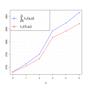
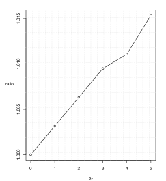
Figure 1. A comparison of the sums of the largest eigenvalues $\lambda_{1}(s,s)$ of the squared autocovariance matrices and the largest eigenvalue $\lambda_{1}(0,s_{2})$ of the sum of these matrices for $s_{2}=0,\ldots,5$. The underlying data ${\mathbf{X}}$ consists of $p=478$ log-return series composing the S&P 500 index estimated from $n=1345$ daily observations from 01/04/2010 to 02/28/2015. The two values are surprisingly close to each other; mind the scale of the $y$-axis. We also show the corresponding ratios which are very close to one.

3.2. Eigenvectors in the linear dependence model

In this section, $s_{1}\leq s_{2}$ are two given non-negative integers such that ${\mathbf{K}}(s_{1},s_{2})$ is not the null-matrix. The values $(s_{1},s_{2})$ are of no particular interest. Therefore we drop them in our notation. For example, we write ${\mathbf{K}}$, ${\mathbf{P}}$, $\lambda_{i}$ instead of ${\mathbf{K}}(s_{1},s_{2}),{\mathbf{P}}(s_{1},s_{2}),\lambda_{i}(s_{1},s_{2})$.

We provide approximations of the unit eigenvectors of ${\mathbf{P}}$ and give explicit expressions. For simplicity, we assume that $(h_{kl})$ is a matrix with finitely many non-zero entries. This means that $(X_{it})$ is a finite moving average both through time and across the rows.

Moreover, to solve identifyability issues of eigenvectors, we require that the eigenspace belonging to each non-zero eigenvalue of the deterministic matrix ${\mathbf{K}}$ is one-dimensional.

• Condition $H_{s_{1},s_{2}}$: (1) There exists an $m\in\mathbb{N}$ such that $h_{kl}=0$ if $|k|\vee|l|>m$.
  (2) There are no ties among the non-zero eigenvalues of ${\mathbf{K}}$ defined in (2.8).

Let ${\mathbf{y}}_{i}$ be the unit eigenvector of ${\mathbf{P}}$ associated with the non-zero eigenvalue $\lambda_{i}$, i.e., ${\mathbf{P}}{\mathbf{y}}_{i}=\lambda_{i}\,{\mathbf{y}}_{i}$ and $\|{\mathbf{y}}_{i}\|_{\ell_{2}}=1$. Throughout we use the convention that the first non-zero component of eigenvectors is assumed positive. Recall the definition of $\gamma_{i}$ from (2.13) and define the random indices $a(i),b(i)$ which satisfy the equation

$$\gamma_{i}=D_{a(i)}^{2}\,{v}_{b(i)}^{2}\,.$$

Under condition $H_{s_{1},s_{2}}$, the matrix ${\mathbf{K}}$ is zero outside of a block of size $(2m+1)\times(2m+1)$. More precisely, if we set $\widehat{\mathbf{K}}=({\mathbf{K}}_{i-m-1,j-m-1})_{i,j=1,\ldots,2m+1}$, then we have

$${\mathbf{K}}=\begin{pmatrix}\overline{\mathbf{0}}&&\\ &\widehat{\mathbf{K}}&\\ &&\overline{\mathbf{0}}\end{pmatrix}\,,$$ (3.7)

and the non-zero eigenvalues of $\widehat{\mathbf{K}}$ and ${\mathbf{K}}$ coincide. Here and in what follows, $\overline{\mathbf{0}}$ denotes a quadratic matrix consisting of zeros. We use this symbol to describe the structure of large matrices where the dimension of two $\overline{\mathbf{0}}$’s in the same line might be distinct or random.

By ${\mathbf{u}}_{i}=({\mathbf{u}}_{i,1},\ldots,{\mathbf{u}}_{i,2m+1})^{\prime}$ we denote the unit eigenvector of $\widehat{\mathbf{K}}$ associated with ${v}_{i}^{2}>0$, $i=1,\ldots,r={\rm{rank}}({\mathbf{K}})\leq 2m+1$. Under condition $H_{s_{1},s_{2}}$, the $({\mathbf{u}}_{i})$ are unique. We embed these $(2m+1)$-dimensional vectors into $p$-dimensional vectors ${\mathbf{u}}_{i}^{a}=({\mathbf{u}}_{i,1}^{a},\ldots,{\mathbf{u}}_{i,p}^{a})^{\prime}$, $a\in\mathbb{Z}$, via

$${\mathbf{u}}_{i,j}^{a}=\left\{\begin{array}[]{ll}{\mathbf{u}}_{i,j-a}\,,&j=(a-m)\vee 1,\ldots,(a+m)\wedge p\,,\\ 0\,,&\mbox{otherwise\,.}\end{array}\right.$$ (3.10)

The parameter $a$ encodes the location of ${\mathbf{u}}_{i}$ within ${\mathbf{u}}_{i}^{a}$. In other words,

$${\mathbf{u}}_{i}^{a}=(0,\ldots,0,{\mathbf{u}}_{i}^{\prime},0,\ldots,0)^{\prime}$$ (3.11)

and the location of zeros is determined by $a$.

Theorem 3.3 (Eigenvectors of ${\mathbf{P}}(s_{1},s_{2})$).

Assume the conditions of Theorem 3.1 and condition $H_{s_{1},s_{2}}$ with $0\leq s_{1}\leq s_{2}<\infty$. Then for $i\geq 1$,

$$\|{\mathbf{y}}_{i}(s_{1},s_{2})-{\mathbf{u}}_{b(i)}^{a(i)}(s_{1},s_{2})\|_{\ell_{2}}\stackrel{{\scriptstyle\mathbb{P}}}{{\rightarrow}}0\,,\qquad n\to\infty\,.$$

For $s_{1}=s_{2}=0$, Theorem 3.3 identifies the structure of the eigenvectors of the sample covariance matrix ${\mathbf{X}}{\mathbf{X}}^{\prime}$.

The proof of Theorem 3.3, which heavily relies on Section 4.1, is presented in Section 4.2.

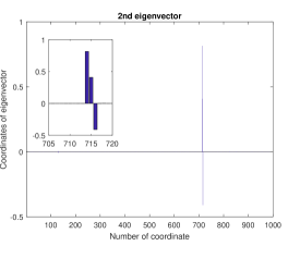
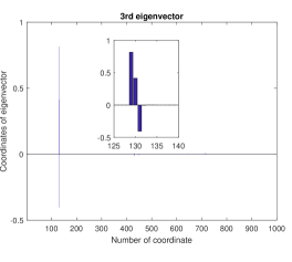
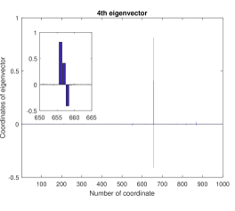
Figure 2. Coordinates of the four largest eigenvectors of ${\mathbf{P}}(0,0)$ in the separable case. The eigenvectors predicted by our model are of the form $6^{-1/2}\,(2,1,-1)^{\prime}$. After zooming in, it is easy to see that our approximation is very accurate. The eigenvectors of ${\mathbf{P}}(0,0),{\mathbf{P}}(1,1),{\mathbf{P}}(2,2)$; i.e., for lags 0,1,2; look exactly the same.

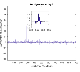
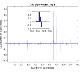
Figure 3. Coordinates of the leading eigenvectors of ${\mathbf{P}}(3,3)$ for underlying ${\mathbf{K}}(3,3)$-matrix being zero. The eigenvectors are very different from those of ${\mathbf{P}}(0,0),{\mathbf{P}}(1,1),{\mathbf{P}}(2,2)$; i.e., for lags 0,1,2.

Example 3.4.

We consider the separable case $h_{kl}=d_{k}c_{l}$ and re-use the setting of Example 3.2. In addition, we assume that $d_{k}=c_{k}=0$ for $k>m$.

Note that it is sufficient to focus on the non-zero elements of $\widehat{\mathbf{K}}$ in (3.7). By (3.5) and symmetry of ${\mathbf{D}}=(d_{i}d_{j})$, we obtain $\widehat{\mathbf{K}}(s_{1},s_{2})=\sum_{s=s_{1}}^{s_{2}}\overline{c}^{2}(s){\mathbf{D}}_{m}^{2}$, where ${\mathbf{D}}_{m}=(d_{i}d_{j})_{0\leq i,j\leq m}$. One easily checks that the $(m+1)$-dimensional unit eigenvector of ${\mathbf{D}}_{m}$ associated with its only non-zero eigenvalue $\overline{d}$ is

$${\mathbf{u}}_{1}=\overline{d}^{-1/2}(d_{0},\ldots,d_{m})^{\prime}\,.$$ (3.12)

By assumption $d_{0}>0$, this vector is oriented in accordance with our convention. Now we verify that ${\mathbf{u}}_{1}$ is also the eigenvector associated with the only non-zero eigenvalue $v_{1}^{2}(s_{1},s_{2})$ of $\widehat{\mathbf{K}}(s_{1},s_{2})$:

$$\sum_{s=s_{1}}^{s_{2}}\overline{c}^{2}(s){\mathbf{D}}_{m}^{2}\,{\mathbf{u}}_{1}=\sum_{s=s_{1}}^{s_{2}}\overline{c}^{2}(s)\overline{d}\,{\mathbf{D}}_{m}\,{\mathbf{u}}_{1}=v_{1}^{2}(s_{1},s_{2})\,{\mathbf{u}}_{1}\,.$$

By Theorem 3.3, for fixed $i$, the eigenvector ${\mathbf{y}}_{i}(s_{1},s_{2})$ is approximated by the $p$-dimensional vector that coincides with ${\mathbf{u}}_{1}$ at the $L_{i}$th to $(L_{i}+m)$th coordinates and has zero entries otherwise, i.e.,

$${\mathbf{u}}_{b(i)}^{a(i)}(s_{1},s_{2})={\mathbf{u}}_{1}^{L_{i}}(s_{1},s_{2})=(\underbrace{0,\ldots,0}_{L_{i}-1},{\mathbf{u}}_{1}^{\prime},0,\ldots,0)^{\prime}\,.$$ (3.13)

We illustrate the approximation of the leading eigenvectors by (3.13) in Figure 2. We set $(d_{0},d_{1},d_{2})=(2,1,-1)$ and $c_{0}=c_{1}=c_{2}=1$; all others are $0$. The iid field $(Z_{it})$ is simulated from a $t_{1.5}$ distribution. Then we construct the sample autocovariance matrices ${\mathbf{X}}_{n}(s)$, $s\geq 0$, for dimension $p=1000$ and sample size $n=10000$. From (3.12) one has

$${\mathbf{u}}_{1}=\dfrac{1}{\sqrt{6}}\,(2,1,-1)^{\prime}\,.$$ (3.14)

In Figure 2, we plot the 1000 coordinates of the $\ell_{2}$-normalized eigenvectors associated with the four largest eigenvalues of ${\mathbf{P}}(0,0)$. It is easy to see that these eigenvectors are of the form (3.13). Indeed, their coordinates are zero everywhere except some region which is determined by the location of the 4 largest values in the iid sequence $D_{1},\ldots,D_{p}$, that is $L_{1},\ldots,L_{4}$. The eigenvectors have a spike at $L_{i}$ of the form ${\mathbf{u}}_{1}$ which becomes apparent after zooming in around the $L_{i}$. In this example, the spikes appear at 3 coordinates since ${\mathbf{u}}_{1}$ is 3-dimensional. By choosing an appropriate sequence $(d_{0},\ldots,d_{m})$, it is possible to generate arbitrary spikes. The eigenvectors of ${\mathbf{P}}(1,1),{\mathbf{P}}(2,2),{\mathbf{P}}(0,2)$; i.e., for lags 1,2 and the sum of lags 0 to 2; look exactly the same as those of ${\mathbf{P}}(0,0)$. This phenomenon is due to independence of the approximate eigenvectors from $(s_{1},s_{2})$ in (3.13).

For the same data set we show, in Figure 3, the leading two eigenvectors of ${\mathbf{P}}(3,3)$, the squared sample autocovariance matrix at lag 3. Since ${\mathbf{K}}(3,3)$ is the null-matrix, the assumptions of Theorem 3.3 are violated. We observe that the structure of the plotted eigenvectors is very different from those in Figure 2 which correspond to non-null ${\mathbf{K}}$-matrices. Recall that the ${\mathbf{K}}$-matrix contains information about the largest entries of the sample autocovariance matrix. More precisely, it describes the entries with the heaviest tail index $\alpha/2$ which dominate the spectral behavior. If ${\mathbf{K}}$ is the null-matrix, it means that all autocovariance entries have the same tail index $\alpha$. Therefore the mass of the eigenvectors is more spread out what we observe in Figure 3. Moreover, it is interesting to note that, when zooming in around the largest coordinates of the eigenvectors, we see the somewhat familiar pattern of ${\mathbf{u}}_{1}$, though not as dominant as in Figure 2.

Next, we present some consequences of identity (3.6) for the sums of eigenvalues and the eigenvalues of sums of matrices. The following table contains the ratios of the largest eigenvalues of ${\mathbf{P}}(s,s)$ and ${\mathbf{P}}(0,0)$ for lags $s=1,\ldots,5$.

lag $s$	1	2	3	4	5
$\frac{\lambda_{1}(s,s)}{\lambda_{1}(0,0)}$	0.4444	0.1111	$3.31\cdot 10^{-6}$	$4.05\cdot 10^{-6}$	$7.43\cdot 10^{-6}$

The eigenvalue at lag 0 is of highest magnitude which can be explained by the inequality $|\overline{c}(s)|\leq\overline{c}(0)$. Our approximations for $\lambda_{1}(s,s)$, $s\geq 0$ in (3.1) are $\gamma_{1}(s,s)=D_{(1)}^{2}\overline{c}(s)^{2}\overline{d}^{2}$. In this example we have $\overline{c}(0)=3,\overline{c}(1)=2,\overline{c}(2)=1,\overline{c}(3)=0$. Hence,

$$\frac{\lambda_{1}(s,s)}{\lambda_{1}(0,0)}\approx\frac{\gamma_{1}(s,s)}{\gamma_{1}(0,0)}=\frac{\overline{c}(s)^{2}}{\overline{c}(0)^{2}}\,,$$

which provides a theoretical explanation for the values in the table. From lag 3 onwards, all the entries of the sample autocovariance matrix have lighter tails than some entries of the sample autocovariance matrices with smaller lags.

Finally, we calculate

$$\frac{\lambda_{1}(0,1)}{\lambda_{1}(0,0)}=1.4444\quad\text{ and }\quad\frac{\lambda_{1}(0,2)}{\lambda_{1}(0,0)}=1.5555\,.$$

In words, the sum of the largest eigenvalues of ${\mathbf{P}}(0,0)$ and ${\mathbf{P}}(1,1)$ equals the largest eigenvalue of $({\mathbf{P}}(0,0)+{\mathbf{P}}(1,1))$.

In Example 3.4, all non-null ${\mathbf{K}}(s_{1},s_{2})$-matrices had rank 1 and the same eigenvector ${\mathbf{u}}_{1}$ associated with $v_{1}^{2}(s_{1},s_{2})$. If the coefficients $(h_{kl})$ of the linear process (1.3) are such that ${\mathbf{K}}(s_{1},s_{2})$ has a rank higher than 1, and the eigenvectors depend on the lags $(s_{1},s_{2})$, one obtains a much richer structure of eigenvectors.

Example 3.5.

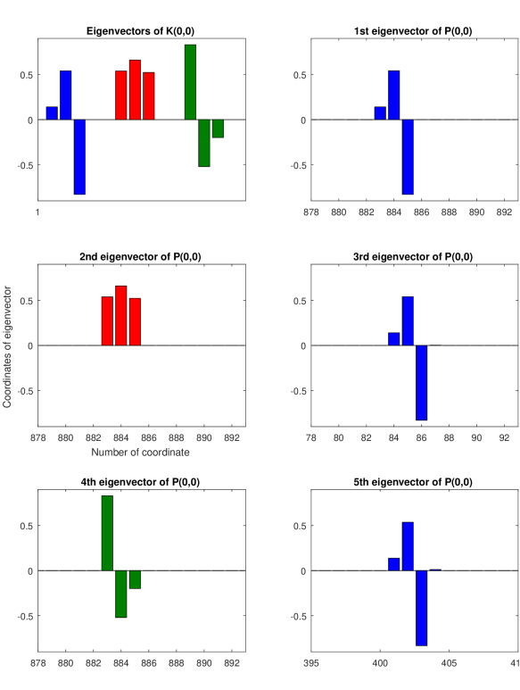
Figure 4. Eigenvectors of ${\mathbf{P}}(0,0)$ for a ${\mathbf{K}}$-matrix with rank 3.

We study the autocovariance matrices of the linear process (1.3), where $(Z_{it})$ is a field of independent identically $t$-distributed random variables with $1.5$ degrees of freedom. The coefficients of the linear process are given by

$$\begin{pmatrix}h_{00}&h_{01}&h_{02}\\ h_{10}&h_{11}&h_{12}\\ h_{20}&h_{21}&h_{22}\end{pmatrix}=\begin{pmatrix}1&2&0\\ 4&1&-1\\ -3&0&5\end{pmatrix}\,.$$ (3.15)

We work with simulated data $(X_{it})$ for dimension $p=1000$ and sample size $n=10000$. Our goal is to examine the quality of the asymptotic approximation of the $p$-dimensional eigenvectors of ${\mathbf{P}}(0,0)$ and ${\mathbf{P}}(1,1)$ provided by Theorem 3.3.

Since ${\mathbf{H}}$ is zero outside a $3\times 3$ block, the ${\mathbf{K}}$-matrices inherit this property by definition (2.7) and we will interpret them as $3\times 3$ matrices for simplicity.

We start with ${\mathbf{P}}(0,0)$. The eigenvalues of the deterministic ${\mathbf{K}}(0,0)$ are

$$v_{1}^{2}(0,0)=2080.1\,,\quad v_{2}^{2}(0,0)=89.1\,,\quad v_{3}^{2}(0,0)=3.8\,$$

with associated (normalized) eigenvectors

$${\mathbf{u}}_{1}(0,0)=\begin{pmatrix}0.1412\\ 0.5411\\ -0.8290\end{pmatrix}\,,\quad{\mathbf{u}}_{2}(0,0)=\begin{pmatrix}0.5392\\ 0.6602\\ 0.5228\end{pmatrix}\,,\quad{\mathbf{u}}_{3}(0,0)=\begin{pmatrix}0.8303\\ -0.5208\\ -0.1986\end{pmatrix}\,,$$

respectively. Recall that all vectors have Euclidean norm 1. The coordinates of ${\mathbf{u}}_{1}(0,0)$, ${\mathbf{u}}_{2}(0,0)$, ${\mathbf{u}}_{3}(0,0)$ are plotted in the top left panel of Figure 4 in blue, red and green, respectively. By Theorem 3.3 and (3.11), the eigenvectors of ${\mathbf{P}}(0,0)$ should resemble the appropriately shifted versions of ${\mathbf{u}}_{1}(0,0),{\mathbf{u}}_{2}(0,0),{\mathbf{u}}_{3}(0,0)$. Therefore we compute the eigenvectors of ${\mathbf{P}}(0,0)$ and try to match them with either a blue, red or green pattern from the top left panel.

The result for the eigenvectors associated with the 5 largest eigenvalues of ${\mathbf{P}}(0,0)$ is presented in Figure 4. The top right panel, for instance, shows the coordinates 878 to 893 of the first eigenvector. We zoomed in on the interesting region 878-893 since all other coordinates are very close to zero; compare also with Figure 2 where all coordinates and a zoom-in version are plotted. One immediately notices the pattern of ${\mathbf{u}}_{1}(0,0)$ at location $L_{1}=883$; see (2.5) for the definition of $L_{i}$. The color blue is chosen to emphasize the resemblance of the first eigenvector of ${\mathbf{P}}(0,0)$ to ${\mathbf{u}}_{1}(0,0)$.

In the second and third rows of Figure 2, we see that the blue, red and green patterns from the top left panel can be easily detected in the eigenvectors of ${\mathbf{P}}(0,0)$. Since ${\mathbf{K}}(0,0)$ has rank 3, we observe all 3 patterns.

The zoom-in location is determined by $(L_{i})$. In this example, the possible zoom-in locations are $L_{1},\ldots,L_{5}$. Moreover, it is possible to determine the $L_{i}$’s, which are defined in terms of order statistics of the iid noise, by looking at the eigenvector plots. From Figure 4 we can deduce the following: the pattern in the first eigenvector is always located at $L_{1}$ and therefore $L_{1}=883$. More generally, the largest $L_{i}$’s can be found by plotting the first, second, third,…eigenvectors of ${\mathbf{P}}(0,0)$. The $k$th appearance of the ${\mathbf{u}}_{1}(0,0)$ pattern corresponds to $L_{k}$. An inspection of the second column of Figure 4 gives $L_{1}=883,L_{2}=84$ and $L_{3}=401$; see also Figure 5.

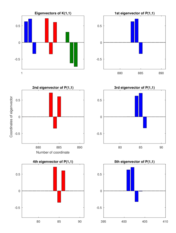
Figure 5. Eigenvectors of ${\mathbf{P}}(1,1)$ for a ${\mathbf{K}}$-matrix with rank 2.

In Figure 5 we show the leading eigenvectors of ${\mathbf{P}}(1,1)$. The eigenvalues of the deterministic ${\mathbf{K}}(1,1)$ are $v_{1}^{2}(1,1)=181.00,v_{2}^{2}(1,1)=66.99$ and $v_{3}^{2}(1,1)=0$ with associated (normalized) eigenvectors

$${\mathbf{u}}_{1}(1,1)=\begin{pmatrix}0.6242\\ 0.7050\\ -0.3368\end{pmatrix}\,,\quad{\mathbf{u}}_{2}(1,1)=\begin{pmatrix}0.7174\\ -0.3465\\ 0.6044\end{pmatrix}\,,\quad{\mathbf{u}}_{3}(1,1)=\begin{pmatrix}0.3094\\ -0.6189\\ -0.7220\end{pmatrix}\,,$$

respectively. The coordinates of ${\mathbf{u}}_{1}(1,1),{\mathbf{u}}_{2}(1,1),{\mathbf{u}}_{3}(1,1)$ are plotted in the top left panel of Figure 5 in blue, red and green, respectively. In contrast to ${\mathbf{K}}(0,0)$, the matrix ${\mathbf{K}}(1,1)$ does not have full rank. As a consequence the green pattern corresponding to ${\mathbf{u}}_{3}$ does not appear within the eigenvectors of ${\mathbf{P}}(1,1)$ (see Figure 5) and we only need to look for the the blue and red patterns. Indeed, in Theorem 3.3 only the eigenvectors ${\mathbf{u}}_{i}$ associated with positive eigenvalues of ${\mathbf{K}}$ are considered.

Next, we show the connection between the eigenvector plots and Theorem 3.1. To this end, recall that $\gamma_{i}(1,1)$ in (3.1) is the $i$th largest value in the set $\{v_{j}^{2}(1,1)D_{(\ell)}^{2}:j,\ell\geq 1\}$. The approximate eigenvectors in Theorem 3.3 are ${\mathbf{u}}_{b(i)(1,1)}^{a(i)(1,1)}(1,1)$, where $a(i)(1,1),b(i)(1,1)$ satisfy the equation $\gamma_{i}(1,1)=D_{a(i)(1,1)}^{2}\,{v}_{b(i)(1,1)}^{2}(1,1)$. The $b(i)$’s essentially decide which pattern will be observed in the sample autocovariance eigenvectors. In this example, we have $b(i)(1,1)\in\{1,2\}$. If $b(i)(1,1)=j$, we will see the ${\mathbf{u}}_{j}(1,1)$ pattern within the coordinates of the $i$th largest eigenvector of ${\mathbf{P}}(1,1)$. Consequently, the $b(i)$’s can be obtained from Figure 5. We immediately find

$$b(1)(1,1)=1,\quad b(2)(1,1)=2,\quad b(3)(1,1)=1,\quad b(4)(1,1)=2,\quad b(5)(1,1)=1\,.$$

Similarly, from Figure 4 we have

$$b(1)(0,0)=1,\quad b(2)(0,0)=2,\quad b(3)(0,0)=1,\quad b(4)(0,0)=3,\quad b(5)(0,0)=1\,.$$

To summarize, the eigenvector plots contain a lot of information about the model. The location of the spikes provides insight into the structure of the iid noise, while the spikes themselves can be viewed as functions of the $(h_{kl})$. More precisely, the vectors ${\mathbf{u}}_{i}(s_{1},s_{2})$ are functions of the coefficients $(h_{kl})$. If the number of non-zero coefficients is small, the ${\mathbf{u}}_{i}(s_{1},s_{2})$ can be estimated from the eigenvectors of ${\mathbf{P}}(s_{1},s_{2})$. Doing so for various pairs $(s_{1},s_{2})$, it is possible to invert the functional relation between ${\mathbf{u}}_{i}(s_{1},s_{2})$ and the coefficients. Hence, one can estimate the coefficients $(h_{kl})$ of the linear process.

While Example 3.5 treated the case of spikes of length 3, one easily obtains spikes of length $m$ by replacing (3.15) by a matrix with $m$ rows. The computational effort would stay the same provided $m$ is small relative to the dimension $p$. This setting is quite natural for factor models.

3.3. Point process convergence

Theorem 3.1 and arguments similar to the proofs in [8] enable one to derive the weak convergence of the point processes of the normalized eigenvalues of ${\mathbf{P}}(s_{1},s_{2})$:

$$N_{n}^{(s_{1},s_{2})}=\sum_{i=1}^{p}\delta_{a_{np}^{-4}\lambda_{i}(s_{1},s_{2})}\,,$$ (3.16)

where $\delta_{x}$ denotes the Dirac measure at $x$.

Theorem 3.6.

Assume the conditions of Theorem 3.1. Then $(N_{n}^{(s_{1},s_{2})})$ converge weakly in the space of point measures with state space $(0,\infty)$ equipped with the vague topology:

$$N_{n}^{(s_{1},s_{2})}\stackrel{{\scriptstyle d}}{{\rightarrow}}N^{(s_{1},s_{2})}=\sum_{i=1}^{\infty}\sum_{j=1}^{\infty}\delta_{\Gamma_{i}^{-4/\alpha}v_{j}^{2}(s_{1},s_{2})}\,,\qquad n\to\infty.$$ (3.17)

Here

$$\Gamma_{i}=E_{1}+\cdots+E_{i}\,,\qquad i\geq 1\,,$$

and $(E_{i})$ is an iid standard exponential sequence.

For the proof of Theorem 3.6 one can follow the lines of the proof of Theorem 3.4 in [8]; we omit further details.

Remark 3.7.

Since (3.17) is based on a continuous mapping argument involving the same points $\Gamma_{i}^{-4/\alpha}$ for arbitrary $(s_{1},s_{2})$, (3.17) immediately extends to processes whose multivariate points consist of $a_{np}^{-4}\lambda_{i}(s_{1},s_{2})$ for distinct choices of $(s_{1},s_{2})$.

The limiting point process in (3.17) yields a plethora of ancillary results. For example, one can easily derive the limiting distribution of $a_{np}^{-4}\lambda_{k}(s_{1},s_{2})$ for fixed $k\geq 1$:

$$\begin{split}\lim_{n\to\infty}\mathbb{P}(a_{np}^{-4}\lambda_{k}(s_{1},s_{2})\leq x)&=\lim_{n\to\infty}\mathbb{P}(N_{n}^{(s_{1},s_{2})}(x,\infty)<k)=\mathbb{P}(N^{(s_{1},s_{2})}(x,\infty)<k)\,,\quad x>0\,.\end{split}$$

In particular,the normalized largest eigenvalue has a re-scaled $\Phi_{\alpha/4}$-Fréchet distribution:

$$\begin{split}\lim_{n\to\infty}\mathbb{P}(a_{np}^{-4}\lambda_{1}(s_{1},s_{2})\leq x)&=\mathbb{P}(\Gamma_{1}^{-4/\alpha}v_{1}^{2}(s_{1},s_{2})\leq x)=\exp(-x^{-\alpha/4}v_{1}^{\alpha/2}(s_{1},s_{2})),\quad x>0\,.\end{split}$$

In the paper [17] the following estimator was considered in the context of a factor model for $s_{1}=1$, and fixed values $s_{2},k\geq 1$:

$$\underset{1\leq i\leq k}{\mathrm{arg\,min}}\,\dfrac{\lambda_{i+1}(s_{1},s_{2})}{\lambda_{i}(s_{1},s_{2})}\,.$$ (3.18)

Writing $q_{i}$ for the $i$th largest value in the set $\{v_{j}^{2}(s_{1},s_{2})\Gamma_{\ell}^{-4/\alpha}:j,\ell\geq 1\}$, we have the joint convergence of the ratios

$$\Big{(}\dfrac{\lambda_{2}(s_{1},s_{2})}{\lambda_{1}(s_{1},s_{2})},\ldots,\dfrac{\lambda_{k+1}(s_{1},s_{2})}{\lambda_{k}(s_{1},s_{2})}\Big{)}\stackrel{{\scriptstyle\rm d}}{{\rightarrow}}\Big{(}\dfrac{q_{2}}{q_{1}},\ldots,\dfrac{q_{k+1}}{q_{k}}\Big{)}\,.$$ (3.19)

Hence the limit distribution for the estimator (3.18) can be achieved by simulation.

In particular, if $r(s_{1},s_{2})=1$, another immediate consequence of (3.17) is

$$\frac{\big{(}\lambda_{1}(s_{1},s_{2}),\ldots,\lambda_{k+1}(s_{1},s_{2})\big{)}}{a_{np}^{4}\,v_{1}^{2}(s_{1},s_{2})}\stackrel{{\scriptstyle\rm d}}{{\rightarrow}}\big{(}\Gamma_{1}^{-4/\alpha},\ldots,\Gamma_{k+1}^{-4/\alpha}\big{)}\,,$$

so that (3.19) reads as

$$\Big{(}\dfrac{\lambda_{2}(s_{1},s_{2})}{\lambda_{1}(s_{1},s_{2})},\ldots,\dfrac{\lambda_{k+1}(s_{1},s_{2})}{\lambda_{k}(s_{1},s_{2})}\Big{)}\stackrel{{\scriptstyle\rm d}}{{\rightarrow}}\Big{(}\Big{(}\dfrac{\Gamma_{1}}{\Gamma_{2}}\Big{)}^{4/\alpha},\ldots,\Big{(}\dfrac{\Gamma_{k}}{\Gamma_{k+1}}\Big{)}^{4/\alpha}\Big{)}\,.$$

Hence the limit distribution would not depend on $(s_{1},s_{2})$ in this case. Notice that the ratios $\Gamma_{i}/\Gamma_{i+1}$ are independent Beta$(i,1)$-distributed for $i=1,\ldots,k$. Therefore

$$-\Big{(}\log\dfrac{\lambda_{2}(s_{1},s_{2})}{\lambda_{1}(s_{1},s_{2})},2\,\log\dfrac{\lambda_{3}(s_{1},s_{2})}{\lambda_{2}(s_{1},s_{2})},\ldots,k\,\log\dfrac{\lambda_{k+1}(s_{1},s_{2})}{\lambda_{k}(s_{1},s_{2})}\Big{)}\stackrel{{\scriptstyle\rm d}}{{\rightarrow}}\dfrac{4}{\alpha}\,(E_{1},\ldots,E_{k})\,.$$

A continuous mapping argument similar to [22], Theorem 7.1, yields for the trace

$$a_{np}^{-4}\,{\rm tr}\big{(}{\mathbf{P}}(s_{1},s_{2})\big{)}=a_{np}^{-4}\sum_{i=1}^{p}\lambda_{i}(s_{1},s_{2})\stackrel{{\scriptstyle\rm d}}{{\rightarrow}}\sum_{j=1}^{\infty}v_{j}^{2}(s_{1},s_{2})\sum_{i=1}^{\infty}\Gamma_{i}^{-4/\alpha}\,.$$

Since $\alpha\in(0,4)$, the right-hand series converges a.s. and represents a positive $\alpha/4$-stable random variable; see [23] for more information on series representations of stable random variables. We also have the joint convergence

$$a_{np}^{-4}\Big{(}\lambda_{1}(s_{1},s_{2})\,,{\rm tr}\big{(}{\mathbf{P}}(s_{1},s_{2})\big{)}\Big{)}\stackrel{{\scriptstyle\rm d}}{{\rightarrow}}\Big{(}v_{1}^{2}(s_{1},s_{2})\Gamma_{1}^{-4/\alpha},\sum_{j=1}^{\infty}v_{j}^{2}(s_{1},s_{2})\sum_{i=1}^{\infty}\Gamma_{i}^{-4/\alpha}\Big{)}\,.$$

Therefore we have self-normalized convergence of the largest eigenvalue $\lambda_{1}(s_{1},s_{2})$

$$\dfrac{\lambda_{1}(s_{1},s_{2})}{{\rm tr}\big{(}{\mathbf{P}}(s_{1},s_{2})\big{)}}\stackrel{{\scriptstyle\rm d}}{{\rightarrow}}\dfrac{v_{1}^{2}(s_{1},s_{2})}{\sum_{j=1}^{\infty}v_{j}^{2}(s_{1},s_{2})}\dfrac{\Gamma_{1}^{-4/\alpha}}{\sum_{i=1}^{\infty}\Gamma_{i}^{-4/\alpha}}\,.$$

The limiting variable is the scaled quotient of a $\Phi_{\alpha/4}$-Fréchet random variable and a positive $\alpha/4$-stable random variable.

3.4. Singular values of the symmetrization

For $s\geq 1$, the sample autocovariance matrix ${\mathbf{C}}(s)$ may have complex eigenvalues. An alternative way of creating real eigenvalues is by applying symmetrization. Therefore we study the matrix

$${\mathbf{A}}_{n}(s_{1},s_{2})=\sum_{s=s_{1}}^{s_{2}}\mbox{$\frac{1}{2}$}\,\big{(}{\mathbf{C}}_{n}(s)+{\mathbf{C}}_{n}(s)^{\prime}\big{)}\,$$ (3.20)

and its singular values

$$\sigma_{1}(s_{1},s_{2})\geq\cdots\geq\sigma_{p}(s_{1},s_{2})\geq 0\,.$$

Our focus is on singular values because the eigenvalues can be negative. This corresponds to an ordering of eigenvalues with respect to their absolute values.

The role of the matrix ${\mathbf{K}}(s_{1},s_{2})$ in (2.7) will now be played by

$$\widetilde{\mathbf{K}}(s_{1},s_{2})=\sum_{s=s_{1}}^{s_{2}}\mbox{$\frac{1}{2}$}\,\big{(}{\mathbf{M}}(s)+{\mathbf{M}}(s)^{\prime}\big{)}$$ (3.21)

with ordered singular values $\widetilde{v}_{1}(s_{1},s_{2})\geq\widetilde{v}_{2}(s_{1},s_{2})\geq\cdots$. Again we assume that $\widetilde{\mathbf{K}}(s_{1},s_{2})$ is not the null-matrix. Then we have the following analog of Theorem 3.1.

Theorem 3.8.

Assume the conditions of Theorem 3.1. Then we have for $0\leq s_{1}\leq s_{2}<\infty$,

$$a_{np}^{-4}\max_{i=1,\ldots,p}|\sigma_{i}(s_{1},s_{2})-\widetilde{\gamma}_{i}(s_{1},s_{2})|\stackrel{{\scriptstyle\mathbb{P}}}{{\rightarrow}}0,\quad n\to\infty\,,$$ (3.22)

where $(\widetilde{\gamma}_{i}(s_{1},s_{2}))$ are the ordered values of the set $\big{\{}D_{(i)}\widetilde{v}_{j}(s_{1},s_{2})\,,i=1,\ldots,p\,;j=1,2,\ldots\big{\}}$.

Moreover, if $\alpha<2(1+\beta)$, then

$$a_{np}^{-4}\max_{i=1,\ldots,p}|\sigma_{i}(s_{1},s_{2})-\widetilde{\delta}_{i}(s_{1},s_{2})|\stackrel{{\scriptstyle\mathbb{P}}}{{\rightarrow}}0,\quad n\to\infty\,,$$

where $(\widetilde{\delta}_{i}(s_{1},s_{2}))$ are the ordered values of the set $\big{\{}Z_{(i),np}^{2}\widetilde{v}_{j}(s_{1},s_{2})\,,i=1,\ldots,p\,;j=1,2,\ldots\big{\}}$.

An inspection of the proof of Theorem 3.1 shows that all its parts can be modified when ${\mathbf{P}}_{n}(s_{1},s_{2})$ is replaced by ${\mathbf{A}}_{n}(s_{1},s_{2})$; therefore we omit a proof. Theorem 3.3 also remains valid for the eigenvectors ${\mathbf{y}}_{i}(s_{1},s_{2})$ of ${\mathbf{A}}_{n}(s_{1},s_{2})$ if we let the ${\mathbf{u}}_{i}(s_{1},s_{2})$ denote the eigenvectors of $\widetilde{\mathbf{K}}(s_{1},s_{2})$.

As an analog of Theorem 3.6 we get

$$\sum_{i=1}^{p}\delta_{a_{np}^{-2}\sigma_{i}(s_{1},s_{2})}\stackrel{{\scriptstyle d}}{{\rightarrow}}\sum_{i=1}^{\infty}\sum_{j=1}^{\infty}\delta_{\Gamma_{i}^{-2/\alpha}\widetilde{v}_{j}(s_{1},s_{2})}\,,\qquad n\to\infty.$$

Example 3.9.

Again, we consider the separable case and use the notation and assumptions from Examples 3.2 and 3.4.

By symmetry of ${\mathbf{D}}$, we find

$$\widetilde{\mathbf{K}}(s_{1},s_{2})=\sum_{s=s_{1}}^{s_{2}}\mbox{$\frac{1}{2}$}\,\big{(}{\mathbf{M}}(s)+{\mathbf{M}}(s)^{\prime}\big{)}=\sum_{s=s_{1}}^{s_{2}}\overline{c}(s){\mathbf{D}}\,.$$

The approximating values in (3.22) are therefore $\widetilde{\gamma}_{i}(s_{1},s_{2})=D_{(i)}|\sum_{s=s_{1}}^{s_{2}}\overline{c}(s)|\,\,\overline{d}$, $1\leq i\leq p$. In contrast to the equality (3.6), we only obtain the inequality

$$\widetilde{\gamma}_{i}(s_{1},s_{2})\leq\sum_{s=s_{1}}^{s_{2}}\widetilde{\gamma}_{i}(s,s)\,$$ (3.23)

for the symmetrized autocovariances. This is due to the fact that $\overline{c}(s)$ can be positive or negative. Different signs lead to a cancellation effect which reduces the magnitude of the singular values.

Since $|\overline{c}(s)|\leq\overline{c}(0)$ for $s>1$ we also observe that the approximating quantities $\widetilde{\gamma}_{i}(s,s)$ are always dominated by $\widetilde{\gamma}_{i}(0,0)$. Using that $(\overline{c}(s))$ is a non-negative definite function, we conclude that $\sum_{s=0}^{s_{0}}\overline{c}(s)\geq 0$, hinting at the fact that lag $0$ is of central importance.

Finally, if the ${\mathbf{c}}$-sequence has non-negative components, then there is equality in (3.23) which implies $\widetilde{\sigma}_{i}(s_{1},s_{2})\approx\sum_{s=s_{1}}^{s_{2}}\widetilde{\sigma}(s,s)$ for large $n$. It is apparent in Figure 6(b) that this approximation does not necessarily hold for real-life return data.

An approximation to the eigenvector of ${\mathbf{A}}_{n}(s_{1},s_{2})$ associated with the $i$th largest absolute eigenvalue is given by (3.13).

As regards point processes, we have

$$\sum_{i=1}^{p}\delta_{a_{np}^{-2}\,\widetilde{v}_{1}^{-1}(s_{1},s_{2})\,\sigma_{i}(s_{1},s_{2})}\stackrel{{\scriptstyle\rm d}}{{\rightarrow}}\sum_{i=1}^{\infty}\delta_{\Gamma_{i}^{-2/\alpha}}\,,\qquad n\to\infty\,.$$

In other words, the limit is a Poisson point process on $(0,\infty)$ with mean measure $\mu(x,\infty)=x^{-\alpha/2}$, $x>0$.

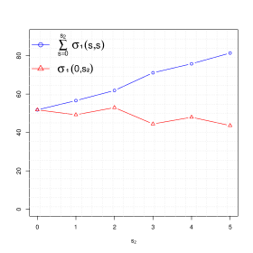
Figure 6. (a): A comparison of the sums of the largest eigenvalues $\lambda_{1}(s,s)$ of the squared sample autocovariance matrices and the largest eigenvalue $\lambda_{1}(0,s_{2})$ of the sum of these matrices for $s_{2}=0,\ldots,5$. The underlying data ${\mathbf{X}}$ consists of $p=478$ log-return series composing the S&P 500 index estimated from $n=1345$ daily observations from 01/04/2010 to 02/28/2015. (b): We compare the sum of the largest largest singular values of the symmetrized sample autocovariance matrices and the largest singular value of their sum. The matrices in the latter sum might not be positive definite which is a possible explanation for the observed cancellation effect.

3.5. Limiting spectral distribution

So far we studied the behaviors of the largest eigenvalues of sample autocovariance matrices. In Section 3.3, we employed point process techniques to describe their joint convergence. We saw that they are separated from each other, which in turn enabled us to characterize the associated eigenvectors in Section 3.2. In contrast, the bulk (or non-extreme) eigenvalues are usually not separated. The bulk is often studied via the so–called empirical spectral distribution which is defined for a $p\times p$ matrix ${\mathbf{A}}$ with real eigenvalues $\lambda_{1}({\mathbf{A}}),\ldots,\lambda_{p}({\mathbf{A}})$ by

$$F_{{\mathbf{A}}}(x)=\frac{1}{p}\;\sum_{i=1}^{p}\mathbf{1}_{\{\lambda_{i}({\mathbf{A}})\leq x\}},\qquad x\in\mathbb{R}\,.$$

The empirical spectral distribution is uniquely characterized by its Stieltjes transform

$$s_{{\mathbf{A}}}(z)=\int_{\mathbb{R}}\frac{1}{x-z}\,\mathrm{d}F_{{\mathbf{A}}}(x)\,,\quad z\in\mathbb{C}^{+}\,,$$

where $\mathbb{C}^{+}$ denotes the complex numbers with positive imaginary part; see for instance [31].

In this subsection, we describe the limit of the empirical spectral distributions of the sample covariance matrices when $p$ and $n$ grow proportionally. An application of Corollary 7 in [4] yields the following result.

Proposition 3.10.

Consider the linear process (1.3) and assume that

• $p/n\to\gamma\in(0,\infty)$,

• $\mathbb{E}[Z^{2}]=1$ and $\mathbb{E}[Z]=0$,

• the summability condition $\sum_{k,l\in\mathbb{Z}}|h_{kl}|<\infty$ holds.

Then the empirical spectral distributions $F_{n^{-1}{\mathbf{X}}{\mathbf{X}}^{\prime}}$ converge, with probability 1, to a nonrandom distribution function $F$ whose Stieltjes transform $s$ satisfies

$$s(z)=\int_{0}^{1}h(x,z)\,\mathrm{d}x\,,\quad z\in\mathbb{C}^{+}\,,$$ (3.24)

where $h(x,z)$ is a solution to the equation

$$h(x,z)=\Big{(}-z+\int_{0}^{1}\frac{f(x,t)}{1+\gamma\int_{0}^{1}f(u,t)h(u,z)\,\mathrm{d}u}\,\mathrm{d}t\Big{)}^{-1}$$

with

$$f(x,y)=\sum_{k,l\in\mathbb{Z}}\gamma_{kl}\operatorname{e}^{-2\pi\mathbf{i}(kx+ly)}\quad\text{ and }\quad\gamma_{kl}=\sum_{u,v\in\mathbb{Z}}h_{uv}h_{u-k,v-l}\,.$$

The distribution function $F$ can be obtained numerically from (3.24); we refer to [11] for details. In the iid case, i.e. $X_{it}=Z_{it}$, (3.24) reads as $s(z)=\frac{1+\gamma s(z)}{-z-z\gamma zs(z)+1}$ with solution

$$s_{F_{\gamma}}(z)=\frac{1-\gamma-z+\sqrt{(1+\gamma-z)^{2}-4\gamma}}{2\gamma z}\,,\quad z\in\mathbb{C}^{+}\,.$$ (3.25)

This is the Stieltjes transform of the famous Marčenko–Pastur law $F_{\gamma}$. If $\gamma\in(0,1]$, $F_{\gamma}$ has density,

$$f_{\gamma}(x)=\left\{\begin{array}[]{ll}\frac{1}{2\pi x\gamma}\sqrt{(b-x)(x-a)}\,,&\mbox{if }a\leq x\leq b,\\ 0\,,&\mbox{otherwise,}\end{array}\right.$$ (3.28)

where $a=(1-\sqrt{\gamma})^{2}$ and $b=(1+\sqrt{\gamma})^{2}$. If $\gamma>1$, the Marčenko–Pastur law has an additional point mass $1-1/\gamma$ at $0$.

Remark 3.11.

There is a minor typo in Corollary 7 of [4]. In the definition of $\mathbb{B}_{N}$, $N^{-1}$ needs to be replaced by $p^{-1}$; compare with equation (11) of the same paper.

4. Proofs

4.1. Sketch of the proof of Theorem 3.1 in the case of a finite filter

We consider a finite filter $(h_{kl})$ in the sense that for some $m\in\mathbb{N}$ we have $h_{kl}=0$ if $|k|\vee|l|>m$. This implies that ${\mathbf{M}}(s)_{ij}=0$ for $|i|\vee|j|>m$ and all $s\geq 0$. In words, ${\mathbf{M}}(s)$ is zero outside of a block of size $(2m+1)\times(2m+1)$. Now we embed this block into $p\times p$ matrices ${\mathbf{M}}_{a}(s)=({\mathbf{M}}_{a}(s)_{ij})_{i,j=1,\ldots,p}$, $a\in\mathbb{Z}$, which we define by

$${{\mathbf{M}}}_{a}(s)_{ij}=\left\{\begin{array}[]{ll}{{\mathbf{M}}}(s)_{i-a,j-a}\,,&i,j=(a-m)\vee 1,\ldots,(a+m)\wedge p\,,\\ 0\,,&\mbox{otherwise.}\end{array}\right.$$ (4.3)

For $m+1\leq a\leq p-m$, ${{\mathbf{M}}}(s)$ has the following block-diagonal form

$${\mathbf{M}}(s)=\begin{pmatrix}\overline{\mathbf{0}}&&\\ &{\mathbf{M}}_{a}(s)&\\ &&\overline{\mathbf{0}}\end{pmatrix}\,.$$

Recall that $\overline{\mathbf{0}}$ denotes a quadratic matrix consisting of zeros.

By Theorem 4.2 below, we have for any integer sequence $k=k_{p}\to\infty$ such that $k_{p}^{2}=o(p)$,

$$a_{np}^{-2}\Big{\|}{\mathbf{C}}_{n}(s)-\sum_{i=1}^{k}D_{(i)}{\mathbf{M}}_{L_{i}}(s)\Big{\|}_{2}\stackrel{{\scriptstyle\mathbb{P}}}{{\rightarrow}}0\,,\quad n\to\infty\,.$$ (4.4)

For such a $k$ it holds $\mathbb{P}(A_{n})\to 1$, where

$$A_{n}=\{|L_{i}-L_{j}|>2m+1\,,i,j=1,\ldots,k\,,i\neq j\}\cap\{1\leq L_{i}-m\leq L_{i}+m\leq p\,,i=1,\ldots,k\}\,.$$ (4.5)

On the set $A_{n}$, we have

$${\mathbf{M}}_{L_{i}}(s){\mathbf{M}}_{L_{j}}(s)^{\prime}=\overline{\mathbf{0}}\,,\quad i,j=1,\ldots,k\,,i\neq j\,.$$ (4.6)

A combination of (4.4) and (4.6) shows

$$a_{np}^{-4}\Big{\|}{\mathbf{P}}(s_{1},s_{2})-\sum_{i=1}^{k}D_{(i)}^{2}\sum_{s=s_{1}}^{s_{2}}{\mathbf{M}}_{L_{i}}(s){\mathbf{M}}_{L_{i}}(s)^{\prime}\Big{\|}_{2}\stackrel{{\scriptstyle\mathbb{P}}}{{\rightarrow}}0\,,\quad n\to\infty\,.$$ (4.7)

Define ${\mathbf{K}}_{a}(s_{1},s_{2})$ analogously to (4.3). Then we get the identity

$${\mathbf{K}}_{L_{i}}(s_{1},s_{2})=\sum_{s=s_{1}}^{s_{2}}{\mathbf{M}}_{L_{i}}(s){\mathbf{M}}_{L_{i}}(s)^{\prime}\,,\quad i=1,\ldots,k\,.$$

The eigenvalues of the block-diagonal matrix $\sum_{i=1}^{k}D_{(i)}^{2}{\mathbf{K}}_{L_{i}}(s_{1},s_{2})$, which approximates ${\mathbf{P}}(s_{1},s_{2})$, are the $(\gamma_{i}(s_{1},s_{2}))$; consult the proof of Theorem 3.3 for more insight. Finally, an application of Weyl’s theorem [6] on eigenvalue perturbations finishes the proof of (3.1). A detailed proof can be found in Section 4.4.

4.2. Proof of Theorem 3.3

In this proof we suppress the dependence of most quantities on $(s_{1},s_{2})$ in the notation. Let $k=k_{p}\to\infty$ be an integer sequence such that $k_{p}^{2}=o(p)$ as $n\to\infty$. We have seen in (4.7) that $\sum_{i=1}^{k}D_{(i)}^{2}{\mathbf{K}}_{L_{i}}$ approximates ${\mathbf{P}}$ in spectral norm. Our proof consists of two steps:

• Show that the eigenvectors of $\sum_{i=1}^{k}D_{(i)}^{2}{\mathbf{K}}_{L_{i}}$ associated with its largest eigenvalues are given by ${\mathbf{u}}_{b(i)}^{a(i)},i\geq 1$.

• Bound the difference between the eigenvectors of ${\mathbf{P}}$ and those of $\sum_{i=1}^{k}D_{(i)}^{2}{\mathbf{K}}_{L_{i}}$.

For our considerations it is sufficient to work on the set $A_{n}$ defined in (4.5). On $A_{n}$, we have the following block-diagonal structure of $\sum_{i=1}^{k}D_{(i)}^{2}{\mathbf{K}}_{L_{i}}=\sum_{i=1}^{k}D_{L_{i}}^{2}{\mathbf{K}}_{L_{i}}$:

$${\mathbf{U}}_{n}:=\sum_{i=1}^{k}D_{L_{i}}^{2}{\mathbf{K}}_{L_{i}}=\begin{pmatrix}\overline{\mathbf{0}}&&&&&\\ &D_{\pi_{1}}^{2}\widehat{\mathbf{K}}&&&&\\ &&\overline{\mathbf{0}}&&&\\ &&&\ddots&&\\ &&&&D_{\pi_{k}}^{2}\widehat{\mathbf{K}}&\\ &&&&&\overline{\mathbf{0}}\end{pmatrix}\,,$$ (4.8)

where $\pi_{1},\ldots,\pi_{k}$ is a certain permutation of $L_{1},\ldots,L_{k}$; see (2.5). From (4.8) one deduces that the eigenvectors associated with the positive eigenvalues of ${\mathbf{U}}_{n}$ are given by the “appropriately shifted” eigenvectors ${\mathbf{u}}_{i}$ of $\widehat{\mathbf{K}}$ and must be of the form (3.11). The positive eigenvalues of ${\mathbf{U}}_{n}$ are $D_{\pi_{i}}^{2}\,v_{j}^{2}$ with associated eigenvectors ${\mathbf{u}}_{j}^{\pi_{i}}\,,i\leq k,j\leq r$.

On the set $A_{n}$, we have for fixed $1\leq j\leq k$, noting that $a(j)=L_{i}$ for some $i$,

$$\begin{split}\Big{(}\sum_{i=1}^{k}D_{L_{i}}^{2}{\mathbf{K}}_{L_{i}}\Big{)}{\mathbf{u}}_{b(j)}^{a(j)}&=\sum_{i=1,L_{i}\neq a(j)}^{k}D_{L_{i}}^{2}{\mathbf{K}}_{L_{i}}{\mathbf{u}}_{b(j)}^{a(j)}+D^{2}_{a(j)}{\mathbf{K}}_{a(j)}{\mathbf{u}}_{b(j)}^{a(j)}\\ &=D^{2}_{a(j)}{v}^{2}_{b(j)}{\mathbf{u}}_{b(j)}^{a(j)}=\gamma_{j}{\mathbf{u}}_{b(j)}^{a(j)}.\end{split}$$

Therefore, the eigenvector of ${\mathbf{U}}_{n}$ associated with its $j$th largest eigenvalue $\gamma_{j}$ is ${\mathbf{u}}_{b(j)}^{a(j)}$. This finishes the proof of step (i).

Next, we turn to step (ii). By definition of the spectral norm as a supremum over the unit sphere and (4.7), we have for $\varepsilon>0$,

$$\begin{split}\lim_{n\to\infty}&\mathbb{P}\Big{(}a_{np}^{-4}\max_{i=1,\ldots,k}\max_{j=1,\ldots,r}\|{\mathbf{P}}\,{\mathbf{u}}_{j}^{L_{i}}-D^{2}_{L_{i}}v_{j}^{2}\,{\mathbf{u}}_{j}^{L_{i}}\|_{\ell_{2}}>\varepsilon\Big{)}\\ &\leq\lim_{n\to\infty}\mathbb{P}\Big{(}a_{np}^{-4}\Big{\|}{\mathbf{P}}-\sum_{i=1}^{k}D^{2}_{L_{i}}{\mathbf{K}}_{L_{i}}\Big{\|}_{2}>\varepsilon\Big{)}=0\,.\end{split}$$

This shows that for $j\geq 1$ fixed,

$$\varepsilon^{(n)}:=a_{np}^{-2}\|{\mathbf{P}}\,{\mathbf{u}}_{b(j)}^{a(j)}-\gamma_{j}\,{\mathbf{u}}_{b(j)}^{a(j)}\|_{\ell_{2}}\stackrel{{\scriptstyle\mathbb{P}}}{{\rightarrow}}0\,.$$ (4.9)

Before we can apply Proposition A.1 we need to show that, with probability converging to $1$, there are no other eigenvalues in a suitably small interval around $\lambda_{j}$. By assumption $H_{s_{1},s_{2}}$, any two non-zero eigenvalues of ${\mathbf{K}}$ are distinct. Hence, recalling that $r$ is the rank of ${\mathbf{K}}$,

$$v_{j}^{2}>v_{j+1}^{2}\,,\quad j\leq r.$$ (4.10)

Let $\xi>1$. We define the set

$$\Omega_{n}=\Omega_{n}(j,\xi)=\{a_{np}^{-4}|\lambda_{j}-\lambda_{i}|>\xi\,\varepsilon^{(n)}\,:\,i\neq j=1,\ldots,p\}\,.$$

Using (4.9) and (4.10) combined with Theorem 3.1, we obtain

$$\begin{split}\lim_{n\to\infty}\mathbb{P}\big{(}\Omega_{n}^{c})&=\lim_{n\to\infty}\mathbb{P}(a_{np}^{-4}\min\{\lambda_{j-1}-\lambda_{j},\lambda_{j}-\lambda_{j+1}\}\leq\xi\,\varepsilon^{(n)}\big{)}=0\,.\end{split}$$

By Proposition A.1, the unit eigenvector ${\mathbf{y}}_{j}$ associated with $\lambda_{j}$ and the projection $\operatorname{Proj}_{{\mathbf{u}}_{b(j)}^{a(j)}}({\mathbf{y}}_{j})$ of the vector ${\mathbf{y}}_{j}$ onto the linear space generated by ${\mathbf{u}}_{b(j)}^{a(j)}$ satisfy for fixed $\delta>0$:

$$\begin{split}\limsup_{n\to\infty}\mathbb{P}\big{(}\|{\mathbf{y}}_{j}-\operatorname{Proj}_{{\mathbf{u}}_{b(j)}^{a(j)}}({\mathbf{y}}_{j})\|_{\ell_{2}}>\delta\big{)}&\leq\limsup_{n\to\infty}\mathbb{P}(\{\|{\mathbf{y}}_{j}-\operatorname{Proj}_{{\mathbf{u}}_{b(j)}^{a(j)}}({\mathbf{y}}_{j})\|_{\ell_{2}}>\delta\}\cap\Omega_{n}\cap A_{n})\\ &\quad+\limsup_{n\to\infty}\mathbb{P}((\Omega_{n}\cap A_{n})^{c})\\ &\leq\limsup_{n\to\infty}\mathbb{P}(\{2\varepsilon^{(n)}/(\xi\,\varepsilon^{(n)}-\varepsilon^{(n)})>\delta\}\cap\Omega_{n}\cap A_{n})\\ &\leq\limsup_{n\to\infty}\mathbb{P}(\{2/(\xi-1)>\delta\})=\mathbf{1}_{\{2/(\xi-1)>\delta\}}.\end{split}$$

The right-hand side is zero for sufficiently large $\xi$. Since both ${\mathbf{y}}_{j}$ and ${\mathbf{u}}_{b(j),a(j)}$ are unit vectors and $\|{\mathbf{P}}_{{\mathbf{u}}_{b(j)}^{a(j)}}({\mathbf{y}}_{j})\|_{\ell_{2}}\leq 1$, this means that $\|{\mathbf{y}}_{j}-{\mathbf{u}}_{b(j)}^{a(j)}\|_{\ell_{2}}\stackrel{{\scriptstyle\mathbb{P}}}{{\rightarrow}}0\,.$ The proof is complete.

4.3. Preliminaries for the proof of Theorem 3.1

To handle the case of an infinite filter $(h_{kl})$ we introduce a truncation of the matrix ${\mathbf{M}}(s)$. For $s,m\geq 0$, define the $(2m+1)\times(2m+1)$ matrix

$${\mathbf{M}}^{(m)}(s)=\Big{(}\sum_{l=0}^{m}h_{il}h_{j,l+s}\Big{)}_{i,j=-m,\ldots,m}\,$$

with rank $r_{m}(s)$ and ordered singular values

$$v_{1}^{(m)}(s)\geq\cdots\geq v_{2m+1}^{(m)}(s)\,.$$ (4.11)

Remark 4.1.

In the case of a finite filter, the equality

$${\mathbf{M}}(s)=\begin{pmatrix}\overline{\mathbf{0}}&&\\ &{\mathbf{M}}^{(m)}(s)&\\ &&\overline{\mathbf{0}}\end{pmatrix}\,$$

holds for a sufficiently large $m$. Also note that then $v_{j}^{(m)}(s)=v_{j}(s),j\leq r(s)=r_{m}(s)$ with $v_{j}(s)$ defined below (2.8). Therefore our notation in (4.11) is consistent with (2.8).

In analogy to (4.3), we embed the small matrix ${\mathbf{M}}^{(m)}(s)$ into $p\times p$ matrices ${\mathbf{M}}_{a}^{(m)}(s)=({\mathbf{M}}^{(m)}_{a}(s)_{ij})_{i,j=1,\ldots,p}$, $a\in\mathbb{Z}$, which we define by

$${{\mathbf{M}}}_{a}^{(m)}(s)_{ij}=\left\{\begin{array}[]{ll}{{\mathbf{M}}}^{(m)}(s)_{i-a,j-a}\,,&i,j=(a-m)\vee 1,\ldots,(a+m)\wedge p\,,\\ 0\,,&\mbox{otherwise.}\end{array}\right.$$ (4.14)

We note that, for $m+1\leq a\leq p-m$, ${\mathbf{M}}_{a}^{(m)}(s)$ has rank $r_{m}(s)$ and the same non-zero singular values as ${\mathbf{M}}^{(m)}(s)$.

The following result is key to the proof of Theorem 3.1.

Theorem 4.2.

Consider the linear process (1.3) under the assumptions of Theorem 3.1. Then the following statement holds for $s\geq 0$ and any integer sequence $k=k_{p}\to\infty$ such that $k_{p}^{2}=o(p)$:

$$\lim_{m\to\infty}\limsup_{n\to\infty}\mathbb{P}\Big{(}a_{np}^{-2}\Big{\|}{\mathbf{C}}_{n}(s)-\sum_{i=1}^{k}D_{(i)}{\mathbf{M}}_{L_{i}}^{(m)}(s)\Big{\|}_{2}>\varepsilon\Big{)}=0\,,\quad\varepsilon>0\,.$$ (4.15)

We provide the proof of Theorem 4.2 in Section 4.5 after the proof of Theorem 3.1.

Remark 4.3.

It is possible to present most of our results on eigenvalues also for $\beta>1$. The main idea is to use the fact that the non-zero eigenvalues of the matrices ${\mathbf{X}}(0){\mathbf{X}}(s)^{\prime}$ and ${\mathbf{X}}(s)^{\prime}{\mathbf{X}}(0)$ are the same. However, the statement of the theorems alone would require a significant amount of additional notation and therefore we restrict ourselves to $\beta\in[0,1]$. As an illustration we formulate an analog of Theorem 4.2 where we now assume that $\beta>1$. Then if $\alpha<2(1+\beta^{-1})$, we have

$$\lim_{m\to\infty}\limsup_{n\to\infty}\mathbb{P}\Big{(}a_{np}^{-2}\Big{\|}{\mathbf{X}}(s)^{\prime}{\mathbf{X}}(0)-\sum_{i=1}^{k}D^{\downarrow}_{(i)}{\mathbf{M}}_{L^{\downarrow}_{i}}^{\downarrow,(m)}(s)\Big{\|}_{2}>\varepsilon\Big{)}=0\,,\quad\varepsilon>0\,,$$ (4.16)

where ${\mathbf{M}}(s)^{\downarrow}={\mathbf{H}}(s)^{\prime}{\mathbf{H}}(0)$ and

$$D^{\downarrow}_{(1)}=D^{\downarrow}_{L^{\downarrow}_{1}}\geq\cdots\geq D^{\downarrow}_{(n)}=D^{\downarrow}_{L^{\downarrow}_{n}}$$

are the order statistics of the column-sums

$$D_{t}^{\downarrow}=D_{t}^{(n),\downarrow}=\sum_{i=1}^{p}Z_{it}^{2}\,,\qquad t=1,\ldots,n;\;\quad p=1,2,\ldots\,$$

4.4. Proof of Theorem 3.1

Let $0\leq s_{1}\leq s_{2}<\infty$ and $s\geq 0$. First, we derive an approximation of ${\mathbf{P}}(s_{1},s_{2})$. Let $k=k_{p}\to\infty$ be an integer sequence such that $k_{p}^{2}=o(p)$. On $A_{n}$ defined in (4.5), the matrix $\sum_{i=1}^{k}D_{(i)}{\mathbf{M}}_{L_{i}}^{(m)}(s)$ is block diagonal and therefore

$$\begin{split}\Big{(}\sum_{i=1}^{k}D_{(i)}{\mathbf{M}}_{L_{i}}^{(m)}(s)\Big{)}\Big{(}\sum_{i=1}^{k}D_{(i)}{\mathbf{M}}_{L_{i}}^{(m)}(s)\Big{)}^{\prime}&=\sum_{i=1}^{k}D_{(i)}^{2}{\mathbf{M}}_{L_{i}}^{(m)}(s){\mathbf{M}}_{L_{i}}^{(m)}(s)^{\prime}=\sum_{i=1}^{k}D_{(i)}^{2}{\mathbf{K}}_{L_{i}}^{(m)}(s,s)\end{split}$$

remains block diagonal; see also (4.6). Here

$${\mathbf{K}}_{L_{i}}^{(m)}(s_{1},s_{2})=\sum_{s=s_{1}}^{s_{2}}{\mathbf{M}}_{L_{i}}^{(m)}(s){\mathbf{M}}_{L_{i}}^{(m)}(s)^{\prime}\,,\quad i=1,\ldots,k\,.$$

We observe that for any fixed $x>0$, with $c(m)=\|{\mathbf{M}}_{L_{1}}^{(m)}(s)\|_{2}$,

$$\mathbb{P}\Big{(}a_{np}^{-2}\Big{\|}\sum_{i=1}^{k}D_{(i)}{\mathbf{M}}_{L_{i}}^{(m)}(s)\Big{\|}_{2}>x\Big{)}$$

$$\leq \mathbb{P}\Big{(}A_{n}\cap\Big{\{}a_{np}^{-2}\Big{\|}\sum_{i=1}^{k}D_{(i)}{\mathbf{M}}_{L_{i}}^{(m)}(s)\Big{\|}_{2}>x\Big{\}}\Big{)}+\mathbb{P}(A_{n}^{c})$$

$$= \mathbb{P}\Big{(}A_{n}\cap\Big{\{}a_{np}^{-2}D_{(1)}c(m)>x\Big{\}}\Big{)}+o(1)$$

$$\leq \mathbb{P}(a_{np}^{-2}D_{(1)}c(m)>x)+o(1)\,.$$

We know from [14] that

$$a_{np}^{-2}\,D_{(1)}\stackrel{{\scriptstyle\rm d}}{{\rightarrow}}\Gamma_{1}^{-\alpha/2}\,,$$ (4.17)

where the right-hand variable is Fréchet $\Phi_{\alpha/2}$-distributed. Moreover, by (1.5), we have $\limsup_{m\to\infty}c(m)<\infty$. Fix any $\delta\in(0,1)$. Then we can find a constant $x_{0}$ such that

$$\lim_{m\to\infty}\limsup_{n\to\infty}\mathbb{P}\Big{(}a_{np}^{-2}\Big{\|}\sum_{i=1}^{k}D_{(i)}{\mathbf{M}}_{L_{i}}^{(m)}(s)\Big{\|}_{2}>x_{0}\Big{)}<\delta\,.$$ (4.18)

In view of Theorem 4.2 we can choose $x_{0}$ such that

$$\limsup_{n\to\infty}\mathbb{P}(a_{np}^{-2}\|{\mathbf{C}}_{n}(s)\|_{2}>x_{0})<\delta\,.$$ (4.19)

Now applications of Theorem 4.2, the triangle inequality and the tightness relations (4.18) and (4.19) yield

$$\lim_{m\to\infty}\limsup_{n\to\infty}\mathbb{P}\Big{(}a_{np}^{-4}\Big{\|}{\mathbf{P}}(s,s)-\sum_{i=1}^{k}D_{(i)}^{2}{\mathbf{K}}_{L_{i}}^{(m)}(s,s)\Big{\|}_{2}>\varepsilon\Big{)}=0\,,\quad\varepsilon>0\,.$$

Summation over $s$ gives

$$\lim_{m\to\infty}\limsup_{n\to\infty}\mathbb{P}\Big{(}a_{np}^{-4}\Big{\|}{\mathbf{P}}(s_{1},s_{2})-\sum_{i=1}^{k}D_{(i)}^{2}{\mathbf{K}}_{L_{i}}^{(m)}(s_{1},s_{2})\Big{\|}_{2}>\varepsilon\Big{)}=0\,,\quad\varepsilon>0\,,$$ (4.20)

which is the analog of (4.7) in the case of an infinite filter.

On $A_{n}$, the eigenvalues of $\sum_{i=1}^{k}D_{(i)}{\mathbf{K}}_{L_{i}}^{(m)}(s_{1},s_{2})$ are the $p$ largest values in the set

$$\{D_{L_{i}}^{2}(v_{j}^{(m)}(s_{1},s_{2}))^{2}=D_{(i)}^{2}(v_{j}^{(m)}(s_{1},s_{2}))^{2}:i=1,\ldots,k,j=1,\ldots,2m+1\}\cup\{0\}\,,$$ (4.21)

where $(v_{1}^{(m)}(s_{1},s_{2}))^{2}\geq\cdots\geq(v_{2m+1}^{(m)}(s_{1},s_{2}))^{2}$ are the largest eigenvalues of ${\mathbf{K}}_{L_{1}}^{(m)}(s_{1},s_{2})$.

Because of $a_{np}^{-2}D_{(k)}\stackrel{{\scriptstyle\mathbb{P}}}{{\rightarrow}}0$ (see [14]) we can write $i=1,\ldots,p$ in (4.21). The corresponding largest $p$ ordered values of them are denoted by $\gamma_{1}^{(m)}(s_{1},s_{2})\geq\cdots\geq\gamma_{p}^{(m)}(s_{1},s_{2})$. Combining (4.20) with Weyl’s eigenvalue perturbation inequality (see Bhatia [6]) and recalling that $\mathbb{P}(A_{n}^{c})\to 0$ as $n\to\infty$, we have

$$\lim_{m\to\infty}\limsup_{n\to\infty}\mathbb{P}\Big{(}a_{np}^{-4}\max_{i\leq p}\Big{|}\lambda_{i}(s_{1},s_{2})-\gamma_{i}^{(m)}(s_{1},s_{2})\Big{|}>\varepsilon\Big{)}=0\,,\quad\varepsilon>0\,.$$ (4.22)

Finally, we observe that

$$a_{np}^{-4}\max_{i\leq p}\big{|}\gamma_{i}^{(m)}(s_{1},s_{2})-\gamma_{i}(s_{1},s_{2})\big{|}\leq a_{np}^{-4}\max_{i\leq p}D_{i}^{2}\;\max_{i\leq p}\big{|}(v_{i}^{(m)}(s_{1},s_{2}))^{2}-v_{i}^{2}(s_{1},s_{2})\big{|}=o_{\mathbb{P}}(1)\,,$$

since (4.17) holds and $(v_{i}^{(m)}(s_{1},s_{2}))^{2}\to v_{i}^{2}(s_{1},s_{2})$ uniformly in $i$ because both sequences are monotone. This proves (3.1).

The additional step in the case $\alpha<2(1+\beta)$ is to replace $D_{(i)}$ by $Z_{(i),np}^{2}$. We see that

$$\max_{j\in\mathbb{N}}v_{j}(s_{1},s_{2})\,\max_{i\leq p}a_{np}^{-2}\big{|}D_{(i)}-Z_{(i),np}^{2}\big{|}=ca_{np}^{-2}\big{|}D_{(i)}-Z_{(i),np}^{2}\big{|}=o_{\mathbb{P}}(1),$$

as shown in [14]. This proves (3.2) and finishes the proof of Theorem 3.1.

4.5. Proof of Theorem 4.2

For the ease of presentation we assume $h_{kl}=0$ if $\min(k,l)<0$; the extension to general two-sided filters is straightforward. Note that then the entries of the matrix ${\mathbf{M}}^{(m)}(s)$ are zero outside a block of size $(m+1)\times(m+1)$.

We use the notation

$$\widetilde{Z}^{2}_{it}=\left\{\begin{array}[]{ll}Z^{2}_{it}\,,&\mbox{if }\alpha<2(1+\beta),\\ Z^{2}_{it}-\mathbb{E}[Z^{2}]\,,&\mbox{if }\alpha>2(1+\beta),\end{array}\right.\qquad i,t\in\mathbb{Z}\,.$$ (4.25)

Reduction of ${\mathbf{C}}_{n}(s)$ to the matrix of the sums of squares

The following matrix contains all squared elements of ${\mathbf{C}}_{n}(s)$ for $s\geq 0$:

$${\mathbf{Q}}_{n}(s)_{ij}=\sum_{l=0}^{\infty}\sum_{k=0}^{\infty}h_{k,l}h_{k+j-i,l+s}\sum_{t=1}^{n}\widetilde{Z}^{2}_{i-k,t-l}\,.$$

Our goal is to show that the asymptotic properties of the singular values of ${\mathbf{C}}_{n}(s)$ are determined by ${\mathbf{Q}}_{n}(s)$.

Proposition 4.4.

Assume the conditions of Theorem 3.1 and $s\geq 0$. Then we have

$$a_{np}^{-2}\|{\mathbf{C}}_{n}(s)-{\mathbf{Q}}_{n}(s)\|_{2}\stackrel{{\scriptstyle\mathbb{P}}}{{\rightarrow}}0\,,\qquad n\to\infty\,.$$

Proposition 4.4 has the interpretation that the squared $Z$’s with the heaviest tails dominate the spectral behavior of ${\mathbf{C}}_{n}(s)$. For a more detailed explanation involving large deviation theory we refer to the comments below Proposition 2.2 in [8].

Proof.

First, we observe that

$$\begin{split}{\mathbf{C}}_{n}(s)-{\mathbf{Q}}_{n}(s)&={\mathbf{X}}(0){\mathbf{X}}(s)^{\prime}-\Big{(}\sum_{l=0}^{\infty}\sum_{k=0}^{\infty}h_{kl}h_{k+j-i,l+s}\sum_{t=1}^{n}Z_{i-k,t-l}^{2}\Big{)}_{ij}\\ &=\Big{(}\sum_{l_{1},l_{2}=0}^{\infty}\sum_{k_{1},k_{2}=0}^{\infty}h_{k_{1},l_{1}}h_{k_{2},l_{2}}\sum_{t=1}^{n}Z_{i-k_{1},t-l_{1}}Z_{j-k_{2},t+s-l_{2}}\mathbf{1}_{\{l_{2}=l_{1}+s,i-k_{1}=j-k_{2}\}^{c}}\Big{)}_{ij}\,.\end{split}$$

Here the indicator refers to the index set for which $l_{2}=l_{1}+s,i-k_{1}=j-k_{2}$ does not hold. For $l_{1},l_{2},k_{1},k_{2}\geq 0$, we define the $p\times p$ matrices ${\mathbf{N}}_{l_{1},l_{2},k_{1},k_{2}}(s)$,

$$\big{(}{\mathbf{N}}_{l_{1},l_{2},k_{1},k_{2}}(s)\big{)}_{i,i-k_{1}+k_{2}}=\mathbf{1}_{\{l_{2}=l_{1}+s\}}\sum_{t=1}^{n}Z_{i-k_{1},t-l_{1}}^{2}\,,\quad i=1+(-k_{1}+k_{2})_{-},\ldots,p-(-k_{1}+k_{2})_{+}\,,$$

all other entries being zero, and the $p\times n$ matrices

$${\mathbf{Z}}(l,k)={\mathbf{Z}}_{n}(l,k)=(Z_{i-l,t-k})_{i=1,\ldots,p;t=1,\ldots,n}\,,\quad l,k\in\mathbb{Z}\,.$$

We have for $i,j=1,\ldots,p$,

$$\Big{(}{\mathbf{Z}}(k_{1},l_{1}){\mathbf{Z}}(k_{2},l_{2}-s)^{\prime}-{\mathbf{N}}_{l_{1},l_{2},k_{1},k_{2}}(s)\Big{)}_{ij}=\sum_{t=1}^{n}Z_{i-k_{1},t-l_{1}}Z_{j-k_{2},t+s-l_{2}}\mathbf{1}_{\{l_{2}=l_{1}+s,i-k_{1}=j-k_{2}\}^{c}}\,$$

and therefore

$${\mathbf{C}}_{n}(s)-{\mathbf{Q}}_{n}(s)=\sum_{l_{1},l_{2},k_{1},k_{2}=0}^{\infty}h_{k_{1},l_{1}}h_{k_{2},l_{2}}\Big{(}{\mathbf{Z}}(k_{1},l_{1}){\mathbf{Z}}(k_{2},l_{2}-s)^{\prime}-{\mathbf{N}}_{l_{1},l_{2},k_{1},k_{2}}(s)\Big{)}\,.$$ (4.26)

Using the techniques from the proof of Theorem 5.1 in [14], one obtains

$$a_{np}^{-2}\Big{\|}{\mathbf{Z}}(k_{1},l_{1}){\mathbf{Z}}(k_{2},l_{2}-s)^{\prime}-{\mathbf{N}}_{l_{1},l_{2},k_{1},k_{2}}(s)\Big{\|}_{2}\stackrel{{\scriptstyle\mathbb{P}}}{{\rightarrow}}0\,,\quad n\to\infty\,,k_{i},l_{i}\geq 0\,.$$ (4.27)

In view of (4.26),(4.27) and the fact that

$$\sum_{l_{1},l_{2},k_{1},k_{2}=0}^{\infty}|h_{k_{1},l_{1}}h_{k_{2},l_{2}}|<\infty\,,$$

the proof is complete.

∎

Truncation of ${\mathbf{Q}}_{n}(s)$

In this step we show that it suffices to truncate the infinite series of the entries of ${{\mathbf{Q}}}_{n}(s)$. For $m\geq 1$, define

$${\mathbf{Q}}^{(m)}_{n}(s)_{ij}=\sum_{l=0}^{m}\sum_{k=0}^{m}h_{k,l}h_{k+j-i,l+s}\sum_{t=1}^{n}\widetilde{Z}^{2}_{i-k,t-l}\,.$$

Lemma 4.5.

Assume the conditions of Theorem 3.1 and $s\geq 0$. Then

$$\lim_{m\to\infty}\limsup_{n\to\infty}\mathbb{P}\big{(}a_{np}^{-2}\big{\|}{\mathbf{Q}}_{n}(s)-{\mathbf{Q}}^{(m)}_{n}(s)\big{\|}_{2}>\varepsilon\big{)}=0\,,\quad\varepsilon>0\,.$$

Proof.

We observe that

$${\mathbf{Q}}_{n}(s)_{ij}-{\mathbf{Q}}^{(m)}_{n}(s)_{ij}=\sum_{k\vee l>m}h_{k,l}h_{k+j-i,l+s}\sum_{t=1}^{n}\widetilde{Z}^{2}_{i-k,t-l}\,.$$

Now one can follow the proof of Lemma 5.1 in [9] with particular focus on $I_{n}^{(1)}$. Notice that the only difference is the appearance of the additional quantity $s$ in $h_{k+j-i,l+s}$. ∎

Truncation of the matrix ${\mathbf{M}}(s)$

Recall the definition of ${\mathbf{M}}_{a}^{(m)}(s)$ in (4.14).

Lemma 4.6.

Assume the conditions of Theorem 3.1 and $s\geq 0$. Then

$$a_{np}^{-2}\Big{\|}{\mathbf{Q}}^{(m)}_{n}(s)-\sum_{a=1}^{p}D_{a}{\mathbf{M}}_{a}^{(m)}(s)\Big{\|}_{2}\stackrel{{\scriptstyle\mathbb{P}}}{{\rightarrow}}0,\quad n\to\infty.$$

Proof.

We start by assuming $\mathbb{E}[Z^{2}]=\infty$. We have

$$a_{np}^{-2}\big{\|}{\mathbf{Q}}^{(m)}(s)-\sum_{a=1}^{p}D_{a}{\mathbf{M}}_{a}^{(m)}(s)\big{\|}_{2}$$

$$\leq a_{np}^{-2}\big{\|}{\mathbf{Q}}^{(m)}(s)-\sum_{a=-m}^{p}D_{a}{\mathbf{M}}_{a}^{(m)}(s)\big{\|}_{2}+a_{np}^{-2}\big{\|}\sum_{a=-m}^{0}D_{a}{\mathbf{M}}_{a}^{(m)}(s)\big{\|}_{2}\,.$$

We will show that

$$a_{np}^{-2}\big{\|}\sum_{a=-m}^{0}D_{a}{\mathbf{M}}_{a}^{(m)}(s)\big{\|}_{2}\leq a_{np}^{-2}\max_{i=-m,\ldots,0}|D_{i}|\;\sum_{a=-m}^{0}\|{\mathbf{M}}_{a}^{(m)}(s)\|_{2}\stackrel{{\scriptstyle\mathbb{P}}}{{\rightarrow}}0\,.$$ (4.28)

Indeed, $\|{\mathbf{M}}_{a}^{(m)}(s)\|_{2}<\infty$ for each $a$. Moreover, for every fixed $i$ and $\alpha\in(0,4)\backslash\{2\}$, $(a_{n}^{-2}D_{i})$ converges in distribution to an $\alpha/2$-stable random variable as $n\to\infty$. In the case $\alpha=2$, we still have

$$a_{n}^{-2}\big{(}D_{i}-n\,\mathbb{E}[Z^{2}\mathbf{1}(|Z|\leq a_{n})]\big{)}\stackrel{{\scriptstyle\rm d}}{{\rightarrow}}\xi_{1}$$

for a 1-stable random variable. In this case, we also have

$$\dfrac{n}{a_{np}^{2}}\mathbb{E}[Z^{2}\mathbf{1}(|Z|\leq a_{n})]=\big{[}\dfrac{n}{a_{n}^{2}}\mathbb{E}[Z^{2}\mathbf{1}(|Z|\leq a_{n})]\big{]}\,\dfrac{a_{n}^{2}}{a_{np}^{2}}\,,$$

where the first term in brackets is a slowly varying function of $n$ by virtue of Karamata’s theorem, while the second one converges to zero at the rate of some positive power of $n$ provided $\beta>0$, hence the right-hand side converges to zero in the latter case. Fortunately, the case $\alpha=2$, $\beta=0$ is excluded by the assumptions of Theorem 3.1. Combining all the facts from above, (4.28) follows.

Observe that

$$\Big{(}{\mathbf{Q}}^{(m)}(s)-\sum_{a=-m}^{p}D_{a}{\mathbf{M}}_{a}^{(m)}(s)\Big{)}_{ij}=\sum_{t=1}^{n}\sum_{k=0}^{m}\sum_{l=0}^{m}h_{kl}h_{j-i+k,l+s}\widetilde{Z}^{2}_{i-k,t-l}-\sum_{k=i-p}^{i+m}D_{i-k}({\mathbf{M}}_{i-k}^{(m)}(s))_{ij}$$ (4.29)

and note that $({\mathbf{M}}_{i-k}^{(m)}(s))_{ij}$ is non-zero only if $i-k\leq i\leq i-k+m$, i.e., $0\leq k\leq m$. This fact and the structure of ${\mathbf{M}}_{a}^{(m)}$ imply that the right-hand side of (4.29) can be written in the following form:

$$\sum_{k=0}^{m}\sum_{l=0}^{m}h_{kl}h_{j-i+k,l+s}\left(\sum_{t=1}^{l}\widetilde{Z}^{2}_{i-k,t-l}-\sum_{t=n-l+1}^{n}\widetilde{Z}^{2}_{i-k,t}\right)={\mathbf{I}}_{ij}^{(1)}-{\mathbf{I}}_{ij}^{(2)}.$$ (4.30)

For $a_{np}^{-2}\big{\|}{\mathbf{Q}}^{(m)}(s)-\sum_{a=-m}^{p}D_{a}{\mathbf{M}}_{a}^{(m)}(s)\big{\|}_{2}\stackrel{{\scriptstyle\mathbb{P}}}{{\rightarrow}}0$ it suffices to show that $a_{np}^{-2}\|{\mathbf{I}}^{(i)}\|_{2}\stackrel{{\scriptstyle\mathbb{P}}}{{\rightarrow}}0$, $i=1,2.$ We will show the limit relation for $i=1$; the case $i=2$ is analogous. In the sequel, we interpret $h_{kl}$ as $0$ for $\max(k,l)>m$ or $\min(k,l)<0$. For the non-symmetric ${\mathbf{I}}^{(1)}$, we have

$$\|{{\mathbf{I}}^{(1)}}\|_{2}\leq\sum_{i=1}^{p}\sum_{j=1}^{p}|{\mathbf{I}}^{(1)}_{ij}|\,.$$

Since $(h_{kl})$ contains only finitely many non-zero elements it is not difficult to see that it suffices to prove

$$a_{np}^{-2}\sum_{k,l=0}^{m}\sum_{t=1}^{m}\sum_{i=1}^{p}\widetilde{Z}^{2}_{i-k,t-l}\stackrel{{\scriptstyle\mathbb{P}}}{{\rightarrow}}0\,.$$ (4.31)

Fix $k,t-l$. If $\alpha\in(0,4)\backslash\{2\}$ or $\alpha=2$ and $\mathbb{E}[Z^{2}]<\infty$ then $(a_{p}^{-2}\sum_{i=1}^{p}\widetilde{Z}^{2}_{i-k,t-l})$ has an $\alpha/2$-stable limit. Therefore (4.31) holds. Next consider the case $\alpha=2$ and $\mathbb{E}[Z^{2}]=\infty$. Write $c_{p}=\mathbb{E}[Z^{2}\mathbf{1}(|Z|\leq a_{p})]$ and observe that $(c_{p})$ is a slowly varying sequence. In this case,

$$a_{p}^{-2}\sum_{i=1}^{p}\widetilde{Z}^{2}_{i-k,t-l}=a_{p}^{-2}\sum_{i=1}^{p}(\widetilde{Z}^{2}_{i-k,t-l}-c_{p})+\dfrac{p\,c_{p}}{a_{p}^{2}}\,.$$

The first quantity converges to a totally skewed to the right 1-stable distribution, while $(p\,c_{p}/a_{p}^{2})$ is a slowly varying sequence. Since

$$\dfrac{p\,c_{p}}{a_{np}^{2}}=\dfrac{p\,c_{p}}{a_{p}^{2}}\,\dfrac{a_{p}^{2}}{a_{np}^{2}}\to 0\,,$$

we may conclude that (4.31) also holds in this case. This finishes the proof for $\mathbb{E}[Z^{2}]=\infty$. The case $\mathbb{E}[Z^{2}]<\infty$ is analogous. ∎

Remark 4.7.

Note that the stable convergence which we used to justify (4.28) requires centering in the case $\mathbb{E}[Z^{2}]<\infty$. From (4.25) we see that one only centers if $\alpha>2(1+\beta)$. Fortunately, if $\alpha\in[2,2(1+\beta))$ the centering is negligible in view of $\mathbb{E}[Z^{2}]\,n/a_{np}^{2}\to 0$. If $\alpha>2(1+\beta)$, we have $n/a_{np}^{2}\to\infty$. This explains the appearance of the critical value $\alpha^{\star}=2(1+\beta)$ in many places within this paper; see also [14]. For $\alpha=\alpha^{\star}$, the asymptotic behavior of $n/a_{np}^{2}$ depends on the slowly varying function $L$ in the distribution of $Z$, which was defined in (1.4).

Truncation of the sum

From (2.5) recall the definition of the order statistics

$$D_{(p)}^{2}=D_{L_{p}}^{2}<\cdots<D_{(1)}^{2}=D_{L_{1}}^{2}\quad{\rm a.s.}$$

of the iid sequence $D_{1}^{2},\ldots,D_{p}^{2}$. Here we assume without loss of generality that there are no ties in the sample. Otherwise, if two or more of the $D_{i}^{2}$’s are equal, randomize the corresponding $L_{i}$’s over the respective indices.

We choose an integer sequence $k=k_{p}\to\infty$ such that $k_{p}^{2}=o(p)$ as $n\to\infty$ and recall the definition of the event $A_{n}$ from (4.5). Since the $D_{i}$’s are iid, $L_{1},\ldots,L_{k}$ have a uniform distribution on the set of distinct $k$-tuples from $(1,\ldots,p)$ and

$$\lim_{n\to\infty}\mathbb{P}(A_{n}^{c})\leq\lim_{n\to\infty}k(k-1)\dfrac{pm(p-2)\ldots(p-k+1)}{p(p-1)\ldots(p-k+1)}\leq\lim_{n\to\infty}\dfrac{k^{2}m}{p-1}=0\,.$$ (4.32)

In this step of the proof we approximate $\sum_{i=1}^{p}D_{i}{\mathbf{M}}_{i}^{(m)}(s)$ by the matrix $\sum_{i=1}^{k}D_{L_{i}}{\mathbf{M}}_{L_{i}}(s)^{(m)}(s)$ which is block diagonal with high probability.

Lemma 4.8.

Assume the conditions of Theorem 3.1 and $s\geq 0$. Consider an integer sequence $(k_{p})$ such that $k_{p}\to\infty$ and $k_{p}^{2}=o(p)$ as $n\to\infty$. Then

$$a_{np}^{-2}\Big{\|}\sum_{i=1}^{p}D_{i}{\mathbf{M}}_{i}^{(m)}(s)-\sum_{i=1}^{k}D_{L_{i}}{\mathbf{M}}_{L_{i}}^{(m)}(s)\Big{\|}_{2}\stackrel{{\scriptstyle\mathbb{P}}}{{\rightarrow}}0\,,\quad n\to\infty\,.$$

Proof.

We have

$$a_{np}^{-2}\Big{\|}\sum_{i=1}^{p}D_{i}{\mathbf{M}}_{i}^{(m)}(s)-\sum_{i=1}^{k}D_{L_{i}}{\mathbf{M}}_{L_{i}}^{(m)}(s)\Big{\|}_{2}=a_{np}^{-2}\Big{\|}\sum_{i=k+1}^{p}D_{L_{i}}{\mathbf{M}}_{L_{i}}^{(m)}(s)\Big{\|}_{2}\,,$$

and therefore it suffices to show that the right-hand side converges to zero in probability. Since the ${\mathbf{M}}_{i}^{(m)}(s),i=1,\ldots,p$, consist of block matrices of size $m$ shifted by $i$, at most $2m$ of them can overlap. By Cauchy’s interlacing theorem, see [26, Lemma 22], we obtain for $\delta>0$,

$$\mathbb{P}\Big{(}a_{np}^{-2}\Big{\|}\sum_{i=k+1}^{p}D_{L_{i}}{\mathbf{M}}_{L_{i}}^{(m)}(s)\Big{\|}_{2}>\delta\Big{)}\leq\mathbb{P}\Big{(}c\,a_{np}^{-2}m|D_{L_{k+1}}|>\delta\Big{)}+\mathbb{P}(A_{n}^{c})\to 0\,,\quad n\to\infty\,.$$ (4.33)

∎

Conclusion

We found several approximations of ${\mathbf{C}}_{n}(s)$. The proof of Theorem 4.2 consists of a direct application of Proposition 4.4 and Lemmas 4.5-4.8.

Remark 4.9 (The case $\alpha=2(1+\beta)$.).

For clarity of presentation we excluded this case in (1.8). If $\alpha=2(1+\beta)$, the definition of ${\mathbf{C}}_{n}(s)$ in (1.8) depends on the distribution of $Z$ and the growth of $p$. More precisely, if $n/a_{np}^{2}\to 0$ or $\mathbb{E}[Z^{2}]=\infty$, we set ${\mathbf{C}}_{n}(s)={\mathbf{X}}_{n}(0){\mathbf{X}}_{n}(s)^{\prime}$. Otherwise we define ${\mathbf{C}}_{n}(s)={\mathbf{X}}_{n}(0){\mathbf{X}}_{n}(s)^{\prime}-\mathbb{E}[{\mathbf{X}}_{n}(0){\mathbf{X}}_{n}(s)^{\prime}]$. The proofs are exactly the same, except in the case $\alpha=2$ and $\beta=0$ where one has to additionally distinguish between finite or infinite variance of $Z$.

Appendix A Perturbation theory for eigenvectors

We state Proposition A.1 in Benaych-Georges and Péché [5].

Proposition A.1.

Let ${\mathbf{H}}$ be a Hermitean matrix and ${\mathbf{v}}$ a unit vector such that for some $\lambda\in\mathbb{R}$, $\varepsilon>0$,

$${\mathbf{H}}\,{\mathbf{v}}=\lambda\,{\mathbf{v}}+\varepsilon\,{\mathbf{w}}\,,$$

where ${\mathbf{w}}$ is a unit vector such that ${\mathbf{w}}\perp{\mathbf{v}}$.

1. Then ${\mathbf{H}}$ has an eigenvalue $\lambda_{\varepsilon}$ such that $|\lambda-\lambda_{\varepsilon}|\leq\varepsilon$.

2. If ${\mathbf{H}}$ has only one eigenvalue $\lambda_{\varepsilon}$ (counted with multiplicity) such that $|\lambda-\lambda_{\varepsilon}|\leq\varepsilon$ and all other eigenvalues are at distance at least $d>\varepsilon$ from $\lambda$. Then for a unit eigenvector ${\mathbf{v}}_{\varepsilon}$ associated with $\lambda_{\varepsilon}$ we have

   $$\|{\mathbf{v}}_{\varepsilon}-\operatorname{Proj}_{\mathbf{v}}({\mathbf{v}}_{\varepsilon})\|_{\ell_{2}}\leq\frac{2\,\varepsilon}{d-\varepsilon}\,,$$

   where $\operatorname{Proj}_{{\mathbf{v}}}$ denotes the orthogonal projection onto Span$({\mathbf{v}})$.

References

- [1] Auffinger, A., Ben Arous, G., and Péché, S. Poisson convergence for the largest eigenvalues of heavy tailed random matrices. Ann. Inst. Henri Poincaré Probab. Stat. 45, 3 (2009), 589–610.
- [2] Bai, Z., and Silverstein, J. W. Spectral Analysis of Large Dimensional Random Matrices, second ed. Springer Series in Statistics. Springer, New York, 2010.
- [3] Bai, Z., and Wang, C. A note on the limiting spectral distribution of a symmetrized auto-cross covariance matrix. Statist. Probab. Lett. 96 (2015), 333–340.
- [4] Banna, M., Merlevède, F., and Peligrad, M. On the limiting spectral distribution for a large class of symmetric random matrices with correlated entries. Stochastic Process. Appl. 125, 7 (2015), 2700–2726.
- [5] Benaych-Georges, F., and Péché, S. Localization and delocalization for heavy tailed band matrices. Ann. Inst. Henri Poincaré Probab. Stat. 50, 4 (2014), 1385–1403.
- [6] Bhatia, R. Matrix Analysis, vol. 169 of Graduate Texts in Mathematics. Springer-Verlag, New York, 1997.
- [7] Brockwell, P. J., and Davis, R. A. Time series: theory and methods, second ed. Springer Series in Statistics. Springer-Verlag, New York, 1991.
- [8] Davis, R. A., Heiny, J., Mikosch, T., and Xie, X. Extreme value analysis for the sample autocovariance matrices of heavy-tailed multivariate time series. Extremes 19, 3 (2016), 517–547.
- [9] Davis, R. A., Mikosch, T., and Pfaffel, O. Asymptotic theory for the sample covariance matrix of a heavy-tailed multivariate time series. Stochastic Process. Appl. 126, 3 (2016), 767–799.
- [10] Davis, R. A., Pfaffel, O., and Stelzer, R. Limit theory for the largest eigenvalues of sample covariance matrices with heavy-tails. Stochastic Process. Appl. 124, 1 (2014), 18–50.
- [11] Dobriban, E. Efficient computation of limit spectra of sample covariance matrices. Random Matrices Theory Appl. 4, 4 (2015), 1550019, 36.
- [12] Embrechts, P., Klüppelberg, C., and Mikosch, T. Modelling Extremal Events for Insurance and Finance, vol. 33 of Applications of Mathematics (New York). Springer, Berlin, 1997.
- [13] Heiny, J., and Mikosch, T. Almost sure convergence of the largest and smallest eigenvalues of high-dimensional sample correlation matrices. Stochastic Processes and their Applications (2017).
- [14] Heiny, J., and Mikosch, T. Eigenvalues and eigenvectors of heavy-tailed sample covariance matrices with general growth rates: The iid case. Stochastic Process. Appl. 127, 7 (2017), 2179–2207.
- [15] Jin, B., Wang, C., Bai, Z. D., Nair, K. K., and Harding, M. Limiting spectral distribution of a symmetrized auto-cross covariance matrix. Ann. Appl. Probab. 24, 3 (2014), 1199–1225.
- [16] Johnstone, I. M. On the distribution of the largest eigenvalue in principal components analysis. Ann. Statist. 29, 2 (2001), 295–327.
- [17] Lam, C., and Yao, Q. Factor modeling for high-dimensional time series: inference for the number of factors. Ann. Statist. 40, 2 (2012), 694–726.
- [18] Li, Z., Pan, G., and Yao, J. On singular value distribution of large-dimensional autocovariance matrices. J. Multivariate Anal. 137 (2015), 119–140.
- [19] Li, Z., Wang, Q., and Yao, J. Identifying the number of factors from singular values of a large sample auto-covariance matrix. Ann. Statist. 45, 1 (2017), 257–288.
- [20] Liu, H., Aue, A., and Paul, D. On the marčenko–pastur law for linear time series. The Annals of Statistics 43, 2 (2015), 675–712.
- [21] Priestley, M. B. Spectral analysis and time series. Vols. 1 and 2. Academic Press, Inc. [Harcourt Brace Jovanovich, Publishers], London-New York, 1981. Univariate series, Probability and Mathematical Statistics.
- [22] Resnick, S. I. Heavy-Tail Phenomena: Probabilistic and Statistical Modeling. Springer Series in Operations Research and Financial Engineering. Springer, New York, 2007.
- [23] Samorodnitsky, G., and Taqqu, M. S. Stable Non-Gaussian Random Processes. Stochastic Modeling. Chapman & Hall, New York, 1994. Stochastic models with infinite variance.
- [24] Soshnikov, A. Poisson statistics for the largest eigenvalues of Wigner random matrices with heavy tails. Electron. Comm. Probab. 9 (2004), 82–91 (electronic).
- [25] Soshnikov, A. Poisson statistics for the largest eigenvalues in random matrix ensembles. In Mathematical physics of quantum mechanics, vol. 690 of Lecture Notes in Phys. Springer, Berlin, 2006, pp. 351–364.
- [26] Tao, T., and Vu, V. Random covariance matrices: universality of local statistics of eigenvalues. Ann. Probab. 40, 3 (2012), 1285–1315.
- [27] Wang, C., Jin, B., Bai, Z. D., Nair, K. K., and Harding, M. Strong limit of the extreme eigenvalues of a symmetrized auto-cross covariance matrix. Ann. Appl. Probab. 25, 6 (2015), 3624–3683.
- [28] Wang, L., Aue, A., and Paul, D. Spectral analysis of sample autocovariance matrices of a class of linear time series in moderately high dimensions. Bernoulli 23, 4A (2017), 2181–2209.
- [29] Wang, Q., and Yao, J. On singular values distribution of a matrix large auto-covariance in the ultra-dimensional regime. Random Matrices Theory Appl. 4, 4 (2015), 1550015, 25.
- [30] Wang, Q., and Yao, J. Moment approach for singular values distribution of a large auto-covariance matrix. Ann. Inst. Henri Poincaré Probab. Stat. 52, 4 (2016), 1641–1666.
- [31] Yao, J., Zheng, S., and Bai, Z. Large sample covariance matrices and high-dimensional data analysis. Cambridge Series in Statistical and Probabilistic Mathematics. Cambridge University Press, New York, 2015.