Limits on Mode Coherence in Pulsating DA White Dwarfs Due to a Non-static Convection Zone

Abstract

The standard theory of pulsations deals with the frequencies and growth rates of infinitesimal perturbations in a stellar model. Modes which are calculated to be linearly driven should increase their amplitudes exponentially with time; the fact that nearly constant amplitudes are usually observed is evidence that nonlinear mechanisms inhibit the growth of finite amplitude pulsations. Models predict that the mass of convection zones in pulsating hydrogen-atmosphere (DAV) white dwarfs is very sensitive to temperature (i.e., $M_{\rm CZ}\propto T_{\rm eff}^{-90}$), leading to the possibility that even low-amplitude pulsators may experience significant nonlinear effects. In particular, the outer turning point of finite-amplitude g-mode pulsations can vary with the local surface temperature, producing a reflected wave that is out of phase with what is required for a standing wave. This can lead to a lack of coherence of the mode and a reduction in its global amplitude. In this paper we show that: (1) whether a mode is calculated to propagate to the base of the convection zone is an accurate predictor of its width in the Fourier spectrum, (2) the phase shifts produced by reflection from the outer turning point are large enough to produce significant damping, and (3) amplitudes and periods are predicted to increase from the blue edge to the middle of the instability strip, and subsequently decrease as the red edge is approached. This amplitude decrease is in agreement with the observational data while the period decrease has not yet been systematically studied.

1 Astrophysical Context

In the linear, adiabatic theory of stellar pulsations, modes are considered to be perfectly sinusoidal in time. This results in a theoretical eigenmode spectrum with arbitrarily thin, delta function peaks as a function of frequency. In the linear, non-adiabatic theory, modes are allowed to gain or lose energy with their environment, leading to non-zero growth/damping rates, and these rates may be related to the finite widths of peaks in their power spectra. In particular, the widths of modes in solar-like pulsators can be linked to their linear damping rates (e.g., Houdek & Dupret, 2015; Kumar & Goldreich, 1989).

In the white dwarf (WD) regime, we have direct observational evidence that some modes in pulsating white dwarfs can show a high degree of phase coherence, in a few cases spanning decades. For instance, more than 40 years of observations have established that the phase of the 215 s mode in the pulsating hydrogen-atmosphere white dwarf (DAV) G117-B15A is coherent over this time scale. Thus, we can show that in this DAV the pulsation period, $P$, is changing (taking into account the proper motion) at the extremely slow rate of $\dot{P}\rm=(3.57\pm 0.82)\times 10^{-15}s\,s^{-1}$ (Kepler et al., 2005). The extreme sensitivity of such $\dot{P}$ measurements in this and other white dwarfs has allowed them to be used as testbeds for physical processes that could affect their cooling, such as the interaction of hypothetical dark matter particles (e.g., Isern et al., 2008; Bischoff-Kim et al., 2008; Córsico et al., 2012, 2016).

Another use of the observed stability of these modes is searching for planetary signals in the delayed and advanced light arrival times due to reflex orbital motion of the white dwarf (Mullally et al., 2003, 2008; Hermes et al., 2010; Winget et al., 2015), although no planets have been positively identified orbiting WDs with this technique to date. We note that while the coherent modes that are useful for these studies are mostly found in DAVs near the hot edge of the instability strip, striking seasonal changes in the Fourier spectra of cooler DAVs are commonly observed (e.g., Kleinman et al., 1998). The transition from pulsators with stable Fourier spectra near the blue edge to those showing frequent amplitude changes near the red edge occurs somewhere in the middle of the observed DAV instability strip, in the vicinity of $T_{\rm eff}\sim\,$11,500 K.

While a handful of coherent modes have been studied in DAVs, no systematic study of mode coherence in a large sample of these stars has been made from the ground. This situation has improved greatly with the launch of the Kepler spacecraft. During its original mission and the follow-on K2 mission, it has obtained nearly-continuous time series data, often exceeding 75 d, of a large number of pulsating white dwarf stars. Recently, Hermes et al. (2017) published comprehensive data on the first 27 DAVs studied by Kepler. One of their central results was that longer-period modes ($P\gtrsim 800$ s) were observed to have larger Fourier widths than shorter-period modes ($P\lesssim 800$ s), essentially dividing the modes into two populations; this result can hold even for different modes in the same star. We present an explanation for this phenomenon based on whether the mode propagates to the base of the non-stationary convection zone. We also show that this leads to damping of the modes and that the effect is larger near the red edge of the DAV instability strip.

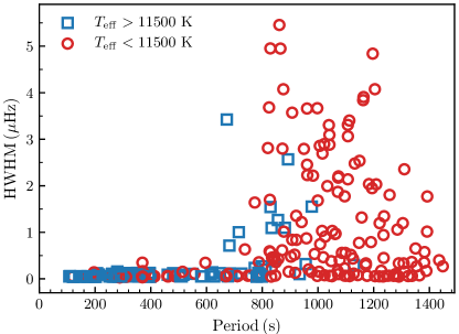
Figure 1: Observed Fourier width versus period for modes in DAVs observed with Kepler and K2. The blue squares and red circles denote modes in stars with $T_{\rm eff}>11$,500 K and $T_{\rm eff}<11$,500 K, respectively.

2 The Data

The extended length of observations ($\gtrsim$$75$ d for most stars) in the Kepler and K2 data sets results in a $1/T$ resolution in the power spectra of $<$$\,0.14\,\,\mu\rm Hz$; this sets the observable lower limit for the width of a peak in the Fourier transform. For the first time this enables the measurement of the widths of a large number of modes in many stars that are above this threshold (Bell et al., 2015). For their sample of 27 DAVs, Hermes et al. (2017) obtained follow-up spectroscopy with the WHT and SOAR telescopes; these spectra were fit using the techniques and models of Tremblay et al. (2011) to obtain values of $T_{\rm eff}$ and $\log\,g$ for each star.

Hermes et al. (2017) find that the Fourier width of modes, (HWHM, the half width at half maximum of a Lorentzian fit), is a strong function of the mode period, $P$. To summarize, they find that 1) modes with $\rm HWHM>0.3\,\mu$Hz have $P\gtrsim 800$ s and 2) modes with $P\lesssim 800$ s have $\rm HWHM<0.3\,\mu$Hz. This is illustrated in Figure 1, in which we have plotted mode width versus period for the linearly independent periods found in the sample of DAVs from Hermes et al. (2017). Modes from stars with $T_{\rm eff}>11$,500 K are shown as blue squares, while those from stars with $T_{\rm eff}<11$,500 K are shown as red circles. The fact that most of the modes with $\rm HWHM>0.3\,\mu$Hz are from the cooler population is not an independent piece of information since longer-period modes are typically found only in the cooler DAVs (Mukadam et al., 2006).

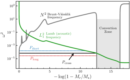
Figure 2: Schematic propagation diagram of a DAV white dwarf. A g-mode with a “short” period would have an outer turning point beneath the convection zone (blue dotted line), while one with a “long” period would have an outer turning point at the convection zone boundary (red dotted line). The crossover point between these two regimes is given by a mode with $P=P_{\rm cross}$ (black horizontal line).

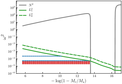
Figure 3: The outer propagation region for a model with the same parameters as EPIC 201806008. The dashed horizontal lines show the region of propagation that the observed modes would have in this model: the blue dashed lines denote modes observed to have $\rm HWHM<0.3\,\mu$Hz and the red dashed lines modes with $\rm HWHM>0.3\,\mu$Hz. The solid and dashed lines show the run of the Lamb (acoustic) frequency for $\ell=1$ and $\ell=2$ modes, respectively, to illustrate that higher-$\ell$ modes have lower values of $P_{\rm cross}$.

3 The Propagation Region

The region of propagation of $g$ modes (“gravity” or “buoyancy” modes) in a star is defined by the region in which $\omega^{2}<N^{2},L^{2}_{\ell}$, where $\omega=2\pi/P$ is the angular frequency of the mode, $N$ is the Brunt-Väisälä (buoyancy) frequency, $L_{\ell}$ is the Lamb (acoustic) frequency, and $\ell$ is the spherical degree of the mode. In Figure 2, we show a propagation diagram for a model, computed with MESA (Paxton et al., 2011, 2013, 2015, 2018, 2019). The black horizontal line denotes the region of propagation of a hypothetical mode whose period, $P_{\rm cross}$, is the minimum required for it to propagate to the base of the convection zone.

In Figure 3, we show the outer propagation region for a model with the same parameters as EPIC 201806008 ($\log\,g=8.02$, $T_{\rm eff}=10910\,$K). The dashed horizontal lines show the region of propagation that the observed modes would have in this model, where the blue dashed lines denote modes observed to have $\rm HWHM<0.3\,\mu$Hz and the red dashed lines modes with $\rm HWHM>0.3\,\mu$Hz. We note that, by using the convection model $\rm ML2/\alpha=0.42$, where $\alpha$ is the mixing length to pressure scale height ratio (see Böhm & Cassinelli, 1971), we can divide the modes into two groups: 1) narrow (blue) modes whose outer turning point is well beneath the convection zone, and 2) wide (red) modes that propagate all the way to the base of the convection zone. In other words, all the modes with $\rm HWHM>0.3\,\mu$Hz can be explained as propagating to the base of the convection zone, whereas all the modes with $\rm HWHM<0.3\,\mu$Hz have an outer turning point safely inside this point. Our hypothesis is that the long-period modes, through their interaction with the convection zone, will have systematically larger Fourier mode widths than the short-period modes. In the following sections we examine this statement more quantitatively.

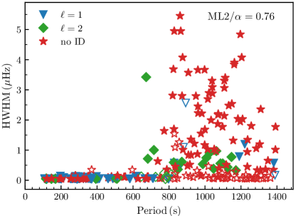
Figure 4: Similar to Figure 1, but with the following differences: blue triangles, green diamonds, and red stars denote modes that are identified as $\ell=1$, $\ell=2$, or unidentified modes, respectively. Using $P_{\rm cross}$ for each star as computed from its $T_{\rm eff}$ and $\log\,g$ values, modes with $P\geq P_{\rm cross}$ and $\rm HWHM>0.3\,\mu$Hz are shown as filled symbols, as are modes with $P<P_{\rm cross}$ and $\rm HWHM<0.3\,\mu$Hz. The opposite cases ($P<P_{\rm cross}$ and $\rm HWHM>0.3\,\mu$Hz, or $P\geq P_{\rm cross}$ and $\rm HWHM<0.3\,\mu$Hz) are shown as unfilled symbols.

4 A First Observational Test

Since the 27 DAVs in Hermes et al. (2017) have different atmospheric parameters, each star will have a different value of $P_{\rm cross}$ (note: $P_{\rm cross}$ is also a function of the $\ell$ value of each mode). Thus, for each mode in each star we calculate $P_{\rm cross}$ and from this we predict whether each observed mode in the star has a “wide, mottled” peak in the FT or a “narrow” peak. We assume the ML2 convection model of Böhm & Cassinelli (1971) with $\rm ML2/\alpha=0.76$. This value of $\alpha$ is taken from the 3D simulations of Tremblay et al. (2015) for a model with $T_{\rm eff}=11,500$ K and $\log\,g=8.0$.

We plot the results of this in Figure 4, where we have used different symbols for the different $\ell$ identifications: blue triangles for $\ell=1$ modes, green diamonds for $\ell=2$ modes, and red stars for unidentified modes. Unidentified modes are assumed to have $\ell=1$ for this analysis. Modes with wide peaks (i.e., $\rm HWHM>0.3\,\mu$Hz) are predicted to interact strongly with the convection zone. If this prediction is correct (i.e., if $P\geq P_{\rm cross}$ for the mode) then they are plotted with a filled symbol. If the prediction is incorrect, they are plotted with an unfilled symbol. Similarly, modes with narrow peaks (i.e., $\rm HWHM<0.3\,\mu$Hz) are predicted to interact weakly with the convection zone. If this prediction is correct (i.e., if $P<P_{\rm cross}$) then they are also plotted with a filled symbol; otherwise, an unfilled symbol is used. Thus, the filled symbols represent the modes whose widths are correctly predicted by our hypothesis. We find that this procedure correctly classifies the observed mode widths with an accuracy of $\sim\,$81%. While there is evidence that the value of $\alpha$ is a function of $T_{\rm eff}$ (Tremblay et al., 2015; Provencal et al., 2012), the percentage of correctly predicted modes is roughly constant for $\alpha$ in the range 0.6–0.9.

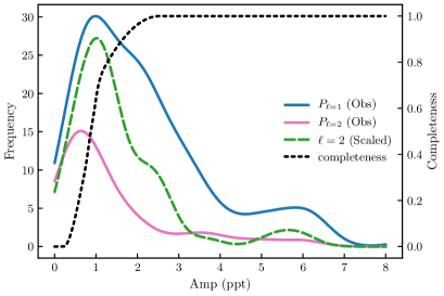
Figure 5: The observed distribution of modes identified as $\ell=1$ and 2 modes ($D_{\ell=1}$, $D_{\ell=2}$; blue and pink curves, respectively) as a function of amplitude. The $\ell=2$ (Scaled) curve (green dashed) shows the distribution that is obtained by scaling the $\ell=1$ distribution by the expected geometric amplitude ratio of $\ell=2$ and $\ell=1$ modes. We note that this results in a greater number of $\ell=2$ modes is observed. We note that the different detection thresholds of each star have been folded into a “completeness” curve, whose values are shown on the right vertical axis.

5 A Second Observational Test

Modes of different spherical degree ($\ell$) are also expected to interact with the convection zone differently as a function of period. Since the Lamb frequency of $\ell=2$ modes is larger than it is for $\ell=1$, for a fixed frequency $\ell=2$ modes have an outer turning point that is closer to the stellar surface, and are therefore more likely to strongly interact with the convection zone. If this can lead, in some cases, to not just a broadened peak in the FT but to a partial or complete suppression of the mode, then we would expect the number of $\ell=2$ modes to be suppressed by this mechanism.

Hermes et al. (2017) classify all of the statistically significant peaks in the FTs as either $\ell=1$, $\ell=2$, or undetermined. They were able to identify the $\ell$ value of 87 out of 201 independent modes in these DAVs (more than 40%), based on common frequency patterns in the Fourier transforms (e.g., the rotational splitting of multiplets and the period spacing of different radial overtones).

In Figure 5, we use “kernel density estimation” (kde) to estimate the density of modes as a function of the heights of the Lorentzians that were fit to them in the power spectrum, which we call their amplitude (Pedregosa et al., 2011). Only modes containing peaks with less than a 0.1% false alarm probability (FAP) and whose frequencies are not linear combinations of other mode frequencies are considered. As expected, the $\ell=1$ modes (blue curve) outnumber $\ell=2$ modes (pink curve). We next wish to test the hypothesis that there are as many $\ell=2$ as $\ell=1$ modes, but that the difference in observed numbers is solely due to geometric cancellation reducing their observed amplitudes below detection limits.

To test this, we divide the observed $\ell=1$ amplitudes by a factor of 2.4 to simulate the larger geometric cancellation of $\ell=2$ modes observed in the Kepler passband. The result is shown as the green dashed curve in Figure 5. We see that the number of $\ell=2$ modes obtained in this way exceeds those observed by a factor of more than 2. This could indicate that a mechanism in addition to pure geometric cancellation is limiting their number. Of course, without a way of identifying the unidentified modes that comprise $\sim\,60$% of this sample, it is not possible to conclusively demonstrate this.

Finally, we note that after scaling the observed $\ell=1$ amplitudes by the appropriate factors for $\ell=3$ and 4 ($\sim 26$ and 19, respectively), no modes are found to be above the $\rm FAP>0.1$% detection threshold. Thus, these data have nothing to say on the possible presence or amplitude distribution of these higher-$\ell$ modes.

6 Interaction with the Convection Zone

There are two main ways that a mode’s interaction with the outer convection zone could lead to a loss of its coherence. First, if a mode has a low enough frequency, its outer turning point will be the base of the convection zone. Since the base of the convection zone rises and falls with the surface temperature perturbations of the pulsations, the mode will sometimes have to travel a greater (or lesser) distance before being reflected, and in so doing it will acquire an extra phase $\Delta\phi$ (see Figure 6). A second effect that may play an even larger role is the Doppler shift of the wave caused by reflection from the base of the moving convection zone (see Figure 7). Essentially, the reflection causes a frequency shift of the reflected wave, which again leads to a phase mismatch when the wave next returns to the outer turning point.

In Montgomery et al. (2015), we showed that the extra phase acquired by a mode with quantum numbers $\{n,\ell\}$ due to a change in the size of its propagation cavity could be approximately calculated from the difference in period of this mode in two models ($\Delta P$) that differ only in the depth of their convection zones; this extra phase is given by

$$\Delta\phi_{\rm cav}=2\pi n\left(\frac{\Delta P}{P}\right).$$ (1)

We also calculate this phase difference by directly integrating the asymptotic expression for the radial wavenumber. From Gough (1993) we have that the asymptotic radial wavenumber $K(r)$ is given by

$$K^{2}(r)=\frac{\omega^{2}-\omega_{c}^{2}}{c^{2}}-\frac{L^{2}}{r^{2}}\left(1-\frac{N^{2}}{\omega^{2}}\right),$$ (2)

where $N$ is the Brunt-Väisälä frequency, $L^{2}\equiv\ell(\ell+1)$, $c$ is the sound speed, $\omega$ is the angular frequency of the mode, and $\omega_{c}$ is the acoustic cutoff frequency. The phase difference is then

$$\Delta\phi_{\rm cav} = 2\,\Delta\phi(r_{0},r_{\rm tp})$$ (3)

$$\equiv 2\left[\int_{r_{0}}^{r_{\rm tp}}K(r^{\prime})dr^{\prime}-\int_{r_{0}}^{r_{\rm tp0}}K_{0}(r^{\prime})dr^{\prime}\right],$$

where $r_{0}$ is a fiducial lower radius that remains fixed in mass and $r_{\rm tp}$ is the outer turning point of the mode; we note that $r_{\rm tp}$ is the actual radius at which reflection occurs (i.e., $K(r_{r_{\rm tp}})=0$). The second term in brackets on the RHS of equation 3 is the equilibrium value of the phase, and the first term is its instantaneous value. The factor of 2 is to account for the fact that the wave propagates from $r_{0}$ to $r_{\rm tp}$, and then back to $r_{0}$. For long period modes the reflection point is very near the base of the convection zone, but for shorter period modes $r_{\rm tp}$ is deeper in the model.

As previously mentioned, the Doppler shift caused by reflection from the base of the moving convection zone may lead to even larger phase shifts (see Figure 7). Essentially, the frequency shift due to reflection leads to a change in the wavelength of the wave (Montgomery et al., 2019). Thus, in traveling down to the inner turning point and back the mode no longer travels an exact integer number of wavelengths, arriving back at the outer turning point with a phase shift. Formally, the frequency perturbation is given by

$$\omega^{\prime}=\omega\,\left(1-v_{CZ}/v_{\rm gr}\right),$$ (4)

or, setting $\omega^{\prime}=\omega+\Delta\omega$,

$$\frac{\Delta\omega}{\omega}=-\frac{v_{CZ}}{v_{\rm gr}},$$ (5)

where $\omega$ is the frequency of the incident wave, $v_{CZ}$ is the velocity of the base of the convection zone, and $v_{\rm gr}$ is the group velocity of the wave at the base of the convection zone, given by $v_{\rm gr}\equiv\partial\omega/\partial K$.

Figure 6: Solid lines: the incoming wave incident on the base of the convection zone (vertical black lines); dashed lines: the waves reflected from the base of the convection zone. The blue curves represent the unperturbed case (reflection from leftmost vertical line) while the red curves show the effect of moving the base of the convection zone to the right (rightmost vertical line). The phase difference of the maxima of the reflected waves in these two cases is labeled as $\Delta\phi_{\rm cav}$, which is twice the phase shift $\Delta\phi$ labeled on the rightmost boundary.

Equation 5 is non-trivial to evaluate since $v_{\rm gr}$ formally goes to zero near the base of the convection zone. To remove this difficulty, we imagine the reflection occurring from a surface of constant phase well beneath the outer turning point, $r_{\rm tp}$, and we calculate the velocity of this surface, $v_{\rm surf}$. Using asymptotic formulae, we write this phase between the radii $r$ and $r_{\rm tp}$ as

$$\phi \equiv \int_{r}^{r_{\rm tp}}K(r^{\prime})dr^{\prime}$$ (6)

$$= \int_{r}^{r_{0}}K(r^{\prime})dr^{\prime}+\int_{r_{0}}^{r_{\rm tp}}K(r^{\prime})dr^{\prime},$$ (7)

where $r$ is the radius of the surface of constant phase, $K(r)$ is given by equation 2, and $r_{0}$ is a fiducial radius between $r$ and $r_{\rm tp}$ whose value is held constant.

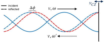
Figure 7: The change in the frequency of the reflected wave ($\omega\rightarrow\omega^{\prime}$) due to the velocity of the base of the convection zone ($v_{CZ}$). The blue curves represent the unperturbed case (reflection from a stationary boundary) while the red curve shows the effect of a convection zone base moving to the left. This frequency change leads to a change in the radial wavenumber of the wave, leading to a slow accumulation of phase difference as the wave propagates.

Setting $\partial\phi/\partial t=0$ in equation 7 and solving for $\partial r/\partial t$ yields

$$\frac{\partial r}{\partial t}=\frac{1}{K(r)}\frac{\partial}{\partial t}\int_{r_{0}}^{r_{\rm tp}}K(r^{\prime})dr^{\prime}.$$ (8)

Since $\partial r/\partial t$ represents the velocity of the surface of constant phase, we set $v_{\rm surf}=\partial r/\partial t$. Using this in place of $v_{CZ}$ in equation 5, we find

$$\frac{\Delta\omega}{\omega} = -\frac{v_{\rm surf}}{v_{\rm gr}}$$ (9)

$$= -\frac{1}{v_{\rm gr}K(r)}\frac{\partial}{\partial t}\int_{r_{0}}^{r_{\rm tp}}K(r^{\prime})dr^{\prime}.$$ (10)

Since we take the point $r$ to be safely beneath the outer turning point, we can use the asymptotic expression for the group velocity of g-modes, $v_{\rm gr}\approx-\omega/K(r)$. Substituting this in equation 10 yields

$$\Delta\omega=\frac{\partial}{\partial t}\int_{r_{0}}^{r_{\rm tp}}K(r^{\prime})dr^{\prime}.$$ (11)

We recognize the integral on the RHS of equation 11 as the mode phase between the point $r_{0}$ and the outer turning point. Since the time derivative only acts on the time-dependent variations of this quantity, we can rewrite it using $\Delta\phi(r_{0},r_{\rm tp})$ as defined in equation 3. Thus,

$$\Delta\omega = \frac{\partial}{\partial t}\left[\Delta\phi(r_{0},r_{\rm tp})\right]$$ (12)

$$\approx \langle\omega\rangle\,\Delta\phi(r_{0},r_{\rm tp}),$$

where we have replaced the time derivative with the factor $\langle\omega\rangle=2\pi/\langle P\rangle$, where $\langle P\rangle$ is a characteristic pulsation time scale for the ensemble of excited modes in the star (e.g., shorter for hotter stars, longer for cooler stars). Based on the results of Mukadam et al. (2006), we take $\langle P\rangle=300$ s for $T_{\rm eff}=12,000$ K, $\langle P\rangle=800$ s for $T_{\rm eff}=11,500$ K, and $\langle P\rangle=1000$ s for $T_{\rm eff}\leq 11,000$ K.

We note that the large time-dependent changes occur near the base of the convection zone, so $\Delta\phi(r_{0},r_{\rm tp})$ and therefore $\Delta\omega$ should be independent of the reference depth $r_{0}$. Numerically, we find that $\Delta\phi(r_{0},r_{\rm tp})$ changes by $<0.01$% as $r_{0}$ increases in depth by one mode wavelength. This is necessary since the calculated value of the frequency shift $\Delta\omega$ should be independent of the assumed distance from the base of the convection zone at which the calculation is made. For the calculations in Section 10, we arbitrarily choose this fiducial radius to be the point below the outer turning point at which $\phi=5\pi/4$; this is slightly over half a mode wavelength beneath the outer turning point.

The frequency difference given by equation 12, as the ray propagates down to the inner turning point and back out to the outer turning point, results in a total accumulated phase change of

$$\Delta\phi_{\rm dop} = 2\pi n\left(\frac{\Delta\omega}{\omega}\right)$$

$$= 2\pi n\,\frac{\langle\omega\rangle}{\omega}\,\,\Delta\phi(r_{0},r_{\rm tp})$$

These phase shifts lead to damping of the mode, as we show in the following section. Finally, using equation 3 we see that the phase change due to the doppler shift of the mode frequency can be related to that due to the changing size of the propagation cavity, i.e.,

$$\Delta\phi_{\rm dop}=n\pi\,\frac{\langle\omega\rangle}{\omega}\,\Delta\phi_{\rm cav}.$$ (13)

Since $n\geq 1$ and $\omega\approx\langle\omega\rangle$, we expect that the phase shift (and therefore the damping rate) due to the doppler shift to dominate that due to the changing cavity size.

We note here that this approach assumes that the traveling waves that comprise the mode propagate freely from the outer turning point down to the inner turning point and back again without encountering any regions of rapid spatial variation. Such regions could produce partial reflection and transmission of the waves, resulting in an unequal distribution of kinetic energy between the core and envelope regions. This “mode trapping” would lead to differential sensitivity of consecutive radial orders to phase shift effects. The fact that we ignore these possible internal reflections means that mode trapping effects will be suppressed in our damping calculations.

7 Theoretical Damping Rates

For the mode to be completely coherent, it needs to accumulate exactly $2\pi n$ radians of phase each time it propagates back and forth in the star. As shown in the previous section, a changing convection zone can upset this condition, leading to destructive interference and a change in amplitude given by

$$\frac{dA}{dt}=-\frac{A}{nP}\left(1-\cos\Delta\phi\right)$$ (14)

(see Montgomery et al., 2015). Assuming that $A\propto e^{-\gamma\,t}$, and averaging $\gamma$ over values of the phase shift from $-\Delta\phi$ to $+\Delta\phi$ gives

$$\gamma=\frac{1}{nP}\left(1-\frac{\sin\Delta\phi}{\Delta\phi}\right).$$ (15)

This is the equation we use to calculate the damping rates of modes given the amplitudes ($\Delta\phi$) of their phase shifts.

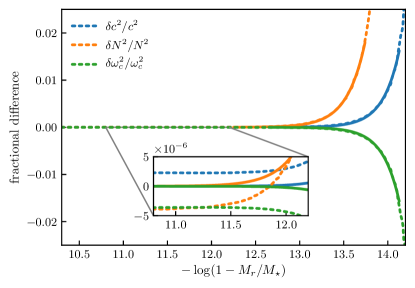
Figure 8: Difference of the pulsation quantities $N^{2}$, $c^{2}$, and $\omega_{c}^{2}$ in the region below the convection zones in neighboring models as a function of envelope mass; both models have $T_{\rm eff}$=12,000 K, and have ML2/$\alpha$ values of 0.859 and 0.885, respectively. The dotted lines show the difference in the relevant quantities while the solid lines show an exponential fit to this difference. As the inset shows, these differences do not decay to zero with depth.

8 Equilibrium Models

The WD models used in these calculations were computed with the MESA stellar evolution code (Paxton et al., 2011, 2013, 2015, 2018, 2019), and all the models assumed a mass of $0.6\,M_{\odot}$ (the mean mass of WDs in our sample is $0.62\,M_{\odot}$). Since the depth of the convection zone is the key parameter in this study, we have used the mixing length calibration of Tremblay et al. (2015) to set this parameter. Specifically, we have used the value of ML2/$\alpha_{\rm Schwa}$ from their Table 2 for the $\log\,g=8.0$ sequence interpolated to our $T_{\rm eff}$ values of interest.

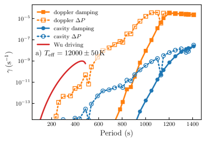
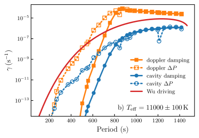
Figure 9: A comparison of the finite-amplitude damping rates for $\ell=1$ modes due to a changing cavity size (blue curves) and those due to Doppler shifting of the reflected wave (orange curves); the curves with filled symbols employ a direct integration of the wavenumber (equation 3) while those with open symbols use the period difference (equation 1) with $\Delta P$ calculated as described in section 9. We also show an estimate of the linear growth rates of these modes (red curves) based on scaled results in Wu (1998). Both sets of models have a mass of $0.6\,M_{\odot}$: those in a) have a $T_{\rm eff}$ of 12,000 K with an assumed pulsation amplitude of 50 K, while those in b) have a $T_{\rm eff}$ of 11,000 K with an assumed amplitude of $\pm$100 K.

To simulate the $T_{\rm eff}$ changes due to finite amplitude pulsations, we compute models with $T_{\rm eff}$ values centered on the equilibrium state, e.g., $T_{\rm eff}=12,000\pm 50\,$K. Since only the surface layers of the model correspond to these perturbed $T_{\rm eff}$ values, in a previous study (Montgomery et al., 2015) we spliced the outer portion of these models onto the equilibrium model. This was justified by the fact that the models rapidly converge with depth to nearly identical equilibrium structures so that the splicing produces no visible numerical artifacts. For the present study we adopt a different procedure. We first compute the depth of the convection zone with the perturbed $T_{\rm eff}$, say $T_{\rm eff}=12,050\,$K. We then find the value of ML2/$\alpha$ that reproduces this depth for the equilibrium $T_{\rm eff}$ of 12,000 K. We now identify this model as the “12,050 K” model since it has a convection zone depth that is identical to that of a “true” 12,050 K model. This approach has the advantage that no splicing of models is required.

9 Numerical Issues

For long-period modes whose outer turning points are very near the base of the convection zone, all of our approaches yield very similar results. That is, computing $\Delta\phi(r_{0},r_{\rm tp})$ from either the difference in oscillation periods of two neighboring models (equation 1) or using equation 3 to integrate the radial wavenumber in two models yields the same result. For instance, this can be seen in Figure 9b, in the agreement between the two sets of solid and dotted curves for periods greater than $\sim 1000$s.

For shorter-period modes that have an outer turning point farther beneath the convection zone, $\Delta\phi(r_{0},r_{\rm tp})$ depends on how quickly the differences in model quantities decay with depth. Denoting the differences between the two models (at constant mass coordinate) by $\delta$, $\delta N^{2}/N^{2}$, $\delta c^{2}/c^{2}$, and $\delta\omega_{c}^{2}/\omega_{c}^{2}$ initially decay exponentially with depth. However, instead of decaying to zero, they asymptote to a level of $\sim 10^{-6}$ (see inset in Figure 8). Since these models are designed to represent the same star at different times, the internal structure of the models (which should not be strongly affected by the changing surface convection zone) should be nearly identical. We force this to be true in our analysis by fitting the model differences with an exponential solution that decays to zero with increasing depth. We then add these differences back to the unperturbed model to create the new perturbed model, and these are the models used in integrating $\Delta\phi(r_{0},r_{\rm tp})$ in equation 3. This leads to a net decrease in the calculated damping rates of short-period modes, which were dominated by small, unphysical model differences in deeper layers.

In an asymptotic treatment, modes with outer turning points sufficiently far beneath the perturbed region will be completely unaffected by changes in the convection zone, and so will have zero calculated damping. However, in a full calculation the modes are global, and while they are evanescent in the region beneath the convection zone, they do still sample it. For long-period modes that propagate near the base of the convection zone, the period difference $\Delta P$ between models is dominated by the difference in convection zone depths, so we calculate $\Delta P$ as a direct difference of the pulsation periods of corresponding modes in the two models (Montgomery et al., 2015). For short-period modes, such period differences are dominated by numerical artifacts from the deeper layers, so we instead calculate the period difference via a variational approach (see equation 14.19 of Unno et al. 1989 and equation 5.80 of Christensen-Dalsgaard 2014), i.e.,

$$\Delta P=-\frac{\pi}{\omega^{3}}\,\frac{\int dM_{r}\,\delta N^{2}\,\xi_{r}^{2}}{\int dM_{r}\left[\,\xi_{r}^{2}+\ell(\ell+1)\,\xi_{h}^{2}\,\right]},$$ (16)

where $\xi_{r}$ and $\xi_{h}$ are the radial and horizontal displacements of the spatial eigenfunction, and $\delta N^{2}$ is the difference in the Brunt-Väisälä frequency between the two models. We then use equations 1, 12, 6, and 15 to calculate the phase shifts and damping associated with the period change of this mode.

10 Results for $\ell=1$

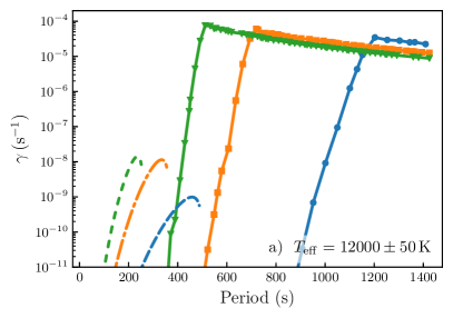
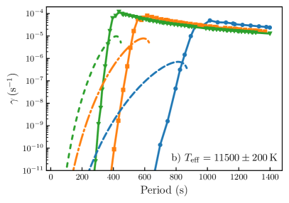
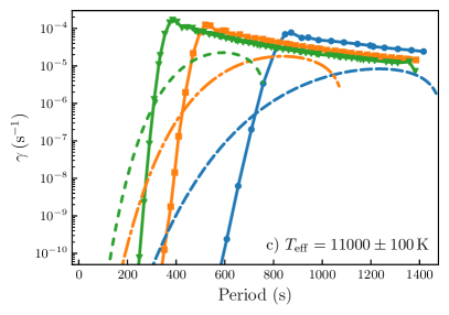
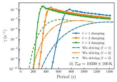
Figure 10: The same as Figure 9 showing the total damping results and estimated driving for a range of $\ell$ and $T_{\rm eff}$ values. Each plot contains results for $\ell=1$, 2, and 3 modes; panels (a)–(d) show results for $T_{\rm eff}$ values of 12,000 K, 11,500 K, 11,000 K, and 10,500 K, respectively. The $\pm$ values shown on each plot give the amplitude of the temperature perturbations assumed in calculating the nonlinear damping.

Combining equations 1, 3, 12, and 6 with equation 15, we compute finite-amplitude damping rates for $\ell=1$ pulsation modes. In Figures 9a,b we show the damping rates using $0.6\,M_{\odot}$ WD models at two different temperatures: $T_{\rm eff}=12$,000 K for Figure 9a, with assumed temperature excursions of $\pm 50$ K; and $T_{\rm eff}=11$,000 K for Figure 9b with assumed temperature excursions of $\pm 100$ K. After geometric cancellation, these cases correspond to observed luminosity perturbations of $\sim$1% and $\sim$2%, respectively. The blue curves with circular points show the damping rate due to the changing size of the g-mode cavity, while the orange curves with square points give the damping rate due to the Doppler shifting of the reflected wave’s frequency. In addition, curves with filled symbols employ a direct integration of the wavenumber (equation 3) while those with open symbols use the period difference (equation 1) with $\Delta P$ calculated as described in section 9. As can be seen, the two methods agree well for long-period modes, e.g., the blue filled and unfilled symbols in Figure 9b having $P>1000$s. The red curve in both plots is an estimate of the linear growth rates of these modes. These estimates are based on calculations by Wu (1998), as shown in Figures 5.5–5.8 of her thesis (see also Figure 6 of Wu & Goldreich 1999 and Figure 5 of Wu & Goldreich 2001).

The linear growth rates, by definition, do not depend on the amplitude of the pulsations, while the nonlinear damping mechanisms presented here do. As expected, we see that the damping due to the Doppler shift of the mode’s frequency is much larger than that due to the variation in the size of its g-mode cavity, for both models and sets of modes. In Figure 9a, this driving is larger than the assumed total damping for all periods that are driven, using either method of calculating the damping, while in Figure 9b, the driving exceeds the damping for periods less than $\sim\,$650s when the damping is calculated by direct integration of the radial wavenumber (filled points), with the driving exceeding the damping for periods less than $\sim\,$500s if the period difference method is used (unfilled symbols).

11 Damping as a Function of $\ell$ and $T_{\rm eff}$

We next examine these results both as a function of $\ell$ and $T_{\rm eff}$. In order to be conservative, in the remainder of this paper we use the damping estimates computed by direct integration of the radial wavenumber (e.g., filled symbols in Figures 9a,b), since these appear to provide a lower limit for these rates. In Figures 10a–d, we show the finite amplitude total damping rates as computed in the previous section for $\ell=1$, 2, and 3 modes. The different panels give the results for different values of $T_{\rm eff}$; for context, we also plot estimates of the driving rates based on Figures 5.5–5.8 from the thesis of Wu (1998). In Figure 10a, the range of $\ell=1$ modes assumed to be driven by convective driving is $P\sim$100–500 s (blue dashed curve), which is plausible for a $T_{\rm eff}=12000$ K model. For this case, we see that the damping is essentially insignificant for the driven modes. The same is true for $\ell=2$ and 3 modes.

Figure 10b is a slightly cooler case ($T_{\rm eff}\sim 11$,500 K), and the range of linearly driven $\ell=1$ modes is assumed to be $P\sim$100–900 s, with ranges of 100–600 s and 100–450 s for $\ell=2$ and 3, respectively. For the assumed 200 K amplitude, the damping mechanism could now potentially affect the amplitudes of the longest periods that are driven: 800 s for $\ell=1$, and 500 s and 350 s for $\ell=2$ and 3.

Finally, Figures 10c,d show the trends at cooler temperatures. As $T_{\rm eff}$ decreases, the driving decreases relative to the damping, implying smaller overall amplitudes. This has partially been accounted for by a decrease in the assumed amplitude of the pulsations, from $\pm 200$ K in Figure 10b to $\pm 100$ K in Figures 10c,d. For $\ell=1$, the period at which the driving equals the damping decreases from 800 s at $T_{\rm eff}=$11,500 K to 650 s and 550 s at $T_{\rm eff}=$11,000 K and 10,500 K, respectively. A similar trend can be seen for $\ell=2$ and 3 modes. Overall, these results imply that both the amplitudes seen in cooler models and their maximum periods should decrease. While the decrease in overall amplitude near the observed red edge has been previously noted (Mukadam et al., 2006), any observational decrease in maximum period with $T_{\rm eff}$ is less dramatic and has not been conclusively identified.

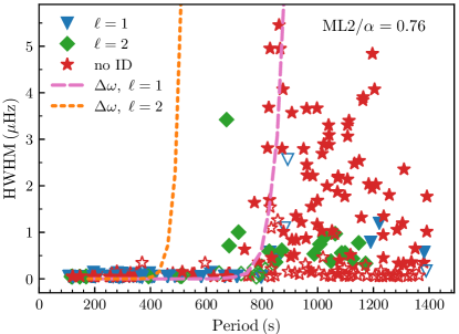
Figure 11: The same as Figure 4 but with a calculation of the expected mode widths for $\ell=1$ (dashed magenta curve) and $\ell=2$ (dotted orange curve) modes superimposed on the data. This calculation assumes a model with $T_{\rm eff}=11,500\,$K, $\log\,g=8.0$, $\alpha=0.76$, with the $T_{\rm eff}$ variations due to pulsation taken to be $\pm 200\,$K.

12 Mode Widths

Due to the nature of the stochastic excitation mechanism, the theoretical damping rates of solar-like pulsators provide a prediction for the observed Fourier widths of the modes. While this connection is less clear for pulsators with modes that are linearly unstable (such as the DAVs), we will attempt to calculate mode widths in the context of the damping mechanism presented above.

Equation 11 provides an estimate of the frequency change produced by a single interaction of a wave with the convection zone. If we interpret this frequency shift as an estimate of the width of the Fourier peak of the mode, we can calculate the expected widths for the pulsation modes in a given stellar model.

We show the results of such a calculation in Figure 11. The dashed magenta curve shows the frequency width for $\ell=1$ modes calculated in this way, while the dotted orange curve shows the width for $\ell=2$ modes. These calculations are based on the equilibrium model of Figure 10b ($T_{\rm eff}=11,500\,$K, $\log\,g=8.0$, $\rm ML2/\alpha=0.76$, with $T_{\rm eff}$ variations of $\pm 200\,$K). We see that there is a steep rise in the $\ell=1$ predicted widths at $\sim 800$ s, nominally coinciding with the observed rise seen in the data. We also note that the $\ell=2$ modes with $P\sim 700\,$s would not be expected to have large widths if they were $\ell=1$ modes, but are easily accounted for as $\ell=2$ modes. While certainly not the final word, this calculation provides a partial explanation for the observed rise in mode widths with increasing period.

13 Discussion

In the preceding sections we have shown that the modes with observed Fourier widths greater than 0.3 $\mu$Hz have longer periods ($P\gtrsim 800$ s), and that in most cases these modes are calculated to propagate all the way to the base of the surface convection zone in pulsating DA WDs. We have proposed mechanisms through which the convection zone can cause a lack of coherence in these modes. We find the dominant mechanism to be the Doppler shift of the mode frequency as it reflects off the time-dependent outer turning point. Preliminary results are that this mechanism is stronger near the observed red edge of the instability strip and may be important for the observed reduction in mode amplitudes there.

The phase shifts are a finite amplitude effect that naturally lead to damping. For hotter models ($T_{\rm eff}\gtrsim 12,000$ K), this damping is quite small and likely unimportant. On the other hand, for cooler models ($T_{\rm eff}<12,000$ K), this damping can be significant for longer period modes. The DAVs known to have stable pulsations coherent over a time period of years have short period pulsations ($P\lesssim 400\,$s) and are near the blue edge of the instability strip. From Figure 9a, we see that the proposed damping mechanism is quite small for these modes, which could be part of the reason these modes exhibit such extreme coherence. For cooler models, the damping is still small for the short-period modes, so the possibility remains that cooler pulsators could also harbor very stable pulsations in the form of low-period modes ($P<300$ s). These modes could have propagation regions sufficiently distant from the convection zone that they would still have extreme stability. Such modes, if they exist, could be used to asteroseismically trace secular evolution of cooler DAVs or expand the search for planets around white dwarfs with pulsation timing variations. As far as we are aware, no systematic search for such stable modes in cooler DAVs has been made, though some short-period modes do appear stable in cool DAVs over the span of months in Kepler/K2 observations.

We note that the calculations presented here could be improved in two respects. First, the convective driving rates based on the formalism of either Wu & Goldreich (1999) or Dupret et al. (2004) and Van Grootel et al. (2012) could be calculated for the stellar models employed here, leading to a consistent set of driving and nonlinear damping rates. In addition, the calculation of the difference in structure of neighboring models could be improved. Although the differences in their outer layers are dominated by their different convection zone depths, which our current calculations take into account, the differences deeper in the models will be directly due to the pulsation modes themselves. Thus, realistic eigenfunctions should be used to calculate the instantaneous structure of these models, which are then used in the subsequent analysis.

Finally, many DAVs observed with the Kepler and K2 missions undergo outbursts, increases in average brightness of 10–40% that can typically last from 5 to 15 hours (Bell et al., 2015; Hermes et al., 2015; Bell et al., 2017). While the best-known theory for this process involves a resonant transfer of energy from a driven parent mode to damped daughter modes as an amplitude threshold is reached (Luan & Goldreich, 2018; Wu & Goldreich, 2001), we speculate that the mechanism we have proposed involving phase shifts of reflected modes could be relevant as well. It is possible that some pulsators reach an amplitude threshold in which there is a slight increase in the damping, and this increased damping leads to a slight heating of the surface layers. This in turn causes a net thinning of the convection zone, leading to larger phase shift mis-matches, which leads to further damping, and the cycle reinforces itself. In addition, as the surface convection zone becomes thinner, radiative damping may play an important role in removing energy from the high overtone modes (Luan & Goldreich, 2018).

Nonlinear resonant energy transfer also appears to modify the frequency and amplitudes of modes on timescales shorter than expected from secular evolution, and this has been observed in a number of pulsating white dwarfs with long-baseline observations (e.g., Dalessio et al., 2013; Zong et al., 2016). However, the frequency changes of these effects are considerably smaller than those observed in the broadened mode line widths discussed here. Additionally, many of the DAVs with frequency changes incompatible with secular evolution occur in hotter stars with short-period ($<300\,$s) pulsations that should be relatively unaffected by the convection zone (e.g., Hermes et al. 2013).

14 Conclusions

We present a mechanism that may be relevant for the limitation of pulsation amplitudes in white dwarf stars for modes above a threshold period. As the convection zone changes depth during the pulsation cycle, the condition for coherent reflection of the outgoing traveling wave is slightly violated. In effect, this causes the amplitude of the mode (viewed as the superposition of inward- and outward-propagating components) to decrease, leading to damping. This mechanism should be present at some level in all pulsating WDs, and should be larger near the red edge of the DAV instability strip. In addition, this mechanism could possibly be relevant for other g-mode pulsators with surface convection zones (e.g., Gamma Doradus stars), or even large-amplitude pulsators such as high-amplitude delta Scuti stars (HADs) or RR Lyrae stars.

References

- Bell et al. (2015) Bell, K. J., Hermes, J. J., Bischoff-Kim, A., et al. 2015, ApJ, 809, 14, doi: 10.1088/0004-637X/809/1/14
- Bell et al. (2017) Bell, K. J., Hermes, J. J., Montgomery, M. H., et al. 2017, in Astronomical Society of the Pacific Conference Series, Vol. 509, 20th European White Dwarf Workshop, ed. P.-E. Tremblay, B. Gaensicke, & T. Marsh, 303
- Bischoff-Kim et al. (2008) Bischoff-Kim, A., Montgomery, M. H., & Winget, D. E. 2008, ApJ, 675, 1512, doi: 10.1086/526398
- Böhm & Cassinelli (1971) Böhm, K. H., & Cassinelli, J. 1971, A&A, 12, 21
-
Christensen-Dalsgaard (2014)
Christensen-Dalsgaard, J. 2014, Lecture Notes on Stellar Oscillations,
http://users--phys.au.dk/jcd/oscilnotes/Lecture_Notes_on_Stellar_Oscillations.pdf - Córsico et al. (2012) Córsico, A. H., Althaus, L. G., Miller Bertolami, M. M., et al. 2012, MNRAS, 424, 2792, doi: 10.1111/j.1365-2966.2012.21401.x
- Córsico et al. (2016) Córsico, A. H., Romero, A. D., Althaus, L. G., et al. 2016, J. Cosmology Astropart. Phys, 7, 036, doi: 10.1088/1475-7516/2016/07/036
- Dalessio et al. (2013) Dalessio, J., Sullivan, D. J., Provencal, J. L., et al. 2013, ApJ, 765, 5, doi: 10.1088/0004-637X/765/1/5
- Dupret et al. (2004) Dupret, M.-A., Grigahcène, A., Garrido, R., Gabriel, M., & Noels, A. 2004, in ESA Special Publication, Vol. 559, SOHO 14 Helio- and Asteroseismology: Towards a Golden Future, ed. D. Danesy, 207
- Gough (1993) Gough, D. O. 1993, in Astrophysical Fluid Dynamics - Les Houches 1987, ed. J.-P. Zahn & J. Zinn-Justin (Amsterdam: Elsevier Science Publishers), 399–560
- Hermes et al. (2013) Hermes, J. J., Montgomery, M. H., Mullally, F., Winget, D. E., & Bischoff-Kim, A. 2013, ApJ, 766, 42, doi: 10.1088/0004-637X/766/1/42
- Hermes et al. (2010) Hermes, J. J., Mullally, F., Winget, D. E., et al. 2010, AIP Conference Proceedings, 1273, 446, doi: 10.1063/1.3527860
- Hermes et al. (2015) Hermes, J. J., Montgomery, M. H., Bell, K. J., et al. 2015, ApJ, 810, L5, doi: 10.1088/2041-8205/810/1/L5
- Hermes et al. (2017) Hermes, J. J., Gänsicke, B. T., Kawaler, S. D., et al. 2017, ApJS, 232, 23, doi: 10.3847/1538-4365/aa8bb5
- Houdek & Dupret (2015) Houdek, G., & Dupret, M.-A. 2015, Living Reviews in Solar Physics, 12, 8, doi: 10.1007/lrsp-2015-8
- Hunter (2007) Hunter, J. D. 2007, Computing in Science & Engineering, 9, 90, doi: 10.1109/MCSE.2007.55
- Isern et al. (2008) Isern, J., García-Berro, E., Torres, S., & Catalán, S. 2008, ApJ, 682, L109, doi: 10.1086/591042
- Jones et al. (2001) Jones, E., Oliphant, T., Peterson, P., et al. 2001, SciPy: Open source scientific tools for Python. http://www.scipy.org/
- Kepler et al. (2005) Kepler, S. O., Costa, J. E. S., Castanheira, B. G., et al. 2005, ApJ, 634, 1311, doi: 10.1086/497002
- Kleinman et al. (1998) Kleinman, S. J., Nather, R. E., Winget, D. E., et al. 1998, ApJ, 495, 424, doi: 10.1086/305259
- Kumar & Goldreich (1989) Kumar, P., & Goldreich, P. 1989, ApJ, 342, 558, doi: 10.1086/167616
- Luan & Goldreich (2018) Luan, J., & Goldreich, P. 2018, ApJ, 863, 82, doi: 10.3847/1538-4357/aad0f4
- Montgomery et al. (2019) Montgomery, M. H., Hermes, J. J., & Winget, D. E. 2019, in 21st European Workshop on White Dwarfs, ed. B. G. Castanheira, Z. Vanderbosch, & M. H. Montgomery
- Montgomery et al. (2015) Montgomery, M. H., Romero, A. D., & Córsico, A. H. 2015, in Astronomical Society of the Pacific Conference Series, Vol. 493, 19th European Workshop on White Dwarfs, ed. P. Dufour, P. Bergeron, & G. Fontaine, 181
- Mukadam et al. (2006) Mukadam, A. S., Montgomery, M. H., Winget, D. E., Kepler, S. O., & Clemens, J. C. 2006, ApJ, 640, 956, doi: 10.1086/500289
- Mullally et al. (2003) Mullally, F., Mukadam, A., Winget, D. E., Nather, R. E., & Kepler, S. O. 2003, in NATO ASIB Proc. 105: White Dwarfs, 337
- Mullally et al. (2008) Mullally, F., Winget, D. E., Degennaro, S., et al. 2008, ApJ, 676, 573, doi: 10.1086/528672
- Oliphant (2006) Oliphant, T. E. 2006, A guide to NumPy, Vol. 1 (Trelgol Publishing USA)
- Paxton et al. (2011) Paxton, B., Bildsten, L., Dotter, A., et al. 2011, ApJS, 192, 3, doi: 10.1088/0067-0049/192/1/3
- Paxton et al. (2013) Paxton, B., Cantiello, M., Arras, P., et al. 2013, ApJS, 208, 4, doi: 10.1088/0067-0049/208/1/4
- Paxton et al. (2015) Paxton, B., Marchant, P., Schwab, J., et al. 2015, ApJS, 220, 15, doi: 10.1088/0067-0049/220/1/15
- Paxton et al. (2018) Paxton, B., Schwab, J., Bauer, E. B., et al. 2018, ApJS, 234, 34, doi: 10.3847/1538-4365/aaa5a8
- Paxton et al. (2019) Paxton, B., Smolec, R., Schwab, J., et al. 2019, ApJS, 243, 10, doi: 10.3847/1538-4365/ab2241
- Pedregosa et al. (2011) Pedregosa, F., Varoquaux, G., Gramfort, A., et al. 2011, Journal of Machine Learning Research, 12, 2825
- Provencal et al. (2012) Provencal, J. L., Montgomery, M. H., Kanaan, A., et al. 2012, ApJ, 751, 91, doi: 10.1088/0004-637X/751/2/91
- Tremblay et al. (2011) Tremblay, P.-E., Bergeron, P., & Gianninas, A. 2011, ApJ, 730, 128, doi: 10.1088/0004-637X/730/2/128
- Tremblay et al. (2015) Tremblay, P.-E., Ludwig, H.-G., Freytag, B., et al. 2015, ApJ, 799, 142, doi: 10.1088/0004-637X/799/2/142
- Unno et al. (1989) Unno, W., Osaki, Y., Ando, H., Saio, H., & Shibahashi, H. 1989, Nonradial oscillations of stars (Tokyo: University of Tokyo Press)
- Van Grootel et al. (2012) Van Grootel, V., Dupret, M.-A., Fontaine, G., et al. 2012, A&A, 539, A87, doi: 10.1051/0004-6361/201118371
- Winget et al. (2015) Winget, D. E., Hermes, J. J., Mullally, F., et al. 2015, in Astronomical Society of the Pacific Conference Series, Vol. 493, 19th European Workshop on White Dwarfs, ed. P. Dufour, P. Bergeron, & G. Fontaine, 285
- Wu (1998) Wu, Y. 1998, PhD thesis, California Institute of Technology
- Wu & Goldreich (1999) Wu, Y., & Goldreich, P. 1999, ApJ, 519, 783, doi: 10.1086/307412
- Wu & Goldreich (2001) —. 2001, ApJ, 546, 469, doi: 10.1086/318234
- Zong et al. (2016) Zong, W., Charpinet, S., Vauclair, G., Giammichele, N., & Van Grootel, V. 2016, A&A, 585, A22, doi: 10.1051/0004-6361/201526300