Single Image Depth Estimation Trained via Depth from Defocus Cues

Abstract

Estimating depth from a single RGB images is a fundamental task in computer vision, which is most directly solved using supervised deep learning. In the field of unsupervised learning of depth from a single RGB image, depth is not given explicitly. Existing work in the field receives either a stereo pair, a monocular video, or multiple views, and, using losses that are based on structure-from-motion, trains a depth estimation network. In this work, we rely, instead of different views, on depth from focus cues. Learning is based on a novel Point Spread Function convolutional layer, which applies location specific kernels that arise from the Circle-Of-Confusion in each image location. We evaluate our method on data derived from five common datasets for depth estimation and lightfield images, and present results that are on par with supervised methods on KITTI and Make3D datasets and outperform unsupervised learning approaches. Since the phenomenon of depth from defocus is not dataset specific, we hypothesize that learning based on it would overfit less to the specific content in each dataset. Our experiments show that this is indeed the case, and an estimator learned on one dataset using our method provides better results on other datasets, than the directly supervised methods.

1 Introduction

In classical computer vision, many depth cues were used in order to recover depth from a given set of images. These shape from X methods include structure-from-motion, which is based on multi-view geometry, shape from structured light, in which the known light source plays the role of an additional view, shape from shadow, and most relevant to our work, shape from defocus. In machine learning based computer vision, the interest has mostly shifted into depth from a single image, treating the problem as a multivariant image-to-depth regression problem, with an additional emphasis on using deep learning.

Learning depth from a single image consists of two forms. There are supervised methods, in which the target information (the depth) is explicitly given, and unsupervised methods, in which the depth information is given implicitly. The most common approach in unsupervised learning is to provide the learning algorithm with stereo pairs or other forms of multiple views [37, 41]. In these methods, the training set consists of multiple scenes, where for each scene, we are given a set of views. The output of the method, similar to the supervised case, is a function that given a single image, estimates depth at every point.

In this work, we rely, instead of multiple view geometry, on shape from defocus. The input to our method, during training, is an all-in-focus image and one or more focused images of the same scene from the same viewing point. The algorithm then learns a regression function, which, given an all-in-focus image, estimates depth by reconstructing the given focused images. In classical computer vision, research in this area led to a variety of applications [44, 35, 32], such as estimating depth from mobile phone images [33]. A deep learning based approach was presented by Anwar et al. [1] who employ synthetic focus images in supervised depth learning, and an aperture supervision depth learning by Srinivasan et al. [31], who employ lightfield images in the same way we use defocus images.

Our method relies on a novel Point Spread Function (PSF) layer, which preforms a local operation over an image, with a location dependent kernel which is computed “on-the-fly”, according to the estimated parameters of the PSF at each location. More specifically, the layer receives three inputs: an all-in-focus image, estimated depth-map and camera parameters, and outputs an image at one specific focus. This image is then compared to the training images to compute a loss. Both the forward and backward operations of the layer are efficiently computed using a dedicated CUDA kernel. This layer is then used as part of a novel architecture, combining the successful ASPP architecture [5, 9]. To improve the ASPP block, we add dense connections [16], followed by self-attention [42].

We evaluate our method on all relevant benchmarks we were able to obtain. These include the flower lightfield dataset and the multifocus indoor and outdoor scene dataset, for which we compare the ability to generate unseen focus images with other methods. We also evaluate on the KITTI, NYU, and Make3D, which are monocular depth estimation datasets. In all cases, we show an improved performance in comparison to methods with a similar level of supervision, and performance that is on par with the best directly supervised methods on KITTI and Make3D datasets. We note that our method uses focus cues for depth estimation, hence the task of defocusing for itself is not evaluated.

When learning depth from a single image, the most dominant cue is often the content of the image. For example, in street view images one can obtain a good estimate of the depth based on the type of object (sidewalk, road, building, car) and its location in the image. We hypothesize that when learning from focus data, the role of local image statistics becomes more dominant, and that these image statistics are more global between different visual domains. We therefore conduct experiments in which a depth estimator trained on one dataset is evaluated on another. Our experiments show a clear advantage to our method, in comparison to the state-of-the-art supervised monocular method of [9].

2 Related Work

Learning based monocular depth estimation

In monocular depth estimation, a single image is given as input, and the output is the predicted depth associated with that image. Supervised training methods learn from the ground truth depth directly and the so-called unsupervised methods employ other data cues, such as stereo image pairs. One of the first methods in the field was presented by Saxena et al. [27], applying supervised learning and proposed a patch-based model and Markov Random Field (MRF). Following this work, a variety of approaches had been presented using hand crafted representations [29, 18, 26, 11]. Recent methods use convolutional neural networks (CNN), starting from learning features for a conditional random field (CRF) model as in Liu et al. [22], to learning end-to-end CNN models refined by CRFs, as in [2, 40].

Many models employ an autoencoder structure [7, 12, 17, 19, 39, 9], with an added advantage to very deep networks that employ ResNets [15]. Eigen et al. [8, 7] showed that using multi-scaled depth predictions helps with the decrease in spatial resolution, which happened in the encoder model, and improves depth estimation. Other work uses different loss for regression, such as the reversed Huber [24] used by Laina et al. [19] to lower the smoothness effect of the $L_{2}$ norm, and the recent work by Fu et al. [9] who uses ordinal regression for each pixel with their spacing-increasing discretization (SID) strategy to discretize depth.

Unsupervised depth estimation Modern methods for unsupervised depth estimation have relied on the geometry of the scene, Garg et al. [12] for example, proposed using stereo pairs for learning, introducing the differentiable inverse warping. Godard et al. [14] added the Left-Right consistency constraint to the loss function, exploiting another geometrical cue. Zhou et al. [43] learned, in addition the ego-motion of the scene, and GeoNet [41] also used the optical flow of the scene. Wang et al. [37] recently showed that using direct visual odometry along with depth normalization substantially improves performance on prediction.

Depth from focus/defocus The difference between depth from focus and depth from defocus is that, in the first case, camera parameters can be changed during the depth estimation process. In the second case, this is not allowed. Unlike the motion based methods above, these methods obtain depth using the structure of the optical geometry of the lens and light ray, as described in Sec. 3.1. Work in this field mainly focuses on analytical techniques. Zhuo et al. [44] for example, estimated the amount of spatially varying defocus blur at edge locations. The use of Coded Aperture had been proposed by [20, 36, 30] to improve depth estimation. Later work in this field, such as Suwajanakorn et al. [33], Tang et al. [35] and Surh et al. [32] employed focal stacks — sets of images of the same scene with different focus distances — and estimated depth based on a variety of blurring models, such as the Ring Difference Filter [32]. These methods first reconstruct an all-in-focus image and then optimize a depth map that best explains the re-rendering of the focal stack images out of the all-in-focus image.

There are not many deep learning works in the field. Srinivasan et al. [31] presented a new lightfield dataset of flower images. They used the ground truth lightfield images to render focused images and employed a regression model to estimate depth from defocus by reconstruction of the rendered focused images.While Srinivasan et al. [31] did not compare to other RGB-D datasets [13, 27, 28, 23], their method can take as input any all-in-focus image. We evaluate [31] rendering process using our network on the KITTI dataset. Anwar et al. [1] utilized the provided depth of those datasets to integrate focus rendering within a fully supervised depth learning scheme.

3 Differentiable Optical Model

We review the relevant optical geometry on which our PSF layer relies and then move to the layer itself.

3.1 Depth From Defocus

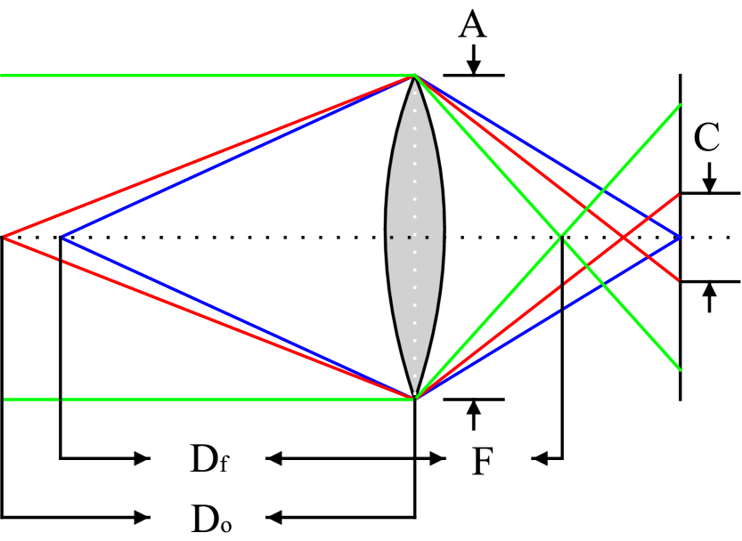
(a) Lens illustration

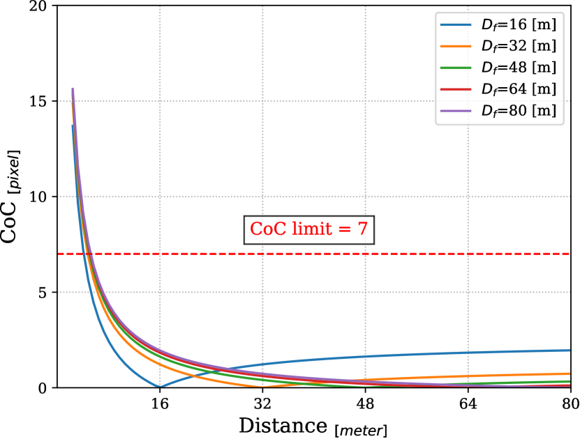
(b) CoC - KITTI

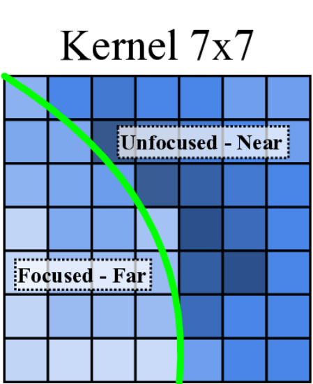
(c) CoC - KITTI

Figure 1: (a) Illustration of lens principles. Blue beams represent an object in focus. Red beams represent an object further away and out of focus. See text for symbol definitions. (b) CoC diameter w.r.t. object distance as seen in KITTI. Camera settings are: $N=2.8$, $F=35$, and $s=2$. (c) Sample blur kernel. Green line represents depth edge, Blue colors represent the relative blur contribution w.r.t. CoC.

Depth from focus methods are mostly based on the thin-lens model and geometry, as shown in Fig. 1(a). The figure illustrates light rays trajectories and the blurring effect made by out-of-focus objects. The plane of focus is defined such that light rays emerging from it towards the lens fall at the same point on the camera sensor plane. An object is said to be in focus, if its distance from the lens falls inside the camera’s depth-of-field (DoF), which is the distance about the plane of focus where objects appear acceptably sharp by the human eye. Objects outside the DoF appear blurred on the image plane, an effect caused by the spread of light rays coming from the unfocused objects and forming what is called the “Circle-Of-Confusion” (CoC), as marked by C in Fig. 1(a). In this paper, we will use the following terminology: an all-in-focus image is an image where all objects appear in focus, and a focused image is one where blurring effects caused by the lens configuration are observed.

In this model, we consider the following parameters to describe a specific camera: focal-length $F$, which is the distance between the lens plane and the point where initially parallel rays are brought to a focus, aperture $A$, which is the diameter of the lens (or an opening through which light travels), and the plane of focus $D_{f}$ (or focus distance), which is the distance between the lens plane and the plane where all points are in focus. Following the thin-lens model, we define the size of blur, i.e., the diameter of the CoC, which we denote as $C_{mm}$, according to the following equation:

$$C_{mm}=A\frac{|D_{o}-D_{f}|}{D_{o}}\frac{F}{D_{f}-F}$$ (1)

where $D_{o}$ is the distance between an object to the lens plane, and $A=F/N$ where $N$ is what is known as the f-number of the camera. While CoC is usually measured in millimeters ($C_{mm}$), we transform its size to pixels by considering a camera pixel-size of $p=5.6\mu m$ as in [3], and a camera output scale $s$, which is the ratio between sensor size and output image size. The final CoC size in pixels $C$ is computed as follows:

$$C=\frac{C_{mm}}{p\cdot s}.$$ (2)

The CoC is directly related to the depth, as illustrated in Fig. 1(b), where each line represents a different focus distance $D_{f}$. As can be seen, the relation is not one-to-one and will cause ambiguity in depth estimation. Moreover, different camera settings are required for different scenes in terms of the scene’s maximum depth, i.e. for KITTI, we consider maximum depth of 80 meters, and 10 meters for NYU. We also consider a constant f-number of $N=2.8$ and a different focal-length for all datasets, in order to lower depth ambiguity by lowering the DoF range (see Sec. 5.2 for more details).

We now refer to one more measurement named CoC-limit, defined as the largest blur spot that will still be perceived by the human eye as a point, when viewed on a final image from a standard viewing distance. The CoC-limit also limits the kernel size used for rendering and is, therefore, highly influential on the run time (bigger kernels lead to more computations). We employ a kernel of size $7\times 7$, which reflects a standard CoC-limit of $0.061mm$.

In this work, following [33, 35], we consider the blur model to be a disc-shaped point spread function (PSF), modeled by a Gaussian kernel with radius $r=C/2$ and kernel’s location indices $u,v$:

$$G(u,v,r)=\frac{1}{2\pi r^{2}}\exp\bigg{(}-\bigg{(}\frac{u^{2}+v^{2}}{2r^{2}}\bigg{)}\bigg{)}$$ (3)

Because we work in pixel space, if the diameter is less then one pixel ($C<1$), we ignore the blurring effect.

According to the above formulation, a focused image can be generated from an all-in-focus image and depth-map, as commonly done in graphics rendering. Let $I$ be an all-in-focus image and $J$ be a rendered focused image derived from depth-map $D_{o}$, CoC-map $C$, camera parameters $A$, $F$ and $D_{f}$, we define $J$ as follows:

$$\mathcal{F}_{x,y}(u,v) =\frac{2}{\pi C_{x,y}^{2}}\exp\bigg{(}-2\bigg{(}\frac{u^{2}+v^{2}}{C_{x,y}^{2}}\bigg{)}\bigg{)}$$ (4)

$$J_{x,y}: =(I\circledast F)$$ (5)

$$=\frac{\int\limits_{u,v\in\Omega}I_{x-u,y-v}\mathcal{F}_{x-u,y-v}(u,v)dudv}{\int\limits_{u^{\prime},v^{\prime}\in\Omega}\mathcal{F}_{x-u^{\prime},y-v^{\prime}}(u^{\prime},v^{\prime})du^{\prime}dv^{\prime}},$$

where $\Omega$ is an offsets set related to a kernel of size $m\times m$:

$$\Omega:=\left\{(u,v):\;u,v\in\bigg{[}-\frac{m}{2},\dots,0,\dots,\frac{m}{2}\bigg{]}\in\mathbb{N}\right\}$$ (6)

We denote by $\circledast$ the convolution operation with a functional kernel $\mathcal{F}$, by $(x,y)$ the image location indices, and by $(u,v)$ the offset indices bounded by the kernel size.

Based on Eq. 5, given a set of focused images of the same scene, one may optimize a model to predict the all-in-focus image and the depth map. Alternatively, given a focused image and its correspondent all-in-focus image, we predict the scene depth by reconstructing the focused image.

While [31] uses a weighted sum of disk kernels to render blur, our blur kernel is a Gaussian composition of different blur contributions from all neighbors (Eq. 5) where each kernel coefficient is calculated by a Gaussian function w.r.t. a different estimated CoC, as illustrated in Fig. 1(c).

3.2 The PSF Convolutional layer

The PSF layer we employ can be seen as a particular case of the locally connected layers of [34], with a few differences: first, in the PSF layer, the same operator is applied across all channels, while in the locally-connected layer, as well as in conventional layers (excluding depth-convolution [6]), the local operator varies between the input channels. Additionally, The PSF layer does not sum the outcomes, and returns the same number of channels in the output tensor as in the input tensor.

The PSF convolutional layer, designed for the task of Depth from Defocus (DfD), is based on Eq. 5, where kernels vary between locations and are calculated “on-the-fly”, according to function $\mathcal{F}$, which is defined in Eq. 4. The kernel is, therefore, a local function of the object’s distance, with a blur kernel applied to out-of-focus pixels. The layer takes as input an all-in-focus image $I$, depth-map $D_{o}$ and the camera parameters vector $\rho$, which contains the aperture $A$, the focal length $F$ and the focal depth $D_{f}$. The layer then outputs a focused image $J$. As mentioned before, we fix the near and far distance limits to fit each dataset and use the fixed pixel size mentioned above. The rendering process begins by first calculating the CoC-map $C$ according to Eq. 1, and then applying the functional kernel convolution defined in Eq. 5. We implement the following operation in CUDA and compute its derivative as follows:

$$\bigg{(}\frac{\partial J_{s,t}}{\partial I_{x,y}}\bigg{)} =\frac{\mathcal{F}_{x,y}(u,v)}{\int\limits_{u^{\prime},v^{\prime}\in\Omega}\mathcal{F}_{s-u^{\prime},t-v^{\prime}}(u^{\prime},v^{\prime})du^{\prime}dv^{\prime}}$$ (7)

$$\bigg{(}\frac{\partial J_{s,t}}{\partial C_{x,y}}\bigg{)} =\frac{\xi_{x,y}(u,v)(I_{x,y}-J_{s,t})\mathcal{F}_{x,y}(u,v)}{\int_{u^{\prime},v^{\prime}\in\Omega}\mathcal{F}_{s-u^{\prime},t-v^{\prime}}(u^{\prime},v^{\prime})du^{\prime}dv^{\prime}}$$ (8)

$$\xi_{x,y}(u,v): =\frac{4(u^{2}+v^{2})-2C_{x,y}^{2}}{C_{x,y}^{3}}$$ (9)

A detailed explanation of the forward and backward pass is provided in the supplementary material.

4 Approach

In this section, we describe the training method and the model architecture, which extends the ASPP architecture to include both self-attention and dense connections. We then describe the training procedure.

4.1 General Architecture and the Training Loss

Let $J$ be a (real-world) focused version of $I$, and $\bar{J}$ be a predicted focused version of $I$. We train a regression model to minimize the reconstruction loss of $J$ and $\bar{J}$.

We define two networks, $f$ and $g$, for depth estimation and focus rendering respectively. While $f$ is learned, $g$ implements Eq. 4 and 5. Both networks take part in the loss, and backpropagation through $g$ is performed using Eq. 7, 8.

The learned network $f$ is applied to an all-in-focus image $I$ and returns a predicted depth $\bar{D}_{o}=f(I)$. The fixed network $g$ consists of the PSF layer, as described in Sec. 3.2. It takes as input an all-in-focus $I$, a depth (estimated or not) $D_{o}$ and the camera parameters vector $\rho$. It outputs $J=g(I,D_{o},\rho)$, which is a focused version of $I$ according to depth $D_{o}$ and camera parameters $\rho$. We distinguish between a rendered focus image from ground truth depth $D_{o}$ which we denote as $J$ (also used for real focused imaged), and rendered focused image from predicted depth $\bar{D}_{o}$, which we denote as $\bar{J}=g(I,\bar{D}_{o},\rho)$.

The training procedure has two cases, training with real data or on generated data, depending on the training dataset at hand. In both cases, training is performed end-to-end by running $f$ and $g$ sequentially. First, $f$ is applied to an all-in-focus image $I$ and outputs the predicted depth-map $\bar{D}_{o}$. Using this map, the all-in-focus image and camera parameters $\rho$, $g$ renders the predicted focused image $\bar{J}$. A reconstruction error is then applied with $J$ and $\bar{J}$, where for the case of depth-based datasets, we render the training focused images $J$, according to ground truth depth-map $D_{o}$ and camera specifications $\rho$. Fig. 2 shows the training scheme, where the blue dashed rectangle illustrates the second case, where $J$ is rendered from the ground truth depth.

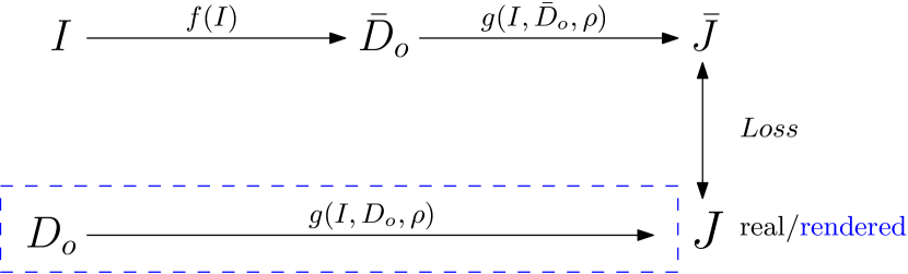
Figure 2: Training scheme. Blue region represents the rendering branch, which is used for depth-based datasets.

In the first case, since we compare with the work of [31], we use a single focused image during training, although more can be used. In the second case, we compare with fully supervised methods, that benefit from a direct access to the depth information, and we report results for 1, 2, 6 and 10 rendered focused images.

Training loss We first consider the reconstruction loss and the depth smoothness [38, 14] w.r.t. the input image $I$, the predicted focused image $\bar{J}$, the focused image $J$, and the estimated depth map $\bar{D}_{o}$:

$$\mathcal{L}_{rec}=\frac{1}{N}\sum{}{}\alpha\frac{1-SSIM(\bar{J},J)}{2}+(1-\alpha)\|\bar{J}-J\|_{1}$$ (10)

$$\mathcal{L}_{smooth}=\frac{1}{N}\sum{}{}|\partial_{x}\bar{D}_{o}|e^{-|\partial_{x}I|}+|\partial_{y}\bar{D}_{o}|e^{-|\partial_{y}I|}$$ (11)

where $SSIM$ is the Structural Similarity measure [38], and $\alpha$ controls the balance w.r.t. to $L_{1}$ loss.

The reconstruction loss above does not take into account the blurriness in some parts of image $J$, which arise from regions that are out of focus. We, therefore, add a sharpness measure $S(I)$ similar to [25], which considers the sharpness of each pixel. It contains three parts: (i) the image Laplacian $\Delta I:=\partial_{x}^{2}I+\partial_{y}^{2}I$, (ii) the image Contrast Visibility $C(I):=\bigg{|}\frac{I-\mu_{I}}{\mu_{I}}\bigg{|}$, and (iii) the image Variance $V(I):=(I-\mu_{I})^{2}$, where $\mu_{I}$ is the average pixel value in a window of size $7\times 7$ pixels. The sharpness measure is given by $S(I)=-\Delta I-C(I)-V(I)$, and the loss term is:

$$\mathcal{L}_{sharp} =\|S(\hat{J})-S(J)\|_{1}.$$ (12)

The final loss term is then:

$$Loss=\lambda_{1}\mathcal{L}_{rec}+\lambda_{2}\mathcal{L}_{smooth}+\lambda_{3}\mathcal{L}_{sharp}$$ (13)

For all experiments, we set $\lambda_{1}=1,\lambda_{2}=10^{-3},\lambda_{3}=10^{-1}$.

4.2 Model Architecture

Figure 3: Dense ASPP with an added attention block.

Our network $f$ is illustrated in Fig. 3. It consists of an encoder-decoder architecture, where we rely on the DeepLabV3+ [4, 5] model, which was found to be effective for semantic segmentation and depth estimation tasks [9]. The encoder has two parts: a ResNet [15] backbone and a subsequent Atrous Spatial Pyramid Pooling (ASPP) module. Unlike [9], we do not employ a pretrained ResNet and learn it end-to-end.

The Atrous convolutions (also called dilated convolutions) add padding between kernel cells to enlarge the receptive field from earlier layers, while keeping the weight size constant. ASPP contains several parallel Atrous convolutions with different dilations. As advised in [5], we also replace all pooling layers of the encoder with convolution layers with an appropriate stride.

The loss is computed in the highest resolution, to support higher quality outputs. However, to comply with GPU memory constraints, the network takes as an input, a downsampled image of half the original size. The network’s output is then upsampled to the original image size.

Dense ASPP with Self-Attention The original ASPP consists of three or more independent layers - average pooling followed by $1\times 1$ convolution, $1\times 1$ convolution, and four Atrous layers. Each convolution layer has 256 channels and the four outputs of these layers, along with the pool+conv layer are concatenated together to form a tensor with channel size $C=1280$. We propose two additional modifications from different parts of the literature: dense connections [16] and self attention [42].

We add dense connections between the $1\times 1$ convolution and all Atrous convolution layers of the ASPP module, sequentially connecting all layers from smallest to the largest dilation layer. Each layer, therefore, receives as the input tensor not just the output of the previous layer, but the concatenation of the output tensors of all preceding layers. This is illustrated as the skip connection arrows in Fig. 3.

Self-Attention aims to integrate local features with their global dependencies, and as shown in previous work [42, 10], it improve results in image segmentation and generation. Our implementation is based on [10] dual-attention.

The decoder part of $f$ consists of three upsampling blocks, each having three convolution layers followed by bilinear upsampling. A skip connection from a low level layer of the backbone is concatenated with the input of the second block. The output of decoder is the predicted depth.

5 Experiments

We divide our experiments into two types, DoF supervision and DoF supervision from rendered data, as mentioned in the previous section. We further experiment with cross domain evaluation, where we evaluate our method in comparison to the state-of-the-art supervised method [9]. Here the models are trained on domain A and tested on domain B, denoted as $A\rightarrow B$. We show that learning depth from focus cues, though not achieving better results than the supervised methods - but comparable with top methods in KITTI and Make3D datasets, achieves better generalization expressed by higher results in cross domain evaluation.

The network is trained on a single Titan-X Pascal GPUs with batch size of 3, using Adam for optimization with a learning rate of $2\cdot 10^{-5}$ and weight decay of $4\cdot 10^{-5}$. The dedicated CUDA implementation of the PSF layer runs x80 faster than the optimized pytorch implementation.

The following five benchmarks are used:

Lightfield dataset [31] The dataset contains lightfield flowers and plants images, taken with a Lytro Illum camera. From the lightfield images, we follow the procedure of [31] to generate the all-in-focus and shallow DoF images, and split the dataset into 3143 and 300 images for train and test.

DSLR dataset [3] This dataset contains 110 images and ground truth depth from indoor scenes, with 81 images for training and 29 images for testing, and 34 images from outdoor scenes without ground truth depth. Each scene is acquired with two camera apertures: $N=2.8$ and $N=8$, providing focused and all-in-focus images.

KITTI [13] This benchmark contains RGB-D images taken in an outdoor environment at resolution of roughly $370\times 1226$ which we refer to as the full resolution output size. The train/test splits we employ follow Eigen et al. [8], with 23,000 training images and 697 test images. The input depth-maps and images are cropped, according to [8] to obtain valid depth values, and resized to half-size.

NYU DepthV2 [23] This benchmark contains about 120K indoor RGB and depth images captured with a Microsoft Kinect. The datasets consists of 249 scenes for training and 215 scenes for testing. We report results on 654 test images from a small subset of 1449 aligned RGB-depth pairs, as done in previous work.

Make3D [27, 28] The Make3D benchmark contains 534 RGB-depth pairs, split into 400 pairs for training and 134 for testing. The input images are provided at a high resolution, while the depth-maps are at low resolution. Therefore, data is resized to $460\times 345$, as proposed by [27, 28]. Following [27], results are evaluated in two settings: $C1$ for depth cap of 0-70, and $C2$ for depth cap 0-80.

5.1 Results

DoF supervision We first report results on the Lightfield dataset dataset, which provides focused and all-in-focus image pairs with no ground truth depth. The performance is evaluated using the PSNR and SSIM measures. Our results are shown in Tab. 1. As can be seen, we significantly outperform the literature baselines provided by  [31].

Algorithm	Supervision	PSNR	SSIM
Image Regression [31]	DoF	24.60	0.895
Multi-View [31]	DoF	34.49	0.960
Lightfield [31]	DoF	36.68	0.967
Compositional [31]	DoF	36.90	0.966
Ours	DoF	38.33	0.979

Table 1: Quantitative results on the Lightfield test set, reported as a mean value of PSNR and SSIM of the reconstructed focused image.

Rendered DoF supervision

Reference Image	Ground Truth	Wang [37]	F2	F6	F10

Figure 4: KITTI: Qualitative results on the KITTI Eigen Split. All images are cropped to the valid depth region as proposed in [8]. From left to right, reference image and ground truth, Wang et al. [37] and ours.

Algorithm	Supervision	Abs Rel	Sq Rel	RMSE	RMSE log	$\delta<1.25$	$\delta<1.25^{2}$	$\delta<1.25^{3}$
Godard et al. [14]	S	0.148	1.344	5.927	0.247	0.803	0.922	0.964
Geonet-ResNet [41]	M	0.155	1.296	5.857	0.233	0.793	0.931	0.973
Wang et al. [37]	M	0.151	1.257	5.583	0.228	0.810	0.936	0.974
Godard et al. [14]	S(K+CS)	0.114	0.898	4.935	0.206	0.861	0.949	0.976
Ours F1	DoF	0.141	1.473	5.187	0.221	0.846	0.953	0.981
Ours F2	DoF	0.129	0.722	4.233	0.183	0.856	0.960	0.985
Ours F6	DoF	0.114	0.671	4.144	0.172	0.867	0.963	0.987
Ours F10	DoF	0.110	0.666	4.186	0.168	0.880	0.966	0.988
Liu et al. [22]	Depth	0.202	1.614	6.523	0.275	0.678	0.895	0.965
Kuznietsov et al. [17]	Depth	0.113	0.741	4.621	0.189	0.862	0.960	0.986
DORN et al. [9]	Depth	0.072	0.307	2.727	0.120	0.932	0.984	0.994

Table 2: KITTI: Quantitative results on the KITTI Eigen split. Top - Unsupervised methods where ‘S’ and ‘M’ stands for stereo and video (monocular) supervision, and ‘K+CS’ stands for training with the added data from the CityScapes dataset. Middle - Our method. Bottom - Supervised methods.

Algorithm	Supervision	$C1$			$C2$
		Abs Rel	RMSE log10	RMSE	Abs Rel	RMSE log10	RMSE
Godard et al. [14]	S	0.443	0.156	11.513	-	-	-
Zhou et al. [43]	MS	0.383	0.478	10.470	-	-	-
Wang et al. [37]	MS	0.387	0.204	8.090	-	-	-
Ours F1	DoF	0.568	0.192	8.822	0.575	0.195	10.147
Ours F2	DoF	0.287	0.116	7.710	0.294	0.121	9.387
Ours F6	DoF	0.262	0.109	7.474	0.269	0.115	9.248
Ours F10	DoF	0.246	0.110	7.671	0.254	0.116	9.494
Li et al. [21]	Depth	0.278	0.092	7.120	0.279	0.102	10.27
MS-CRF [40]	Depth	0.184	0.065	4.380	0.198	-	8.56
DORN [9]	Depth	0.157	0.062	3.970	0.162	0.067	7.32

Table 3: Make3D: Quantitative results on Make3D [27, 28] dataset. Top - Unsupervised methods where ‘S’ and ‘M’ stands for stereo and video (monocular) supervision. Middle - Our method. Bottom - Supervised methods.

Algorithm	Supervision	Abs Rel	RMSE log10	RMSE	$\delta<1.25$	$\delta<1.25^{2}$	$\delta<1.25^{3}$
Ours F1	DoF	0.254	0.092	0.766	0.691	0.880	0.944
Ours F2	DoF	0.162	0.068	0.574	0.774	0.941	0.984
Ours F6	DoF	0.149	0.063	0.546	0.797	0.951	0.987
Ours F10	DoF	0.162	0.068	0.575	0.772	0.942	0.984
Li et al. [21]	Depth	0.143	0.063	0.635	0.788	0.958	0.991
MS-CRF [40]	Depth	0.121	0.052	0.586	0.811	0.954	0.987
DORN [9]	Depth	0.115	0.051	0.509	0.828	0.965	0.992

Table 4: NYU: Quantitative results on NYU V2 [23] dataset. Top - Our method. Bottom - Supervised methods.

For rendered DoF supervision, we consider four datasets [8, 27, 23, 3] with ground truth depth, where we render focused images with different focus distances. We denote by F1, F2, F6, F10 the four training setups, which differ by the number of rendered focused images used in training. The order in which focal distances are selected, is defined by the following focal sequence $[0.2,0.8,0.1,0.9,0.3,0.7,0.4,0.6,0.5,0.35]$, where each number represents the percent of the maximum depth used for each dataset. For example, F2 employs focal distances of 0.2 and 0.8 times the maximal depth.

We perform two types of evaluations. First, we evaluate our method for each dataset with different numbers of focused images during training, and compare our results with other unsupervised methods, as well as with supervised ones. The evaluation measures are those commonly used in the literature [13, 27, 28] and include various RMSE measures and a thresholded error rate.

Tab. 4 and 4 show that our method outperforms monocular and stereo supervision methods on the KITTI and Make3D dataset. This also holds when the previous methods are trained with additional data obtained from the Cityscapes dataset. In comparison to the depth supervised methods, we outperform all methods on KITTI, with the exception of [9], and outperform [9, 21] on Make3D. In Fig. 4, we present qualitative results of our method compared to the state-of-the-art unsupervised method [37] on the KITTI dataset. As can be seen in Tab. 4, there are no literature unsupervised methods reported for the NYU dataset, where we are slightly outperformed by the supervised methods.

We next preform cross domain evaluation compared to the published models of the state-of-the-art supervised method [9], where training is performed on KITTI or NYU, and tested on different datasets. These tests are meant to evaluate the specificity of the learned network to a particular dataset. Since the absolute depth differs between datasets, we evaluate the methods by computing the Pearson correlation metric. Results are shown in Tab. 5. As can be seen, when transferring from both KITTI and NYU, we outperform the directly supervised method. The gap is especially visible for the NYU network.

Transition	Algorithm	Correlation
KITTI $\rightarrow$ NYU	DORN [9]	0.423 $\pm$ 0.010
	Ours F1	0.121 $\pm$ 0.006
	Ours F10	0.429 $\pm$ 0.009
KITTI $\rightarrow$ Make3D	DORN [9]	0.616 $\pm$ 0.011
	Ours F1	0.484 $\pm$ 0.019
	Ours F10	0.642 $\pm$ 0.014
KITTI $\rightarrow$ D3Net	DORN [9]	0.145 $\pm$ 0.048
	Ours F1	0.148 $\pm$ 0.032
	Ours F10	0.275 $\pm$ 0.054
NYU $\rightarrow$ KITTI	DORN [9]	0.456 $\pm$ 0.006
	Ours F1	0.567 $\pm$ 0.006
	Ours F10	0.634 $\pm$ 0.005
NYU $\rightarrow$ Make3D	DORN [9]	0.250 $\pm$ 0.019
	Ours F1	0.249 $\pm$ 0.032
	Ours F10	0.456 $\pm$ 0.022
NYU $\rightarrow$ D3Net	DORN [9]	0.260 $\pm$ 0.054
	Ours F1	0.530 $\pm$ 0.048
	Ours F10	0.434 $\pm$ 0.052

Table 5: Quantitative results for cross domain evaluation. Models are trained on domain A and tested on domain B. Reported numbers are mean $\pm$ standard error.

We also provide cross-domain results for the outdoor images of the DSLR dataset, where no ground truth depth is provided, using the PSNR and SSIM metrics. Tab. 5 shows in this case that our method transfers better from NYU and only slightly better from KITTI in comparison to [9].

Transition	Algorithm	PSNR	SSIM
KITTI $\rightarrow$ DSLR	DORN [9]	24.95	0.823
	Ours F1	24.91	0.822
	Ours F10	24.98	0.826
NYU $\rightarrow$ DSLR	DORN [9]	24.73	0.749
	Ours F1	24.97	0.774
	Ours F10	24.97	0.773

Table 6: Quantitative results on the outdoor DSLR [3] test set, reported as mean value of PSNR and SSIM of the reconstructed focused image.

Model	F1	F2	F6	F10
ASPP	5.412	4.422	4.311	4.194
ASPP + D	5.285	4.351	4.170	4.190
ASPP + SA	5.387	4.402	4.232	4.188
Our	5.187	4.233	4.144	4.186

Table 7: A comparison on KITTI between the original ASPP and our dense ASPP with self-attention. We denote ‘D’ for Dense connections and ‘SA’ for Self-Attention. RMSE is shown for focused image stacks of different sizes.

Rendering	F1			F2
	Abs Rel	RMSE	$\delta<1.25$	Abs Rel	RMSE	$\delta<1.25$
[31]	0.489	12.395	0.293	0.636	11.177	0.230
[31]+BF	0.379	11.921	0.354	0.339	11.612	0.418
Ours	0.141	5.187	0.846	0.129	4.233	0.856

Table 8: A comparison on KITTI dataset between different blur methods on top of our network. BF= bilateral filtering.

(a)	(b)

Figure 5: (a) $\delta<1.25$, higher is better, for training F1 with different focus distance. (b) RMSE, lower is better.

5.2 Ablation Studies

The Effect of Focal Distance  Because the focus distance $D_{f}$ and DoF range are positively correlated, training with a far focus distance increases the DoF and puts a large range of distances in focus. As a result, focus cues are lowered, causing performance to decrease. In Fig. 5 we present, for the Make3D dataset, the accuracy of F1 training with different focus distances, where a clear decrease in performance is seen at mid-range $D_{f}$ and an increase afterward, as a result of the dataset maximum depth, capping the far DoF distance, i.e. lowering the DoF range, and increasing focus cues for closer objects.

Dense ASPP with Self-Attention We evaluate our dense ASPP with self-attention in comparison to three versions of the original ASPP model: vanilla ASPP, ASPP with dense connections and ASPP with self-attention. In order to differentiate between different ambiguity scenarios, training is preformed with the F1, F2, F6 and F10 methods. As can be seen in Tab 5, our model outperform the different ASPP versions. However, as the number of focused images increases, the gaps are reduced.

Different rendering methods To further compare with [31], we have conducted a test on the KITTI dataset, where we replaced our rendering network $g$ with their compositional rendering, and modified our depth network $f$’s last layer to output 80 depth probabilities (similar to [31]). From Tab. 5, the compositional method of [31] preforms poorly on KITTI in the F1 and F2 setting.

6 Conclusion

We propose a method for learning to estimate depth from a single image, based on focus cues. Our method outperforms the similarly supervised method [31] and all other unsupervised literature methods. In most cases, it matches the performance of directly supervised methods, when evaluated on test images from the training domain. Since focus cues are more generic than content cues, our method outperforms the state-of-the-art supervised method in cross domain evaluation on all available literature datasets.

We introduce a differentiable PSF convolutional layer, which propagates image based losses back to the estimated depth. We also contribute a new architecture that introduces dense connection and Self-Attention to the ASPP module. Our code is available as part of the supplementary material, and on GitHub https://github.com/shirgur/UnsupervisedDepthFromFocus.

Supplementary: Differentiable Gaussian PSF Layer

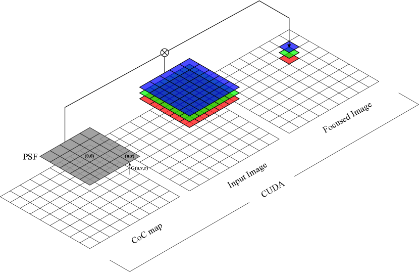
Figure 6: Illustration of the PSF convolution layer for focus rendering. each kernel is spatially computed from the CoC map and multiplied with the corespondent image patch both channel and element wise.

In this appendix we show the mathematical development of our PSF layer for backward and forward pass. For easy notation we define:

$$M_{x-i,y-j}:=M_{[}x-i,y-j]$$

where $M$ is any matrix or function, $(x,y)$ are location indices and $(u,v)$ are offsets. An illustration of the the PSF convolution is shown in Fig. 6.

Forward Pass: For a PSF kernel of size $m\times m$ where $m$ is odd, we consider an offsets set $\Omega$ of the form:

$$\Omega:=\left\{(u,v):\;u,v\in[-\frac{m}{2},\dots,0,\dots,\frac{m}{2}]\in\mathbb{N}\right\}$$

The forward pass is calculate by the following equations, where $I$ is the input image, $J$ is the output image and $C$ is the CoC map:

$$\mathcal{F}_{x,y}(u,v) =\frac{2}{\pi C_{x,y}^{2}}\exp\bigg{(}-2\bigg{(}\frac{u^{2}+v^{2}}{C_{x,y}^{2}}\bigg{)}\bigg{)}$$ (1)

$$J_{x,y}: =(I\circledast F)$$ (2)

$$=\frac{\int\limits_{u,v\in\Omega}I_{x-u,y-v}\mathcal{F}_{x-u,y-v}(u,v)dudv}{\int\limits_{u^{\prime},v^{\prime}\in\Omega}\mathcal{F}_{x-u^{\prime},y-v^{\prime}}(u^{\prime},v^{\prime})du^{\prime}dv^{\prime}}$$

Backward Pass: We first compute derivative of loss $\mathcal{L}$ w.r.t. image $I$ at location $(x,y)$:

$$\bigg{(}\frac{\partial\mathcal{L}}{\partial I_{x,y}}\bigg{)} =\int\limits_{\begin{subarray}{c}u,v\in\Omega\\ s=x-u\\ t=y-v\end{subarray}}\bigg{(}\frac{\partial\mathcal{L}}{\partial J_{s,t}}\bigg{)}\bigg{(}\frac{\partial J_{s,t}}{\partial I_{x,y}}\bigg{)}dudv$$ (3)

$$\bigg{(}\frac{\partial J_{s,t}}{\partial I_{x,y}}\bigg{)} =\frac{\mathcal{F}_{x,y}(u,v)}{\int\limits_{u^{\prime},v^{\prime}\in\Omega}\mathcal{F}_{s-u^{\prime},t-v^{\prime}}(u^{\prime},v^{\prime})du^{\prime}dv^{\prime}}$$ (4)

Secondly compute derivative of loss $\mathcal{L}$ w.r.t. CoC map $C$ at location $(x,y)$:

$$\bigg{(}\frac{\partial\mathcal{L}}{\partial C_{xy}}\bigg{)} =\int\limits_{\begin{subarray}{c}u,v\in\Omega\\ s=x-u\\ t=y-v\end{subarray}}\bigg{(}\frac{\partial\mathcal{L}}{\partial J_{st}}\bigg{)}\bigg{(}\frac{\partial J_{st}}{\partial C_{xy}}\bigg{)}dudv$$ (5)

$$J_{st}: =\phi\cdot\psi$$ (6)

$$\phi: =\int_{u^{\prime},v^{\prime}\in\Omega}I_{s-u^{\prime},t-v^{\prime}}\mathcal{F}_{s-u^{\prime},t-v^{\prime}}(u^{\prime},v^{\prime})du^{\prime}dv^{\prime}$$ (7)

$$\psi: =\frac{1}{\int_{u^{\prime},v^{\prime}\in\Omega}\mathcal{F}_{s-u^{\prime},t-v^{\prime}}(u^{\prime},v^{\prime})du^{\prime}dv^{\prime}}$$ (8)

Note that we consider only $C$ where $(s-u^{\prime},t-v^{\prime})=(x,y)$, where in these locations the offset for $\mathcal{F}$ is the opposite of $(u,v)$ meaning $(-u,-v)$, but because we only calculate their second power we can consider $\mathcal{F}_{x,y}(u,v)$:

$$\bigg{(}\frac{\partial\phi}{\partial C_{x,y}}\bigg{)} =\frac{-2\cdot 2I_{x,y}}{\pi C^{3}_{x,y}}\exp\bigg{(}-2\bigg{(}\frac{u^{2}+v^{2}}{C_{x,y}^{2}}\bigg{)}\bigg{)}$$ (9)

$$+\frac{2\cdot 2(u^{2}+v^{2})}{C^{3}_{xy}}\frac{2I_{x,y}}{\pi C^{2}_{xy}}\exp\bigg{(}-2\bigg{(}\frac{u^{2}+v^{2}}{C_{x,y}^{2}}\bigg{)}\bigg{)}$$

$$=I_{x,y}\exp\bigg{(}-2\bigg{(}\frac{u^{2}+v^{2}}{C_{x,y}^{2}}\bigg{)}\bigg{)}\frac{2}{\pi C_{x,y}^{2}}$$

$$\cdot\frac{4(u^{2}+v^{2})-2C_{x,y}^{2}}{C_{x,y}^{3}}$$

$$=I_{x,y}\mathcal{F}_{x,y}(u,v)\frac{4(u^{2}+v^{2})-2C_{x,y}^{2}}{C_{x,y}^{3}}$$

$$\bigg{(}\frac{\partial\psi}{\partial C_{x,y}}\bigg{)} =-\bigg{(}\frac{\partial\phi}{\partial C_{x,y}}\bigg{)}\frac{\psi^{2}}{I_{x,y}}$$ (10)

Now that we have each individual derivative we can compute according to the product rule:

$$\bigg{(}\frac{\partial J_{s,t}}{\partial C_{x,y}}\bigg{)} =\phi\bigg{(}\frac{\partial\psi}{\partial C_{x,y}}\bigg{)}+\psi\bigg{(}\frac{\partial\phi}{\partial C_{x,y}}\bigg{)}$$ (11)

$$\phi\bigg{(}\frac{\partial\psi}{\partial C_{x,y}}\bigg{)} =\frac{J_{s,t}}{\psi}\bigg{(}-\bigg{(}\frac{\partial\phi}{\partial C_{x,y}}\bigg{)}\frac{\psi^{2}}{I_{x,y}}\bigg{)}$$ (12)

$$=-\frac{J_{s,t}\psi}{I_{x,y}}\bigg{(}\frac{\partial\phi}{\partial C_{x,y}}\bigg{)}$$

$$\bigg{(}\frac{\partial J_{s,t}}{\partial C_{x,y}}\bigg{)} =-\frac{J_{s,t}\psi}{I_{x,y}}\bigg{(}\frac{\partial\phi}{\partial C_{x,y}}\bigg{)}+\psi\bigg{(}\frac{\partial\phi}{\partial C_{x,y}}\bigg{)}$$ (13)

$$=\frac{\psi}{I_{x,y}}\bigg{(}\frac{\partial\phi}{\partial C_{x,y}}\bigg{)}(I_{x,y}-J_{s,t})$$

Finally we get the complete answer:

$$\xi_{x,y}(u,v) :=\frac{4(u^{2}+v^{2})-2C_{x,y}^{2}}{C_{x,y}^{3}}$$ (14)

$$\bigg{(}\frac{\partial J_{s,t}}{\partial C_{x,y}}\bigg{)} =\frac{\psi}{I_{x,y}}I_{x,y}\mathcal{F}_{x,y}(u,v)\xi_{x,y}(u,v)(I_{x,y}-J_{s,t})$$ (15)

$$=\frac{\xi_{x,y}(u,v)(I_{x,y}-J_{s,t})\mathcal{F}_{x,y}(u,v)}{\int_{u^{\prime},v^{\prime}\in\Omega}\mathcal{F}_{s-u^{\prime},t-v^{\prime}}(u^{\prime},v^{\prime})du^{\prime}dv^{\prime}}$$

References

- [1] S. Anwar, Z. Hayder, and F. Porikli. Depth estimation and blur removal from a single out-of-focus image. In BMVC, 2017.
- [2] Y. Cao, Z. Wu, and C. Shen. Estimating depth from monocular images as classification using deep fully convolutional residual networks. IEEE Transactions on Circuits and Systems for Video Technology, 2017.
- [3] M. Carvalho, B. Le Saux, P. Trouvé-Peloux, A. Almansa, and F. Champagnat. Deep depth from defocus: how can defocus blur improve 3D estimation using dense neural networks? 3DRW ECCV Workshop, 2018.
- [4] L.-C. Chen, G. Papandreou, F. Schroff, and H. Adam. Rethinking atrous convolution for semantic image segmentation. arXiv preprint arXiv:1706.05587, 2017.
- [5] L.-C. Chen, Y. Zhu, G. Papandreou, F. Schroff, and H. Adam. Encoder-decoder with atrous separable convolution for semantic image segmentation. arXiv preprint arXiv:1802.02611, 2018.
- [6] F. Chollet. Xception: Deep learning with depthwise separable convolutions. arXiv preprint, pages 1610–02357, 2017.
- [7] D. Eigen and R. Fergus. Predicting depth, surface normals and semantic labels with a common multi-scale convolutional architecture. In Proceedings of the IEEE International Conference on Computer Vision, pages 2650–2658, 2015.
- [8] D. Eigen, C. Puhrsch, and R. Fergus. Depth map prediction from a single image using a multi-scale deep network. pages 2366–2374, 2014.
- [9] H. Fu, M. Gong, C. Wang, K. Batmanghelich, and D. Tao. Deep ordinal regression network for monocular depth estimation. pages 2002–2011, 2018.
- [10] J. Fu, J. Liu, H. Tian, Z. Fang, and H. Lu. Dual attention network for scene segmentation. arXiv preprint arXiv:1809.02983, 2018.
- [11] R. Furukawa, R. Sagawa, and H. Kawasaki. Depth estimation using structured light flow–analysis of projected pattern flow on an object’s surface–. arXiv preprint arXiv:1710.00513, 2017.
- [12] R. Garg, V. K. BG, G. Carneiro, and I. Reid. Unsupervised cnn for single view depth estimation: Geometry to the rescue. In European Conference on Computer Vision, pages 740–756. Springer, 2016.
- [13] A. Geiger, P. Lenz, C. Stiller, and R. Urtasun. Vision meets robotics: The kitti dataset. International Journal of Robotics Research (IJRR), 2013.
- [14] C. Godard, O. Mac Aodha, and G. J. Brostow. Unsupervised monocular depth estimation with left-right consistency. 2(6):7, 2017.
- [15] K. He, X. Zhang, S. Ren, and J. Sun. Deep residual learning for image recognition. pages 770–778, 2016.
- [16] G. Huang, Z. Liu, L. Van Der Maaten, and K. Q. Weinberger. Densely connected convolutional networks. In CVPR, volume 1, page 3, 2017.
- [17] Y. Kuznietsov, J. Stückler, and B. Leibe. Semi-supervised deep learning for monocular depth map prediction. pages 6647–6655, 2017.
- [18] L. Ladicky, J. Shi, and M. Pollefeys. Pulling things out of perspective. In Proceedings of the IEEE Conference on Computer Vision and Pattern Recognition, pages 89–96, 2014.
- [19] I. Laina, C. Rupprecht, V. Belagiannis, F. Tombari, and N. Navab. Deeper depth prediction with fully convolutional residual networks. pages 239–248, 2016.
- [20] A. Levin, R. Fergus, F. Durand, and W. T. Freeman. Image and depth from a conventional camera with a coded aperture. ACM transactions on graphics (TOG), 26(3):70, 2007.
- [21] B. Li, C. Shen, Y. Dai, A. Van Den Hengel, and M. He. Depth and surface normal estimation from monocular images using regression on deep features and hierarchical crfs. pages 1119–1127, 2015.
- [22] F. Liu, C. Shen, G. Lin, and I. D. Reid. Learning depth from single monocular images using deep convolutional neural fields. IEEE Trans. Pattern Anal. Mach. Intell., 38(10):2024–2039, 2016.
- [23] P. K. Nathan Silberman, Derek Hoiem and R. Fergus. Indoor segmentation and support inference from rgbd images. In ECCV, 2012.
- [24] A. B. Owen. A robust hybrid of lasso and ridge regression. Contemporary Mathematics, 443(7):59–72, 2007.
- [25] M. Pagidimarry and K. A. Babu. An all approach for multi-focus image fusion using neural network. Artificial Intelligent Systems and Machine Learning, 3(12):732–739, 2011.
- [26] R. Ranftl, V. Vineet, Q. Chen, and V. Koltun. Dense monocular depth estimation in complex dynamic scenes. In Proceedings of the IEEE Conference on Computer Vision and Pattern Recognition, pages 4058–4066, 2016.
- [27] A. Saxena, S. H. Chung, and A. Y. Ng. Learning depth from single monocular images. In Advances in neural information processing systems, pages 1161–1168, 2006.
- [28] A. Saxena, M. Sun, and A. Y. Ng. Learning 3-d scene structure from a single still image. In Computer Vision, 2007. ICCV 2007. IEEE 11th International Conference on, pages 1–8. IEEE, 2007.
- [29] A. Saxena, M. Sun, and A. Y. Ng. Make3d: Learning 3d scene structure from a single still image. IEEE transactions on pattern analysis and machine intelligence, 31(5):824–840, 2009.
- [30] A. Sellent and P. Favaro. Which side of the focal plane are you on? In 2014 IEEE international conference on computational photography (ICCP), pages 1–8. IEEE, 2014.
- [31] P. P. Srinivasan, R. Garg, N. Wadhwa, R. Ng, and J. T. Barron. Aperture supervision for monocular depth estimation. pages 6393–6401, 2018.
- [32] J. Surh, H.-G. Jeon, Y. Park, S. Im, H. Ha, and I. S. Kweon. Noise robust depth from focus using a ring difference filter. In IEEE Conf. on Computer Vision and Pattern Recognition (CVPR), 2017.
- [33] S. Suwajanakorn, C. Hernandez, and S. M. Seitz. Depth from focus with your mobile phone. pages 3497–3506, 2015.
- [34] Y. Taigman, M. Yang, M. Ranzato, and L. Wolf. Deepface: Closing the gap to human-level performance in face verification. In Proceedings of the IEEE conference on computer vision and pattern recognition, pages 1701–1708, 2014.
- [35] H. Tang, S. Cohen, B. L. Price, S. Schiller, and K. N. Kutulakos. Depth from defocus in the wild. pages 4773–4781, 2017.
- [36] A. Veeraraghavan, R. Raskar, A. Agrawal, A. Mohan, and J. Tumblin. Dappled photography: Mask enhanced cameras for heterodyned light fields and coded aperture refocusing. In ACM transactions on graphics (TOG), volume 26, page 69. ACM, 2007.
- [37] C. Wang, J. M. Buenaposada, R. Zhu, and S. Lucey. Learning depth from monocular videos using direct methods. pages 2022–2030, 2018.
- [38] Z. Wang, A. C. Bovik, H. R. Sheikh, and E. P. Simoncelli. Image quality assessment: from error visibility to structural similarity. IEEE transactions on image processing, 13(4):600–612, 2004.
- [39] J. Xie, R. Girshick, and A. Farhadi. Deep3d: Fully automatic 2d-to-3d video conversion with deep convolutional neural networks. In European Conference on Computer Vision, pages 842–857. Springer, 2016.
- [40] D. Xu, E. Ricci, W. Ouyang, X. Wang, and N. Sebe. Multi-scale continuous crfs as sequential deep networks for monocular depth estimation. 1, 2017.
- [41] Z. Yin and J. Shi. Geonet: Unsupervised learning of dense depth, optical flow and camera pose. 2, 2018.
- [42] H. Zhang, I. Goodfellow, D. Metaxas, and A. Odena. Self-attention generative adversarial networks. arXiv preprint arXiv:1805.08318, 2018.
- [43] T. Zhou, M. Brown, N. Snavely, and D. G. Lowe. Unsupervised learning of depth and ego-motion from video. 2(6):7, 2017.
- [44] S. Zhuo and T. Sim. Defocus map estimation from a single image. Pattern Recognition, 44(9):1852–1858, 2011.