CHAOS IV: Gas-Phase Abundance Trends from the First Four CHAOS Galaxies

Abstract

The chemical abundances of spiral galaxies, as probed by H II regions across their disks, are key to understanding the evolution of galaxies over a wide range of environments. We present LBT/MODS spectra of 52 H II regions in NGC3184 as part of the CHemical Abundances Of Spirals (CHAOS) project. We explore the direct-method gas-phase abundance trends for the first four CHAOS galaxies, using temperature measurements from one or more auroral line detections in 190 individual H II regions. We find the dispersion in $T_{e}-T_{e}$ relationships is dependent on ionization, as characterized by $F_{\lambda 5007}/F_{\lambda 3727}$, and so recommend ionization-based temperature priorities for abundance calculations. We confirm our previous results that [N II] and [S III] provide the most robust measures of electron temperature in low-ionization zones, while [O III] provides reliable electron temperatures in high-ionization nebula. We measure relative and absolute abundances for O, N, S, Ar, and Ne. The four CHAOS galaxies marginally conform with a universal O/H gradient, as found by empirical IFU studies when plotted relative to effective radius. However, after adjusting for vertical offsets, we find a tight universal N/O gradient of $\alpha_{\rm N/O}=-0.33$ dex/$R_{e}$ with $\sigma_{tot.}=0.08$ for $R_{g}/R_{e}<2.0$, where N is dominated by secondary production. Despite this tight universal N/O gradient, the scatter in the N/O–O/H relationship is significant. Interestingly, the scatter is similar when N/O is plotted relative to O/H or S/H. The observable ionic states of S probe lower ionization and excitation energies than O, which might be more appropriate for characterizing abundances in metal-rich H II regions.

1. INTRODUCTION

The history of a galaxy can be traced by the abundances of heavy elements, as they are produced and accumulated as successive generations of stars return their newly synthesized elements to the interstellar medium (ISM). In spiral galaxies, ISM abundance studies are dominated by the disk, where the majority of their star formation occurs, and are typically characterized by negative radial gradients of oxygen and nitrogen abundances (e.g., Pagel & Edmunds, 1981; Garnett & Shields, 1987; Zaritsky et al., 1994). The abundance gradients across the disks of spiral galaxies provide essential observational constraints for chemical evolution models of galaxies, and support the inside-out growth theory of galaxy disk formation.

Emission lines originating from H II regions provide an excellent probe of the gas-phase abundances and, thus, the radial metallicity gradients in disk galaxies. Further, H II regions, which are ionized by recently-formed massive stars that carry the same chemical signature from the gas in which they were formed, allow us to measure the cumulative chemical evolution of the present-day ISM.

Galaxy surveys conducted with integral field unit (IFU) spectrographs are spatially resolving large numbers of low redshift galaxies (e.g., Sánchez et al., 2012; Bryant et al., 2015; Bundy et al., 2015) and intermediate-redshift galaxies are being targeted using ground-based infrared spectrographs (e.g., $z\sim 2-3$ lensed or stacked galaxies; Erb et al., 2010; Shapley et al., 2015; Steidel et al., 2014; Rigby et al., 2015; Berg et al., 2018). In the future, these studies will enable us to answer important questions that impact our understanding of galaxy formation and evolution, such as the importance of metallicity gradients over cosmic time, the magnitude of azimuthal variations, and integrated light versus resolved studies. However, presently, most of these studies must use abundance correlations with strong emission-lines to interpret their data (strong-line methods), and so are inherently limited by the large uncertainties associated with the calibrations of these methods (up to 0.7 dex in absolute abundance; Kewley & Ellison, 2008; Moustakas et al., 2010). Until we can truly understand the abundances of the local spiral galaxies and improve our calibration toolset, we cannot be completely confident in our measures from IFU studies or of the chemical evolution of galaxies at high redshift.

Many studies have used multi-object spectroscopy to attempt to directly measure the nebular physical conditions and abundances and map out their trends across the disks of spiral galaxies. However, because direct measurements of gas-phase abundances via one of the “direct” methods (i.e., auroral or recombination lines) have long been prohibitively expensive in terms of telescope time, the majority of these studies are limited to first order trends using a dozen or fewer abundance detections per galaxy. This challenge motivated the CHemical Abundances Of Spirals (CHAOS; Berg et al., 2015) project: a large database of high quality H II region spectra over a large range in abundances and physical conditions in nearby spiral galaxies. These spectra provide direct abundances, estimates of temperature stratification and their corresponding corrections to lower absolute abundances, and allow calibrations based on observed abundances over expanded parameter space rather than photoionization models.

While the absolute abundance scale of H II regions is still a topic of debate (see, for example, the discussion of the Abundance Discrepancy Factor in Bresolin et al., 2016), the CHAOS survey is building a large sample of direct abundances, observed and analyzed uniformly, allowing us to characterize the possible systematics of the direct method. To date, CHAOS has increased, by more than an order-of-magnitude, the number of H II regions with high-quality spectrophotometry to facilitate the first detailed direct measurements of the chemical abundances in a sample of nearby disk galaxies. So far, results for individual galaxies have been reported for NGC 628 (M74) in Berg et al. (2015, hereafter, B15), NGC 5194 (M51a) in Croxall et al. (2015, hereafter, C15), and NGC 5457 (M101) in Croxall et al. (2016, hereafter, C16). Here we present new direct abundances for NGC 3184 and, combined with past results, present the first analyses of a sample of four CHAOS galaxies, totaling 190 H II regions with measured auroral line based temperatures.

The paper is organized as follows. In Section 2 we briefly review the CHAOS data, including the spectroscopic observations (§ 2.1), reductions (§ 2.2), and emission line measurements (§ 2.3). Section 3 details the nebular electron temperature and density measurements, recommended ionization-based temperature priorities, as well as the abundance determinations. Radial abundance trends for the first four CHAOS galaxies are reported in Section 4, beginning with radial O/H and S/H abundances in § 4.1 and § 4.2, respectively. In § 4.3 we propose a universal secondary N/O gradient. We discuss secondary drivers of the observed abundance trends in Section 5, namely azimuthal variations (§ 5.1), surface density relationships (§ 5.2), and effective yields (§ 5.3). Section 6 examines abundance trends with metallicity for the CHAOS sample, where $\alpha$/O and N/O trends are discussed in § 6.1 and § 6.2, respectively. Finally, we focus on N/O trends in Section 7. We discuss the production of N/O in spiral galaxies in § 7.1 and consider sources of scatter in the N/O–O/H relationship in § 7.2. A summary of our results is provided in Section 8.

Table 1Adopted Properties of CHAOS Galaxies

Property	NGC 628	NGC 5194	NGC 5457	NGC 3184
R.A.	01:36:41.75	13:29:52.71	14:03:12.5	10:18:16.86
Decl.	15:47:01.18	47:11:42.62	54:20:56	41:25:26.59
Type	SA(s)c	SA(s)bc pec	SAB(rs)cd	SAB(rs)cd
Redshift	0.00219	0.00154	0.00080	0.00198
Adopted D (Mpc)	$7.2^{1}$	$7.9^{2}$	$7.4^{3}$	11.74
Inclination (deg.)	55	$22^{6}$	$18^{7}$	168
P.A. (deg.)	129	$172^{7}$	$39^{7}$	1798
${m_{B}}$ (mag)	10.01	9.08	7.99	10.44
log $M_{\star}$ ($M_{\odot}$)	10.0	10.5	10.4	10.2
$v_{\rm flat}$ (km s-1)	200	210	210	200
$R_{25}$ (arcsec)	315.09	$336.6^{9}$	$864.0^{10}$	222.09
CHAOS-Derived Properties:
$R_{e}$ (arcsec)	95.4	94.7	197.6	93.2
$R_{g}$ Coverage ($R_{e}$)	2.3	3.4	4.6	2.0
$T_{e}$ Regionsa	$45^{11}$	2812	7213	3014

Note. — Adopted properties for the current sample of CHAOS galaxies: NGC 628, NGC 5194, NGC 5457, and NGC 3184. Rows 1 and 2 give the RA and Dec of the optical center in units of hours, minutes, seconds, and degrees, arcminutes, arcseconds respectively. The RAs, Decls, galaxy type (Row 3) and redshifts (Row 4) are taken from the NASA/IPAC Extragalactic Database (NED). Adopted distances, inclinations, and position angles are given in Rows 5–7. Rows 8–10 list B-band magnitude (de Vaucouleurs et al., 1991), stellar mass, and $v_{\rm flat}$ of each galaxy. Stellar masses were determined using the integrated 3.6 $\mu$m flux in Dale (2009) and rotation speed is adopted from the simple flat rotation curve reported in Leroy et al. (2013). Rows 11 and 12 give the optical radius at the $B_{25}$ mag arcsec^-2 and the half-light radius, as determined in this work (see Appendix A for details), of the system in arcseconds, respectively. Row 13 provides the radial coverage of the CHAOS observations in units of $R_{e}$. Finally, the number of H II regions with direct auroral-line temperature measurements from [O III], [N II], or [S III] are tabulated in Row 14.

References: (1) Van Dyk et al. (2006); (2) Baron et al. (2007); (3) Ferrarese et al. (2000); (4) Bose & Kumar (2014); (5) Shostak & van der Kruit (1984); (6) Colombo et al. (2014); (7) Walter et al. (2008); (8) Jiménez-Donaire et al. (2017); (9) Egusa et al. (2009); (10) Kennicutt et al. (2003a); (11) B15; (12) C15; (13) C16; (14) this work.

^aOnly regions with $T_{e}$[O III], $T_{e}$[S III], or $T_{e}$[N II] are tallied here.

2. NEW CHAOS SPECTROSCOPIC OBSERVATIONS OF NGC 3184

2.1. Optical Spectroscopy

All CHAOS observations are obtained following a consistent methodology, but here we highlight details specific to new observations of NGC 3184. Optical spectra of NGC 3184 were obtained during March 2012 and January 2013 using the Multi-Object Double Spectrographs (MODS, Pogge et al., 2010) on the Large Binocular Telescope (LBT). The spectra were acquired with the MODS1 unit as the MODS2 spectrograph was not available at the time of the observations. We obtained simultaneous blue and red spectra using the G400L (400 lines mm^-1, R$\approx$1850) and G670L (250 lines mm^-1, R$\approx$2300) gratings, respectively. This setup provided broad spectral coverage extending from 3200 – 10,000 Å. Multiple fields were targeted in order to maximize the number of H II regions with auroral line detections, i.e., [S II] $\lambda$$\lambda$4068,4076, [O III] $\lambda$4363, [N II] $\lambda$5755, [S III] $\lambda$6312, and [O II] $\lambda$$\lambda$7320,7330. Individual field masks, cut to target 17–25 H II regions simultaneously, were observed for six exposures of 1200s, or a total integration time of 2-hours per field.

Targeted H II regions in NGC 3184, as well as alignment stars, were selected based on archival broad-band and H$\alpha$ imaging from the SINGS program (Kennicutt et al., 2003a; Muñoz-Mateos et al., 2009). Slits were cut to be 1″ wide by a minimum of $\sim$10″ long, to cover the extent of individual H II regions, and extended to utilize extra space for sky. Slits were placed on relatively bright H II regions across the entirety of the disk with the goal of ensuring that both radial and azimuthal trends in the abundances could be investigated. The locations of the slits for each of the three MODS fields observed in NGC 3184 are shown in Figure 1.

We refer to the locations of the observed H II regions in NGC 3184 as offsets, in right ascension and declination, from the center of the galaxy (see Table 3 in Appendix A). The observations were obtained at relatively low airmass ($\lesssim 1.2$). Furthermore, slits were cut close to the median parallactic angle of the observing window for NGC 3184. The combination of low airmass and matching the parallactic angle minimizes flux lost due to differential atmospheric refraction between 3200 – 10,000 Å (Filippenko, 1982).

We report the new observations of NGC 3184 in Appendix A, while details of previously reported observations can be found in B15 for NGC 628, C15 for NGC 5194, and C16 for NGC 5457. The adopted properties of these four galaxies are listed in Table 1. Note that for NGC 628, NGC 5194, and NGC 5457 we report properties of these galaxies as adopted by the original CHAOS studies. It may be of interest to some readers that since the time of the previous CHAOS studies, updated (and likely more accurate) distances have been measured for NGC 628 and NGC 5194 by McQuinn et al. (2017) and for NGC 5457 by Jang & Lee (2017) using the tip of the red giant branch method. While many absolute properties change with galaxy distance, the results presented here are concerned only with relative abundance trends versus $R_{e}$ or $R_{25}$, and so are not affected by the updated distances.

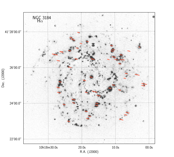
Figure 1.— Continuum-subtracted H$\alpha$ SINGS image of NGC 3184 (Muñoz-Mateos et al., 2009). The footprints of CHAOS slits are overlaid in light red, representing the Field 1, 2, and 3 slit positions observed at the LBT. The slit positions targeted H II regions, although not always centered in order to maximize effective usage of mask real estate and obtain background within the slit. See Table 2 for more details.

2.2. Spectral Reductions

For a detailed description of the data reduction procedures we refer the reader to (B15). Here, we only note the primary points of our data processing. Spectra were reduced and analyzed using the beta-version of the MODS reduction pipeline which runs within the XIDL reduction package. Given that the bright disks of CHAOS galaxies can complicate local sky subtraction, additional sky slits were cut in each mask that provided a basis for clean sky subtraction. Continuum subtraction was performed in each slit by scaling the continuum flux from the sky-slit to the local background continuum level. One-dimensional spectra were then corrected for atmospheric extinction and flux calibrated based on observations of flux standard stars (Bohlin, 2014). At least one flux standard was observed on each night science data were obtained. An example of a flux-calibrated spectrum is shown in Figure 2.

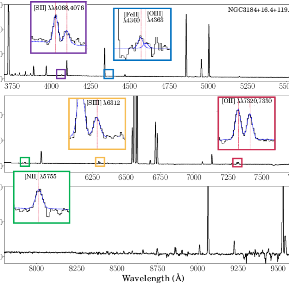
Figure 2.— Demonstration of a one dimensional spectrum taken with MODS1/LBT of region $+16.4+119.8$ in NGC 3184 with auroral line detections at a strength of 3$\sigma$ or greater. The observed spectrum is plotted as a black line, with the model in blue. In the expanded windows, we mark and label the five temperature-sensitive auroral emission line features used in this paper: [S ii] $\lambda\lambda 4068,4076$ [O iii] $\lambda 4636$, [N ii] $\lambda 5755$, [S iii] $\lambda 6312$, and [O ii] $\lambda\lambda 7320,7330$. This spectrum lacks an [O III] $\lambda$4363 detection as the majority of the emission in that region is actually due to a contaminating [Fe II] line at $\lambda$4360 (see blue box). Note that major telluric absorption features are not corrected for (see bottom panel).

2.3. Emission Line Measurements

We provide a more detailed description of the adopted continuum modeling and line fitting procedures applied to the CHAOS observations in B15. Below, we only highlight the fundamental components of this process. We model the underlying continuum of our MODS1 spectra using the STARLIGHT spectral synthesis code (Fernandes et al., 2005) in conjunction with the models of Bruzual & Charlot (2003). Allowing for an additional nebular continuum, we fit each emission line with a Gaussian profile. We note that we have modeled blended lines (H7, H8, and H11 – H14) in the Balmer series based on the measurements of unblended Balmer lines and the tabulated atomic ratios of Hummer & Storey (1987), assuming Case B recombination.

We correct the strength of emission features for line-of-sight reddening using the relative intensities of the four strongest Balmer lines (H$\alpha$/H$\beta$, H$\gamma$/H$\beta$, H$\delta$/H$\beta$). We report the determined values of E(B–V) in Table 4 of Appendix A. We do not apply an ad-hoc correction to account for Balmer absorption as the lines were fit simultaneously with the stellar population models. The stellar models contain stellar absorption with an equivalent width of $\approx$1 – 2 Å in the H$\beta$ line. The uncertainty associated with each measurement is determined from measurements of the spectral variance, extracted from the two-dimensional variance image, uncertainty associated with the flux calibration, Poisson noise in the continuum, read noise, sky noise, flat fielding calibration error, error in continuum placement, and error in the determination of the reddening. We also include a 2% uncertainty based on the precision of the adopted flux calibration standards (Oke, 1990, see discussion in Berg et al. 2015).

A few emission features required extra care, such as the intrinsically faint auroral lines that are critical to this study. As has been done with the previous CHAOS galaxies, we inspected the lines by-eye and measured the flux of each auroral line by-hand in the extracted spectra to confirm the fit. In cases where these measurements were in disagreement, we adopted the by-hand measurement. This was most common for the [N II] $\lambda$5755 line which falls near the wavelength region affected by the dichroic cutoff of MODS and the “red bump” Wolf-Rayet carbon features. Additionally, we have updated our line fitting code to include the [Fe II] $\lambda$4360 emission feature, which may significantly contaminate [O III] $\lambda$4363 line measurements at high metallicities (12+log(O/H) $>$ 8.4; Curti et al., 2017).

Finally, the [O II] $\lambda$$\lambda$3726,3729 doublet is blended for all observations due to the moderate resolution of MODS. However, two components are apparent in the doublet profile for the majority of spectra, and are therefore modeled using two Gaussian profiles. The reported [O II] $\lambda$3727 fluxes represent the total flux in the doublet.

The reddening-corrected emission line intensities measured from H II regions in NGC 628, NGC 5194, and NGC 5457 have been previously reported in B15, C15, and C16, respectively. For the NGC 3184 observations reported here, the reddening-corrected line intensities are listed in Table 4 of Appendix A.

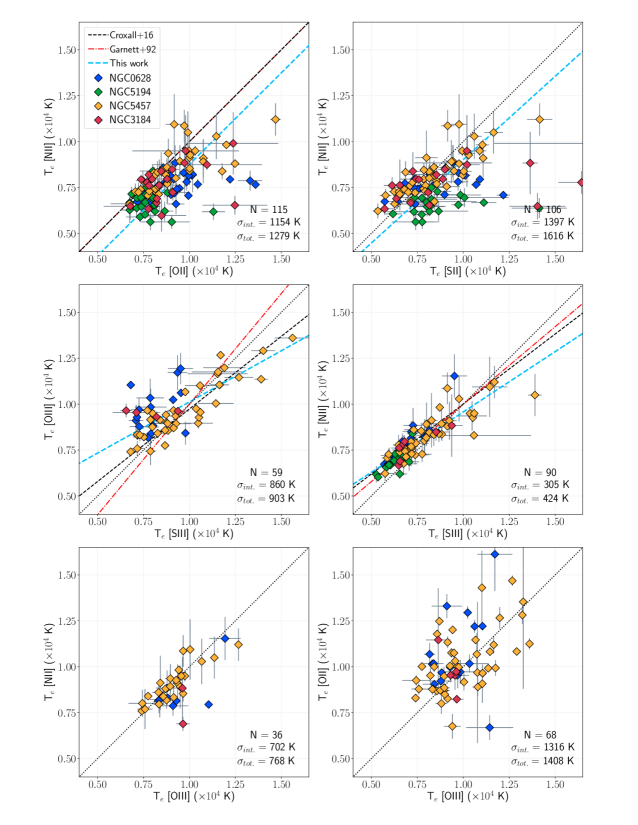
Figure 3.— Comparing temperature relationships for different ions from all four CHAOS galaxies. The black dotted lines assume a one-to-one relationship, red dot-dashed lines are the photoionization model relationships from Garnett (1992), black dashed lines are the updated empirical relationships from C16, and blue dashed lines are the best linear fits to the data from all four CHAOS galaxies. The top panels compare measures of the low-ionization zone temperatures. Top left: $T_{e}$[N II] versus $T_{e}$[O II], showing large scatter, and top right: $T_{e}$[N II] versus $T_{e}$[S II], offset significantly from one-to-one. The middle panels compare to the intermediate-ionization temperature, $T_{e}$[S III], revealing the scattered $T_{e}$[O III] versus $T_{e}$[S III] trend (left) and the tight correlation between T[N II] and T[S III] (right). The bottom panels show further comparisons to the high-ionization temperature, $T_{e}$[O III]. The T[N II] versus T[O III] trend (left) is relatively well behaved, but has few points, whereas T[O II] versus T[O III] (right) is a scatter plot. We adopt the C16 relationships, given in Equations $1-3$, for this work.

3. Direct Gas-Phase Abundances

3.1. Electron Temperature and Density Determinations

The combined sensitivity and large wavelength coverage of CHAOS observations allows electron temperature and density measurements from multiple ions. The temperature-sensitive auroral-to-nebular line ratios most commonly observed in the CHAOS spectra are [S II] $\lambda$$\lambda$4068,4076/$\lambda$$\lambda$6717,6731; [O III] $\lambda$4363/$\lambda$$\lambda$4959,5007; [N II] $\lambda$5755/$\lambda$$\lambda$6548,6584; [S III] $\lambda$6312/$\lambda$9069,9532; and [O II] $\lambda$$\lambda$7320,7330/$\lambda$$\lambda$3727,3729. To account for possible contamination by atmospheric absorption of the red [S III] lines, we follow our practice in B15 of upward correcting the weaker of the two lines by the theoretical ratio of $\lambda$9532/$\lambda$9069 = 2.47. Assuming a three-zone ionization structure, these measurements probe the physical conditions throughout the nebula, and allow for the comparison of multiple measures in the low-ionization zone. We use the ratio of the [S II] $\lambda$$\lambda$6717,6731 emission lines as a sensitive probe of the nebular electron density in typical H II regions ($10^{1.5}<n_{e}({\rm cm}^{-3})<10^{3.5}$). In order to compare the first four CHAOS galaxies in a uniform, consistent manner, we recalculate the nebular temperatures and densities adopting the atomic data reported in Table 4 of B15 and using the observed temperature- and density-sensitive line ratios with the PyNeb package in python (Luridiana et al., 2012, 2015).

3.1.1 Temperature Relationships

It is common practice to use temperature-temperature ($T_{e}-T_{e}$) relationships derived from photoionization models to infer the temperatures in unobserved ionization zones. The relationships of Garnett (1992, hereafter, G92) are a typical choice; however, significant updates in atomic data (especially for [S III] and [O II]; see Figure 4 in B15) have occurred since the time of that work and so new relationships are warranted.

In C16, we obtained temperature measurements from one or more auroral lines in 74 H II regions in M101, the largest number in a single galaxy to date. These data used the updated atomic data recommended in B15, and provided a large dataset of well measured temperatures from multiple ions that allowed us to empirically determine new $T_{e}-T_{e}$ relationships:

$$T_{e}{[\rm{NII}]}=(0.714\pm 0.142)\times T_{e}{[\rm{OIII}]}+(2.57\pm 1.25),$$ (1)

$$T_{e}{[\rm{SIII}]}=(1.312\pm 0.075)\times T_{e}{[\rm{NII}]}-(3.13\pm 0.58),$$ (2)

$$T_{e}{[\rm{SIII}]}=(1.265\pm 0.140)\times T_{e}{[\rm{OIII}]}-(2.32\pm 1.35),$$ (3)

where temperatures are in units of $10^{4}$ K.

Using the combined data from the first four CHAOS galaxies, we compile a sample of 190 individual H II regions with multiple auroral line measurements. Of these regions, 175 have $T_{e}$[O III], $T_{e}$[S III], or $T_{e}$[N II]. In Figure 3 we compare these data to the $T_{e}-T_{e}$ relationships of G92 (red dot-dashed lines) and C16 (black dashed lines). For reference, the line of equality is shown as a dotted black line. We recognize that these are simple $T_{e}-T_{e}$ relationships; in the future we will use the full CHAOS dataset to explore more complicated $T_{e}-T_{e}$ relationships, for example, accounting for the effects of ionization discussed below.

For each set of variables, we determine the best fit $T_{e}-T_{e}$ relationship using a Bayesian linear regression. Specifically, we use the code python linmix, which is an implementation of the linear mixture model algorithm developed by Kelly (2007) to fit data with uncertainties on two variables, including explicit treatment of intrinsic scatter. Intrinsic scatter, $\sigma_{int.}$, is due to real deviations in the physical properties of our sources that are not completely captured by the variables considered. By introducing an additional term representing the intrinsic scatter to the weighting of each data point in the fit, we can determine the median of the normally-distributed intrinsic random scatter about the regression. The calculated total and intrinsic scatters, $\sigma_{tot.}$ and $\sigma_{int.}$ respectively, as well as the number of regions used in the fit, are presented in Figure 3.

The top two panels of Figure 3 compare temperature measurements that characterize the low-ionization zone. On the left, we use the 115 regions with both [N II] and [O II] measurements in our sample, and find a best fit of $T_{e}$[N II]$=[T_{e}$[O II]$-(1.203\pm 1.144)]/(1.004\pm 0.150)$. As expected, the overall trend follows a one-to-one relationship within the limits of the uncertainties, but with both large total ($\sigma_{tot.}=1280$ K) and intrinsic ($\sigma_{int.}=1150$ K) scatters. While equal temperatures are expected from photoionization models, the data tend to be shifted toward higher $T_{e}$[O II]. This is true for the majority of the sample, which is clustered within $1000-2000$ K of the equality relationship, but especially for the more extreme outliers that offset up to roughly 5000 K.

We note that dielectronic recombination can contribute to the observed [O II] emission, especially $\lambda$$\lambda$7320,7330, in more metal-rich nebulae (e.g., Rubin, 1986). The magnitude of the effect increases strongly with decreasing temperature (increasing metallicity) but depends on the electron density. To this end, Liu et al. (2001) showed that recombination can play an important role in exciting both the [O II] $\lambda$$\lambda$7320,7330 and [N II] $\lambda$5754 auroral lines in the higher-density gas of planetary nebulae ($>10^{3}$ cm^-3). These authors showed that this effect leads to overestimated [O II]- and [N II]-derived electron temperature measurements. However, we show below that $T_{e}$[N II] is well behaved with respect to $T_{e}$[S III] which implies that the recombination contribution must be small at the low densities of our nebulae. Thus our data are consistent with previous reports of systematically larger $T_{e}$[O II] than $T_{e}$[N II] measurements (e.g., Esteban et al., 2009; Pilyugin et al., 2009; Berg et al., 2015) that cannot be accounted for by recombination processes, and so we do not favor [O II] as a reliable low-ionization zone temperature indicator. We reserve further analysis for the complete CHAOS sample, where we will revisit the reliability of [O II] as a diagnostic and investigate the effects of sky contamination, recombination, and reddening.

In the top right panel of Figure 3, we compare [N II] and [S II] using the [S II] temperatures presented in C16, plus newly derived values for NGC 628, NGC 5194, and NGC 3184, comprising a sample of 106 regions. As expected for two ions that probe similar low-ionization gas, the best fit is consistent with equality as $T_{e}$[N II]$=[T_{e}$[S II]$-(0.072\pm 1.392)]/(1.101\pm 0.180)$. Again, the intrinsic scatter accounts for the majority of the total scatter; however, the large deviations observed indicate that observational uncertainties still play a large role at high [S II] temperatures.

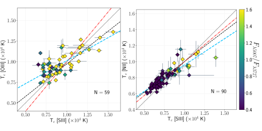
Figure 4.— $T_{e}$[O III] versus $T_{e}$[S III] (left) and $T_{e}$[N II] versus $T_{e}$[S III] (right) for all four CHAOS galaxies color-coded by the reddening-corrected [O III] $\lambda$5007/[O II] $\lambda$3727 flux ratios. The tight correlation between $T_{e}$[N II] and $T_{e}$[S III] seen for the dark blue / purple points promotes the use of these low- and intermediate-ionization zone temperatures for low-ionization H II regions (low $F_{\lambda 5007}$/$F_{\lambda 3727}$). However, comparing the high-ionization yellow points in the two plots suggests it is better to use the high-ionization zone temperature, $T_{e}$[O III], for H II regions with high $F_{\lambda 5007}$/$F_{\lambda 3727}$.

In the middle two panels of Figure 3, we examine the relationship between the intermediate-ionization zone, characterized by [S III], with both the high-ionization zone ([O III]; left) and low-ionization zone ([N II]; right). In the middle left panel, we find the best fit to the $T_{e}$[O III]$-T_{e}$[S III] relationship is in good agreement with C16, but diverges from G92 for the hottest regions observed: $T_{e}$[S III] $=(1.795\pm 0.067)\times T_{e}$[O III] $-(8.167\pm 1.122)$. Previous studies have reported large discrepancies between $T_{e}$[O III] and $T_{e}$[S III] and significant scatter in their relationship (e.g., Hägele et al., 2006; Pérez-Montero et al., 2006; Binette et al., 2012; Berg et al., 2015). The $T_{e}$[O III]$-T_{e}$[S III] relationship for our sample of 59 regions is no exception, with a significant scatter of $\sigma_{tot.}=900$ K that can be attributed almost entirely to intrinsic scatter ($\sigma_{int.}=860$ K). Given the large number of outliers presented in both our sample and the literature, we reiterate and stress the finding of B15 that $T_{e}$[O III] alone is less reliable than $T_{e}$[S III] or $T_{e}$[N II] for abundance calculations in metal-rich H II regions.

Curti et al. (2017) cautioned of the potential contamination of the temperature-sensitive [O III] $\lambda$4363 line by the neighboring [Fe II] $\lambda$4360 line. This effect is especially prominent at abundances of 12+log(O/H)$>8.4$, where the [Fe II] line increases in strength and the [O III] $\lambda$4363 line becomes faint due to the decreasing H II region temperature. Because Curti et al. (2017) study used stacks of integrated galaxy light spectra in their study, the source of the [Fe II] $\lambda$4360 emission is difficult to trace; however, as a precaution we have added the Fe II emission feature to our line fitting code so that the [Fe II] $\lambda$4360 and [O III] $\lambda$4363 lines are simultaneously fit and deblended, and have inspected the fits by-eye (see § 2.2). In fact, we do not measure $T_{e}$[O III] in any very metal rich H II regions in CHAOS and so do not find any significant [Fe II] contamination affecting our $T_{e}$[O III] measurements. For instance, [Fe II] $\lambda$4360 emission is seen in the blue inset window of the spectrum shown in Figure 2. However, [O III] $\lambda$4363 was not strong enough to be identified as a detection and so the high-ionization zone temperature was inferred from $T_{e}$[S III] and not affected by the [Fe II] contamination.

In the middle right panel of Figure 3 we plot $T_{e}$[N II] versus $T_{e}$[S III]. Similar to the trend reported in B15, we find a very tight correlation, especially for the coolest, most metal-rich regions typical of CHAOS (with $T_{e}<10^{4}$ K). The best fit line (blue) to the 90 regions is $T_{e}$[S III] $=~{}(1.522\pm 0.042)\times~{}T_{e}$[N II]$-(4.576\pm 0.463)$, in agreement with the relationship of C16 (black dashed line) and about which the dispersion is quite small: $\sigma_{tot.}=420$ K. The C16 relationship is also very similar to the G92 relationship, where differences (seen in both bottom panels) are likely due to changes in the adopted [S III] atomic data.

Finally, we compare the low- and high-ionization zones in the bottom two panels of Figure 3. On the left, the relationship between the low-ionization zone $T_{e}$[N II] and the high-ionization zone $T_{e}$[O III] is reasonably well behaved, but has too few data points to analyze further. On the other hand, the $T_{e}$[O II]$-T_{e}$[O III] plot shows a cloud of scattered points that is difficult to characterize.

Significant [O III] $\lambda$4363, [N II] $\lambda$5755, and/or [S III] $\lambda$6312 detections are measured in 30 regions in NGC 3184, resulting in direct oxygen abundance measurements. The electron temperatures and densities characterizing each H II region observed in NGC 3184 are reported in Table 5 in Appendix A.

3.1.2 Ionization-Based Temperature Priorities

CHAOS has proven highly successful at measuring significant detections of both [N II] $\lambda$5755 and [S III] $\lambda$6312, demonstrating the utility of these lines in metal-rich H II regions. Given the robust $T_{e}$[N II]$-T_{e}$[S III] relationship demonstrated for the 90 H II regions with simultaneous detections, our results further endorse the recommendation of B15 to prioritize these two temperature indicators. However, it is interesting that the $T_{e}$[N II]$-T_{e}$[S III] relation shows a notable increase in dispersion for $T_{e}>10^{4}$ K, whereas the dispersion in the $T_{e}$[O III]$-T_{e}$[S III] relationship seems to settle down in that same $T_{e}$ regime.

Recently, Yates et al. (2019) measured a large range of $T_{e}$[O III]/$T_{e}$[O II] ratios spanning significant temperature (and, due to its inverse dependence, metallicity) parameter space from a sample of 130 H II regions and integrated-light galaxies. They postulate that deviations from equal temperatures are rooted in the ionization structure of the nebulae, where O⁺⁺-dominated nebulae have cooler [O III] temperatures and O⁺-dominated nebulae have cooler [O II] temperatures. Because the relative flux of the [O III] $\lambda$5007 and [O II] $\lambda$3727 emission lines are dependent on the number of oxygen ions in the O⁺⁺ relative to O⁺ state, we can use the [O III] $\lambda$5007/[O II] $\lambda$3727 ratio as a proxy for O⁺⁺/O⁺, or the ionization structure.

In Figure 4 we reproduce the $T_{e}$[O III]$-T_{e}$[S III] and $T_{e}$[N II]$-T_{e}$[S III] relationships from Figure 3, but with the points color-coded by their reddening-corrected [O III] $\lambda$5007/[O II] $\lambda$3727 flux ratios. As expected, low ionization H II regions (low $F_{\lambda 5007}$/$F_{\lambda 3727}$; dark blue/purple points) show the tightest correlation between the low- and intermediate-ionization zone temperatures ($T_{e}$[N II] versus $T_{e}$[S III]) and high ionization H II regions (high $F_{\lambda 5007}$/$F_{\lambda 3727}$; yellow points) show the tightest correlation between high- and intermediate- ionization zone temperatures ($T_{e}$[O III] versus $T_{e}$[S III]). Motivated by these dispersion-ionization correlations, we recommend simple, yet improved, ionization-based temperature priorities below.

While few $T_{e}$[O III] detections were found in the first CHAOS paper examining NGC 628, many more detections were added with the addition of NGC 5457, revealing the utility of $T_{e}$[O III] at high $T_{e}$ and high ionization (high $F_{\lambda 5007}$/$F_{\lambda 3727}$). Therefore, we prefer a $T_{e}$[O III] measurement for high ionization nebulae that are dominated by the O⁺⁺ zone and a $T_{e}$[N II] measurement for low ionization nebulae that are predominantly O⁺, where $T_{e}$[S III] is used in the absence of a [N II] $\lambda$5755 detection. In order to apply this rubric, we define a high (low) ionization nebula criteria of $F_{\lambda 5007}$/$F_{\lambda 3727}>$ ($<$) 1.25. This division was chosen based on a statistical analysis of the $T_{e}$[O III]-based oxygen abundance dispersion with $F_{\lambda 5007}$/$F_{\lambda 3727}$ using data from the C16 study of M101 and the Rosolowsky & Simon (2008) study of M33, where dispersion was minimized for $F_{\lambda 5007}$/$F_{\lambda 3727}>1.25$. The details of this analysis will be presented in Berg et al. (2020).

3.2. Abundance Determinations

We calculate absolute and relative abundances using the PyNeb package in python, assuming a five-level atom model (De Robertis et al., 1987), the atomic data reported in Table 4 of B15, and the temperatures determined from the [O III], [S III], and/or [N II] measured temperatures in conjunction with $T_{e}-T_{e}$ scaling relationships. We showed in Section 3.1 that our electron temperature results for the first four CHAOS galaxies are consistent with the C16 $T_{e}-T_{e}$ relationships, therefore, we use Equations $1-3$ to determine the temperatures of unmeasured ionization zones. Further, the dispersion in our measured $T_{e}-T_{e}$ relationships correlates with the average ionization of the nebulae, as represented by the $O_{32}=F_{\lambda 5007}/F_{\lambda 3727}$ ratio.

We adopt the ionization-based temperature prioritization depicted in Figure 5. Specifically, if all three ionic temperatures are measured and the average ionization of the nebula is relatively high ($O_{32}>1.25$), we prioritize $T_{e}$[N II] for the low-ionization zone, $T_{e}$[S III] for the intermediate-ionization zone, and $T_{e}$[O III] for the high-ionization zone. If instead the average ionization of the H II region is relatively low ($O_{32}<1.25$), we adopt the measured low- and intermediate-ionization zone temperatures as before, but instead use $T_{e}$[S III] in combination with Eqn. 3 to infer the high-ionization zone temperature. The justification of this choice is the large dispersions for high-ionization points in the $T_{e}-T_{e}$ relations shown in Figure 4, with the result that we have less confidence in $\lambda$4363 in this regime (see discussion in § 4.2). In the absence of a measurement of the appropriate ionization-zone temperature, temperatures should be inferred from the next preferred ion measured (following the ordering in Figure 5) in combination with the $T_{e}-T_{e}$ relationships from Equations $1-3$.

While the ionization-based temperature prioritizations presented here offer an improvement to temperature-based abundance determinations, we note two caveats. First, it is best to have independent measurements of the temperature in each ionization zone to reduce the reliability on relationships from photoionization modeling. Second, there are inherent, systematic uncertainties remaining due to the nominal assumption that H II region structures can be simply divided into three 1D ionization zones when the reality is much more complicated.

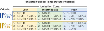
Figure 5.— Updated temperature prioritization for different ionization zones from the CHAOS data. The priorities are to be used to select the first measured ion temperature from each ordered list and are split into two separate decision trees based on the $O_{32}=F_{\lambda 5007}/F_{\lambda 3727}$ ratio, which is used to determine the average ionization of an H II region.

3.2.1 Oxygen Abundances

We adopt the ionization-based temperature prioritization recommended in Figure 5 in order to determine the abundances of the first four CHAOS galaxies in a uniform, homogeneous manner. Ionic abundances relative to hydrogen are calculated using:

$$\frac{N(X^{i})}{N(\rm{H}^{+})}=\frac{I_{\lambda(i)}}{I_{\rm{H}\beta}}\frac{j_{\rm{H}\beta}}{j_{\lambda(i)}},$$ (4)

where the emissivity coefficient, $j_{\lambda(i)}$, is sensitive to the adopted temperature.

The total oxygen abundance is calculated as the sum of the O⁺/H⁺ and O⁺⁺/H⁺ ion fractions. While emission from O⁺³ is negligible in typical star-forming regions, some oxygen might be in O⁰ phase for the moderate-to-low ionization parameters characteristic of the CHAOS data ($-2.5<$ log $U<-4.0$; see, for example, Figure 5 in Berg et al., 2019). In the current work, we can estimate the typical contribution to the oxygen abundance by O⁰ emission using the [O I] $\lambda$6300 feature, which can be distinguished from the [O I] $\lambda$6300 night sky line at the distances of our sample and the resolution of MODS. For our sample, the average $I$([O I]$\lambda$6300)/$I$(H$\beta)=0.022$, corresponding to an O⁰/(O${}^{0}+$O${}^{+}+$O⁺⁺) fraction of 3%. This means that, on average, the oxygen abundance may be underestimated by only $\Delta$O/H$<0.02$ dex due to missing O⁰/H⁺ contributes. Given that possible contributions from O⁰ are typically less significant than the uncertainties on the oxygen abundance measurements, O⁰/H⁺ is not included in our oxygen abundance determinations, consistent with previously published CHAOS data.

The total oxygen abundances for our NGC 3184 sample are reported in Table 5 of Appendix A, noting that neither O⁰ nor contributions from dust (also typically $<0.1$ dex; Peimbert & Peimbert, 2010; Peña-Guerrero et al., 2012) are included. Additionally, given that the abundances reported in previous CHAOS works were not derived with methodology consistent with Figure 5, we re-derive the abundances for NGC 628, NGC 5194, and NGC 5457 in order to compare our sample in a uniform manner. Since both NGC 628 and NGC 5194 were analyzed following the methodology laid out in B15 and both had very few [O III] $\lambda$4363 detections, their results were not significantly modified. C16’s study of NGC 5457, on the other hand, generally prioritized [O III]-derived temperatures for the purpose of comparing to $T_{e}$[O III]-based abundances in the literature. The total and relative abundances for NGC 628, NGC 5194, and NGC 5457 used in this work are report in Table 6 in Appendix  B.

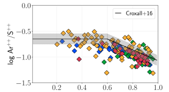
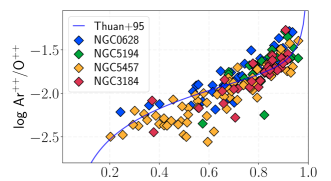
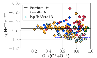
Figure 6.— Three of the ionization correction factors considered in this work versus low-ionization fraction of oxygen, O$+$/(O${}^{+}+$O⁺⁺). In the top panel, we plot the Ar⁺⁺/S⁺⁺ ICF relationship introduced by C16. We note that NGC 3184 seems to deviate from the relationship to lower Ar⁺⁺/S⁺⁺ values with decreasing ionization. In the middle panel, we plot the Ar⁺⁺/O⁺⁺ ratio and corresponding ICF(Ar) from Thuan et al. (1995). The NGC 3184 observations align well with this relationship. In the bottom panel, we plot the Ne⁺⁺/O⁺⁺ ratio, revealing two populations at low ionization (see also C16). We also consider regions with low log(Ne/Ar) ratios ($<1.3$; light blue circles), which largely correspond to the low Ne⁺⁺/O⁺⁺ points.

3.2.2 Nitrogen Abundances

We also observe significant N, S, Ar, and Ne emission lines in our spectra that allow us to determine their relative abundances. However, when emission lines from prominent ionization stages are absent in the optical, their abundance determinations require an ionization correction factor (ICF) to account for the unobserved ionic species. For nitrogen, we employ the common assumption that N/O = N⁺/O⁺, such that the ICF(N) = (O⁺ $+$ O⁺⁺)/O⁺ (Peimbert, 1967). While the O⁺ ionization zone overlaps both N⁺ and N⁺⁺, N/O = N⁺/O⁺ benefits from comparing two ions in the same temperature zone, and Nava et al. (2006) found this assumption valid within a precision of roughly 10%. We report the ionic, total, and relative N abundances for NGC 3184 in Table 5 in Appendix A. We also list the ICF, where the uncertainty is solely a propagation of the emission line uncertainties.

3.2.3 Sulfur Abundances

For sulfur, both S⁺ (10.36–22.34 ev) and S⁺⁺ (22.34–34.79 eV) span the O⁺ zone (13.62–35.12 eV), as the transitions from S⁺⁺ to S⁺³ and O⁺ to O⁺⁺ are nearly coincident. We note that the low ionization energy of S⁺ means that [S II] emission can originate from outside the H II regions ($E\leq 13.59$ eV), and, therefore, caution must be used when interpreting these lines. While we do not currently correct for such diffuse ionized gas in CHAOS, the high-ionization of our nebulae ensure that the this gas only constitutes a small fraction.

In high-ionization nebulae, S⁺³ (34.79–47.22 eV) lies in the O⁺⁺ zone (35.12–54.94 ev). To account for the unseen S⁺³ ionization state we employ the ICF from Thuan et al. (1995) for high-ionization H II regions characterized for O⁺/O$\leq 0.4$, where the total O is assumed to be O = O${}^{+}+$O⁺⁺. However, because the metal-rich H II regions of CHAOS are typically cooler and moderate-ionization, we follow the recommendation of C16 and adopt ICF(S) = O/O⁺⁺ (or simply S/O = (S${}^{+}+$S⁺⁺)/O⁺) for O⁺/O$>0.4$ (see, also, Peimbert & Costero, 1969). The resulting ICFs and ionic, total, and relative S abundances for NGC 3184 are tabulated in Table 5 in Appendix A. The uncertainty on the ICF(S) is a propagation of the emission line uncertainties for O⁺/O$>0.4$ and 10% of the ICF(S) in the case of O⁺/O$\leq 0.4$ (see Thuan et al., 1995).

3.2.4 Argon Abundances

In the case of argon, only the Ar⁺⁺ ionization state is observed in the majority of CHAOS optical spectra, but the ionization potentials of O⁺ (13.62–35.12 eV) and O⁺⁺ (35.12–54.94 ev) encompass portions of Ar⁺ (15.76–27.63 eV), Ar⁺⁺ (27.63–40.74 eV), and Ar⁺³ (40.74–59.81 eV). While ratios of sulfur and oxygen ions relative to Ar⁺⁺ have both been used individually in the past to trace unseen argon ions, C16 found that the low-ionization regions of the CHAOS NGC 5457 sample are not well represented by either. Instead, C16 corrected for the decrease in Ar⁺⁺/S⁺⁺ seen in low-ionization nebula by adopting a linear correction to Ar⁺⁺/S⁺⁺: log(Ar⁺⁺/S${}^{++})=-1.049\times$(O⁺/O)$-0.022$, for O⁺/O $\geq 0.6$. For higher ionization nebulae, Ar⁺⁺/S⁺⁺ was uncorrelated with O⁺/O and so a constant value of log(Ar⁺⁺/S${}^{++})=-0.65$ was assumed, similar to Kennicutt et al. (2003b).

The log(Ar⁺⁺/S⁺⁺) correction from C16 is shown in the top panel of Figure 6. The previously reported trend of decreasing Ar⁺⁺/S⁺⁺ with increasing O⁺/O is reproduced, but with more dispersion in the updated ionic abundances, especially for NGC 5457 – the data it was derived for. We find that all four CHAOS galaxies follow just as well the Ar⁺⁺/O⁺⁺-based ICF of Thuan et al. (1995) over the full range in O⁺/O probed by the sample. Given that three of the galaxies seem to be systematically offset from the Ar⁺⁺/S⁺⁺ relation, we choose to apply the ICF(Ar) from Thuan et al. (1995), which has an uncertainty of 10%, to all four CHAOS galaxies. The differences between the updated ion fractions and those measured in C16 support the finding by Yates et al. (2019) and this work that ionization plays an important role in the temperature and metallicity determinations of an H II region. We list the resulting Ar abundances in Table 5 of Appendix A.

3.2.5 Neon Abundances

Neon is similar to argon in that only one ionization state is typically observed, Ne⁺⁺ (40.96–63.45 eV). Therefore, we use the ICF suggested by Peimbert & Costero (1969) and Crockett et al. (2006) to correct for the unobserved Ne⁺ ions (21.57–40.96 eV): ICF(Ne) = O/O⁺⁺, where standard propagation of errors is used to determine the uncertainty. Then, Ne/O = Ne⁺⁺/O⁺⁺. Just as C16 reported a bifurcation in the Ne⁺⁺/O⁺⁺ values of NGC 5457, we see a similar downward dispersion for low ionization (O⁺/O $>0.5$) in the bottom panel of Figure 6 for our four-galaxy sample (see, also, Kennicutt et al., 2003a). Interestingly, we also note an upturn to high Ne⁺⁺/O⁺⁺ values for some low-ionization nebulae.

The unseen Ne⁺ (21.56–40.96 eV) partially overlaps with both the O⁺ and O⁺⁺ ionization zones. This means that a significant fraction of Ne likely lies in the Ne⁺ state, especially for the moderate-ionization nebulae observed by CHAOS. This results in underestimated total Ne abundances in low- to moderate-ionization nebulae, a well-known issue with the classical ICF(Ne) (Torres-Peimbert & Peimbert, 1977; Peimbert et al., 1992). García-Rojas et al. (2013) observed a similar trend in the Ne/Ar ratios of planetary nebulae, where low-ionization targets appeared Ne-poor and Ar-rich. Interestingly, many of the low Ne⁺⁺/O⁺⁺ CHAOS points also exhibit the lowest values of log(Ar/Ne), which are plotted as light blue circles in Figure 6.

Using the average Ar/Ne ratio of the CHAOS sample as a guide, we apply a Ne/Ar correction that is normalized to the average value for low-ionization regions (O⁺/O $>0.5$) and update the Ne/O values (see Section 6.1). Overall, this correction seems to pull the regions with low-ionization Ne/O abundances up, while regions with suspiciously low Ar/O abundances in NGC 5457 are adversely affected. The resulting Ne abundances are reported in Table 5 of Appendix A. While this updated ICF(Ne) is clearly not perfect, these relationships are illuminating and suggest that a more sophisticated ICF is needed to fully correct the total Ne abundance. A more in depth discussion of the analysis of the CHAOS ICFs can be found in C16.

4. Radial Abundance Trends

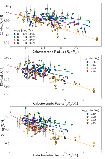
Figure 7.— Abundance trends plotted vs. galactocentric radius for the first four CHAOS galaxies: the O/H gradient normalized to the $R_{25}$ radius of each galaxy (top), the O/H gradient normalized to each galaxy’s effective radius, $R_{e}$ (middle), and the S/H gradient normalized to $R_{e}$ (bottom). We note that the O/H gradients appear to be no more ordered when plotted relative to $R_{e}$, as originally proposed by Sánchez et al. (2014), as they show individual differences in their slopes and dispersions regardless of the radial normalization. Interestingly, S/H gradients show a similar ordering as O/H. See Table 1 for properties of the CHAOS galaxies.

4.1. Radial Oxygen Abundance Gradients

In the past, studies of radial abundance trends have used both a variety of methods to characterize abundance and to normalize the galactocentric radius to show significant variations in the gradients of different galaxies (e.g., Zaritsky et al., 1994; Moustakas et al., 2010). However, many of these studies have relied on abundance measurements in just a handful of H II regions per galaxy. More recently, abundance trends have been studied in large numbers of H II regions using integral field unit (IFU) spectroscopy of individual galaxies. Using empirical oxygen abundances determined from CALIFA IFU spectra, Sánchez et al. (2014) found a universal O/H gradient with a characteristic slope of $\alpha_{\rm O/H}=-0.10\pm 0.09$ dex$/R_{e}$ over $0.3<R_{g}/R_{e}<2.0$ for 306 galaxies, whereas Sánchez-Menguiano et al. (2016) report a shallower slope of $\alpha_{\rm O/H}=-0.075$ dex$/R_{e}$, with $\sigma=0.016$ dex for 122 face-on spiral galaxies. However, the recent study of 102 spiral galaxies using VLT/MUSE IFU spectra by (Sánchez-Menguiano et al., 2018) found a distribution of slopes with an average of $\alpha_{\rm O/H}=-0.10\pm 0.03$ dex$/R_{e}$. These authors find that radial gradients are steepest when the presence of an inner drop or an outer flattening is also detected in the radial profile, and point to radial motions in shaping the abundance profiles.

While IFU studies have greatly expanded our understanding of abundance gradients, they have thus far relied on strong-line abundance calibrations, and therefore have systematic uncertainties (e.g., see reviews from Kewley & Ellison, 2008; Maiolino & Mannucci, 2019). CHAOS now allows us to compare radial abundance trends using large numbers of direct abundance measurements in H II regions. We display the O/H abundances derived in Section 3.2.1 for the four CHAOS galaxies in Figure 7 as a function of galactocentric radius. Because the locations of individual H II regions are known with high precision relative to one another, we consider only the uncertainties associated with oxygen abundance here. We plot the galactocentric radius relative to the isophotal ($R_{25}$) and effective ($R_{e}$) radii of each galaxy in the top and middle panels of Figure 7, respectively. Because there is no visual evidence for an outer-disk flattening in the O/H gradient in the coverage of the CHAOS sample, we characterize the O/H gradient in each galaxy with a single, Bayesian linear regression using the python linmix code (solid lines). Parameters of the resulting fits are given in Table 2.

Comparing the individual O/H gradients in Figure 7, there are apparent differences in both the O/H versus $R_{g}/R_{25}$ and O/H versus $R_{g}/R_{e}$ gradients in the top and middle panels, respectively. While the gradients align more closely when plotted versus the effective radius ($R_{e}$), the gradients of individual galaxies are still uniquely distinct. The four CHAOS galaxies have a range of slopes of $-0.20<\alpha_{\rm O/H}$ (dex$/R_{e}$) $<-0.07$. Because the high-quality direct abundances of the CHAOS sample allow us to better constrain the unique gradient of an individual galaxy, we are seeing tangible gradient differences, even amongst just 4 galaxies, but within the dispersion seen for the large CALIFA samples of strong-line abundances. In this sense, the CHAOS data are demonstrating that O/H versus $R_{g}/R_{e}$ gradients are not uniformly behaved.

NGC 5194 presents the largest deviation from the typical CHAOS slope, where its nearly flat slope has been attributed to interactions with its companion, NGC 5195, resulting in radial migration and mixing of the interstellar gas (see discussion in C15, ). However, even when we only consider the three non-interacting spiral galaxies in our sample, we find tangible differences in the O/H abundance gradients and dispersions of individual CHAOS galaxies. The varying coefficients of the best-fit gradients characterizing the CHAOS galaxies (tabulated in Table 2) show that detailed direct abundance measurements reveal a range in the chemical evolution of individual galaxies.

4.2. Radial Sulfur Abundance Gradients

Sulfur abundances can be an extremely useful tool, particularly in the absence of oxygen abundance information. Notably, sulfur abundances only require a limited wavelength coverage of $\sim$$\lambda$4850–$\lambda$9100 (but better if coverage extends to $\sim$$\lambda$9600) to ensure measurement of all the necessary inputs to a direct abundance: (i) reddening correction (from H$\alpha$/H$\beta$ and the Paschen lines), (ii) density (from [S II] $\lambda$6717/$\lambda$6731), (iii) temperature (from [S III] $\lambda$6312/$\lambda$9069), (iv) S⁺ (from [S II] $\lambda$$\lambda$6717,6731), and (v) S⁺⁺ (from [S III] $\lambda$$\lambda$9069,9532). Surveys with limited blue wavelength coverage (e.g., MUSE; Bacon et al., 2010) may therefore be able to take advantage sulfur’s utility and measure direct abundance trends in the absence of the blue oxygen lines.

Prompted by the importance of S as a temperature indicator, and the expectation of alpha-elements that S and O abundances should trace one another, we explore the S/H gradients of the CHAOS galaxies in the bottom panel of Figure 7. As before, we fit Bayesian linear regression models and report the results in Table 2. The S/H and O/H gradients of our galaxies are all consistent within the uncertainties, with the interesting exception of NGC 628. These fits suggest that S/H abundances provide an alternative direct measurement of a galaxy’s metallicity gradient. S/H abundances may also be easier to measure in moderate- to metal-rich H II regions where [S III] $\lambda$6312 is significantly detected more often than [O III] $\lambda$4363. However, it is important to note that S/H abundances have the disadvantage of requiring an ICF for the unseen S⁺³ and thus, are generally considered inferior to O/H abundances. Typically, in the CHAOS sample, the correction for S⁺³ is less than 20%, but it can get as high as 80%, so caution is warranted.

Why does sulfur seem to behave so well for the CHAOS sample? While the dominant observable ionic states of O in the CHAOS spectra, O⁺ and O⁺⁺, probe the full ionization range of H II region nebulae, our data largely consist of moderate-ionization nebulae. Our regions have O⁺/O ionization fractions that are typical of the more metal-rich H II regions in spiral galaxies, and this combination produces regions that are both more moderate ionization and have cooler temperatures. Given this, it is perhaps not surprising that $T_{e}$[S III] characterizes the CHAOS data so well. At the typically higher metallicities of the CHAOS regions, the nebula are generally lower-excitation and so have large S⁺⁺ fractions (i.e., S⁺⁺ is the dominant ionization zone). To be quantitative, given the excitation energy of [S III] $\lambda$6312 (3.37 eV), a temperature of $T_{e}\sim 7000$ K is required for 1% of the electrons to excite [S III]. This temperature is well matched to the majority of our H II regions, which have temperature measurements of $6000$ K$<T_{e}<8000$ K. On the other hand, the excitation energy of [O III] $\lambda$4363 (5.35 eV) requires a much hotter nebular temperature of $T_{e}\sim 11000$ K for 1% of electrons to excite [O III]. In these typically moderate-ionization nebula, not only is O⁺⁺ a sub-dominant ion, but the relatively low electron temperature of the gas will rarely excite to the upper level of O⁺⁺ from which $\lambda$4363 is emitted. In contrast, the observable ionic states of S in the CHAOS spectra (S⁺, S⁺⁺) probe the lower ionization zones ($\lesssim 35$ eV) that are dominant in the majority of metal-rich H II regions.

4.3. Radial N/O Abundance Gradients:
A Universal N/O Relationship

The N/O abundances for the four CHAOS galaxies are presented in Figure 8. Galactocentric radii are normalized to the isophotal radius, $R_{25}$, of each galaxy in the top panel and to the effective radius, $R_{e}$, in the bottom panel. Once again we analyze gradients of galaxies by comparing their individual Bayesian linear regression fits (solid lines). Interestingly, when trends in N/O versus $R_{g}/R_{25}$ are considered as a single, linear relationship as was done with O/H in Section 4.2, all four galaxies appear to have similar gradients, only offset from one another. Additionally, as noted in previous CHAOS papers, the N/O relationships are more tightly ordered with radius than the O/H gradients, presented by smaller dispersions. On the other hand, when the N/O trends are normalized by their effective radius (bottom panel), three of the four galaxies (NGC 628, NGC 5457, and NGC 3184) shift to lie nearly on top of one another, while NGC 5194 emerges as an outlier once again.

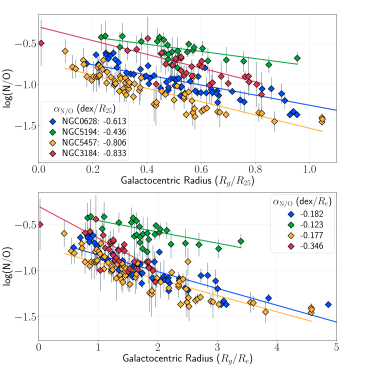
Figure 8.— N/O abundance plotted vs. galactocentric radius for CHAOS galaxy sample presented here. Top: similar to Figure 6, the N/O trend is normalized to the $R_{25}$ radius for each galaxy. Bottom: the N/O gradient relative to effective radius, $R_{e}$. NGC 5194 appears as a clear outlier when plotted in this way.

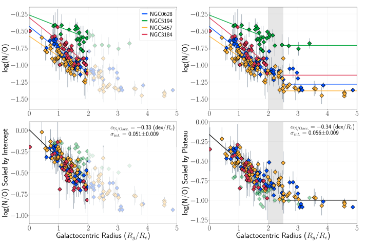
Figure 9.— Top left: N/O versus galactocentric radius of the CHAOS sample with separate fits to N/O for inner disks ($R_{e}/R_{g}<2.0$). Bottom left: N/O trends of each galaxy are offset by the y-intercept of their fits above, producing a remarkably tight N/O gradient for the three non-interacting galaxies. Top right: Considering the full gradient, data in the outer disk ($R_{e}/R_{g}>2.5$) appears to form a flatter trend and so we shade the potential transition grey. As an illustrative exercise, a variance-weighted average plateau is fit for $R_{e}/R_{g}>2.5$ for each galaxy (and assumed for NGC 3184 based on the extrapolated fit for $R_{g}/R_{e}<2.25$). Bottom right: N/O trends are normalized by the average outer disk N/O value of each galaxy, again revealing a universal N/O gradient for $R_{e}/R_{g}<2.0$. If these trends are physical, then the outer flat trend may be the primary N plateau set by the galaxy’s SFH and the inner gradient a primary$+$secondary N trend that transitions near $2.0<R_{e}/R_{g}<2.5$. Data sets with larger radial coverage are needed to test this prediction.

We further investigate the similarities of the CHAOS N/O gradients by comparing them over the same radial extent. Limited by the coverage of NGC 3184, we refit the N/O gradient of the $R_{g}/R_{e}<2.0$ inner disks of the CHAOS galaxies with a Bayesian linear regression model and plot them as solid lines in the top left-hand panel of Figure 9. Now, three of the four galaxies have trends that run parallel to one another: all have very tight trends with slopes of $\alpha_{\rm N/O}=-0.3$ dex/$R_{e}$ and dispersions of $\sigma<0.06$ dex (see Table 2). Given that the inner disk radial gradients decline more steeply for N/O than O/H, these trends are indicative of secondary nitrogen.

In order to isolate the secondary N/O trend of the CHAOS sample, we remove the offset between galaxies by subtracting their individual y-intercept offsets. The resulting scaled N/O versus O/H relationships are shown in the bottom left-hand panel of Figure 9, where a tight secondary N/O relationship emerges that characterizes the entire CHAOS sample well. Given the relatively flat gradient of NGC 5194 in the top left-hand panel of Figure 9, we fit the secondary N/O relationship excluding NGC 5194 (denoted by the semi-transparent green points) in the bottom left-hand panel of Figure 9. The Bayesian linear regression reports a slope of $\alpha_{\rm N/O}=-0.33$ dex/$R_{e}$, with a very small total dispersion of $\sigma=0.08$ dex.

It is remarkable that a simple shift produces such a tight secondary N/O gradient for these three galaxies, and indicates that a physical origin may be responsible. A common interpretation of N/O trends owes vertical offsets to differences in individual star formation histories (SFHs) that set the primary N/O plateau (e.g., Henry et al., 2000). Given the limited disk coverage of the CHAOS sample, it is difficult to determine the primary N/O plateau that is expected at large radii (low metallicity). However, we can explore the existing data in the outer disk as an illustrative exercise. Using NGC 5457 as our best and largest dataset for exploring radial trends, we note that the N/O trend is approximately flat for $R_{g}/R_{e}>2.5$, and so adopt $2.0<R_{g}/R_{e}<2.5$ as the transition from primary to secondary N production (gray-shaded band). In the upper right-hand panel of Figure 9, we fit a weighted average to the N/O values for $R_{g}/R_{e}>2.5$. For NGC 3184, no N/O measurements exist for $R_{g}/R_{e}>2.5$, and so a (toy-model) plateau was assumed based on the value of the extrapolated secondary relationship at the transition radius.

In the bottom right-hand Figure 9 we apply a second scaling method. We normalize the individual N/O relationships by their corresponding plateaus and once again see a tight secondary N/O relationship emerges that characterizes the inner disk of the CHAOS sample well. Fitting a Bayesian linear regression to the three non-interacting galaxies, we find a slope of $\alpha_{\rm N/O}=-0.34$ dex/$R_{e}$ and $\sigma=0.08$, equal to the slope determined using a y-intercept offset. Once again, we find remarkable consistency of the N/O gradient slopes, regardless of the offset method used, suggesting a universal N/O gradient. The agreement between the bottom two panels of Figure 9 may be indicative of a break near $2.0<R_{g}/R_{e}<2.5$ and a transition to a flatter gradient for $R_{g}/R_{e}>2.5$. We currently do not have sufficient data coverage of the outer CHAOS disks, but more radially-extended data sets will be able to test this break/plateau prediction. Coefficients for the secondary N/O fits are tabulated in Table 2.

If the slope of N/O versus radius is simply dependent on metallicity, then a universal N/O gradient like the one depicted in Figure 9 can be interpreted as resulting directly from the nucleosynthetic yields of the stars producing it. In yield models, the integrated N yield is dominated by intermediate mass stars and increases with increasing metallicity, while the oxygen yields from massive stars decrease with increasing metallicity. Further, the small observed scatter about this relationship could result from the fact that we are observing regions of star-formation with differing average burst ages, and the majority of N is produced around 250 Myr after the burst onset, whereas the massive stars producing oxygen have main-sequence lifetimes of only a few Myr (see discussion in Section 7).

5. Secondary Drivers of
Abundance Trends

Even with the precise abundance gradients of spiral galaxies afforded by the CHAOS project, many open questions remain regarding metallicity gradients in disk galaxies. Here we explore possible environment effects through azimuthal variations and surface density profiles.

5.1. Azimuthal Variations

Beyond simple gradients in spiral galaxies, other patterns in the spatial distribution of metals in the ISM may be key to understanding the redistribution of recently synthesized products. While some processes happen on relatively short timescale, such as local oxygen production from massive stars ($<30$ Myr; Pipino & Matteucci, 2009) and H II region mixing on sub-kpc scales ($<100$ Myr), the timescale for differential rotation to chemically homogenize an annulus of the ISM is much longer ($\sim$1 Gyr; see, e.g., Kreckel et al., 2018). Further, the fate of metals after they are produced is unclear, as the spatial and temporal scales on which oxygen enriches the ISM occurs are poorly known. Therefore, azimuthal inhomogeneities are expected and can inform us about asymmetric processes occurring in the disk.

Ho et al. (2017) studied the azimuthal variations in the oxygen abundance gradient of the nearby, strongly-barred, spiral galaxy NGC 1365 as part of the TYPHOON program, finding O/H to be lower, on average, by 0.2 dex downstream from the spiral arms. Given the strong correlation with spiral pattern, these authors find that the observed abundance variations are due to the mixing and dilution processes driven by the spiral density waves. On the other hand, the TYPHOON program has also reported a much smaller magnitude of 0.06 dex azimuthal variations for the unbarred spiral galaxy NGC 2997 (Ho et al., 2018).

We test for azimuthal variations in the CHAOS sample by examining the offset in direct abundance from each galaxy’s average gradient for O/H and N/O as a function of both radius and position angle with in the disk. We find no evidence of systematic azimuthal variations in the direct abundance CHAOS sample of unbarred spiral galaxies explored here. However, while CHAOS observations span broad radial and azimuthal coverage, region selection is biased to the highest surface-brightness H II regions, and so may not include the faint inter-arm coverage needed to unveil these subtle trends.

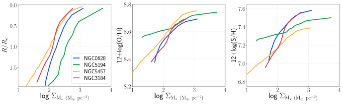
Figure 10.— Stellar mass surface density trends for the four CHAOS galaxies relative to galactocentric-radius (left panel), oxygen abundance (middle panel), and sulfur abundance (right panel). While NGC 5194 has abnormally flat abundance trends, the oxygen abundance of the three non-interacting galaxies closely correlates with stellar mass surface density.

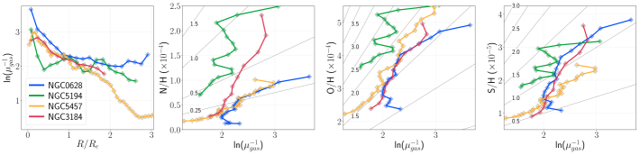
Figure 11.— Trends of the logarithm of the inverse of the gas fraction for the CHAOS sample. The radially-averaged profiles are similar for all four galaxies (first panel), whereas abundance trends for N/H (second panel), O/H (third panel), and S/H (last panel) show more significant variations. For the abundance versus inverse gas fraction trends, lines of constant elemental effective yield are drawn, where the yield labels are in that same units as the y-axis ($\times 10^{-4}$, $\times 10^{-4}$, and $\times 10^{-5}$ for N/H, O/H, and S/H, respectively).

5.2. Surface Density Relationships

A fundamental relationship of global galaxy evolution is the luminosity-metallicity relationship, which includes spiral disk galaxies (e.g., Garnett & Shields, 1987; Vila-Costas & Edmunds, 1993; Zaritsky et al., 1994). This relationship typically refers to the total or average metallicity of a galaxy, but what does this mean for the abundance gradients in individual spiral galaxies? While several recent studies support a characteristic oxygen abundance gradient for the main disk of spiral galaxies (e.g., Sánchez et al., 2014; Sánchez-Menguiano et al., 2018), Belfiore et al. (2017) reported an increasing oxygen abundance slope (dex/$R_{e}$) with stellar mass for SDSS-IV MaNGA (Bundy et al., 2015) galaxies with M${}_{\star}<10^{10.5}$ M_⊙. However, in a study of 49 local star-forming galaxies, Ho et al. (2015) found that metallicity gradients expressed in terms of the isophotal radius ($R_{25}$) did not correlate with either stellar mass or luminosity, but rather increase with decreasing total stellar mass when expressed in terms of dex/kpc (see, also, Pilyugin et al., 2019). Alternatively, Pilyugin et al. (2019) concluded in their study of MaNGA galaxies that oxygen abundance is governed by a galaxy’s rotational velocity. Despite these works, no clear evidence has emerged to conclusively determine the dependence of abundance gradients on basic galaxy properties or halo properties (e.g., rotational velocity).

Locally, the oxygen abundance trends of spiral galaxies have also been observed to correlate with stellar mass surface density (e.g., McCall, 1982; Edmunds & Pagel, 1984; Ryder, 1995; Garnett et al., 1997). In Figure 10, we examine the stellar mass surface density profiles for the CHAOS galaxies (see Appendix C for details). The left panel shows the typical trend of decreasing stellar mass surface density as you move further out in the disk, but with NGC 5194 having a slightly elevated density of stars compared to the others. In the middle and right panels, we plot the local surface mass-metallicity relationship for O/H and S/H, respectively. Similar to the global relationship (see, e.g., Tremonti et al., 2004), local metallicity measurements also increase with mass surface density and plateau at high mass values. This local trend is especially tight for the three non-interacting CHAOS galaxies.

The metallicity-surface density relationships in Figure 10 may reflect fundamental similarities in the evolution of non-barred, non-interacting spiral galaxies. For example, Ryder (1995) argues for a galaxy evolution model that includes self-regulating star formation, where energy injected into the ISM by newly-formed stars inhibits further star formation. These models were able to successfully reproduce the observed correlations between surface brightness and SFR (Dopita & Ryder, 1994) and surface mass density (e.g., Phillipps & Edmunds, 1991; Ryder, 1995; Garnett et al., 1997). The current work supports these ideas that stellar mass, gas mass, and SFR surface density are fundamental and interdependent parameters that govern the chemical evolution of spiral galaxies. A more thorough investigation of the dependence of metallicity on local properties with be conducted in the future with the entire CHAOS sample.

5.3. Effective Yields

In a simple closed-box model, assuming instantaneous recycling of stellar nucleosynthetic products and no gas flows, chemical evolution is solely a function of the gas fraction, $\mu_{\rm gas}$: $Z=y\cdot{\rm ln}(\mu^{-1})$, where $Z$ is the metallicity and $y$ is the metal yield. Inverting this equation, one can measure the effective yield, $y_{\rm eff}$, given the observed metallicity, $Z_{\rm obs}$, and gas fraction:

$$y_{\rm eff}=\frac{Z_{\rm obs}}{{\rm ln}(\mu_{\rm gas}^{-1})}.$$ (5)

In Figure 11, we plot the radially-averaged inverse gas fraction trends for the CHAOS sample (see Appendix C for the sources of the gas distributions). While the inverse gas fractions steadily decrease with increasing radius for all four galaxies (left panel), plotting abundance versus inverse gas fractions reveals different effective yield trends (three right panels). Nonetheless, the trends appear to be the most ordered for O/H and S/H, with similar slopes amongst the three non-interacting galaxies. The less ordered trends for N/H may then be revealing the effects of varying gas flows in each galaxy and the time effects of production in lower mass stars. Further, this picture is consistent with the result from theoretical models based on stochastically forced diffusion that most scatter in observed abundance gradients ($\sim 0.1$ dex) is due to stellar feedback and gas velocity dispersion (Krumholz & Ting, 2018).

Following Equation 5, these plots of abundance versus the inverse gas fraction trace the effective yield of the relevant element. The true yield is a function of stellar nucleosynthesis, but the effective yield (slope of $Z$-ln($\mu_{gas}^{-1}$) plots) will be altered from this value by gas inflows and outflows. In this context, the similar slopes in O/H and S/H versus ln($\mu_{gas}^{-1}$) are indicative of a closed-box effective yield of both oxygen and sulfur, whereas the O/H and S/H trends of NGC 5194 diverge as expected for gas flows associated with interacting galaxies. According to Figure 11, the CHAOS galaxies generally follow slopes of $0.5-1.25\times 10^{-5}$ for sulfur and $1.5-2.0\times 10^{-4}$ for oxygen, which corresponds to $y_{\rm eff}$(O)$=0.006-0.008$ assuming Z $=0.02$ Z_⊙ and 12+log(O/H)${}_{\odot}=8.69$ (Asplund et al., 2009). These $y_{\rm eff}$(O) values are consistent with the range of effective oxygen yields measured for spiral galaxies by Garnett (2002), spanning 0.0033–0.017. We note that the effective yield values Garnett (2002) found for NGC 628 and NGC 5194 are higher than our own, but this difference is largely accounted for by the offset in the measured abundance scales for these two galaxies.

6. Abundance Trends With Metallicity

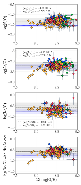
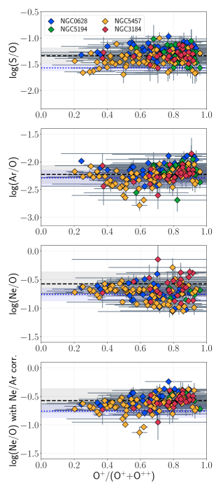
Figure 12.— Alpha-element ratios for the CHAOS sample versus oxygen abundances (left) and ionization fraction (right). In each panel, the solar value and uncertainty from Asplund et al. (2009) is labeled and plotted as a blue dotted-line and blue shaded-band, respectively. The weighted-average and uncertainty of the CHAOS data is also given and denoted by a black dashed-line and black shaded-band, respectively. The top two rows show the S/O and Ar/O ratios, both with relatively flat distributions. The Ar/O abundances for NGC 5457 were corrected by C16 using the Ar⁺⁺/S⁺⁺ relation shown in Figure 6, however, NGC 3184 uses the ICF(Ar) from Thuan et al. (1995). The bottom two rows show the Ne/O ratio using the standard Ne⁺⁺/O⁺⁺ ICF (third row) and further corrected for offsets in the Ne/Ar ratio (bottom row).

6.1. Alpha/O Abundances

Next, we turn our focus from abundance gradients to relative abundance trends with O/H metallicity. In Figure 12 we plot the relative abundances of $\alpha$-elements. In descending panel order we plot S/O, Ar/O, and Ne/O as a function of O/H (left side), where diamond points are color coded according to galaxy.

Stellar nucleosynthetic yields (e.g., Woosley & Weaver, 1995) indicate that $\alpha$-elements are predominantly produced on relatively short timescales by core-collapse supernovae (SNe; massive stars) explosions. The $\alpha$-element ratios in Figure 12 are, therefore, expected to be constant and so we plot the variance-weighted mean $\alpha$/O ratios of the CHAOS observations as black dashed lines in each panel. The average values are denoted in the upper left corners and can be compared to the solar values from Asplund et al. (2009, blue dotted line). The average CHAOS $\alpha$/O values are generally greater than solar, but individual galaxies also show slight shifts from one another.

Relative to the constant relationship assumed in each panel of Figure 12, the CHAOS observations visually show significant scatter and may also deviate in a systematic way. C16 discovered a significant population of low-ionization (high O⁺/O) H II regions in NGC 5457 with low Ne/O values. A deeper exploration of the $\alpha$/O ratios in that work revealed a lack of previous observations in the low-ionization regime and challenges in finding an appropriate ICF to use.

Similar to C16, in Section 3.2.5 we found a large dispersion in the Ne⁺⁺/O⁺⁺ ratios of the CHAOS galaxies for low-ionization H II regions. Additionally, many of these regions also exhibit exceptionally low values of log(Ar/Ne) (see Figure 6). This motivated us to apply a correction to the Ne/O abundances based on the offset in Ne/Ar from the average CHAOS value for low-ionization H II regions (O⁺/O $>0.5$). The updated Ne/O values, plotted in the bottom panel of Figure 12, show a smaller dispersion around the mean sample value, but with a few significant NGC 5457 outliers. While the proposed correction removes the bifurcation in Ne/O at low-ionization, it seems to over-correct Ne/O abundance for the nebulae with discordantly low Ar/O abundances.

Following C16, we further examine the $\alpha$/O dependence on ionization by plotting our $\alpha$/O ratios for the four CHAOS galaxies versus O⁺/O in the right column of Figure 12. For both Ar and S, there seems to be a small residual systematic dependence on ionization that is not adequately corrected for by C16 or other traditional ICFs. In this case, the high-ionization H II regions (O⁺/O $<0.5$) have S/O and Ar/O ratios that are generally under- and over-predicted, respectively, relative to the average, while the low-ionization H II regions (O⁺/O $>0.5$) seem to be evenly dispersed about the mean. In general, no simple corrections to the ICFs are yet apparent. Instead, we will derive new ICFs for the CHAOS data using updated photoionization models in a future paper.

6.2. N/O versus Metallicity

Historically, N/O enrichment has been studied as a function of total oxygen abundance owing to the relative ease of integrated-light galaxy observations. In this context, the observed scaling of nitrogen with oxygen has long been understood as a combination of primary nitrogen plus a linearly increasing fraction of secondary nitrogen that comes to dominate the total N/O relationship at intermediate metallicities (e.g., Vila-Costas & Edmunds, 1993; van Zee & Haynes, 2006; Berg et al., 2012). Note that the scatter of the N/O–O/H relationship reported in previous studies is often significantly larger than that of the CHAOS N/O radial gradients (e.g., van Zee & Haynes, 2006; Berg et al., 2012).

In Figure 13 we plot the N/O versus O/H values (left panel) and the N/O versus S/H value (right panel) for the CHAOS galaxies. For comparison, we also plot the empirical stellar N/O–O/H relationship from Nicholls et al. (2017) and measured abundances for nearby metal-poor dwarf galaxies from Berg et al. (2019), which should compose a primary N plateau at low O/H and S/H values. Despite the tight N/O radial gradients observed for individual CHAOS galaxies (see Figure 9), large dispersion is seen in N/O when plotted versus O/H, similar to previous N/O–O/H studies. Guided by the stellar relationship (purple line), our data do follow the general trend of low N/O due to primary nitrogen at low oxygen abundances, followed by increasing N/O, presumably as secondary nitrogen becomes prominent, at larger O/H (12+log(O/H)$\gtrsim$8.2). A similar trend is seen for N/O–S/H. Yet, individual galaxies in our sample clearly occupy different regions on the N/O versus O/H and N/O versus S/H plots. Interestingly, the collective trend of the four galaxies appears to produce a stronger correlation between N/O with S/H than O/H. However, significant scatter in seen for each galaxy, and the dispersions for the N/O–S/H and N/O–O/H relationships are consistent for each galaxy.

7. Understanding The
Universal N/O Gradient

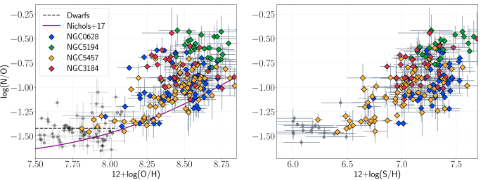
Figure 13.— N/O versus O/H (left) and S/H (right) for the CHAOS galaxies (diamonds) and local dwarf galaxies (grey circles). At low O/H or S/H, N is dominated by primary production and N/O is low (grey dashed line is the average primary N/O plateau of dwarfs). At larger O/H or S/H, secondary N production begins to increase N/O. This is demonstrated by the empirical trend of stellar abundances (purple line), however, individual H II regions show a large dispersion.

We now return to the universal N/O slope we found for the inner disks of CHAOS galaxies in Section 4.3. To understand the source of this trend, we must first understand how O and N are produced in these galaxies. Despite the ease at which both O and N emission are observed, discovering the origin of N is far more complex than O. Oxygen is primarily synthesized on short timescales by core-collapse SNe explosions of massive stars ($M\gtrsim 9M_{\odot}$, e.g., Heger et al., 2003). Nitrogen, on the other hand, is produced mainly by the CN branch of the CNO cycle, which can occur in the H-burning layer of both massive stars and intermediate mass stars ($1M_{\odot}<M<9M_{\odot}$). The slowest step of the CNO cycle is the conversion of ¹⁴N to ¹⁵O, which results in a pile up of ¹⁴N that can then be dredged-up by a convective layer. In metal-poor gas, the seed O and C needed for the CNO cycle may come from a He-burning phase. This path to N production is independent of the initial metal content of the star, and so is referred to as “primary” nucleosynthesis. In more enriched gas at higher metallicities the CNO cycle increases N production proportional to the initial metal composition (O and C) of the star. This type of N production is “secondary” nitrogen owing to its dependence on the metallicity of the star in which it was synthesized.

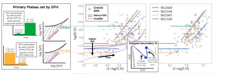
Figure 14.— Schematic of how a galaxy’s star formation history affects its overall N/O-O/H relationship. Right: average N/O versus O/H and S/H trends for the CHAOS sample. Secondary N slopes relative to S/H are similar for all four galaxies, however, the trends are offset from one another both vertically and horizontally. Left: two simple star formation histories and their resulting N/O-O/H trends are shown. On top, a star formation history with low star formation efficiency at early times allows N/O to build up, raising the primary plateau and shifting the transition to secondary dominance to the right. On the bottom, a star formation history with high star formation rate at early times produces significant oxygen ahead of nitrogen production, setting a lower primary N/O plateau and O/H transition to secondary N. In addition to these differences, the lower-right inset plot shows that the N/O ratios of individual H II regions are sensitive to time since the onset of the most recent burst, driving scatter from the average relationships.

7.1. Offsets Between Individual Galaxies

A schematic of nitrogen production for the CHAOS galaxies is shown in Figure 14. The radial gradient fits to the N/O, O/H, and S/H relationships are combined to produce the plotted N/O versus O/H relationship (middle panel) and N/O versus S/H (right panel) for each galaxy. The progressively increasing N/O values at smaller galactocentric distance correspond to increasing O/H abundance, as is expected for secondary N production. This results in parallel secondary N/O slopes for the N/O–S/H trends in Figure 14, and similar slopes in the N/O–O/H relationship for the three non-interacting galaxies. However, the individual relationships are distinct in two ways. First, each galaxy has a different primary plateau level, indicating large variations in their star formation histories, and, second, a different O/H transition value for when secondary N becomes important and turns the N/O curve upwards.

Henry et al. (2000) found that chemical evolution models differing only by their assumed star formation efficiencies (SFEs) produced a range of primary N/O plateaus. We illustrate the effect of varying the SFE by over-plotting the Henry et al. (2000) constant SFR models, where efficiency has been varied by a factor of 25, on our N/O versus O/H data in Figure 14. For low SFRs, the build-up of oxygen is slow and on the order of the lag time before intermediate-mass stars begin ejecting nitrogen. This allows a high N/O plateau to be established at low oxygen abundances (darkest purple curve). On the other hand, high star formation rates early in the star formation history (SFH) form a large number of massive stars that produce greater levels of oxygen ahead of N enrichment, establishing a lower plateau (lightest purple curve) and shifting the entire N/O–O/H trend in Figure 14 to the right towards greater O/H. In between these scenarios, continuous star formation with roughly 250 Myr between bursts will result in N and O increasing in lockstep, dependent on the elemental yields. The coupling of the N/O plateau with galaxy SFH is also reported by cosmological hydrodynamical simulations of individual regions within spatially-resolved galaxies (Vincenzo & Kobayashi, 2018). In these simulations, asymptotic giant branch (AGB) stars contribute significant N at low O/H, but the exact value of the primary N/O plateau will vary from galaxy to galaxy according to the relative contributions from SNe and AGB stars, as determined by their galaxy formation time and SFH.

On the left-hand side of Figure 14, we extend the highest N/O plateau from NGC 5194 (green) and the lowest N/O plateau from NGC 5457 (yellow). Based on the above discussion, for the low N/O plateau of NGC 5457, we can put forth a star formation history scenario in which the star formation efficiency was high early in the galaxy’s evolution, allowing oxygen to build up from many bursts of star formation before nitrogen was returned from longer-lived intermediate mass stars. Due to the higher level of nucleosynthetic products from massive stars, contributions from secondary nitrogen production may dominate over primary nitrogen production at relatively low O/H and S/H values. On the other hand, the high N/O plateau of NGC 5194 could be due to a star formation history in which low star formation efficiency at early times allows nitrogen production, although delayed, to keep pace with oxygen and sulfur production and enrich the ISM. Here we assume low star formation efficiency to mean either constant, low star formation rates or long quiescent periods between bursts. In this scenario, primary nitrogen production is the dominant mechanism until the galaxy reaches relatively high O/H. Note, however, that this is a very simplistic model where N/O is changing monotonically; in a hierarchical galaxy building scenario that may not be true.

In summary, the primary N/O plateau sensitively probes the SFH of a galaxy, rather than being set by the ratio of N to O yields, and explains the large range of plateau levels observed for spiral galaxies. When this offset is accounted for, the N/O plateau then informs the primary N production yields and the universal N/O gradient (see Figure 13) is a direct probe of the secondary N yields of intermediate mass stars.

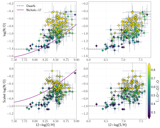
Figure 15.— Top: N/O relationships for the CHAOS sample relative to O/H (left) and S/H (right). Bottom: scaled N/O trends relative to O/H (left) and S/H (right), where the differences in the star formation histories of individual galaxies are removed by vertically shifting their primary N/O plateaus to align with log(N/O) $=-1.0$. For reference, the empirical stellar N/O–O/H trend from Nicholls et al. (2017) and metal-poor N/O plateau for local dwarfs (Berg et al., 2019) are also plotted. All plots are color-coded by the O⁺/O ratio, or low-ionization fraction, and show a persistent trend of increasing N/O with O⁺/O regardless of the N/O normalization.

7.2. The Scatter in the
N/O–O/H Relationship

In Figure 13 we plotted the N/O–O/H trend of the CHAOS galaxies and found large observed scatter in N/O for a given O/H. Given the tight correlations measured for the CHAOS N/O radial gradients (see Table 2), this scatter seems to be real. Previous works have suggested that some of this scatter may be due to the time-dependent nature of N/O production (i.e., a N/O “clock”; Garnett, 1990; Pilyugin, 1999; Henry et al., 2006). A directly observable effect of an aging ionizing stellar population is an increasing fraction of low- to high-ionization gas in the H II region (see, for example, how the shape of the ionizing continuum changes with age in Chisholm et al., 2019).

In Figure 15 we reproduce the N/O–O/H and N/O–S/H trends, color-coded by the O⁺/O ratio, or low-ionization fraction. Interestingly, the overall trend of increasing N/O seems to be ordered by ionization or age. In the bottom panels of Figure 15, we scale N/O (as was done in Section 4.3) by shifting the vertical offsets in order to remove differences in individual primary N/O plateaus and SFHs, yet the overall trend of increasing N/O ordered by ionization remains. Nearly all of the CHAOS points now have N/O abundances that are lower relative to the scaled average stellar relationship of Nicholls et al. (2017), suggesting that the physics of a recent burst of star formation has the effect of shifting the N/O abundances downward, as expected for a recent injection of newly synthesized oxygen. The regions with the lowest N/O also have high ionization. However, the standard N/O clock assumes regions with high N/O ratios have experienced a burst of star formation followed by a long quiescent period that allowed their gas to be enriched with N from slow-evolving stars after a few 100 Myrs. Given the fact that typical H II regions are younger than $\sim 10$ Myr, the simple delayed-release N clock hypothesis fails to explain our observed spread in N/O at a given O/H.

Alternatively, Coziol et al. (1999) suggested high N/O ratios in starburst nucleus galaxies could result if N production occurs from a different, older population of intermediate-mass stars, such as would result from a sequence of bursts of star formation. Similarly, Berg et al. (2019) used chemical evolution models of dwarf galaxies to show that N/O was elevated in regions experiencing an extended duration of star formation (continuous star formation) up to 0.4 Gyr. Then, the overall effect of observing a large sample of H II regions with a range of luminosity-weighted average stellar population ages may be to produce the vertical spread in N/O at a given O/H seen in Figure 15.

Perhaps another reason for the increased scatter of the N/O–O/H trends relative to the N/O–$R_{g}$ relationships is the possibility that N production is (or behaves as) a secondary function of the carbon abundance, rather than the typically assumed oxygen abundance (Henry et al., 2000). Recently, Groh et al. (2019) investigated grids of stellar models at very low metallicities and found that the ratio between nitrogen and carbon abundances (N/C) remains generally unchanged for non-rotating stellar models during their main sequence phase. However, the N/C production can increase by as much as 10–20$\times$ in rotating models at the end of the main sequence. Thus, variations in stellar rotation speeds of different burst populations could result in significant effects on setting the low-metallicity stage. Additionally, Berg et al. (2019) showed differential outflows of interstellar medium gas can affect the primary C/O and N/O ratios. Since O and S are produced on different timescales than N, newly synthesized O and S may be preferentially lost in SNe winds and these outflows may have a greater probability of escape in the outer parts of the disk.

At higher metallicities, where the effects of stellar winds become more important, other authors have suggested that Wolf-Rayet stars can expel significant amounts of N resulting in local regions of N/O enrichment. For the CHAOS sample, however, we do not find any correlation in the N/O dispersion with the Wolf-Rayet features sometimes seen in the optical spectra.

Another hypothesis is that the dispersion in N/O could be explained if we are consistently underestimating the O/H abundance in low-ionization nebula. We have tested this hypothesis by looking at the offset in O/H abundance from the radial gradients relative to the secondary N/O radial gradient offsets and find some evidence of an anti-correlation, but it cannot explain all of the dispersion observed in N/O.

In summary, while we have observed a universal N/O gradient for the CHAOS galaxies that seems to be tied to the nucleosynthetic yields of N, we also observe a large dispersion when plotted relative to O/H. We have discussed several possible scenarios that could contribute to the N/O–O/H scatter, including extended star formation periods, differential outflows, and a secondary dependence on carbon abundance, but the importance of these contributions has not yet been determined. At this time, the source of the scatter in the N/O–O/H relationship remains an open question, but with several promising possibilities for future study.

Table 2Linear Fits to CHAOS Gradients

$y$	$x$	Galaxy	$\#$ Reg.	Equation	$\sigma_{\rm{int.}}$	$\sigma_{\rm{tot.}}$
12+log(O/H) (dex)	$R_{g}$ ($R_{25}^{-1}$)	NGC 0628	45	$y=(8.71\pm 0.06)-(0.40\pm 0.11)\times x$	0.12	0.13
		NGC 5194	28	$y=(8.75\pm 0.09)-(0.27\pm 0.15)\times x$	0.07	0.10
		NGC 5457	72	$y=(8.78\pm 0.04)-(0.90\pm 0.07)\times x$	0.10	0.11
		NGC 3184	30	$y=(8.74\pm 0.16)-(0.48\pm 0.28)\times x$	0.14	0.16
	$R_{g}$ ($R_{e}^{-1}$)	NGC 0628	45	$y=(8.70\pm 0.06)-(0.11\pm 0.03)\times x$	0.12	0.13
		NGC 5194	28	$y=(8.67\pm 0.08)-(0.07\pm 0.04)\times x$	0.07	0.10
		NGC 5457	72	$y=(8.75\pm 0.03)-(0.20\pm 0.02)\times x$	0.10	0.11
		NGC 3184	30	$y=(8.71\pm 0.15)-(0.18\pm 0.10)\times x$	0.14	0.16
12+log(S/H) (dex)	$R_{g}$ ($R_{e}^{-1}$)	NGC 0628	45	$y=(7.60\pm 0.06)-(0.19\pm 0.03)\times x$	0.12	0.13
		NGC 5194	28	$y=(7.51\pm 0.11)-(0.10\pm 0.05)\times x$	0.07	0.12
		NGC 5457	72	$y=(7.40\pm 0.05)-(0.23\pm 0.03)\times x$	0.18	0.19
		NGC 3184	30	$y=(7.59\pm 0.15)-(0.34\pm 0.11)\times x$	0.11	0.13
log(N/O) (dex)	$R_{g}$ ($R_{25}^{-1}$)	NGC 0628	59	$y=(-0.64\pm 0.04)-(0.61\pm 0.06)\times x$	0.10	0.11
		NGC 5194	28	$y=(-0.34\pm 0.09)-(0.44\pm 0.16)\times x$	0.05	0.08
		NGC 5457	72	$y=(-0.73\pm 0.03)-(0.81\pm 0.06)\times x$	0.07	0.10
		NGC 3184	30	$y=(-0.30\pm 0.13)-(0.83\pm 0.22)\times x$	0.04	0.08
	$R_{g}$ ($R_{e}^{-1}$)	NGC 0628	59	$y=(-0.65\pm 0.03)-(0.18\pm 0.02)\times x$	0.10	0.11
		NGC 5194	28	$y=(-0.34\pm 0.09)-(0.12\pm 0.04)\times x$	0.05	0.08
		NGC 5457	72	$y=(-0.74\pm 0.03)-(0.18\pm 0.01)\times x$	0.08	0.10
		NGC 3184	30	$y=(-0.30\pm 0.12)-(0.35\pm 0.09)\times x$	0.05	0.08
log(N/O)prim. (dex)		NGC 0628	11	$y=-1.28$		0.13
		NGC 5194	4	$y=-0.71$		0.03
		NGC 5457	15	$y=-1.38$		0.13
		NGC 3184	0	$y=-$1.15		$\cdots$
log(N/O)sec. (dex)	$R_{g}$ ($R_{e}^{-1}$)	NGC 0628	38	$y=(-0.43\pm 0.05)-(0.34\pm 0.04)\times x$	0.06	0.07
		NGC 5194	20	$y=(-0.27\pm 0.18)-(0.17\pm 0.11)\times x$	0.07	0.09
		NGC 5457	45	$y=(-0.58\pm 0.07)-(0.30\pm 0.05)\times x$	0.06	0.08
		NGC 3184	30	$y=(-0.30\pm 0.12)-(0.35\pm 0.09)\times x$	0.05	0.08
Scaled
log(N/O)sec. (dex)	$R_{g}$ ($R_{e}^{-1}$)	All Four	133	$y=(-0.15\pm 0.03)-(0.36\pm 0.02)\times x$	0.05	0.09
		Non-Inter.	113	$y=(-0.16\pm 0.03)-(0.34\pm 0.02)\times x$	0.05	0.08

Note. — Linear fits to trends in abundance versus radius for the four CHAOS galaxies. The fits are determined using the Bayesian linear mixture model implemented in the linmix python code, which fits data with uncertainties on two variables, including explicit treatment of intrinsic scatter. The $y$ and $x$ variables are given in the first two columns, with the number of associated H II regions used in the fit listed in Column 4. The resulting best fit is given in Column 5, with uncertainties on both the slope and $y-$intercept. Columns 6 and 7 list the intrinsic and total uncertainties, $\sigma_{tot.}$ and $\sigma_{int.}$. Note that the primary log(N/O) value given for NGC 3184 is italicized to indicate that this quantity is an estimated value from the extrapolated secondary fit, and not a measurement.

8. CONCLUSIONS

This work is the fourth paper in a series presenting the on-going results of the CHemical Abundances of Spirals survey (CHAOS Berg et al., 2015), a project that is building a large database of direct abundance measurements spanning a large range in physical conditions in H II regions across the disks of nearby spiral galaxies. Previous results for NGCC 628, NGC 5194, and NGC 5457 have been reported individually in papers i–iii. Here we present new LBT/MODS spectra of 52 H II regions in NGC 3184 to amass a high-quality, coherent sample of 175 direct-abundances from the first four CHAOS galaxies.

Taking advantage of the direct $T_{e}$ measurements from one or more auroral line detections in 190 individual H II regions, we confirm our previous results that $T_{e}$[S III] and $T_{e}$[N II] provide robust measures of electron temperature in the metal-rich H II regions typical of spiral galaxies. Specifically, the $T_{e}$[S III]–$T_{e}$[N II] trend, which characterizes the intermediate- to low-ionization zone temperatures, is especially tight for low-ionization H II regions (low $F_{\lambda 5007}/F_{\lambda 3727}$) with temperatures of $T_{e}\lesssim 8\times 10^{3}$ K. Unsurprisingly, we also find that the $T_{e}$[O III]–$T_{e}$[S III] relationship is tightly correlated for high-ionization H II regions (high $F_{\lambda 5007}/F_{\lambda 3727}$). Given the observed dichotomy in temperature dispersions with ionization of the nebulae, we recommend new ionization-based temperature priorities and apply them to abundance determinations for the four CHAOS galaxies.

Prioritizing temperatures derived from [O III], [S III] or [N II] depending on the average ionization of the observed nebula, we measure the relative and absolute abundance trends of O, N, S, Ar, and Ne for the CHAOS sample. While the average $\alpha$/O abundances of the CHAOS sample are consistent within the uncertainties of flat trends, we find evidence of systematic offsets that further depend on ionization and will likely require more sophisticated ionization correction factors to correct. For O/H, we examine gradients normalized to both the isophotal radius ($R_{25}$) and the effective radius ($R_{e}$). In contrast to some recent empirical abundance studies, we do not find a universal direct-O/H gradient when radius is plotted relative $R_{e}$, but rather measure unique slopes ranging from $-0.07$ to $-0.20$ dex/$R_{e}$.

Similarly, we examine the N/O gradient of our sample using both $R_{25}$ and $R_{e}$. While each galaxy in our sample has a unique zero point offset, interpreted here as different primary N/O plateaus set by differences in their star formation histories, the secondary N/O slopes all appear to be the same. We, therefore, determine the first measurement of a universal N/O gradient of $\alpha_{\rm N/O}=-0.33$ dex/$R_{e}$ for $R_{g}/R_{e}<2.0$, where N is dominated by secondary production, and which can be used to constrain stellar yields.

As expected for two alpha elements, we find similar gradients for S/H and O/H for the CHAOS galaxies. These trends suggest S/H can serve as a useful direct abundance diagnostic in the absence of O/H, such as data sets lacking the blue wavelength coverage of [O III] $\lambda$4363. However, direct S/H abundances will generally be significantly more uncertain than direct O/H abundances owing to the often large sulfur ICF uncertainties. Given that the observable ionic states of S probe lower ionization and excitation energies than O, S/H might be more appropriate for characterizing abundances in the moderate- to metal-rich H II regions of spiral galaxies. Further work is needed to better constrain S ICFs and quantify their uncertainties in order to improve S/H abundance determinations.

Appendix A CHAOS iv: NGC 3184 Measurements

In Tables 3–A we present details for the CHAOS optical MODS/LBT spectroscopic observations of NGC 3184 used in this work, the measured emission line intensities, and the calculated ionic and total abundances.

Table 3NGC 3184 MODS/LBT Observations

H ii	R.A.	Dec.	Rg	R/R25	Rg	Offset	Auroral Line Detections					Wolf
Region	(2000)	(2000)	(arcsec)		(kpc)	(arcsec)	[O iii]	[N ii]	[S iii]	[O ii]	[S ii]	Rayet
Total Detections:							5	20	16	36	42	6
NGC3184+2.7-0.5	10:18:17.0	41:25:26.52	2.10	0.009	0.12	+2.7,-0.5		✓		✓
NGC3184+24.4-11.6	10:18:19.0	41:25:15.42	27.11	0.122	1.54	+24.4,-11.6
NGC3184+27.0-10.7	10:18:19.2	41:25:16.27	29.29	0.132	1.66	+27.0,-10.7
NGC3184-2.7-47.5	10:18:16.6	41:24:39.55	47.18	0.213	2.68	-2.7,-47.5					✓
NGC3184-6.4-48.7	10:18:16.2	41:24:38.34	48.81	0.220	2.77	-6.4,-48.7
NGC3184-11.3-50.1	10:18:15.8	41:24:36.94	51.22	0.231	2.91	-11.3,-50.1				✓	✓
NGC3184-1.1+60.6	10:18:16.7	41:26:27.58	61.02	0.275	3.46	-1.1,+60.6					✓
NGC3184-19.4-62.1	10:18:15.1	41:24:24.89	65.15	0.293	3.70	-19.4,-62.1					✓
NGC3184-59.5-37.7	10:18:11.5	41:24:49.33	72.86	0.328	4.13	-59.5,-37.7		✓		✓	✓	✓
NGC3184-70.7-27.1	10:18:10.5	41:24:59.91	78.94	0.356	4.48	-70.7,-27.1
NGC3184-70.7-27.1	10:18:10.5	41:24:59.91	78.94	0.356	4.48	-70.7,-27.1
NGC3184+51.2+60.4	10:18:21.4	41:26:27.44	80.47	0.362	4.56	+51.2,+60.4		✓		✓	✓
NGC3184+78.4+34.5	10:18:23.8	41:26:01.51	88.11	0.397	5.00	+78.4,+34.5
NGC3184-15.0-88.4	10:18:15.5	41:23:58.57	89.56	0.403	5.08	-15.0,-88.4			✓
NGC3184-14.9-95.5	10:18:15.5	41:23:51.54	96.45	0.434	5.47	-14.9,-95.5		✓		✓	✓
NGC3184+62.1-75.3	10:18:22.3	41:24:11.72	98.37	0.443	5.58	+62.1,-75.3					✓
NGC3184-71.1+67.7	10:18:10.5	41:26:34.64	100.99	0.455	5.73	-71.1,+67.7			✓	✓	✓
NGC3184-82.5+57.7	10:18:09.5	41:26:24.66	104.12	0.469	5.91	-82.5,+57.7		✓		✓	✓
NGC3184-90.9-43.7	10:18:08.7	41:24:43.30	104.69	0.472	5.94	-90.9,-43.7					✓
NGC3184+62.1-86.8	10:18:22.3	41:24:00.14	107.41	0.484	6.09	+62.1,-86.8					✓
NGC3184-94.2+43.8	10:18:08.4	41:26:10.74	108.04	0.487	6.13	-94.2+43.8				✓	✓
NGC3184+48.9+97.3	10:18:21.1	41:27:04.27	109.86	0.495	6.23	+48.9+97.3		✓	✓	✓	✓
NGC3184+107.7-15.4	10:18:26.4	41:25:11.53	112.32	0.506	6.37	+107.7,-15.4			✓	✓	✓
NGC3184-67.3+87.1	10:18:10.8	41:26:54.10	112.44	0.506	6.38	-67.3,+87.1		✓	✓	✓	✓	✓
NGC3184-96.3+58.2	10:18:08.2	41:26:25.15	116.55	0.525	6.61	-96.3,+58.2					✓
NGC3184+19.6-115.5	10:18:18.5	41:23:31.55	116.69	0.526	6.62	+19.6,-115.5		✓		✓	✓
NGC3184+18.8-115.7	10:18:18.5	41:23:31.27	116.82	0.526	6.63	+18.8,-115.7		✓		✓	✓
NGC3184+18.8-115.7	10:18:18.5	41:23:31.27	116.82	0.526	6.63	+18.8,-115.7		✓		✓	✓
NGC3184+75.7+89.1	10:18:23.5	41:26:56.14	118.91	0.536	6.74	+75.7,+89.1		✓	✓	✓	✓	✓
NGC3184-72.8+91.3	10:18:10.3	41:26:58.26	119.27	0.537	6.77	-72.8,+91.3	✓	✓	✓	✓	✓	✓
NGC3184-114.2+11.4	10:18:06.6	41:25:38.38	120.11	0.541	6.81	-114.2,+11.4					✓
NGC3184+16.4+119.8	10:18:18.3	41:27:26.77	121.30	0.546	6.88	+16.4,+119.8		✓	✓	✓	✓
NGC3184+116.2-33.6	10:18:27.1	41:24:53.32	124.67	0.562	7.07	+116.2,-33.6				✓	✓
NGC3184-106.3+57.0	10:18:07.3	41:26:24.02	125.21	0.564	7.10	-106.3,+57.0				✓	✓
NGC3184+110.6-52.0	10:18:26.6	41:24:34.99	125.42	0.565	7.11	+110.6,-52.0			✓	✓	✓
NGC3184-64.+105.8	10:18:11.1	41:27:12.74	125.68	0.566	7.13	-64.1,+105.8				✓	✓
NGC3184-96.7+74.3	10:18:08.2	41:26:41.26	125.74	0.566	7.13	-96.7,+74.3		✓		✓	✓
NGC3184+8.2-132.1	10:18:17.5	41:23:14.87	131.95	0.594	7.48	+8.2,-132.1		✓		✓	✓
NGC3184+94.9-91.5	10:18:25.2	41:23:55.46	133.75	0.602	7.59	+94.9,-91.5			✓	✓		✓
NGC3184+100.6+84.2	10:18:25.7	41:26:51.22	134.12	0.604	7.61	+100.6,+84.2		✓		✓	✓
NGC3184+14.9-139.6	10:18:18.1	41:23:07.40	139.95	0.630	7.94	+14.9,-139.6	✓		✓	✓	✓	✓
NGC3184+63.8+126.0	10:18:22.5	41:27:32.95	142.48	0.642	8.08	+63.8,+126.0			✓	✓	✓
NGC3184+123.8+76.5	10:18:27.8	41:26:43.47	149.52	0.674	8.48	+123.8,+76.5			✓	✓	✓
NGC3184+70.7+132.5	10:18:23.1	41:27:39.49	151.65	0.683	8.60	+70.7,+132.5				✓	✓
NGC3184-145.8+8.7	10:18:03.8	41:25:35.64	152.62	0.687	8.66	-145.8,+8.7
NGC3184+41.9+148.8	10:18:20.5	41:27:55.80	155.31	0.700	8.81	+41.9,+148.8		✓	✓	✓	✓
NGC3184+80.0-148.2	10:18:23.9	41:22:58.76	169.18	0.762	9.60	+80.0,-148.2	✓		✓	✓	✓
NGC3184-117.5-120.0	10:18:06.4	41:23:26.93	171.67	0.773	9.74	-117.5,-120.0				✓	✓
NGC3184-110.6-127.6	10:18:07.0	41:23:19.41	172.10	0.775	9.76	-110.6,-127.6		✓		✓	✓
NGC3184-93.3-142.3	10:18:08.5	41:23:04.68	172.45	0.777	9.78	-93.3,-142.3	✓			✓	✓
NGC3184-169.8-22.2	10:18:01.7	41:25:04.72	178.74	0.805	10.14	-169.8,-22.2		✓		✓	✓
NGC3184-172.5-30.2	10:18:01.5	41:24:56.73	182.69	0.823	10.36	-172.5,-30.2	✓	✓	✓	✓	✓

Note. — Observing logs for Hii regions observed in NGC 3184 using MODS on the LBT on the UT dates of March 24, 2012 and January 6, 2013. Each field was observed over an integrated exposure time of 1200s on clear nights, with, on average $\sim$1$\farcs$00 seeing, and airmasses less than 1.3. Slit ID, composed of the galaxy name and the offset in R.A. and Dec., in arcseconds, from the central position listed in Table 1 is listed in Column 1. The right ascension and declination of the individual Hii regions are given in units of hours, minutes, and seconds, and degrees, arcminutes, and arcseconds respectively in columns 2 and 3. The de-projected distances of Hii regions from the center of the galaxy in arcseconds, fraction of R₂₅, and in kpc are listed in the Columns 4-6. Columns 7-11 highlight which regions have [O iii] $\lambda$4363, [N ii] $\lambda$5755, [S iii] $\lambda$6312, [O ii] $\lambda\lambda 7320,7330$ and [S ii] $\lambda\lambda$4068,4076 auroral lines detections at the 3$\sigma$ significance level. Finally, column 12 indicates which Hii regions have Wolf-Rayet feature detections.

Table 4Emission-Line Intensities and Equivalent Widths for LBT Observations of H II regions in NGC 3184

	$I(\lambda)/I(\mbox{H}\beta)$
Ion	+2.7-0.5	+24.4-11.6	+27.0-10.7	-2.7-47.5	-6.4-48.7	-11.3-50.1	-1.1+60.6
H14 $\lambda$3721	0.015$\pm$0.001	0.018$\pm$0.004	0.024$\pm$0.002	0.016$\pm$0.002	0.019$\pm$0.001	0.021$\pm$0.001	0.009$\pm$0.001
[O ii] $\lambda$3727	0.374$\pm$0.007	0.844$\pm$0.019	0.839$\pm$0.014	0.745$\pm$0.137	0.672$\pm$0.014	0.678$\pm$0.011	0.566$\pm$0.010
H13 $\lambda$3734	0.018$\pm$0.001	0.022$\pm$0.004	0.029$\pm$0.003	0.020$\pm$0.003	0.024$\pm$0.002	0.026$\pm$0.001	0.011$\pm$0.001
H12 $\lambda$3750	0.003$\pm$0.005	0.021$\pm$0.004	0.030$\pm$0.008	0.050$\pm$0.007	0.024$\pm$0.005	0.043$\pm$0.002	0.005$\pm$0.002
H11 $\lambda$3770	0.053$\pm$0.004	0.040$\pm$0.007	0.076$\pm$0.006	0.050$\pm$0.005	0.031$\pm$0.002	0.048$\pm$0.001	$\cdots$
H10 $\lambda$3797	0.039$\pm$0.003	0.048$\pm$0.010	0.062$\pm$0.006	0.043$\pm$0.006	0.051$\pm$0.003	0.056$\pm$0.003	0.025$\pm$0.002
He I $\lambda$3819	0.012$\pm$0.002	0.036$\pm$0.007	0.017$\pm$0.006	0.040$\pm$0.007	0.005$\pm$0.002	0.010$\pm$0.001	$\cdots$
H9 $\lambda$3835	0.073$\pm$0.001	0.085$\pm$0.002	0.099$\pm$0.006	0.057$\pm$0.011	0.071$\pm$0.005	0.073$\pm$0.002	0.026$\pm$0.003
[Ne iii] $\lambda$3868	0.024$\pm$0.003	0.011$\pm$0.005	$\cdots$	0.044$\pm$0.008	0.008$\pm$0.002	0.003$\pm$0.002	0.011$\pm$0.002
He I $\lambda$3888	0.090$\pm$0.004	0.032$\pm$0.004	0.013$\pm$0.006	0.046$\pm$0.015	0.025$\pm$0.003	0.037$\pm$0.002	0.033$\pm$0.002
H8 $\lambda$3889	0.076$\pm$0.005	0.089$\pm$0.018	0.118$\pm$0.011	0.081$\pm$0.012	0.098$\pm$0.006	0.108$\pm$0.006	0.049$\pm$0.003
He I $\lambda$3964	0.004$\pm$0.005	0.009$\pm$0.006	$\cdots$	0.013$\pm$0.012	0.002$\pm$0.004	0.003$\pm$0.002	$\cdots$
[Ne iii] $\lambda$3967	0.072$\pm$0.005	0.030$\pm$0.005	0.007$\pm$0.005	0.056$\pm$0.013	$\cdots$	0.025$\pm$0.002	0.031$\pm$0.004
H7 $\lambda$3970	0.114$\pm$0.007	0.129$\pm$0.026	0.173$\pm$0.017	0.119$\pm$0.018	0.144$\pm$0.009	0.161$\pm$0.009	0.074$\pm$0.005
[Ne iii] $\lambda$4011	$\cdots$	0.007$\pm$0.006	$\cdots$	0.007$\pm$0.004	0.002$\pm$0.002	0.005$\pm$0.003	0.003$\pm$0.001
He I $\lambda$4026	0.005$\pm$0.002	$\cdots$	$\cdots$	0.034$\pm$0.003	0.012$\pm$0.002	0.014$\pm$0.001	$\cdots$
[S ii] $\lambda$4068	0.003$\pm$0.003	0.005$\pm$0.002	$\cdots$	0.023$\pm$0.005	0.008$\pm$0.003	0.012$\pm$0.002	0.014$\pm$0.002
[S ii] $\lambda$4076	0.005$\pm$0.005	0.007$\pm$0.003	$\cdots$	0.017$\pm$0.001	0.010$\pm$0.001	0.016$\pm$0.003	0.010$\pm$0.002
H$\delta$ $\lambda$4101	0.314$\pm$0.006	0.234$\pm$0.007	0.214$\pm$0.006	0.241$\pm$0.007	0.238$\pm$0.007	0.289$\pm$0.004	0.188$\pm$0.007
He I $\lambda$4120	0.018$\pm$0.005	$\cdots$	0.007$\pm$0.004	0.009$\pm$0.003	0.001$\pm$0.001	0.002$\pm$0.001	$\cdots$
He I $\lambda$4143	0.001$\pm$0.003	$\cdots$	$\cdots$	0.005$\pm$0.004	$\cdots$	0.006$\pm$0.001	$\cdots$
H$\gamma$ $\lambda$4340	0.476$\pm$0.007	0.452$\pm$0.012	0.434$\pm$0.011	0.437$\pm$0.011	0.436$\pm$0.013	0.483$\pm$0.007	0.409$\pm$0.009
[O iii] $\lambda$4363	$\cdots$	$\cdots$	$\cdots$	0.010$\pm$0.004	0.006$\pm$0.004	$\cdots$	0.003$\pm$0.003
He I $\lambda$4387	$\cdots$	0.004$\pm$0.001	0.004$\pm$0.004	$\cdots$	0.003$\pm$0.001	0.004$\pm$0.001	$\cdots$
He I $\lambda$4471	0.014$\pm$0.002	0.004$\pm$0.003	0.021$\pm$0.004	0.032$\pm$0.002	0.018$\pm$0.002	0.016$\pm$0.001	0.001$\pm$0.001
[Fe iii] $\lambda$4658	0.008$\pm$0.001	0.023$\pm$0.003	$\cdots$	$\cdots$	0.001$\pm$0.001	$\cdots$	0.009$\pm$0.001
He II $\lambda$4686	0.011$\pm$0.001	0.014$\pm$0.001	0.006$\pm$0.004	0.006$\pm$0.003	0.003$\pm$0.001	$\cdots$	0.003$\pm$0.001
H$\beta$ $\lambda$4861	1.000$\pm$0.006	1.000$\pm$0.021	1.000$\pm$0.018	1.000$\pm$0.020	1.000$\pm$0.014	1.000$\pm$0.008	1.000$\pm$0.012
He I $\lambda$4921	0.009$\pm$0.002	0.015$\pm$0.012	0.018$\pm$0.010	0.004$\pm$0.011	$\cdots$	0.007$\pm$0.004	0.001$\pm$0.004
[O iii] $\lambda$4959	0.050$\pm$0.002	0.033$\pm$0.012	0.027$\pm$0.011	0.031$\pm$0.012	0.008$\pm$0.007	0.016$\pm$0.004	0.025$\pm$0.004
[O iii] $\lambda$5007	0.133$\pm$0.002	0.075$\pm$0.013	0.050$\pm$0.010	0.121$\pm$0.011	0.034$\pm$0.006	0.054$\pm$0.004	0.058$\pm$0.004
He I $\lambda$5015	0.009$\pm$0.002	0.003$\pm$0.011	0.014$\pm$0.009	0.014$\pm$0.011	0.011$\pm$0.006	0.008$\pm$0.004	0.004$\pm$0.004
[N ii] $\lambda$5755	0.002$\pm$0.001	0.004$\pm$0.008	0.008$\pm$0.007	$\cdots$	$\cdots$	0.007$\pm$0.003	0.001$\pm$0.002
He I $\lambda$5876	0.068$\pm$0.001	0.132$\pm$0.009	0.080$\pm$0.007	0.071$\pm$0.007	0.047$\pm$0.004	0.075$\pm$0.003	0.036$\pm$0.002
[O ı] $\lambda$6300	0.030$\pm$0.001	0.032$\pm$0.007	0.017$\pm$0.005	0.010$\pm$0.005	0.019$\pm$0.003	0.023$\pm$0.003	0.006$\pm$0.002
[S iii] $\lambda$6312	0.002$\pm$0.001	$\cdots$	0.011$\pm$0.005	$\cdots$	$\cdots$	0.003$\pm$0.002	0.002$\pm$0.002
[O ı] $\lambda$6363	0.002$\pm$0.001	$\cdots$	0.022$\pm$0.005	0.006$\pm$0.005	0.009$\pm$0.003	0.008$\pm$0.002	$\cdots$
[N ii] $\lambda$6548	0.272$\pm$0.012	0.409$\pm$0.017	0.350$\pm$0.009	0.368$\pm$0.011	0.303$\pm$0.008	0.320$\pm$0.007	0.269$\pm$0.006
H$\alpha$ $\lambda$6563	3.123$\pm$0.070	3.020$\pm$0.092	2.950$\pm$0.065	2.929$\pm$0.091	2.993$\pm$0.079	3.179$\pm$0.049	2.795$\pm$0.070
[N ii] $\lambda$6584	0.850$\pm$0.020	1.245$\pm$0.039	1.119$\pm$0.026	1.164$\pm$0.035	0.951$\pm$0.026	1.000$\pm$0.016	0.847$\pm$0.020
He I $\lambda$6678	0.016$\pm$0.001	0.023$\pm$0.001	0.018$\pm$0.002	0.021$\pm$0.001	0.020$\pm$0.001	0.018$\pm$0.001	0.012$\pm$0.001
[S ii] $\lambda$6717	0.302$\pm$0.008	0.301$\pm$0.009	0.295$\pm$0.007	0.283$\pm$0.010	0.352$\pm$0.010	0.359$\pm$0.007	0.317$\pm$0.008
[S ii] $\lambda$6731	0.262$\pm$0.006	0.220$\pm$0.007	0.218$\pm$0.005	0.207$\pm$0.007	0.247$\pm$0.007	0.257$\pm$0.004	0.228$\pm$0.005
He I $\lambda$7065	0.009$\pm$0.001	0.009$\pm$0.003	0.006$\pm$0.004	0.012$\pm$0.004	0.002$\pm$0.001	0.006$\pm$0.002	0.006$\pm$0.002
[Ar iii] $\lambda$7135	0.010$\pm$0.001	0.019$\pm$0.002	0.019$\pm$0.004	0.027$\pm$0.004	0.004$\pm$0.001	0.011$\pm$0.002	0.010$\pm$0.002
[O ii] $\lambda$7320	0.004$\pm$0.001	0.015$\pm$0.010	0.002$\pm$0.004	0.010$\pm$0.005	0.005$\pm$0.001	0.004$\pm$0.002	0.006$\pm$0.002
[O ii] $\lambda$7330	$\cdots$	0.015$\pm$0.010	0.014$\pm$0.004	0.002$\pm$0.004	0.001$\pm$0.001	0.009$\pm$0.002	0.003$\pm$0.002
[Ar iii] $\lambda$7751	0.011$\pm$0.001	0.013$\pm$0.003	0.003$\pm$0.001	0.004$\pm$0.002	0.008$\pm$0.002	$\cdots$	0.005$\pm$0.003
P13 $\lambda$8665	$\cdots$	0.001$\pm$0.005	0.011$\pm$0.013	0.012$\pm$0.015	0.006$\pm$0.007	$\cdots$	0.012$\pm$0.009
P12 $\lambda$8750	0.019$\pm$0.005	0.051$\pm$0.008	0.025$\pm$0.018	0.023$\pm$0.021	0.013$\pm$0.008	2.520$\pm$0.022	0.027$\pm$0.012
P11 $\lambda$8862	0.025$\pm$0.005	$\cdots$	0.001$\pm$0.015	0.025$\pm$0.019	0.011$\pm$0.008	$\cdots$	0.015$\pm$0.010
P10 $\lambda$9015	0.044$\pm$0.002	0.014$\pm$0.004	0.017$\pm$0.004	0.019$\pm$0.006	0.018$\pm$0.003	0.017$\pm$0.003	0.020$\pm$0.003
[S iii] $\lambda$9069	0.097$\pm$0.002	0.111$\pm$0.005	0.089$\pm$0.004	0.155$\pm$0.006	0.088$\pm$0.004	0.118$\pm$0.004	0.079$\pm$0.003
P9 $\lambda$9229	0.028$\pm$0.002	0.014$\pm$0.004	0.022$\pm$0.004	0.027$\pm$0.005	0.019$\pm$0.004	0.023$\pm$0.003	0.022$\pm$0.003
[S iii] $\lambda$9532	0.261$\pm$0.004	0.247$\pm$0.009	0.259$\pm$0.008	0.431$\pm$0.012	0.223$\pm$0.007	0.316$\pm$0.008	0.206$\pm$0.005
P8 $\lambda$9546	0.020$\pm$0.003	0.076$\pm$0.008	0.037$\pm$0.008	0.081$\pm$0.011	0.076$\pm$0.007	0.099$\pm$0.007	0.041$\pm$0.006
$E(B-V)$	0.161$\pm$0.013	0.698$\pm$0.020	0.594$\pm$0.016	0.522$\pm$0.020	0.463$\pm$0.018	0.238$\pm$0.010	0.205$\pm$0.019
FHβ	119.73$\pm$0.40	39.25$\pm$0.55	44.83$\pm$0.62	32.25$\pm$0.42	43.70$\pm$0.41	47.51$\pm$0.20	31.11$\pm$0.31
Ion	-19.4-62.1	-59.5-37.7	-70.7-27.1	-70.7-27.1	+51.2+60.4	+78.4+34.5	-15.0-88.4
H14 $\lambda$3721	0.013$\pm$0.001	0.016$\pm$0.001	0.018$\pm$0.001	0.021$\pm$0.001	0.017$\pm$0.001	0.019$\pm$0.001	0.014$\pm$0.014
[O ii] $\lambda$3727	0.769$\pm$0.015	0.765$\pm$0.013	0.672$\pm$0.011	0.700$\pm$0.009	0.764$\pm$0.008	1.019$\pm$0.013	0.997$\pm$0.712
H13 $\lambda$3734	0.016$\pm$0.001	0.019$\pm$0.001	0.022$\pm$0.002	0.027$\pm$0.002	0.021$\pm$0.001	0.023$\pm$0.001	0.018$\pm$0.018
H12 $\lambda$3750	0.016$\pm$0.004	0.019$\pm$0.001	0.022$\pm$0.006	0.051$\pm$0.005	0.021$\pm$0.001	0.008$\pm$0.003	0.010$\pm$0.010
H11 $\lambda$3770	0.028$\pm$0.003	0.033$\pm$0.002	0.051$\pm$0.001	0.076$\pm$0.007	0.031$\pm$0.002	0.034$\pm$0.003	0.037$\pm$0.037
H10 $\lambda$3797	0.034$\pm$0.002	0.042$\pm$0.003	0.048$\pm$0.004	0.058$\pm$0.004	0.045$\pm$0.002	0.051$\pm$0.002	0.038$\pm$0.038
He I $\lambda$3819	0.008$\pm$0.003	$\cdots$	$\cdots$	$\cdots$	0.001$\pm$0.002	0.011$\pm$0.002	$\cdots$
H9 $\lambda$3835	0.045$\pm$0.002	0.056$\pm$0.001	0.072$\pm$0.005	0.094$\pm$0.004	0.061$\pm$0.001	0.059$\pm$0.003	0.062$\pm$0.062
[Ne iii] $\lambda$3868	0.006$\pm$0.002	0.004$\pm$0.001	$\cdots$	$\cdots$	0.004$\pm$0.002	0.023$\pm$0.002	0.004$\pm$0.004
He I $\lambda$3888	0.036$\pm$0.003	0.064$\pm$0.003	0.049$\pm$0.003	0.054$\pm$0.005	0.043$\pm$0.002	0.026$\pm$0.005	0.061$\pm$0.061
H8 $\lambda$3889	0.066$\pm$0.004	0.082$\pm$0.006	0.094$\pm$0.007	0.114$\pm$0.007	0.086$\pm$0.004	0.099$\pm$0.004	0.073$\pm$0.073
He I $\lambda$3964	0.001$\pm$0.003	$\cdots$	$\cdots$	$\cdots$	$\cdots$	$\cdots$	0.001$\pm$0.001
[Ne iii] $\lambda$3967	0.018$\pm$0.004	0.034$\pm$0.004	$\cdots$	$\cdots$	0.030$\pm$0.002	$\cdots$	0.040$\pm$0.040
H7 $\lambda$3970	0.099$\pm$0.006	0.122$\pm$0.009	0.140$\pm$0.011	0.170$\pm$0.011	0.128$\pm$0.006	0.148$\pm$0.006	0.108$\pm$0.108
[Ne iii] $\lambda$4011	0.014$\pm$0.002	0.002$\pm$0.001	$\cdots$	$\cdots$	$\cdots$	0.004$\pm$0.003	$\cdots$
He I $\lambda$4026	$\cdots$	$\cdots$	$\cdots$	$\cdots$	$\cdots$	$\cdots$	0.002$\pm$0.002
[S ii] $\lambda$4068	0.017$\pm$0.002	0.003$\pm$0.003	$\cdots$	0.001$\pm$0.002	0.014$\pm$0.002	0.004$\pm$0.002	0.008$\pm$0.008
[S ii] $\lambda$4076	0.003$\pm$0.002	0.003$\pm$0.003	$\cdots$	$\cdots$	0.003$\pm$0.003	$\cdots$	0.007$\pm$0.007
H$\delta$ $\lambda$4101	0.198$\pm$0.007	0.282$\pm$0.005	0.230$\pm$0.005	0.250$\pm$0.006	0.256$\pm$0.004	0.245$\pm$0.006	0.289$\pm$0.289
He I $\lambda$4120	0.004$\pm$0.002	0.003$\pm$0.002	$\cdots$	$\cdots$	$\cdots$	$\cdots$	0.009$\pm$0.009
He I $\lambda$4143	$\cdots$	$\cdots$	$\cdots$	$\cdots$	$\cdots$	$\cdots$	$\cdots$
H$\gamma$ $\lambda$4340	0.397$\pm$0.013	0.462$\pm$0.007	0.396$\pm$0.010	0.410$\pm$0.008	0.471$\pm$0.006	0.480$\pm$0.008	0.462$\pm$0.462
[O iii] $\lambda$4363	$\cdots$	$\cdots$	$\cdots$	$\cdots$	0.003$\pm$0.002	0.007$\pm$0.004	$\cdots$
He I $\lambda$4387	$\cdots$	$\cdots$	$\cdots$	$\cdots$	0.001$\pm$0.001	$\cdots$	$\cdots$
He I $\lambda$4471	$\cdots$	0.009$\pm$0.001	0.017$\pm$0.004	0.016$\pm$0.004	0.015$\pm$0.001	0.005$\pm$0.003	0.006$\pm$0.006
[Fe iii] $\lambda$4658	0.007$\pm$0.002	0.013$\pm$0.002	0.017$\pm$0.003	0.013$\pm$0.002	0.003$\pm$0.001	0.004$\pm$0.001	0.026$\pm$0.026
He II $\lambda$4686	0.013$\pm$0.002	0.009$\pm$0.001	0.023$\pm$0.004	0.020$\pm$0.003	0.002$\pm$0.001	0.001$\pm$0.001	0.023$\pm$0.023
H$\beta$ $\lambda$4861	1.000$\pm$0.017	1.000$\pm$0.006	1.000$\pm$0.012	1.000$\pm$0.013	1.000$\pm$0.009	1.000$\pm$0.016	1.000$\pm$1.000
He I $\lambda$4921	0.006$\pm$0.009	0.004$\pm$0.001	$\cdots$	$\cdots$	$\cdots$	$\cdots$	0.006$\pm$0.006
[O iii] $\lambda$4959	0.033$\pm$0.009	0.031$\pm$0.001	0.030$\pm$0.006	0.027$\pm$0.006	0.029$\pm$0.005	0.015$\pm$0.009	0.043$\pm$0.043
[O iii] $\lambda$5007	0.097$\pm$0.009	0.089$\pm$0.001	0.080$\pm$0.006	0.065$\pm$0.007	0.086$\pm$0.005	0.076$\pm$0.009	0.116$\pm$0.116
He I $\lambda$5015	0.003$\pm$0.008	0.012$\pm$0.001	0.005$\pm$0.005	0.003$\pm$0.006	0.008$\pm$0.005	0.012$\pm$0.009	0.006$\pm$0.006
[N ii] $\lambda$5755	0.006$\pm$0.005	0.003$\pm$0.001	0.004$\pm$0.004	0.003$\pm$0.005	0.004$\pm$0.001	0.006$\pm$0.002	0.004$\pm$0.004
He I $\lambda$5876	0.052$\pm$0.006	0.076$\pm$0.001	0.032$\pm$0.005	0.034$\pm$0.005	0.065$\pm$0.003	0.066$\pm$0.006	0.068$\pm$0.068
[O ı] $\lambda$6300	0.003$\pm$0.004	0.012$\pm$0.001	$\cdots$	$\cdots$	0.025$\pm$0.003	0.026$\pm$0.005	0.024$\pm$0.024
[S iii] $\lambda$6312	$\cdots$	0.002$\pm$0.001	0.004$\pm$0.004	0.004$\pm$0.004	0.004$\pm$0.003	$\cdots$	0.003$\pm$0.003
[O ı] $\lambda$6363	0.006$\pm$0.004	0.004$\pm$0.001	$\cdots$	$\cdots$	0.008$\pm$0.003	0.009$\pm$0.005	0.010$\pm$0.010
[N ii] $\lambda$6548	0.239$\pm$0.006	0.311$\pm$0.005	0.251$\pm$0.009	0.262$\pm$0.009	0.306$\pm$0.011	0.337$\pm$0.009	0.308$\pm$0.308
H$\alpha$ $\lambda$6563	2.783$\pm$0.073	3.036$\pm$0.045	2.804$\pm$0.051	2.833$\pm$0.057	3.056$\pm$0.034	3.147$\pm$0.088	2.894$\pm$2.894
[N ii] $\lambda$6584	0.759$\pm$0.018	0.950$\pm$0.012	0.782$\pm$0.014	0.809$\pm$0.016	0.944$\pm$0.011	1.083$\pm$0.030	0.954$\pm$0.954
He I $\lambda$6678	0.012$\pm$0.001	0.020$\pm$0.001	0.006$\pm$0.001	0.008$\pm$0.001	0.018$\pm$0.001	0.022$\pm$0.001	0.021$\pm$0.021
[S ii] $\lambda$6717	0.282$\pm$0.007	0.299$\pm$0.004	0.299$\pm$0.006	0.293$\pm$0.006	0.286$\pm$0.003	0.360$\pm$0.009	0.337$\pm$0.337
[S ii] $\lambda$6731	0.193$\pm$0.005	0.220$\pm$0.003	0.204$\pm$0.005	0.200$\pm$0.004	0.208$\pm$0.003	0.252$\pm$0.007	0.243$\pm$0.243
He I $\lambda$7065	0.008$\pm$0.004	0.011$\pm$0.001	0.002$\pm$0.001	0.003$\pm$0.002	0.008$\pm$0.002	0.009$\pm$0.005	0.009$\pm$0.009
[Ar iii] $\lambda$7135	0.013$\pm$0.003	0.018$\pm$0.001	$\cdots$	$\cdots$	0.019$\pm$0.002	0.027$\pm$0.005	0.021$\pm$0.021
[O ii] $\lambda$7320	0.002$\pm$0.004	0.003$\pm$0.001	0.001$\pm$0.001	0.002$\pm$0.002	0.010$\pm$0.002	0.005$\pm$0.006	0.006$\pm$0.006
[O ii] $\lambda$7330	0.002$\pm$0.004	0.004$\pm$0.001	0.002$\pm$0.001	0.001$\pm$0.002	0.008$\pm$0.002	0.008$\pm$0.006	0.005$\pm$0.005
[Ar iii] $\lambda$7751	0.003$\pm$0.002	0.008$\pm$0.001	0.004$\pm$0.002	0.006$\pm$0.003	0.006$\pm$0.002	0.006$\pm$0.004	0.008$\pm$0.008
P13 $\lambda$8665	0.005$\pm$0.014	0.010$\pm$0.002	0.003$\pm$0.006	0.004$\pm$0.009	0.010$\pm$0.008	0.011$\pm$0.020	0.011$\pm$0.011
P12 $\lambda$8750	0.040$\pm$0.019	0.013$\pm$0.003	0.008$\pm$0.009	$\cdots$	0.015$\pm$0.010	$\cdots$	0.009$\pm$0.009
P11 $\lambda$8862	0.015$\pm$0.016	0.013$\pm$0.003	$\cdots$	0.008$\pm$0.010	0.023$\pm$0.009	0.019$\pm$0.023	0.013$\pm$0.013
P10 $\lambda$9015	0.019$\pm$0.005	0.020$\pm$0.001	0.019$\pm$0.004	0.020$\pm$0.006	0.021$\pm$0.003	0.021$\pm$0.007	0.022$\pm$0.022
[S iii] $\lambda$9069	0.083$\pm$0.006	0.168$\pm$0.001	0.051$\pm$0.004	0.058$\pm$0.006	0.138$\pm$0.003	0.184$\pm$0.008	0.177$\pm$0.177
P9 $\lambda$9229	0.017$\pm$0.006	0.027$\pm$0.001	0.023$\pm$0.004	0.025$\pm$0.006	0.023$\pm$0.003	0.029$\pm$0.008	0.030$\pm$0.030
[S iii] $\lambda$9532	0.195$\pm$0.010	0.484$\pm$0.003	0.184$\pm$0.008	0.197$\pm$0.011	0.391$\pm$0.007	0.503$\pm$0.016	0.506$\pm$0.506
P8 $\lambda$9546	0.011$\pm$0.011	0.036$\pm$0.002	0.031$\pm$0.008	0.028$\pm$0.012	0.055$\pm$0.006	0.031$\pm$0.016	0.014$\pm$0.014
$E(B-V)$	0.315$\pm$0.020	0.243$\pm$0.011	0.254$\pm$0.013	0.157$\pm$0.014	0.387$\pm$0.008	0.165$\pm$0.016	$\cdots$
FHβ	20.84$\pm$0.28	225.85$\pm$0.79	37.34$\pm$0.28	15.63$\pm$0.13	54.00$\pm$0.34	14.23$\pm$0.15	77.63$\pm$nan
Ion	-14.9-95.5	+62.1-75.3	-71.1+67.7	-82.5+57.7	-90.9-43.7	+62.1-86.8	-94.2+43.8
H14 $\lambda$3721	0.018$\pm$0.002	0.024$\pm$0.002	0.015$\pm$0.001	0.010$\pm$0.001	0.021$\pm$0.002	0.019$\pm$0.001	0.021$\pm$0.001
[O ii] $\lambda$3727	1.256$\pm$0.033	1.285$\pm$0.021	1.278$\pm$0.016	1.610$\pm$0.024	1.786$\pm$0.041	1.071$\pm$0.020	1.762$\pm$0.024
H13 $\lambda$3734	0.023$\pm$0.003	0.029$\pm$0.003	0.018$\pm$0.001	0.013$\pm$0.001	0.026$\pm$0.003	0.023$\pm$0.001	0.026$\pm$0.002
H12 $\lambda$3750	0.025$\pm$0.005	0.058$\pm$0.004	0.019$\pm$0.001	0.006$\pm$0.002	0.029$\pm$0.003	0.034$\pm$0.001	0.044$\pm$0.003
H11 $\lambda$3770	0.082$\pm$0.007	0.086$\pm$0.005	0.029$\pm$0.001	0.032$\pm$0.002	0.057$\pm$0.005	0.040$\pm$0.002	0.040$\pm$0.003
H10 $\lambda$3797	0.049$\pm$0.007	0.064$\pm$0.006	0.040$\pm$0.002	0.028$\pm$0.002	0.056$\pm$0.006	0.050$\pm$0.002	0.056$\pm$0.004
He I $\lambda$3819	0.011$\pm$0.006	$\cdots$	$\cdots$	$\cdots$	0.001$\pm$0.005	0.008$\pm$0.001	$\cdots$
H9 $\lambda$3835	0.096$\pm$0.006	0.097$\pm$0.004	0.049$\pm$0.001	0.044$\pm$0.002	0.084$\pm$0.003	0.078$\pm$0.002	0.072$\pm$0.003
[Ne iii] $\lambda$3868	0.027$\pm$0.004	0.029$\pm$0.004	0.012$\pm$0.001	0.022$\pm$0.002	0.038$\pm$0.005	0.007$\pm$0.002	0.023$\pm$0.005
He I $\lambda$3888	0.064$\pm$0.008	0.053$\pm$0.003	0.059$\pm$0.002	0.080$\pm$0.002	0.044$\pm$0.006	0.058$\pm$0.004	0.036$\pm$0.002
H8 $\lambda$3889	0.096$\pm$0.013	0.123$\pm$0.011	0.077$\pm$0.003	0.055$\pm$0.003	0.108$\pm$0.011	0.098$\pm$0.004	0.107$\pm$0.007
He I $\lambda$3964	0.027$\pm$0.005	$\cdots$	0.003$\pm$0.002	0.001$\pm$0.003	0.014$\pm$0.005	0.005$\pm$0.003	0.006$\pm$0.002
[Ne iii] $\lambda$3967	$\cdots$	$\cdots$	0.023$\pm$0.002	0.049$\pm$0.003	$\cdots$	$\cdots$	$\cdots$
H7 $\lambda$3970	0.142$\pm$0.019	0.183$\pm$0.016	0.115$\pm$0.005	0.081$\pm$0.004	0.159$\pm$0.017	0.145$\pm$0.005	0.156$\pm$0.010
[Ne iii] $\lambda$4011	$\cdots$	$\cdots$	$\cdots$	$\cdots$	0.028$\pm$0.003	0.002$\pm$0.001	$\cdots$
He I $\lambda$4026	$\cdots$	$\cdots$	0.001$\pm$0.001	$\cdots$	0.001$\pm$0.003	0.011$\pm$0.001	0.013$\pm$0.002
[S ii] $\lambda$4068	0.017$\pm$0.002	0.015$\pm$0.004	0.011$\pm$0.001	0.018$\pm$0.001	0.015$\pm$0.004	0.011$\pm$0.002	0.020$\pm$0.002
[S ii] $\lambda$4076	0.016$\pm$0.002	0.021$\pm$0.003	0.007$\pm$0.001	0.009$\pm$0.001	0.013$\pm$0.002	0.004$\pm$0.001	0.012$\pm$0.003
H$\delta$ $\lambda$4101	0.260$\pm$0.007	0.258$\pm$0.004	0.235$\pm$0.004	0.193$\pm$0.006	0.240$\pm$0.007	0.235$\pm$0.005	0.208$\pm$0.005
He I $\lambda$4120	$\cdots$	0.004$\pm$0.002	$\cdots$	$\cdots$	$\cdots$	0.006$\pm$0.001	$\cdots$
He I $\lambda$4143	$\cdots$	$\cdots$	$\cdots$	$\cdots$	$\cdots$	$\cdots$	$\cdots$
H$\gamma$ $\lambda$4340	0.459$\pm$0.012	0.451$\pm$0.009	0.440$\pm$0.006	0.426$\pm$0.008	0.414$\pm$0.014	0.427$\pm$0.009	0.434$\pm$0.008
[O iii] $\lambda$4363	0.003$\pm$0.002	$\cdots$	0.003$\pm$0.002	0.004$\pm$0.003	0.005$\pm$0.003	$\cdots$	0.009$\pm$0.003
He I $\lambda$4387	$\cdots$	0.001$\pm$0.001	$\cdots$	$\cdots$	0.011$\pm$0.002	0.001$\pm$0.001	0.008$\pm$0.001
He I $\lambda$4471	0.009$\pm$0.002	0.014$\pm$0.002	0.024$\pm$0.001	0.015$\pm$0.001	0.041$\pm$0.002	0.022$\pm$0.001	0.022$\pm$0.002
[Fe iii] $\lambda$4658	0.008$\pm$0.001	0.006$\pm$0.001	0.007$\pm$0.001	0.005$\pm$0.001	0.003$\pm$0.003	0.001$\pm$0.001	$\cdots$
He II $\lambda$4686	0.014$\pm$0.001	0.008$\pm$0.001	0.005$\pm$0.001	0.007$\pm$0.001	0.005$\pm$0.002	0.012$\pm$0.001	0.004$\pm$0.001
H$\beta$ $\lambda$4861	1.000$\pm$0.009	1.000$\pm$0.011	1.000$\pm$0.007	1.000$\pm$0.012	1.000$\pm$0.021	1.000$\pm$0.010	1.000$\pm$0.014
He I $\lambda$4921	0.004$\pm$0.004	0.014$\pm$0.005	0.007$\pm$0.003	0.004$\pm$0.006	0.004$\pm$0.012	0.008$\pm$0.005	0.008$\pm$0.007
[O iii] $\lambda$4959	0.101$\pm$0.004	0.065$\pm$0.005	0.078$\pm$0.003	0.080$\pm$0.006	0.167$\pm$0.013	0.080$\pm$0.005	0.130$\pm$0.008
[O iii] $\lambda$5007	0.259$\pm$0.004	0.151$\pm$0.005	0.235$\pm$0.003	0.247$\pm$0.007	0.525$\pm$0.015	0.204$\pm$0.005	0.405$\pm$0.009
He I $\lambda$5015	0.008$\pm$0.003	0.013$\pm$0.005	0.013$\pm$0.003	0.010$\pm$0.006	0.022$\pm$0.012	0.016$\pm$0.005	0.009$\pm$0.007
[N ii] $\lambda$5755	0.003$\pm$0.001	0.007$\pm$0.003	0.004$\pm$0.002	0.006$\pm$0.001	$\cdots$	0.003$\pm$0.003	0.002$\pm$0.004
He I $\lambda$5876	0.068$\pm$0.003	0.053$\pm$0.004	0.087$\pm$0.002	0.077$\pm$0.004	0.389$\pm$0.012	0.087$\pm$0.004	0.072$\pm$0.004
[O ı] $\lambda$6300	0.010$\pm$0.002	0.018$\pm$0.003	0.016$\pm$0.001	0.040$\pm$0.003	0.024$\pm$0.008	0.007$\pm$0.003	0.029$\pm$0.003
[S iii] $\lambda$6312	0.006$\pm$0.002	0.004$\pm$0.003	0.004$\pm$0.001	0.005$\pm$0.003	0.020$\pm$0.008	0.006$\pm$0.003	0.003$\pm$0.003
[O ı] $\lambda$6363	0.003$\pm$0.002	0.003$\pm$0.003	0.005$\pm$0.001	0.011$\pm$0.003	0.017$\pm$0.007	$\cdots$	0.006$\pm$0.003
[N ii] $\lambda$6548	0.210$\pm$0.011	0.253$\pm$0.012	0.317$\pm$0.007	0.322$\pm$0.008	0.279$\pm$0.009	0.242$\pm$0.006	0.304$\pm$0.008
H$\alpha$ $\lambda$6563	3.008$\pm$0.045	2.848$\pm$0.190	2.841$\pm$0.046	2.809$\pm$0.054	2.818$\pm$0.064	2.866$\pm$0.043	2.799$\pm$0.046
[N ii] $\lambda$6584	0.636$\pm$0.011	0.760$\pm$0.012	0.982$\pm$0.017	1.003$\pm$0.019	0.855$\pm$0.019	0.747$\pm$0.012	0.961$\pm$0.017
He I $\lambda$6678	0.016$\pm$0.001	0.015$\pm$0.001	0.023$\pm$0.001	0.021$\pm$0.001	0.024$\pm$0.001	0.025$\pm$0.001	0.021$\pm$0.001
[S ii] $\lambda$6717	0.251$\pm$0.005	0.308$\pm$0.005	0.320$\pm$0.006	0.416$\pm$0.007	0.307$\pm$0.007	0.213$\pm$0.004	0.331$\pm$0.006
[S ii] $\lambda$6731	0.177$\pm$0.004	0.213$\pm$0.004	0.228$\pm$0.004	0.292$\pm$0.005	0.211$\pm$0.005	0.148$\pm$0.003	0.239$\pm$0.004
He I $\lambda$7065	0.005$\pm$0.001	0.007$\pm$0.002	0.010$\pm$0.001	0.011$\pm$0.003	$\cdots$	0.015$\pm$0.002	0.015$\pm$0.002
[Ar iii] $\lambda$7135	0.016$\pm$0.001	0.006$\pm$0.002	0.034$\pm$0.001	0.029$\pm$0.003	0.011$\pm$0.002	0.025$\pm$0.002	0.041$\pm$0.002
[O ii] $\lambda$7320	0.003$\pm$0.002	0.003$\pm$0.002	0.007$\pm$0.001	0.011$\pm$0.003	0.007$\pm$0.032	0.003$\pm$0.002	0.010$\pm$0.003
[O ii] $\lambda$7330	0.005$\pm$0.001	0.005$\pm$0.002	0.004$\pm$0.001	0.010$\pm$0.003	0.017$\pm$0.032	$\cdots$	0.009$\pm$0.002
[Ar iii] $\lambda$7751	0.009$\pm$0.002	0.008$\pm$0.003	0.009$\pm$0.001	0.010$\pm$0.003	0.010$\pm$0.004	0.009$\pm$0.003	0.013$\pm$0.003
P13 $\lambda$8665	0.004$\pm$0.006	0.018$\pm$0.010	0.008$\pm$0.004	0.006$\pm$0.011	0.007$\pm$0.013	0.013$\pm$0.009	0.004$\pm$0.008
P12 $\lambda$8750	0.017$\pm$0.009	0.010$\pm$0.011	0.007$\pm$0.006	0.029$\pm$0.016	$\cdots$	0.009$\pm$0.014	0.009$\pm$0.009
P11 $\lambda$8862	0.013$\pm$0.007	0.016$\pm$0.011	0.015$\pm$0.005	0.018$\pm$0.014	0.007$\pm$0.015	0.024$\pm$0.012	0.012$\pm$0.008
P10 $\lambda$9015	0.010$\pm$0.003	0.010$\pm$0.004	0.020$\pm$0.002	0.018$\pm$0.004	$\cdots$	0.022$\pm$0.004	0.017$\pm$0.003
[S iii] $\lambda$9069	0.100$\pm$0.003	0.082$\pm$0.004	0.192$\pm$0.002	0.171$\pm$0.004	$\cdots$	0.166$\pm$0.004	0.217$\pm$0.004
P9 $\lambda$9229	0.008$\pm$0.003	0.012$\pm$0.004	0.028$\pm$0.002	0.027$\pm$0.004	$\cdots$	0.021$\pm$0.004	0.025$\pm$0.003
[S iii] $\lambda$9532	0.253$\pm$0.005	0.189$\pm$0.008	0.499$\pm$0.004	0.411$\pm$0.009	0.201$\pm$0.010	0.434$\pm$0.008	0.558$\pm$0.008
P8 $\lambda$9546	0.030$\pm$0.005	0.043$\pm$0.008	0.034$\pm$0.003	0.061$\pm$0.009	$\cdots$	0.057$\pm$0.007	0.030$\pm$0.006
$E(B-V)$	0.270$\pm$0.012	0.253$\pm$0.016	0.276$\pm$0.010	0.268$\pm$0.015	0.377$\pm$0.017	0.272$\pm$0.011	0.569$\pm$0.012
FHβ	56.05$\pm$0.34	47.72$\pm$0.31	73.60$\pm$0.39	26.89$\pm$0.26	18.50$\pm$0.26	39.40$\pm$0.27	51.48$\pm$0.54
Ion	+48.9+97.3	+107.7-15.4	-67.3+87.1	-96.3+58.2	+19.6-115.5	+18.8-115.7	+18.8-115.7
H14 $\lambda$3721	0.017$\pm$0.002	0.022$\pm$0.001	0.016$\pm$0.001	0.019$\pm$0.001	0.018$\pm$0.001	0.019$\pm$0.001	0.018$\pm$0.001
[O ii] $\lambda$3727	1.787$\pm$0.018	1.501$\pm$0.017	1.506$\pm$0.016	2.028$\pm$0.029	1.488$\pm$0.009	1.527$\pm$0.008	1.485$\pm$0.009
H13 $\lambda$3734	0.021$\pm$0.002	0.027$\pm$0.001	0.020$\pm$0.001	0.023$\pm$0.001	0.022$\pm$0.001	0.023$\pm$0.001	0.023$\pm$0.001
H12 $\lambda$3750	0.026$\pm$0.003	0.044$\pm$0.002	0.025$\pm$0.001	0.041$\pm$0.004	0.034$\pm$0.002	0.035$\pm$0.002	0.031$\pm$0.002
H11 $\lambda$3770	0.030$\pm$0.002	0.032$\pm$0.002	0.034$\pm$0.002	0.048$\pm$0.003	0.040$\pm$0.003	0.040$\pm$0.003	0.035$\pm$0.002
H10 $\lambda$3797	0.045$\pm$0.004	0.059$\pm$0.002	0.044$\pm$0.002	0.051$\pm$0.003	0.048$\pm$0.003	0.051$\pm$0.002	0.049$\pm$0.003
He I $\lambda$3819	0.014$\pm$0.003	0.006$\pm$0.004	$\cdots$	0.004$\pm$0.003	0.010$\pm$0.002	0.008$\pm$0.002	0.005$\pm$0.002
H9 $\lambda$3835	0.069$\pm$0.003	0.082$\pm$0.002	0.063$\pm$0.001	0.078$\pm$0.003	0.073$\pm$0.003	0.074$\pm$0.003	0.069$\pm$0.003
[Ne iii] $\lambda$3868	0.022$\pm$0.002	0.017$\pm$0.001	0.012$\pm$0.001	0.016$\pm$0.003	0.013$\pm$0.001	0.014$\pm$0.001	0.014$\pm$0.001
He I $\lambda$3888	0.076$\pm$0.003	0.070$\pm$0.001	0.056$\pm$0.002	0.044$\pm$0.003	0.056$\pm$0.001	0.054$\pm$0.002	0.050$\pm$0.002
H8 $\lambda$3889	0.087$\pm$0.008	0.113$\pm$0.003	0.086$\pm$0.005	0.099$\pm$0.005	0.092$\pm$0.005	0.098$\pm$0.004	0.095$\pm$0.006
He I $\lambda$3964	0.018$\pm$0.002	$\cdots$	0.003$\pm$0.002	0.008$\pm$0.003	$\cdots$	0.007$\pm$0.001	0.008$\pm$0.002
[Ne iii] $\lambda$3967	0.040$\pm$0.003	$\cdots$	0.043$\pm$0.002	$\cdots$	0.009$\pm$0.001	0.003$\pm$0.001	$\cdots$
H7 $\lambda$3970	0.129$\pm$0.012	0.168$\pm$0.005	0.129$\pm$0.007	0.147$\pm$0.008	0.137$\pm$0.007	0.145$\pm$0.005	0.140$\pm$0.009
[Ne iii] $\lambda$4011	$\cdots$	0.004$\pm$0.001	$\cdots$	0.015$\pm$0.003	0.006$\pm$0.001	0.002$\pm$0.001	$\cdots$
He I $\lambda$4026	0.009$\pm$0.002	0.005$\pm$0.002	0.007$\pm$0.001	0.015$\pm$0.002	0.014$\pm$0.001	0.007$\pm$0.001	0.004$\pm$0.001
[S ii] $\lambda$4068	0.023$\pm$0.002	0.022$\pm$0.002	0.011$\pm$0.002	0.015$\pm$0.003	0.009$\pm$0.001	0.011$\pm$0.001	0.012$\pm$0.002
[S ii] $\lambda$4076	0.018$\pm$0.002	0.008$\pm$0.001	0.005$\pm$0.002	0.006$\pm$0.002	0.004$\pm$0.001	0.006$\pm$0.001	0.007$\pm$0.001
H$\delta$ $\lambda$4101	0.235$\pm$0.004	0.300$\pm$0.004	0.271$\pm$0.003	0.218$\pm$0.005	0.243$\pm$0.002	0.249$\pm$0.002	0.253$\pm$0.002
He I $\lambda$4120	0.014$\pm$0.001	0.004$\pm$0.002	0.003$\pm$0.001	0.002$\pm$0.003	$\cdots$	0.001$\pm$0.001	$\cdots$
He I $\lambda$4143	0.001$\pm$0.002	$\cdots$	$\cdots$	$\cdots$	$\cdots$	0.001$\pm$0.001	0.003$\pm$0.001
H$\gamma$ $\lambda$4340	0.444$\pm$0.009	0.495$\pm$0.006	0.452$\pm$0.005	0.428$\pm$0.009	0.452$\pm$0.004	0.463$\pm$0.003	0.475$\pm$0.004
[O iii] $\lambda$4363	0.002$\pm$0.002	$\cdots$	0.001$\pm$0.001	$\cdots$	0.001$\pm$0.001	0.001$\pm$0.001	0.004$\pm$0.001
He I $\lambda$4387	0.007$\pm$0.001	0.002$\pm$0.001	0.001$\pm$0.001	0.007$\pm$0.002	0.002$\pm$0.001	0.003$\pm$0.001	0.005$\pm$0.001
He I $\lambda$4471	0.026$\pm$0.001	0.017$\pm$0.002	0.021$\pm$0.001	0.020$\pm$0.001	0.021$\pm$0.001	0.018$\pm$0.001	0.017$\pm$0.001
[Fe iii] $\lambda$4658	0.010$\pm$0.001	0.001$\pm$0.001	0.006$\pm$0.001	$\cdots$	0.004$\pm$0.001	0.003$\pm$0.001	0.001$\pm$0.001
He II $\lambda$4686	0.008$\pm$0.002	$\cdots$	0.008$\pm$0.001	0.002$\pm$0.002	0.004$\pm$0.001	0.004$\pm$0.001	0.003$\pm$0.001
H$\beta$ $\lambda$4861	1.000$\pm$0.014	1.000$\pm$0.007	1.000$\pm$0.006	1.000$\pm$0.016	1.000$\pm$0.009	1.000$\pm$0.007	1.000$\pm$0.010
He I $\lambda$4921	0.007$\pm$0.008	0.004$\pm$0.003	0.005$\pm$0.002	0.008$\pm$0.009	0.005$\pm$0.005	0.003$\pm$0.004	0.001$\pm$0.006
[O iii] $\lambda$4959	0.150$\pm$0.008	0.066$\pm$0.003	0.080$\pm$0.002	0.082$\pm$0.010	0.138$\pm$0.006	0.115$\pm$0.005	0.082$\pm$0.006
[O iii] $\lambda$5007	0.478$\pm$0.009	0.195$\pm$0.003	0.234$\pm$0.003	0.301$\pm$0.010	0.399$\pm$0.006	0.330$\pm$0.005	0.235$\pm$0.006
He I $\lambda$5015	0.009$\pm$0.008	0.015$\pm$0.003	0.012$\pm$0.002	0.014$\pm$0.009	0.011$\pm$0.005	0.009$\pm$0.004	0.012$\pm$0.005
[N ii] $\lambda$5755	0.007$\pm$0.002	0.002$\pm$0.002	0.007$\pm$0.001	0.004$\pm$0.006	0.006$\pm$0.004	0.007$\pm$0.001	0.007$\pm$0.001
He I $\lambda$5876	0.105$\pm$0.005	0.087$\pm$0.002	0.076$\pm$0.001	0.091$\pm$0.006	0.096$\pm$0.004	0.086$\pm$0.003	0.079$\pm$0.004
[O ı] $\lambda$6300	0.019$\pm$0.004	0.020$\pm$0.002	0.028$\pm$0.001	0.013$\pm$0.005	0.012$\pm$0.003	0.013$\pm$0.003	0.015$\pm$0.004
[S iii] $\lambda$6312	0.005$\pm$0.001	0.004$\pm$0.001	0.005$\pm$0.001	0.007$\pm$0.005	0.001$\pm$0.003	$\cdots$	0.001$\pm$0.003
[O ı] $\lambda$6363	0.005$\pm$0.003	0.007$\pm$0.002	0.008$\pm$0.001	0.008$\pm$0.004	0.005$\pm$0.003	0.006$\pm$0.002	0.007$\pm$0.003
[N ii] $\lambda$6548	0.300$\pm$0.005	0.295$\pm$0.010	0.314$\pm$0.008	0.270$\pm$0.009	0.280$\pm$0.005	0.285$\pm$0.005	0.290$\pm$0.006
H$\alpha$ $\lambda$6563	2.845$\pm$0.050	3.066$\pm$0.044	2.888$\pm$0.061	2.807$\pm$0.047	2.888$\pm$0.026	2.915$\pm$0.023	2.966$\pm$0.031
[N ii] $\lambda$6584	0.932$\pm$0.016	0.890$\pm$0.014	0.972$\pm$0.022	0.861$\pm$0.015	0.864$\pm$0.008	0.866$\pm$0.007	0.878$\pm$0.008
He I $\lambda$6678	0.029$\pm$0.001	0.021$\pm$0.001	0.023$\pm$0.001	0.020$\pm$0.001	0.024$\pm$0.001	0.021$\pm$0.001	0.020$\pm$0.001
[S ii] $\lambda$6717	0.263$\pm$0.005	0.413$\pm$0.008	0.421$\pm$0.010	0.320$\pm$0.006	0.299$\pm$0.003	0.315$\pm$0.003	0.330$\pm$0.003
[S ii] $\lambda$6731	0.190$\pm$0.004	0.224$\pm$0.016	0.299$\pm$0.007	0.218$\pm$0.004	0.207$\pm$0.002	0.216$\pm$0.002	0.226$\pm$0.002
He I $\lambda$7065	0.013$\pm$0.002	0.011$\pm$0.001	0.012$\pm$0.001	0.011$\pm$0.004	0.014$\pm$0.002	0.011$\pm$0.002	0.010$\pm$0.002
[Ar iii] $\lambda$7135	0.056$\pm$0.003	0.026$\pm$0.001	0.030$\pm$0.001	0.038$\pm$0.004	0.040$\pm$0.002	0.032$\pm$0.002	0.025$\pm$0.003
[O ii] $\lambda$7320	0.011$\pm$0.001	0.008$\pm$0.001	0.008$\pm$0.001	0.007$\pm$0.005	0.008$\pm$0.003	0.007$\pm$0.002	0.006$\pm$0.001
[O ii] $\lambda$7330	0.006$\pm$0.001	0.004$\pm$0.001	0.007$\pm$0.001	0.004$\pm$0.004	0.008$\pm$0.003	0.008$\pm$0.002	0.006$\pm$0.001
[Ar iii] $\lambda$7751	0.015$\pm$0.003	0.006$\pm$0.001	0.009$\pm$0.001	0.004$\pm$0.002	0.013$\pm$0.004	0.010$\pm$0.003	0.008$\pm$0.004
P13 $\lambda$8665	0.007$\pm$0.008	0.015$\pm$0.006	0.010$\pm$0.006	0.011$\pm$0.018	0.009$\pm$0.010	0.014$\pm$0.009	0.019$\pm$0.012
P12 $\lambda$8750	0.018$\pm$0.011	0.021$\pm$0.008	0.013$\pm$0.007	0.032$\pm$0.025	0.020$\pm$0.014	0.020$\pm$0.012	0.019$\pm$0.016
P11 $\lambda$8862	0.011$\pm$0.008	0.016$\pm$0.007	0.017$\pm$0.007	0.029$\pm$0.021	0.018$\pm$0.012	0.015$\pm$0.010	0.012$\pm$0.015
P10 $\lambda$9015	0.017$\pm$0.003	0.020$\pm$0.002	0.022$\pm$0.002	0.017$\pm$0.006	0.017$\pm$0.004	0.016$\pm$0.003	0.016$\pm$0.004
[S iii] $\lambda$9069	0.242$\pm$0.004	0.144$\pm$0.002	0.204$\pm$0.002	0.176$\pm$0.006	0.201$\pm$0.005	0.170$\pm$0.004	0.151$\pm$0.005
P9 $\lambda$9229	0.030$\pm$0.003	0.026$\pm$0.002	0.029$\pm$0.002	0.022$\pm$0.006	0.023$\pm$0.004	0.019$\pm$0.004	0.018$\pm$0.005
[S iii] $\lambda$9532	0.617$\pm$0.009	0.465$\pm$0.005	0.597$\pm$0.005	0.470$\pm$0.013	0.557$\pm$0.009	0.466$\pm$0.007	0.404$\pm$0.009
P8 $\lambda$9546	0.034$\pm$0.007	0.044$\pm$0.005	0.053$\pm$0.004	0.015$\pm$0.013	0.052$\pm$0.009	0.051$\pm$0.007	0.045$\pm$0.009
$E(B-V)$	0.343$\pm$0.012	0.303$\pm$0.009	0.148$\pm$0.009	0.267$\pm$0.013	0.311$\pm$0.006	0.354$\pm$0.005	0.392$\pm$0.006
FHβ	30.21$\pm$0.31	91.30$\pm$0.35	85.80$\pm$0.27	16.67$\pm$0.19	18.63$\pm$0.12	42.58$\pm$0.21	23.84$\pm$0.16
Ion	+75.7+89.1	-72.8+91.3	-114.2+11.4	+16.4+119.8	+116.2-33.6	-106.3+57.0	+110.6-52.0
H14 $\lambda$3721	0.022$\pm$0.001	0.016$\pm$0.001	0.017$\pm$0.001	0.014$\pm$0.001	0.020$\pm$0.002	0.019$\pm$0.002	0.019$\pm$0.001
[O ii] $\lambda$3727	2.009$\pm$0.010	1.827$\pm$0.008	1.481$\pm$0.019	1.977$\pm$0.011	2.256$\pm$0.025	2.108$\pm$0.034	1.941$\pm$0.026
H13 $\lambda$3734	0.028$\pm$0.001	0.020$\pm$0.001	0.021$\pm$0.001	0.018$\pm$0.001	0.025$\pm$0.002	0.023$\pm$0.002	0.024$\pm$0.001
H12 $\lambda$3750	0.033$\pm$0.001	0.026$\pm$0.001	0.030$\pm$0.002	0.019$\pm$0.001	0.029$\pm$0.003	0.051$\pm$0.007	0.037$\pm$0.001
H11 $\lambda$3770	0.038$\pm$0.001	0.035$\pm$0.001	0.040$\pm$0.002	0.032$\pm$0.001	0.044$\pm$0.005	0.048$\pm$0.005	0.043$\pm$0.002
H10 $\lambda$3797	0.060$\pm$0.001	0.044$\pm$0.001	0.045$\pm$0.002	0.039$\pm$0.001	0.054$\pm$0.004	0.049$\pm$0.005	0.052$\pm$0.002
He I $\lambda$3819	0.008$\pm$0.001	0.003$\pm$0.001	0.002$\pm$0.003	0.003$\pm$0.001	$\cdots$	0.014$\pm$0.004	0.008$\pm$0.001
H9 $\lambda$3835	0.081$\pm$0.001	0.060$\pm$0.001	0.062$\pm$0.001	0.057$\pm$0.001	0.103$\pm$0.005	0.086$\pm$0.005	0.083$\pm$0.002
[Ne iii] $\lambda$3868	0.012$\pm$0.001	0.012$\pm$0.001	0.003$\pm$0.002	0.027$\pm$0.001	0.005$\pm$0.003	0.005$\pm$0.004	0.029$\pm$0.002
He I $\lambda$3888	0.071$\pm$0.002	0.062$\pm$0.001	0.061$\pm$0.004	0.069$\pm$0.001	0.099$\pm$0.003	0.057$\pm$0.004	0.095$\pm$0.003
H8 $\lambda$3889	0.115$\pm$0.001	0.086$\pm$0.002	0.089$\pm$0.004	0.078$\pm$0.001	0.104$\pm$0.009	0.094$\pm$0.010	0.102$\pm$0.003
He I $\lambda$3964	0.003$\pm$0.001	0.006$\pm$0.001	$\cdots$	0.007$\pm$0.001	0.011$\pm$0.003	0.008$\pm$0.004	0.002$\pm$0.003
[Ne iii] $\lambda$3967	0.007$\pm$0.001	0.020$\pm$0.001	0.031$\pm$0.002	0.035$\pm$0.001	$\cdots$	0.027$\pm$0.003	$\cdots$
H7 $\lambda$3970	0.170$\pm$0.002	0.128$\pm$0.004	0.134$\pm$0.006	0.117$\pm$0.002	0.154$\pm$0.013	0.137$\pm$0.015	0.152$\pm$0.005
[Ne iii] $\lambda$4011	0.003$\pm$0.001	$\cdots$	0.001$\pm$0.001	0.001$\pm$0.001	$\cdots$	$\cdots$	0.010$\pm$0.001
He I $\lambda$4026	0.014$\pm$0.001	0.008$\pm$0.001	0.010$\pm$0.001	0.010$\pm$0.001	0.008$\pm$0.002	$\cdots$	0.011$\pm$0.001
[S ii] $\lambda$4068	0.012$\pm$0.001	0.010$\pm$0.001	0.017$\pm$0.002	0.014$\pm$0.001	0.009$\pm$0.001	0.018$\pm$0.002	0.011$\pm$0.001
[S ii] $\lambda$4076	0.003$\pm$0.001	0.005$\pm$0.001	$\cdots$	0.007$\pm$0.001	$\cdots$	0.012$\pm$0.004	0.005$\pm$0.001
H$\delta$ $\lambda$4101	0.286$\pm$0.002	0.254$\pm$0.001	0.266$\pm$0.004	0.245$\pm$0.002	0.222$\pm$0.005	0.168$\pm$0.014	0.230$\pm$0.004
He I $\lambda$4120	0.004$\pm$0.001	0.003$\pm$0.001	$\cdots$	0.001$\pm$0.001	0.006$\pm$0.003	$\cdots$	0.005$\pm$0.001
He I $\lambda$4143	0.003$\pm$0.001	0.001$\pm$0.001	$\cdots$	0.001$\pm$0.001	0.008$\pm$0.002	0.011$\pm$0.003	$\cdots$
H$\gamma$ $\lambda$4340	0.492$\pm$0.003	0.451$\pm$0.002	0.455$\pm$0.006	0.447$\pm$0.004	0.454$\pm$0.007	0.452$\pm$0.010	0.455$\pm$0.007
[O iii] $\lambda$4363	$\cdots$	0.002$\pm$0.001	$\cdots$	0.002$\pm$0.001	0.013$\pm$0.011	0.003$\pm$0.003	0.003$\pm$0.001
He I $\lambda$4387	0.005$\pm$0.001	0.002$\pm$0.001	0.009$\pm$0.001	0.003$\pm$0.001	$\cdots$	0.018$\pm$0.004	0.002$\pm$0.001
He I $\lambda$4471	0.030$\pm$0.001	0.023$\pm$0.001	0.028$\pm$0.001	0.027$\pm$0.001	0.024$\pm$0.001	0.017$\pm$0.002	0.025$\pm$0.001
[Fe iii] $\lambda$4658	0.004$\pm$0.001	0.006$\pm$0.001	0.007$\pm$0.001	0.003$\pm$0.001	$\cdots$	$\cdots$	$\cdots$
He II $\lambda$4686	0.005$\pm$0.001	0.011$\pm$0.001	0.006$\pm$0.002	0.001$\pm$0.001	0.008$\pm$0.001	0.010$\pm$0.004	0.001$\pm$0.001
H$\beta$ $\lambda$4861	1.000$\pm$0.004	1.000$\pm$0.003	1.000$\pm$0.011	1.000$\pm$0.004	1.000$\pm$0.016	1.000$\pm$0.023	1.000$\pm$0.009
He I $\lambda$4921	0.008$\pm$0.001	0.009$\pm$0.001	0.008$\pm$0.006	0.008$\pm$0.002	0.008$\pm$0.009	0.002$\pm$0.013	0.005$\pm$0.004
[O iii] $\lambda$4959	0.116$\pm$0.001	0.127$\pm$0.002	0.062$\pm$0.006	0.280$\pm$0.002	0.077$\pm$0.009	0.057$\pm$0.013	0.134$\pm$0.004
[O iii] $\lambda$5007	0.360$\pm$0.002	0.384$\pm$0.002	0.176$\pm$0.006	0.847$\pm$0.003	0.273$\pm$0.009	0.184$\pm$0.015	0.399$\pm$0.005
He I $\lambda$5015	0.017$\pm$0.001	0.014$\pm$0.002	0.017$\pm$0.006	0.015$\pm$0.002	0.008$\pm$0.009	0.014$\pm$0.013	0.012$\pm$0.004
[N ii] $\lambda$5755	0.005$\pm$0.001	0.004$\pm$0.001	0.003$\pm$0.004	0.006$\pm$0.001	0.002$\pm$0.007	0.003$\pm$0.009	0.003$\pm$0.003
He I $\lambda$5876	0.098$\pm$0.001	0.083$\pm$0.001	0.100$\pm$0.005	0.087$\pm$0.001	0.077$\pm$0.008	0.065$\pm$0.009	0.089$\pm$0.003
[O ı] $\lambda$6300	0.017$\pm$0.001	0.022$\pm$0.001	0.018$\pm$0.004	0.018$\pm$0.001	0.014$\pm$0.006	0.046$\pm$0.007	0.027$\pm$0.003
[S iii] $\lambda$6312	0.007$\pm$0.001	0.004$\pm$0.001	0.003$\pm$0.004	0.006$\pm$0.001	0.006$\pm$0.006	0.002$\pm$0.006	0.006$\pm$0.001
[O ı] $\lambda$6363	0.006$\pm$0.001	0.007$\pm$0.001	0.008$\pm$0.003	0.006$\pm$0.001	0.003$\pm$0.006	0.016$\pm$0.006	0.007$\pm$0.002
[N ii] $\lambda$6548	0.353$\pm$0.009	0.301$\pm$0.004	0.283$\pm$0.006	0.245$\pm$0.008	0.294$\pm$0.009	0.316$\pm$0.016	0.296$\pm$0.013
H$\alpha$ $\lambda$6563	3.136$\pm$0.076	2.801$\pm$0.027	2.962$\pm$0.056	2.847$\pm$0.045	2.906$\pm$0.049	2.903$\pm$0.064	2.884$\pm$0.052
[N ii] $\lambda$6584	1.083$\pm$0.021	0.923$\pm$0.008	0.876$\pm$0.016	0.757$\pm$0.013	0.913$\pm$0.015	0.988$\pm$0.021	0.899$\pm$0.016
He I $\lambda$6678	0.028$\pm$0.001	0.023$\pm$0.001	0.026$\pm$0.001	0.025$\pm$0.001	0.018$\pm$0.001	0.019$\pm$0.002	0.028$\pm$0.001
[S ii] $\lambda$6717	0.301$\pm$0.006	0.352$\pm$0.003	0.268$\pm$0.006	0.282$\pm$0.005	0.352$\pm$0.007	0.508$\pm$0.012	0.364$\pm$0.020
[S ii] $\lambda$6731	0.227$\pm$0.005	0.253$\pm$0.002	0.183$\pm$0.004	0.202$\pm$0.004	0.242$\pm$0.005	0.352$\pm$0.008	0.277$\pm$0.019
He I $\lambda$7065	0.018$\pm$0.001	0.013$\pm$0.001	0.015$\pm$0.004	0.016$\pm$0.001	0.009$\pm$0.004	0.005$\pm$0.003	0.012$\pm$0.002
[Ar iii] $\lambda$7135	0.054$\pm$0.001	0.040$\pm$0.001	0.035$\pm$0.004	0.064$\pm$0.001	0.025$\pm$0.004	0.022$\pm$0.004	0.042$\pm$0.002
[O ii] $\lambda$7320	0.012$\pm$0.001	0.011$\pm$0.001	0.008$\pm$0.005	0.014$\pm$0.001	0.011$\pm$0.004	0.011$\pm$0.004	0.009$\pm$0.002
[O ii] $\lambda$7330	0.011$\pm$0.001	0.010$\pm$0.001	0.009$\pm$0.004	0.012$\pm$0.001	0.013$\pm$0.004	0.010$\pm$0.004	0.009$\pm$0.002
[Ar iii] $\lambda$7751	0.013$\pm$0.001	0.011$\pm$0.001	0.012$\pm$0.005	0.016$\pm$0.001	0.010$\pm$0.005	0.003$\pm$0.002	0.010$\pm$0.002
P13 $\lambda$8665	0.012$\pm$0.002	0.008$\pm$0.001	0.006$\pm$0.011	0.012$\pm$0.003	0.007$\pm$0.016	0.011$\pm$0.016	0.011$\pm$0.009
P12 $\lambda$8750	0.015$\pm$0.003	0.035$\pm$0.002	0.006$\pm$0.015	0.015$\pm$0.004	0.013$\pm$0.024	0.011$\pm$0.021	0.024$\pm$0.012
P11 $\lambda$8862	0.018$\pm$0.003	0.009$\pm$0.002	0.005$\pm$0.013	0.019$\pm$0.004	0.023$\pm$0.019	0.017$\pm$0.018	0.020$\pm$0.010
P10 $\lambda$9015	0.022$\pm$0.001	0.017$\pm$0.001	0.024$\pm$0.007	0.021$\pm$0.001	0.004$\pm$0.006	0.016$\pm$0.005	0.020$\pm$0.003
[S iii] $\lambda$9069	0.304$\pm$0.002	0.210$\pm$0.001	0.141$\pm$0.007	0.278$\pm$0.001	0.128$\pm$0.006	0.113$\pm$0.006	0.171$\pm$0.004
P9 $\lambda$9229	0.030$\pm$0.001	0.023$\pm$0.001	0.029$\pm$0.007	0.030$\pm$0.001	0.017$\pm$0.005	0.024$\pm$0.006	0.021$\pm$0.003
[S iii] $\lambda$9532	0.959$\pm$0.005	0.553$\pm$0.003	0.518$\pm$0.016	0.723$\pm$0.003	0.418$\pm$0.011	0.300$\pm$0.011	0.523$\pm$0.008
P8 $\lambda$9546	0.048$\pm$0.002	0.040$\pm$0.002	$\cdots$	0.048$\pm$0.002	0.054$\pm$0.011	0.052$\pm$0.012	0.043$\pm$0.008
$E(B-V)$	0.225$\pm$0.006	0.213$\pm$0.004	0.092$\pm$0.011	0.126$\pm$0.007	0.354$\pm$0.012	0.550$\pm$0.018	0.201$\pm$0.012
FHβ	313.63$\pm$0.44	85.12$\pm$0.20	15.76$\pm$0.10	86.75$\pm$0.27	19.61$\pm$0.24	25.42$\pm$0.44	36.37$\pm$0.25
Ion	-64.+105.8	-96.7+74.3	+8.2-132.1	+94.9-91.5	+100.6+84.2	+14.9-139.6	+63.8+126.0
H14 $\lambda$3721	0.011$\pm$0.002	0.011$\pm$0.002	0.019$\pm$0.001	0.014$\pm$0.001	0.022$\pm$0.001	0.009$\pm$0.001	0.015$\pm$0.001
[O ii] $\lambda$3727	1.486$\pm$0.017	2.337$\pm$0.025	1.863$\pm$0.013	1.771$\pm$0.024	2.322$\pm$0.036	2.478$\pm$0.044	2.537$\pm$0.021
H13 $\lambda$3734	0.014$\pm$0.002	0.014$\pm$0.002	0.023$\pm$0.001	0.018$\pm$0.002	0.028$\pm$0.002	0.011$\pm$0.001	0.019$\pm$0.001
H12 $\lambda$3750	0.020$\pm$0.003	0.009$\pm$0.003	0.031$\pm$0.002	0.018$\pm$0.002	0.041$\pm$0.005	0.017$\pm$0.003	0.041$\pm$0.002
H11 $\lambda$3770	0.030$\pm$0.004	0.019$\pm$0.003	0.035$\pm$0.002	0.025$\pm$0.002	0.047$\pm$0.004	0.034$\pm$0.003	0.023$\pm$0.002
H10 $\lambda$3797	0.030$\pm$0.005	0.030$\pm$0.004	0.050$\pm$0.002	0.039$\pm$0.004	0.061$\pm$0.004	0.025$\pm$0.003	0.042$\pm$0.002
He I $\lambda$3819	$\cdots$	$\cdots$	0.010$\pm$0.001	0.009$\pm$0.003	$\cdots$	0.014$\pm$0.002	$\cdots$
H9 $\lambda$3835	0.047$\pm$0.004	0.039$\pm$0.003	0.054$\pm$0.002	0.059$\pm$0.002	0.060$\pm$0.003	0.073$\pm$0.003	0.054$\pm$0.001
[Ne iii] $\lambda$3868	$\cdots$	0.019$\pm$0.002	0.012$\pm$0.002	0.018$\pm$0.003	0.037$\pm$0.003	0.118$\pm$0.003	0.060$\pm$0.002
He I $\lambda$3888	0.046$\pm$0.004	0.072$\pm$0.004	0.052$\pm$0.001	0.081$\pm$0.003	0.075$\pm$0.004	0.142$\pm$0.004	0.086$\pm$0.003
H8 $\lambda$3889	0.059$\pm$0.010	0.058$\pm$0.008	0.097$\pm$0.003	0.076$\pm$0.007	0.117$\pm$0.007	0.048$\pm$0.005	0.083$\pm$0.004
He I $\lambda$3964	$\cdots$	$\cdots$	0.003$\pm$0.001	$\cdots$	$\cdots$	0.016$\pm$0.004	$\cdots$
[Ne iii] $\lambda$3967	0.035$\pm$0.004	0.060$\pm$0.004	0.009$\pm$0.001	0.028$\pm$0.004	$\cdots$	0.129$\pm$0.005	0.021$\pm$0.002
H7 $\lambda$3970	0.089$\pm$0.015	0.087$\pm$0.012	0.144$\pm$0.004	0.114$\pm$0.011	0.175$\pm$0.010	0.072$\pm$0.008	0.124$\pm$0.006
[Ne iii] $\lambda$4011	0.007$\pm$0.002	$\cdots$	0.001$\pm$0.001	$\cdots$	0.022$\pm$0.005	$\cdots$	0.005$\pm$0.002
He I $\lambda$4026	0.002$\pm$0.001	$\cdots$	0.007$\pm$0.001	0.003$\pm$0.001	0.014$\pm$0.003	0.005$\pm$0.001	0.011$\pm$0.001
[S ii] $\lambda$4068	0.023$\pm$0.003	0.020$\pm$0.002	0.013$\pm$0.002	0.007$\pm$0.002	0.028$\pm$0.002	0.017$\pm$0.003	0.017$\pm$0.002
[S ii] $\lambda$4076	0.011$\pm$0.003	0.005$\pm$0.002	0.012$\pm$0.001	0.004$\pm$0.003	0.006$\pm$0.002	0.009$\pm$0.002	0.005$\pm$0.002
H$\delta$ $\lambda$4101	0.227$\pm$0.003	0.251$\pm$0.003	0.246$\pm$0.002	0.270$\pm$0.005	0.218$\pm$0.008	0.278$\pm$0.006	0.224$\pm$0.004
He I $\lambda$4120	0.016$\pm$0.003	0.002$\pm$0.002	0.001$\pm$0.001	0.006$\pm$0.002	0.007$\pm$0.001	0.003$\pm$0.002	0.005$\pm$0.002
He I $\lambda$4143	0.011$\pm$0.002	$\cdots$	0.005$\pm$0.001	$\cdots$	$\cdots$	$\cdots$	$\cdots$
H$\gamma$ $\lambda$4340	0.423$\pm$0.007	0.446$\pm$0.006	0.450$\pm$0.004	0.486$\pm$0.008	0.465$\pm$0.010	0.470$\pm$0.011	0.459$\pm$0.006
[O iii] $\lambda$4363	0.005$\pm$0.002	0.004$\pm$0.002	0.002$\pm$0.001	0.004$\pm$0.002	0.002$\pm$0.002	0.008$\pm$0.001	0.005$\pm$0.007
He I $\lambda$4387	0.002$\pm$0.002	0.005$\pm$0.001	$\cdots$	$\cdots$	0.003$\pm$0.001	$\cdots$	0.003$\pm$0.002
He I $\lambda$4471	0.017$\pm$0.002	0.013$\pm$0.001	0.016$\pm$0.001	0.012$\pm$0.003	0.019$\pm$0.002	0.026$\pm$0.001	0.035$\pm$0.001
[Fe iii] $\lambda$4658	0.005$\pm$0.002	0.007$\pm$0.001	0.005$\pm$0.001	0.019$\pm$0.002	$\cdots$	0.011$\pm$0.001	0.011$\pm$0.002
He II $\lambda$4686	$\cdots$	$\cdots$	0.005$\pm$0.001	0.010$\pm$0.001	$\cdots$	0.024$\pm$0.003	$\cdots$
H$\beta$ $\lambda$4861	1.000$\pm$0.012	1.000$\pm$0.008	1.000$\pm$0.010	1.000$\pm$0.009	1.000$\pm$0.026	1.000$\pm$0.012	1.000$\pm$0.012
He I $\lambda$4921	$\cdots$	0.009$\pm$0.004	0.006$\pm$0.005	0.001$\pm$0.005	$\cdots$	0.014$\pm$0.007	$\cdots$
[O iii] $\lambda$4959	0.057$\pm$0.006	0.104$\pm$0.004	0.106$\pm$0.005	0.055$\pm$0.005	0.088$\pm$0.016	0.485$\pm$0.009	0.269$\pm$0.007
[O iii] $\lambda$5007	0.175$\pm$0.007	0.322$\pm$0.005	0.357$\pm$0.006	0.174$\pm$0.005	0.290$\pm$0.017	1.445$\pm$0.016	0.834$\pm$0.011
He I $\lambda$5015	0.001$\pm$0.007	0.014$\pm$0.004	0.014$\pm$0.005	0.012$\pm$0.004	0.025$\pm$0.015	0.018$\pm$0.006	0.015$\pm$0.007
[N ii] $\lambda$5755	$\cdots$	0.007$\pm$0.003	0.007$\pm$0.001	0.003$\pm$0.003	0.009$\pm$0.001	0.005$\pm$0.005	0.001$\pm$0.004
He I $\lambda$5876	0.070$\pm$0.005	0.082$\pm$0.003	0.094$\pm$0.005	0.098$\pm$0.004	0.109$\pm$0.011	0.081$\pm$0.006	0.094$\pm$0.004
[O ı] $\lambda$6300	0.034$\pm$0.004	0.034$\pm$0.002	0.027$\pm$0.004	0.031$\pm$0.003	0.027$\pm$0.008	0.057$\pm$0.005	0.030$\pm$0.003
[S iii] $\lambda$6312	$\cdots$	0.006$\pm$0.002	0.004$\pm$0.004	0.004$\pm$0.001	0.004$\pm$0.008	0.007$\pm$0.004	0.007$\pm$0.003
[O ı] $\lambda$6363	0.010$\pm$0.003	0.011$\pm$0.002	0.011$\pm$0.004	0.009$\pm$0.003	0.001$\pm$0.008	0.033$\pm$0.004	0.013$\pm$0.003
[N ii] $\lambda$6548	0.263$\pm$0.013	0.286$\pm$0.007	0.273$\pm$0.010	0.329$\pm$0.006	0.286$\pm$0.011	0.254$\pm$0.008	0.247$\pm$0.011
H$\alpha$ $\lambda$6563	2.809$\pm$0.049	2.826$\pm$0.051	2.850$\pm$0.029	3.025$\pm$0.036	2.886$\pm$0.059	2.883$\pm$0.046	2.896$\pm$0.055
[N ii] $\lambda$6584	0.832$\pm$0.015	0.746$\pm$0.031	0.825$\pm$0.008	1.000$\pm$0.012	0.861$\pm$0.018	0.789$\pm$0.012	0.757$\pm$0.014
He I $\lambda$6678	0.018$\pm$0.001	0.017$\pm$0.001	0.025$\pm$0.002	0.022$\pm$0.001	0.025$\pm$0.002	0.034$\pm$0.002	0.029$\pm$0.001
[S ii] $\lambda$6717	0.431$\pm$0.008	0.504$\pm$0.009	0.355$\pm$0.004	0.494$\pm$0.013	0.404$\pm$0.009	0.424$\pm$0.006	0.461$\pm$0.009
[S ii] $\lambda$6731	0.297$\pm$0.006	0.350$\pm$0.007	0.249$\pm$0.003	0.354$\pm$0.012	0.278$\pm$0.006	0.303$\pm$0.005	0.319$\pm$0.006
He I $\lambda$7065	0.006$\pm$0.003	0.006$\pm$0.002	0.014$\pm$0.004	0.013$\pm$0.002	0.009$\pm$0.005	0.018$\pm$0.004	0.016$\pm$0.003
[Ar iii] $\lambda$7135	0.025$\pm$0.003	0.033$\pm$0.002	0.035$\pm$0.004	0.022$\pm$0.002	0.030$\pm$0.005	0.080$\pm$0.004	0.051$\pm$0.003
[O ii] $\lambda$7320	0.008$\pm$0.003	0.015$\pm$0.002	0.010$\pm$0.001	0.011$\pm$0.001	0.017$\pm$0.009	0.024$\pm$0.004	0.016$\pm$0.003
[O ii] $\lambda$7330	0.011$\pm$0.003	0.013$\pm$0.002	0.008$\pm$0.001	0.007$\pm$0.001	0.023$\pm$0.009	0.013$\pm$0.004	0.011$\pm$0.003
[Ar iii] $\lambda$7751	$\cdots$	0.009$\pm$0.002	0.012$\pm$0.004	0.010$\pm$0.003	0.009$\pm$0.008	0.022$\pm$0.004	0.009$\pm$0.003
P13 $\lambda$8665	0.008$\pm$0.007	0.014$\pm$0.009	0.009$\pm$0.015	0.009$\pm$0.011	0.008$\pm$0.016	0.008$\pm$0.015	0.014$\pm$0.013
P12 $\lambda$8750	0.012$\pm$0.009	0.031$\pm$0.012	0.019$\pm$0.021	0.022$\pm$0.016	0.025$\pm$0.020	$\cdots$	0.028$\pm$0.016
P11 $\lambda$8862	0.007$\pm$0.008	0.036$\pm$0.011	0.013$\pm$0.017	0.019$\pm$0.013	0.008$\pm$0.018	0.017$\pm$0.018	0.023$\pm$0.014
P10 $\lambda$9015	0.002$\pm$0.004	0.020$\pm$0.003	0.018$\pm$0.006	0.021$\pm$0.005	0.019$\pm$0.010	0.018$\pm$0.007	0.020$\pm$0.004
[S iii] $\lambda$9069	0.116$\pm$0.004	0.171$\pm$0.004	0.164$\pm$0.006	0.149$\pm$0.005	0.134$\pm$0.011	0.243$\pm$0.008	0.202$\pm$0.005
P9 $\lambda$9229	0.002$\pm$0.004	0.018$\pm$0.003	0.022$\pm$0.006	0.023$\pm$0.005	0.024$\pm$0.010	0.026$\pm$0.007	0.016$\pm$0.004
[S iii] $\lambda$9532	0.327$\pm$0.008	0.455$\pm$0.008	0.453$\pm$0.012	0.439$\pm$0.011	0.410$\pm$0.022	0.680$\pm$0.017	0.549$\pm$0.009
P8 $\lambda$9546	0.026$\pm$0.008	0.058$\pm$0.007	0.054$\pm$0.012	0.058$\pm$0.011	0.193$\pm$0.022	0.069$\pm$0.018	0.073$\pm$0.009
$E(B-V)$	0.233$\pm$0.011	0.158$\pm$0.010	0.287$\pm$0.007	0.221$\pm$0.009	0.307$\pm$0.016	0.215$\pm$0.012	0.211$\pm$0.012
FHβ	25.71$\pm$0.25	32.86$\pm$0.19	20.80$\pm$0.14	30.48$\pm$0.18	11.60$\pm$0.23	18.31$\pm$0.15	23.74$\pm$0.25
Ion	+123.8+76.5	+70.7+132.5	-145.8+8.7	+41.9+148.8	+80.0-148.2	-117.5-120.0	-110.6-127.6
H14 $\lambda$3721	0.018$\pm$0.001	0.013$\pm$0.001	0.025$\pm$0.003	0.015$\pm$0.001	0.017$\pm$0.001	0.018$\pm$0.001	0.020$\pm$0.001
[O ii] $\lambda$3727	2.559$\pm$0.016	2.532$\pm$0.025	4.118$\pm$0.115	2.290$\pm$0.016	2.880$\pm$0.035	2.008$\pm$0.029	1.609$\pm$0.026
H13 $\lambda$3734	0.022$\pm$0.001	0.016$\pm$0.001	0.031$\pm$0.003	0.019$\pm$0.001	0.021$\pm$0.001	0.022$\pm$0.001	0.025$\pm$0.001
H12 $\lambda$3750	0.033$\pm$0.002	0.025$\pm$0.002	0.050$\pm$0.015	0.015$\pm$0.001	0.027$\pm$0.001	0.030$\pm$0.002	0.035$\pm$0.007
H11 $\lambda$3770	0.036$\pm$0.001	0.031$\pm$0.001	0.040$\pm$0.016	0.022$\pm$0.001	0.043$\pm$0.002	0.037$\pm$0.003	0.030$\pm$0.003
H10 $\lambda$3797	0.049$\pm$0.002	0.036$\pm$0.002	0.066$\pm$0.007	0.043$\pm$0.002	0.046$\pm$0.002	0.049$\pm$0.003	0.053$\pm$0.003
He I $\lambda$3819	0.007$\pm$0.001	0.007$\pm$0.003	0.048$\pm$0.010	0.002$\pm$0.001	0.014$\pm$0.002	0.013$\pm$0.002	0.014$\pm$0.004
H9 $\lambda$3835	0.071$\pm$0.001	0.057$\pm$0.003	0.092$\pm$0.010	0.059$\pm$0.001	0.085$\pm$0.002	0.060$\pm$0.001	0.066$\pm$0.004
[Ne iii] $\lambda$3868	0.054$\pm$0.001	0.070$\pm$0.003	0.076$\pm$0.010	0.026$\pm$0.001	0.051$\pm$0.001	0.026$\pm$0.002	0.163$\pm$0.008
He I $\lambda$3888	0.110$\pm$0.003	0.098$\pm$0.003	0.082$\pm$0.017	0.072$\pm$0.002	0.109$\pm$0.002	0.064$\pm$0.002	0.066$\pm$0.006
H8 $\lambda$3889	0.095$\pm$0.004	0.070$\pm$0.004	0.126$\pm$0.013	0.084$\pm$0.004	0.090$\pm$0.003	0.096$\pm$0.005	0.100$\pm$0.006
He I $\lambda$3964	$\cdots$	$\cdots$	$\cdots$	$\cdots$	0.002$\pm$0.002	0.003$\pm$0.002	$\cdots$
[Ne iii] $\lambda$3967	0.018$\pm$0.002	0.038$\pm$0.002	0.044$\pm$0.008	0.003$\pm$0.002	0.030$\pm$0.002	0.014$\pm$0.002	0.051$\pm$0.004
H7 $\lambda$3970	0.142$\pm$0.005	0.105$\pm$0.006	0.183$\pm$0.019	0.127$\pm$0.007	0.135$\pm$0.005	0.144$\pm$0.008	0.146$\pm$0.009
[Ne iii] $\lambda$4011	0.012$\pm$0.002	$\cdots$	$\cdots$	0.009$\pm$0.001	0.006$\pm$0.001	$\cdots$	0.022$\pm$0.002
He I $\lambda$4026	0.017$\pm$0.001	0.012$\pm$0.002	$\cdots$	0.008$\pm$0.001	0.014$\pm$0.001	0.019$\pm$0.001	0.037$\pm$0.004
[S ii] $\lambda$4068	0.017$\pm$0.001	0.013$\pm$0.010	0.041$\pm$0.009	0.014$\pm$0.001	0.026$\pm$0.001	0.015$\pm$0.002	0.017$\pm$0.005
[S ii] $\lambda$4076	0.005$\pm$0.001	0.002$\pm$0.002	0.025$\pm$0.005	0.009$\pm$0.001	0.006$\pm$0.001	$\cdots$	$\cdots$
H$\delta$ $\lambda$4101	0.243$\pm$0.004	0.223$\pm$0.004	0.260$\pm$0.014	0.229$\pm$0.003	0.282$\pm$0.004	0.232$\pm$0.005	0.260$\pm$0.008
He I $\lambda$4120	0.003$\pm$0.001	0.005$\pm$0.003	0.013$\pm$0.008	0.003$\pm$0.001	0.002$\pm$0.001	0.002$\pm$0.003	0.013$\pm$0.002
He I $\lambda$4143	0.001$\pm$0.001	0.004$\pm$0.003	$\cdots$	0.001$\pm$0.001	0.004$\pm$0.001	$\cdots$	0.013$\pm$0.003
H$\gamma$ $\lambda$4340	0.484$\pm$0.005	0.445$\pm$0.007	0.399$\pm$0.022	0.443$\pm$0.004	0.481$\pm$0.008	0.436$\pm$0.009	0.405$\pm$0.011
[O iii] $\lambda$4363	0.008$\pm$0.006	0.003$\pm$0.001	$\cdots$	0.005$\pm$0.005	0.004$\pm$0.001	$\cdots$	0.009$\pm$0.006
He I $\lambda$4387	0.006$\pm$0.001	$\cdots$	$\cdots$	0.004$\pm$0.001	0.002$\pm$0.001	$\cdots$	0.020$\pm$0.003
He I $\lambda$4471	0.027$\pm$0.001	0.032$\pm$0.002	0.032$\pm$0.003	0.027$\pm$0.001	0.029$\pm$0.001	0.025$\pm$0.002	0.022$\pm$0.003
[Fe iii] $\lambda$4658	0.004$\pm$0.001	$\cdots$	0.021$\pm$0.003	0.004$\pm$0.001	0.007$\pm$0.001	0.008$\pm$0.001	0.009$\pm$0.003
He II $\lambda$4686	0.002$\pm$0.001	$\cdots$	0.013$\pm$0.005	$\cdots$	0.007$\pm$0.001	0.007$\pm$0.002	0.008$\pm$0.003
H$\beta$ $\lambda$4861	1.000$\pm$0.010	1.000$\pm$0.016	1.000$\pm$0.044	1.000$\pm$0.009	1.000$\pm$0.019	1.000$\pm$0.016	1.000$\pm$0.020
He I $\lambda$4921	0.006$\pm$0.006	0.008$\pm$0.009	0.009$\pm$0.030	0.004$\pm$0.005	0.008$\pm$0.011	0.014$\pm$0.009	0.003$\pm$0.013
[O iii] $\lambda$4959	0.210$\pm$0.006	0.505$\pm$0.011	0.208$\pm$0.028	0.221$\pm$0.006	0.285$\pm$0.012	0.153$\pm$0.010	1.032$\pm$0.021
[O iii] $\lambda$5007	0.662$\pm$0.008	1.562$\pm$0.021	0.658$\pm$0.035	0.678$\pm$0.007	0.860$\pm$0.018	0.420$\pm$0.011	2.991$\pm$0.048
He I $\lambda$5015	0.011$\pm$0.006	0.014$\pm$0.009	0.016$\pm$0.026	0.011$\pm$0.005	0.021$\pm$0.011	0.022$\pm$0.010	0.060$\pm$0.012
[N ii] $\lambda$5755	0.003$\pm$0.001	0.003$\pm$0.005	0.018$\pm$0.015	0.006$\pm$0.001	0.004$\pm$0.009	0.007$\pm$0.007	0.006$\pm$0.003
He I $\lambda$5876	0.094$\pm$0.004	0.092$\pm$0.005	0.071$\pm$0.017	0.081$\pm$0.003	0.110$\pm$0.010	0.103$\pm$0.009	0.107$\pm$0.010
[O ı] $\lambda$6300	0.032$\pm$0.003	0.029$\pm$0.004	0.025$\pm$0.012	0.021$\pm$0.002	0.043$\pm$0.008	0.010$\pm$0.007	0.006$\pm$0.007
[S iii] $\lambda$6312	0.007$\pm$0.003	0.010$\pm$0.004	$\cdots$	0.010$\pm$0.002	0.010$\pm$0.001	0.001$\pm$0.006	0.012$\pm$0.007
[O ı] $\lambda$6363	0.009$\pm$0.003	0.008$\pm$0.004	$\cdots$	0.007$\pm$0.002	0.012$\pm$0.007	0.004$\pm$0.006	0.005$\pm$0.006
[N ii] $\lambda$6548	0.269$\pm$0.014	0.192$\pm$0.005	0.244$\pm$0.013	0.188$\pm$0.011	0.278$\pm$0.023	0.233$\pm$0.010	0.136$\pm$0.028
H$\alpha$ $\lambda$6563	2.983$\pm$0.034	2.765$\pm$0.059	2.693$\pm$0.107	2.764$\pm$0.047	2.937$\pm$0.056	2.818$\pm$0.051	2.615$\pm$0.065
[N ii] $\lambda$6584	0.827$\pm$0.009	0.604$\pm$0.014	0.796$\pm$0.031	0.583$\pm$0.010	0.828$\pm$0.016	0.711$\pm$0.013	0.439$\pm$0.011
He I $\lambda$6678	0.028$\pm$0.001	0.020$\pm$0.001	0.019$\pm$0.002	0.020$\pm$0.001	0.029$\pm$0.001	0.026$\pm$0.001	0.026$\pm$0.001
[S ii] $\lambda$6717	0.405$\pm$0.005	0.317$\pm$0.007	0.373$\pm$0.014	0.304$\pm$0.005	0.439$\pm$0.009	0.265$\pm$0.005	0.119$\pm$0.004
[S ii] $\lambda$6731	0.304$\pm$0.004	0.214$\pm$0.005	0.266$\pm$0.011	0.213$\pm$0.004	0.321$\pm$0.007	0.186$\pm$0.004	0.094$\pm$0.003
He I $\lambda$7065	0.012$\pm$0.003	0.011$\pm$0.004	0.019$\pm$0.009	0.013$\pm$0.002	0.019$\pm$0.007	0.010$\pm$0.005	0.033$\pm$0.005
[Ar iii] $\lambda$7135	0.040$\pm$0.003	0.072$\pm$0.004	0.056$\pm$0.008	0.048$\pm$0.002	0.061$\pm$0.007	0.038$\pm$0.006	0.110$\pm$0.005
[O ii] $\lambda$7320	0.023$\pm$0.003	0.021$\pm$0.004	0.003$\pm$0.009	0.017$\pm$0.002	0.024$\pm$0.002	0.012$\pm$0.006	0.022$\pm$0.006
[O ii] $\lambda$7330	0.018$\pm$0.003	0.019$\pm$0.004	0.012$\pm$0.009	0.015$\pm$0.002	0.020$\pm$0.002	0.033$\pm$0.006	0.014$\pm$0.005
[Ar iii] $\lambda$7751	0.010$\pm$0.002	0.023$\pm$0.004	0.010$\pm$0.003	0.016$\pm$0.003	0.016$\pm$0.008	$\cdots$	0.022$\pm$0.005
P13 $\lambda$8665	0.013$\pm$0.012	0.011$\pm$0.017	0.005$\pm$0.015	0.003$\pm$0.010	0.006$\pm$0.029	0.004$\pm$0.011	0.009$\pm$0.016
P12 $\lambda$8750	0.020$\pm$0.017	0.037$\pm$0.023	$\cdots$	0.024$\pm$0.013	0.046$\pm$0.044	0.004$\pm$0.014	0.020$\pm$0.024
P11 $\lambda$8862	0.012$\pm$0.014	0.017$\pm$0.020	0.015$\pm$0.020	0.018$\pm$0.012	0.061$\pm$0.037	$\cdots$	0.019$\pm$0.020
P10 $\lambda$9015	0.018$\pm$0.005	0.011$\pm$0.005	0.019$\pm$0.010	0.022$\pm$0.003	$\cdots$	0.023$\pm$0.011	0.015$\pm$0.007
[S iii] $\lambda$9069	0.172$\pm$0.005	0.217$\pm$0.005	0.217$\pm$0.013	0.216$\pm$0.004	0.174$\pm$0.014	0.169$\pm$0.012	0.235$\pm$0.008
P9 $\lambda$9229	0.030$\pm$0.005	0.017$\pm$0.005	0.031$\pm$0.011	0.024$\pm$0.003	$\cdots$	0.016$\pm$0.011	0.018$\pm$0.007
[S iii] $\lambda$9532	0.479$\pm$0.010	0.557$\pm$0.010	0.586$\pm$0.029	0.543$\pm$0.007	0.633$\pm$0.031	0.568$\pm$0.022	0.646$\pm$0.018
P8 $\lambda$9546	0.033$\pm$0.011	0.040$\pm$0.011	0.074$\pm$0.021	0.039$\pm$0.007	$\cdots$	0.097$\pm$0.024	0.058$\pm$0.015
$E(B-V)$	0.167$\pm$0.009	0.163$\pm$0.013	0.575$\pm$0.029	0.116$\pm$0.009	0.149$\pm$0.012	0.131$\pm$0.014	0.572$\pm$0.018
FHβ	25.67$\pm$0.19	13.56$\pm$0.19	22.10$\pm$0.57	14.46$\pm$0.13	45.07$\pm$0.51	11.42$\pm$0.14	40.36$\pm$0.46
Ion	-93.3-142.3	-169.8-22.2	-172.5-30.2
H14 $\lambda$3721	0.014$\pm$0.001	0.014$\pm$0.001	0.021$\pm$0.001
[O ii] $\lambda$3727	2.207$\pm$0.034	2.340$\pm$0.024	2.323$\pm$0.018
H13 $\lambda$3734	0.018$\pm$0.001	0.017$\pm$0.001	0.027$\pm$0.001
H12 $\lambda$3750	0.006$\pm$0.003	0.013$\pm$0.001	0.033$\pm$0.001
H11 $\lambda$3770	0.026$\pm$0.002	0.036$\pm$0.002	0.043$\pm$0.002
H10 $\lambda$3797	0.039$\pm$0.002	0.037$\pm$0.001	0.058$\pm$0.001
He I $\lambda$3819	0.015$\pm$0.003	0.010$\pm$0.002	0.008$\pm$0.001
H9 $\lambda$3835	0.068$\pm$0.002	0.072$\pm$0.002	0.068$\pm$0.002
[Ne iii] $\lambda$3868	0.160$\pm$0.004	0.051$\pm$0.002	0.161$\pm$0.002
He I $\lambda$3888	0.099$\pm$0.003	0.096$\pm$0.002	0.077$\pm$0.001
H8 $\lambda$3889	0.076$\pm$0.005	0.071$\pm$0.003	0.112$\pm$0.002
He I $\lambda$3964	0.003$\pm$0.002	0.014$\pm$0.001	0.007$\pm$0.001
[Ne iii] $\lambda$3967	0.076$\pm$0.003	0.054$\pm$0.002	0.041$\pm$0.001
H7 $\lambda$3970	0.114$\pm$0.007	0.106$\pm$0.004	0.167$\pm$0.003
[Ne iii] $\lambda$4011	0.002$\pm$0.001	0.005$\pm$0.002	0.008$\pm$0.001
He I $\lambda$4026	0.011$\pm$0.002	0.013$\pm$0.001	0.015$\pm$0.001
[S ii] $\lambda$4068	0.026$\pm$0.001	0.019$\pm$0.001	0.024$\pm$0.001
[S ii] $\lambda$4076	0.009$\pm$0.002	0.012$\pm$0.002	0.010$\pm$0.001
H$\delta$ $\lambda$4101	0.246$\pm$0.005	0.264$\pm$0.003	0.252$\pm$0.002
He I $\lambda$4120	0.006$\pm$0.002	$\cdots$	0.005$\pm$0.001
He I $\lambda$4143	$\cdots$	$\cdots$	0.001$\pm$0.001
H$\gamma$ $\lambda$4340	0.454$\pm$0.010	0.445$\pm$0.007	0.451$\pm$0.004
[O iii] $\lambda$4363	0.008$\pm$0.002	0.005$\pm$0.002	0.014$\pm$0.001
He I $\lambda$4387	0.009$\pm$0.001	0.004$\pm$0.001	0.001$\pm$0.001
He I $\lambda$4471	0.036$\pm$0.002	0.026$\pm$0.001	0.031$\pm$0.001
[Fe iii] $\lambda$4658	$\cdots$	0.001$\pm$0.001	0.005$\pm$0.001
He II $\lambda$4686	0.001$\pm$0.001	0.002$\pm$0.001	0.003$\pm$0.001
H$\beta$ $\lambda$4861	1.000$\pm$0.020	1.000$\pm$0.012	1.000$\pm$0.008
He I $\lambda$4921	0.008$\pm$0.012	0.006$\pm$0.007	0.010$\pm$0.005
[O iii] $\lambda$4959	0.645$\pm$0.016	0.314$\pm$0.008	0.810$\pm$0.007
[O iii] $\lambda$5007	1.902$\pm$0.031	0.994$\pm$0.012	2.434$\pm$0.017
He I $\lambda$5015	0.024$\pm$0.012	0.015$\pm$0.007	0.021$\pm$0.005
[N ii] $\lambda$5755	0.003$\pm$0.009	0.007$\pm$0.004	0.005$\pm$0.003
He I $\lambda$5876	0.129$\pm$0.010	0.100$\pm$0.005	0.124$\pm$0.004
[O ı] $\lambda$6300	0.037$\pm$0.008	0.024$\pm$0.004	0.029$\pm$0.003
[S iii] $\lambda$6312	0.015$\pm$0.008	0.006$\pm$0.004	0.015$\pm$0.003
[O ı] $\lambda$6363	0.011$\pm$0.008	0.011$\pm$0.003	0.008$\pm$0.002
[N ii] $\lambda$6548	0.180$\pm$0.034	0.192$\pm$0.013	0.164$\pm$0.007
H$\alpha$ $\lambda$6563	2.840$\pm$0.067	2.767$\pm$0.051	2.801$\pm$0.023
[N ii] $\lambda$6584	0.543$\pm$0.013	0.576$\pm$0.011	0.485$\pm$0.005
He I $\lambda$6678	0.032$\pm$0.001	0.026$\pm$0.001	0.030$\pm$0.001
[S ii] $\lambda$6717	0.385$\pm$0.009	0.333$\pm$0.006	0.251$\pm$0.002
[S ii] $\lambda$6731	0.263$\pm$0.006	0.230$\pm$0.004	0.183$\pm$0.001
He I $\lambda$7065	0.011$\pm$0.007	0.013$\pm$0.003	0.022$\pm$0.002
[Ar iii] $\lambda$7135	0.065$\pm$0.007	0.058$\pm$0.003	0.091$\pm$0.002
[O ii] $\lambda$7320	0.012$\pm$0.008	0.009$\pm$0.003	0.022$\pm$0.002
[O ii] $\lambda$7330	0.032$\pm$0.008	0.023$\pm$0.010	0.015$\pm$0.002
[Ar iii] $\lambda$7751	0.016$\pm$0.008	0.010$\pm$0.003	0.021$\pm$0.002
P13 $\lambda$8665	0.008$\pm$0.017	0.008$\pm$0.011	0.008$\pm$0.008
P12 $\lambda$8750	0.038$\pm$0.022	0.016$\pm$0.016	0.014$\pm$0.011
P11 $\lambda$8862	0.010$\pm$0.021	0.076$\pm$0.014	0.022$\pm$0.010
P10 $\lambda$9015	0.034$\pm$0.014	0.018$\pm$0.005	0.019$\pm$0.003
[S iii] $\lambda$9069	0.193$\pm$0.014	0.163$\pm$0.006	0.215$\pm$0.004
P9 $\lambda$9229	0.002$\pm$0.013	0.024$\pm$0.005	0.022$\pm$0.003
[S iii] $\lambda$9532	0.450$\pm$0.027	0.550$\pm$0.011	0.667$\pm$0.008
P8 $\lambda$9546	0.021$\pm$0.027	0.032$\pm$0.012	0.060$\pm$0.008
$E(B-V)$	0.149$\pm$0.015	0.234$\pm$0.011	0.288$\pm$0.006
FHβ	9.66$\pm$0.14	33.13$\pm$0.25	43.49$\pm$0.25

Note. —  Reddening-corrected emission line intensities relative to H$\beta$. The last two rows list the $E(B-V)$ reddening and H$\beta$ line flux, given in units of $10^{-16}$ ergs s^-1 cm^-2. Note that previous CHAOS papers incorrectly reported the $E(B-V)$ quantities as $C_{H\beta}$, whereas the values listed here are actually $E(B-V)$.

Table 5Ionic and Total Abundances for LBT Observations of NGC 3184

Property	+2.7-0.5	-59.5-37.7	+51.2+60.4	-15.0-88.4	-14.9-95.5	-71.1+67.7
$T_{e}$[Sii] (K)	$\cdots$	5700$\pm$400	8200$\pm$400	$\cdots$	14000$\pm$400	7600$\pm$400
$T_{e}$[Nii] (K)	6000$\pm$1700	6300$\pm$1700	6500$\pm$1700	$\cdots$	6500$\pm$1700	$\cdots$
$T_{e}$[Oii] (K)	8500$\pm$400	7800$\pm$400	12500$\pm$400	$\cdots$	6800$\pm$400	7600$\pm$400
$T_{e}$[Siii] (K)	$\cdots$	$\cdots$	$\cdots$	6400$\pm$600	$\cdots$	6800$\pm$600
Te [O iii] (K)	$\cdots$	$\cdots$	$\cdots$	$\cdots$	$\cdots$	$\cdots$
$n_{e,m}$ (cm-3)	210$\pm$10	60$\pm$10	50$\pm$10	29500$\pm$0	30$\pm$10	40$\pm$10
$T_{e,\rm{low}}$ (K)	6000$\pm$900	6300$\pm$300	6500$\pm$500	7300$\pm$1000	6500$\pm$700	7600$\pm$500
$T_{e,\rm{int.}}$ (K)	4700$\pm$1100	5200$\pm$400	5400$\pm$700	6400$\pm$1300	5400$\pm$900	6800$\pm$600
$T_{e,\rm{high}}$ (K)	4800$\pm$1200	5300$\pm$400	5600$\pm$700	6900$\pm$1000	5500$\pm$1000	7200$\pm$500
$n_{e,U}$ (cm-3)	100$\pm$10	60$\pm$10	50$\pm$10	100$\pm$10	30$\pm$10	40$\pm$10
O+/H+ (105)	34.9$\pm$26.8	33.4$\pm$8.9	29.1$\pm$11.6	23.6$\pm$15.1	56.4$\pm$32.0	19.1$\pm$5.6
O+2/H+ (105)	57.7$\pm$67.3	6.6$\pm$2.9	5.4$\pm$3.3	2.4$\pm$1.4	23.5$\pm$19.7	3.2$\pm$0.9
12+log(O/H)	8.967$\pm$0.251	8.602$\pm$0.092	8.537$\pm$0.130	8.415$\pm$0.200	8.902$\pm$0.167	8.350$\pm$0.098
N+/H+ (106)	110.4$\pm$52.5	85.7$\pm$13.7	77.2$\pm$18.7	85.2$\pm$45.6	56.6$\pm$19.7	46.2$\pm$8.2
N ICF	2.651$\pm$2.904	1.198$\pm$0.426	1.185$\pm$0.629	1.100$\pm$0.955	1.417$\pm$1.044	1.169$\pm$0.453
log(N/H)	8.466$\pm$0.341	8.012$\pm$0.143	7.961$\pm$0.200	7.972$\pm$0.305	7.904$\pm$0.259	7.733$\pm$0.154
log(N/O)	-0.500$\pm$0.279	-0.591$\pm$0.118	-0.576$\pm$0.166	-0.443$\pm$0.264	-0.998$\pm$0.222	-0.617$\pm$0.128
S+/H+ (107)	86.6$\pm$39.9	54.9$\pm$8.5	47.7$\pm$11.1	41.3$\pm$15.9	44.4$\pm$15.0	31.0$\pm$5.3
S+2/H+ (107)	227.1$\pm$173.5	194.6$\pm$44.4	140.8$\pm$46.3	122.1$\pm$60.9	106.3$\pm$52.9	87.2$\pm$19.7
S ICF	1.564$\pm$0.156	1.198$\pm$0.426	1.185$\pm$0.629	1.100$\pm$0.955	1.417$\pm$1.044	1.169$\pm$0.453
log(S/H)	7.691$\pm$0.198	7.476$\pm$0.146	7.349$\pm$0.201	7.255$\pm$0.290	7.330$\pm$0.261	7.141$\pm$0.154
log(S/O)	-1.276$\pm$0.295	-1.127$\pm$0.165	-1.188$\pm$0.226	-1.160$\pm$0.325	-1.573$\pm$0.289	-1.209$\pm$0.174
Ne+2/H+ (106)	1184.8$\pm$1518.8	17.1$\pm$8.8	17.1$\pm$13.3	$\cdots$	167.9$\pm$166.8	6.7$\pm$2.2
Ne ICF	1.627$\pm$2.256	2.116$\pm$3.016	2.178$\pm$4.486	2.890$\pm$9.186	1.601$\pm$3.266	2.273$\pm$2.590
log(Ne/H)	9.279$\pm$0.463	8.015$\pm$0.235	8.039$\pm$0.312	$\cdots$	8.756$\pm$0.377	7.670$\pm$0.175
log(Ne/O)	0.313$\pm$0.394	-0.587$\pm$0.182	-0.498$\pm$0.239	$\cdots$	-0.146$\pm$0.308	-0.680$\pm$0.141
Ar+2/H+ (107)	20.6$\pm$18.6	12.7$\pm$3.5	11.8$\pm$4.9	12.7$\pm$9.0	12.4$\pm$7.5	8.8$\pm$2.3
Ar ICF	1.627$\pm$0.163	2.116$\pm$0.212	2.178$\pm$0.218	2.890$\pm$0.289	1.601$\pm$0.160	2.273$\pm$0.227
log(Ar/H)	6.525$\pm$0.281	6.430$\pm$0.113	6.411$\pm$0.154	6.564$\pm$0.235	6.296$\pm$0.207	6.299$\pm$0.108
log(Ar/O)	-2.441$\pm$0.343	-2.173$\pm$0.139	-2.127$\pm$0.190	-1.852$\pm$0.284	-2.606$\pm$0.248	-2.051$\pm$0.140
Property	-82.5+57.7	+48.9+97.3	+107.7-15.4	-67.3+87.1	+19.6-115.5	+18.8-115.7
$T_{e}$[Sii] (K)	8100$\pm$400	16400$\pm$400	9200$\pm$400	6100$\pm$400	6500$\pm$400	7400$\pm$400
$T_{e}$[Nii] (K)	7200$\pm$1700	7800$\pm$1700	$\cdots$	7600$\pm$1700	7600$\pm$1700	8000$\pm$1700
$T_{e}$[Oii] (K)	9100$\pm$400	7700$\pm$400	7300$\pm$400	7800$\pm$400	8400$\pm$400	8000$\pm$400
$T_{e}$[Siii] (K)	$\cdots$	6700$\pm$600	6800$\pm$600	6500$\pm$600	$\cdots$	$\cdots$
Te [O iii] (K)	$\cdots$	$\cdots$	$\cdots$	$\cdots$	$\cdots$	$\cdots$
$n_{e,m}$ (cm-3)	20$\pm$10	40$\pm$10	10$\pm$10	40$\pm$10	10$\pm$10	10$\pm$10
$T_{e,\rm{low}}$ (K)	7200$\pm$400	7800$\pm$600	7600$\pm$100	7600$\pm$500	7600$\pm$1400	8000$\pm$200
$T_{e,\rm{int.}}$ (K)	6400$\pm$600	6700$\pm$500	6800$\pm$200	6500$\pm$400	6900$\pm$1800	7300$\pm$200
$T_{e,\rm{high}}$ (K)	6500$\pm$600	7100$\pm$400	7200$\pm$200	7000$\pm$300	7100$\pm$1900	7600$\pm$200
$n_{e,U}$ (cm-3)	20$\pm$10	40$\pm$10	10$\pm$10	40$\pm$10	10$\pm$10	10$\pm$10
O+/H+ (105)	31.6$\pm$9.3	24.0$\pm$8.4	21.2$\pm$1.9	21.9$\pm$5.9	32.6$\pm$26.1	16.6$\pm$1.4
O+2/H+ (105)	5.8$\pm$2.3	6.9$\pm$1.6	2.6$\pm$0.3	3.7$\pm$0.8	12.9$\pm$12.8	3.5$\pm$0.4
12+log(O/H)	8.573$\pm$0.099	8.490$\pm$0.106	8.376$\pm$0.033	8.408$\pm$0.091	8.658$\pm$0.214	8.305$\pm$0.030
N+/H+ (106)	55.3$\pm$10.0	40.9$\pm$8.7	41.3$\pm$2.3	45.0$\pm$7.3	47.8$\pm$24.3	34.4$\pm$1.7
N ICF	1.185$\pm$0.464	1.287$\pm$0.576	1.121$\pm$0.132	1.168$\pm$0.416	1.395$\pm$1.428	1.212$\pm$0.133
log(N/H)	7.817$\pm$0.156	7.721$\pm$0.175	7.665$\pm$0.053	7.721$\pm$0.143	7.824$\pm$0.331	7.620$\pm$0.049
log(N/O)	-0.756$\pm$0.129	-0.769$\pm$0.149	-0.711$\pm$0.043	-0.687$\pm$0.119	-0.834$\pm$0.290	-0.685$\pm$0.040
S+/H+ (107)	46.8$\pm$8.2	24.0$\pm$4.9	34.5$\pm$1.7	40.1$\pm$6.3	33.3$\pm$16.4	25.2$\pm$1.2
S+2/H+ (107)	90.3$\pm$20.1	112.5$\pm$20.9	78.9$\pm$5.5	117.3$\pm$19.2	124.8$\pm$77.9	64.2$\pm$4.4
S ICF	1.185$\pm$0.464	1.287$\pm$0.576	1.121$\pm$0.132	1.168$\pm$0.416	1.395$\pm$1.428	1.212$\pm$0.133
log(S/H)	7.211$\pm$0.153	7.245$\pm$0.169	7.104$\pm$0.052	7.265$\pm$0.139	7.343$\pm$0.331	7.035$\pm$0.049
log(S/O)	-1.362$\pm$0.174	-1.245$\pm$0.190	-1.272$\pm$0.061	-1.143$\pm$0.160	-1.315$\pm$0.363	-1.270$\pm$0.057
Ne+2/H+ (106)	24.6$\pm$11.7	13.1$\pm$3.7	9.0$\pm$1.1	7.7$\pm$1.9	23.3$\pm$26.4	5.9$\pm$0.9
Ne ICF	2.178$\pm$3.002	1.813$\pm$1.605	2.653$\pm$1.241	2.274$\pm$2.155	1.626$\pm$4.173	2.051$\pm$0.759
log(Ne/H)	8.196$\pm$0.222	7.769$\pm$0.164	7.921$\pm$0.072	7.727$\pm$0.146	7.916$\pm$0.421	7.525$\pm$0.078
log(Ne/O)	-0.377$\pm$0.170	-0.721$\pm$0.119	-0.456$\pm$0.057	-0.681$\pm$0.109	-0.743$\pm$0.350	-0.780$\pm$0.059
Ar+2/H+ (107)	9.6$\pm$2.7	15.2$\pm$3.4	6.6$\pm$0.6	8.9$\pm$1.7	14.6$\pm$10.7	6.2$\pm$0.6
Ar ICF	2.178$\pm$0.218	1.813$\pm$0.181	2.653$\pm$0.265	2.274$\pm$0.227	1.626$\pm$0.163	2.051$\pm$0.205
log(Ar/H)	6.321$\pm$0.112	6.440$\pm$0.094	6.241$\pm$0.055	6.304$\pm$0.086	6.374$\pm$0.242	6.105$\pm$0.055
log(Ar/O)	-2.252$\pm$0.143	-2.050$\pm$0.136	-2.136$\pm$0.063	-2.104$\pm$0.120	-2.284$\pm$0.297	-2.200$\pm$0.062
Property	+18.8-115.7	+75.7+89.1	-72.8+91.3	+16.4+119.8	+110.6-52.0	-96.7+74.3
$T_{e}$[Sii] (K)	7600$\pm$400	7100$\pm$400	6400$\pm$400	8900$\pm$400	6600$\pm$400	7300$\pm$400
$T_{e}$[Nii] (K)	7900$\pm$1700	6700$\pm$1700	6900$\pm$1700	8000$\pm$1700	$\cdots$	8400$\pm$1700
$T_{e}$[Oii] (K)	7400$\pm$400	8200$\pm$400	8200$\pm$400	8800$\pm$400	7600$\pm$400	8500$\pm$400
$T_{e}$[Siii] (K)	$\cdots$	6500$\pm$600	6600$\pm$600	6800$\pm$600	7200$\pm$600	$\cdots$
Te [O iii] (K)	$\cdots$	$\cdots$	9600$\pm$100	$\cdots$	$\cdots$	$\cdots$
$n_{e,m}$ (cm-3)	10$\pm$10	80$\pm$10	40$\pm$10	40$\pm$10	120$\pm$10	20$\pm$10
$T_{e,\rm{low}}$ (K)	7900$\pm$200	6700$\pm$300	6900$\pm$400	8000$\pm$300	7900$\pm$300	8400$\pm$1000
$T_{e,\rm{int.}}$ (K)	7300$\pm$200	6500$\pm$100	6600$\pm$300	6800$\pm$200	7200$\pm$400	7900$\pm$1400
$T_{e,\rm{high}}$ (K)	7500$\pm$200	7000$\pm$100	7000$\pm$200	7200$\pm$200	7500$\pm$300	8100$\pm$1500
$n_{e,U}$ (cm-3)	10$\pm$10	80$\pm$10	40$\pm$10	40$\pm$10	100$\pm$10	20$\pm$10
O+/H+ (105)	16.5$\pm$1.4	62.8$\pm$13.6	47.4$\pm$13.3	22.0$\pm$4.0	22.4$\pm$3.6	23.4$\pm$11.8
O+2/H+ (105)	2.6$\pm$0.3	5.6$\pm$0.4	5.8$\pm$0.8	11.2$\pm$1.0	4.3$\pm$0.7	3.3$\pm$2.0
12+log(O/H)	8.280$\pm$0.033	8.835$\pm$0.079	8.726$\pm$0.097	8.520$\pm$0.051	8.427$\pm$0.056	8.426$\pm$0.161
N+/H+ (106)	35.3$\pm$1.9	80.1$\pm$10.6	60.8$\pm$10.3	30.0$\pm$3.3	36.8$\pm$3.6	29.5$\pm$9.1
N ICF	1.157$\pm$0.136	1.089$\pm$0.321	1.123$\pm$0.421	1.509$\pm$0.332	1.193$\pm$0.251	1.142$\pm$0.775
log(N/H)	7.611$\pm$0.053	7.941$\pm$0.122	7.834$\pm$0.150	7.656$\pm$0.095	7.642$\pm$0.091	7.527$\pm$0.242
log(N/O)	-0.670$\pm$0.042	-0.894$\pm$0.098	-0.892$\pm$0.123	-0.864$\pm$0.083	-0.785$\pm$0.075	-0.899$\pm$0.203
S+/H+ (107)	26.7$\pm$1.3	46.3$\pm$5.9	47.3$\pm$7.8	23.2$\pm$2.4	31.6$\pm$2.9	37.4$\pm$11.2
S+2/H+ (107)	56.5$\pm$4.1	187.6$\pm$9.9	105.5$\pm$12.0	123.0$\pm$9.2	75.5$\pm$9.6	58.7$\pm$22.0
S ICF	1.157$\pm$0.136	1.089$\pm$0.321	1.123$\pm$0.421	1.509$\pm$0.332	1.193$\pm$0.251	1.142$\pm$0.775
log(S/H)	6.983$\pm$0.052	7.406$\pm$0.114	7.234$\pm$0.142	7.343$\pm$0.090	7.106$\pm$0.090	7.041$\pm$0.237
log(S/O)	-1.297$\pm$0.061	-1.429$\pm$0.133	-1.492$\pm$0.164	-1.177$\pm$0.101	-1.321$\pm$0.103	-1.386$\pm$0.268
Ne+2/H+ (106)	6.1$\pm$0.9	7.6$\pm$0.7	7.8$\pm$1.3	14.3$\pm$1.6	12.0$\pm$2.3	7.7$\pm$5.6
Ne ICF	2.352$\pm$1.091	3.044$\pm$2.588	2.634$\pm$2.626	1.525$\pm$0.458	2.137$\pm$1.261	2.459$\pm$6.130
log(Ne/H)	7.651$\pm$0.084	7.968$\pm$0.091	7.851$\pm$0.125	7.628$\pm$0.076	7.870$\pm$0.107	7.790$\pm$0.313
log(Ne/O)	-0.629$\pm$0.069	-0.867$\pm$0.040	-0.875$\pm$0.077	-0.892$\pm$0.052	-0.556$\pm$0.085	-0.636$\pm$0.244
Ar+2/H+ (107)	5.0$\pm$0.6	15.9$\pm$1.0	11.4$\pm$1.5	16.0$\pm$1.4	8.7$\pm$1.3	6.1$\pm$2.7
Ar ICF	2.352$\pm$0.235	3.044$\pm$0.304	2.634$\pm$0.263	1.525$\pm$0.153	2.137$\pm$0.214	2.459$\pm$0.246
log(Ar/H)	6.071$\pm$0.062	6.686$\pm$0.048	6.478$\pm$0.067	6.387$\pm$0.054	6.270$\pm$0.073	6.176$\pm$0.161
log(Ar/O)	-2.209$\pm$0.069	-2.149$\pm$0.090	-2.248$\pm$0.114	-2.133$\pm$0.073	-2.157$\pm$0.089	-2.250$\pm$0.214
Property	+8.2-132.1	+94.9-91.5	+100.6+84.2	+14.9-139.6	+63.8+126.0	+123.8+76.5
$T_{e}$[Sii] (K)	8500$\pm$400	$\cdots$	10200$\pm$400	7800$\pm$400	7000$\pm$400	7400$\pm$400
$T_{e}$[Nii] (K)	8200$\pm$1700	$\cdots$	8700$\pm$1700	$\cdots$	$\cdots$	$\cdots$
$T_{e}$[Oii] (K)	7800$\pm$400	7900$\pm$400	11000$\pm$400	9500$\pm$400	8100$\pm$400	9700$\pm$400
$T_{e}$[Siii] (K)	$\cdots$	7000$\pm$600	$\cdots$	7100$\pm$600	7500$\pm$600	8100$\pm$600
Te [O iii] (K)	$\cdots$	$\cdots$	$\cdots$	9500$\pm$100	$\cdots$	$\cdots$
$n_{e,m}$ (cm-3)	20$\pm$10	50$\pm$10	20$\pm$10	40$\pm$10	20$\pm$10	80$\pm$10
$T_{e,\rm{low}}$ (K)	8200$\pm$200	7700$\pm$100	8700$\pm$300	7800$\pm$1000	8100$\pm$900	8500$\pm$1000
$T_{e,\rm{int.}}$ (K)	7600$\pm$300	7000$\pm$100	8300$\pm$300	7100$\pm$1300	7500$\pm$1100	8100$\pm$1300
$T_{e,\rm{high}}$ (K)	7900$\pm$300	7300$\pm$100	8600$\pm$400	7500$\pm$1000	7800$\pm$900	8200$\pm$1000
$n_{e,U}$ (cm-3)	20$\pm$10	50$\pm$10	20$\pm$10	40$\pm$10	20$\pm$10	80$\pm$10
O+/H+ (105)	17.6$\pm$2.0	23.0$\pm$1.4	16.0$\pm$1.9	37.0$\pm$20.4	28.4$\pm$12.5	22.3$\pm$9.9
O+2/H+ (105)	3.2$\pm$0.4	2.1$\pm$0.2	1.8$\pm$0.3	19.6$\pm$9.9	8.8$\pm$3.5	5.6$\pm$2.2
12+log(O/H)	8.320$\pm$0.040	8.399$\pm$0.024	8.251$\pm$0.044	8.753$\pm$0.146	8.571$\pm$0.130	8.446$\pm$0.135
N+/H+ (106)	30.2$\pm$2.1	44.0$\pm$1.6	26.1$\pm$2.0	36.1$\pm$12.3	29.8$\pm$8.0	27.8$\pm$7.5
N ICF	1.183$\pm$0.177	1.092$\pm$0.090	1.113$\pm$0.178	1.530$\pm$1.043	1.310$\pm$0.737	1.250$\pm$0.720
log(N/H)	7.552$\pm$0.066	7.681$\pm$0.038	7.463$\pm$0.071	7.742$\pm$0.246	7.591$\pm$0.211	7.542$\pm$0.214
log(N/O)	-0.767$\pm$0.054	-0.718$\pm$0.030	-0.787$\pm$0.057	-1.010$\pm$0.217	-0.980$\pm$0.181	-0.904$\pm$0.182
S+/H+ (107)	26.5$\pm$1.7	44.6$\pm$1.5	24.8$\pm$1.7	40.1$\pm$13.2	36.8$\pm$9.5	29.0$\pm$7.6
S+2/H+ (107)	56.2$\pm$4.6	69.6$\pm$3.5	41.0$\pm$3.3	116.7$\pm$48.5	76.9$\pm$25.4	56.2$\pm$18.1
S ICF	1.183$\pm$0.177	1.092$\pm$0.090	1.113$\pm$0.178	1.530$\pm$1.043	1.310$\pm$0.737	1.250$\pm$0.720
log(S/H)	6.990$\pm$0.065	7.095$\pm$0.037	6.865$\pm$0.068	7.380$\pm$0.244	7.173$\pm$0.207	7.027$\pm$0.210
log(S/O)	-1.329$\pm$0.075	-1.304$\pm$0.043	-1.386$\pm$0.079	-1.373$\pm$0.268	-1.398$\pm$0.232	-1.418$\pm$0.235
Ne+2/H+ (106)	3.9$\pm$0.8	8.7$\pm$1.2	7.8$\pm$1.4	66.4$\pm$40.0	24.6$\pm$11.9	16.8$\pm$8.1
Ne ICF	2.192$\pm$1.094	3.013$\pm$1.345	2.734$\pm$1.752	1.513$\pm$1.857	1.762$\pm$2.254	1.913$\pm$2.708
log(Ne/H)	7.401$\pm$0.100	8.014$\pm$0.071	7.885$\pm$0.098	8.283$\pm$0.275	8.017$\pm$0.235	7.924$\pm$0.237
log(Ne/O)	-0.919$\pm$0.075	-0.385$\pm$0.058	-0.365$\pm$0.086	-0.470$\pm$0.231	-0.554$\pm$0.193	-0.522$\pm$0.191
Ar+2/H+ (107)	6.0$\pm$0.8	5.1$\pm$0.5	4.0$\pm$0.7	20.8$\pm$10.2	10.3$\pm$4.0	6.6$\pm$2.5
Ar ICF	2.192$\pm$0.219	3.013$\pm$0.301	2.734$\pm$0.273	1.513$\pm$0.151	1.762$\pm$0.176	1.913$\pm$0.191
log(Ar/H)	6.119$\pm$0.066	6.185$\pm$0.059	6.039$\pm$0.078	6.497$\pm$0.176	6.260$\pm$0.146	6.100$\pm$0.143
log(Ar/O)	-2.201$\pm$0.076	-2.214$\pm$0.063	-2.211$\pm$0.087	-2.256$\pm$0.215	-2.311$\pm$0.185	-2.345$\pm$0.186
Property	+41.9+148.8	+80.0-148.2	-110.6-127.6	-93.3-142.3	-169.8-22.2	-172.5-30.2
$T_{e}$[Sii] (K)	9000$\pm$400	9100$\pm$400	23900$\pm$400	10000$\pm$400	10200$\pm$400	13600$\pm$400
$T_{e}$[Nii] (K)	8500$\pm$1700	$\cdots$	9900$\pm$1700	$\cdots$	9500$\pm$1700	8800$\pm$1700
$T_{e}$[Oii] (K)	9100$\pm$400	9500$\pm$400	12400$\pm$400	11500$\pm$400	9800$\pm$400	9700$\pm$400
$T_{e}$[Siii] (K)	8500$\pm$600	8200$\pm$600	$\cdots$	$\cdots$	$\cdots$	9400$\pm$600
Te [O iii] (K)	$\cdots$	9300$\pm$100	$\cdots$	8600$\pm$100	$\cdots$	9600$\pm$100
$n_{e,m}$ (cm-3)	30$\pm$10	60$\pm$10	140$\pm$10	20$\pm$10	20$\pm$10	50$\pm$10
$T_{e,\rm{low}}$ (K)	8500$\pm$500	8600$\pm$300	9900$\pm$1700	8700$\pm$500	9500$\pm$1900	8800$\pm$1700
$T_{e,\rm{int.}}$ (K)	8500$\pm$700	8200$\pm$400	9900$\pm$2200	8600$\pm$900	9300$\pm$2600	9400$\pm$600
$T_{e,\rm{high}}$ (K)	8600$\pm$600	8300$\pm$300	10300$\pm$2400	8600$\pm$700	9700$\pm$2700	9200$\pm$500
$n_{e,U}$ (cm-3)	30$\pm$10	60$\pm$10	100$\pm$10	20$\pm$10	20$\pm$10	50$\pm$10
O+/H+ (105)	18.7$\pm$4.2	21.1$\pm$3.0	8.1$\pm$5.0	15.6$\pm$3.4	16.5$\pm$12.4	22.8$\pm$17.1
O+2/H+ (105)	4.5$\pm$1.0	6.2$\pm$0.8	13.8$\pm$9.2	12.3$\pm$3.0	7.1$\pm$6.0	11.8$\pm$1.9
12+log(O/H)	8.364$\pm$0.074	8.436$\pm$0.047	8.340$\pm$0.169	8.444$\pm$0.066	8.372$\pm$0.200	8.539$\pm$0.175
N+/H+ (106)	19.2$\pm$2.6	26.1$\pm$2.6	10.2$\pm$4.1	16.6$\pm$2.8	16.4$\pm$7.8	17.1$\pm$8.1
N ICF	1.239$\pm$0.359	1.295$\pm$0.239	2.696$\pm$2.100	1.788$\pm$0.485	1.428$\pm$1.360	1.519$\pm$1.364
log(N/H)	7.376$\pm$0.121	7.529$\pm$0.082	7.437$\pm$0.274	7.473$\pm$0.120	7.370$\pm$0.315	7.415$\pm$0.304
log(N/O)	-0.988$\pm$0.101	-0.906$\pm$0.070	-0.903$\pm$0.240	-0.972$\pm$0.105	-1.002$\pm$0.276	-1.125$\pm$0.276
S+/H+ (107)	20.7$\pm$2.7	28.7$\pm$2.4	6.2$\pm$2.3	23.8$\pm$3.0	19.3$\pm$8.8	18.2$\pm$8.3
S+2/H+ (107)	52.5$\pm$8.5	65.8$\pm$6.3	50.6$\pm$21.0	45.3$\pm$8.5	54.2$\pm$29.5	51.3$\pm$6.2
S ICF	1.239$\pm$0.359	1.295$\pm$0.239	1.575$\pm$0.158	1.788$\pm$0.485	1.428$\pm$1.360	1.519$\pm$1.364
log(S/H)	6.957$\pm$0.119	7.088$\pm$0.078	6.952$\pm$0.141	7.092$\pm$0.114	7.021$\pm$0.310	7.023$\pm$0.281
log(S/O)	-1.407$\pm$0.135	-1.348$\pm$0.089	-1.388$\pm$0.207	-1.352$\pm$0.128	-1.351$\pm$0.341	-1.516$\pm$0.309
Ne+2/H+ (106)	5.9$\pm$1.5	13.0$\pm$2.0	25.4$\pm$19.7	35.6$\pm$10.6	14.0$\pm$13.6	25.5$\pm$4.8
Ne ICF	1.950$\pm$1.464	1.794$\pm$0.751	1.643$\pm$1.302	1.448$\pm$0.671	1.589$\pm$3.434	1.519$\pm$1.524
log(Ne/H)	7.487$\pm$0.141	7.756$\pm$0.090	7.606$\pm$0.328	7.907$\pm$0.152	7.668$\pm$0.383	7.873$\pm$0.191
log(Ne/O)	-0.878$\pm$0.109	-0.680$\pm$0.076	-0.734$\pm$0.259	-0.537$\pm$0.127	-0.704$\pm$0.312	-0.666$\pm$0.083
Ar+2/H+ (107)	6.2$\pm$1.2	8.5$\pm$1.2	11.3$\pm$5.4	8.3$\pm$1.9	7.9$\pm$4.9	9.0$\pm$1.3
Ar ICF	1.950$\pm$0.195	1.794$\pm$0.179	1.643$\pm$0.164	1.448$\pm$0.145	1.589$\pm$0.159	1.519$\pm$0.152
log(Ar/H)	6.085$\pm$0.084	6.184$\pm$0.070	6.270$\pm$0.172	6.079$\pm$0.099	6.098$\pm$0.212	6.137$\pm$0.069
log(Ar/O)	-2.280$\pm$0.108	-2.251$\pm$0.082	-2.070$\pm$0.225	-2.365$\pm$0.115	-2.274$\pm$0.269	-2.402$\pm$0.183

Note. — Electron temperatures and ionic and total abundances for objects with an [O III] $\lambda$4363, [N II] $\lambda$5755, or [S III] $\lambda$6312 line signal to noise ratio of $3\sigma$ or greater. Electron temperatures for different ionization zones were calculated using the [O III] ($\lambda 4959+\lambda 5007$)/$\lambda 4363$, [N II] ($\lambda 6548+\lambda 6584$)/$\lambda 5755$, or the [S III] ($\lambda 9069+\lambda 9532$)/$\lambda 6312$ diagnostic line ratios, following the $T_{e}$ prioritization of B15.

Appendix B Re-derived Relative and Total Abudnances for CHAOS Galaxies

The gradients for NGC 5457 presented in C16 focused on abundances derived using $T_{e}$[O III] for the purposed of comparing to previously reported trends in the literature that also used $T_{e}$[O III] measurements. In contrast, NGC 628 and NGC 5194 used the $T_{e}$ prioritization rules recommended by B15. Here, in Tables 6-8, we present recalculated ionic and total abundances for all three previously studied CHAOS galaxies: NGC 628, NGC 5194, and NGC 5457. These updated values adopt the ionization-based temperature selection criteria proposed in this work in order to form a uniform, coherent sample of 190 CHAOS H II regions with direct electron temperature measurements. This is the largest sample of its kind to date.

Table 6Updated Abundances for NGC 628 Using Ionization-Based $T_{e}$ Priorities:

H$\alpha$ Region	12+log(O/H)	log(N/O)	log(S/O)	log(Ar/O)	log(Ne/O)
NGC628-35.9+57.7	8.52$\pm$0.04	-0.64$\pm$0.05	-1.14$\pm$0.07	-1.90$\pm$0.06	…
NGC628+49.8+48.7	8.64$\pm$0.04	-0.76$\pm$0.05	-1.20$\pm$0.07	-2.03$\pm$0.06	-1.02$\pm$0.03
NGC628-73.1-27.3	8.37$\pm$0.02	-0.62$\pm$0.02	-1.14$\pm$0.03	-2.03$\pm$0.05	-0.73$\pm$0.04
NGC628-76.2+22.9	8.40$\pm$0.08	-0.63$\pm$0.11	-1.02$\pm$0.15	-1.92$\pm$0.13	…
NGC628-36.8-73.4	8.43$\pm$0.04	-0.65$\pm$0.05	-1.21$\pm$0.07	-2.15$\pm$0.06	…
NGC628+68.5+53.4	8.32$\pm$0.05	-0.62$\pm$0.07	-0.97$\pm$0.08	-1.89$\pm$0.07	-0.67$\pm$0.04
NGC628+81.6-32.3	8.62$\pm$0.03	-0.70$\pm$0.04	-1.08$\pm$0.06	-1.89$\pm$0.06	…
NGC628-68.5+61.7	8.67$\pm$0.09	-0.78$\pm$0.12	-1.22$\pm$0.16	-2.02$\pm$0.11	…
NGC628+76.9-49.6	8.74$\pm$0.14	-0.74$\pm$0.17	-1.21$\pm$0.23	-1.96$\pm$0.16	…
NGC628-13.1+107.5	8.59$\pm$0.01	-0.87$\pm$0.02	-1.20$\pm$0.03	-2.02$\pm$0.04	-0.81$\pm$0.01
NGC628+53.5-104.0	8.47$\pm$0.13	-0.78$\pm$0.17	-1.23$\pm$0.23	-2.09$\pm$0.18	…
NGC628-35.7+119.6	8.73$\pm$0.03	-0.91$\pm$0.05	-1.26$\pm$0.06	-2.15$\pm$0.05	-0.83$\pm$0.02
NGC628-20.3+124.6	8.63$\pm$0.01	-0.90$\pm$0.02	-1.17$\pm$0.03	-2.07$\pm$0.04	-0.87$\pm$0.01
NGC628-59.6-111.6	8.58$\pm$0.04	-0.78$\pm$0.06	-1.23$\pm$0.08	-2.07$\pm$0.06	-0.73$\pm$0.03
NGC628+61.2+113.5	8.73$\pm$0.03	-0.99$\pm$0.04	-1.42$\pm$0.06	-2.13$\pm$0.05	-1.03$\pm$0.03
NGC628+42.6-120.7	8.62$\pm$0.06	-0.92$\pm$0.08	-1.18$\pm$0.10	-2.10$\pm$0.07	-0.68$\pm$0.04
NGC628+131.9+18.5	8.56$\pm$0.02	-0.89$\pm$0.03	-1.20$\pm$0.03	-2.19$\pm$0.05	-0.65$\pm$0.02
NGC628+125.4-62.4	8.64$\pm$0.11	-1.04$\pm$0.15	-1.36$\pm$0.19	-2.16$\pm$0.15	…
NGC628-130.9+71.8	8.55$\pm$0.02	-0.97$\pm$0.03	-1.26$\pm$0.04	-2.13$\pm$0.05	-0.82$\pm$0.02
NGC628+131.7-70.2	8.57$\pm$0.05	-1.07$\pm$0.07	-1.48$\pm$0.09	-2.24$\pm$0.08	-0.67$\pm$0.07
NGC628+151.0+22.3	8.61$\pm$0.07	-0.93$\pm$0.12	-1.09$\pm$0.14	-2.10$\pm$0.10	-0.87$\pm$0.09
NGC628-157.9-0.3	8.45$\pm$0.09	-0.94$\pm$0.14	-1.11$\pm$0.16	-2.03$\pm$0.12	…
NGC628-24.5-155.6	8.62$\pm$0.06	-1.01$\pm$0.09	-1.29$\pm$0.12	-2.17$\pm$0.10	-0.75$\pm$0.10
NGC628-129.8+94.7	8.57$\pm$0.05	-0.95$\pm$0.08	-1.17$\pm$0.10	-2.19$\pm$0.07	-0.61$\pm$0.03
NGC628+140.3+82.0	8.35$\pm$0.03	-0.93$\pm$0.04	-1.29$\pm$0.06	-2.16$\pm$0.06	-0.99$\pm$0.04
NGC628-42.8-158.2	8.54$\pm$0.03	-1.03$\pm$0.05	-1.09$\pm$0.06	-2.15$\pm$0.05	-0.78$\pm$0.02
NGC628+147.9-71.8	8.55$\pm$0.11	-1.03$\pm$0.15	-1.29$\pm$0.20	-2.19$\pm$0.15	-0.75$\pm$0.19
NGC628+163.5+64.4	8.65$\pm$0.08	-0.97$\pm$0.12	-1.22$\pm$0.15	-2.15$\pm$0.10	-0.77$\pm$0.06
NGC628-4.5+185.6	8.39$\pm$0.03	-1.10$\pm$0.06	-1.31$\pm$0.07	-2.21$\pm$0.05	-0.84$\pm$0.02
NGC628+176.7-50.0	8.41$\pm$0.08	-0.91$\pm$0.12	-1.19$\pm$0.16	-2.15$\pm$0.12	-0.68$\pm$0.13
NGC628-76.2-171.8	8.63$\pm$0.05	-1.10$\pm$0.08	-1.32$\pm$0.10	-2.30$\pm$0.09	-0.52$\pm$0.09
NGC628+31.6-191.1	8.55$\pm$0.13	-1.09$\pm$0.20	-1.38$\pm$0.23	-2.25$\pm$0.14	-0.79$\pm$0.06
NGC628-200.6-4.2	8.53$\pm$0.10	-1.07$\pm$0.17	-1.15$\pm$0.19	-2.11$\pm$0.12	-0.85$\pm$0.11
NGC628-184.7+83.4	8.63$\pm$0.01	-1.10$\pm$0.02	-1.24$\pm$0.03	-2.20$\pm$0.04	-0.70$\pm$0.01
NGC628-206.5-25.7	8.60$\pm$0.05	-1.22$\pm$0.11	-1.16$\pm$0.12	-2.14$\pm$0.10	-0.61$\pm$0.09
NGC628-90.1+190.2	8.56$\pm$0.01	-1.14$\pm$0.01	-1.41$\pm$0.02	-2.24$\pm$0.04	-0.79$\pm$0.01
NGC628-168.2+150.8	8.27$\pm$0.01	-1.09$\pm$0.02	-1.24$\pm$0.02	-2.23$\pm$0.04	-0.76$\pm$0.02
NGC628+232.7+6.6	8.58$\pm$0.07	-1.19$\pm$0.12	-1.30$\pm$0.15	-2.31$\pm$0.12	-0.56$\pm$0.13
NGC628+237.6+3.0	8.58$\pm$0.10	-1.23$\pm$0.16	-1.39$\pm$0.20	-2.36$\pm$0.16	-0.57$\pm$0.16
NGC628+254.3-42.8	8.39$\pm$0.04	-1.05$\pm$0.07	-1.24$\pm$0.09	-2.44$\pm$0.08	-0.49$\pm$0.07
NGC628+252.1-92.1	8.24$\pm$0.06	-1.05$\pm$0.14	-1.26$\pm$0.09	-2.17$\pm$0.10	-0.61$\pm$0.10
NGC628+261.9-99.7	8.21$\pm$0.09	-1.12$\pm$0.13	-1.47$\pm$0.17	-2.43$\pm$0.13	-0.40$\pm$0.14
NGC628+265.2-102.2	8.10$\pm$0.07	-1.20$\pm$0.11	-1.41$\pm$0.13	-2.26$\pm$0.11	…
NGC628+289.9-17.4	8.33$\pm$0.02	-1.37$\pm$0.04	-1.32$\pm$0.05	-2.11$\pm$0.05	-0.67$\pm$0.04
NGC628+298.4+12.3	8.30$\pm$0.02	-1.37$\pm$0.04	-1.32$\pm$0.05	-1.99$\pm$0.05	-0.64$\pm$0.03

Table 7Updated Abundances for NGC 5194 Using Ionization-Based $T_{e}$ Priorities:

H$\alpha$ Region	12+log(O/H)	log(N/O)	log(S/O)	log(Ar/O)	log(Ne/O)
NGC5194-4.3+63.3	8.73$\pm$0.14	-0.43$\pm$0.16	-1.19$\pm$0.24	-2.56$\pm$0.21	…
NGC5194-33.2+58.0	8.89$\pm$0.16	-0.42$\pm$0.19	-1.02$\pm$0.28	-2.06$\pm$0.24	…
NGC5194-62.2+50.3	8.79$\pm$0.13	-0.55$\pm$0.17	-1.19$\pm$0.24	-2.08$\pm$0.20	…
NGC5194+75.5-28.7	8.47$\pm$0.12	-0.42$\pm$0.15	-1.18$\pm$0.21	-2.04$\pm$0.17	…
NGC5194+96.1+16.8	8.70$\pm$0.09	-0.48$\pm$0.11	-1.13$\pm$0.16	-2.06$\pm$0.14	…
NGC5194+91.0+69.0	8.72$\pm$0.13	-0.48$\pm$0.16	-1.07$\pm$0.21	-1.87$\pm$0.15	…
NGC5194-86.5-79.4	8.54$\pm$0.04	-0.43$\pm$0.05	-1.27$\pm$0.08	-2.24$\pm$0.08	…
NGC5194-22.5+122.8	8.77$\pm$0.15	-0.58$\pm$0.20	-1.25$\pm$0.27	-2.15$\pm$0.22	…
NGC5194+112.7+37.7	8.61$\pm$0.08	-0.46$\pm$0.10	-1.12$\pm$0.14	-2.06$\pm$0.12	…
NGC5194+76.6+96.3	8.77$\pm$0.10	-0.63$\pm$0.14	-1.36$\pm$0.18	-2.30$\pm$0.16	…
NGC5194-97.0-78.4	8.52$\pm$0.03	-0.52$\pm$0.05	-1.13$\pm$0.07	-1.98$\pm$0.06	…
NGC5194-3.0+131.9	8.64$\pm$0.11	-0.69$\pm$0.14	-1.55$\pm$0.19	-2.19$\pm$0.14	-0.70$\pm$0.12
NGC5194-57.2+118.2	8.53$\pm$0.08	-0.63$\pm$0.10	-1.38$\pm$0.14	-2.17$\pm$0.11	-0.76$\pm$0.11
NGC5194-78.9+107.4	8.87$\pm$0.15	-0.76$\pm$0.19	-1.56$\pm$0.25	-2.27$\pm$0.21	…
NGC5194-82.0-102.7	8.59$\pm$0.12	-0.59$\pm$0.15	-1.47$\pm$0.21	-2.68$\pm$0.18	…
NGC5194-66.6+122.9	8.69$\pm$0.09	-0.80$\pm$0.12	-1.56$\pm$0.16	-2.09$\pm$0.13	…
NGC5194+56.8+126.5	8.68$\pm$0.14	-0.60$\pm$0.17	-1.42$\pm$0.23	-2.28$\pm$0.20	…
NGC5194+30.8+139.0	8.75$\pm$0.09	-0.66$\pm$0.10	-1.57$\pm$0.15	-2.37$\pm$0.11	-0.69$\pm$0.10
NGC5194+104.1-105.5	8.56$\pm$0.04	-0.60$\pm$0.06	-1.24$\pm$0.08	-2.04$\pm$0.07	…
NGC5194+98.1-113.8	8.54$\pm$0.03	-0.51$\pm$0.04	-1.19$\pm$0.05	-2.10$\pm$0.05	-0.86$\pm$0.04
NGC5194+71.2+135.9	8.56$\pm$0.05	-0.59$\pm$0.06	-1.41$\pm$0.09	-2.24$\pm$0.08	-0.78$\pm$0.08
NGC5194+83.4-133.1	8.57$\pm$0.06	-0.55$\pm$0.07	-1.26$\pm$0.10	-1.95$\pm$0.08	…
NGC5194+109.9-121.4	8.51$\pm$0.07	-0.57$\pm$0.09	-1.16$\pm$0.12	-2.08$\pm$0.10	-0.70$\pm$0.10
NGC5194+112.2-126.6	8.75$\pm$0.12	-0.72$\pm$0.16	-1.40$\pm$0.22	-2.17$\pm$0.18	…
NGC5194+150.6+99.0	8.67$\pm$0.11	-0.70$\pm$0.15	-1.31$\pm$0.19	-2.11$\pm$0.14	…
NGC5194-159.5-116.4	8.73$\pm$0.09	-0.72$\pm$0.11	-1.47$\pm$0.16	-2.14$\pm$0.12	…
NGC5194-135.4-181.4	8.61$\pm$0.07	-0.77$\pm$0.10	-1.30$\pm$0.13	-2.18$\pm$0.10	-0.65$\pm$0.08
NGC5194+114.5+230.8	8.46$\pm$0.06	-0.69$\pm$0.08	-1.25$\pm$0.11	-2.08$\pm$0.08	-0.83$\pm$0.06

Table 8Updated Abundances for NGC 5457 Using Ionization-Based $T_{e}$ Priorities:

H$\alpha$ Region	12+log(O/H)	log(N/O)	log(S/O)	log(Ar/O)	log(Ne/O)
NGC5457-75.0+29.3	8.65$\pm$0.14	-0.62$\pm$0.16	-1.34$\pm$0.22	-2.21$\pm$0.16	…
NGC5457+22.1-102.1	8.73$\pm$0.11	-0.80$\pm$0.15	-1.49$\pm$0.20	-2.28$\pm$0.16	-0.49$\pm$0.20
NGC5457+47.9-103.2	8.79$\pm$0.09	-0.82$\pm$0.11	-1.32$\pm$0.15	-2.07$\pm$0.13	…
NGC5457-12.0+139.0	8.53$\pm$0.13	-0.71$\pm$0.17	-1.28$\pm$0.22	-2.21$\pm$0.18	-0.58$\pm$0.21
NGC5457+138.9+30.6	8.50$\pm$0.07	-0.77$\pm$0.09	-1.24$\pm$0.11	-2.05$\pm$0.08	-0.61$\pm$0.06
NGC5457+134.4-58.8	8.62$\pm$0.10	-0.91$\pm$0.13	-1.66$\pm$0.17	-2.36$\pm$0.13	-0.66$\pm$0.10
NGC5457+164.6+9.9	8.60$\pm$0.03	-0.95$\pm$0.05	-1.22$\pm$0.05	-2.12$\pm$0.05	-0.88$\pm$0.01
NGC5457+89.3+149.7	8.83$\pm$0.16	-0.92$\pm$0.22	-1.64$\pm$0.26	-2.35$\pm$0.19	-0.74$\pm$0.16
NGC5457-70.2+162.2	8.62$\pm$0.13	-0.90$\pm$0.18	-1.24$\pm$0.22	-2.13$\pm$0.14	-1.06$\pm$0.07
NGC5457+166.4+86.3	8.42$\pm$0.08	-0.78$\pm$0.11	-1.35$\pm$0.14	-2.21$\pm$0.10	…
NGC5457+177.2-42.8	8.45$\pm$0.06	-0.91$\pm$0.09	-1.46$\pm$0.11	-2.22$\pm$0.08	-0.95$\pm$0.05
NGC5457-159.9+89.6	8.58$\pm$0.08	-0.77$\pm$0.11	-1.19$\pm$0.15	-2.03$\pm$0.11	-0.61$\pm$0.09
NGC5457+133.1-126.8	8.58$\pm$0.14	-0.91$\pm$0.17	-1.70$\pm$0.22	-2.42$\pm$0.16	-0.72$\pm$0.12
NGC5457+177.2+76.1	8.61$\pm$0.09	-0.89$\pm$0.12	-1.44$\pm$0.16	-2.18$\pm$0.11	-0.97$\pm$0.07
NGC5457-120.2+146.9	8.57$\pm$0.06	-0.80$\pm$0.10	-1.02$\pm$0.12	-2.04$\pm$0.08	-0.97$\pm$0.05
NGC5457+130.2+157.4	8.55$\pm$0.10	-0.82$\pm$0.13	-1.42$\pm$0.17	-2.20$\pm$0.12	-0.75$\pm$0.08
NGC5457+129.2+161.7	8.30$\pm$0.04	-0.71$\pm$0.05	-1.31$\pm$0.07	-2.17$\pm$0.07	-1.05$\pm$0.06
NGC5457-145.1+146.8	8.87$\pm$0.08	-1.00$\pm$0.12	-1.25$\pm$0.16	-2.17$\pm$0.13	-0.77$\pm$0.13
NGC5457+103.5+192.6	8.46$\pm$0.08	-0.85$\pm$0.11	-1.35$\pm$0.16	-2.11$\pm$0.13	-0.98$\pm$0.14
NGC5457-205.4-98.2	8.57$\pm$0.09	-0.90$\pm$0.13	-1.17$\pm$0.17	-2.28$\pm$0.11	-1.05$\pm$0.08
NGC5457+17.3-235.4	8.62$\pm$0.07	-1.02$\pm$0.12	-1.32$\pm$0.14	-2.26$\pm$0.09	-0.97$\pm$0.04
NGC5457+36.8-233.4	8.45$\pm$0.03	-0.99$\pm$0.06	-1.50$\pm$0.06	-2.27$\pm$0.06	-0.86$\pm$0.06
NGC5457+139.0+200.7	8.53$\pm$0.08	-0.96$\pm$0.10	-1.48$\pm$0.14	-2.26$\pm$0.11	-0.75$\pm$0.13
NGC5457+189.2-136.3	8.58$\pm$0.02	-0.99$\pm$0.05	-1.59$\pm$0.05	-2.27$\pm$0.05	-0.81$\pm$0.01
NGC5457-183.9-179.0	8.68$\pm$0.14	-1.08$\pm$0.23	-1.36$\pm$0.25	-2.25$\pm$0.15	-0.67$\pm$0.07
NGC5457-249.4-51.3	8.51$\pm$0.06	-0.90$\pm$0.08	-1.38$\pm$0.11	-2.28$\pm$0.09	-0.54$\pm$0.08
NGC5457-250.8-52.0	8.59$\pm$0.11	-0.94$\pm$0.15	-1.45$\pm$0.20	-2.46$\pm$0.16	-0.28$\pm$0.16
NGC5457+225.6-124.1	8.49$\pm$0.05	-1.05$\pm$0.08	-1.53$\pm$0.10	-2.35$\pm$0.07	-0.81$\pm$0.03
NGC5457+117.9-235.0	8.30$\pm$0.07	-1.10$\pm$0.11	-1.45$\pm$0.14	-2.24$\pm$0.11	-0.95$\pm$0.11
NGC5457-208.0-180.7	8.45$\pm$0.10	-0.92$\pm$0.17	-1.34$\pm$0.19	-2.29$\pm$0.11	-0.65$\pm$0.05
NGC5457-12.3-271.1	8.49$\pm$0.08	-0.99$\pm$0.10	-1.49$\pm$0.14	-2.06$\pm$0.12	-0.99$\pm$0.12
NGC5457-200.3-193.6	8.60$\pm$0.06	-1.13$\pm$0.11	-1.33$\pm$0.12	-2.32$\pm$0.10	-0.72$\pm$0.10
NGC5457+96.7+266.9	8.49$\pm$0.08	-0.96$\pm$0.11	-1.46$\pm$0.14	-2.32$\pm$0.09	-0.70$\pm$0.06
NGC5457+67.5+277.0	8.52$\pm$0.05	-1.04$\pm$0.10	-1.37$\pm$0.11	-2.27$\pm$0.07	-0.73$\pm$0.05
NGC5457+252.2-109.8	8.53$\pm$0.08	-1.01$\pm$0.13	-1.52$\pm$0.15	-2.48$\pm$0.10	-0.77$\pm$0.06
NGC5457+254.6-107.2	8.50$\pm$0.01	-0.98$\pm$0.02	-1.46$\pm$0.04	-2.18$\pm$0.04	-0.77$\pm$0.01
NGC5457+281.4-71.8	8.42$\pm$0.05	-1.15$\pm$0.08	-1.48$\pm$0.09	-2.28$\pm$0.08	-0.89$\pm$0.07
NGC5457-243.0+159.6	8.49$\pm$0.06	-1.00$\pm$0.09	-1.23$\pm$0.12	-2.20$\pm$0.11	-0.92$\pm$0.12
NGC5457+249.3+201.9	8.42$\pm$0.09	-1.06$\pm$0.16	-1.34$\pm$0.18	-2.31$\pm$0.10	-0.71$\pm$0.05
NGC5457-297.7+87.1	8.45$\pm$0.10	-1.04$\pm$0.15	-1.38$\pm$0.19	-2.25$\pm$0.13	-0.93$\pm$0.11
NGC5457-309.4+56.9	8.35$\pm$0.03	-0.92$\pm$0.05	-1.31$\pm$0.06	-2.41$\pm$0.07	-0.78$\pm$0.06
NGC5457+354.1+71.2	8.51$\pm$0.10	-1.23$\pm$0.19	-1.17$\pm$0.20	-2.18$\pm$0.11	-0.70$\pm$0.03
NGC5457-164.9-333.9	8.53$\pm$0.03	-1.23$\pm$0.08	-1.33$\pm$0.07	-2.27$\pm$0.06	-0.89$\pm$0.05
NGC5457+360.9+75.3	8.51$\pm$0.02	-1.22$\pm$0.05	-1.11$\pm$0.05	-2.16$\pm$0.05	-0.69$\pm$0.03
NGC5457-377.9-64.9	8.52$\pm$0.06	-1.08$\pm$0.10	-1.33$\pm$0.11	-2.33$\pm$0.08	-0.62$\pm$0.07
NGC5457-99.6-388.0	8.39$\pm$0.01	-1.12$\pm$0.03	-1.29$\pm$0.04	-2.08$\pm$0.04	-0.71$\pm$0.01
NGC5457-397.4-71.7	8.33$\pm$0.04	-1.06$\pm$0.07	-1.46$\pm$0.08	-2.64$\pm$0.07	-0.60$\pm$0.07
NGC5457-226.9-366.4	8.28$\pm$0.06	-1.20$\pm$0.12	-1.28$\pm$0.13	-2.22$\pm$0.08	-0.93$\pm$0.05
NGC5457-405.5-157.7	8.14$\pm$0.02	-1.02$\pm$0.04	-1.49$\pm$0.04	-2.26$\pm$0.05	-0.84$\pm$0.04
NGC5457-345.5+273.8	8.35$\pm$0.04	-1.17$\pm$0.09	-1.33$\pm$0.09	-2.44$\pm$0.09	-0.53$\pm$0.07
NGC5457-410.3-206.3	8.32$\pm$0.09	-1.14$\pm$0.14	-1.62$\pm$0.16	-2.31$\pm$0.11	-0.94$\pm$0.08
NGC5457-371.1-280.0	8.33$\pm$0.03	-1.11$\pm$0.07	-1.48$\pm$0.06	-2.36$\pm$0.05	-0.67$\pm$0.01
NGC5457-368.3-285.6	8.45$\pm$0.02	-1.12$\pm$0.05	-1.51$\pm$0.05	-2.41$\pm$0.05	-0.70$\pm$0.01
NGC5457-455.7-55.8	8.18$\pm$0.03	-1.37$\pm$0.05	-1.47$\pm$0.06	-2.43$\pm$0.06	-0.61$\pm$0.05
NGC5457-392.0-270.1	8.36$\pm$0.02	-1.09$\pm$0.06	-1.63$\pm$0.04	-2.27$\pm$0.04	-0.70$\pm$0.01
NGC5457-414.1-253.6	8.28$\pm$0.03	-1.15$\pm$0.10	-1.60$\pm$0.06	-2.15$\pm$0.07	-0.67$\pm$0.06
NGC5457-464.7-131.0	8.16$\pm$0.01	-1.34$\pm$0.05	-1.53$\pm$0.02	-2.46$\pm$0.05	-0.63$\pm$0.02
NGC5457-466.1-128.2	8.01$\pm$0.04	-1.34$\pm$0.08	-1.50$\pm$0.08	-2.39$\pm$0.07	-0.69$\pm$0.06
NGC5457-479.7-3.9	8.15$\pm$0.01	-0.90$\pm$0.07	-1.61$\pm$0.02	-2.53$\pm$0.05	-0.70$\pm$0.02
NGC5457-481.4-0.5	7.95$\pm$0.03	-1.30$\pm$0.05	-1.46$\pm$0.06	-2.47$\pm$0.06	-0.57$\pm$0.05
NGC5457-453.8-191.8	8.24$\pm$0.06	-1.38$\pm$0.13	-1.68$\pm$0.14	-2.60$\pm$0.07	-0.64$\pm$0.02
NGC5457+331.9+401.0	8.23$\pm$0.01	-1.33$\pm$0.05	-1.56$\pm$0.04	-2.38$\pm$0.05	-0.69$\pm$0.03
NGC5457+324.5+415.8	8.23$\pm$0.02	-1.31$\pm$0.05	-1.48$\pm$0.03	-2.49$\pm$0.06	-0.70$\pm$0.04
NGC5457+315.3+434.4	8.33$\pm$0.01	-1.29$\pm$0.04	-1.37$\pm$0.02	-2.42$\pm$0.05	-0.62$\pm$0.04
NGC5457-540.5-149.9	7.89$\pm$0.01	-1.33$\pm$0.07	-1.66$\pm$0.05	-2.26$\pm$0.05	-0.63$\pm$0.03
NGC5457+509.5+264.1	8.29$\pm$0.06	-1.34$\pm$0.17	-1.43$\pm$0.08	-2.27$\pm$0.08	-0.64$\pm$0.02
NGC5457+266.0+534.1	8.18$\pm$0.03	-1.37$\pm$0.05	-1.47$\pm$0.06	-2.43$\pm$0.06	-0.61$\pm$0.05
NGC5457+667.9+174.1	8.16$\pm$0.02	-1.34$\pm$0.11	-1.43$\pm$0.05	-2.17$\pm$0.05	-0.72$\pm$0.02
NGC5457+650.1+270.7	8.09$\pm$0.04	-1.35$\pm$0.08	-1.47$\pm$0.06	…	-0.58$\pm$0.10
NGC5457+692.1+272.9	8.10$\pm$0.04	-1.45$\pm$0.12	-1.35$\pm$0.12	-2.33$\pm$0.09	-0.67$\pm$0.07
NGC5457+1.0+885.8	7.86$\pm$0.01	-1.46$\pm$0.02	-1.45$\pm$0.02	-2.69$\pm$0.06	-0.68$\pm$0.05
NGC5457+6.6+886.3	7.92$\pm$0.01	-1.40$\pm$0.05	-1.40$\pm$0.02	-2.65$\pm$0.05	-0.67$\pm$0.03
NGC5457-8.5+886.7	7.81$\pm$0.02	-1.42$\pm$0.06	-1.32$\pm$0.04	-2.79$\pm$0.10	-0.68$\pm$0.10

Appendix C CHAOS Surface Density Profiles

In order to test whether the abundance gradients in CHAOS galaxies correlate with their individual disk properties, we need to determine surface density properties that correspond to our observed H II regions. We therefore examine the surface density profiles of the stellar mass, the gas mass, and the SFR of our CHAOS sample.

C.1. Data and Profile Determinations

Owing to the well-studied nature of the galaxies in our sample, there exists a plethora of ancillary data to aid in this task. Specifically, we use HERACLES CO(2–1) line integrated intensity (moment–0) maps (Leroy et al., 2009) to trace the molecular gas, THINGS H I 21cm line integrated intensity maps (Walter et al., 2008) to trace the atomic gas, Spitzer IRAC 3.6$\mu$m images to trace stellar mass, and SFR surface density maps created in the $z=0$ Multi-wavelength Galaxy Synthesis project (Z0MGS; Leroy et al., 2019).

The CO maps were converted into molecular gas surface density maps by assuming a standard Galactic CO-to-H₂ conversion factor of $\alpha_{\rm CO}=4.35\rm\;M_{\odot}\,pc^{-2}\,(K\,km\,s^{-1})^{-1}$ (including heavy element contribution; Bolatto et al., 2013), and a CO(2–1)/(1–0) line ratio of $R_{21}=0.7$ (Leroy et al., 2013; Saintonge et al., 2017). For the atomic gas surface density maps, H I intensities were converted using a standard conversion factor of $1.97\times 10^{-2}\rm\;M_{\odot}\,pc^{-2}\,(K\,km\,s^{-1})^{-1}$, which includes heavy element contribution. The stellar mass surface density distributions adopted a conversion factor of $420\rm\;M_{\odot}\,pc^{-2}\,(MJy\,sr^{-1})$, assuming a fixed mass-to-light ratio of $Y_{3.6}=0.6\;M_{\odot}/L_{\odot,\,3.6}$ (Querejeta et al., 2015). For all galaxies except NGC 5457, we also have dust-corrected IRAC 3.6$\mu$m images from S⁴G (Sheth et al., 2010; Querejeta et al., 2015). The same conversion factors were used for these maps. Finally, the SFR surface density maps were derived by combining background-subtracted, astrometry-matched, and resolution-matched GALEX FUV and WISE 24$\mu$m images, and converting the measured broad-band intensities to SFR surface density (Jarrett et al., 2013; Cluver et al., 2017).

Next, we built radial profiles from the mass and SFR surface density maps. Using the galaxy parameters listed in Table 1, we determined the deprojected galactocentric radius for each pixel in each map. Pixels were then assigned to a series of radial bins each having a width of 15″, where this bin size was limited by the beam size of the Z0MGS SFR maps (all other maps have smaller beam sizes). Within each radial bin, we derived mean, median, and 16–84% percentiles for each surface density tracer. For molecular gas surface density in particular, we also estimated the error on the mean value based on the published moment–0 uncertainty maps (Leroy et al. 2009). The resulting derived molecular gas surface density profiles have S/N $\geq 3$ in most of the bins, however, in cases with lower S/N the 3$\sigma$ upper limit was provided.

The Z0MGS WISE 1 maps (which traces stellar mass distribution) were also used to derive the effective radii, $R_{e}$, used throughout this work. For this calculation, all foreground stars in the field of view were masked. All pixels were put into a series of radial bins, where masked pixels with $R_{g}<0.4\times R_{25}$ and all pixels with $R_{g}>0.4\times R_{25}$ were substituted for the median unmasked pixel value within the same radial bin. The resulting maps were then integrated out to $1.5\times R_{25}$ to determine each galaxy’s integrated flux, and the equi-radius contour encompassing half of this integrated flux is the effective radius (see Table 1).

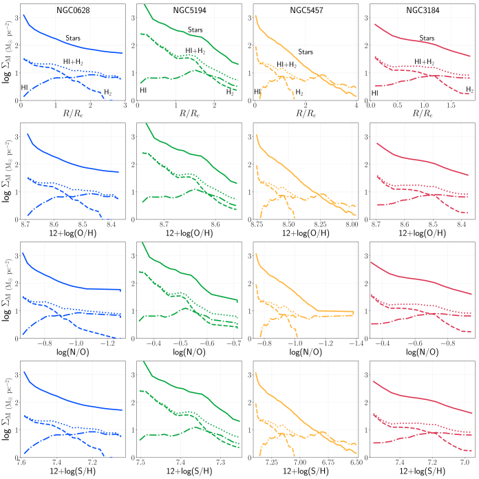
Figure 16.— Mass surface density profiles for different components of the first four CHAOS galaxies versus galactocentric radius (top row), oxygen abundance (middle row), and N/O abundance (bottom row). Values for 12+log(O/H) and log(N/O) are from the linear fits plotted in Figures 6 and 9. Stellar mass profiles are plotted as solid lines and decrease with increasing radius. Molecular H₂ gas profiles are plotted as dashed lines and also generally decrease outward. Atomic H I gas profiles are plotted as dot-dashed lines, intersecting the H₂ trends at unique points in each galaxy. Total H I$+$H₂ gas is shown by the dotted line.

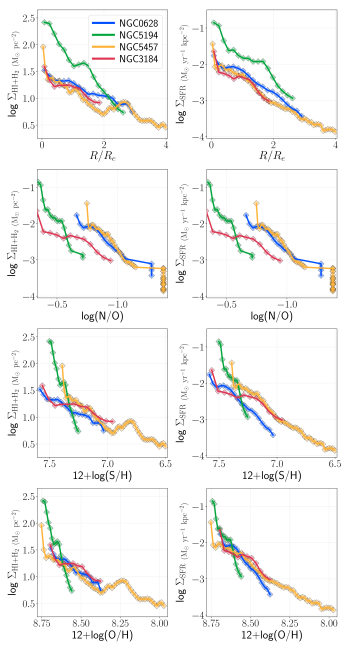
Figure 17.— Left: Total gas mass surface density profiles for the four CHAOS galaxies as scaled by disk effective radius (top), N/O abundance (second), sulfur abundance (third), and oxygen abundance (bottom). These profiles are dominated by the H₂ gas for most of the disk. Right: Total star formation rate surface density profiles versus radius and abundance trends. The right and left columns of panels show the observed increase in local star formation rate with increasing H₂ mass surface density, which drives the increasing abundance trends.

C.2. Profile Comparisons for CHAOS Galaxies

The derived mass surface densities for various galaxy components (i.e., stars, H I, H₂) are plotted in Figure 16 for the CHAOS sample. As expected for an interacting galaxy, the H₂ profile of NGC 5194 is different from the other three galaxies as it both dominates the gas profile and makes up a larger fraction of the total galaxy mass. We find that the stellar and gas mass surface density profiles of the other three non-interacting galaxies to look similar, with H₂ more prominent in the inner $\sim 1R_{e}$ of the disk, H I dominating the outer disk, and the stellar mass roughly following the total gas mass ($M_{gas}=M_{\rm HI}+M_{{\rm H}_{2}}$) for $R_{g}/R_{e}<2$.

We show the total gas mass surface density profiles, which are dominated by the H₂ gas for most of the disk, versus both radius and elemental abundances (O, N, and S ) in the left column of Figure 17. Interestingly, while we find the stellar mass and gas mass surface density profiles of individual galaxies to be offset from one another when plotted versus their N/O profiles, the shift is minimal for the O/H and S/H trends. Since the decline of H₂ gas mass with radius corresponds to a decreasing star formation rate (as shown in the right column of Figure 17) and star formation efficiency, this could indicate that the H₂ mass surface density plays the leading role in the stellar and subsequent chemical evolution of these galaxies.

C.3. Local Scaling Relations

Rosales-Ortega et al. (2012), using IFU spectroscopy from the PINGS (Rosales-Ortega et al., 2010) and CALIFA surveys, reported the first local mass-metallicity (M–Z) scaling relationship of H II regions in spiral galaxies, with a secondary dependence on the equivalent width of H$\alpha$ (a proxy from SFR). This local M–Z–EW(H$\alpha$) relationship is the logical product of inside-out disk growth and the dependence of SFR on mass. While the more widely known fundamental M–Z–SFR global relationship (Mannucci et al., 2010) has been explained by galaxy growth via the accretion of cold gas that is altered by feedback of gaseous inflows and outflows, the local M–Z–SFR relationship allows us to explore physical parameters that may be regulating the growth and chemical evolution within spiral disks.

The stellar mass surface density ($\Sigma_{{\rm M}_{\odot}}$) radial profiles are reproduced for the four CHAOS galaxies in the first panel of Figure 18. We fit a polynomial to the $\Sigma_{{\rm M}_{\odot}}$–$R_{e}$ (Figure 18) and $\Sigma_{\rm SFR}$–$R_{e}$ trend of each galaxy. These fits are then used to plot the stellar mass surface densities corresponding to the observed O/H and N/O abundances of the CHAOS H II regions. The $\Sigma_{{\rm M}_{\odot}}$–O/H and $\Sigma_{{\rm M}_{\odot}}$–N/O trends are plotted in the middle and right panels of Figure 18, respectively, and color-coded by SFR surface density ($\Sigma_{\rm SFR}$). Since SFR is known to depend in stellar mass, the vertical color gradient seen for the SFR in the $\Sigma_{{\rm M}_{\odot}}$–O/H is expected. However, in the $\Sigma_{{\rm M}_{\odot}}$–N/O relationship, not only is the scatter significantly reduced relative to the O/H trend, but SFR also appears to increase along the N/O gradient.

The metallicity-surface density relationship may reflect fundamental similarities in the evolution of non-barred, non-interacting spiral galaxies. For example, Ryder (1995) argues for a galaxy evolution model that includes self-regulating star formation, where energy injected into the ISM by newly-formed stars inhibits further star formation. These models were able to successfully reproduce the observed correlations between surface brightness and SFR (Dopita & Ryder, 1994) and surface mass density (e.g., Phillipps & Edmunds, 1991; Ryder, 1995; Garnett et al., 1997). The current work supports the idea that stellar mass surface density is a fundamental parameter governing spiral galaxy evolution, and is particularly important for the relative timescales involved in N/O production.

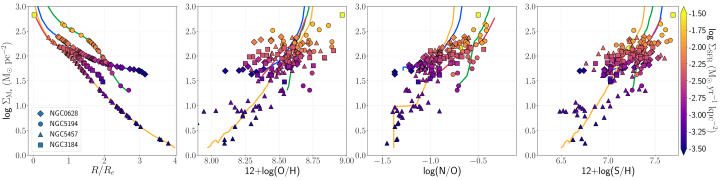
Figure 18.— Left: stellar mass surface densities for the CHAOS sample versus galactocentric radius where the colored lines represent the average profile of each galaxy. Second: the local M–Z–SFR relationship. For each observed data point $x$, we plot the fit log $\Sigma{\rm M}_{\star}(R_{x})$ versus the measured 12+log(O/H)_x, color-coded by the its log $\Sigma{\rm SFR}(R_{x})$ value. The large spread is due to the real scatter in observed O/H. Third: the local M–N/O–SFR relationship. This panel shows the stellar mass surface density trend, similar to the second panel, but versus measured N/O, forming a tight correlation. Right: the local M–S/H–SFR relationship.

References

- Asplund et al. (2009) Asplund, M., Grevesse, N., Sauval, A. J., & Scott, P. 2009, ARA&A, 47, 481
- Bacon et al. (2010) Bacon, R., Accardo, M., Adjali, L., et al. 2010, in Society of Photo-Optical Instrumentation Engineers (SPIE) Conference Series, Vol. 7735, Proc. SPIE, 773508
- Baron et al. (2007) Baron, E., Branch, D., & Hauschildt, P. H. 2007, ApJ, 662, 1148, doi: 10.1086/517961
- Belfiore et al. (2017) Belfiore, F., Maiolino, R., Tremonti, C., et al. 2017, MNRAS, 469, 151, doi: 10.1093/mnras/stx789
- Berg et al. (2018) Berg, D. A., Erb, D. K., Auger, M. W., Pettini, M., & Brammer, G. B. 2018, ApJ, 859, 164
- Berg et al. (2019) Berg, D. A., Erb, D. K., Henry, R. B. C., Skillman, E. D., & McQuinn, K. B. W. 2019, ApJ, 874, 93, doi: 10.3847/1538-4357/ab020a
- Berg et al. (2015) Berg, D. A., Skillman, E. D., Croxall, K. V., et al. 2015, ApJ, 806, 16
- Berg et al. (2012) Berg, D. A., Skillman, E. D., Marble, A. R., et al. 2012, ApJ, 754, 98
- Berg et al. (2020) Berg, D. A., et al. 2020
- Binette et al. (2012) Binette, L., Matadamas, R., Hägele, G. F., et al. 2012, A&A, 547, A29
- Bohlin (2014) Bohlin, R. C. 2014, AJ, 147, 127, doi: 10.1088/0004-6256/147/6/127
- Bolatto et al. (2013) Bolatto, A. D., Wolfire, M., & Leroy, A. K. 2013, ARA&A, 51, 207, doi: 10.1146/annurev-astro-082812-140944
- Bose & Kumar (2014) Bose, S., & Kumar, B. 2014, ApJ, 782, 98
- Bresolin et al. (2016) Bresolin, F., Kudritzki, R.-P., Urbaneja, M. A., et al. 2016, ApJ, 830, 64, doi: 10.3847/0004-637X/830/2/64
- Bruzual & Charlot (2003) Bruzual, G., & Charlot, S. 2003, MNRAS, 344, 1000
- Bryant et al. (2015) Bryant, J. J., Owers, M. S., Robotham, A. S. G., et al. 2015, MNRAS, 447, 2857, doi: 10.1093/mnras/stu2635
- Bundy et al. (2015) Bundy, K., Bershady, M. A., Law, D. R., et al. 2015, ApJ, 798, 7, doi: 10.1088/0004-637X/798/1/7
- Chisholm et al. (2019) Chisholm, J., et al. 2019, ApJ
- Cluver et al. (2017) Cluver, M. E., Jarrett, T. H., Dale, D. A., et al. 2017, ApJ, 850, 68, doi: 10.3847/1538-4357/aa92c7
- Colombo et al. (2014) Colombo, D., Meidt, S. E., Schinnerer, E., et al. 2014, ApJ, 784, 4, doi: 10.1088/0004-637X/784/1/4
- Coziol et al. (1999) Coziol, R., Reyes, R. E. C., Considère, S., Davoust, E., & Contini, T. 1999, A&A, 345, 733
- Crockett et al. (2006) Crockett, N. R., Garnett, D. R., Massey, P., & Jacoby, G. 2006, ApJ, 637, 741
- Croxall et al. (2015) Croxall, K. V., Pogge, R. W., Berg, D. A., Skillman, E. D., & Moustakas, J. 2015, ApJ, 808, 42
- Croxall et al. (2016) —. 2016, ApJ, 830, 4
- Curti et al. (2017) Curti, M., Cresci, G., Mannucci, F., & others. 2017, MNRAS, 465, 1384
- Dale (2009) Dale, D. A., e. a. 2009, ApJ, 703, 517
- De Robertis et al. (1987) De Robertis, M. M., Dufour, R. J., & Hunt, R. W. 1987, JRASC, 81, 195
- de Vaucouleurs et al. (1991) de Vaucouleurs, G., de Vaucouleurs, A., Corwin, Jr., H. G., et al. 1991, in Third Reference Catalogue of Bright Galaxies. Volume I: Explanations and references. Volume II: Data for galaxies between 0h and 12h. Volume III: Data for galaxies between 12h and 24h., by de Vaucouleurs, G.; de Vaucouleurs, A.; Corwin, H. G., Jr.; Buta, R. J.; Paturel, G.; Fouqué, P.. Springer, New York, NY (USA), 1991, 2091 p., ISBN 0-387-97552-7, Price US$ 198.00. ISBN 3-540-97552-7, Price DM 448.00. ISBN 0-387-97549-7 (Vol. I), ISBN 0-387-97550-0 (Vol. II), ISBN 0-387-97551-9 (Vol. III).
- Dopita & Ryder (1994) Dopita, M. A., & Ryder, S. D. 1994, ApJ, 430, 163, doi: 10.1086/174390
- Edmunds & Pagel (1984) Edmunds, M. G., & Pagel, B. E. J. 1984, MNRAS, 211, 507
- Egusa et al. (2009) Egusa, F., Kohno, K., Sofue, Y., Nakanishi, H., & Komugi, S. 2009, ApJ, 697, 1870
- Erb et al. (2010) Erb, D. K., Pettini, M., Shapley, A. E., et al. 2010, ApJ, 719, 1168
- Esteban et al. (2009) Esteban, C., Bresolin, F., Peimbert, M., et al. 2009, ApJ, 700, 654
- Fernandes et al. (2005) Fernandes, I. F., Gruenwald, R., & Viegas, S. M. 2005, MNRAS, 364, 674
- Ferrarese et al. (2000) Ferrarese, L., Ford, H. C., Huchra, J., et al. 2000, ApJS, 128, 431, doi: 10.1086/313391
- Filippenko (1982) Filippenko, A. V. 1982, PASP, 94, 715
- García-Rojas et al. (2013) García-Rojas, J., Peña, M., Morisset, C., et al. 2013, A&A, 558, A122, doi: 10.1051/0004-6361/201322354
- Garnett (1990) Garnett, D. R. 1990, ApJ, 363, 142
- Garnett (1992) Garnett, D. R. 1992, AJ, 103, 1330
- Garnett (2002) Garnett, D. R. 2002, ApJ, 581, 1019
- Garnett & Shields (1987) Garnett, D. R., & Shields, G. A. 1987, ApJ, 317, 82
- Garnett et al. (1997) Garnett, D. R., Shields, G. A., Skillman, E. D., Sagan, S. P., & Dufour, R. J. 1997, ApJ, 489, 63
- Groh et al. (2019) Groh, J. H., Ekström, S., Georgy, C., et al. 2019, arXiv e-prints. https://arxiv.org/abs/1904.04009
- Hägele et al. (2006) Hägele, G. F., Pérez-Montero, E., Díaz, Á. I., Terlevich, E., & Terlevich, R. 2006, MNRAS, 372, 293
- Heger et al. (2003) Heger, A., Fryer, C. L., Woosley, S. E., Langer, N., & Hartmann, D. H. 2003, ApJ, 591, 288, doi: 10.1086/375341
- Henry et al. (2000) Henry, R. B. C., Edmunds, M. G., & Köppen, J. 2000, ApJ, 541, 660
- Henry et al. (2006) Henry, R. B. C., Nava, A., & Prochaska, J. X. 2006, ApJ, 647, 984
- Ho et al. (2015) Ho, I.-T., Kudritzki, R.-P., Kewley, L. J., et al. 2015, MNRAS, 448, 2030, doi: 10.1093/mnras/stv067
- Ho et al. (2018) Ho, I. T., Meidt, S. E., Kudritzki, R.-P., et al. 2018, A&A, 618, A64, doi: 10.1051/0004-6361/201833262
- Ho et al. (2017) Ho, I.-T., Seibert, M., Meidt, S. E., et al. 2017, ApJ, 846, 39, doi: 10.3847/1538-4357/aa8460
- Hummer & Storey (1987) Hummer, D. G., & Storey, P. J. 1987, MNRAS, 224, 801
- Jang & Lee (2017) Jang, I. S., & Lee, M. G. 2017, ApJ, 836, 74, doi: 10.3847/1538-4357/836/1/74
- Jarrett et al. (2013) Jarrett, T. H., Masci, F., Tsai, C. W., et al. 2013, AJ, 145, 6, doi: 10.1088/0004-6256/145/1/6
- Jiménez-Donaire et al. (2017) Jiménez-Donaire, M. J., Cormier, D., Bigiel, F., et al. 2017, ApJ, 836, L29, doi: 10.3847/2041-8213/836/2/L29
- Kelly (2007) Kelly, B. C. 2007, ApJ, 665, 1489
- Kennicutt et al. (2003a) Kennicutt, Jr., R. C., Armus, L., Bendo, G., et al. 2003a, PASP, 115, 928
- Kennicutt et al. (2003b) Kennicutt, Jr., R. C., Bresolin, F., & Garnett, D. R. 2003b, ApJ, 591, 801
- Kewley & Ellison (2008) Kewley, L. J., & Ellison, S. L. 2008, ApJ, 681, 1183
- Kreckel et al. (2018) Kreckel, K., Faesi, C., Kruijssen, J. M. D., et al. 2018, ApJ, 863, L21
- Krumholz & Ting (2018) Krumholz, M. R., & Ting, Y.-S. 2018, MNRAS, 475, 2236, doi: 10.1093/mnras/stx3286
- Leroy et al. (2009) Leroy, A. K., Walter, F., Bigiel, F., et al. 2009, AJ, 137, 4670, doi: 10.1088/0004-6256/137/6/4670
- Leroy et al. (2013) Leroy, A. K., Walter, F., Sandstrom, K., et al. 2013, AJ, 146, 19, doi: 10.1088/0004-6256/146/2/19
- Leroy et al. (2019) Leroy, A. K., et al. 2019, ApJ
- Liu et al. (2001) Liu, X.-W., Luo, S.-G., Barlow, M. J., Danziger, I. J., & Storey, P. J. 2001, MNRAS, 327, 141, doi: 10.1046/j.1365-8711.2001.04676.x
- Luridiana et al. (2012) Luridiana, V., Morisset, C., & Shaw, R. A. 2012, in IAU Symposium, Vol. 283, IAU Symposium, 422–423
- Luridiana et al. (2015) Luridiana, V., Morisset, C., & Shaw, R. A. 2015, A&A, 573, A42
- Maiolino & Mannucci (2019) Maiolino, R., & Mannucci, F. 2019, A&A Rev., 27, 3, doi: 10.1007/s00159-018-0112-2
- Mannucci et al. (2010) Mannucci, F., Cresci, G., Maiolino, R., Marconi, A., & Gnerucci, A. 2010, MNRAS, 408, 2115, doi: 10.1111/j.1365-2966.2010.17291.x
- McCall (1982) McCall, M. L. 1982, PhD thesis, THE UNIVERSITY OF TEXAS AT AUSTIN.
- McQuinn et al. (2017) McQuinn, K. B. W., Skillman, E. D., Dolphin, A. E., Berg, D., & Kennicutt, R. 2017, AJ, 154, 51, doi: 10.3847/1538-3881/aa7aad
- Moustakas et al. (2010) Moustakas, J., Kennicutt, R. C., J., Tremonti, C. A., et al. 2010, ApJS, 190, 233
- Muñoz-Mateos et al. (2009) Muñoz-Mateos, J. C., Gil de Paz, A., Zamorano, J., et al. 2009, ApJ, 703, 1569
- Nava et al. (2006) Nava, A., Casebeer, D., Henry, R. B. C., & Jevremovic, D. 2006, ApJ, 645, 1076
- Nicholls et al. (2017) Nicholls, D. C., Sutherland, R. S., Dopita, M. A., Kewley, L. J., & Groves, B. A. 2017, MNRAS, 466, 4403
- Oke (1990) Oke, J. B. 1990, AJ, 99, 1621
- Pagel & Edmunds (1981) Pagel, B. E. J., & Edmunds, M. G. 1981, ARA&A, 19, 77
- Peña-Guerrero et al. (2012) Peña-Guerrero, M. A., Peimbert, A., & Peimbert, M. 2012, ApJ, 756, L14
- Peimbert & Peimbert (2010) Peimbert, A., & Peimbert, M. 2010, ApJ, 724, 791
- Peimbert (1967) Peimbert, M. 1967, ApJ, 150, 825
- Peimbert & Costero (1969) Peimbert, M., & Costero, R. 1969, Boletin de los Observatorios Tonantzintla y Tacubaya, 5, 3
- Peimbert et al. (1992) Peimbert, M., Torres-Peimbert, S., & Ruiz, M. T. 1992, Revista Mexicana de Astronomia y Astrofisica, 24, 155
- Pérez-Montero et al. (2006) Pérez-Montero, E., Díaz, A. I., Vílchez, J. M., & Kehrig, C. 2006, A&A, 449, 193
- Phillipps & Edmunds (1991) Phillipps, S., & Edmunds, M. G. 1991, MNRAS, 251, 84, doi: 10.1093/mnras/251.1.84
- Pilyugin (1999) Pilyugin, L. S. 1999, A&A, 346, 428
- Pilyugin et al. (2019) Pilyugin, L. S., Grebel, E. K., Zinchenko, I. A., Nefedyev, Y. A., & Vílchez, J. M. 2019, A&A, 623, A122, doi: 10.1051/0004-6361/201834239
- Pilyugin et al. (2009) Pilyugin, L. S., Mattsson, L., Vílchez, J. M., & Cedrés, B. 2009, MNRAS, 398, 485
- Pipino & Matteucci (2009) Pipino, A., & Matteucci, F. 2009, in IAU Symposium, Vol. 258, The Ages of Stars, ed. E. E. Mamajek, D. R. Soderblom, & R. F. G. Wyse, 39–50
- Pogge et al. (2010) Pogge, R. W., Atwood, B., Brewer, D. F., et al. 2010, in Society of Photo-Optical Instrumentation Engineers (SPIE) Conference Series, Vol. 7735, Society of Photo-Optical Instrumentation Engineers (SPIE) Conference Series
- Querejeta et al. (2015) Querejeta, M., Meidt, S. E., Schinnerer, E., et al. 2015, ApJS, 219, 5, doi: 10.1088/0067-0049/219/1/5
- Rigby et al. (2015) Rigby, J. R., Bayliss, M. B., Gladders, M. D., & others. 2015, ApJ, 814, L6