Tutorial on electromagnetic nonreciprocity
and its origins

Abstract

This tutorial provides an intuitive and concrete description of the phenomena of electromagnetic nonreciprocity that will be useful for readers with engineering or physics backgrounds. The notion of time reversal and its different definitions are discussed with special emphasis to its relationship with the reciprocity concept. Starting from the Onsager reciprocal relations generally applicable to many physical processes, we present the derivation of the Lorentz theorem and discuss other implications of reciprocity for electromagnetic systems. Next, we identify all possible routes towards engineering nonreciprocal devices and analyze in detail three of them: Based on external bias, based on nonlinear and time-variant systems. The principles of the operation of different nonreciprocal devices are explained. We address the similarity and fundamental difference between nonreciprocal effects and asymmetric transmission in reciprocal systems. In addition to the tutorial description of the topic, the manuscript also contains original findings. In particular, general classification of reciprocal and nonreciprocal phenomena in linear bianisotropic media based on the space- and time-reversal symmetries is presented. This classification serves as a powerful tool for drawing analogies between seemingly distinct effects having the same physical origin and can be used for predicting novel electromagnetic phenomena. Furthermore, electromagnetic reciprocity theorem for time-varying systems is derived and its applicability is discussed.

I Introduction

The notion of reciprocity and nonreciprocity is a fundamental scientific concept, important in many different branches of physics, chemistry, and engineering. In the general sense, electromagnetic nonreciprocity implies that the fields created by a source at the observation point are not the same compared to the case when the source and observation point are interchanged. Nonreciprocal systems are essential for applications where one-way propagation is required [1, § 13.3],[2, § 9.4]: Radars using a single antenna for transmitting and receiving at the same time, suppression of destabilizing reflections in lasers, isolating signals from a power supply, etc.

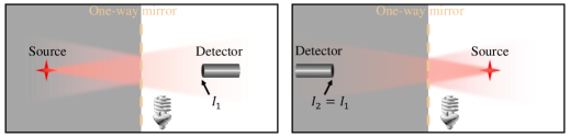
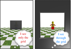
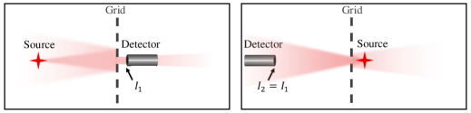
Figure 1: Examples from everyday life which resemble nonrecirpocal light propagation. In fact, reciprocity is preserved in both examples. (a) Two observers are separated by a one-way mirror (silver coated glass). The blue observer is located on the bright side, illuminated by a bulb. The strong light from the bulb obscures the dimmed light coming from the red observer: The blue observer sees his own image. Meanwhile, the red observer clearly sees through the mirror. (b) A thought experiment proving reciprocity of the one-way mirror. Grey and white backgrounds denote dark and bright regions, respectively. Light intensities $I_{1}$ and $I_{2}$ measured by the detector at the two locations are equal (the detector measures only light from the source and not from the bulb). (c) Images seen by the two observers standing at the two sides of a metal grid fence at large (left figure) and very short (right figure). The blue observer sees the red observer, but not vice versa. (d) A thought experiment proving reciprocity of the grid fence.

Although there is a rigorous definition of reciprocity breaking, the concept of nonreciprocity is not trivial and may be easily interpreted erroneously. Consider an example from our everyday life, commercialized one-way mirrors [3] (used for surveillance or as reflective windows in buildings) which exhibit fictitious one-way wave propagation. In fact, such mirrors are completely reciprocal and their operation is based on the brightness contrast at the two sides of the mirror. The observer located on the bright side will receive dimmed light coming from the objects in the dark, but this image will be strongly obscured by the bright reflection of the observer himself (see Fig. 1). Nevertheless, reciprocity of this system can be proven by replacing observers with a point light source and a detector, as shown in Fig. 1. The detected signal from the source (excluding the signal from the external bulb) remains the same even after interchanging the positions of the source and detector. Another example of fictitious perception of nonreciprocity is a metal-grid fence: An observer standing at the near proximity of the fence sees another observer, standing at the opposite side far from the fence, more clear than contrariwise (see Fig. 1). Such effect occurs due to the contrast in the viewing angles of the two observers. Obviously, the fence is reciprocal, which can be verified by positioning a light source and a light detector in place of the observers (see Fig. 1). Interchanging the locations of the source and the detector will not modify the signal from the source measured by the detector. In a very simplistic way, one could define reciprocity of an optical system as “if I can see your eyes, then you can see mine”, which holds for this example (both observers see eyes of one another equally well). However, it is obvious that such definition is not general and fails for the previous example system with so-called one-way mirrors.

These examples evidently demonstrate that the rigorous definition of electromagnetic nonreciprocity might come to drastic contradictions with the simplistic commonplace sense. Importantly, although reciprocal systems, such as one-way mirrors, are much easier for deployment and use than the truly nonreciprocal counterparts, they cannot provide truly nonreciprocal effects.

The concept of reciprocity (nonreciprocity) has a long history. Probably, the earliest theoretical works about this concept were developed by Stokes in 1849 [4] and Helmholtz in 1856 [5] for light waves. At the same time, the reciprocity property was postulated for thermoelectric phenomena by Thomson (Lord Kelvin) in 1854 [6]. In 1860 Kirchhoff reformulated the reciprocity principle for thermal radiation [7]. Rayleigh described this principle for acoustics in his book published in 1878 [8]. Hendrik Lorentz came up with his famous electromagnetic reciprocity theorem in 1896 [9]. The fundamental relation between the time-reversal invariance on microscopic dynamic equations and reciprocity in dissipative systems was realized by L. Onsager [10, 11] and developed and extended by H. Casimir [12] to electromagnetic systems and to response functions of materials under influence of external bias fields.

Conventional route for achieving electromagnetic nonreciprocity (breaking reciprocity) is based on the magneto-optical effect [13, 14, 15, 16, 17, 1, 18, 19] which implies asymmetric wave propagation through a medium (e.g., ferrimagnetic material) in the presence of a static magnetic field. Although nonreciprocal systems at microwaves have been extensively developed in the middle of the twentieth century, efficient and compact nonreciprocal components operating at optical frequencies (natural materials exhibit weak magneto-optical effects in optics since both the cyclotron frequency of free electrons and the Larmor frequency of spin precession of bound electrons are typically in the microwave range [20, p. 571],[2, § 9.1],[15, § 79]) are yet to be found. During the last decade, several alternative routes towards realization of nonreciprocal wave propagation in optics have been actively developed. Among them the most promising are based on nonlinear [21, 22, 23, 24, 25, 26, 27, 28, 29, 30, 31, 32, 33, 34, 35, 36, 37, 38, 39, 40, 41, 42, 43, 44, 45, 46, 47, 48, 49, 50, 51, 52, 53] and active [54, 55, 56, 57] materials as well as materials whose properties are modulated in time by some external source [58, 59, 60, 61, 62, 63, 64, 65, 66, 67, 68, 69, 70, 71, 72, 73, 74, 75, 76, 77, 78, 79, 80, 81, 82, 83, 84, 85, 86]. Comprehensive classification of nonreciprocal systems and their theoretical description can be found in recent review papers on this topic [87, 88, 89, 90, 91, 92, 93, 94, 95, 96, 97].

In this tutorial, we present the reciprocity and nonreciprocity notions in the educational manner, accessible for the readers without solid background in this field. We explain the origins of different nonreciprocal effects and demonstrate how they are related to time-reversal and space-reversal symmetries of the system. The paper also provides classification of non-reciprocal phenomena in most general bianisotropic scatterers and media. It is important to note that throughout the paper time harmonic oscillations in the form ${\rm e}^{+j\omega t}$ are assumed according to the conventional electrical engineering notations [98, 2].

II Time reversal in electrodynamics

II-A Time reversal definition and Loschmidt’s paradox

The concept of electromagnetic reciprocity is closely related to that of the time-reversal symmetry of Maxwell’s equations. The same symmetry property of field equations leads also to time-reversability of physical processes in lossless systems. Nevertheless, the concepts of reciprocity and time reversal of physical processes have fundamental differences and, therefore, should be distinguished. For the subsequent description, we start our discussion with the concept of time reversal.

One of the fundamental questions in physics is “Can the direction of time flow be determined?” [99]. Our everyday experience suggests that it can be. When we mix up two substances, we know that we cannot reverse the process of mixing and separate the substances from the mixture. When we see a video of some macroscopic physical process, in most cases, we can definitely say whether it is played forward or backward. Nevertheless, the question about the time flow is not related to our daily experience, and it required several generations of physicists to obtain the answer. This question is directly linked to another one: “Are all physical laws invariant under time reversal?” Conventionally, a physical process is called time-reversal invariant or reversible if its evolution in the backward direction (think about the reversed video of the original process) is also a realistic process [100, § 2.3]. That is, this evolution also satisfies the dynamic equations. For example, the played-backward process of a ball scattering on the billiard table looks as realistic as the direct process (assuming elastic ball collisions).

An equivalent definition of a time-reversal invariant process was formulated by H. Casimir [101] (see also [102]): “If a system of particles and fields moves in a certain way during the period $0<t<t_{0}$ and if at the moment $t_{0}$ we would invert all velocities, currents, magnetic fields and so on, then the system retraces its steps: At the time $2t_{0}$ particle coordinates and fields are what they were at $t=0$, at a time $2t_{0}-t$ the situation is what it was at $t$ ”. Figure 2 illustrates this definition by plotting a coordinate $r$ and velocity projection $v$ of some particle as functions of time $t$. The initial particle motion is shown in red. At moment $t_{0}$, the speed of the particle flips its direction, while its coordinate remains the same. This arrangement is equivalent to playing the video of the motion backward. The blue curve shows the reversed particle motion. At moment $2t_{0}$, the particle returns to its initial position as at $t=0$ with the same speed but in the opposite direction.

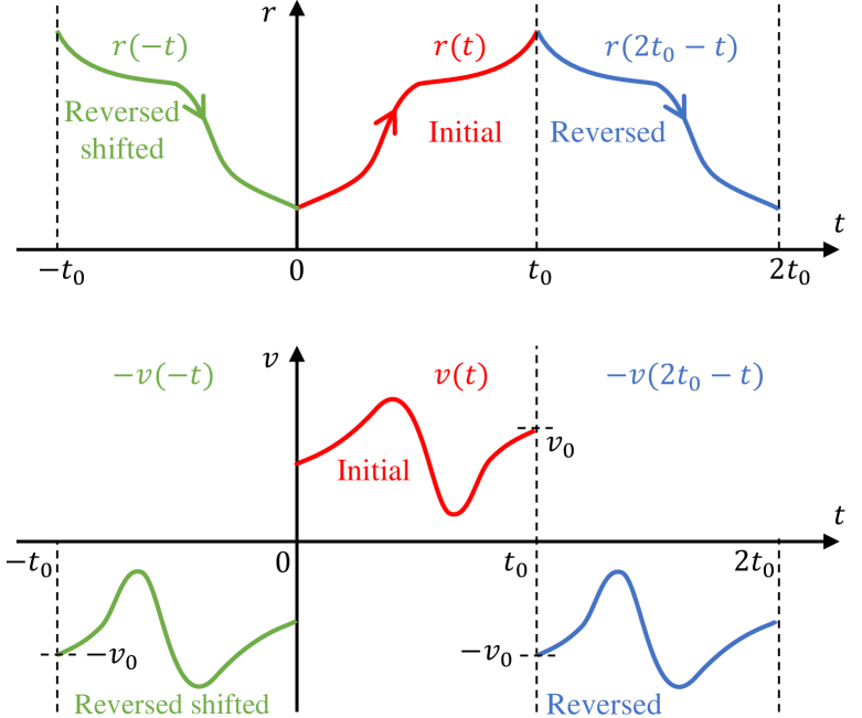
Figure 2: Time reversal of the coordinate function of an arbitrary object (a billiard ball in this example). Although in the reversed process the time arrow direction does not change (${\rm d}t>0$), the displacement ${\rm d}r(t)$ and the derivative of the coordinate (velocity) in the reversed system flip the signs.

The green curve in the plots of Fig. 2 depicts the curve for the reversed motion shifted along the time axis by $-2t_{0}$. The blue and green curves are physically identical and correspond to the same motion due to the uniformity of time (the choice of time origin $t=0$ is a matter of convenience). Comparing the initial motion, red curve, with the reversed shifted motion, green curve, one can see that the curves are identical mirrors of one another with respect to $t=0$ (the velocity curve has an additional flip of the direction). This is why the physical notion of time reversal is conventionally written mathematically as $t\rightarrow-t$ [101, 102, 103, 104],[105, § 1.9.2],[106, Ch. 8],[107, § 4.1.2],[108, p. 270],[90]. If the equations describing the process do not change under substitution $t\rightarrow-t$, the process is called time-reversal invariant. As one can see from Fig. 2, the coordinate of time-reversed process is related to that of the original process as $T\{r(t)\}=r(-t)$, while the corresponding velocities are related by $T\{v(t)\}=-v(-t)$. Furthermore, time reversal operation does not change the sign of differential ${\rm d}t$ (the time arrow direction remains the same), while it flips the sign of the infinitesimal displacement ${\rm d}r(t)$. One can also note from the bottom panel of Fig. 2 that the infinitesimal increase of the velocity ${\rm d}v(t)$ does not change sign under time reversal (compare the slopes of the red curve at $t_{0}$ and green curve at $-t_{0}$). Therefore, the acceleration of an object $a={\rm d}v/{\rm d}t$ is an even function with respect to the time-reversal operation.

Although in this tutorial, as well as in the majority of books in the literature, the two definitions of time reversal given above are likened, it was pointed out in [109] that they can yield different results for some special objects in spacetime. The first definition of time reversal based on inversion of all velocities by H. Casimir is sometimes referred to as “active” [109, 110], since the transformation is applied directly on the objects motion. The second definition given by simple flipping of time $t\rightarrow-t$ also corresponds to the “active” scenario. One can also think of a “passive” time reversal for which the transformation does not act on the objects but rather on the time axis. For the sake of exposition completeness, it should be mentioned that there exist alternative definitions of time reversal, such as [111, Ch. 3] [112, Ch. 1], which are not generally accepted in the physics community [113].

All the physical laws, with the only exception of those corresponding to weak interactions, are governed by the equations which are symmetric under time reversal. However, our daily experience tells us that most physical processes, governed by the very same physical laws, are irreversible in time. Moreover, our experience is also supported by the second law of thermodynamics expressed as ${\rm d}S/{\rm d}t\geq 0$ which says that any closed physical system cannot evolve from a disordered to a more ordered state (e.g., reversing a process of dye mixing would violate this law). This contradiction of irreversible processes which are governed by time-reversible physical laws was pointed out by J. Loschmidt in 1877 [114] and was named subsequently as Loschmidt’s paradox. An elegant explanation of the paradox can be found in [100, Ch. 2]. It is based on the fact that a physical process is not only determined by the physical laws, but it also depends on the initial conditions.

Figure 3 illustrates resolving the paradox. Consider a closed box with gas and assume that at $t=0$ all its molecules occupied only a small region in the corner of the box, as is shown in Fig. 3. The red arrows indicate the velocities of the molecules. After some time $t_{0}$, the molecules will spread somewhat uniform inside the box.

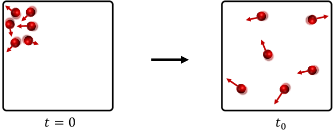
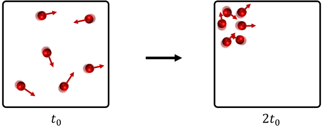
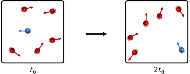
Figure 3: Gas molecules in a closed box. (a) Evolution of the molecules distribution from an ordered state to a disordered state. The arrows indicate the velocity directions. (b) Time reversal of the process in (a) with correct microscopic initial conditions (positions of the molecules are unchanged, while velocities are reversed). (c) Time reversal of the process in (a) with macroscopic initial conditions. Microscopic conditions are not fully satisfied, the blue molecule indicate the wrong initial state.

Time reversal of the process in Fig. 3 requires fulfilment of the correct initial conditions. Let us assume that we are able to position all the molecules anywhere in the box and launch them at some moment $t_{0}$ with desired initial velocities. If we choose the position of the molecules as in the right illustration of Fig. 3 and launch them with the same velocities but in the opposite directions, then after time period $t_{0}$ the molecules would come back exactly to the initial ordered state (see Fig. 3). In other words, the process reversal would be possible if we were able to ensure the microscopic initial conditions (position and velocity) for each molecule. In practice, assigning correct initial conditions even for a few molecules is a complicated engineering problem, therefore, for systems with large numbers of molecules the only parameters that we control are statistical ones, such as the mean speed and the mean free path. These statistical parameters are related to macroscopic pressure and temperature. If we try to reverse the process in Fig. 3 by satisfying only the macroscopic initial conditions (for example, by wrongly assigning velocity of one of the molecules, as is shown in Fig. 3), the gas would not come back to the initial state and, moreover, the new state would be drastically different from the initial one. The probability that by satisfying the macroscopic initial conditions we also ensure by chance the microscopic ones is proportional to $n^{-N}$, where $N$ is the number of molecules in the closed box and $n$ is the number of possible states of each molecule [10, p. 414]. Thus, due to the exponentially decreasing probability, all macroscopic processes appear to us irreversible.

A given macroscopic (thermodynamic) state is consistent with the great variety of possible microscopic states. Strictly speaking, any process may be reversed since it may happen that the macroscopic initial conditions were chosen exactly satisfying the microscopic initial conditions. However, the probability of this event will be incredibly small, exponentially decreasing with the number of particles and their degrees of freedom. This reasoning explains why most processes which we observe are irreversible: Mixing substances, cracking objects, combustion, and even lossy phenomena. Nevertheless, although it sounds somewhat bizarre, all these processes are reversible under time reversal (with correct microscopic initial conditions) since they are governed by time-symmetric physical laws.

Until the middle of the twentieth century, scientists could not find any exception among physical laws that would be asymmetric with respect to time reversal. Moreover, the discovery of the CPT theorem in quantum field theory [115], stating that all physical laws are symmetric under the simultaneous transformations of charge conjugation (C), parity transformation (P), and time reversal (T), became an additional argument for the universality of time reversal symmetry. However, in the late 1950s a violation of parity symmetry by phenomena that involve the weak force was reported. Starting from 1964, a series of experiments on decay of K-meson has demonstrated that even CP symmetry can be violated. Assuming that the CPT theorem is fundamental, the latter result meant automatically that time symmetry of the weak interactions can be broken. Coming back to the question in the beginning of this section, we now see that the direction of time in fact can be determined.

II-B Time reversal symmetry of Maxwell’s equations

It is reasonable to assume that under time reversal, microscopic electrodynamic quantities either do not change (time-reversal symmetric or even) or flip sign (time-reversal asymmetric or odd). Moreover, it is reasonable to assume that the electric charge $q$, charge density $\rho$, and coordinate $r$ do not change under time reversal. Under this assumption, speed ${\bf v\mit}$ and electric current ${\bf j\mit}$ are odd with respect to time reversal (see also Fig. 2). The force is proportional to the acceleration ${\bf a\mit}$ and, therefore, is symmetric. Next, it is easy to determine the time-reversal properties of most electrodynamic microscopic quantities. The electric field $\tilde{{\bf e\mit}}$, being proportional to the force acting on a unit charge, is time-reversal even. From the formula for the Lorentz force $\tilde{{\bf F\mit}}=q\tilde{{\bf e\mit}}+q\tilde{{\bf v\mit}}\times\tilde{{\bf b\mit}}$, one can deduct that magnetic field $\tilde{{\bf b\mit}}$ must be time-reversal odd (multiplication of speed and magnetic field must be time-reversal even). Note that hereafter we use tilde symbol “$\sim$” above physical quantities defined in the time domain. The frequency-domain version of these quantities will be written without tilde.

We see that under these assumptions the microscopic Maxwell’s equations

$$\begin{array}[]{c}\displaystyle\nabla\times\tilde{\mathbf{e}}=-\frac{\partial\tilde{\mathbf{b}}}{\partial t},\qquad\nabla\cdot\tilde{\mathbf{b}}=0\\ \displaystyle\nabla\times\tilde{\mathbf{b}}=\frac{1}{c^{2}}\frac{\partial\tilde{\mathbf{e}}}{\partial t}+\mu_{0}\tilde{\mathbf{j}},\qquad\nabla\cdot\tilde{\mathbf{e}}=\tilde{\rho}/\varepsilon_{0}\end{array}$$ (1)

are invariant under time reversal. This conclusion is in agreement with experimental observations about electromagnetic phenomena, most importantly, with the reciprocity principle, which we will discuss in detail. Table I summarizes the time-reversal properties of microscopic electrodynamic quantities.

Physical Quantity	Time Reversal
(microscopic quantities)	Time Reversal
(macroscopic quantities)
Charge density	${\tilde{\rho}}(t)\mapsto+{\tilde{\rho}}(-t)$	${\tilde{\rho}}(t)\mapsto+{\tilde{\rho}}(-t)$
Current density	$\tilde{\mathbf{j}}(t)\mapsto-\tilde{\mathbf{j}}(-t)$	$\tilde{\mathbf{J}}(t)\mapsto-\tilde{\mathbf{J}}(-t)$
Displacement	–	$\tilde{\mathbf{D}}(t)\mapsto+\tilde{\mathbf{D}}(-t)$
Electric field	$\tilde{\mathbf{e}}(t)\mapsto+\tilde{\mathbf{e}}(-t)$	$\tilde{\mathbf{E}}(t)\mapsto+\tilde{\mathbf{E}}(-t)$
Magnetic field	–	$\tilde{\mathbf{H}}(t)\mapsto-\tilde{\mathbf{H}}(-t)$
Magnetic induction	$\tilde{\mathbf{b}}(t)\mapsto-\tilde{\mathbf{b}}(-t)$	$\tilde{\mathbf{B}}(t)\mapsto-\tilde{\mathbf{B}}(-t)$
Magnetization	–	$\tilde{\mathbf{M}}(t)\mapsto-\tilde{\mathbf{M}}(-t)$
Polarization density	–	$\tilde{\mathbf{P}}(t)\mapsto+\tilde{\mathbf{P}}(-t)$
Poynting vector	$\tilde{\mathbf{S}}(t)\mapsto-\tilde{\mathbf{S}}(-t)$	$\tilde{\mathbf{S}}(t)\mapsto-\tilde{\mathbf{S}}(-t)$

TABLE I: Transformation properties of electrodynamic quantities under time reversal

The macroscopic electromagnetic fields are obtained through volume averaging of the microscopic ones. In the macroscopic form, Maxwell’s equations are usually written as

$$\begin{array}[]{c}\displaystyle\nabla\times\tilde{\mathbf{E}}=-\frac{\partial\tilde{\mathbf{B}}}{\partial t},\qquad\nabla\cdot\tilde{\mathbf{B}}=0,\\ \displaystyle\nabla\times\tilde{\mathbf{H}}=\frac{\partial\tilde{\mathbf{D}}}{\partial t}+\tilde{\mathbf{J}}_{\rm ext},\qquad\nabla\cdot\tilde{\mathbf{D}}=\tilde{\rho}_{\rm ext},\end{array}$$ (2)

where $\tilde{\mathbf{E}}$ and $\tilde{\mathbf{B}}$ are the electric field and magnetic flux density averaged over a small macroscopic volume, $\tilde{\mathbf{D}}$ and $\tilde{\mathbf{H}}$ are the electric displacement field and magnetic field, respectively, and $\tilde{\rho}_{\rm ext}$ and $\tilde{\mathbf{J}}_{\rm ext}$ are the averaged external (free) electric charge and current density. Here, the term “external” describes the charges and currents which are not affected by the fields (they are not induced by the electric and magnetic fields governed by this set of Maxwell’s equations, being external to this system). The two latter fields are defined as

$$\tilde{\mathbf{D}}=\varepsilon_{0}\tilde{\mathbf{E}}+\tilde{\mathbf{P}},\qquad\tilde{\mathbf{H}}=\frac{1}{\mu_{0}}\tilde{\mathbf{B}}-\tilde{\mathbf{M}},$$ (3)

where $\tilde{\mathbf{P}}$ and $\tilde{\mathbf{M}}$ are the volume polarization densities of electric and magnetic dipole moments induced in the material. The electric polarization density is defined as $\nabla\cdot\tilde{{\bf P\mit}}=-\tilde{\rho}_{\rm ind}$, where $\tilde{\rho}_{\rm ind}$ stands for the induced (bound) electric charge density. The magnetization is defined by $\nabla\times\tilde{{\bf M\mit}}=\tilde{{\bf J\mit}}_{\rm ind}-\partial\tilde{{\bf P\mit}}/\partial t$ [116, Eq. (2.45)].

Because the process of volume averaging does not involve the time variable, the same property of time-reversal symmetry is true also for the system of macroscopic Maxwell’s equations. This conclusion implies, naturally, the assumption that the time-reversal operation includes inversion of equations which govern also the external charges and currents, $\tilde{\rho}_{\rm ext}$ and $\tilde{\mathbf{J}}_{\rm ext}$, i.e. inversion with correct microscopic initial conditions (see discussion in Section II-A). However, only if the dissipation losses in the system are negligible, then the time-reversal symmetry of field equations may lead to time-reversibility of electromagnetic processes.

II-C Time reversal of material relations

Let us consider time reversal of an arbitrary wave process in a stationary dielectric material. The dielectric is assumed to be isotropic, possibly nonuniform, and its magnetization is zero so that $\tilde{{\bf P\mit}}=\tilde{{\bf P\mit}}({\bf r\mit},t)$ and $\tilde{{\bf M\mit}}=0$. Assuming spatially local response, the volume electric polarization density $\tilde{{\bf P\mit}}$ in the time domain is related to the electric field acting on the material by $\tilde{\mathbf{P}}(t)=\varepsilon_{0}\int_{-\infty}^{t}\tilde{\chi}(t-t^{\prime})\tilde{\mathbf{E}}(t^{\prime}){\rm d}t^{\prime}$, where $\tilde{\chi}$ is the electric susceptibility. Note that the upper integration limit is $t$, rather than $+\infty$ to account for causality of the process. After the standard replacement, the displacement vector can be written as the convolution integral

$$\tilde{\mathbf{D}}(t)=\int_{0}^{\infty}\varepsilon_{0}\tilde{\varepsilon}(\tau)\tilde{\mathbf{E}}(t-\tau){\rm d}\tau,$$ (4)

where $\tilde{\varepsilon}(\tau)=\delta(\tau)+\tilde{\chi}(\tau)$. It is convenient to simplify the integral expression for the displacement vector using the Fourier transform, which yields the well-known material relations for an isotropic dielectric without spatial dispersion:

$${\mathbf{D}}(\omega)=\varepsilon_{0}{\varepsilon}(\omega){\mathbf{E}}(\omega),\qquad{\mathbf{B}}(\omega)=\mu_{0}{\mathbf{H}}(\omega),$$ (5)

where

$${\varepsilon}(\omega)=\int_{0}^{\infty}\tilde{\varepsilon}(\tau){\rm e}^{-j\omega\tau}{\rm d}\tau,$$ (6)

and $\varepsilon_{0}$ and $\mu_{0}$ are the permittivity and permeability of vacuum.

By applying the Fourier transform to both sides of the Maxwell equations (2) and substituting (5), we obtain their frequency-domain version:

$$\begin{array}[]{c}\displaystyle\nabla\times{\mathbf{E}}(\omega,{\bf r\mit})=-j\omega\mu_{0}{\mathbf{H}}(\omega,{\bf r\mit}),\quad\nabla\cdot\left[{\varepsilon}(\omega,{\bf r\mit}){\mathbf{E}}(\omega,{\bf r\mit})\right]=0,\\ \displaystyle\nabla\times{\mathbf{H}}(\omega,{\bf r\mit})=j\omega\varepsilon_{0}{\varepsilon}(\omega,{\bf r\mit}){\mathbf{E}}(\omega,{\bf r\mit}),\quad\nabla\cdot{\mathbf{H}}(\omega,{\bf r\mit})=0,\end{array}$$ (7)

where the free currents and charge densities are assumed to be zero. Using conventional algebraic manipulations, we obtain the following wave equation in terms of the magnetic field:

$$\nabla\times\left[\frac{1}{{\varepsilon}(\omega,{\bf r\mit})}\nabla\times{{\bf H\mit}}(\omega,{\bf r\mit})\right]=\frac{\omega^{2}}{c^{2}}{{\bf H\mit}}(\omega,{\bf r\mit}).$$ (8)

An additional requirement for the magnetic field is dictated by condition $\nabla\cdot{\mathbf{H}}(\omega,{\bf r\mit})=0$. Note that condition $\nabla\cdot\left[{\varepsilon}(\omega,{\bf r\mit}){\mathbf{E}}(\omega,{\bf r\mit})\right]=0$ is satisfied automatically due to Faraday’s law in (7) and the fact that the divergence of a curl is always zero.

Next, let us investigate how time reversal applies to the magnetic field $\tilde{{\bf H\mit}}$ in the frequency domain. The frequency spectrum of the field in the original process is given by the Fourier transform

$${\mathbf{H}}(\omega,{\bf r\mit})=1/(2\pi)\int_{-\infty}^{+\infty}\tilde{{\bf H\mit}}(t,{\bf r\mit}){\rm e}^{-j\omega t}{\rm d}t.$$ (9)

Under time reversal, the field in the time domain transforms as $T\{\tilde{{\bf H\mit}}(t,{\bf r\mit})\}=-\tilde{{\bf H\mit}}(-t,{\bf r\mit})$ (see Table I). The Fourier transform of the field in the reversed process is

$$\begin{array}[]{c}\displaystyle T\{{\mathbf{H}}(\omega,{\bf r\mit})\}=1/(2\pi)\int_{-\infty}^{+\infty}-\tilde{{\bf H\mit}}(-t,{\bf r\mit}){\rm e}^{-j\omega t}{\rm d}t\vspace{1mm}\\ \displaystyle=-1/(2\pi)\int_{-\infty}^{+\infty}\tilde{{\bf H\mit}}(t,{\bf r\mit}){\rm e}^{j\omega t}{\rm d}t.\end{array}$$ (10)

By comparing (9) and (10), we obtain

$$T\{{\mathbf{H}}(\omega,{\bf r\mit})\}=-{\mathbf{H}}(-\omega,{\bf r\mit})=-{\mathbf{H}}^{\ast}(\omega,{\bf r\mit}).$$ (11)

For time-even fields, time reversal results in complex conjugate without the sign flip, i.e. for electric field

$$T\{{\mathbf{E}}(\omega,{\bf r\mit})\}={\mathbf{E}}(-\omega,{\bf r\mit})={\mathbf{E}}^{\ast}(\omega,{\bf r\mit}).$$ (12)

Next, applying time reversal to both sides of (5), we conclude that the time-reversal symmetry of field equations (here, including material relations) dictates the following rule for time-reversal of the complex permittivity:

$$T\left\{{\varepsilon}(\omega)\right\}={\varepsilon}^{*}(\omega).$$ (13)

It should be noted that the same results were reported in [90, § VIII]. The expression in (13) implies that under time reversal lossy media become active and vice versa. This should not be surprising since time reversal involves the global reversal of the process with correct microscopic initial conditions. If the direct process was lossy, in the reversed process, the phonons of the dielectric lattice will oscillate in such a way that their energy will be transformed back into the energy of electromagnetic waves (similarly to the process in Fig. 3). Naturally, this exact process reversal is impossible in practice, due to the vast number of microscopic conditions to be satisfied. We are able to reverse only the macroscopic conditions, sending the wave in the opposite direction without reversing the lattice vibrations. Then the dielectric permittivity will remain lossy and the reversed process will be different from the original one.

The original and time-reversed waves described in the frequency domain by magnetic fields ${\mathbf{H}}(\omega,{\bf r\mit})$ and $T\{{\mathbf{H}}(\omega,{\bf r\mit})\}=-{\mathbf{H}}^{\ast}(\omega,{\bf r\mit})$, respectively, propagate in the opposite directions. This can be shown on the example of plane wave propagation so that ${\mathbf{H}}(\omega,{\bf r\mit})={\bf H\mit}_{0}{\rm e}^{-j{\bf k\mit}(\omega){\bf r\mit}}$, where ${\bf k\mit}(\omega)$ is the wavevector and ${\bf H\mit}_{0}$ denotes real vector. The time-harmonic magnetic field for these two waves would be $\tilde{{\bf H\mit}}(t,{\bf r\mit})={\bf H\mit}_{0}{\rm Re\mit}({\rm e}^{-j{\bf k\mit}{\bf r\mit}}{\rm e}^{j\omega t})$ and $T\{\tilde{{\bf H\mit}}(t,{\bf r\mit})\}=-{\bf H\mit}_{0}{\rm Re\mit}({\rm e}^{j{\bf k\mit}^{\ast}{\bf r\mit}}{\rm e}^{j\omega t})$, respectively. Due to the different signs in front of the wavevectors, the propagation directions of these two waves are opposite. Next, we will discuss in detail time reversal in two different characteristic groups of materials: Dielectric and magneto-optical materials.

II-D Time reversal of wave propagation in a dielectric material

Let the original wave propagation process in a dielectric material with some complex permittivity ${\varepsilon}(\omega,{\bf r\mit})={\varepsilon}^{\prime}-j{\varepsilon}^{\prime\prime}$ be described by wave equation (8) written as

$$\nabla\times\left[\frac{1}{{\varepsilon}(\omega,{\bf r\mit})}\nabla\times{{\bf H\mit}}_{\rm orig}(\omega,{\bf r\mit})\right]=\frac{\omega^{2}}{c^{2}}{{\bf H\mit}}_{\rm orig}(\omega,{\bf r\mit}).$$ (14)

Next, consider wave propagation in the time-reversed version of the dielectric material. Since time reversal implies that all microscopic time-odd quantities flip sign and time-even quantities remain the same, effectively a lossy medium would be transformed into an active one, and vice versa. Mathematically, it means that the time-reversed version of the dielectric is described by complex conjugate of the original permittivity ${\varepsilon}^{\ast}(\omega,{\bf r\mit})$. By applying complex conjugate to both sides of (14) and taking into account (11), it is straightforward to see that the wave solution in the time-reversed medium corresponds to $T\{{{\bf H\mit}}_{\rm orig}\}$. Thus, the original and time-reversed (microscopically) waves propagating in a dielectric material have the same waveform but opposite propagation directions, as illustrated in cells A.1 and B.1 of the table in Fig. 4. Wave function $\tilde{\psi}(t,r)$ in the table represents a general time-even field quantity (magnetic field is time-odd and has an additional sign flip). Cell C.1 shows this function versus time and coordinate. The time-reversed field function is just a mirror copy of the direct field function with respect to the point $t=0$.

It is important to mention that the presented definition of time-reversal symmetry differs from that used in [90, § XII]. In particular, our definition corresponds to microscopic reversal and, therefore, lossy dielectric materials are considered time-reversal symmetric. On the contrary, in [90] the definition is macroscopic, and lossy dielectric materials break time-reversal symmetry.

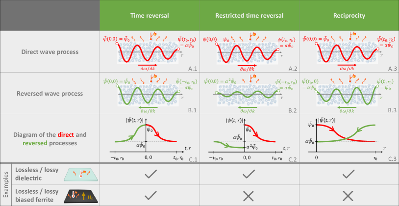
Figure 4: Table comparing the concepts of time reversal, restricted time reversal, and reciprocity for several classes of materials (for simplicity, we assume homogeneous materials). Red and green curves represent the general time-even (e.g., electric field) field function $\psi(t,r)$ of the direct and reversed wave processes, respectively. For a time-odd field function (e.g., magnetic field), the green curves in cells B.1–B.3 must be additionally flipped along the vertical direction.

II-E Time reversal of wave propagation in a magneto-optical material

Magneto-optical materials are materials biased by external or internal static (sometimes, quasi-static) magnetic field, which we denote ${\bf H\mit}_{0}$. The bias field can be created by some external magnet or by exchange interactions of the material itself (like in magnetic crystals), which aligns permanent magnetic moments of atoms. For example, in a magnetized free-electron plasma, owing to electron cyclotron orbiting, the permittivity is described by a second-rank tensor with non-zero antisymmetric part [19, in § 8.8] (see also the phenomenological derivation in Section V-A):

$$\overline{\overline{{\varepsilon}}}(\omega,{\bf H\mit}_{0})=\begin{pmatrix}{\varepsilon}_{\rm s}(\omega)&j{\varepsilon}_{\rm a}(\omega,{\bf H\mit}_{0})&0\\ -j{\varepsilon}_{\rm a}(\omega,{\bf H\mit}_{0})&{\varepsilon}_{\rm s}(\omega)&0\\ 0&0&{\varepsilon}_{z}(\omega)\\ \end{pmatrix},$$ (15)

where ${\varepsilon}_{\rm s}$, ${\varepsilon}_{\rm a}$, and ${\varepsilon}_{z}$ are (real-valued in the lossless case) functions and the external magnetic field is applied along the $z$-axis. Permittivity component ${\varepsilon}_{\rm a}$ is a linear function of ${\bf H\mit}_{0}$.

The time-reversed version of the magneto-optical material is described by the complex conjugate of its permittivity as in (13) with an additional flip of the magnetic bias field ${\bf H\mit}_{0}$, i.e. $T\left\{\overline{\overline{{\varepsilon}}}(\omega,{\bf H\mit}_{0})\right\}=\overline{\overline{{\varepsilon}}}^{\ast}(\omega,-{\bf H\mit}_{0})$. This practically means changing loss to gain and reversing the direction of the bias field. The wave equation (8) for magneto-optical media has the form:

$$\nabla\times\left[\overline{\overline{{\varepsilon}}}^{-1}(\omega,{\bf H\mit}_{0})\cdot[\nabla\times{{\bf H\mit}}_{\rm orig}(\omega,{\bf H\mit}_{0})]\right]=\frac{\omega^{2}}{c^{2}}{{\bf H\mit}}_{\rm orig}(\omega,{\bf H\mit}_{0}).$$ (16)

By applying complex conjugate to both sides of (16) with additional flipping the sign of ${\bf H\mit}_{0}$ and taking into account $T\{{\mathbf{H}}(\omega,{\bf H\mit}_{0})\}=-{\mathbf{H}}^{\ast}(\omega,-{\bf H\mit}_{0})$ (similar to (11)), we see that the wave solution in the time-reversed magneto-optical material corresponds to $T\{{{\bf H\mit}}_{\rm orig}\}$ (same waveform but opposite direction). We should stress that the perfect inversion of wave propagation process in a magneto-optical material is the consequence of the definition of time reversal used in this tutorial. According to this definition, time reversal acts “globally” on the system and all the sources external to it. Nevertheless, in the literature one can find an alternative definition which implies time reversal of only the system itself.

III Restricted time reversal

As it was discussed in the previous sections, most physical laws are time-reversal symmetric. Although the traditional definition of time reversal (satisfying the microscopic initial conditions) is crucially important for many branches of physics, especially quantum field theory, it is in practice not easily applicable for classical electrodynamics. Indeed, the main subject of study in classical electrodynamics are macroscopic systems and processes. The reversal of such processes is usually understood in the macroscopic sense (satisfying only the macroscopic initial conditions). In this framework, lossy materials remain lossy for the reversed process, and wave processes in lossy materials appear irreversible. Therefore, it is useful to consider an alternative notion of restricted time reversal [117, 118],[119, in § 7]. Under this transformation, it is assumed that the time in Maxwell’s equations of the considered system is reversed, but the time in equations governing all other processes which are coupled to the electromagnetic system under study (such as equations of motion of atoms in materials) is not reversed. Moreover, the external bias fields are not reversed. In this scenario, considering time-reversed processes, only macroscopic initial conditions are considered and properly reversed. The electromagnetic processes remain dissipative under the restricted time reversal (loss is not transformed into equivalent gain). Most importantly, since all the laws of classical physics are time-symmetric, all the dissipation processes will be governed by exactly the same laws after restricted time reversal, including the formulas for calculating dissipated power.

As will be mentioned in Section IV-B, media which are symmetric (do not change) under restricted time reversal satisfy the same conditions for material parameters as those dictated by the Lorentz reciprocity theorem. Thus, restricted time reversal is strongly connected to the notion of electromagnetic reciprocity.

III-A Restricted time reversal of wave propagation in a dielectric material

Let us consider wave propagation in a dielectric material and show that it is symmetric with respect to the restricted time reversal. Under such reversal, the dielectric material remains unchanged with the same dielectric function ${\varepsilon}(\omega,{\bf r\mit})$. Since we are looking for wave propagation in the direction opposite to the original one, we can demand that the obtained field solution (in this opposite direction) must correspond to some yet unknown time-reversed field $T\left\{{{\bf H\mit}}_{\rm macr}(\omega,{\bf r\mit})\right\}$ (here the subscript denotes the time reversal operation in which the macroscopic initial conditions are reversed):

$$\nabla\times\left[\frac{1}{{\varepsilon}(\omega,{\bf r\mit})}\nabla\times T\left\{{{\bf H\mit}}_{\rm macr}(\omega,{\bf r\mit})\right\}\right]=\frac{\omega^{2}}{c^{2}}T\left\{{{\bf H\mit}}_{\rm macr}(\omega,{\bf r\mit})\right\}.$$ (17)

Here, notice that ${{\bf H\mit}}_{\rm{macr}}$ is the time reversal of the field $T\{{{\bf H\mit}}_{\rm macr}\}$. The latter one possesses the two mentioned properties: Firstly, it satisfies the above equation, and secondly, it propagates in the opposite direction (compared to the original field ${{\bf H\mit}}_{\rm{orig}}$). By applying complex conjugate to both sides of this equation and using (11), we obtain

$$\nabla\times\left[\frac{1}{{\varepsilon}^{\ast}(\omega,{\bf r\mit})}\nabla\times{{\bf H\mit}}_{\rm macr}(\omega,{\bf r\mit})\right]=\frac{\omega^{2}}{c^{2}}{{\bf H\mit}}_{\rm macr}(\omega,{\bf r\mit}).$$ (18)

It is seen that wave equation (18) differs from the original (14). Let us for simplicity assume that the considered material is homogenious, i.e. the permittivity does not depend on the coordinate ${\bf r\mit}$. Then from (14) and (18), we can readily deduce the wave equations in the traditional form

$$\begin{array}[]{c}\displaystyle\left[\nabla^{2}+\frac{\omega^{2}}{c^{2}}{n}^{2}(\omega)\right]{{\bf H\mit}}_{\rm orig}(\omega,{\bf r\mit})=0,\vspace{1mm}\\ \displaystyle\left[\nabla^{2}+\frac{\omega^{2}}{c^{2}}{n}^{\ast 2}(\omega)\right]{{\bf H\mit}}_{\rm macr}(\omega,{\bf r\mit})=0,\end{array}$$ (19)

where ${n}(\omega)={n}^{\prime}-j{n}^{\prime\prime}$ denotes the complex refractive index for which ${n}^{2}(\omega)={\varepsilon}(\omega)$ and ${n}^{\ast 2}(\omega)={\varepsilon}^{\ast}(\omega)$. The field solutions of (19) are given by

$${{\bf H\mit}}_{\rm orig}(\omega,{\bf r\mit})={\rm e}^{-{n}^{\prime\prime}r\omega/c}{\rm e}^{-j{n}^{\prime}r\omega/c},$$ (20)

$${{\bf H\mit}}_{\rm macr}(\omega,{\bf r\mit})={\rm e}^{{n}^{\prime\prime}r\omega/c}{\rm e}^{-j{n}^{\prime}r\omega/c},$$ (21)

where we denoted $r=|{\bf r\mit}|$. Recalling that the reversed field was defined as $T\left\{{{\bf H\mit}}_{\rm macr}(\omega,{\bf r\mit})\right\}$ and using (11), we obtain

$$T\left\{{{\bf H\mit}}_{\rm macr}(\omega,{\bf r\mit})\right\}=-{\rm e}^{{n}^{\prime\prime}r\omega/c}{\rm e}^{j{n}^{\prime}r\omega/c}.$$ (22)

By comparing (20) and (22), we see that the original and reversed waves propagate in the opposite directions with the same phase ${n}^{\prime}r\omega/c$ and attenuation constant ${n}^{\prime\prime}\omega/c$. The illustration of this wave propagation is shown in Fig. 4 in cells A.2, B.2, and C.2. It is seen that wave attenuates during propagation from $t=0$ to $t=t_{0}$ by the same ratio $\alpha$ as during propagation from $t=-t_{0}$ to $t=0$. The phase and polarization of the reversed and original waves are equal at $t=0$. Thus, lossy dielectric materials are symmetric under restricted time reversal.

III-B Restricted time reversal of wave propagation in a magneto-optical material

Let us consider wave propagation in a magneto-optical material and show that it is asymmetric with respect to the restricted time reversal. Under such reversal (only the macroscopic initial conditions are satisfied), the dielectric material remains unchanged with the same dielectric function $\overline{\overline{{\varepsilon}}}(\omega,{\bf H\mit}_{0})$. Note that the direction of ${\bf H\mit}_{0}$ is not reversed. Using the same procedure as in (17) and (18), we obtain the following wave equation for the reversed propagation:

$$\nabla\times\left[(\overline{\overline{{\varepsilon}}}^{\ast})^{-1}(\omega,{\bf H\mit}_{0})\cdot[\nabla\times{{\bf H\mit}}_{\rm macr}(\omega,{\bf r\mit})]\right]=\frac{\omega^{2}}{c^{2}}{{\bf H\mit}}_{\rm macr}(\omega,{\bf r\mit}).$$ (23)

Comparing (16) and (23), one can see that field functions ${{\bf H\mit}}_{\rm orig}$ and ${{\bf H\mit}}_{\rm macr}$ are eigenfunction of different equations and, therefore, have different waveform. Importantly, even assuming the lossless magneto-optical material (${\varepsilon}_{\rm s}$ and ${\varepsilon}_{\rm a}$ are purely real), the dielectric function are not equal $\overline{\overline{{\varepsilon}}}\neq\overline{\overline{{\varepsilon}}}^{\ast}$, resulting in ${{\bf H\mit}}_{\rm orig}$ and ${{\bf H\mit}}_{\rm macr}$ having different waveform. Thus, magneto-optical materials are asymmetric under restricted time reversal.

IV Reciprocity and nonreciprocity

In the two previous sections, we have described the concepts of time reversal and restricted time reversal and demonstrated their applicability on several example materials. As it will be shown below, the concept of reciprocity is closely related with that of restricted time reversal. For time-invariant systems (whose properties do not change with time), pointwise (i.e., at each point) reciprocity holds if the restricted time reversal does not change the system, and vice versa. However, while the time-inversion concept is intrinsically theoretical and implies process inversion with correct macroscopic initial conditions, the reciprocity principle can be easily applied to real systems and requires only interchanging of the source and detector locations.

IV-A The Onsager reciprocal relations

As it was discussed in Section II-A, due to the time symmetry of most physical laws, all processes governed by these laws are time-reversal symmetric on the microscopic level. In 1931, L. Onsager, using this microscopic reversibility, derived his famous reciprocal relations for lossy linear structures (where the processes are irreversible) [10, 11]. These relations, referred sometimes as “the fourth law of thermodynamics” due to their universality, can be applied to the enormous variety of physical phenomena since they were derived using only four basic assumptions: Microscopic reversibility (holds even in lossy systems; equivalent to the definition of time reversal given above), linearity, causality, and thermodynamic quasi-equilibrium. Below we shall outline the derivation of the Onsager reciprocal relations, their generalization by other authors, and applications to several phenomena.

According to quantum statistical mechanics, any system in the equilibrium state undergoes fluctuations (small deviations from the mean values) of its macroscopic parameters. As an example of such macroscopic system, let us consider a polar dielectric without external applied fields at equilibrium, illustrated in Fig. 5. Due to the continuous jiggling motion of molecules, electric polarization defined for an arbitrary macroscopic region $A$ fluctuates over time around zero value (dielectric is neutral and no electric field is applied). The polarization fluctuations $\tilde{P}_{A}$ at region $A$ are different at each moment from the polarization fluctuations $\tilde{P}_{B}$ at region $B$ (here we consider the polarization along some arbitrary direction).

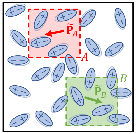
Figure 5: Fluctuations of electric polarization $\tilde{{\bf P\mit}}$ in bulk dielectric. Although there is no external electric field, the polarization continuously and randomly changes due to the thermal jiggling of polar molecules. Two arbitrary regions $A$ and $B$ are shown.

Importantly, the fluctuations in regions $A$ and $B$ are not independent, due to electrostatic interactions of polar molecules. Indeed, if we consider a single molecule, it can have any orientation with equal probability. However, when we consider two molecules, then for a given orientation of the first, the various orientations of the second will be not equally probable (with a higher probability it will orient so that the potential energy of interaction is minimized). This correlation of polarization fluctuations at different locations is conventionally characterized by the correlation function $\langle\tilde{P}_{A}\tilde{P}_{B}\rangle$, which implies, basically, averaging with respect to probabilities of various values of $\tilde{P}_{A}$ and $\tilde{P}_{B}$ [120, § 116]. To verify that this correlation function makes sense, one can consider the case when $\tilde{P}_{A}$ and $\tilde{P}_{B}$ can have arbitrary values independently. Then for any given $\tilde{P}_{A,i}$, $\tilde{P}_{B}$ can be positive and negative with the same probability and summation $\sum_{j}(\tilde{P}_{A,i}\tilde{P}_{B,j})=\tilde{\Xi}_{i}$ will be zero (here and below, repeating indices imply summation according to the Einstein notation). The correlation function in this case $\langle\tilde{P}_{A}\tilde{P}_{B}\rangle=\sum_{i}\tilde{\Xi}_{i}=0$.

In addition to the spatial correlation of fluctuations, one can analogously define temporal correlations. Moreover, correlation can be between fluctuations of different macroscopic quantities, e.g. electric polarization and displacement of heat: $\langle\tilde{P}_{A}(t)\tilde{\gamma}_{B}(t+\tau)\rangle\neq 0$ (here $\tilde{\gamma}_{B}$ defines the deviation from equilibrium along a given direction in region $B$, such as fluctuation of temperature in space [10, Eq. (4.3)] and $\tau$ is the time delay between the two fluctuations). Lars Onsager recognized the fact that due to microscopic reversibility, some specific polarization $\tilde{P}=\tilde{P}_{0}$, followed $\tau$ later by some specific heat displacement $\tilde{\gamma}=\tilde{\gamma}_{0}$, must occur just as often as the displacement $\tilde{\gamma}=\tilde{\gamma}_{0}$, followed $\tau$ later by the polarization $\tilde{P}=\tilde{P}_{0}$ [10, Eq. (4.10)]:

$$\langle\tilde{P}_{A}(t)\tilde{\gamma}_{B}(t+\tau)\rangle=\langle\tilde{P}_{A}(t+\tau)\tilde{\gamma}_{B}(t)\rangle.$$

The same equation written for fluctuations of general macroscopic quantities $\tilde{x}_{i}$ and $\tilde{x}_{k}$ read

$$\langle\tilde{x}_{i}(t)\tilde{x}_{k}(t+\tau)\rangle=\sigma\langle\tilde{x}_{i}(t+\tau)\tilde{x}_{k}(t)\rangle,$$ (24)

where $\sigma=1$ if quantities $\tilde{x}_{i}$ and $\tilde{x}_{k}$ have the same time-reversal symmetry (see Table I) and $\sigma=-1$ if they have the opposite symmetry [120, § 119]. In the frequency domain, relation (24) can be written as [120, see Eq. (122.11)]

$${x}_{i}{x}_{k}=\sigma{x}_{k}{x}_{i},$$ (25)

where definition ${x}_{i}{x}_{k}=\int_{-\infty}^{\infty}\langle\tilde{x}_{i}(t+\tau)\tilde{x}_{k}(t)\rangle{\rm e}^{-j\omega\tau}{\rm d}\tau$ was used.

Relations (24) and (25) indicate constraints on fluctuations of physical quantities in the equilibrium imposed by the microscopic time reversibility. Next, we need to determine what constraints are imposed by microscopic reversibility on stationary processes under small external perturbations. Stationary processes are processes during which the system can be considered near thermodynamic equilibrium, i.e. in quasi-equilibrium; there are no net macroscopic flows of energy) at each moment of time. In the presence of an external perturbation, a physical quantity $\tilde{x}_{i}(t)$ in addition to the fluctuations acquires some nonzero mean value $\overline{\tilde{x}}_{i}(t)$:

$$\overline{\tilde{x}}_{i}(t)=\int_{0}^{\infty}\tilde{\alpha}_{ik}(\tau)\tilde{f}_{k}(t-\tau){\rm d}\tau.$$ (26)

In this relation $\tilde{\alpha}_{ik}$ is the so-called generalized susceptibility tensor which relates the response of the system $\overline{\tilde{x}}_{i}(t)$ to the generalized forces $\tilde{f}_{k}(t)$ [120, Eq. (125.2)]. Note that integration in (26) extends from 0 to $+\infty$, rather than from $-\infty$ to $+\infty$, due to the causality principle applicable to all physical processes (see the beginning of Section II-C). One can see that one special case described by (26) is material relation (4), where the role of the generalized forces is played by the three vectorial components of the electric field and the electric displacement vector is the response function. Relation (26) is applicable to all linear causal perturbation processes.

The relation between fluctuations and perturbation processes is given by the fluctuation-dissipation theorem [121], [120, § 125]:

$${x}_{i}{x}_{k}=\frac{-j\hbar}{2}({\alpha}_{ki}^{\ast}-{\alpha}_{ik})\coth{\frac{\hbar\omega}{2k_{\rm B}T}},$$ (27)

where $k_{\rm B}$ is the Boltzmann constant, $\hbar$ is the reduced Planck constant, and $T$ is the temperature. The theorem states that thermal fluctuations of some macroscopic quantity in a system in thermal equilibrium (the left-hand side) have the same nature as the dissipation processes related to this quantity in the system in thermal quasi-equilibrium (the brackets on the right-hand side). Applied to the electric polarization, the theorem implies that the intensity of the polarization fluctuations in the material is proportional to the imaginary part of its permittivity which is responsible for dissipation of energy in the material. Thus, if there is a process accompanied by energy dissipation into heat, there should exist a reversed process which converts heat into thermal fluctuations. Other examples of such dual processes include loss in electrical resistance and Johnson noise, air resistance and Brownian motion, etc.

Substituting (27) into both sides of Eq. (25), one obtains relation

$${\alpha}_{ki}^{\ast}-{\alpha}_{ik}=\sigma({\alpha}_{ik}^{\ast}-{\alpha}_{ki}),$$ (28)

which together with the Kramers-Kronig formulae results in [120, Eq. (125.13)]

$${\alpha}_{ki}(\omega)=\sigma{\alpha}_{ik}(\omega).$$ (29)

Note that in Eqs. (28)–(29), for every combination of $i$ and $k$ indices, parameter $\sigma$ should be chosen either $+1$ when the response quantities $\tilde{x}_{i}$ and $\tilde{x}_{k}$ have the same symmetry under time-reversal or $-1$ when they have the opposite symmetry. Relations (29), stemming from microscopic reversibility conditions (24), are referred to as the Onsager reciprocal relations. They impose a fundamental restriction on the generalized susceptibility tensors of arbitrary nature. If the relations are satisfied, the system is called reciprocal. When they do not hold, it is said that the system is nonreciprocal.

Subsequently, H. Casimir pointed out that although nonreciprocal systems, i.e. systems with external time-odd bias, such as the magnetic field, are not constrained by relations (29), there is another relation which they must obey. This relation reads [12]

$${\alpha}_{ki}(\omega,{\bf H\mit}_{0})=\sigma{\alpha}_{ik}(\omega,-{\bf H\mit}_{0}).$$ (30)

Here for the sake of compactness, we denote all the bias parameters as a single time-odd parameter, the magnetic field vector ${\bf H\mit}_{0}$. Relations (30) are referred to as the Onsager-Casimir relations. They cannot be used to determine whether a system is reciprocal or nonreciprocal since they hold for either of these cases. These relations can be applied to a variety of irreversible physical processes of different nature [122]: Acoustic, electromagnetic, mechanical, thermoelectric, diffusion, etc. In what follows, we consider two examples of application of the Onsager reciprocal relations (29) to electromagnetic processes.

As the first example of a physical process subject to the Onsager reciprocal relations, we examine radiation from electromagnetic sources. Here we assume that the sources are represented by some electric current density distribution ${{\bf J\mit}}({\bf r\mit})$ with the dimensions of A/${\rm m}^{2}$ in a general non-homogeneous and anisotropic medium. The electric field radiated by the sources (in the frequency domain) is given by the volume integral equation

$${{\bf E\mit}}({\bf r\mit})=\int_{V}\bar{\bar{{G}}}({\bf r\mit},{\bf r\mit}^{\prime})\cdot{{\bf J\mit}}({\bf r\mit}^{\prime}){\rm d}V^{\prime},$$ (31)

where $\bar{\bar{{G}}}({\bf r\mit},{\bf r\mit}^{\prime})$ is dyadic Green’s function. For example, for an isotropic homogeneous medium with relative permeability ${\mu}$ it has simple form [123, p. 30]:

$$\bar{\bar{{G}}}({\bf r\mit},{\bf r\mit}^{\prime})=\bar{\bar{{G}}}({\bf r\mit}^{\prime},{\bf r\mit})=-j\omega{\mu}\mu_{0}\left[\bar{\bar{I}}+\frac{1}{k^{2}}\nabla\nabla\right]\frac{{\rm e}^{-jk|{\bf r\mit}-{\bf r\mit}^{\prime}|}}{4\pi|{\bf r\mit}-{\bf r\mit}^{\prime}|}.$$ (32)

Green’s function describes how strong is an elementary electric field ${\rm d}{{\bf E\mit}}({\bf r\mit})$ at point ${\bf r\mit}$ created by an elementary single point source ${{\bf J\mit}}({\bf r\mit}^{\prime}){\rm d}V^{\prime}$ at point ${\bf r\mit}^{\prime}$:

$${\rm d}{{\bf E\mit}}({\bf r\mit})=\bar{\bar{{G}}}({\bf r\mit},{\bf r\mit}^{\prime})\cdot{{\bf J\mit}}({\bf r\mit}^{\prime}){\rm d}V^{\prime}.$$ (33)

By integrating (33) over the overall volume of the source currents $V$, one obtains (31). Relation (33) implies the linear (the electric field is a linear function of the current density) and causal (electric field is the response function of the system depending on the current radiation in the past only) process. Taking into account macroscopic reversibility of the process (no weak interactions occur in the process) and assuming that it evolves in thermodynamic quasi-equilibrium, one can see that Green’s function satisfies all the conditions of a generalized susceptibility in (26). Let us assume now that there are no external bias fields in the system, i.e. ${\bf H\mit}_{0}=0$ (the opposite case will be considered below; see relation (44)). Applying the Onsager reciprocal relations (29) for the two infinitesimal current sources positioned at ${\bf r\mit}$ and ${\bf r\mit}^{\prime}$, one can obtain

$$\bar{\bar{{G}}}({\bf r\mit},{\bf r\mit}^{\prime})=\bar{\bar{{G}}}^{T}({\bf r\mit}^{\prime},{\bf r\mit}),$$ (34)

where $T$ denotes the transpose operator. In the derivations, the response functions $\overline{{x}}_{i}$ and $\overline{{x}}_{k}$ were replaced by ${\rm d}{{\bf E\mit}}({\bf r\mit})=\bar{\bar{{G}}}({\bf r\mit},{\bf r\mit}^{\prime})\cdot{{\bf J\mit}}({\bf r\mit}^{\prime}){\rm d}V^{\prime}$ and ${\rm d}{{\bf E\mit}}({\bf r\mit}^{\prime})=\bar{\bar{{G}}}({\bf r\mit}^{\prime},{\bf r\mit})\cdot{{\bf J\mit}}({\bf r\mit}){\rm d}V$, respectively. Note that we used the fact that parameter $\sigma$ in (30) is equal to $+1$ since all the response quantities (the components of the electric field $\tilde{E}_{x}$, $\tilde{E}_{y}$, and $\tilde{E}_{z}$) are time-even under time reversal. It can be checked that dyadic Green’s function in the form (32) satisfies the reciprocity relation (34). This fact implies that the process of radiation from electromagnetic sources in a homogeneous medium described by scalar permittivity ${\varepsilon}$ and permeability ${\mu}$ is reciprocal.

It is interesting to see what kind of symmetry on the sources and their fields is imposed by the relation for dyadic Green’s function (34). In order to do that, we consider the simplest electromagnetic system consisting of two sources ${{\bf J\mit}}_{A}$ and ${{\bf J\mit}}_{B}$ whose locations are described by vectors ${\bf r\mit}_{A}$ and ${\bf r\mit}_{B}$ (in fact ${\bf r\mit}_{A}$ and ${\bf r\mit}_{B}$ define a manifold of vectors which indicate directions to all possible point sources in $A$ and $B$), respectively. Similar considerations can be made for a system of three and more sources. Let us assume that the sources are located at different positions and have arbitrary orientations in the $xz$-plane (the current densities have only the $x$ and $z$ components), as shown in Fig. 6. Using (33), one can find the electric fields created by elementary single points belonging to $A$ and $B$ current sources:

$$\begin{array}[]{cc}\displaystyle\begin{pmatrix}{\rm d}{E}_{A,x}\\ {\rm d}{E}_{A,z}\end{pmatrix}=\begin{pmatrix}{G}_{xx}&{G}_{xz}\\ {G}_{zx}&{G}_{zz}\end{pmatrix}\cdot\begin{pmatrix}{J}_{A,x}{\rm d}V_{A}\\ {J}_{A,z}{\rm d}V_{A}\end{pmatrix},\vspace{5pt}\\ \displaystyle\begin{pmatrix}{\rm d}{E}_{B,x}\\ {\rm d}{E}_{B,z}\end{pmatrix}=\begin{pmatrix}{G}_{xx}&{G}_{xz}\\ {G}_{zx}&{G}_{zz}\end{pmatrix}\cdot\begin{pmatrix}{J}_{B,x}{\rm d}V_{B}\\ {J}_{B,z}{\rm d}V_{B}\end{pmatrix},\end{array}$$ (35)

where ${\rm d}{{\bf E\mit}}_{A}$ and ${\rm d}{{\bf E\mit}}_{B}$ correspond to the electric fields at positions ${\bf r\mit}_{B}$ and ${\bf r\mit}_{A}$ created by sources ${{\bf J\mit}}_{A}{\rm d}V_{A}$ and ${{\bf J\mit}}_{B}{\rm d}V_{B}$, respectively. System (35) comprises four equations with respect to four components of dyadic Green’s function. One can rewrite it as

$$\begin{array}[]{l}\displaystyle\begin{pmatrix}{G}_{xx}&{G}_{xz}\\ {G}_{zx}&{G}_{zz}\end{pmatrix}\vspace{5pt}\\ \displaystyle\hskip 20.0pt=\begin{pmatrix}{\rm d}{E}_{A,x}&{\rm d}{E}_{B,x}\\ {\rm d}{E}_{A,z}&{\rm d}{E}_{B,z}\end{pmatrix}\cdot\begin{pmatrix}{J}_{A,x}{\rm d}V_{A}&{J}_{B,x}{\rm d}V_{B}\\ {J}_{A,z}{\rm d}V_{A}&{J}_{B,z}{\rm d}V_{B}\end{pmatrix}^{-1}.\end{array}$$ (36)

For reciprocal systems, relation (34) requires that ${G}_{xz}={G}_{zx}$, and, therefore, from (36) it follows that

$$\begin{array}[]{ll}\displaystyle{\rm d}{E}_{B,x}{J}_{A,x}{\rm d}V_{A}+{\rm d}{E}_{B,z}{J}_{A,z}{\rm d}V_{A}\vspace{5pt}\\ \displaystyle\hskip 56.9055pt={\rm d}{E}_{A,x}{J}_{B,x}{\rm d}V_{B}+{\rm d}{E}_{A,z}{J}_{B,z}{\rm d}V_{B}.\end{array}$$ (37)

Next, one can likewise repeat the derivations (35)–(37) for two other scenarios, when the current densities have only the $y$, $z$ and only the $x$, $y$ components. Then one obtains two other equations similar to (37) but with the interchanged component indices. Summing up these two equations together with (37), we derive

$${\rm d}{{\bf E\mit}}_{B}\cdot{{\bf J\mit}}_{A}{\rm d}V_{A}={\rm d}{{\bf E\mit}}_{A}\cdot{{\bf J\mit}}_{B}{\rm d}V_{B}.$$ (38)

The integration of equation (38) over the volume occupied by the current source $A$ (over all possible ${\bf r\mit}_{A}$) for a fixed point ${\bf r\mit}_{B}$ yields

$$\int\limits_{V_{A}}{\rm d}{{\bf E\mit}}_{B}\cdot{{\bf J\mit}}_{A}{\rm d}V_{A}={{\bf E\mit}}_{A}\cdot{{\bf J\mit}}_{B}{\rm d}V_{B}.$$ (39)

Next, we integrate the last equation over the volume occupied by the current source $B$ (over all possible ${\bf r\mit}_{B}$) for a fixed point ${\bf r\mit}_{A}$:

$$\int\limits_{V_{A}}{{\bf E\mit}}_{B}\cdot{{\bf J\mit}}_{A}{\rm d}V_{A}=\int\limits_{V_{B}}{{\bf E\mit}}_{A}\cdot{{\bf J\mit}}_{B}{\rm d}V_{B}.$$ (40)

The obtained relation for two electromagnetic sources and their fields in an anisotropic non-homogeneous medium is a reciprocity condition which is called the Lorentz reciprocity relation [9]. Notably, it was discovered by H. Lorentz in 1896, long before the Onsager reciprocal relations, which we used for our derivation, were known. The relation (40) can be extended to the case of three and more sources. It is worthwhile to note that the above mentioned derivation of the Lorentz reciprocity relation does not require any prior knowledge. On contrary, the conventional derivation (shown shortly below) is based on the preceding knowledge that the Lorentz reciprocity relation relates scalar products of the corresponding electric fields and currents.

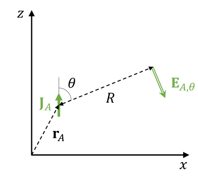
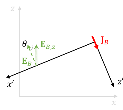
Figure 6: A system of two sources with current densities ${{\bf J\mit}}_{A}$ and ${{\bf J\mit}}_{B}$ separated by a distance $R$. (a) Radiation by source ${{\bf J\mit}}_{A}$. (b) Radiation by source ${{\bf J\mit}}_{B}$.

Likewise, one can derive similar relation which will hold for radiation in both reciprocal and nonreciprocal media. Indeed, applying the Onsager-Casimir relation (30) in our geometry with two sources at ${\bf r\mit}_{A}$ and ${\bf r\mit}_{B}$, one obtains that

$$\bar{\bar{{G}}}({\bf r\mit}_{A},{\bf r\mit}_{B},{\bf H\mit}_{0})=\bar{\bar{{G}}}^{T}({\bf r\mit}_{B},{\bf r\mit}_{A},-{\bf H\mit}_{0}).$$ (41)

Here argument $-{\bf H\mit}_{0}$ implies that the corresponding quantity should be considered in the medium with all the external bias fields reversed.

Next, let us find the final relation connecting the currents with the electric fields in a different and more general way than was given by derivations (35)–(40). Rewriting (33) for sources at ${\bf r\mit}_{A}$ and ${\bf r\mit}_{B}$, we obtain:

$$\begin{array}[]{c}\displaystyle{\rm d}{{\bf E\mit}}_{B}({\bf r\mit}_{A},{\bf H\mit}_{0})=\bar{\bar{{G}}}({\bf r\mit}_{A},{\bf r\mit}_{B},{\bf H\mit}_{0})\cdot{{\bf J\mit}}_{B}({\bf r\mit}_{B}){\rm d}V_{B},\vspace{5pt}\\ \displaystyle{\rm d}{{\bf E\mit}}_{A}({\bf r\mit}_{B},-{\bf H\mit}_{0})=\bar{\bar{{G}}}({\bf r\mit}_{B},{\bf r\mit}_{A},-{\bf H\mit}_{0})\cdot{{\bf J\mit}}_{A}({\bf r\mit}_{A}){\rm d}V_{A}.\end{array}$$ (42)

Using (41) and (42), it is easy to show that ${\rm d}{{\bf E\mit}}_{B}({\bf r\mit}_{A},{\bf H\mit}_{0})\cdot{{\bf J\mit}}_{A}({\bf r\mit}_{A}){\rm d}V_{A}$ equals

$$\begin{array}[]{ll}\displaystyle\left[\bar{\bar{{G}}}({\bf r\mit}_{A},{\bf r\mit}_{B},{\bf H\mit}_{0})\cdot{{\bf J\mit}}_{B}({\bf r\mit}_{B})\right]^{T}{{\bf J\mit}}_{A}({\bf r\mit}_{A}){\rm d}V_{A}{\rm d}V_{B}\vspace{5pt}\\ \displaystyle={{\bf J\mit}}_{B}^{T}({\bf r\mit}_{B})\bar{\bar{{G}}}^{T}({\bf r\mit}_{A},{\bf r\mit}_{B},{\bf H\mit}_{0}){{\bf J\mit}}_{A}({\bf r\mit}_{A}){\rm d}V_{A}{\rm d}V_{B}\vspace{5pt}\\ \displaystyle={{\bf J\mit}}_{B}({\bf r\mit}_{B})\cdot\left[\bar{\bar{{G}}}({\bf r\mit}_{B},{\bf r\mit}_{A},-{\bf H\mit}_{0}){{\bf J\mit}}_{A}({\bf r\mit}_{A}){\rm d}V_{A}\right]{\rm d}V_{B}\vspace{5pt}\\ \displaystyle={\rm d}{{\bf E\mit}}_{A}({\bf r\mit}_{B},-{\bf H\mit}_{0})\cdot{{\bf J\mit}}_{B}({\bf r\mit}_{B}){\rm d}V_{B}.\end{array}$$ (43)

Integrating this equality like it was done in (39)–(40), we obtain

$$\int\limits_{V_{A}}{{\bf E\mit}}_{B}({\bf H\mit}_{0})\cdot{{\bf J\mit}}_{A}{\rm d}V_{A}=\int\limits_{V_{B}}{{\bf E\mit}}_{A}(-{\bf H\mit}_{0})\cdot{{\bf J\mit}}_{B}{\rm d}V_{B}.$$ (44)

This relation can be referred to as Onsager-Casimir theorem which is applied to both reciprocal and nonreciprocal linear time-invariant (LTI) systems. Naturally, for reciprocal media (with ${\bf H\mit}_{0}=0$) relation (44) simplifies to the Lorentz reciprocity relation (40).

Next, let us verify that relation (40) is in fact valid for two dipole sources in a homogeneous isotropic medium illustrated in Fig. 6. The sources have infinitesimal thickness and equal lengths $l$. Without loss of generality, we assume that the sources are located far from one another at a distance $R\gg\lambda$. First, we measure the radiation from source $A$, located at $\mathbf{r}_{\rm A}$ and oriented along $z$. The $\theta$-component (in the spherical coordinate system with the center at ${\bf r\mit}_{A}$) of the electric field ${{\bf E\mit}}_{A}$ generated at point $\mathbf{r}_{\rm B}=\mathbf{r}_{\rm A}+\mathbf{R}$ can be written as [124, Eq. (1.72a)]:

$${E}_{A,\theta}=j\omega{\mu}\mu_{0}\frac{{I}_{A}l}{4\pi}\frac{{\rm e}^{-jkR}}{R}\sin\theta,$$ (45)

where ${I}_{A}$ is the electric current flowing through dipole $A$. In the second scenario, we measure the radiation from source $B$ which is oriented along the $\theta$-direction with respect to the initial $xyz$ basis for simplifying the calculations. The electric field in the position of dipole $A$ can be written as:

$${E}_{B}=j\omega{\mu}\mu_{0}\frac{{I}_{B}l}{4\pi}\frac{{\rm e}^{-jkR}}{R}.$$ (46)

The projection of this field to the $z$-axis (the direction in which dipole $A$ is oriented) is ${E}_{B,z}={E}_{B}\sin\theta$. Finally, substituting ${E}_{A,\theta}$ and ${E}_{B,z}$ in (31) and applying scalar product, we get:

$${E}_{B,z}{I}_{A}l={E}_{A,\theta}{I}_{B}l,$$ (47)

which is obviously an equality.

As the second example of a physical process subject to the Onsager reciprocal relations, we consider polarization of a general bianisotropic dipolar scatterer. Incident electric (or magnetic) field induces electric and magnetic dipole moments [116, 125]. The derivation below are based on [116, § 3.3.1]. The electric ${{\bf p\mit}}$ and magnetic ${{\bf m\mit}}$ dipoles induced in a bianisotropic scatterer are related to the incident fields through electric $\bar{\bar{{\alpha}}}_{\rm ee}$, magnetic $\bar{\bar{{\alpha}}}_{\rm mm}$, magnetoelectric $\bar{\bar{{\alpha}}}_{\rm me}$, and electromagnetic $\bar{\bar{{\alpha}}}_{\rm em}$ polarizability tensors:

$$\begin{pmatrix}{{\bf p\mit}}\\ {{\bf m\mit}}\end{pmatrix}=\begin{pmatrix}\bar{\bar{{\alpha}}}_{\rm ee}&\bar{\bar{{\alpha}}}_{\rm em}\\ \bar{\bar{{\alpha}}}_{\rm me}&\bar{\bar{{\alpha}}}_{\rm mm}\end{pmatrix}\cdot\begin{pmatrix}{{\bf E\mit}}\\ {{\bf H\mit}}\end{pmatrix}.$$ (48)

This equations can be written using the six-vector notations as

$$\overline{{p}}_{i}(\omega)={A}_{ik}(\omega)\,{e}_{k}(\omega),$$ (49)

where $\overline{{p}}_{i}$ is a vector including six components of the electric and magnetic dipole moments, ${e}_{k}$ includes, likewise, components of the electric and magnetic fields, and ${A}_{ik}$ is a $6\times 6$ tensor consisting of all the polarizability components. Equation (49) is analogous to the frequency-domain form of equation (26). Polarizability tensor ${A}_{ik}$ satisfies all the conditions of a generalized susceptibility, and, therefore, one can apply the Onsager reciprocal relations (29) and obtain ${A}_{ki}=\sigma{A}_{ik}$ for reciprocal bianisotropic scatterers. As it was mentioned earlier, for every combination of $i$ and $k$, parameter $\sigma$ should be chosen equal either $+1$ if $\tilde{p}_{i}$ and $\tilde{p}_{k}$ have the same symmetry under time reversal (when both of them are components of $\tilde{{\bf p\mit}}$ or $\tilde{{\bf m\mit}}$) or $-1$ in the opposite case (when one of them is component of $\tilde{{\bf p\mit}}$ and another is component of $\tilde{{\bf m\mit}}$). Thus, the Onsager reciprocal relations for polarization of a bianisotropic scatterer read

$$\bar{\bar{{\alpha}}}_{\rm ee}=\bar{\bar{{\alpha}}}_{\rm ee}^{T},\quad\bar{\bar{{\alpha}}}_{\rm mm}=\bar{\bar{{\alpha}}}_{\rm mm}^{T},\quad\bar{\bar{{\alpha}}}_{\rm me}=-\bar{\bar{{\alpha}}}_{\rm em}^{T}.$$ (50)

These relations can be used in order to determine whether a scatterer with given polarizability tensors is reciprocal or nonreciprocal. The Onsager-Casimir constraints (30), applicable for both reciprocal and nonreciprocal scatterers, result in

$$\begin{array}[]{ll}\displaystyle\bar{\bar{{\alpha}}}_{\rm ee}({\bf H\mit}_{0})=\bar{\bar{{\alpha}}}_{\rm ee}^{T}(-{\bf H\mit}_{0}),\quad\bar{\bar{{\alpha}}}_{\rm mm}({\bf H\mit}_{0})=\bar{\bar{{\alpha}}}_{\rm mm}^{T}(-{\bf H\mit}_{0}),\vspace{5pt}\\ \displaystyle\hskip 56.9055pt\bar{\bar{{\alpha}}}_{\rm me}({\bf H\mit}_{0})=-\bar{\bar{{\alpha}}}_{\rm em}^{T}(-{\bf H\mit}_{0}).\end{array}$$ (51)

Similarly to derivations (48)–(51), one can apply the Onsager reciprocal relations to bulk polarization of bianisotropic materials. The reader is referred to works [126],[127, Eq. (4)],[116, § 3.3.1] for detailed derivations.

IV-B The Lorentz lemma and reciprocity theorem

The Lorentz reciprocity theorem (or reciprocity relation) is formulated for a pair of sources with current densities ${{\bf J\mit}}_{A}$ and ${{\bf J\mit}}_{B}$ which create fields ${{\bf E\mit}}_{A}$ and ${{\bf E\mit}}_{B}$ [9],[128, § 5.5],[107, § 3.6.2] (see illustration in Fig. 7).

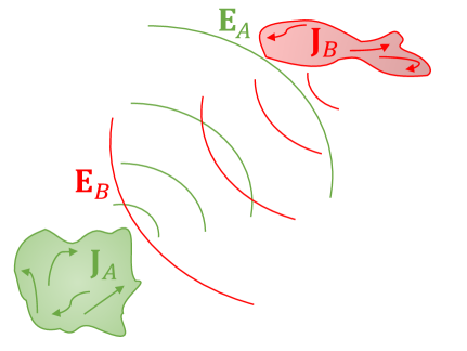
Figure 7: Electromagnetic interaction between a pair of sources with the current densities ${{\bf J\mit}}_{A}$ and ${{\bf J\mit}}_{B}$.

The derivation of this theorem for the general case of a linear homogeneous medium was described in the previous section. Here, we formulate this theorem for the special case of bianisotropic media and discuss its implications on the material tensors. Before we proceed to the theorem statement, let us declare an auxiliary quantity called reaction and introduced in [129]. The reaction of field ${{\bf E\mit}}_{B}$ on a source with current density ${{\bf J\mit}}_{A}$ is defined by the following volume integral in the frequency domain:

$$\langle A,B\rangle=\int\limits_{V_{A}}{{\bf J\mit}}_{A}\cdot{{\bf E\mit}}_{B}{\rm d}V_{A},$$ (52)

where the volume $V_{A}$ contains the source $A$, and ${\rm d}V_{A}$ is the volume element. Likewise, the reaction of field ${{\bf E\mit}}_{A}$ on the source with current density ${{\bf J\mit}}_{B}$ is given by

$$\langle B,A\rangle=\int\limits_{V_{B}}{{\bf J\mit}}_{B}\cdot{{\bf E\mit}}_{A}{\rm d}V_{B}.$$ (53)

Note that we met this reaction quantity in (40). The reaction should be distinguished from the rate of work done on a given charge distribution, despite the fact that these quantities have the same units. The latter one describes the dot product of the electric field and the current ${{\bf J\mit}}_{\rm ind}$ that it induces in the material, i.e. $\int_{V}{{\bf J\mit}}_{\rm ind}\cdot{{\bf E\mit}}{\rm d}V$.

Using the assumed linearity of the system, we can express the fields created by sources by corresponding Green’s functions. We stress that these Green’s functions are not just simple free-space Green’s functions, they take into account possibly very complicated topology of inhomogeneous bianisotropic media. Substituting the electric field from (31) in (52) and (53), we obtain

$$\langle A,B\rangle=\int_{V_{A}}\int_{V_{B}}\mathbf{{J}}_{A}\cdot\bar{\bar{{G}}}({\bf r\mit}_{A},{\bf r\mit}_{B})\cdot\mathbf{{J}}_{B}\,{\rm d}V_{B}{\rm d}V_{A},$$ (54)

$$\begin{array}[]{c}\displaystyle\langle B,A\rangle=\int_{V_{B}}\int_{V_{A}}\mathbf{{J}}_{B}\cdot\bar{\bar{{G}}}({\bf r\mit}_{B},{\bf r\mit}_{A})\cdot\mathbf{{J}}_{A}\,{\rm d}V_{A}{\rm d}V_{B}\vspace{2mm}\\ \displaystyle=\int_{V_{B}}\int_{V_{A}}\mathbf{{J}}_{A}\cdot\bar{\bar{{G}}}^{T}({\bf r\mit}_{B},{\bf r\mit}_{A})\cdot\mathbf{{J}}_{B}\,{\rm d}V_{A}{\rm d}V_{B},\end{array}$$ (55)

where we replaced scalar $\mathbf{{J}}_{B}\cdot\bar{\bar{{G}}}\cdot\mathbf{{J}}_{A}$ by its transpose $(\mathbf{{J}}_{B}\cdot\bar{\bar{{G}}}\cdot\mathbf{{J}}_{A})^{T}$ and used tensor identity $(\mathbf{{J}}_{B}\cdot\bar{\bar{{G}}}\cdot\mathbf{{J}}_{A})^{T}=\mathbf{{J}}_{A}\cdot\bar{\bar{{G}}}^{T}\cdot\mathbf{{J}}_{B}$. If the system satisfies the assumption made in the derivation of the Onsager symmetry relation (29), Green’s function is symmetric, i.e. $\bar{\bar{{G}}}({\bf r\mit}_{A},{\bf r\mit}_{B})=\bar{\bar{{G}}}^{T}({\bf r\mit}_{B},{\bf r\mit}_{A})$, which implies that the two reactions are equal:

$$\langle A,B\rangle-\langle B,A\rangle=\int\limits_{V_{A}}{{\bf J\mit}}_{A}\cdot{{\bf E\mit}}_{B}{\rm d}V_{A}-\int\limits_{V_{B}}{{\bf J\mit}}_{B}\cdot{{\bf E\mit}}_{A}{\rm d}V_{B}=0.$$ (56)

Equation (56) represents the Lorentz reciprocity theorem (or relation) in the frequency domain. It states that in reciprocal systems, the reaction of field ${{\bf E\mit}}_{A}$ on a source with current density ${{\bf J\mit}}_{B}$ should be the same as that of field ${{\bf E\mit}}_{B}$ on a source with ${{\bf J\mit}}_{A}$. In other words, interactions between any pair of electromagnetic sources are reciprocal. Relation (56) can be considered as the definition of reciprocal electromagnetic systems. This formulation, in fact, does not imply time reversibility $t\rightarrow-t$ of electromagnetic processes in the medium. Instead, it is based on the notion of restricted time reversal and just emulates time reversibility by interchanging the locations of the sources and the field probe.

Let us find the restriction on material properties dictated by the Lorentz reciprocity, i.e. conditions on material parameters which determine whether a given material is reciprocal or not. First, we can write the Maxwell equations in the frequency domain applied to each of the two volumetric sources:

$$\begin{array}[]{c}\displaystyle\nabla\times{{\bf E\mit}}_{A}=-j\omega\mathbf{{{\bf B\mit}}_{A}},\quad\nabla\times{\bf H\mit}_{A}=j\omega\mathbf{{{\bf D\mit}}_{A}}+{{\bf J\mit}}_{A},\vspace{1mm}\\ \displaystyle\nabla\times{{\bf E\mit}}_{B}=-j\omega\mathbf{{{\bf B\mit}}_{B}},\quad\nabla\times{\bf H\mit}_{B}=j\omega\mathbf{{{\bf D\mit}}_{B}}+{{\bf J\mit}}_{B}.\end{array}$$ (57)

Using (57), we obtain the following relation for the difference of reactions $\langle A,B\rangle-\langle B,A\rangle$:

$$\begin{array}[]{l}\displaystyle\int\limits_{V}{{\bf J\mit}}_{A}\cdot{{\bf E\mit}}_{B}\,{\rm d}V-\int\limits_{V}{{\bf J\mit}}_{B}\cdot{{\bf E\mit}}_{A}\,{\rm d}V\vspace{2mm}\\ \displaystyle=\oint\limits_{S}\left({{\bf E\mit}}_{A}\times{{\bf H\mit}}_{B}-{{\bf E\mit}}_{B}\times{{\bf H\mit}}_{A}\right)\cdot d{\bf S\vspace{2mm}}\mit\\ \displaystyle-j\omega\int\limits_{V}\left({{\bf E\mit}}_{B}\cdot{{\bf D\mit}}_{A}-{{\bf E\mit}}_{A}\cdot{{\bf D\mit}}_{B}+{{\bf H\mit}}_{A}\cdot{{\bf B\mit}}_{B}-{{\bf H\mit}}_{B}\cdot{{\bf B\mit}}_{A}\right){\rm d}V,\end{array}$$ (58)

which represents the so-called Lorentz lemma. Note that lemma (58) is just a mathematically derived equation from the Maxwell equations, and it does not imply any reciprocity conditions, being applicable for both reciprocal and nonreciprocal time-invariant systems. Here, we have used the Gauss theorem and an identity from vector calculus ${\bf F\mit}\cdot(\nabla\times{\bf G\mit})=\nabla\cdot({\bf G\mit}\times{\bf F\mit})+{\bf G\mit}\cdot(\nabla\times{\bf F\mit})$. Volume $V$ and its closed surface area $S$ include both sources $A$ and $B$.

We stress that the only condition for the validity of the Lorentz lemma (not Lorentz reciprocity theorem) is that both sets of fields satisfy Maxwell’s equations and that the involved integrals exist. The two sets of sources can act in two different media, which can have arbitrary electromagnetic properties including nonlinear. Below we consider the Lorentz lemma for three different scenarios: Reciprocal and nonreciprocal time-invariant media, as well as time-varying media.

IV-B1 Reciprocal time-invariant media

For monochromatic fields (restricting the generality to sources at the same frequency in linear time-invariant media), the Lorentz lemma (58) together with the Lorentz reciprocity relation (56) result in

$$\begin{array}[]{l}\displaystyle 0=\oint\limits_{S}\left({{\bf E\mit}}_{A}\times{{\bf H\mit}}_{B}-{{\bf E\mit}}_{B}\times{{\bf H\mit}}_{A}\right)\cdot{\rm d}{\bf S\vspace{2mm}}\mit\\ \displaystyle-j\omega\int\limits_{V}\left({{\bf E\mit}}_{B}\cdot{{\bf D\mit}}_{A}-{{\bf E\mit}}_{A}\cdot{{\bf D\mit}}_{B}+{{\bf H\mit}}_{A}\cdot{{\bf B\mit}}_{B}-{{\bf H\mit}}_{B}\cdot{{\bf B\mit}}_{A}\right){\rm d}V.\end{array}$$ (59)

The surface integral in (59) vanishes since the surface of integration can be always extended to infinity from the sources where the electric and magnetic fields are related through ${{\bf H\mit}}_{A,B}={\bf n\mit}\times{{\bf E\mit}}_{A,B}/{\eta}$ and ${\bf n\mit}\cdot{{\bf E\mit}}_{A,B}=0$, where ${\eta}$ is the impedance of the surrounding medium and ${\bf n\mit}$ is the unit normal vector to the integration surface pointing outwards. Indeed, the expression in the surface integral becomes zero since ${{\bf E\mit}}_{A}\times{{\bf H\mit}}_{B}-{{\bf E\mit}}_{B}\times{{\bf H\mit}}_{A}={\bf n\mit}({{\bf E\mit}}_{A}\cdot{{\bf E\mit}}_{B})-{\bf n\mit}({{\bf E\mit}}_{B}\cdot{{\bf E\mit}}_{A})=0$. This argument, resulting into vanishing of the surface integral, can be applied only for the case when the medium is homogeneous and isotropic at the considered boundary. Nevertheless, it is possible to proof that the surface integral tends to zero even in the case of a general medium. This proof is conventionally made based on the so-called limiting absorption principle [130, 131]. One can assume a tiny absorption everywhere. In this case, the fields will exponentially decay, and hence the surface integral vanishes as the boundary goes to infinity. Next, one can take the limit of the absorption going to zero. Thus, this principle yields vanishing surface integral even in the lossless case.

Assuming that the integration space is filled with a nonuniform bianisotropic medium (general linear medium whose parameters arbitrarily vary in space) [128, 116] with macroscopic material relations

$$\begin{array}[]{l}\displaystyle\mathbf{{{\bf D\mit}}}_{A,B}=\bar{\bar{{\varepsilon}}}(\mathbf{r},\omega)\cdot\mathbf{{E}}_{A,B}+\bar{\bar{{\xi}}}(\mathbf{r},\omega)\cdot\mathbf{{H}}_{A,B},\vspace{1mm}\\ \displaystyle\mathbf{{{\bf B\mit}}}_{A,B}=\bar{\bar{{\zeta}}}(\mathbf{r},\omega)\cdot\mathbf{{E}}_{A,B}+\bar{\bar{{\mu}}}(\mathbf{r},\omega)\cdot\mathbf{{H}}_{A,B},\end{array}$$ (60)

equation (59) yields (here, $\bar{\bar{{\xi}}}$ and $\bar{\bar{{\zeta}}}$ are the bianisotropy parameters describing effects of weak spatial dispersion [132])

$$\begin{array}[]{l}\displaystyle-j\omega\int\limits_{V}\Big{\{}\mathbf{{E}}_{B}\cdot\left[\bar{\bar{{\varepsilon}}}-\bar{\bar{{\varepsilon}}}^{T}\right]\cdot\mathbf{{E}}_{A}+\mathbf{{H}}_{A}\cdot\left[\bar{\bar{{\mu}}}-\bar{\bar{{\mu}}}^{T}\right]\cdot\mathbf{{H}}_{B}\vspace{2mm}\\ \displaystyle+\mathbf{{E}}_{B}\cdot\left[\bar{\bar{{\xi}}}+\bar{\bar{{\zeta}}}^{T}\right]\cdot\mathbf{{H}}_{A}-\mathbf{{H}}_{B}\cdot\left[\bar{\bar{{\zeta}}}+\bar{\bar{{\xi}}}^{T}\right]\cdot\mathbf{{E}}_{A}\Big{\}}{\rm d}V=0.\end{array}$$ (61)

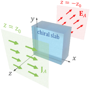
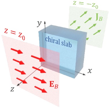
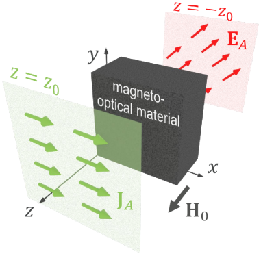
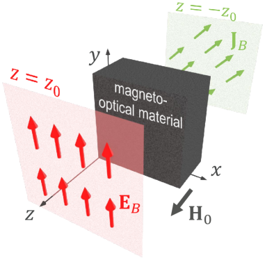
Figure 8: Application of the Lorentz reciprocity theorem for (a–b) a chiral slab and (c–d) a slab of magneto-optical material. The theorem holds only for the reciprocal chiral slab.

To obtain this equation, we have used the same tensor identity as in (55). Since this equation is satisfied for arbitrary fields ${{\bf E\mit}}_{\rm A,B}$ and ${{\bf H\mit}}_{\rm A,B}$, the expressions in the square brackets in (61) must be equal to zero, which results in

$$\bar{\bar{{\varepsilon}}}=\bar{\bar{{\varepsilon}}}^{T},\quad\bar{\bar{{\mu}}}=\bar{\bar{{\mu}}}^{T},\quad\bar{\bar{{\xi}}}=-\bar{\bar{{\zeta}}}^{T}.$$ (62)

Equations (62) are the Onsager reciprocal relations applied on material parameters of general bianisotropic reciprocal media. Materials for which these conditions are not satisfied are nonreciprocal. Note that these relations are similar to those for polarizabilities of a single bianisotropic scatterer given by (50). In fact, relations (62) can be alternatively achieved using derivations similar to (48)–(50). It should be mentioned that not all time-reversible (in microscopic sense) systems are reciprocal, while all reciprocal systems are time-reversible. On the other hand, as was shown in [117, p. 697], the restricted time reversibility of a medium has the same conditions on material tensors as in (62). Therefore, reciprocity and restricted time-reversal symmetry apply in the same way to different materials (see the bottom rows of the table in Fig. 4).

Let us consider the applicability of the Lorentz reciprocity theorem for two simple examples of isotropic materials. In the first example, we consider a bianisotropic chiral slab whose structural units (molecules or meta-atoms) have broken mirror symmetry. We position an infinite current sheet with ${{\bf J\mit}}_{A}$ in front of the slab at $z=z_{0}$ and probe the electric field ${{\bf E\mit}}_{A}$ which was radiated by the sheet and passed through the slab at the plane $z=-z_{0}$, as shown in Fig. 8. The wave passed through the chiral slab experienced polarization rotation by an azimuthal angle $\phi=+45^{\circ}$. When we interchange the plane of the source with the observation plane (see Fig. 8), the wave radiated by the sheet with current density ${{\bf J\mit}}_{B}$ (tilted at $45^{\circ}$) is transmitted through the chiral slab with opposite polarization rotation at an angle $\phi=-45^{\circ}$. Now, it is clear that the surface integral of the reaction $\int_{S}{{\bf J\mit}}_{A}\cdot{{\bf E\mit}}_{B}{\rm d}S$ is equal to $\int_{S}{{\bf J\mit}}_{B}\cdot{{\bf E\mit}}_{A}{\rm d}S$, which means that the chiral slab is reciprocal.

In the second example, let us consider a slab of magneto-optical material biased by a static magnetic field ${\bf H\mit}_{0}$. Such slab rotates polarization of a wave passed through it at the same angle $+45^{\circ}$ regardless the propagation direction. Therefore, repeating the same thought experiment shown in Figs. 8 and 8, one can observe that $\int_{S}{{\bf J\mit}}_{A}\cdot{{\bf E\mit}}_{B}{\rm d}S=0$ (${{\bf J\mit}}_{A}$ and ${{\bf E\mit}}_{B}$ are orthogonal), while $\int_{S}{{\bf J\mit}}_{B}\cdot{{\bf E\mit}}_{A}{\rm d}S\neq 0$. This result confirms that biased magneto-optical materials are nonreciprocal.

Thus, in the simplified formulation, reciprocity of a system implies that under interchanging the positions of the source and the observation point, the detected field does not change (regardless of losses in the system). This statement follows from the Lorentz lemma (56), assuming ${{\bf J\mit}}_{A}={{\bf J\mit}}_{B}$. Graphically such principle is depicted in Fig. 4 in cells A.3, B.3, and C.3. Observing Fig. 4, one can conclude that pointwise reciprocity of a linear time-invariant system implies that it is locally time-reversible in the restricted sense, and vice versa.

IV-B2 Nonreciprocal time-invariant media

It should be mentioned that the Onsager relations can be extended to nonreciprocal materials [126, 133]. By reversing time of the whole system (globally, including time of the external sources), we obtain the time-reversed process.

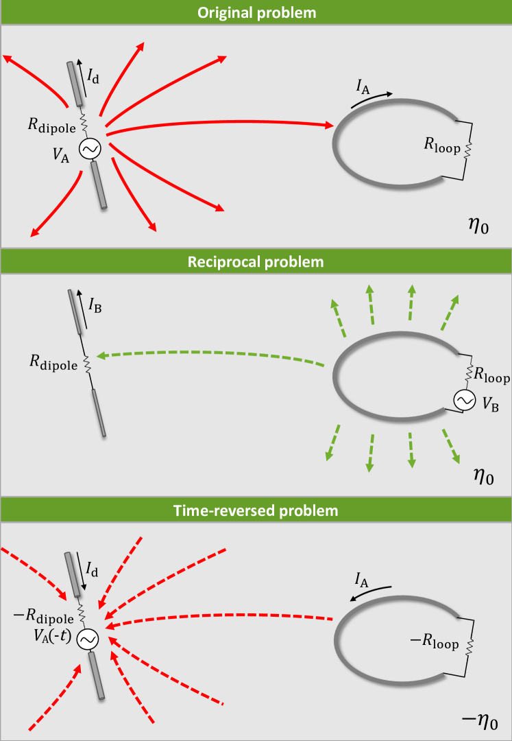
Figure 9: Reciprocity and time-reversibility applied to antenna problems. Original problem is presented in the top figure.

Let us assume that the field ${{\bf E\mit}}_{B}$ generated by the source $B$ is calculated in the same material but with reversed bias fields ${\bf H\mit}_{0}$ (to emulate global time reversibility). In this reversed material, the material relations (60) for the case of excitation by source with ${{\bf J\mit}}_{B}$ can be written as

$$\begin{array}[]{l}\displaystyle\mathbf{{{\bf D\mit}}}_{B}=\bar{\bar{{\varepsilon}}}(\mathbf{r},\omega,-\mathbf{H}_{0})\cdot\mathbf{{E}}_{B}+\bar{\bar{{\xi}}}(\mathbf{r},\omega,-\mathbf{H}_{0})\cdot\mathbf{{H}}_{B},\vspace{1mm}\\ \displaystyle\mathbf{{{\bf B\mit}}}_{B}=\bar{\bar{{\zeta}}}(\mathbf{r},\omega,-\mathbf{H}_{0})\cdot\mathbf{{E}}_{B}+\bar{\bar{{\mu}}}(\mathbf{r},\omega,-\mathbf{H}_{0})\cdot\mathbf{{H}}_{B}.\end{array}$$ (63)

Substituting the material relations to (59), one can obtain

$$\begin{split}-j\omega&\int_{V}\Big{\{}\mathbf{{E}}_{B}\cdot\left[\bar{\bar{{\varepsilon}}}(\mathbf{H}_{0})-\bar{\bar{{\varepsilon}}}^{T}(-\mathbf{H}_{0})\right]\cdot\mathbf{{E}}_{A}\\ &\qquad-\mathbf{{H}}_{A}\cdot\left[\bar{\bar{{\mu}}}^{T}(\mathbf{H}_{0})-\bar{\bar{{\mu}}}(-\mathbf{H}_{0})\right]\cdot\mathbf{{H}}_{B}\\ &\qquad+\mathbf{{E}}_{B}\cdot\left[\bar{\bar{{\xi}}}(\mathbf{H}_{0})+\bar{\bar{{\zeta}}}^{T}(-\mathbf{H}_{0})\right]\cdot\mathbf{{H}}_{A}\\ &\qquad-\mathbf{{H}}_{B}\cdot\left[\bar{\bar{{\zeta}}}(\mathbf{H}_{0})+\bar{\bar{{\xi}}}^{T}(-\mathbf{H}_{0})\right]\cdot\mathbf{{E}}_{A}\Big{\}}{\rm d}V=0,\end{split}$$ (64)

from where the Onsager-Casimir relations for material parameters read

$$\begin{array}[]{c}\displaystyle\bar{\bar{{\varepsilon}}}(\mathbf{H}_{0})=\bar{\bar{{\varepsilon}}}^{T}(-\mathbf{H}_{0}),\qquad\bar{\bar{{\mu}}}(\mathbf{H}_{0})=\bar{\bar{{\mu}}}^{T}(-\mathbf{H}_{0}),\vspace{1mm}\\ \displaystyle\bar{\bar{{\xi}}}(\mathbf{H}_{0})=-\bar{\bar{{\zeta}}}^{T}(-\mathbf{H}_{0}).\end{array}$$ (65)

These conditions on material parameters can be applied to both reciprocal and nonreciprocal media. For the former case, the conditions simplify to (62). Note that these relations are similar to those for polarizabilities of a single bianisotropic scatterer given by (51) and can be alternatively derived likewise.

A classical application of reciprocity in time-invariant media is to antenna problems. Let us assume the scenario shown in Fig. 9 (top picture), where two antennas are placed in free space. In particular, we will consider a dipole antenna excited by a voltage source $V_{\rm A}$ and a receiving loop. The current excited in the dipole produces radiated fields which propagate in the background medium and induce a current in the loop antenna, denoted as $I_{\rm A}$. In the reciprocal scenario, we consider the dipole as a receiving antenna and the loop becomes the transmitting antenna excited by the voltage source $V_{\rm B}$. In this case, the current excited in the loop emits propagating fields that induce a current $I_{\rm B}$ in the dipole (see the middle picture). The Lorentz reciprocity theorem presented in Eq. (56) can be simplified as $V_{\rm A}I_{\rm B}=V_{\rm B}I_{\rm A}$ for this particular example. It is interesting to notice that the fields in the reciprocal scenario are not the time-reversed copy of the fields in the original example. As it is shown in Fig. 9 (bottom picture), in the time-reversal scenario, both loop and dipole resistors become active elements modeled by the negative resistors and the voltage source becomes a sink. Even more interesting, the impedance of the background medium will also become negative modeling energy deliver from infinity by the host medium. The negative resistors excite currents that produce exactly a time-reversed copy of the field excited in the original example. Under these considerations, the time-reversal scenario seems to be physically unrealistic. To understand the relation between the reciprocity theorem and the time-reversibility of Maxwell equations, one must consider that in both original and reciprocal scenarios the interaction between receiving and transmitting antennas is produced by “direct” rays that emanate from one antenna and induce a current in the second antenna. These rays are identical in the reciprocal and time-reversed scenario and linking the reciprocal scenario with the time-reversal problem.

IV-B3 Time-varying media

Let us rewrite Maxwell’s equations for two systems. In the original system, the time argument is $t$, while in the time-reversed and shifted by $\tau$ seconds system, the argument is $\tau-t$. Thus, we have

$$\begin{split}&\nabla\times\tilde{{\bf E\mit}}(t)=-{\partial\over\partial t}\tilde{{\bf B\mit}}(t),\cr&\nabla\times\tilde{{\bf H\mit}}(t)=\tilde{{\bf J\mit}}(t)+{\partial\over\partial t}\tilde{{\bf D\mit}}(t),\cr&\nabla\times\tilde{{\bf E\mit}}(\tau-t)={\partial\over\partial t}\tilde{{\bf B\mit}}(\tau-t),\cr&\nabla\times\tilde{{\bf H\mit}}(\tau-t)=\tilde{{\bf J\mit}}(\tau-t)-{\partial\over\partial t}\tilde{{\bf D\mit}}(\tau-t).\end{split}$$ (66)

Using the following identity: $\nabla\cdot({\bf C\mit}\times{\bf D\mit})={\bf D\mit}\cdot(\nabla\times{\bf C\mit})-{\bf C\mit}\cdot(\nabla\times{\bf D\mit})$, and employing the above expressions based on Maxwell’s equations, we can readily conclude that

$$\begin{split}&\nabla\cdot\Big{(}\tilde{{\bf E\mit}}_{A}(\tau-t)\times\tilde{{\bf H\mit}}_{B}(t)-\tilde{{\bf E\mit}}_{B}(t)\times\tilde{{\bf H\mit}}_{A}(\tau-t)\Big{)}=\cr&\tilde{{\bf H\mit}}_{A}(\tau-t)\cdot{\partial\over\partial t}\tilde{{\bf B\mit}}_{B}(t)+\tilde{{\bf H\mit}}_{B}(t)\cdot{\partial\over\partial t}\tilde{{\bf B\mit}}_{A}(\tau-t)\cr&-\tilde{{\bf E\mit}}_{A}(\tau-t)\cdot{\partial\over\partial t}\tilde{{\bf D\mit}}_{B}(t)-\tilde{{\bf E\mit}}_{B}(t)\cdot{\partial\over\partial t}\tilde{{\bf D\mit}}_{A}(\tau-t)\cr&-\tilde{{\bf E\mit}}_{A}(\tau-t)\cdot\tilde{{\bf J\mit}}_{B}(t)+\tilde{{\bf E\mit}}_{B}(t)\cdot\tilde{{\bf J\mit}}_{A}(\tau-t).\end{split}$$ (67)

Here, for simplicity we assume that there are only electric current sources. If we integrate over a volume $V$ which contains both sources and over time $t$, we express the most general form of the Lorentz lemma (compare to (58)).

For a time-invariant medium, two different forms of the Lorentz reciprocity can be introduced: Convolution-type and correlation-type reciprocity [134, 135]. Probably the most studied type is the convolution type which is given by

$$\begin{split}\int_{-\infty}^{+\infty}{\rm d}t\int_{V}&\tilde{{\bf J\mit}}_{A}(\tau-t)\cdot\tilde{{\bf E\mit}}_{B}(t){\rm d}V=\cr&\int_{-\infty}^{+\infty}{\rm d}t\int_{V}\tilde{{\bf J\mit}}_{B}(t)\cdot\tilde{{\bf E\mit}}_{A}(\tau-t){\rm d}V.\end{split}$$ (68)

This is a general definition in the time domain which is exactly equivalent to the Lorentz reciprocity relation in the frequency domain (see Eq. (56)). This is due to the fact that in Eq. (68), as mentioned in the above, the convolution operation on the electric current density and the electric field is applied. Let us develop Eq. (67). To do that, we can also include the material relations corresponding to a time-invariant medium. Remember that in the time domain, such relations are given by

$$\begin{split}&\mathbf{\tilde{D}}(t)=\int_{0}^{\infty}\bar{\bar{\tilde{\varepsilon}}}(\tau)\cdot\mathbf{\tilde{E}}(t-\tau){\rm d}\tau+\int_{0}^{\infty}\bar{\bar{\tilde{\xi}}}(\tau)\cdot\mathbf{\tilde{H}}(t-\tau){\rm d}\tau,\cr&\mathbf{\tilde{B}}(t)=\int_{0}^{\infty}\bar{\bar{\tilde{\zeta}}}(\tau)\cdot\mathbf{\tilde{E}}(t-\tau){\rm d}\tau+\int_{0}^{\infty}\bar{\bar{\tilde{\mu}}}(\tau)\cdot\mathbf{\tilde{H}}(t-\tau){\rm d}\tau.\end{split}$$ (69)

Now, by considering the Lorentz lemma (67), employing the convolution-type reciprocity (68), and substituting the material relations (69), after doing some algebraic manipulations, we obtain the following expressions in time domain:

$$\bar{\bar{\tilde{\varepsilon}}}(t)=\bar{\bar{\tilde{\varepsilon}}}^{T}(t),\,\,\,\,\,\,\bar{\bar{\tilde{\mu}}}(t)=\bar{\bar{\tilde{\mu}}}^{T}(t),\,\,\,\,\,\,\bar{\bar{\tilde{\xi}}}(t)=-\bar{\bar{\tilde{\zeta}}}^{T}(t).$$ (70)

These relations are equivalent to those for frequency-domain material tensors given by Eqs. (62).

Regarding a linear time-varying medium, whose macroscopic material parameters change in time, developing Eq. (67) needs that we replace the material relations which take into account the general integral transform, and this is not a simple task. According to that general form, the electric and magnetic flux densities are expressed as

$$\begin{split}&\mathbf{\tilde{D}}(t)=\int_{0}^{\infty}\hat{\tilde{\varepsilon}}(\tau,t)\cdot\mathbf{\tilde{E}}(t-\tau){\rm d}\tau+\int_{0}^{\infty}\hat{\tilde{\xi}}(\tau,t)\cdot\mathbf{\tilde{H}}(t-\tau){\rm d}\tau,\cr&\mathbf{\tilde{B}}(t)=\int_{0}^{\infty}\hat{\tilde{\zeta}}(\tau,t)\cdot\mathbf{\tilde{E}}(t-\tau){\rm d}\tau+\int_{0}^{\infty}\hat{\tilde{\mu}}(\tau,t)\cdot\mathbf{\tilde{H}}(t-\tau){\rm d}\tau,\end{split}$$ (71)

where $\hat{\tilde{\varepsilon}}(\tau,t)$, $\hat{\tilde{\mu}}(\tau,t)$, $\hat{\tilde{\xi}}(\tau,t)$, and $\hat{\tilde{\zeta}}(\tau,t)$ are operators depending on each moment of time $t$ [136]. In this case, the response at any moment of time is associated strongly with these operators expressed at that moment. However, it is not the case for a time-invariant medium, in which Eq. (71) is simplified to Eq. (69). This equation involves the conventional convolution integrals, while Eq. (71) takes into account the general integral transform and as a consequence, developing the Lorentz lemma is not easy due to the dependency on $t$.

It should be mentioned that the Lorentz reciprocity relation (68) can be applied to linear time-varying systems since all the requirements for the Onsager reciprocal relations (linearity, causality, microscopic reversibility, and thermodynamic quasi-equilibrium) are satisfied for such systems.

IV-C Reciprocity applied to scattering parameters

In many scenarios of solving an electromagnetic problem, it is not necessary to obtain exact wave solution at all points in space. Sometimes it is sufficient to determine the fields or voltages and currents only at specific boundaries (terminals). In this case, we model a set of various electromagnetic components of arbitrary complexity as a “black box”, to be exact, an electrical network. When an external electromagnetic signal or wave interact with this network, we need to study only what output it produces for a given input, without solving the fields inside the network. An example of an electrical network is a transmitting antenna. Fed with an AC signal at its terminals, an antenna radiates electromagnetic waves in surrounding space. To improve radiation efficiency, one needs to decrease the parasitic reflections at the antenna terminals due to the impedance mismatch by adding a matching circuit. Full-wave solution of this problem (using the Maxwell equations) would be a resource-demanding task. Instead, we model the antenna as a “black box” with one input channel through the cable (a one-port network) and the matching circuit as a two-port network. Subsequently, we determine the required properties of the matching circuit (its response to input) and design it using basic circuit elements.

There is plenty of different parameters for description of electrical networks [2, Ch. 4],[137, Ch. 3]. Here, we will discuss only the scattering parameters (S-parameters) since they relate the input (the generalized forces) to the output signals or waves (response functions). As a consequence, we can directly apply to them the Onsager reciprocal relations. Other parameters, such as impedance, admittance, and transmission (ABCD) matrices, relate quantities which include both input and output signals. Reciprocity relations for such parameters can be derived from those of the scattering parameters (all these parameters can be expressed in terms of one another [2, p. 192]). According to the conventional notations of $N$-port networks, the scattering coefficients $S_{ij}$ relate the normalized amplitudes of an incoming and an outgoing signals. Scattering coefficients give information about the reflected or transmitted power and the phase shift produced by the system. In the matrix form, the scattering parameters can be expressed as

$$\left[\begin{array}[]{cc}b_{1}\\ b_{2}\\ \vdots\\ b_{\rm N}\end{array}\right]=\left[\begin{array}[]{cccc}S_{11}&S_{12}&\cdots&S_{1N}\\ S_{21}&&&\vdots\\ \vdots&&&\\ S_{N1}&\cdots&&S_{NN}\end{array}\right]\left[\begin{array}[]{cc}a_{1}\\ a_{2}\\ \vdots\\ a_{N}\end{array}\right],$$ (72)

where $a_{i}$ and $b_{i}$ with $i=1,2,...N$ represent the incoming and outgoing signals, respectively (see Fig. 10). With this definition, the tangential components of the fields in each port can be expressed as:

$$\mathbf{{E}}_{t,i}=(a_{i}+b_{i})\mathbf{{e}}_{i},\qquad\mathbf{{H}}_{t,i}=(a_{i}-b_{i})\mathbf{{h}}_{i}$$ (73)

with $i=1..N$ denoting the port number. If scattering matrix is applied for circuits, the fields in (73) should be replaced by voltages and currents. The vectors $\mathbf{{e}}_{i}$ and $\mathbf{{h}}_{i}$ represent the electric and magnetic modal fields in port $i$. All the ports must be linearly independent, i.e. the fields should satisfy the orthogonality condition $\iint{{\bf e\mit}}_{i}\cdot{{\bf e\mit}}_{j}{\rm d}S=\delta_{ij}$ [137, p. 5], where the integration is extended over the cross section of the port and $\delta_{ij}$ denotes the Kronecker delta.

Although usually scattering parameters are used for circuits in microwave engineering, they can be successfully applied for plane-wave propagation through different media. Consider normal incidence of a wave of a given polarization on an interface of two materials. This system can be characterized by two ports corresponding to the two sides of the interface. Now assume that the polarization of incident waves can be partially rotated by $90^{\circ}$. In this case, it is convenient to model the interface by a four-port network: Two ports for the waves with original polarization and two other for the waves with rotated polarization. The ports are independent since the two polarizations are orthogonal. The scattering matrix concept can be extended to diffraction gratings with multiple orders [138]. They provide a simple way to determine the power balance between different diffraction orders, the reciprocity conditions, etc.

As it was mentioned, the scattering parameters satisfy the conditions of the generalized susceptibilities (26) and, additionally, all the requirements imposed on the Onsager reciprocal relations (29). Since all the response functions in (72) have the same time-reversal symmetry (e.g., electric fields, magnetic fields, or currents), parameter $\sigma$ in (29) must be taken $+1$ for all $i,k$ indices. As a result, the reciprocity condition for scattering matrix is given by

$$\overline{\overline{S}}=\overline{\overline{S}}^{T}.$$ (74)

In the general case, all systems (both reciprocal and nonreciprocal) must satisfy the Onsager-Casimir relation (30) which is written for S-parameters as

$$\overline{\overline{S}}({\bf H\mit}_{0})=\overline{\overline{S}}^{T}(-{\bf H\mit}_{0}).$$ (75)

Interestingly, condition (74) determines only overal reciprocity of a network. A network can consist of multiple nonreciprocal components which compensate each other (pointwise nonreciprocity), while appear as reciprocal when probed at its ports. An example is a combination of two ferrite slabs magnetized in the opposite directions. Considering the system as a black box, one can only conclude that it is overal reciprocal.

Next, we will discuss how the characteristic of the system can be fathomed from the properties of the scattering matrix and give classical examples of reciprocal and nonreciprocal devices.

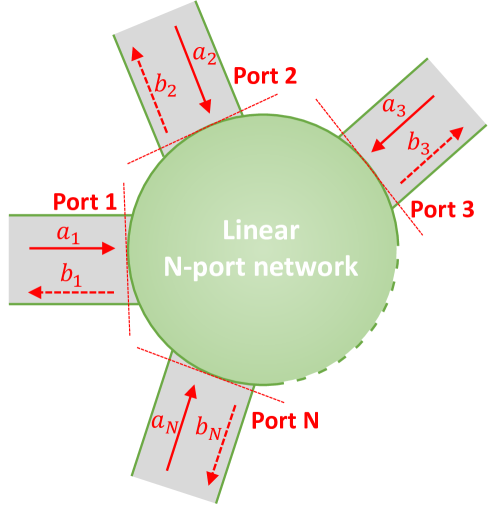
Figure 10: Schematic representation of a linear time-invariant $N$-port network and the scattering coefficients.

Reciprocal lossless systems: The scattering matrix is symmetric for reciprocal systems and unitary for lossless systems [2, § 4.3]. The latter condition is expressed as $(\overline{\overline{S}}^{\ast})^{T}\cdot\overline{\overline{S}}=\overline{\overline{I}}$. For example, if we consider a simultaneously lossless and reciprocal 2-port system, the scattering matrix can be expressed as

$$\begin{array}[]{c}\left[\begin{array}[]{cc}S_{11}&S_{12}\\ S_{21}&S_{22}\end{array}\right]=\left[\begin{array}[]{cc}{\rm e}^{j\theta}\sin{\beta}&{\rm e}^{j\phi}\cos{\beta}\\ {\rm e}^{j\phi}\cos{\beta}&{\rm e}^{j\zeta}\sin{\beta}\end{array}\right],\end{array}$$ (76)

where $\beta\in[0;\pi/2]$ and the arguments satisfy the condition $2\phi-\theta-\zeta=\pi+2\pi m$ with $m$ being integer. An example of such a system is an isotropic non-dissipative dielectric slab (two interfaces define two ports), where we find symmetric transmissions and reflection. When multiple orthogonal modes are supported by each port (as in the case of plane waves with orthogonal polarizations), one can replace scalar elements in (76) by tensors $\overline{\overline{S}}_{11}$, $\overline{\overline{S}}_{22}$, $\overline{\overline{S}}_{12}$, and $\overline{\overline{S}}_{21}$. In this case, the reciprocal conditions are defined as $\overline{\overline{S}}_{11}=\overline{\overline{S}}_{11}^{T}$, $\overline{\overline{S}}_{22}=\overline{\overline{S}}_{22}^{T}$, $\overline{\overline{S}}_{12}=\overline{\overline{S}}_{21}^{T}$.

Nonreciprocal and lossless systems: It is evident that lossless and reciprocal systems provide a reduced number of degrees of freedom for the design. There are applications where it is necessary to break the strong condition imposed by reciprocity. For example, one can think of phase shifters with different phase shifts depending on the direction. A canonical example of such devices is the gyrator, a two-port network that introduces asymmetric phases in transmission with $\pi$ difference between them

$$\begin{array}[]{c}\overline{\overline{S}}_{\rm gyrator}=\left[\begin{array}[]{cc}0&1\\ -1&0\end{array}\right].\end{array}$$ (77)

A gyrator is considered as a fundamental non-reciprocal element that in combination with four other reciprocal elements, that is a resistor, capacitor, inductor, and ideal transformer, completes the set of building blocks needed for constructing an arbitrarily complex linear passive network [139].

For example, another nonreciprocal and lossless device is a circulator, a three-port device where the signal can flow between ports 1$\rightarrow$2$\rightarrow$3, but not in the opposite direction. The scattering matrix of an ideal circulator can be expressed as

$$\begin{array}[]{c}\overline{\overline{S}}_{\rm circulator}=\left[\begin{array}[]{ccc}0&0&1\\ 1&0&0\\ 0&1&0\end{array}\right].\end{array}$$ (78)

A three-port circulator can be constructed using the basic nonreciprocal building block, the gyrator, and two quaterwave transmission lines.

These scattering matrices that characterize these two examples are unitary, meaning that they are lossless systems.

Nonreciprocal and lossy systems: Finally, there are devices whose matrices are not symmetric nor unitary. One of the most important devices fulfilling these properties is the isolator:

$$\begin{array}[]{c}\overline{\overline{S}}_{\rm isolator}=\left[\begin{array}[]{cc}0&0\\ 1&0\end{array}\right].\end{array}$$ (79)

This two-port device allows transmission in one direction, but both transmission or reflection are forbidden in the opposite direction. Importantly, lossless isolators cannot exist: A two-port network described by the above scattering matrix is matched at both ports, meaning that the wave falling on the isolated port cannot be reflected back and must be absorbed inside the isolator.

Scattering parameters provide a most useful tool for the analysis of linear time-invariant systems that has been used in the microwave engineering since the 1960´s. This formulation has been extended to time-variant systems [66],[90, § XIV], although these generalized parameters have restricted use. In the most general case, each terminal of the network is characterized by $M$-modes and $P$-frequencies. Considering that the system has $N$ different terminals, the characterization will be done using $N\times M\times P$ ports. For linear time-variant systems, the expression for each scattering parameter will be similar to the LTI case, $S_{ij}=b_{i}/a_{j}$. Lorentz reciprocity for time-variant systems was considered in [66].

IV-D Different routes for breaking reciprocity

Here, we delve into the necessary physical conditions that warrant reciprocity in a system, as well as the possible ways to break it. In the derivation of the Onsager reciprocal relations presented in Section IV-A, the following physical assumptions were used:

1. time-reversal symmetry of microscopic equations,

2. linear response,

3. causal response,

4. thermodynamic quasi-equilibrium.

The last condition should be discussed separately. All the previous formulations were supported by the assumption of thermodynamic quasi-equilibrium or, in other words, assumption that the system is in a stable and stationary state reached after interactions with its surroundings for enough long time (so-called linear or Onsager region [140]). In this state, there are no net macroscopic flows of thermal energy. Particularly, in electromagnetic theory, this regime is achieved when the perturbations produced by the applied fields are slow enough to ensure that the particles equilibrate to the surrounding particles.

In order to achieve nonreciprocity in a system, at least one of the mentioned conditions must be made invalid (however, it is not a sufficient condition). Thus, we can list several possible routes towards breaking reciprocity. The first condition of time-reversal symmetry of microscopic equations can be violated by introducing to the system a time-odd external force/parameter ${\bf H\mit}_{0}$. In this case, relation (29) does not hold anymore ${\alpha}_{ki}(\omega,{\bf H\mit}_{0})\neq\sigma{\alpha}_{ik}(\omega,{\bf H\mit}_{0})$, and the system may exhibit nonreciprocal response. Possible time-odd external parameters include but not limited to:

• external magnetic fields, e.g., applied to plasma or ferrite (see detailed discussion in Section V-A),

• exchange interaction force, e.g. in antiferromagnets,

• linear velocity using linearly moving structures or linear space-time modulation (see detailed discussion in Section VII),

• angular velocity (rotating objects or space-time modulation emulating rotation).

A separate discussion on the external time-odd parameters for breaking reciprocity will be given in Section V-C. Analogous routes towards electromagnetic nonreciprocity were reported in review paper [90, Table I].

The second condition of linear response can be naturally broken using nonlinear systems. However, as it will be discussed in Section VI, the nonlinearity route for breaking reciprocity is not universal and has its own limitations [44, 53]. The causality assumption does not apply to active systems, meaning that reciprocity can be broken in systems comprising amplifiers or parametric amplifiers [54, 141, 142].

The use of systems far from equilibrium also appears possible for achieving nonreciprocity. It is known that the fluctuation–dissipation theorem is violated in non-equilibrium glassy systems (systems which slowly approach their equilibrium state) [143]. In such systems the Onsager reciprocal relations do not necessarily hold.

V Nonreciprocity in linear time-invariant media

In this section, phenomenological description of two nonreciprocal effects, namely Faraday rotation and Kerr ellipticity, is given. We list LTI materials in which these effects can occur. Furthermore, we introduce a general classification of nonreciprocal LTI media based on their time- and space-reversal symmetries.

V-A Nonreciprocal effects using LTI materials

Probably, the first known nonreciprocal effect dates back to the discovery by Faraday, made in 1845. He observed polarization rotation of linearly polarized light propagating through a rod of lead borate glass placed in an external static magnetic field [144]. By changing the direction of the magnetic field or the direction of the incident light beam, the sense of rotation is reversed. This property makes the Faraday rotation effect distinct from natural optical rotation in chiral materials. Linearly polarized light encounters double polarization rotation upon travelling through magnetically biased material forth and back. Whereas, the effect of natural optical rotation (chirality) vanishes in this case.

Let us present a phenomenological description of the Faraday effect in the framework of classical electrodynamics. Such description provides an intuitive route for understanding physics of the effect. However, its microscopic origin is based on the spin-orbit interaction (Zeeman effect) and relativistic effects [1, Ch. 5].

Consider a free electron located in the lattice of positively charged ions of a magneto-optical material. An incident light applies an external force on the electron, resulting in its displacement from the center of the atomic orbital. Here, we neglect the Lorentz force imposed on the electron by the alternating magnetic field since it is typically much weaker than that by the electric field (see Ref. [145] where the Lorentz force contribution is taken into account). Nevertheless, if the considered material is biased by a strong static magnetic field, the Lorentz force acting on the electron by this field must be included in the analysis. Let us assume the incident light with right circular polarization (RCP) propagating in the material biased by an external magnetic flux density $B_{0}{\bf z\mit}_{0}$ (with the direction towards the source of light). It will cause the electron circulation in the polarization $x_{0}y_{0}$ plane, as depicted in Fig. 11. Note that the rotation of the electron occurs in the same direction as the rotation of the incident electric field vector, despite the fact that the electron has negative electric charge. It is not the instanteneous electric field that affects the electron motion direction, but its dynamics. Here, we use the definition of the handedness sense as in electrical engineering literature [2, p. 24], which is opposite to that in the optics literature [1, § 2.4].

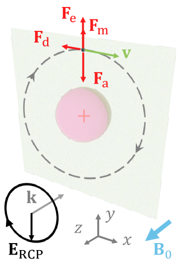
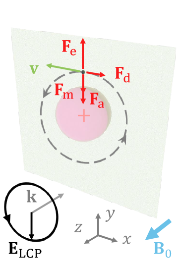
Figure 11: Phenomenological description of circular birefringence of a magneto-optical material in external magnetic field. The illustration depicts a free electron in the vicinity of positively charged ion. Due to the oppositely directed Lorentz force, incident right and left polarized light cause electron’s circulation at different orbit (cyclotron) radii, resulting in different refractive indices of the material.

There are four forces acting on the electron in this configuration: The attractive Coulomb force pointing towards the center of the atomic orbital $\tilde{{\bf F\mit}}_{\rm a}=-k_{\rm a}\tilde{{\bf r\mit}}$, the friction force $\tilde{{\bf F\mit}}_{\rm d}=-\Gamma{\rm d}\tilde{{\bf r\mit}}/{\rm d}t$ due to energy dissipation and directed opposite to electron’s velocity, the force applied by the alternating electric field $\tilde{{\bf F\mit}}_{\rm e}=e\tilde{{\bf E\mit}}_{\rm i}$, and the Lorentz force acting on the circulating electron by the static magnetic field $\tilde{{\bf F\mit}}_{\rm m}=eB_{0}{\rm d}\tilde{{\bf r\mit}}/{\rm d}t\times{\bf z\mit}_{0}$. Here $k_{\rm a}$ is the effective stiffness coefficient, $\Gamma$ is the dissipation factor, $e$ is the elementary charge, and $\tilde{{\bf r\mit}}$ is the electron’s position vector. The same electron under illumination by incident light with left circular polarization (LCP) will circulate in the opposite direction and, therefore, will experience the oppositely directed Lorentz force, as shown in Fig. 11. Thus, the total force acting on the electron towards the atomic orbital is different for the cases of light excitation with different circular polarizations. This results in different effective cyclotron radii of the electron orbit and, subsequently, in different microscopic polarizabilities of the ion-electron pair and macroscopic refractive indices. Therefore, incident linearly polarized light (combination of right and left circularly polarized components) after propagating through the magnetized material acquires rotation of the polarization plane. Quantitative description of the mentioned effect can be made based on the Lorentzian model for the electron written in the form of Newton’s law of motion:

$$m\frac{{\rm d}^{2}\tilde{{\bf r\mit}}}{{\rm d}t^{2}}=-k_{\rm a}\tilde{{\bf r\mit}}-\Gamma\frac{{\rm d}\tilde{{\bf r\mit}}}{{\rm d}t}+e\tilde{{\bf E\mit}}_{\rm i}+eB_{0}\frac{{\rm d}\tilde{{\bf r\mit}}}{{\rm d}t}\times{\bf z\mit}_{0},$$ (80)

where $m$ is the electon mass. By performing the direct Fourier transform to (80), one obtains the equation of motion in the frequency domain [146, 147]:

$$(m\omega_{0}^{2}-m\omega^{2}+j\omega\Gamma)\,{{\bf r\mit}}=e{{\bf E\mit}}_{\rm i}+jeB_{0}\omega{{\bf r\mit}}\times{\bf z\mit}_{0},$$ (81)

where $\omega$ is the angular frequency of electron motion, ${{\bf r\mit}}$ and ${{\bf E\mit}}_{\rm i}$ are the functions of $\omega$, $\omega_{0}=\sqrt{k_{\rm a}/m}$ is the material dependent constant with the dimensions of angular frequency. Writing the incident electric field in the form ${{\bf E\mit}}_{\rm i}={E}_{{\rm i}x}{\bf x\mit}_{0}+{E}_{{\rm i}y}{\bf y\mit}_{0}$ and the position vector as ${{\bf r\mit}}=x{{\bf x\mit}}_{0}+y{{\bf y\mit}}_{0}$, one obtains the following system of equations with respect to coordinates of the electron ${x}(\omega)$ and ${y}(\omega)$:

$$\begin{array}[]{c}\displaystyle(m\omega_{0}^{2}-m\omega^{2}+j\omega\Gamma){x}(\omega)-j\omega eB_{0}{y}(\omega)=e{E}_{{\rm i}x},\vspace{1mm}\\ \displaystyle(m\omega_{0}^{2}-m\omega^{2}+j\omega\Gamma){y}(\omega)+j\omega eB_{0}{x}(\omega)=e{E}_{{\rm i}y}.\end{array}$$ (82)

Assuming circular polarization of incident light ${E}_{{\rm i}y}=\pm j{E}_{{\rm i}x}={E}_{\rm i}/\sqrt{2}$ (upper and bottom signs stand for right and left circular polarizations, respectively), we conclude that electron’s motion is indeed circular ${y}(\omega)=\pm j{x}(\omega)={r}(\omega)/\sqrt{2}$ and the electric polarizability of the ion-electron pair ${\alpha}_{\rm\frac{RCP}{LCP}}(\omega)=e{r}(\omega)/{E}_{\rm i}(\omega)/\varepsilon_{0}$ is given by

$${\alpha}_{\rm\frac{RCP}{LCP}}(\omega)=\frac{e^{2}/\varepsilon_{0}}{(m\omega_{0}^{2}-m\omega^{2}+j\omega\Gamma)\pm e\omega B_{0}}.$$ (83)

The macroscopic refractive indices of the magnetized magneto-optical material for RCP and LCP read

$${n}_{\rm\frac{RCP}{LCP}}(\omega)=\sqrt{1+N_{\rm e}{\alpha}_{\rm\frac{RCP}{LCP}}(\omega)}={n}^{\prime}_{\rm\frac{RCP}{LCP}}(\omega)-j{\kappa}_{\rm\frac{RCP}{LCP}}(\omega),$$ (84)

where $N_{\rm e}$ is the free electron concentration, ${n}^{\prime}$ and ${\kappa}$ are the real part of refractive index and extinction coefficients. The Faraday rotation angle for linearly polarized light is readily calculated [146, 147] using

$$\theta_{\rm F}(\omega)=\frac{\omega L}{2c}[{n}^{\prime}_{\rm RCP}(\omega)-{n}^{\prime}_{\rm LCP}(\omega)],$$ (85)

where $L$ is the thickness of the magneto-optical slab and $c$ stands for speed of light in vacuum. The Faraday rotation angle is counted in such a way that it is related to the direction of ${\bf B\mit}_{0}$ by the right hand rule. When $B_{0}=0$, the Faraday rotation angle becomes zero.

It is easy to demonstrate that the Faraday rotation angle flips sign for the opposite light propagation direction. Indeed, for the opposite illumination, direction of the magnetic static field with respect to the light wavevector reverses. This means that refractive indices for the opposite illumination ${n}_{\rm\frac{RCP}{LCP}}^{\rm op}={n}_{\rm\frac{LCP}{RCP}}$ and the sense of rotation is flipped, i.e. $\theta_{\rm F}^{\rm op}=-\theta_{\rm F}$. This conclusion is in full agreement with Figs. 8 and 8 and, as it was shown in Section IV-B, such material response corresponds to a nonreciprocal effect. The Faraday ellipticity which determines how elliptical linearly polarized light becomes after passing through the magneto-optical material is expressed as[146]

$$\tan\psi_{\rm F}(\omega)=\tanh\left(\frac{\omega L}{2c}[{\kappa}_{\rm RCP}(\omega)-{\kappa}_{\rm LCP}(\omega)]\right).$$ (86)

The ellipticity angle $\psi_{\rm F}$ is defined as the angle between the major axis of the ellipse and the diagonal of the rectangle that circumscribes the ellipse [1, § 2.4].

Next, solving Eqs. (82) separately for linearly polarized light beams along the $x$- and $y$-directions, one can determine the diagonal ${\varepsilon}_{xx}={\varepsilon}_{yy}={\varepsilon}_{\rm s}$ and off-diagonal ${\varepsilon}_{xy}=-{\varepsilon}_{yx}=j{\varepsilon}_{\rm a}$ components of permittivity tensor given by (15):

$$\begin{array}[]{l}\displaystyle{\varepsilon}_{xx}={\varepsilon}_{yy}=1+N_{\rm e}e\frac{{x}(\omega)}{\varepsilon_{0}{E}_{{\rm i}x}(\omega)}\vspace{1mm}\\ \displaystyle\qquad\qquad=1+\Delta(m\omega_{0}^{2}-m\omega^{2}+j\omega\Gamma),\vspace{1mm}\\ \displaystyle{\varepsilon}_{yx}=-{\varepsilon}_{xy}=N_{\rm e}e\frac{{y}(\omega)}{\varepsilon_{0}{E}_{{\rm i}x}(\omega)}=-j\Delta\,\omega eB_{0},\vspace{1mm}\\ \displaystyle\Delta=\frac{N_{\rm e}e^{2}/\varepsilon_{0}}{(m\omega_{0}^{2}-m\omega^{2}+j\omega\Gamma)^{2}-(\omega eB_{0})^{2}}.\end{array}$$ (87)

As is seen from (87), the off-diagonal component of the permittivity tensor is proportional to the static magnetic flux density $B_{0}$ (in the limit of small field, directly proportional). It should be noted that in the accurate quantum mechanical description, permittivity tensor depends on the material magnetization $\mu_{0}M$, rather than magnetic flux density $B_{0}$ [148, § 5.6.5],[149, § 5.2.2]. If dissipation is negligible ($\Gamma=0$), one can observe that the diagonal permittivity components become purely real, while the off-diagonal ones become purely imaginary. One can also see from (87) that the resonance of the cyclotron orbiting occurs at the frequency where the real part in the denominator of parameter $\Delta$ equals zero. This frequency is usually written as $\omega_{\rm c}=eB_{0}/m_{\rm eff}$ [20, p. 571], where $m_{\rm eff}$ is the effective mass of the electron which takes into account the interaction with the ion. Since in the majority of natural materials the cyclotron frequency $\omega_{\rm c}$ is relatively low (of the order of 10-1000 GHz for typical magnetic flux density $B_{0}\sim 1$ T), in the optical range the magneto-optical effects are weak. Likewise, ferromagnetic properties of materials expressed by the antisymmetric part of the permeability tensor are weak in the optical region, since the Larmor resonance of the electron spin $\omega_{\rm L}=eB_{0}/m$ (precession of the spin angular momentum) is located in the microwave range [2, p. 454].

By analogy with polarization rotation (conversion in general lossy case) of transmitted linearly polarized light through a sample of a magneto-optical material, one should also expect polarization conversion for light reflected from such material. Such an effect is nonreciprocal, as will be proved below, and is called magneto-optical Kerr effect [150]. Depending on the mutual orientation of the magnetization direction of the material and the plane of incidence, three basic configurations of the effect are distinguished: Polar, longitudinal, and transversal. Here, we consider only the former one, i.e. polar magneto-optical Kerr effect. A normally incident light beam is linearly polarized along the $x$-axis, and the external static magnetic flux density $B_{0}{\bf z\mit}_{0}$ is along the $+z$-direction (antiparallel to the incident light direction). It is convenient to decompose the linearly polarized incident beam into two beams with left and right circular polarization, that is ${E}_{\rm i}{\bf x\mit}_{0}={{\bf E\mit}}_{\rm RCP}+{{\bf E\mit}}_{\rm LCP}=({\bf x\mit}_{0}+j{\bf y\mit}_{0}){E}_{\rm i}/2+({\bf x\mit}_{0}-j{\bf y\mit}_{0}){E}_{\rm i}/2$. Next, using the Fresnel formula for reflection coefficient, one can find the reflected field from the magneto-optical material:

$${{\bf E\mit}}_{\rm r}=\frac{1-{n}_{\rm RCP}}{1+{n}_{\rm RCP}}\frac{{E}_{\rm i}}{2}({\bf x\mit}_{0}+j{\bf y\mit}_{0})+\frac{1-{n}_{\rm LCP}}{1+{n}_{\rm LCP}}\frac{{E}_{\rm i}}{2}({\bf x\mit}_{0}-j{\bf y\mit}_{0}).$$ (88)

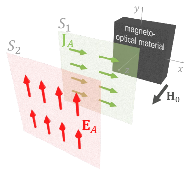
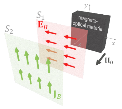
Figure 12: Application of the Lorentz reciprocity theorem for the magneto-optical Kerr effect. A biased slab of magneto-optical material reflects with additional polarization rotation an incident plane wave generated by current source (a) ${{\bf J\mit}}_{A}$ and (b) ${{\bf J\mit}}_{B}$. The theorem does not hold since $\int_{S_{1}}{{\bf J\mit}}_{A}\cdot{{\bf E\mit}}_{B}{\rm d}S\neq\int_{S_{2}}{{\bf J\mit}}_{B}\cdot{{\bf E\mit}}_{A}{\rm d}S$. The illustrations do not depict the $x$-component of ${{\bf E\mit}}_{A}$ and $y$-component of ${{\bf E\mit}}_{B}$ (incident and reflected co-polarized electric fields) since their contributions to the surface integrals are zero. The two planes $S_{1}$ and $S_{2}$ were separated by one-wavelength distance for visual clarity.

Due to the magnetization by $B_{0}$, the reflected light acquired orthogonal polarization component along the $y$-direction. The ratio

$$\frac{{E}_{{\rm r}y}}{{E}_{{\rm r}x}}=j\frac{{n}_{\rm RCP}-{n}_{\rm LCP}}{{n}_{\rm RCP}{n}_{\rm LCP}-1}$$ (89)

describes the Kerr rotation (real component of the ratio) and Kerr ellipticity (imaginary component) [146]. It can be shown using (83), (84), and (87) that 

$${n}_{\rm\frac{RCP}{LCP}}=\sqrt{{\varepsilon}_{xx}\mp j{\varepsilon}_{yx}}.$$ (90)

Note that in the lossless case both ${\varepsilon}_{xx}$ and $j{\varepsilon}_{yx}$ are purely real quantities. Since typically in natural magneto-optical materials the off-diagonal permittivity component is very small for realistic values of the bias field ($|{\varepsilon}_{yx}|\ll|{\varepsilon}_{xx}|$), we can rewrite (89) using (90) as

$$\frac{{E}_{{\rm r}y}}{{E}_{{\rm r}x}}=\frac{{\varepsilon}_{yx}}{\sqrt{{\varepsilon}_{xx}}({\varepsilon}_{xx}-1)}.$$ (91)

One can observe from (87) that for lossless magneto-optical materials ratio ${E}_{{\rm r}y}/{E}_{{\rm r}x}$ is purely imaginary, meaning that the reflected light has elliptical polarization. The axial ratio is proportional to the strength of the static magnetic field.

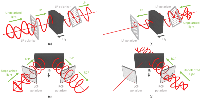
Figure 13: Electromagnetic isolation based on (a–b) Faraday effect and (c–d) magneto-optical Kerr effect. The first scenario requires presence of dissipation losses in the system, while the second scenario can be achieved in lossless systems.

In order to demonstrate that magneto-optical Kerr effect is a manifestation of nonreciprocity, we need to find the reflected light for the case when the incident light is polarized along the $y$-direction. Carrying out analogous manipulations, we obtain for this scenario the axial ratio given by

$$\frac{{E}_{{\rm r}x}}{{E}_{{\rm r}y}}=\frac{-{\varepsilon}_{yx}}{\sqrt{{\varepsilon}_{xx}}({\varepsilon}_{xx}-1)},$$ (92)

which is precisely negative of (91). In other words, some part (dictated by the right-hand side of (91)) of linearly $x$-polarized light is reflected in the $y$-polarization. However, when the incident light is $y$-polarized the same part of it is reflected in the $x$-polarization but with an additional phase flip of $180^{\circ}$ (reciprocal response would imply no phase change). Figures 12 and 12 illustrate this effect (note that for clarity the figures do not depict the incident and reflected co-polarized electric fields, as explained in the caption). Using the Lorentz reciprocity theorem (56), we conclude that $\int_{S_{1}}{{\bf J\mit}}_{A}\cdot{{\bf E\mit}}_{B}{\rm d}S\neq\int_{S_{2}}{{\bf J\mit}}_{B}\cdot{{\bf E\mit}}_{A}{\rm d}S$, and the polar magneto-optical Kerr effect is nonreciprocal.

Thus, due to the Faraday and Kerr effects, light interacting with magnetized medium acquires polarization rotation. An important question is whether the opposite effects can exist, meaning that external light interacting with a medium leads to its magnetization. Indeed, such phenomena were theoretically predicted and are called inverse Faraday [136, eq. (36a)],[151] and inverse Kerr [152] effects. Their phenomenological description, analogous to the one in the present section, can be found, e.g. in [153, 154]. The first experimental observation of the inverse Faraday effect was reported in [155]. The magnetization is induced by a circularly polarized optical pump of high energy (the circular polarization of light beam generates a solenoid trajectories of the electrons which in turn result in net magnetic moments). Therefore, this scheme can be exploited to obtain conventional Faraday polarization rotation of a probe signal without external magnetic field using only responsive optical pumping. Both these inverse effects are used for ultrafast (sub-picosecond) control of a medium magnetization for modern magnetic storage systems requiring very large operation rates [156].

Faraday and Kerr magneto-optical effects are not the only phenomena of nonreciprocal nature occuring in LTI materials. When a magnetic field is applied to a vapour or liquid through which light is passing perpendicularly to the field, magnetic linear birefringence takes place, resulting in so-called Cotton-Mouton [157] or Voigt effect [158]. This effect is typically very weak, depending quadratically on magnetization.

It should be mentioned that at microwaves, the magneto-optical effects are generally stronger than that at higher frequencies. The reason lies in the fact that microwaves are “slow enough” to excite resonant precession of electron’s magnetic moments (spin) in ferromagnetic materials. In contrast to optical frequencies, nonreciprocity in magneto-optical materials at microwaves is manifested by the off-diagonal components of the permeability tensor [159]. Due to the duality of permittivity and permeability, the Faraday and Kerr effects can be observed also at microwaves [160].

V-B Applications of nonreciprocal effects and examples of LTI nonreciprocal materials

Nonreciprocal effects in magneto-optical materials have found many important industrial applications (see a review in [1, Secs. 13,14]). First of all, the Faraday effect enables control of polarization and amplitude of the transmitted light beam. This functionality is important for optical switches [161] and light modulators [162] where fast electronic control is required. The latter is achieved via modulation of the electric current in the external electromagnet. Likewise, electronically tunable light deflection is possible using magnetic films with stripe domain structure which behave as a diffraction grating [163]. Another interesting application is related to magneto-optical drives and requires ferromagnetic materials [164]. The digital information is read from these drives based on the polar Kerr effect, discussed in the previous section. Nevertheless, after the success of the technology of magneto-optical drives in the 80-s and 90-s, it was completely surpassed by hard disk and solid-state drives.

Probably, the most eminent application of Faraday and Kerr effects is for electromagnetic isolators [165] and circulators [166]. One-way propagation based on Faraday effect is conventionally achieved in the configuration shown in Fig. 13(a) where additional two linear polarizers are used from both sides of the magneto-optical material slab. The polarizers are rotated at $45^{\circ}$ with respect to one another, and the magneto-optical slab rotates polarization of the incident light by the same angle. Thus, for illumination from the left, half of the unpolarized light is transmitted through both polarizers and the slab (see Fig. 13(a)). On the contrary, light incident from the right side does not pass through the second polarizer being reflected (see Fig. 13(b)). Importantly, in order to achieve perfect isolation effect, either polarizers or the material slab must possess certain level of dissipation losses (otherwise, isolation in the system would violate the second law of thermodynamics). Alternatively, such dissipation can be mimicked by introducing additional channel to the system, e.g. by reflecting the light from the second polarizer in Fig. 13(b) towards the direction different from the isolator symmetry axis (in principle, it can be done by tilting the second polarizer).

Material
and Ref.	Frequency range / Wavelength range	Verdet constant, $V_{\rm c}$ $[{\rm rad}/({\rm T}\cdot{\rm m})]$	Figure of merit, $V_{\rm c}/\alpha$ $[{\rm rad}/{\rm T}]$	Temperature,
$T$ $[K]$
$\mathrm{Tb_{3}Ga_{5}O_{12}}$ (TGG) [167, 168]	333–750 THz /
900–400 nm	60–475	175–10	300
Bi-doped $\mathrm{YIG}$ [169]	385–553 THz /
780–543 nm	384–5760	2.51–0.69	300
$\mathrm{Cd_{0.39}Mn_{0.39}Hg_{0.22}Te}$ [170]	306–392 THz /
980–765 nm	262–1658	22.5–21.0	300
$\mathrm{Rb}$ vapor [171]	385 THz /
780 nm	1400	100	333
$\mathrm{Cd_{0.95}Mn_{0.05}Te}$ [172]	320–370 THz /
938–811 nm	140 – 1396	–	300
YbBi:YIG [173]	170–300 THz /
1.76–1 $\mu$m	$(4.99-31.17)\cdot 10^{3}$	4.99–5.2	300
$\mathrm{InSb}$ [174, 175]	0.5–1.27 THz /
0.6–0.24 mm	$(1.13-2.04)\cdot 10^{4}$	0.7–2.7	300
$\mathrm{SrFe_{12}O_{19}}$ [176]	80–800 GHz /
3.75–0.375 mm	1530	5	300
“Ferramic” ferrite [177]	9.3 GHz /
32.3 mm	$2.2\cdot 10^{4}$	1420	300

TABLE II: Properties of some magneto-optical materials in different frequency ranges (sorted in the order of decreasing frequency).

Isolation based on the Kerr effect can be achieved using configuration illustrated in Fig. 13(c) with two circular polarizers (the incident angle should be small). It should be mentioned that in this scenario the system can be lossless and still respect the second law of thermodynamics. As it can be shown using (91) and (92), in the lossless case, the magneto-optical material reflects incident LCP light into RCP (with complex amplitude $R_{1}$) and incident RCP light into LCP (with complex amplitude $R_{2}$). The same conclusion stems from (88). The reflection coefficients $R_{1}$ and $R_{2}$ become different if ${n}_{\rm RCP}\neq{n}_{\rm LCP}$, which is the case for magneto-optical materials biased by an external field. In order to achieve perfect isolation, one must ensure enough strong gyromagnetic response from the material (magnitudes of the diagonal and off-diagonal permittivity or permeability components should be equal). Such strong response can be achieved at microwaves at the ferromagnetic resonance of some materials. In this case, $R_{1}$ can be designed to equal unity, while $R_{2}=0$. Thus, as shown in Fig. 13(c), half of unpolarized light incident obliquely from the left will be reflected as RCP light. At the same time, no light will be reflected for illumination from the right (Fig. 13(d)), resulting in nonreciprocal isolation in reflection regime. It can be shown that if the system is lossless, RCP light impinging on the magneto-optical slab from the right will be completely transmitted though it. In fact, the considered system exhibits nonreciprocal wave propagation (isolation) also in the transmission regime. It fully transmits RCP light incident opposite to the direction of ${\bf H\mit}_{0}$ but blocks it in the opposite direction. Likewise, it fully transmits LCP light incident along ${\bf H\mit}_{0}$ and blocks it in the opposite direction [178]. Being lossless, the system does not violate the unitarity condition of the scattering matrix because it includes four ports: With right and left circular polarizations on both sides of the slab.

Next, it is important to mention what materials with linear time-invariant response exhibit strong nonreciprocal effects. One of the ways to quantify the effect strength is based on the angle of Faraday rotation that electromagnetic waves experience, passing through the material slab. Substituting Eq. (90) into (85), one can see that for the cases of small values of gyrotropy ($|{\varepsilon}_{a}|\ll|{\varepsilon}_{s}|$) the rotation angle is directly proportional to the slab thickness $L$ and the bias magnetic flux density $B_{0}$ (${\varepsilon}_{a}\propto B_{0}$). Therefore, it is convenient to write the expression for the rotation angle in the form:

$$\theta_{\rm F}=-\frac{\omega L{\varepsilon}_{a}}{2c\sqrt{{\varepsilon}_{s}}}=V_{\rm c}B_{0}L,$$ (93)

Here, $V_{\rm c}=V_{\rm c}(\omega,T)$ is the Verdet constant which describes the strength of Faraday rotation by the given material and depends only on the frequency and material temperature. For most nonreciprocal applications, materials with a high Verdet constant are preferable since in this case the required effect can be achieved with weaker bias field and thinner material slab, resulting in more compact and inexpensive design solutions. An alternative commonly used constant to characterize the strength of the Faraday rotation is the Voigt constant, defined as $Q={\varepsilon}_{a}/{\varepsilon}_{s}$. In the limit of small gyrotropy, it is directly proportional to the Verdet constant, as is seen from (93). It is important to note that Eq. (93) is applicable only for the case when the off-diagonal permittivity component ${\varepsilon}_{a}$ is much weaker than the diagonal one ${\varepsilon}_{s}$. When ${\varepsilon}_{s}$ tends to zero (so-called “epsilon-near-zero” regime), the Faraday rotation angle $\theta_{\rm F}$ and the Verdet constant $V_{\rm c}$ in fact do not diverge, as it is predicted by (93). As it can be deduced from (90) and (85), the largest Verdet constant for material with given ${\varepsilon}_{a}$ is achieved when its off-diagonal permittivity reaches value $|{\varepsilon}_{s}|=|{\varepsilon}_{a}|$. Another important characteristic of magneto-optical materials is the attenuation coefficient $\alpha_{\rm c}$ which determines the decay rate of electromagnetic waves propagating through the slab, i.e. ${\rm e}^{-\alpha_{\rm c}L}$. In most materials, a high Verdet constant is measured near the frequencies of optical transitions in atoms where strong absorption occurs. Therefore, the magneto-optical figure of merit $V_{\rm c}/\alpha_{\rm c}$ is usually adopted to characterize the suitability of a given material for various applications (note that our figure of merit depends on $B_{0}$ in contrast to that defined in [1, § 9.6.5]). Table V-B contains the Verdet constant and the figure of merit for some magneto-optical materials in different frequency ranges (sorted in the order of decreasing frequency).

Most of magneto-optical materials exploited for electromagnetic wave processing could be divided into three groups: Magnetic insulators, diluted magnetic semiconductors, ferromagnetic semiconductors [146, Sec. 4]. The first group comprises magnetic ionic crystals such as magnetic garnets. The most common of them is yttrium iron garnet ($\mathrm{Y_{3}Fe_{5}O_{12}}$ or YIG). YIG and its various doped versions, e.g. co-doped Bi-substituted rare-earth garnet YbBi:YIG [173] and bi-doped YIG [169], possess high values of the Verdet constant at microwaves, near infrared and visible frequencies (see Table V-B). Although at microwaves losses are relatively weak in YIGs [177], in the optical range they are relatively high, resulting in limited figure of merit (usually not exceeding five). Iron garnets (ferrites) found many applications in waveguide isolators and circulators at microwaves and even terahertz wavelengths (e.g. using strontium iron garnet $\mathrm{SrFe_{12}O_{19}}$  [176]). Another representative of the first group of magneto-optical materials are magnetoelectric and multiferroics which enable the manipulation of magnetic properties by an electric field [179].

The second group of magneto-optical materials is represented by dilute magnetic (paramagnetic or semimagnetic) semiconductors that are based on traditional semiconductors, but are doped with transition metals instead of, or in addition to, electronically active elements. The characteristic examples of such semiconductors are terbium gallium garnet ($\mathrm{Tb_{3}Ga_{5}O_{12}}$) [167, 168] and cadmium manganese telluride ($\mathrm{Cd_{1-x}Mn_{x}Te}$) [172]. Both of them exhibit giant Faraday rotation with relatively small dissipation losses, resulting in a very high figure of merit (see Table V-B). Such properties make these two materials best candidates for commercial optical isolators. The high Verdet constant allows to design isolators of a millimeter scale. Although paramagnetic semiconductors have a very high Verdet constant at room temperature, it can be further enhanced at cryogenic temperatures.

The third group is represented by ferromagnetic semiconductors which exhibit hysteretic magnetization behavior. Typical example is gallium manganese arsenides ($\mathrm{Ga_{1-x}Mn_{x}As}$) [180]. The applications of ferromagnetic semiconductors include gateable ferromagnetism (where an electric field is used to control the ferromagnetic properties) and creation of spintronic materials [181, 182].

It should be mentioned that known magneto-optical materials are not limited to the mentioned three groups. For example, Faraday rotation of radio waves occurs in ionosphere plasma which consists of free electrons. Giant Faraday rotation with low attenuation was observed in rubidium vapor [171] (see Table V-B) and in organic molecules with Verdet constant $V_{\rm c}=4300$ ${\rm rad}/({\rm T}\cdot{\rm m})$ [183]. Furthermore, magneto-optics based on graphene attracted considerable attention [184, 185]. Very recently, magneto-optical properties were demonstrated in semiconductors, such as indium antimonide (InSb) [174, 175], which have response of topological insulators [186, 187, 188].

Finally, it is important to mention the emerging class of materials, magnetic Weyl semimetals [189, 190], that exhibit anomalous Hall effect and chiral magnetic effect [191]. Due to their large Berry curvature, it was theoretically predicted that Weyl semimetals may possess giant gyrotropic properties with or without external magnetic field (solely due to the internal magnetic ordering of the crystal structure). For example at the temperature $T=150$ K, Weyl semimetal ${\rm Co}_{3}{\rm S}_{2}{\rm Se}_{2}$ can have the off-diagonal permittivity component ${\varepsilon}_{a}\sim 1$ even in the optical range [192]. In Ref. [193] it was demonstrated that semimetal mercury telluride (HgTe) placed in an external magnetic field exhibits the Verdet constant of $V_{\rm c}=3\cdot 10^{6}$ ${\rm rad}/({\rm T}\cdot{\rm m})$. Such strong gyrotropic properties make Weyl semimetals best candidates for modern compact nonreciprocal optical devices with dimensions that are reduced by three orders of magnitude compared to conventional magneto-optical configurations [194].

As modern photonics requires ultimate miniaturization of optical components, in the last decades, significant efforts have been devoted to the design of compact optical nonreciprocal components. As was mentioned above, most magneto-optical materials, with a few exceptions such as indium antimonide and magnetic Weyl semimetals, exhibit low Verdet constant and require long propagation distances. Nevertheless, the dimensions of the nonreciprocal components based on such materials can be to some extent reduced using several means. Characteristic examples include techniques based on ring resonators or Mach–Zehnder interferometers [195, 196], magnetic photonic crystals [197, 198, 199, 200], coupled surface plasmon polaritons [201, 202, 203], resonant metasurfaces [204, 205], and Zeeman splitting in two-level systems [206].

V-C General classification of LTI media based on space and time symmetries

In the previous sections, we have discussed the concepts of time reversibility and reciprocity as well as phenomenology of nonreciprocal effects in linear time-invariant media. We mostly concentrated on particular effects in particular materials. On the contrary, in this section, we will make general observations that apply to all linear time-invariant materials and can serve as an effective tool for analyzing and designing new nonreciprocal systems. This study covers the general case of bianisotropic materials, i.e. materials where electric (magnetic) flux density can be induced by magnetic (electric) field. An overview of physics and applications of bianisotropic systems can be found in [125].

According to Noether’s theorem, each conservation law is associated with a specific symmetry property of a given system. For example, if a physical process exhibits the same outcomes regardless of time, it leads to the fact that energy is conserved in this system. Since in this tutorial we consider only processes of electromagnetic nature, they must obey both time- and space-reversal symmetries. This property does not imply that under space or time inversion the system remains unchanged (in fact, it can be even or odd with respect to these inversions). Instead, it implies that if space and time inversions are applied to the entire process in the system, its result must also be a possible physical process. Thus, space and time inversion symmetries provide an important constraint in addition to other constraints like energy conversation [207, 208].

The electromagnetic quantities change signs under time reversal according to the list given in Table I. Let us analyze time-inversion properties of material tensors in the frequency domain. We can rewrite material relations (60) in the general form as

$$\begin{array}[]{l}\displaystyle\mathbf{{D}}(\omega)=\bar{\bar{{\varepsilon}}}(\omega,\mathbf{Q})\cdot\mathbf{{E}}(\omega)+\bar{\bar{{\xi}}}(\omega,\mathbf{Q})\cdot\mathbf{{H}}(\omega),\vspace{1mm}\\ \displaystyle\mathbf{{B}}(\omega)=\bar{\bar{{\zeta}}}(\omega,\mathbf{Q})\cdot\mathbf{{E}}(\omega)+\bar{\bar{{\mu}}}(\omega,\mathbf{Q})\cdot\mathbf{{H}}(\omega),\end{array}$$ (94)

where ${\bf Q\mit}$ is an arbitrary bias vector that defines some external physical quantity (time-even or time-odd). One can split each material tensor into two parts, representing separately linear dependence on a time-even vector quantity in the form $\bar{\bar{\varepsilon}}_{\rm TE}(\omega,\mathbf{Q}_{\rm TE})=\bar{\bar{\varepsilon}}_{1}(\omega)+\bar{\bar{\varepsilon}}_{2}(\omega)\mathbf{Q}_{\rm TE}$ and linear dependence on a time-odd quantity $\mathbf{Q}_{\rm TO}$ in the form $\bar{\bar{{\varepsilon}}}_{\rm TO}(\omega,\mathbf{Q}_{\rm TO})=\bar{\bar{\varepsilon}}_{3}\mathbf{Q}_{\rm TO}$, where $\bar{\bar{\varepsilon}}_{1}$, $\bar{\bar{\varepsilon}}_{2}$, and $\bar{\bar{\varepsilon}}_{3}$ are arbitrary tensors. The absence of dependence on any external vector is modeled by assuming $\mathbf{Q}_{\rm TE}=\mathbf{Q}_{\rm TO}=0$. Thus, we represent the permittivity tensor as $\bar{\bar{\varepsilon}}_{\rm TE}(\omega,\mathbf{Q})=\bar{\bar{\varepsilon}}_{\rm TE}(\omega,\mathbf{Q}_{\rm TE})+\bar{\bar{\varepsilon}}_{\rm TE}(\omega,\mathbf{Q}_{\rm TO})$ (likewise, for other three material tensors). Applying time reversal to both sides of Eqs. (94), we obtain

$$\begin{array}[]{l}\displaystyle\mathbf{{D}}^{\ast}(\omega)=\left[\bar{\bar{{\varepsilon}}}_{\rm TE}^{\prime}(\omega,\mathbf{Q}_{\rm TE})+\bar{\bar{{\varepsilon}}}_{\rm TO}^{\prime}(\omega,-\mathbf{Q}_{\rm TO})\right]\cdot\mathbf{{E}}^{\ast}(\omega)\vspace{1mm}\\ \displaystyle\hskip 31.29802pt-\left[\bar{\bar{{\xi}}}_{\rm TE}^{\prime}(\omega,\mathbf{Q}_{\rm TE})+\bar{\bar{{\xi}}}_{\rm TO}^{\prime}(\omega,-\mathbf{Q}_{\rm TO})\right]\cdot\mathbf{{H}}^{\ast}(\omega),\vspace{2mm}\\ \displaystyle-\mathbf{{B}}^{\ast}(\omega)=\left[\bar{\bar{{\zeta}}}_{\rm TE}^{\prime}(\omega,\mathbf{Q}_{\rm TE})+\bar{\bar{{\zeta}}}_{\rm TO}^{\prime}(\omega,-\mathbf{Q}_{\rm TO})\right]\cdot\mathbf{{E}}^{\ast}(\omega)\vspace{1mm}\\ \displaystyle\hskip 42.67912pt-\left[\bar{\bar{{\mu}}}_{\rm TE}^{\prime}(\omega,\mathbf{Q}_{\rm TE})+\bar{\bar{{\mu}}}_{\rm TO}^{\prime}(\omega,-\mathbf{Q}_{\rm TO})\right]\cdot\mathbf{{H}}^{\ast}(\omega),\end{array}$$ (95)

where we have denoted time-reversed tensors with primes “ ${}^{\prime}$ ” and exploited identities $T\{{\mathbf{{H}}}(\omega)\}=-{\mathbf{{H}}}^{\ast}(\omega)$ and $T\{{\mathbf{{E}}}(\omega)\}=+{\mathbf{{E}}}^{\ast}(\omega)$ from (11) and (12) (similar identities hold for ${{\bf B\mit}}$ and ${{\bf D\mit}}$ vectors, respectively).

Because of the time-reversal symmetry of the field equations (importantly, note that we have reversed also the external fields), the system does not change its properties. Thus, the material relations of the time-reversed system must not change. This property allows us to find relations between the material parameters of the original and time-reversed system. To do that, we complex conjugate both sides of (95) and compare the obtained equations with Eqs. (94). As a result, we come to the following expressions:

$$\begin{array}[]{l}\displaystyle\bar{\bar{{\varepsilon}}}_{\rm TE}^{\prime}(\omega,\mathbf{Q}_{\rm TE})=\bar{\bar{{\varepsilon}}}_{\rm TE}^{\ast}(\omega,\mathbf{Q}_{\rm TE}),\vspace{1mm}\\ \bar{\bar{{\varepsilon}}}_{\rm TO}^{\prime}(\omega,\mathbf{Q}_{\rm TO})=-\bar{\bar{{\varepsilon}}}_{\rm TO}^{\ast}(\omega,\mathbf{Q}_{\rm TO}),\vspace{1mm}\\ \bar{\bar{{\xi}}}_{\rm TE}^{\prime}(\omega,\mathbf{Q}_{\rm TE})=-\bar{\bar{{\xi}}}_{\rm TE}^{\ast}(\omega,\mathbf{Q}_{\rm TE}),\vspace{1mm}\\ \bar{\bar{{\xi}}}_{\rm TO}^{\prime}(\omega,\mathbf{Q}_{\rm TO})=\bar{\bar{{\xi}}}_{\rm TO}^{\ast}(\omega,\mathbf{Q}_{\rm TO}),\end{array}$$ (96)

$$\begin{array}[]{l}\displaystyle\bar{\bar{{\zeta}}}_{\rm TE}^{\prime}(\omega,\mathbf{Q}_{\rm TE})=-\bar{\bar{{\zeta}}}_{\rm TE}^{\ast}(\omega,\mathbf{Q}_{\rm TE}),\vspace{1mm}\\ \bar{\bar{{\zeta}}}_{\rm TO}^{\prime}(\omega,\mathbf{Q}_{\rm TO})=\bar{\bar{{\zeta}}}_{\rm TO}^{\ast}(\omega,\mathbf{Q}_{\rm TO}),\vspace{1mm}\\ \bar{\bar{{\mu}}}_{\rm TE}^{\prime}(\omega,\mathbf{Q}_{\rm TE})=\bar{\bar{{\mu}}}_{\rm TE}^{\ast}(\omega,\mathbf{Q}_{\rm TE}),\vspace{1mm}\\ \bar{\bar{{\mu}}}_{\rm TO}^{\prime}(\omega,\mathbf{Q}_{\rm TO})=-\bar{\bar{{\mu}}}_{\rm TO}^{\ast}(\omega,\mathbf{Q}_{\rm TO}),\end{array}$$ (97)

in which we have used the fact that for arbitrary material tensor (let us denote it as $\bar{\bar{{\rho}}}$) relation $\bar{\bar{{\rho}}}(\omega,-\mathbf{Q}_{\rm TO})=-\bar{\bar{{\rho}}}(\omega,\mathbf{Q}_{\rm TO})$ holds due to the linear dependence on $\mathbf{Q}_{\rm TO}$. Although (96) and (97) include eight tensors, only six of them are in fact independent. This conclusion can be deduced from the generalized Onsager-Casimir relations (65). Next, we rewrite (65) with the present notations (${\bf Q\mit}_{\rm TE}$ and ${\bf Q\mit}_{\rm TO}$ instead of ${\bf H\mit}_{0}$) and redefine tensors with notations commonly exploited in the literature [116, Eq. (2.74)]. Thus, we have

$$\begin{array}[]{l}\displaystyle\bar{\bar{{\varepsilon}}}_{\rm TE}(\omega,\mathbf{Q}_{\rm TE})=\bar{\bar{{\varepsilon}}}_{\rm TE}^{T}(\omega,\mathbf{Q}_{\rm TE})=\bar{\bar{{\varepsilon}}}_{\rm r}(\omega,\mathbf{Q}_{\rm TE}),\vspace{2mm}\\ \bar{\bar{{\varepsilon}}}_{\rm TO}(\omega,\mathbf{Q}_{\rm TO})=-\bar{\bar{{\varepsilon}}}_{\rm TO}^{T}(\omega,\mathbf{Q}_{\rm TO})=\bar{\bar{{\varepsilon}}}_{\rm n}(\omega,\mathbf{Q}_{\rm TO}),\vspace{2mm}\\ \bar{\bar{{\mu}}}_{\rm TE}(\omega,\mathbf{Q}_{\rm TE})=\bar{\bar{{\mu}}}_{\rm TE}^{T}(\omega,\mathbf{Q}_{\rm TE})=\bar{\bar{{\mu}}}_{\rm r}(\omega,\mathbf{Q}_{\rm TE}),\vspace{2mm}\\ \bar{\bar{{\mu}}}_{\rm TO}(\omega,\mathbf{Q}_{\rm TO})=-\bar{\bar{{\mu}}}_{\rm TO}^{T}(\omega,\mathbf{Q}_{\rm TO})=\bar{\bar{{\mu}}}_{\rm n}(\omega,\mathbf{Q}_{\rm TO}),\vspace{1mm}\\ \displaystyle\bar{\bar{{\xi}}}_{\rm TE}(\omega,\mathbf{Q}_{\rm TE})=-\bar{\bar{{\zeta}}}_{\rm TE}^{T}(\omega,\mathbf{Q}_{\rm TE})=-\frac{j}{c}\bar{\bar{{\kappa}}}(\omega,\mathbf{Q}_{\rm TE}),\vspace{1mm}\\ \displaystyle\bar{\bar{{\xi}}}_{\rm TO}(\omega,\mathbf{Q}_{\rm TO})=\bar{\bar{{\zeta}}}_{\rm TO}^{T}(\omega,\mathbf{Q}_{\rm TO})=\frac{1}{c}\bar{\bar{{\chi}}}(\omega,\mathbf{Q}_{\rm TO}).\end{array}$$ (98)

Equations (98) determine the symmetry of the material tensors. For example, tensors corresponding to reciprocal electromagnetic response $\bar{\bar{{\varepsilon}}}_{\rm r}$ and $\bar{\bar{{\mu}}}_{\rm r}$ are symmetric (as in usual dielectrics and magnetics). At the same time, those associated with nonreciprocal response $\bar{\bar{{\varepsilon}}}_{\rm n}$ and $\bar{\bar{{\mu}}}_{\rm n}$ are antisymmetric and responsible for Faraday rotation in magneto-optical materials. Reciprocal chirality tensor $\bar{\bar{{\kappa}}}$ and nonreciprocal Tellegen tensor $\bar{\bar{{\chi}}}$ (named after B. Tellegen who introduced realization of such nonreciprocal material [139]) have general form and can be further decomposed to symmetric and antisymmetric parts. It is important to notice that in (98) the imaginary unit $j$ appears only for the chirality tensor $\bar{\bar{{\kappa}}}$. It is an important consequence of the fact that chirality is an effect of spatial dispersion and, therefore, vanishes when $\omega\rightarrow 0$, while Tellegen magnetoelectric coupling can exist even in locally uniform external fields (when sizes of the medium constituents are negligibly small compared to the wavelength). This difference can be easily observed in the time-domain form of material relations within the Condon model [209, 210]

$$\begin{array}[]{l}\displaystyle\mathbf{\tilde{D}}(t)=\bar{\bar{\tilde{\varepsilon}}}_{\rm c}(\mathbf{Q})\cdot\mathbf{\tilde{E}}(t)+\frac{1}{c}\left[\bar{\bar{\tilde{\chi}}}_{\rm c}(\mathbf{Q})-\bar{\bar{\tilde{\kappa}}}_{\rm c}(\mathbf{Q})\cdot\frac{\partial}{\partial t}\right]\mathbf{\tilde{H}}(t),\vspace{1mm}\\ \displaystyle\mathbf{\tilde{B}}(t)=\bar{\bar{\tilde{\mu}}}_{\rm c}(\mathbf{Q})\cdot\mathbf{\tilde{H}}(t)+\frac{1}{c}\left[\bar{\bar{\tilde{\chi}}}_{\rm c}^{T}(\mathbf{Q})+\bar{\bar{\tilde{\kappa}}}_{\rm c}^{T}(\mathbf{Q})\cdot\frac{\partial}{\partial t}\right]\mathbf{\tilde{E}}(t),\end{array}$$ (99)

where for harmonic fields $\omega\bar{\bar{\tilde{\kappa}}}_{\rm c}=\bar{\bar{{\kappa}}}$. Comparing the Condon model written above with (94), we can conclude that the Condon model can be used in time domain assuming that $\bar{\bar{\tilde{\varepsilon}}}_{\rm c}$, $\bar{\bar{\tilde{\kappa}}}_{\rm c}$, $\bar{\bar{\tilde{\mu}}}_{\rm c}$, and $\bar{\bar{\tilde{\chi}}}_{\rm c}$ are constant values (note that dimensions of some of these quantities are different from those in (69)). In this case, the model neglects dispersion of the permittivity and permeability and correctly accounts for the frequency dispersion of chirality at low frequencies (well below the resonances of molecules or meta-atoms). However, the Condon model can be modified so that in the above equation we have the convolution integrals instead of the direct multiplication. Using convolution integrals, one can fully take into account the frequency dispersion of all parameters and achieve a similar form mentioned in (94). As a consequence, we still can define $\omega\bar{\bar{{\kappa}}}_{\rm c}=\bar{\bar{{\kappa}}}$ in the frequency domain and $\bar{\bar{{\kappa}}}$ is proportional to $\omega$:

$$\bar{\bar{{\xi}}}=-{j\over c}\omega\bar{\bar{{\kappa}}}_{\rm c}=-{j\over c}\bar{\bar{{\kappa}}}.$$ (100)

It is worth noting that the Condon model is based on the assumption that the time derivative of the magnetic field is the cause of electric polarization contributing the response function $\mathbf{\tilde{D}}$. There are two consequences of this assumption. The first is that, similarly to permittivity and permeability, $\bar{\bar{\tilde{\kappa}}}_{\rm c}$ can be considered as a generalized susceptibility in Eq. (26), where the generalized force is the time derivative of magnetic field. The second consequence is about time-reversal transformation. Since the time derivative of the magnetic field and the electric flux density are invariant under time reversal, $\bar{\bar{\tilde{\kappa}}}_{\rm c}$ also does not change sign under this transformation. Basically, the modified Condon model accounting for frequency dispersion and model (94) are equivalent according to (100). The only difference is in the definition of chirality parameter. In what follows, we use the model given by (94) since it is more common in the literature.

From (69), one can deduce that the time-domain kernels $\bar{\bar{\tilde{\varepsilon}}}(t)$ and $\bar{\bar{\tilde{\mu}}}(t)$ are even under time reversal, while $\bar{\bar{\tilde{\xi}}}(t)$ and $\bar{\bar{\tilde{\zeta}}}(t)$ are odd. The chirality tensor $\bar{\bar{\tilde{\kappa}}}_{\rm c}(t)$ is time-even, as is seen from (99). The Tellegen coupling coefficient is, in contrast, time-odd, i.e. $T\{\bar{\bar{\tilde{\chi}}}(t)\}=\bar{\bar{\tilde{\chi}}}^{\prime}(t)=-\bar{\bar{\tilde{\chi}}}(-t)$. These facts are reflected in Fig. 14. Applying (98) to (96) and (97), we can get the time-reversal transformations of the material tensors in the frequency domain:

$$\begin{array}[]{l}\displaystyle\bar{\bar{{\varepsilon}}}^{\prime}_{\rm r}(\omega,\mathbf{Q}_{\rm TE})=\bar{\bar{{\varepsilon}}}_{\rm r}^{\ast}(\omega,\mathbf{Q}_{\rm TE}),\hskip 5.69054pt\bar{\bar{{\varepsilon}}}^{\prime}_{\rm n}(\omega,\mathbf{Q}_{\rm TO})=-\bar{\bar{{\varepsilon}}}_{\rm n}^{\ast}(\omega,\mathbf{Q}_{\rm TO}),\vspace{1mm}\\ \displaystyle\bar{\bar{{\mu}}}^{\prime}_{\rm r}(\omega,\mathbf{Q}_{\rm TE})=\bar{\bar{{\mu}}}_{\rm r}^{\ast}(\omega,\mathbf{Q}_{\rm TE}),\hskip 2.84526pt\bar{\bar{{\mu}}}^{\prime}_{\rm n}(\omega,\mathbf{Q}_{\rm TO})=-\bar{\bar{{\mu}}}_{\rm n}^{\ast}(\omega,\mathbf{Q}_{\rm TO}),\vspace{1mm}\\ \displaystyle\bar{\bar{{\kappa}}}^{\prime}(\omega,\mathbf{Q}_{\rm TE})=\bar{\bar{{\kappa}}}^{\ast}(\omega,\mathbf{Q}_{\rm TE}),\hskip 14.22636pt\bar{\bar{{\chi}}}^{\prime}(\omega,\mathbf{Q}_{\rm TO})=\bar{\bar{{\chi}}}^{\ast}(\omega,\mathbf{Q}_{\rm TO}).\end{array}$$ (101)

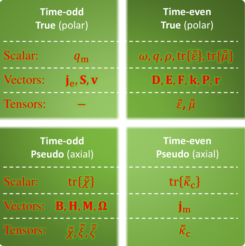
Figure 14: Properties of some electromagnetic scalars, vectors, and tensors with respect to frequency and parity inversions.

Figure 14 richly illustrates the contrast between different material tensors and their space-time symmetry. This information is essential for understanding phenomena which might have similar character but drastically distinct origins. For example, optical rotation effect can be observed in chiral materials and in biased magneto-optical materials, as seen in Fig. 8, however, these effects have a different nature. This difference was understood already by Faraday and commented by Kelvin in his lectures [211].

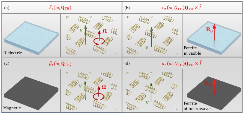
Figure 15: Conceptual implementation of different material tensors. Two characteristic examples are shown for each tensor.

Next, we investigate the properties of material tensors with respect to parity inversion. As it was discussed above, the necessary condition for the existence of nonreciprocal effects in a material is that its response depends on an external parameter which has time-odd symmetry ${\bf Q\mit}_{\rm TO}$. However, in order to achieve nonreciprocal bianisotropic response of a specific type, one should also consider spatial symmetry properties of the material constituents.

Let us consider an arbitrary vector ${\bf a\mit}=a_{x}{\bf x\mit}+a_{y}{\bf y\mit}+a_{z}{\bf z\mit}$ in the Cartesian coordinate system (${\bf x\mit}$, ${\bf y\mit}$, and ${\bf z\mit}$ are the basis unit vectors). Under “active” parity inversion (point reflection), the coordinates of the vector change and the vector in the new system will have form ${\bf a\mit}^{\prime}=-a_{x}{\bf x\mit}-a_{y}{\bf y\mit}-a_{z}{\bf z\mit}=-{\bf a\mit}$. This transformation is equivalent to direction inversion of the vector. Vectors which obey this transformation rule are called true (polar) vectors. Physical vectors such as linear speed ${\bf v\mit}$, force ${\bf F\mit}$, wavevector ${\bf k\mit}$, differential operator $\nabla$, and position vector ${\bf r\mit}$ are true vectors.

Next, let us consider a vector which is a result of the vector product of two true vectors, i.e., ${\bf a\mit}={\bf b\mit}\times{\bf c\mit}$. In the initial physical system, this vector has the form of ${\bf a\mit}=(b_{y}c_{z}-b_{z}c_{y}){\bf x\mit}+(b_{z}c_{x}-b_{x}c_{z}){\bf y\mit}+(b_{x}c_{y}-b_{y}c_{x}){\bf z\mit}$. Under the “active” parity inversion, both true vectors ${\bf b\mit}$ and ${\bf c\mit}$ flip sign (the cross product operation does not change), while their vector product ${\bf a\mit}^{\prime}={\bf b\mit}^{\prime}\times{\bf c\mit}^{\prime}$ remains unchanged, i.e. ${\bf a\mit}^{\prime}={\bf a\mit}$. Thus, vector ${\bf a\mit}$, formed as cross products of two true vectors, transforms differently under parity inversion compared to true vectors. Such vectors are called pseudovectors (axial vectors). Under parity inversion a pseudovector transforms as a true vector with an additional sign flip. It should be noted that the difference in the properties of true vectors and pseudovectors occurs only under parity inversion and does not appear under rotational coordinate transformations. It is easy to check that scalar product of two true vectors gives a true scalar, i.e. a scalar which does not change under parity inversion.

Similarly, it can be shown that a cross product of a true vector and a pseudovector results in a true vector (cross product can be thought as a pseudo-operator itself). An example of pseudovectors in electrodynamics is the magnetic induction vector ${\bf B\mit}$. Indeed, according to ${\bf F\mit}=q{\bf E\mit}+q{\bf v\mit}\times{\bf B\mit}$, the force which is acting on a moving electric charge by the field ${\bf B\mit}$ can be a true vector only if ${\bf B\mit}$ is a pseudovector. Other examples of pseudovectors are magnetic field ${\bf H\mit}$, magnetization ${\bf M\mit}$, and orbital angular velocity vector $\Omega$ (see Fig. 14). From the macroscopic Maxwell equations, it follows that electric field ${\bf E\mit}$, displacement field ${\bf D\mit}$, electric current density ${\bf j\mit}_{\rm e}$ and polarization ${\bf P\mit}$ are all true vectors. Classification to true and pseudo quantities can be extended to scalars and tensors of arbitrary rank assuming that pseudo quantity transforms under parity inversion like a true quantity but with an additional sign flip. True scalars include electric charge $q$, magnetic charge $q_{\rm m}$, frequency $\omega$, electric charge density $\rho$ and the traces (sums of diagonal components) of permittivity and permeability tensors. An example of a pseudoscalar is the trace of chirality tensor ${\rm tr}\{\bar{\bar{\kappa}}\}$. Under parity inversion of chiral isotropic material formed, for example, by helical inclusions, the sign of the chirality parameter of the material changes since the handedness of the helices flips.

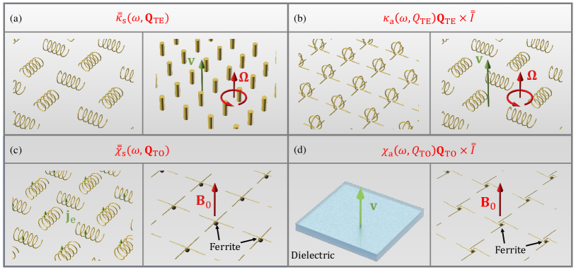
Figure 16: Conceptual implementation of different material tensors. Two characteristic examples are shown for each tensor.

Taking into account the aforementioned parity symmetry properties of the electromagnetic field quantities, let us re-examine constitutive relations (94). One can use the fact that multiplication of a tensor with a vector results in a true vector only if both of them are either true or pseudo quantities. Therefore, one can deduce that $\bar{\bar{{\varepsilon}}}_{\rm r}$, $\bar{\bar{{\varepsilon}}}_{\rm n}$, $\bar{\bar{{\mu}}}_{\rm r}$, and $\bar{\bar{{\mu}}}_{\rm n}$ are true tensors, while $\bar{\bar{{\kappa}}}$ and $\bar{\bar{{\chi}}}$ are pseudotensors. It is convenient to decompose the latter ones to symmetric and antisymmetric parts so that $\bar{\bar{{\kappa}}}=\bar{\bar{{\kappa}}}_{\rm s}+\bar{\bar{{\kappa}}}_{\rm a}$ and $\bar{\bar{{\chi}}}=\bar{\bar{{\chi}}}_{\rm s}+\bar{\bar{{\chi}}}_{\rm a}$. By representing all antisymmetric tensors in the form $\bar{\bar{{\rho}}}(\omega,{{\bf Q\mit}})={{\rho}}(\omega,{Q})\mathbf{Q}\times\bar{\bar{I}}$ (here ${\bf Q\mit}$ is a vector dual to the antisymmetric tensor, $\bar{\bar{I}}$ is a unit tensor and cross product denotes dyadic multiplication), we can summarize the parity symmetry of all the material tensors:

$$\begin{array}[]{lr}\displaystyle\bar{\bar{{\varepsilon}}}_{\rm r}(\omega,\mathbf{Q}_{\rm TE})&{\rm-\,true\,\,tensor},\vspace{1mm}\\ \bar{\bar{{\varepsilon}}}_{\rm n}(\omega,\mathbf{Q}_{\rm TO})={{\varepsilon}}_{\rm n}(\omega,|{Q}_{\rm TO}|)\mathbf{Q}_{\rm TO}\times\bar{\bar{I}}&{\rm-\,true\,\,tensor},\vspace{1mm}\\ \displaystyle\bar{\bar{{\mu}}}_{\rm r}(\omega,\mathbf{Q}_{\rm TE})&{\rm-\,true\,\,tensor},\vspace{1mm}\\ \bar{\bar{{\mu}}}_{\rm n}(\omega,\mathbf{Q}_{\rm TO})={{\mu}}_{\rm n}(\omega,|{Q}_{\rm TO}|)\mathbf{Q}_{\rm TO}\times\bar{\bar{I}}&{\rm-\,true\,\,tensor},\end{array}$$ (102)

$$\begin{array}[]{lr}\displaystyle\bar{\bar{{\kappa}}}_{\rm s}(\omega,\mathbf{Q}_{\rm TE})&{\rm-\,pseudotensor},\vspace{1mm}\\ \bar{\bar{{\kappa}}}_{\rm a}(\omega,\mathbf{Q}_{\rm TE})={{\kappa}}_{\rm a}(\omega,|{Q}_{\rm TE}|)\mathbf{Q}_{\rm TE}\times\bar{\bar{I}}&{\rm-\,pseudotensor},\vspace{1mm}\\ \displaystyle\bar{\bar{{\chi}}}_{\rm s}(\omega,\mathbf{Q}_{\rm TO})&{\rm-\,pseudotensor},\vspace{1mm}\\ \bar{\bar{{\chi}}}_{\rm a}(\omega,\mathbf{Q}_{\rm TO})={{\chi}}_{\rm a}(\omega,|{Q}_{\rm TO}|)\mathbf{Q}_{\rm TO}\times\bar{\bar{I}}&{\rm-\,pseudotensor}.\end{array}$$ (103)

As was mentioned above, the case when there is no external field ${\bf Q\mit}$ acting on the material can be easily taken into account by assuming $Q_{\rm TE}=1$ and ${\bf Q\mit}_{\rm TO}=0$.

Now we have eight tensors each corresponding to specific material response. Each symmetric tensor can be diagonalized in a new basis. Let us note that a symmetric tensor $\bar{\bar{{\rho}}}(\omega,{{\bf Q\mit}})$ is a pseudotensor if one and only one of the two following conditions is correct:

• ${\bf Q\mit}$ is a pseudovector,

• the material has chiral topology (in a sense of broken inversion symmetry).

If one and only one of the two above conditions is correct, an antisymmetric tensor $\bar{\bar{{\rho}}}(\omega,{Q})\mathbf{Q}\times\bar{\bar{I}}$ is, on contrary, a true tensor. Thus, material response attributed to each tensor in (102) and (103) can be achieved by two opposite scenarios: 1) when the external vector ${\bf Q\mit}$ is a true vector; 2) when it is a pseudovector. Figures 15 and 16 summarize all these scenarios (two scenarios for each of the eight material tensors) with some specific known or possible conceptual implementations. It is important to mention that each scenario can be implemented in practice in many different ways, while the figures depict only one of them. Moreover, satisfying the space and time symmetry conditions is a necessary but not sufficient condition to achieve the desired response.

Figure 15a corresponds to realization of material response described by symmetric tensor $\bar{\bar{{\varepsilon}}}_{\rm r}(\omega,\mathbf{Q}_{\rm TE})$. Naturally, such response is realized with simple dielectrics and magnetics without an external bias vector ($Q_{\rm TE}=1$ and ${\bf Q\mit}_{\rm TO}=0$). Another alternative is a medium with broken inversion symmetry on which an external time-even pseudovector acts (simplifying, one can say that the “pseudo symmetry” of the medium in this case is compensated by the pseudovector symmetry, and the permittivity tensor becomes a true tensor). Looking at Fig. 14, one can find that the magnetic current density ${\bf j\mit}_{\rm m}$ is the only example of vector quantity which is time-even and at the same time a pseudovector. However, conceptually, time-even pseudoquantity can be also synthesized by combining two external vectors: Linear speed ${\bf v\mit}$ and orbital angular velocity $\Omega$. In other words, the medium with broken inversion symmetry moving linearly and, simultaneously, rotating around the same direction may also have material tensor $\bar{\bar{{\varepsilon}}}_{\rm r}(\omega,\mathbf{Q}_{\rm TE})$ (see right panel of Fig. 15a).

The antisymmetric permittivity tensor $\bar{\bar{{\varepsilon}}}_{\rm n}(\omega,{\bf Q\mit}_{\rm TO})$ can be achieved with a true time-odd external vector such as linear speed ${\bf v\mit}$ (see Fig. 15b). Note that from (102) it follows that scalar quantity ${{\varepsilon}}_{\rm n}(\omega,|{Q}_{\rm TO}|)$ is time-odd since the entire tensor ${\bar{\bar{{\varepsilon}}}}_{\rm n}$ is time-even. This fact implies that the material response expressed by ${{\varepsilon}}_{\rm n}$ must include some time-odd parameter or time derivative, in addition to the external vector ${\bf Q\mit}_{\rm TO}$. Figure 15b (left side) depicts a conceptual example of a composite which is characterized by tensor $\bar{\bar{{\varepsilon}}}_{\rm n}(\omega,{\bf Q\mit}_{\rm TO})$. The constitutive relations of an isotropic chiral medium (here chirality is required to ensure that $\bar{\bar{{\varepsilon}}}_{\rm n}$ is a true tensor) linearly moving along a given direction contain (in addition to symmetric) an antisymmetric permittivity tensor ${{\varepsilon}}_{\rm n}(v)\mathbf{v}\times\bar{\bar{I}}$, where

$${{\varepsilon}}_{\rm n}(v)=\frac{2j{\kappa}_{\rm i}{\varepsilon}_{\rm i}\left(1-\frac{\displaystyle v^{2}}{\displaystyle c^{2}}\right)/c}{2{\kappa}_{\rm i}^{2}\frac{\displaystyle v^{2}}{\displaystyle c^{2}}\left(1+\frac{\displaystyle v^{2}}{\displaystyle c^{2}}{\varepsilon}_{\rm i}{\mu}_{\rm i}\right)-{\kappa}_{\rm i}^{4}\frac{\displaystyle v^{4}}{\displaystyle c^{4}}-\left(\frac{\displaystyle v^{2}}{\displaystyle c^{2}}{\varepsilon}_{\rm i}{\mu}_{\rm i}-1\right)^{2}}$$ (104)

and ${\varepsilon}_{\rm i}$, ${\mu}_{\rm i}$, and ${\kappa}_{\rm i}$ stand for isotropic permittivity, permeability and chirality parameter of the medium when it is at rest. We have derived this nontrivial result from [116, Sec. 3.4.2]. It is easy to see that scalar function ${{\varepsilon}}_{\rm n}(v)$ in fact includes a time derivative ($j\kappa_{\rm i}$ is equivalent to $j\omega\kappa_{\rm c}$ according to (100)), as required by the time-reversal symmetry. Another and more traditional way to achieve the antisymmetric permittivity is based on biasing magneto-optical materials with a time-odd pseudovector field, namely magnetic flux density ${\bf B\mit}_{0}$ (see the right panel of Fig. 15b). To satisfy the time-reversal symmetry, the scalar function ${{\varepsilon}}_{\rm n}$ includes a time derivative ($j\omega$ in the frequency domain), as is seen in (87) for the off-diagonal permittivity components. Alternatively, similar effect was reported using another pseudovector bias field, orbital angular velocity $\Omega$, and was coined as “rotatory ether drag” in a rapidly rotating rod made of Pockels glass [212]. This is an analogue of Faraday rotation without external magnetic field.

The symmetric and antisymmetric parts of the permeability tensor can be synthesized using the same techniques as those for the permittivity tensor (see Figs. 15c and d). The only difference is that the antisymmetric part resulted from magnetic biasing occurs due to the ferromagnetic resonance at microwaves, rather than electron cyclotron orbiting at optical frequencies.

Figure 16a (left panel) depicts a typical implementation of the symmetric chirality tensor $\bar{\bar{{\kappa}}}_{\rm s}(\omega,{\bf Q\mit}_{\rm TE})$ via a random mixture of metal helices (so-called Pasteur medium). This realization does not require external bias ($Q_{\rm TE}=0$). Another interesting route is based on a time-even pseudovector quantity originated via linear velocity ${\bf v\mit}$ and simultaneous angular velocity $\Omega$. Interestingly, in this case the material constituents can be achiral (such as conceptual cylinders shown in right panel of Fig. 16a), chirality is generated solely through the external bias quantities [105, Sec. 1.9.5, Fig. 1.21]. Another route to achieve chirality is a gyrotropic (biased magneto-optical) medium moving linearly with speed ${\bf v\mit}$ in the direction of the bias [128, § 7.4c],[213, § 5].

The antisymmetric tensor $\bar{\bar{{\kappa}}}_{\rm a}$ can be gained without an external field in an achiral so-called omega medium in which ${\bf Q\mit}_{\rm TE}={\bf r\mit}$ (description of the constituent geometry and scattering physics behind can be found e.g. in [125]) or, potentially, in a chiral medium moving linearly and rotating around the same axis (see Fig. 16b).

Nonreciprocal symmetric material tensor $\bar{\bar{{\chi}}}_{\rm s}(\omega,{\bf Q\mit}_{\rm TO})$ might be achieved in a medium with broken inversion symmetry biased by some external time-odd true vector field. It is worth mentioning that a chiral medium moving with linear speed ${\bf v\mit}$, although is satisfies the symmetry requirements (103), in fact does not possess Tellegen coupling. This confirms our previous remark that the symmetry conditions are necessary but not sufficient. Probably, a chiral medium biased by external electric current ${\bf j\mit}_{\rm e}$ could generate response in form of $\bar{\bar{{\chi}}}_{\rm s}(\omega,{\bf Q\mit}_{\rm TO})$ (see Fig. 16c). The second and feasible route is based on achiral media with ferrite-based constituents biased by pseudovector external magnetic flux density ${\bf B\mit}_{0}$ [214], as shown in the right panel of Fig. 16c. It is so far, probably, the most practical implementation of artificial Tellegen medium proposed in [139]. Magnetoelectric properties of Tellegen type appear also in natural materials, such as topological insulators [215] and multi-ferroic media [216].

Finally, the antisymmetric tensor $\bar{\bar{{\chi}}}_{\rm a}$ can be attained in a moving isotropic dielectric medium with linear speed ${\bf v\mit}$ [128, Sec. 7.4a],[217] or in a chiral medium biased by an external pseudovector such as magnetic flux density ${\bf B\mit}_{0}$ (see Fig. 16d). Interesting alternatives to the first approach were proposed based on dielectric scatterers rotating with angular speed ${\bf v\mit}=\Omega\times{\bf r\mit}$ [218, 219, 220] (${\bf v\mit}$ is a true vector), based on synthetic motion [221], and based on materials biased by static electric and magnetic fields which are orthogonal to one another and to the light wavevector, resulting in $\bar{\bar{{\chi}}}_{\rm a}$ being proportional to ${\bf E\mit}\times{\bf B\mit}$ [222, 223, 224] (${\bf E\mit}\times{\bf B\mit}$ is a true vector). Structures with antisymmetric tensor $\bar{\bar{{\chi}}}_{\rm a}$ were proposed in optical [225, 226] and microwave [214, 227, 228] regimes and experimentally demonstrated in works [229, 224, 230]. Recently, the effect of similar symmetry type was proposed for phonons [231].

Thus, space and time inversion symmetries are powerful tools for analyzing and designing materials with arbitrary electromagnetic properties, which can be required by various applications. One of the early examples of exploiting symmetry arguments for obtaining new results can be found in [232]. Space and time inversion symmetries provide a simple but fundamental classification of all possible linear effects in matter. Moreover, this approach allows us to draw analogies between seemingly distinct effects which have the same physical origin.

VI Nonreciprocity in nonlinear systems

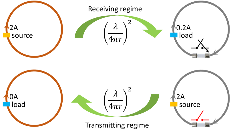
Figure 17: Nonreciprocal communication between two small loop antennas. The loop antenna on the right side includes a nonlinear device (electrical fuse) for controlling the magnitude of the electric current flowing through the loop. Here, $r$ is the distance between the two antennas and $\lambda$ denotes the operating wavelength in free space.

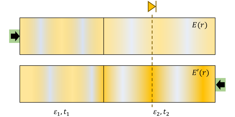
Figure 18: Forward (up) and backward (bottom) wave propagation through an infinitely-wide slab consisting of two layers of thicknesses $t_{1}$ and $t_{2}$. The regions outside the slab are assumed to be vacuum. The gradient color shows the magnitude of the total electric field $E(r)$ inside the slab. The dashed line shows the location where the ratio of the total fields for the forward and backward illuminations is the maximum. By positioning a nonlinear element at this location, one can achieve nonreciprocal wave transmission through the slab.

Nonlinearity can be used to break the Lorentz reciprocity, and therefore, gives an opportunity for manipulation of the transmission characteristics of systems in order to design nonreciprocal components [21, 22, 23, 24, 25, 26, 27, 28, 29, 30, 31, 32, 33, 34, 35, 36, 37, 38, 39, 40, 41, 42, 43, 44, 45, 46, 47, 48, 49, 50, 51, 52, 53]. Nonlinear nonreciprocal devices exploit the fact that field distributions in direct and reciprocal processes can be very different. The main idea is to position nonlinear objects where the field strength is high for one propagation direction and weak for the opposite one.

Perhaps the simplest example is coupling between two small antennas in free space as shown in Fig. 17. We consider two loop antennas whose radii are much smaller than the free-space wavelength, and they are separated by a sufficient distance. One of the antennas (the right one in Fig. 17) is connected to a nonlinear object (here, an electrical fuse as the simplest conceptual example) which is sensitive to the magnitude of the electric current flowing through the loop. If the current magnitude is large enough, the object works similarly to a switch and opens the circuit, while it is short-circuited if the current magnitude is not high. In the receiving regime, when the right antenna is a receiver, the induced electric current is small due to the free-space path loss $[\lambda/(4\pi r)]^{2}$ despite the magnitude of the transmitting current is considerably large. Therefore, the nonlinear object is short circuited and the load receives the electric power. However, in the transmitting regime (when the right antenna is transmitting), since the magnitude of the transmitting current is large, the nonlinear object is consequently open circuited, and no energy is transferred to the load in the left loop antenna. Thus, one could simply design a nonreciprocal link between the two antennas by using the concept of nonlinearity.

In the above example, we had the free-space path loss causing the attenuation of energy and ensuring the asymmtetry of the field distribution. However, it is also possible to design a nonreciprocal system where there is no power spread, like a nonreciprocal waveguide. To understand the principle of nonreciprocal isolators in waveguides, let us discuss an explicit example [46]. Consider a double slab which is extended infinitely in the transverse plane and has a finite thickness in the longitudinal direction. It comprises two dielectric layers made of isotropic linear materials which have contrasting relative permittivities $\varepsilon_{1}$ and $\varepsilon_{2}$. In addition, the thicknesses of those layers can be also different, namely $t_{1}$ and $t_{2}$ (see Fig. 18). Due to such nonidentical permittivities and thicknesses, the whole system is spatially asymmetric. This asymmetry plays the key role for obtaining nonreciprocity. Illuminating the double slab by an incident wave, we excite a standing wave within the slab (meaning that there are maxima and minima for the amplitude of the field). However, intriguingly, such standing waves are different for forward and backward illuminations, and the spatial distribution of the field inside the slab is, indeed, dependent on the propagation direction of the input wave, as is shown with gradient color in Fig. 18. While we certainly achieve the same transmission coefficient as the system is reciprocal by this point, the field distribution inside the slab is not the same. As a consequence, there exist locations at which the ratio between the local fields induced by two incident waves illuminated from opposite sides, is high. Next, to complete the design of a nonlinear isolator, let us place a nonlinear resonant element at the location where the ratio is maximum (shown by the dashed line in the figure). Since the performance of the element depends on the field amplitude, its interaction with the field in the two cases (illuminations from the right and from the left side) will be dramatically different. For that reason, by proper design of the system, noticeable transmission for one direction and low transmission for the opposite direction can be attained. Importantly, nonlinearity must be accompanied by the spatial asymmetry to break the Lorentz reciprocity.

However, these conditions cannot provide us with an ideal nonreciprocity, and in practice nonlinear isolators face limitations. The above explanations were based on assumption that the forward and backward incident waves are not concurrently present. Let us give another example to understand the problem. Now, the system consists of a single dielectric layer. The dielectric is nonhomogeneous (to provide necessary spatial asymmetry) and described by permittivity ${\varepsilon}({\bf r\mit})$ for weak excitations and by ${\varepsilon}({\bf r\mit})+\Delta{\varepsilon}({\bf r\mit},E)$ for incident waves with strong fields (in the nonlinear regime). Naturally, for weak excitations, the layer will exhibit reciprocal transmission for forward and backward illuminations, as shown in Fig. 19(a–b). The field distribution will be different in the two cases, similarly to Fig. 18. For strong excitations, nonlinear dielectric polarization will occur, causing different transmission levels for opposite illuminations (see Fig. 19(c–d)). High isolation can be achieved by designing specific distribution of ${\varepsilon}({\bf r\mit})$. Consider that the dielectric layer is illuminated by a low-power incident wave together with the a high-power wave (the two waves propagate in the same forward direction). In this case, the low-power wave will have the same high transmission, like in Fig. 19(c).

Now, let us assume that an input high-power wave illuminates the dielectric layer in the forward direction, while, at the same time, a low-power wave is incident on it from the backward direction. The question is whether the low-power wave will pass through (like in Fig. 19(b)) or be blocked by the layer (like in Fig. 19(d)). In fact, it will pass through since in the presence of the high-power wave, the polarization induced by the low-power wave will linearly depend on its electric field. This effect was known in the microwave community for long time in electronic diodes, which are essentially nonlinear systems, as “small-signal approximation” [233, § 3.3.8]. In photonics, the effect was proposed recently and coined as “dynamic reciprocity” [44]. Next, we will provide derivations explaining the origin of the effect. According to nonlinear optics, the wave equation inside nonlinear nonhomogeneous dielectric can be written in the form [234, eq. (2.1.21)],[44]:

$$\nabla\times\nabla\times\mathbf{\tilde{E}}+\mu_{0}\varepsilon_{0}{\varepsilon}(\mathbf{r}){\partial^{2}\mathbf{\tilde{E}}\over\partial t^{2}}+\mu_{0}{\partial^{2}\mathbf{\tilde{P}}_{\rm NL}\over\partial t^{2}}=0,$$ (105)

where $\mathbf{\tilde{E}}$ is the time-harmonic electric field, ${\varepsilon}$ is the frequency dependent permittivity in the linear regime, and $\mathbf{\tilde{P}}_{\rm NL}$ denotes the nonlinear polarization density vector which in the general case depends on the electric field as [234, eq. (1.1.2)]

$$\mathbf{\tilde{P}}_{\rm NL}=\varepsilon_{0}{\chi}^{(2)}(\mathbf{r})\mathbf{\tilde{E}}^{2}+\varepsilon_{0}{\chi}^{(3)}(\mathbf{r})\mathbf{\tilde{E}}^{3}+\dots$$ (106)

Here, ${\chi}^{(n)}(\mathbf{r})$ is the $n$-th order component of the electric susceptibility of the medium. Let us consider the optical (AC) Kerr nonlinearity. For media which have a significant Kerr effect, the third-order component ${\chi}^{(3)}$ is dominant and the other components are neglected, i.e. $\mathbf{\tilde{P}}_{\rm NL}\approx\varepsilon_{0}{\chi}^{(3)}(\mathbf{r})\mathbf{\tilde{E}}^{3}$.

Since in our example, the dielectric layer is illuminated by the high-power and low-power waves simultaneously, the total electric field can be written as $\mathbf{\tilde{E}}=\mathbf{{E}}_{\rm{h}}\exp(j\omega_{\rm{h}}t)+\mathbf{{E}}_{\rm{l}}\exp(j\omega_{\rm{l}}t)$, in which $|\mathbf{{E}}_{\rm{h}}|\gg|\mathbf{{E}}_{\rm{l}}|$ are the complex amplitudes of the time-harmonic waves. The frequencies of the two waves $\omega_{\rm{h}}$ and $\omega_{\rm{l}}$ are different. Note that the dynamic reciprocity restriction is not applied when $\omega_{\rm{h}}$ and $\omega_{\rm{l}}$ are equal since the resulting linearized equation is nonreciprocal [44, Suppl. Inf.],[48]. After substituting $\mathbf{\tilde{E}}$ in the expression for $\mathbf{\tilde{P}}_{\rm NL}$ and doing some algebraic manipulations, one obtains [234, eq. (4.1.12)],[44]

$$\mathbf{\tilde{P}}_{\rm NL}\approx\mathbf{\tilde{P}}_{0}+\mathbf{\tilde{P}}_{\omega_{\rm{l}}}=\mathbf{\tilde{P}}_{0}+6\varepsilon_{0}{\chi}^{(3)}(\mathbf{r})|\mathbf{{E}}_{\rm{h}}|^{2}\mathbf{{E}}_{\rm{l}}{\rm e}^{j\omega_{\rm l}t},$$ (107)

where $\mathbf{\tilde{P}}_{\omega_{\rm{l}}}$ is the polarization density due to the low-power incident wave and $\mathbf{\tilde{P}}_{0}$ is the rest of the polarization terms oscillating at different frequencies. It is clear that the above equation is a linear equation for the low-power incident wave with frequency $\omega_{\rm{l}}$. It provides a linear susceptibility which is proportional to the third-order susceptibility and to the square of the magnitude of the high-power signal. Put another way, one can introduce the effective susceptibility as $\mathbf{\tilde{P}}_{\omega_{\rm{l}}}=\varepsilon_{0}{\chi}_{\omega_{\rm{l}}}\tilde{{\bf E\mit}}_{\rm l}$, where

$${\chi}_{\omega_{\rm{l}}}\approx 6{\chi}^{(3)}(\mathbf{r})|\mathbf{{E}}_{\rm{h}}|^{2}.$$ (108)

Note that (107) is physically equivalent to Eq. (3.15) in [233] written in terms of the current and voltage for electronic diodes. That equation implies that a low-amplitude current flowing through the diode in the presence of a high-amplitude current will “sense” the diode as a simple linear resistance.

Having (107) in mind, in the frequency domain, we can rewrite (105) as a linearized equation for the low-power incident wave

$$\nabla\times\nabla\times\mathbf{{E}}_{\rm{l}}-k^{2}_{\rm{l}}\Big{[}{\varepsilon}(\mathbf{r})+6{\chi}^{(3)}(\mathbf{r})|\mathbf{{E}}_{\rm{h}}|^{2}\Big{]}\mathbf{{E}}_{\rm{l}}=0,$$ (109)

where $k_{\rm{l}}=\omega_{\rm{l}}\sqrt{\mu_{0}\varepsilon_{0}}$ is the free-space wave number. We conclude that the effective relative permittivity corresponding to this linear equation is indeed equal to ${\varepsilon}_{\rm eff}(\mathbf{r})={\varepsilon}(\mathbf{r})+6{\chi}^{(3)}(\mathbf{r})|\mathbf{{E}}_{\rm{h}}|^{2}$. Since the dielectric function ${\varepsilon}_{\rm eff}$ is scalar and time-independent, propagation of the low-power incident wave will be reciprocal. Therefore, it will not be blocked by the layer during the backward illumination. Such functionality precludes the described nonlinear system from operating as an ideal isolator.

In addition to the considered constraint, the nonreciprocity via nonlinearity has another fundamental limitation due to the second law of thermodynamics [235, 53]. Accordingly, the nonlinear isolators cannot operate from both sides simultaneously. It can be readily expected that if such an isolator could operate, the radiative thermal power transferred between the ports would not be zero while the two ports are kept in the same temperature. This violates the second law of thermodynamics which stresses that the total radiative power transferred must be zero. For linear isolators, for example, we do not have this limitation because the power illuminated from one of the isolated port is absorbed [235]. Finally, in [236, 53] the third limitation was pointed out. It states that there is a tradeoff between transmission in the forward direction and the level of input intensity for which large isolation (in an isolator) can be obtained. This limitation comes from the fact that the field asymmetry reduces when the transmission through the structure increases [47]. It is worth mentioning that similar conclusions were obtained in [90, § XXI].

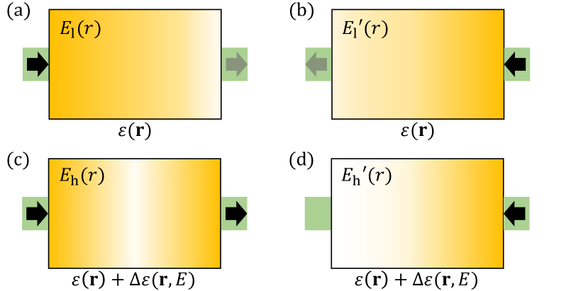
Figure 19: The general schematic view of a nonreciprocal device based on a nonlinear dielectric slab. The slab is spatially asymmetric and is described by linear permittivity ${\varepsilon}({\bf r\mit})$ for weak excitations and by nonlinear permittivity ${\varepsilon}({\bf r\mit})+\Delta{\varepsilon}({\bf r\mit},{E})$ for strong excitations. The gradient color shows the magnitude of the total electric field ${E}(r)$ inside the slab. (a–b) Illuminations from different sides by a low-power wave (reciprocal transmission). (c–d) Same for a high-power wave (nonreciprocal transmission).

VII Nonreciprocity in linear time-variant systems

An alternative approach for breaking reciprocity, without using magnetic or nonlinear materials, is to break the time-invariance of the system. The possibility of using time-variant systems (also called time-modualted), has been known for many years [58, 59, 60, 61, 62, 63, 64, 65, 66, 67, 237, 238, 239]. However, due to the technological advances on the implementation of time-variant systems, it has been in the recent years when these solutions have been proposed for the design of compact nonreciprocal devices [68, 69, 70, 71, 72, 73, 74, 75, 76, 77, 78, 79, 80, 81, 82, 83, 84, 85, 86, 94, 95].

Before discussing these methods we need to clarify the definition of reciprocal and nonreciprocal processes for time-varying systems. Processes in time-invariant systems are called reciprocal if the two reaction integrals are equal, see (40). In the frequency domain, for a two-port device, we simply have the symmetry relation for the S-parameters $S_{12}=S_{21}$. For time-varying systems, the definition of reciprocity should be given in time domain. It is usually formulated in terms of equality of convolution integrals (68) or correlation integrals [135, 66, 134]. However, especially for harmonic pumping, the use of this general definition is not convenient.

Next, we derive reciprocity relations in systems whose material properties vary harmonically with time. We consider a special case when the permittivity of the background material is globally modulated according to the following symmetric (with respect to time) modulation function

$${\varepsilon}(\omega,{\bf r\mit},t)={\varepsilon}_{\rm st}(\omega,{\bf r\mit})+M({\bf r\mit})\cos(\Omega t+\phi),$$ (110)

where $\tilde{\varepsilon}_{\rm st}$ is the static permittivity, $M({\bf r\mit})$ is the modulation strength function, $\Omega$ is the modulation frequency, and $\phi$ is an arbitrary phase. Here, for simplicity, we use the adiabatic model for temporal modulations, assuming that the operational frequency $\omega$ is very low compared to the lowest resonance frequency of the material. Note that this model can be used for arbitrary modulation frequency $\Omega$ (see  [240],[241, Suppl. Inf.] for details). In the general non-adiabatic case, the following derivations could still be performed, writing the material parameters using integrals over past time. Here, for simplicity, we assume that $M({\bf r\mit})$ has no frequency dispersion. This assumption is realistic for gaseous plasmas with properly modulated in time charge concentration $N_{\rm e}(t)$ [240, Eq. (53)]. The reciprocity relation which we discuss below, however, can be derived also for other models of the modulation function. The permeability is assumed to be static in time. Global modulation implies that at all points in space the permittivity alternates with the same phase. Frequency-domain wave equation for the time-varying material reads [242]

$$\nabla\times\frac{1}{{\mu}(\omega)}\nabla\times{{\bf E\mit}}-\omega^{2}\left[{\varepsilon}_{\rm st}(\omega){{\bf E\mit}}+{{\bf P\mit}}_{\rm M}\right]=-j\omega{{\bf J\mit}},$$ (111)

where the spatial dependency is assumed implicitly and ${{\bf P\mit}}_{\rm M}(\omega)$ is the additional polarization density of the material due to dynamic modulation which can be found from (110):

$${{\bf P\mit}}_{\rm M}(\omega)=\frac{M}{2}\left[{\rm e}^{j\phi}{{\bf E\mit}}(\omega-\Omega)+{\rm e}^{-j\phi}{{\bf E\mit}}(\omega+\Omega)\right].$$ (112)

Modulation of the permittivity at a frequency $\Omega$ induces a number of sideband field harmonics ${{\bf E\mit}}_{n}$ of frequencies $\omega_{n}=\omega_{0}+n\Omega$, where $n$ is an integer. This is due to the periodicity of the electric field which is the solution of wave equation (111) and can be written in terms of the Fourier series. Substituting (112) in (111) and matching specific frequency components with temporal ${\rm e}^{j\omega t}$ variations, one can obtain wave equation in the form

$$\hat{\Theta}_{n}{{\bf E\mit}}_{n}-\omega_{n}^{2}\frac{M}{2}\left[{\rm e}^{j\phi}{{\bf E\mit}}_{n-1}+{\rm e}^{-j\phi}{{\bf E\mit}}_{n+1}\right]=-j\omega_{n}{{\bf J\mit}}_{n}.$$ (113)

Here, $\hat{\Theta}_{n}$ is an operator defined through its action: $\hat{\Theta}_{n}{{\bf E\mit}}_{n}=\nabla\times\frac{1}{{\mu}_{n}}\nabla\times{{\bf E\mit}}_{n}-{\varepsilon}_{{\rm st},n}\omega_{n}^{2}{{\bf E\mit}}_{n}$. For generality, we assume a current source with multiple side bands, with ${{\bf J\mit}}_{n}$ denoting the source at frequencies $\omega_{n}=\omega_{0}+n\Omega$. It can be shown that writing (113) in the matrix form and expressing electric field vector as ${{\bf E\mit}}_{n}=\overline{\overline{f}}_{nm}{{\bf J\mit}}_{m}$, we always obtain asymmetric matrix $\overline{\overline{f}}$. However, by dividing both sides of (113) by $\omega_{n}^{2}$ and using replacement ${{\bf J\mit}}^{\prime}_{m}={{\bf J\mit}}_{m}/\omega_{m}$, we obtain relation

$${{\bf E\mit}}_{n}({\bf r\mit})=\overline{\overline{F}}_{nm}({\bf r\mit}){{\bf J\mit}}^{\prime}_{m}({\bf r\mit}),$$ (114)

where $\overline{\overline{F}}$ is a symmetric matrix if $\phi=0$ is chosen. Note that phase $\phi$ can be chosen arbitrarily by time translation $t\rightarrow t+\Delta t$ [72]. Formally solving (114), the radiated field harmonics by given current source read as

$${{\bf E\mit}}_{n}({\bf r\mit})=\int_{V}\bar{\bar{{G}}}_{nm}({\bf r\mit},{\bf r\mit}^{\prime}){{\bf J\mit}}^{\prime}_{m}({\bf r\mit}^{\prime}){\rm d}V^{\prime}.$$ (115)

Since $\overline{\overline{F}}$ is symmetric, dyadic Green’s function of time-varying material is also symmetric

$$\overline{\overline{G}}({\bf r\mit},{\bf r\mit}^{\prime})=\overline{\overline{G}}^{T}({\bf r\mit},{\bf r\mit}^{\prime}).$$ (116)

Here ${\bf r\mit}^{\prime}$ denotes coordinates of points inside source volume $V$. Comparing (115) and (116) to (31) and (34), we see that electromagnetic radiation in time-varying material with global modulation (110) satisfies the Onsager reciprocity conditions, i.e. is always reciprocal. The important difference between (31) and (115) is that in the latter case the current harmonics are normalized by their frequencies. Repeating derivations analogous to (42) and (43), we obtain equation

$$\int\limits_{V_{A}}\sum_{n}\frac{{{\bf E\mit}}_{n}^{(B)}\cdot{{\bf J\mit}}_{n}^{(A)}}{\omega_{n}}{\rm d}V_{A}=\int\limits_{V_{B}}\sum_{n}\frac{{{\bf E\mit}}_{n}^{(A)}\cdot{{\bf J\mit}}_{n}^{(B)}}{\omega_{n}}{\rm d}V_{B},$$ (117)

which relates the fields and current harmonics generated via interaction between a pair of two sources $A$ and $B$ (similarly to the scenario shown in Fig. 7). Relation (117) is the electromagnetic reciprocity theorem for time-varying systems. Let us write (117) for the special case when each current source is represented by one frequency harmonic, i.e. ${{\bf J\mit}}_{n}^{(A)}={{\bf J\mit}}_{p}^{(A)}\delta_{pn}$ and ${{\bf J\mit}}_{n}^{(B)}={{\bf J\mit}}_{q}^{(B)}\delta_{qn}$:

$$\int\limits_{V_{A}}\frac{{{\bf E\mit}}_{p}^{(B)}\cdot{{\bf J\mit}}_{p}^{(A)}}{\omega_{p}}{\rm d}V_{A}=\int\limits_{V_{B}}\frac{{{\bf E\mit}}_{q}^{(A)}\cdot{{\bf J\mit}}_{q}^{(B)}}{\omega_{q}}{\rm d}V_{B}.$$ (118)

When $p=q$ (sources $A$ and $B$ are at the same frequency), equation (118) simplifies to the conventional form of reciprocity theorem (40). In the case when $p=1$ and $q=2$ and ${{\bf J\mit}}^{(A)}(\omega_{1})={{\bf J\mit}}^{(B)}(\omega_{2})$, the radiated fields harmonics are not equal ${{\bf E\mit}}^{(A)}(\omega_{2})\neq{{\bf E\mit}}^{(B)}(\omega_{1})$, differing by the ratio of frequencies $\omega_{1}/\omega_{2}$ (for uniform current sources). Reciprocity relation (118) applies restriction on how a two-port device converts waves of $\omega_{1}$ into $\omega_{2}$ in the forward direction and $\omega_{2}$ into $\omega_{1}$ in the backward direction: The conversion efficiencies of these two processes are not equal and must be related through $\omega_{1}$ and $\omega_{2}$. It is important to note that (117) does not impose direct constraints on the identical conversions from $\omega_{1}$ into $\omega_{2}$ (in the forward direction) and from $\omega_{1}$ into $\omega_{2}$ (in the backward direction).

Reciprocity relation (117) connects reaction functions normalized by frequencies or, alternatively, energies of photons if we divide both sides of the relation by the reduced Planck constant $\hbar$. Thus, the fractions inside the volume integrals have dimensions of photon number flux (number of photons per second per unit area). In other words, reciprocity implies restriction on the evolution of number of photons in the direct and inverse processes, rather than intensities of waves. Analogous observation can be applied to the Manley-Rowe relations for nonlinear processes [234, § 2.5].

Thus, we have concluded that systems with global symmetric time-harmonic modulation of permittivity (110) are always reciprocal in the sense that relation (117) is always satisfied. Interestingly, although such systems break time-reversal symmetry of Maxwell equations (since $\tilde{\varepsilon}(-t)\neq\tilde{\varepsilon}(t)$ for given $\phi$), they obey the so-called generalized time-reversal symmetry expressed as $\tilde{\varepsilon}(-t+t_{0})=\tilde{\varepsilon}(t+t_{0})$ [97]. For any given $\phi$, it is always possible to find such value of $t_{0}$ that the above equality holds.

If modulation is not global and can be represented by two modulation functions [72]

$$\tilde{\varepsilon}(\omega,{\bf r\mit},t)=\tilde{\varepsilon}_{\rm st}(\omega,{\bf r\mit})+M_{1}({\bf r\mit})\cos(\Omega t+\phi_{1})+M_{2}({\bf r\mit})\cos(\Omega t+\phi_{2})$$ (119)

with $\phi_{1}\neq\phi_{2}$ and $M_{1}({\bf r\mit})\neq\alpha M_{2}({\bf r\mit})$ ($\alpha$ is an arbitrary real constant), then equation (113) cannot be written in the form ${{\bf E\mit}}_{n}({\bf r\mit})=\overline{\overline{F}}_{nm}({\bf r\mit}){{\bf J\mit}}^{\prime}_{m}({\bf r\mit})$ with $\overline{\overline{F}}$ being symmetric matrix (time translation affects both $\phi_{1}$ and $\phi_{2}$ and does not make $\overline{\overline{F}}$ symmetric). Therefore, dyadic Green’s function is asymmetric, and this time-modulated system will break reciprocity relation (117). Nevertheless, one can write Onsager-Casimir relation which imposes constraint even on time-modulated nonreciprocal systems:

$$\int\limits_{V_{A}}\sum_{n}\frac{{{\bf E\mit}}_{n}^{(B)}(\Omega)\cdot{{\bf J\mit}}_{n}^{(A)}}{\omega_{n}}{\rm d}V_{A}=\int\limits_{V_{B}}\sum_{n}\frac{{{\bf E\mit}}_{n}^{(A)}(-\Omega)\cdot{{\bf J\mit}}_{n}^{(B)}}{\omega_{n}}{\rm d}V_{B}.$$ (120)

Here, similarly to (41), the argument $-\Omega$ implies that the corresponding quantity should be considered in the medium with time modulation reversed, i.e. assuming $t\rightarrow-t$ in (119) or, equivalently, reversing signs of $\phi_{1}$ and $\phi_{2}$. This result is apparent from equality $\overline{\overline{F}}({\bf r\mit},{\bf r\mit}^{\prime},\Omega)=\overline{\overline{F}}^{T}({\bf r\mit},{\bf r\mit}^{\prime},-\Omega)$.

It is important to note that reciprocity can be broken even in globally (uniformly) modulated systems which include materials whose properties vary according to an asymmetric function (e.g., with sawtooth profile) [97] or bianisotropic materials with varying magnetoelectric coupling (even with symmetric variation profile). The latter scenario can be verified following derivations (111)–(113) and using bianisotropic constitutive relations (60). For example, in [241], strong nonreciprocity was reported for a single bianisotropic metasurface of the “omega” type with uniform time modulation. Figure 20 summarizes the Lorentz reciprocity relations and Onsager-Casimir relations for time-invariant and time-varying materials.

Next, we present two main approaches for creation of nonreciprocal devices based on time modulation.

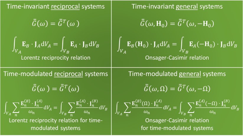
Figure 20: Summary of the Lorentz reciprocity relations (for reciprocal electromagnetic systems) and Onsager-Casimir relations (for both reciprocal and nonreciprocal systems) for time-invariant and time-varying materials. The time-modulated system is called reciprocal if the Lorentz reciprocity relation holds for some specific time translation $\Delta t$.

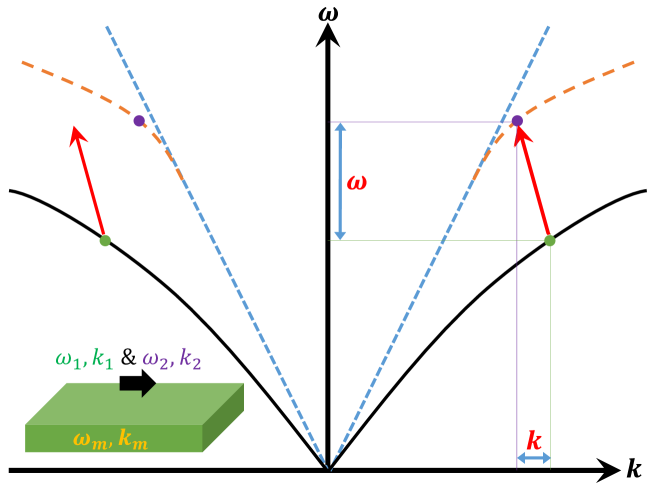
Figure 21: The dispersion curve for a waveguide supporting two different modes. If waveguide’s dielectric constant is spatially and temporally modulated with the frequency $\omega_{\rm{m}}$ and the momentum $k_{\rm{m}}$, an indirect wave transition happens. This transition is the key point in achieving different transmission from opposite ports.

VII-1 Travelling-wave modulation

It is clear that studies and applications of travelling-wave modulations have a long history at least in microwave engineering. It appears that this concept was developed in 1950s and 1960s for parametric amplifiers [58]. It is known that for a lossless transmission line with a distributed inductance per unit length $L=L_{0}+M\sin 2(\omega t-kz)$, the amplitude of the current wave is exponentially growing or decaying. Precise synchronization between the oscillator (which produces the variation of the inductance in time) and the incoming signal gives rise in maximum possible amplification. A simple pictorial example of such synchronization is a child at a playground swing. The child “pumps” the swing by periodically standing and squatting to increase the amplitude of the swing’s oscillations. The maximum efficiency is achieved when the ”pump” motions is at twice the frequency of swing’s oscillations [243].

Travelling-wave modulation for achieving nonreciprocity (in contrast to amplification) has recently attracted strong attention of researchers. In analogy with the above description of parametric amplifiers, let us consider an inhomogeneous isotropic dielectric waveguide with permittivity [68]

$$\tilde{\varepsilon}(x,y,z,t)=\varepsilon_{\rm st}(x,y)+M(x,y)\cos(\omega_{\rm{m}}t-k_{\rm{m}}z).$$ (121)

Here, $\varepsilon_{\rm st}(x,y)$ denotes the static permittivity, $M(x,y)$ is the modulation amplitude distribution, $\omega_{\rm{m}}$ represents the modulation angular frequency, $k_{\rm{m}}$ is the modulation wave number, and finally $z$ is the axis of propagation inside the waveguide. We suppose that the modulation frequency is small compared to the frequency of the wave signal. The dielectric waveguide supports two oppositely propagating modes whose angular frequencies $\omega_{1}$ and $\omega_{2}$ correspond to the phase constants $k_{1}$ and $k_{2}$, respectively. Regarding the forward direction, if the difference between the two angular frequencies is equal to the modulation angular frequency, i.e. $\omega_{\rm{m}}=\omega_{2}-\omega_{1}$, and if also the same condition holds for the phase constants $k_{\rm{m}}=k_{1}-k_{2}$, an indirect photonic transition happens (see Fig. 21). Accordingly, the first mode fully transits to the second mode. Such mode conversion is found to be made after propagation over a distance (called coherence length [68]). It should be mentioned that the modulation frequency can be much smaller than the carrier frequency of the input signal. If the above strict conditions are not obeyed, the conversion will not happen and the modulation does not influence the incoming signal, as is shown in Fig. 21. Indeed, this is the true scenario related to the backward direction. Remind that for the backward propagation the phase constants along the waveguide are $-k_{1}$ and $-k_{2}$. Therefore, due to the spatiotemporal modulation, both time-reversal symmetry and spatial-inversion symmetry are broken, and the system becomes nonreciprocal. From microwave engineering point of view, this is similar to inserting properly modulated capacitors in a transmission line. Such a line offers nonreciprocal propagation [78].

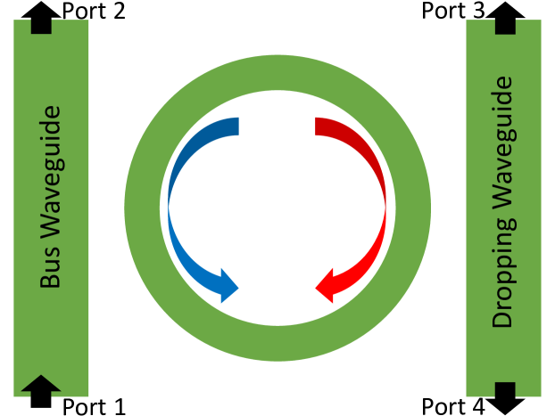
Figure 22: An add-drop filter based on a ring resonator. Azimuthal spatiotemporal modulation of the ring resonator removes the degeneracy between the two modes of opposite handedness in the modulated ring. The input signal from port 1 is not transmitted to port 2, while the signal is fully transmitted to port 1 when it is incident from port 2. In the case of no modulation, the degeneracy exists and the transmission coefficients $S_{21}$ and $S_{12}$ are identical.

VII-2 Angular momentum

Let us consider a simple example of a circular cavity which is accompanied with a waveguide structure [89], as shown in Fig. 22. Here, the ring cavity is located between two parallel waveguides. This ring resonator simultaneously supports two modes propagating in the opposite directions: Righ-handed and left-handed modes. The parallel waveguides are coupled to the resonator. Accordingly, if the frequency of the incident signal from the waveguide port is the same as the resonance frequency of the resonator, the transmission coefficient (from the input port 1 to the output port 2) will be zero. At other frequencies, full transmission occurs. The more important point is that the dip in the transmission for both modes is identical giving rise to a reciprocal structure since $S_{12}=S_{21}$ ($S$ denotes the scattering matrix). However, if the degeneracy of these two counterpropagating modes is revoked, we can create a nonreciprocal response. When the degeneracy is lifted, the resonance frequency of the cavity is different for the two modes. Consequently, the transmission coefficients $S_{12}$ and $S_{21}$ are not equal. One way to obtain different resonance frequencies is to use magnetic (or magneto-optical) materials which will result in different guided wavelengths for opposite propagation directions. However, similarly to the previous approach for achieving nonreciprocity, the alternative way is to apply the time modulation to the material filling the cavity such that [89]

$$\tilde{\varepsilon}(r,\phi,z,t)=\varepsilon_{\rm st}(r,z)+M(r,z)\cos(\omega_{\rm{m}}t-L_{\rm{t}}\phi),$$ (122)

where $L_{\rm{t}}$ is the so-called orbital angular momentum. The modulation frequency can be small and the angular momentum should be chosen such that the two dominant counterpropgating modes in the cavity are excited (in fact, $L_{\rm{t}}=2L$, where $L$ is a nonzero integer number). Note that the fields inside the cavity are dependent on the exponential function $\exp(\pm jL\phi)$, where $\phi$ is the azimuthal component of the coordinate system. Due to the mixing, the resonance frequency of the modes shift and differ from each other. Therefore, degeneracy is cancelled and one-way transmission can be achieved.

The concept of “temporal modulation” or more generally “linear time-varying systems” for the purpose of nonreciprocity has recently attracted great attention of the engineers and physicists who work in both radio frequency and photonics community. They have immensely published about various nonreciprocal magnetless devices [79, 244, 245, 246, 247, 248, 78, 249, 250, 251, 252, 253, 254, 255, 256].

VIII Asymmetric transmission in reciprocal systems

Unfortunately, in the modern literature, one can find many examples of misconceptions about nonreciprocity (see e.g., [257, 258, 259]). The main confusion stems from the apparent similarity between asymmetric transmission in reciprocal systems and isolation in nonreciprocal systems. It is important to note that isolation cannot be achieved without nonreciprocity since it requires violation of the Lorentz reciprocity theorem [88]. Nevertheless, in some works [258], the opposite erroneous statement was made. Moreover, the use of terms such as “emulating nonreciprocity” [260, 261] may lead to further confusions for inexperienced readers. Another possible reason for confusions is the use of unorthodox terminology like optical diode in the meaning of optical isolator. Diodes are nonlinear devices which strongly modify the signal spectrum, while isolators are linear nonreciprocal devices.

As was said earlier, asymmetric transmission can be achieved in reciprocal systems. To clarify, let us consider a simple example of a twisted waveguide section, equipped with a polarizer at one end, as shown in Fig. 23. The waveguide has a square cross section, which means that there are two degenerate fundamental modes propagating along the waveguide. These modes, namely TE${}_{10}$ and TE${}_{01}$ modes, have the transverse electric polarization, and therefore the corresponding electric field does not possess longitudinal component along the propagation direction. In other words, the electric field has $\mathbf{x}_{0}$ component (TE${}_{01}$ mode) or $\mathbf{y}_{0}$ component (TE${}_{10}$ mode) depending on the mode. First, the waveguide is excited from port 1 with the ${\bf x\mit}_{0}$ polarization that passes through the polarizer, as shown in Fig. 23. Due to twisting of the waveguide, the excited mode during propagation acquires orthogonal ${\bf y\mit}_{0}$ polarization at the output port. Note that there is no polarization filter located at the output port. Now, if we excite the ${\bf x\mit}_{0}$-polarized mode at the opposite port (port 2), the scenario is different due to the polarization filter placed in port 1. Since the output electric field is parallel to the wire grid (polarizer), the reflection is nearly perfect for illumination from port 2. Thus, we have strong asymmetry of transmission for opposite illuminations. We stress that using polarization filter, we do not break the Lorentz reciprocity, which can be verified applying the Lorentz reciprocity theorem at the two ports of the waveguide. Basically, this device is a reciprocal asymmetric polarization converter.

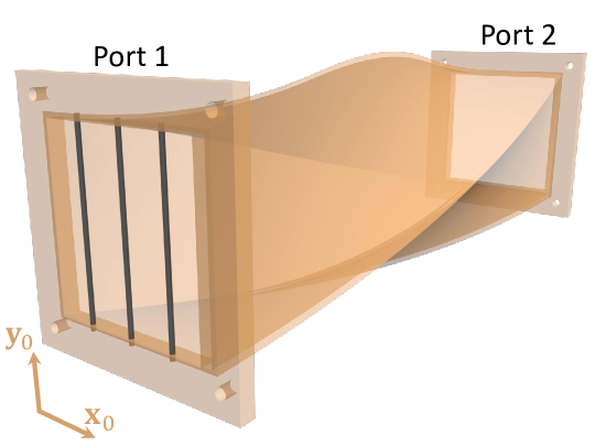
Figure 23: Twisted square-cross-section waveguide. The walls are depicted as semi-transparent to show that there is no polarization filter at the back end of the waveguide.

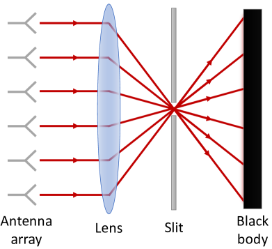
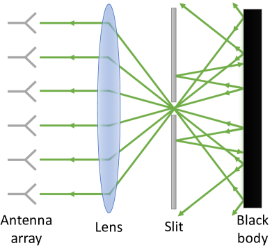
Figure 24: Asymmetric transmission in a reciprocal system formed by a perfectly conducting screen with a slit and a focusing lens.

Another simple example, illustrating the asymmetric transmission in a reciprocal system, is a lens in front of a perfectly conducting plane screen which has a small hole at its center (see Fig. 24). The lens can focus the electromagnetic energy at the location of the hole when an incident plane wave is illuminating the lens from the left, and the power will be effectively transported across the screen. In Refs. [262, 90] transmission through the lens–screen system was analysed when there were two identical antennas at the two sides of the system. Here we assume that on the left there is a directive array antenna, while on the right there is a black body. Now, it may appear from the first sight that such a system breaks reciprocity and allows transmission only from the left to the right. Indeed, when the source is the antenna, the plane wave incident on the lens will be focused onto the hole on the slit and completely absorbed by the black body (see Fig. 24). However, in the “reverse process”, the black body (effectively, it is an antenna) will radiate in all directions in a reciprocal way as shown in Fig. 24. Thus, in the reciprocal scenario there will be exactly equal power which will pass over the hole via obliquely propagating waves and received by the antenna. In particular, this conclusion means that this “asymmetrically transmitting” device cannot break the symmetry of thermal flux exchange between hot bodies on the opposite sides of the screen. It is also important to understand that if we replace the positions of the antennas, moving the directive antenna array to the right and the omnidirectional black body to the left, the power transmission will be very different from the original case. There is no contradiction with the reciprocity theorem because in this thought experiment we change the system, not only flip the positions of sources. Referring to Fig. 9, such test would be equivalent to replacing the positions of the dipole and loop antennas in addition to the positions of external sources.

It is also important to keep in mind fundamental restrictions on achievable nonreciprocal effects which come from the energy conservation principle and other fundamental physical laws. For instance, all resonators must to some extend allow coupling to outside (lossy) world just to allow excitation of fields inside the resonator. This imposes a fundamental limit on the quality factor defined by the internal resistance of the source. It would be most desirable to isolate a resonator from the sources inserting a nonreciprocal device (isolator) at the entry port [175]. However, as discussed above, ideal isolators cannot reflect energy into the resonator. Instead, they absorb it inside the isolator, meaning that the loaded quality factor of the resonator does not change if one tries to isolate the resonator from the exterior using a nonreciprocal device.

It is convenient to classify different systems providing asymmetric transmission into three basic types. This classification can be made using the scattering matrix representation given in (72). Consider a two-port system where there are two possible modes in each port (alternatively, such system can be called a four-port system). These two modes can have different polarizations or different field distributions. The scattering matrix in the general form is given by

$$\overline{\overline{S}}=\begin{pmatrix}\displaystyle S_{11}^{xx}&S_{11}^{xy}&S_{12}^{xx}&S_{12}^{xy}\vspace{1.5mm}\\ S_{11}^{yx}&S_{11}^{yy}&S_{12}^{yx}&S_{12}^{yy}\vspace{1.5mm}\\ S_{21}^{xx}&S_{21}^{xy}&S_{22}^{xx}&S_{22}^{xy}\vspace{1.5mm}\\ S_{21}^{yx}&S_{21}^{yy}&S_{22}^{yx}&S_{22}^{yy}\\ \end{pmatrix},$$ (123)

where subscripts $i,j$ denote the port number and superscripts $x,y$ denote the mode number. According to (74), for reciprocal systems the scattering matrix is symmetry $\overline{\overline{S}}=\overline{\overline{S}}^{T}$. Nevertheless, even with symmetric matrix, we can achieve peculiar scenarios of asymmetric transmission of three different types.

1. Asymmetric wave conversion characterized by $S_{12}^{yx}\neq S_{21}^{yx}$. See multiple examples of asymmetric conversion for linear and circular polarized waves [263, 264, 265, 258, 266, 267]. The waveguide in Fig. 23 also corresponds to this type (here $S_{21}^{yx}=S_{12}^{xy}$, which is in agreement with the reciprocity condition $\overline{\overline{S}}=\overline{\overline{S}}^{T}$).

2. Asymmetric transmission characterized by $S_{12}^{yx}\neq S_{21}^{xx}$. See the characteristic example of asymmetric propagation of waves with different field profiles [268, 257].

3. Unidirectional reflection characterized by $S_{11}^{xx}\neq S_{22}^{xx}$. The examples of this type include metasurfaces with asymmetric reflection properties [269, 270, 271], asymmetric diffraction gratings [272], and systems with parity-time symmetry [273].

We stress that all the works belonging to these three types correspond to reciprocal systems.

Systems with parity-time (PT) symmetry deserve a separate discussion. In such systems, the Hamiltonian is non-Hermitian, while it has an entirely real energy spectrum (see great reviews [274, 275] for optical PT symmetry). In other words, waves propagating in such systems have real propagation constants and oscillations have real frequencies. In the optical realm, a non-Hermitian Hamiltonian corresponds to a complex refractive index distribution, i.e. PT-symmetric system must have spatially alternating regions of loss and gain ${n}(x)={n}^{\ast}(-x)$, where $x$ is the coordinate. Thus, under parity (space) inversion, the lossy regions are interchanged by those with gain. Additional time reversal flips these regions again, returning to the original system. Therefore, a PT-symmetric system does not change under simultaneous space and time inversions. Importantly, the reciprocity theorem also applies to PT-symmetric systems [257, 88]. Although asymmetric reflection was demonstrated for the PT-symmetric structures ($S_{11}$ can be zero, while $S_{22}$ can have amplitude larger than unity due to the active regions), they all exhibit reciprocal transmission [273]. The only exceptions are PT-symmetric systems incorporating nonlinear [43, 40] or time-modulated components [276].

IX Conclusions

In this tutorial paper, we have attempted to provide an intuitive and concrete introduction to the concept of electromagnetic reciprocity. Since reciprocity is closely related to the time-reversal operation, we first elaborated on the conventional definition and the essense of the latter. Based on the fundamental works by Casimir, Onsager, and Sachs, we demonstrated how motion reversal with correct microscopic initial conditions results in the conventional mathematical form $t\rightarrow-t$ of the time reversal operation. Since, strictly speaking, almost all physical laws are time-reversal symmetric, it is justifiable to introduce an alternative notion of restricted time reversal. It was shown that restricted time reversal holds only in pointwise reciprocal systems, which makes these two concepts equivalent for electromagnetic systems.

Based on the microscopic time reversibility (same as time reversal defined in physics literature) and three other assumptions, a comprehensive derivation of the Onsager reciprocal relations was given, and its application to several physical processes was demonstrated. We showed that, using these fundamental relations, one can derive the reciprocity theorem proposed by Lorentz in 1896. Employment of this theorem was presented for different types of electromagnetic systems. Following Casimir’s extension of the Onsager relations, we expressed the universal restrictions imposed on nonreciprocal systems due to the microscopic reversibility. Role and meaning of reciprocity in systems characterized as multi-port networks were covered.

Next, we indicated different routes to break reciprocity in electromagnetic systems, subsequently discussing the three most common ones in detail: Materials with an external field bias, nonlinear systems, and time-varying composites. Regarding the first route, properties of multiple materials biased by magnetic field were compared for applications in different parts of the frequency spectrum. We explained the operation principles of several most important nonreciprocal components. Furthermore, space- and time-symmetry considerations were examined with the application to material tensors. A general classification of linear time-invariant media based on these considerations was presented. Building upon this classification, we were able to relate seemingly irrelevant electromagnetic effects and even envision novel ones in artificial composites. Finally, we discussed about several systems which were erroneously referred to in the literature as nonreciprocal.

Acknowledgments

This work was supported in part by the Finnish Foundation for Technology Promotion, the Academy of Finland (project 287894), Nokia Foundation (project 201920030), and by the U.S. Air Force Office of Scientific Research MURI project (Grant No. FA9550-18-1-0379). The authors thank Mr. Cheng Guo, Dr. Momchil Minkov, Prof. Steven G. Johnson, and Dr. Adi Pick for useful comments and discussions about the manuscript.

References

- [1] A. K. Zvezdin and V. A. Kotov, Modern Magnetooptics and Magnetooptical Materials. CRC Press, Jan. 1997.
- [2] D. M. Pozar, Microwave Engineering. John Wiley & Sons, 2012.
- [3] E. Bloch, “US patent 720877, ”One way mirror”,” Feb. 1903.
- [4] G. G. Stokes, “On the perfect blackness of the central spot in Newton’s rings, and on the verification of Fresnel’s formulae for the intensities of reflected and refracted rays,” Cambridge and Dublin Mathematical Journal, vol. 4, pp. 1–14, 1849.
- [5] H. v. Helmholtz, Handbuch der physiologischen Optik, vol. 1. Leipzig: L. Voss, 1856.
- [6] W. Thomson Proc. Roy. Soc. Edinburgh, vol. 3, p. 123, 1854.
- [7] G. Kirchhoff, “I. On the relation between the radiating and absorbing powers of different bodies for light and heat,” The London, Edinburgh, and Dublin Philosophical Magazine and Journal of Science, vol. 20, no. 130, pp. 1–21, 1860.
- [8] W. S. Rayleigh, Treatise on Sound, Vol. II. London: McMillan, 1878.
- [9] H. A. Lorentz, “The theorem of Poynting concerning the energy in the electromagnetic field and two general propositions concerning the propagation of light,” Amsterdammer Akademie der Wetenschappen, vol. 4, p. 176, 1896.
- [10] L. Onsager, “Reciprocal relations in irreversible processes. I.,” Physical Review, vol. 37, pp. 405–426, Feb. 1931.
- [11] L. Onsager, “Reciprocal relations in irreversible processes. II.,” Physical Review, vol. 38, pp. 2265–2279, Dec. 1931.
- [12] H. B. G. Casimir, “On Onsager’s principle of microscopic reversibility,” Reviews of Modern Physics, vol. 17, pp. 343–350, Apr. 1945.
- [13] J. Smit and H. P. J. Wijn, Ferrites: physical properties of ferrimagnetic oxides in relation to their technical applications. Eindhoven: Philips, 1959.
- [14] B. Lax and K. J. Button, Microwave ferrites and ferrimagnetics. Lincoln Laboratory publications, New York, NY: McGraw-Hill, 1962.
- [15] L. D. Landau, E. M. Lifshits, and L. P. Pitaevskii, Electrodynamics of Continuous Media, vol. 8. Oxford: Pergamon press, 2nd ed., 1984.
- [16] G. P. Rodrigue, “A generation of microwave ferrite devices,” Proceedings of the IEEE, vol. 76, pp. 121–137, Feb. 1988.
- [17] A. G. Gurevich and G. A. Melkov, Magnetization Oscillations and Waves. CRC Press, Sept. 1996.
- [18] J. D. Adam, L. E. Davis, G. F. Dionne, E. F. Schloemann, and S. N. Stitzer, “Ferrite devices and materials,” IEEE Transactions on Microwave Theory and Techniques, vol. 50, pp. 721–737, Mar. 2002.
- [19] A. Ishimaru, Electromagnetic Wave Propagation, Radiation, and Scattering: From Fundamentals to Applications. John Wiley & Sons, Sept. 2017.
- [20] N. W. Ashcroft and N. D. Mermin, Solid State Physics. Holt, Rinehart and Winston, 1976.
- [21] M. D. Tocci, M. J. Bloemer, M. Scalora, J. P. Dowling, and C. M. Bowden, “Thin–film nonlinear optical diode,” Applied Physics Letters, vol. 66, pp. 2324–2326, May 1995.
- [22] K. Gallo and G. Assanto, “All-optical diode based on second-harmonic generation in an asymmetric waveguide,” JOSA B, vol. 16, pp. 267–269, Feb. 1999.
- [23] K. Gallo, G. Assanto, K. R. Parameswaran, and M. M. Fejer, “All-optical diode in a periodically poled lithium niobate waveguide,” Applied Physics Letters, vol. 79, no. 3, pp. 314–316, 2001.
- [24] H. Zhou, K.-F. Zhou, W. Hu, Q. Guo, S. Lan, X.-S. Lin, and A. Venu Gopal, “All-optical diodes based on photonic crystal molecules consisting of nonlinear defect pairs,” Journal of Applied Physics, vol. 99, no. 12, p. 123111, 2006.
- [25] X.-S. Lin, J.-H. Yan, L.-J. Wu, and S. Lan, “High transmission contrast for single resonator based all-optical diodes with pump-assisting,” Opt. Express, vol. 16, pp. 20949–20954, Dec 2008.
- [26] S. Manipatruni, J. T. Robinson, and M. Lipson, “Optical nonreciprocity in optomechanical structures,” Phys. Rev. Lett., vol. 102, p. 213903, May 2009.
- [27] D. Roy, “Few-photon optical diode,” Phys. Rev. B, vol. 81, p. 155117, Apr 2010.
- [28] A. E. Miroshnichenko, E. Brasselet, and Y. S. Kivshar, “Reversible optical nonreciprocity in periodic structures with liquid crystals,” Applied Physics Letters, vol. 96, p. 063302, Feb. 2010.
- [29] S. Trendafilov, V. Khudik, M. Tokman, and G. Shvets, “Hamiltonian description of non-reciprocal light propagation in nonlinear chiral fibers,” Physica B: Condensed Matter, vol. 405, pp. 3003–3006, July 2010.
- [30] S. V. Zhukovsky and A. G. Smirnov, “All-optical diode action in asymmetric nonlinear photonic multilayers with perfect transmission resonances,” Phys. Rev. A, vol. 83, p. 023818, Feb 2011.
- [31] S. Lepri and G. Casati, “Asymmetric wave propagation in nonlinear systems,” Physical Review Letters, vol. 106, p. 164101, Apr. 2011.
- [32] I. V. Shadrivov, V. A. Fedotov, D. A. Powell, Y. S. Kivshar, and N. I. Zheludev, “Electromagnetic wave analogue of an electronic diode,” New Journal of Physics, vol. 13, p. 033025, March 2011.
- [33] Y. Fan, J. Han, Z. Wei, C. Wu, Y. Cao, X. Yu, and H. Li, “Subwavelength electromagnetic diode: One-way response of cascading nonlinear meta-atoms,” Applied Physics Letters, vol. 98, p. 151903, Apr. 2011.
- [34] V. Grigoriev and F. Biancalana, “Nonreciprocal switching thresholds in coupled nonlinear microcavities,” Opt. Lett., vol. 36, pp. 2131–2133, Jun 2011.
- [35] L. Fan, J. Wang, L. T. Varghese, H. Shen, B. Niu, Y. Xuan, A. M. Weiner, and M. Qi, “An all-silicon passive optical diode,” Science, vol. 335, pp. 447–450, Jan. 2012.
- [36] W. Ding, B. Luk’yanchuk, and C.-W. Qiu, “Ultrahigh-contrast-ratio silicon Fano diode,” Phys. Rev. A, vol. 85, p. 025806, Feb 2012.
- [37] B. Anand, R. Podila, K. Lingam, S. R. Krishnan, S. S. S. Sai, R. Philip, and A. M. Rao, “Optical diode action from axially asymmetric nonlinearity in an all-carbon solid-state device,” Nano Letters, vol. 13, pp. 5771–5776, nov 2013.
- [38] L. Fan, L. T. Varghese, J. Wang, Y. Xuan, A. M. Weiner, and M. Qi, “Silicon optical diode with 40 dB nonreciprocal transmission,” Opt. Lett., vol. 38, pp. 1259–1261, Apr 2013.
- [39] D. Roy, “Cascaded two-photon nonlinearity in a one-dimensional waveguide with multiple two-level emitters,” Scientific Reports, vol. 3, pp. 1–5, Aug. 2013.
- [40] L. Chang, X. Jiang, S. Hua, C. Yang, J. Wen, L. Jiang, G. Li, G. Wang, and M. Xiao, “Parity-time symmetry and variable optical isolation in active-passive-coupled microresonators,” Nature Photonics, vol. 8, pp. 524–529, July 2014.
- [41] Y. Xu and A. E. Miroshnichenko, “Reconfigurable nonreciprocity with a nonlinear Fano diode,” Phys. Rev. B, vol. 89, p. 134306, Apr 2014.
- [42] F. Nazari, N. Bender, H. Ramezani, M. K. Moravvej-Farshi, D. N. Christodoulides, and T. Kottos, “Optical isolation via PT-symmetric nonlinear Fano resonances,” Optics Express, vol. 22, pp. 9574–9584, Apr. 2014.
- [43] B. Peng, Ş. K. Özdemir, F. Lei, F. Monifi, M. Gianfreda, G. L. Long, S. Fan, F. Nori, C. M. Bender, and L. Yang, “Parity–time-symmetric whispering-gallery microcavities,” Nature Physics, vol. 10, pp. 394–398, apr 2014.
- [44] Y. Shi, Z. Yu, and S. Fan, “Limitations of nonlinear optical isolators due to dynamic reciprocity,” Nature Photonics, vol. 9, pp. 388–392, June 2015.
- [45] Y. Yu, Y. Chen, H. Hu, W. Xue, K. Yvind, and J. Mork, “Nonreciprocal transmission in a nonlinear photonic-crystal fano structure with broken symmetry,” Laser & Photonics Reviews, vol. 9, no. 2, pp. 241–247, 2015.
- [46] A. M. Mahmoud, A. R. Davoyan, and N. Engheta, “All-passive nonreciprocal metastructure,” Nature Communications, vol. 6, p. 8359, Sept. 2015.
- [47] D. L. Sounas and A. Alù, “Time-reversal symmetry bounds on the electromagnetic response of asymmetric structures,” Physical Review Letters, vol. 118, p. 154302, Apr. 2017.
- [48] D. Roy, “Critical features of nonlinear optical isolators for improved nonreciprocity,” Physical Review A, vol. 96, p. 033838, Sept. 2017.
- [49] P. Aleahmad, M. Khajavikhan, D. Christodoulides, and P. LiKamWa, “Integrated multi-port circulators for unidirectional optical information transport,” Scientific Reports, vol. 7, May 2017.
- [50] L. D. Bino, J. M. Silver, M. T. M. Woodley, S. L. Stebbings, X. Zhao, and P. Del’Haye, “Microresonator isolators and circulators based on the intrinsic nonreciprocity of the Kerr effect,” Optica, vol. 5, pp. 279–282, Mar. 2018.
- [51] A. Rosario Hamann, C. Müller, M. Jerger, M. Zanner, J. Combes, M. Pletyukhov, M. Weides, T. M. Stace, and A. Fedorov, “Nonreciprocity realized with quantum nonlinearity,” Physical Review Letters, vol. 121, p. 123601, Sept. 2018.
- [52] D. L. Sounas, J. Soric, and A. Alù, “Broadband passive isolators based on coupled nonlinear resonances,” Nature Electronics, vol. 1, p. 113, Feb. 2018.
- [53] D. L. Sounas and A. Alù, “Nonreciprocity based on nonlinear resonances,” IEEE Antennas and Wireless Propagation Letters, vol. 17, pp. 1958–1962, Nov. 2018.
- [54] T. Kodera, D. L. Sounas, and C. Caloz, “Artificial Faraday rotation using a ring metamaterial structure without static magnetic field,” Applied Physics Letters, vol. 99, no. 3, p. 031114, 2011.
- [55] T. Kodera, D. L. Sounas, and C. Caloz, “Nonreciprocal magnetless CRLH leaky-wave antenna based on a ring metamaterial structure,” IEEE Antennas and Wireless Propagation Letters, vol. 10, pp. 1551–1554, 2011.
- [56] D. L. Sounas, T. Kodera, and C. Caloz, “Electromagnetic modeling of a magnetless nonreciprocal gyrotropic metasurface,” IEEE Transactions on Antennas and Propagation, vol. 61, pp. 221–231, Jan. 2013.
- [57] T. Kodera and C. Caloz, “Unidirectional loop metamaterials (ULM) as magnetless artificial ferrimagnetic materials: principles and applications,” IEEE Antennas and Wireless Propagation Letters, vol. 17, pp. 1943–1947, Nov. 2018.
- [58] A. L. Cullen, “A travelling-wave parametric amplifier,” Nature, vol. 181, p. 332, Feb. 1958.
- [59] J. C. Slater, “Interaction of waves in crystals,” Reviews of Modern Physics, vol. 30, pp. 197–222, Jan. 1958.
- [60] A. Fettweis, “Steady-state analysis of circuits containing a periodically-operated switch,” IRE Transactions on Circuit Theory, vol. 6, pp. 252–260, Sept. 1959.
- [61] A. K. Kamal, “A parametric device as a nonreciprocal element,” Proceedings of the IRE, vol. 48, pp. 1424–1430, Aug. 1960.
- [62] M. R. Currie and R. W. Gould, “Coupled-cavity traveling-wave parametric amplifiers: Part I-Analysis,” Proceedings of the IRE, vol. 48, pp. 1960–1973, Dec. 1960.
- [63] J.-C. Simon, “Action of a progressive disturbance on a guided electromagnetic wave,” IRE Transactions on Microwave Theory and Techniques, vol. 8, pp. 18–29, Jan. 1960.
- [64] J. R. Macdonald and D. E. Edmondson, “Exact solution of a time-varying capacitance problem,” Proceedings of the IRE, vol. 49, pp. 453–466, Feb. 1961.
- [65] A. Oliner and A. Hessel, “Wave propagation in a medium with a progressive sinusoidal disturbance,” IRE Transactions on Microwave Theory and Techniques, vol. 9, pp. 337–343, July 1961.
- [66] B. D. O. Anderson and R. W. Newcomb, “On reciprocity and time-variable networks,” Proceedings of the IEEE, vol. 53, pp. 1674–1674, Oct. 1965.
- [67] D. Holberg and K. Kunz, “Parametric properties of fields in a slab of time-varying permittivity,” IEEE Transactions on Antennas and Propagation, vol. 14, pp. 183–194, Mar. 1966.
- [68] Z. Yu and S. Fan, “Complete optical isolation created by indirect interband photonic transitions,” Nature Photonics, vol. 3, pp. 91–94, Feb. 2009.
- [69] Z. Yu and S. Fan, “Optical isolation based on nonreciprocal phase shift induced by interband photonic transitions,” Applied Physics Letters, vol. 94, p. 171116, Apr. 2009.
- [70] M. S. Kang, A. Butsch, and P. S. J. Russell, “Reconfigurable light-driven opto-acoustic isolators in photonic crystal fibre,” Nature Photonics, vol. 5, pp. 549–553, Sept. 2011.
- [71] H. Lira, Z. Yu, S. Fan, and M. Lipson, “Electrically driven nonreciprocity induced by interband photonic transition on a silicon chip,” Physical Review Letters, vol. 109, p. 033901, July 2012.
- [72] K. Fang, Z. Yu, and S. Fan, “Photonic Aharonov-Bohm effect based on dynamic modulation,” Physical Review Letters, vol. 108, p. 153901, Apr. 2012.
- [73] K. Fang, Z. Yu, and S. Fan, “Realizing effective magnetic field for photons by controlling the phase of dynamic modulation,” Nature Photonics, vol. 6, pp. 782–787, Nov. 2012.
- [74] D.-W. Wang, H.-T. Zhou, M.-J. Guo, J.-X. Zhang, J. Evers, and S.-Y. Zhu, “Optical diode made from a moving photonic crystal,” Physical Review Letters, vol. 110, p. 093901, Feb. 2013.
- [75] S. A. R. Horsley, J.-H. Wu, M. Artoni, and G. C. La Rocca, “Optical nonreciprocity of cold atom Bragg mirrors in motion,” Physical Review Letters, vol. 110, p. 223602, May 2013.
- [76] D. L. Sounas, C. Caloz, and A. Alù, “Giant non-reciprocity at the subwavelength scale using angular momentum-biased metamaterials,” Nature Communications, vol. 4, p. 2407, Sept. 2013.
- [77] K. Fang and S. Fan, “Controlling the flow of light using the inhomogeneous effective gauge field that emerges from dynamic modulation,” Physical Review Letters, vol. 111, p. 203901, Nov. 2013.
- [78] S. Qin, Q. Xu, and Y. E. Wang, “Nonreciprocal components with distributedly modulated capacitors,” IEEE Transactions on Microwave Theory and Techniques, vol. 62, pp. 2260–2272, Oct. 2014.
- [79] N. A. Estep, D. L. Sounas, J. Soric, and A. Alù, “Magnetic-free non-reciprocity and isolation based on parametrically modulated coupled-resonator loops,” Nature Physics, vol. 10, pp. 923–927, Dec. 2014.
- [80] L. D. Tzuang, K. Fang, P. Nussenzveig, S. Fan, and M. Lipson, “Non-reciprocal phase shift induced by an effective magnetic flux for light,” Nature Photonics, vol. 8, pp. 701–705, Sept. 2014.
- [81] Q. Lin and S. Fan, “Light guiding by effective gauge field for photons,” Physical Review X, vol. 4, p. 031031, Aug. 2014.
- [82] A. Shaltout, A. Kildishev, and V. Shalaev, “Time-varying metasurfaces and Lorentz non-reciprocity,” Optical Materials Express, vol. 5, pp. 2459–2467, Nov. 2015.
- [83] Y. Hadad, D. Sounas, and A. Alù, “Space-time gradient metasurfaces,” Physical Review B, vol. 92, no. 10, p. 100304, 2015.
- [84] Y. Hadad, J. C. Soric, and A. Alù, “Breaking temporal symmetries for emission and absorption,” Proceedings of the National Academy of Sciences, p. 201517363, Mar. 2016.
- [85] D. Correas-Serrano, J. S. Gomez-Diaz, D. L. Sounas, Y. Hadad, A. Alvarez-Melcon, and A. Alù, “Nonreciprocal graphene devices and antennas based on spatiotemporal modulation,” IEEE Antennas and Wireless Propagation Letters, vol. 15, pp. 1529–1532, 2016.
- [86] S. Taravati and C. Caloz, “Mixer-duplexer-antenna leaky-wave system based on periodic space-time modulation,” IEEE Transactions on Antennas and Propagation, vol. 65, pp. 442–452, Feb. 2017.
- [87] R. J. Potton, “Reciprocity in optics,” Reports on Progress in Physics, vol. 67, pp. 717–754, Apr. 2004.
- [88] D. Jalas, A. Petrov, M. Eich, W. Freude, S. Fan, Z. Yu, R. Baets, M. Popović, A. Melloni, J. D. Joannopoulos, M. Vanwolleghem, C. R. Doerr, and H. Renner, “What is – and what is not – an optical isolator,” Nature Photonics, vol. 7, pp. 579–582, July 2013.
- [89] D. L. Sounas and A. Andrea, “Non-reciprocal photonics based on time modulation,” Nature Photonics, vol. 11, pp. 774–783, 2017.
- [90] C. Caloz, A. Alù, S. Tretyakov, D. Sounas, K. Achouri, and Z.-L. Deck-Léger, “Electromagnetic nonreciprocity,” Physical Review Applied, vol. 10, p. 047001, Oct. 2018.
- [91] S. Fan, Y. Shi, and Q. Lin, “Nonreciprocal photonics without magneto-optics,” IEEE Antennas and Wireless Propagation Letters, vol. 17, pp. 1948–1952, Nov. 2018.
- [92] C. Caloz and Z.-L. Deck-Léger, “Spacetime metamaterials, Part I: General concepts,” IEEE Transactions on Antennas and Propagation, pp. 1–1, 2019.
- [93] C. Caloz and Z.-L. Deck-Léger, “Spacetime metamaterials, Part II: Theory and applications,” IEEE Transactions on Antennas and Propagation, pp. 1–1, 2019.
- [94] X. Guo, Y. Ding, Y. Duan, and X. Ni, “Nonreciprocal metasurface with space–time phase modulation,” Light: Science & Applications, vol. 8, p. 123, Dec. 2019.
- [95] L. Zhang, X. Q. Chen, R. W. Shao, J. Y. Dai, Q. Cheng, G. Castaldi, V. Galdi, and T. J. Cui, “Breaking reciprocity with space-time-coding digital metasurfaces,” Advanced Materials, vol. 31, no. 41, p. 1904069, 2019.
- [96] A. Nagulu, N. Reiskarimian, and H. Krishnaswamy, “Non-reciprocal electronics based on temporal modulation,” Nature Electronics, vol. 3, pp. 241–250, May 2020.
- [97] I. A. D. Williamson, M. Minkov, A. Dutt, J. Wang, A. Y. Song, and S. Fan, “Breaking reciprocity in integrated photonic devices through dynamic modulation,” arXiv:2002.04754v1, Feb. 2020.
- [98] D. K. Cheng, Field and wave electromagnetics. Addison Wesley, 1983.
- [99] R. G. Sachs, “Can the direction of flow of time be determined?,” Science, vol. 140, no. 3573, pp. 1284–1290, 1963.
- [100] R. G. Sachs, The Physics of Time Reversal. University of Chicago Press, Oct. 1987.
- [101] H. Casimir, “Reciprocity theorems and irreversible processes,” Proceedings of the IEEE, vol. 51, pp. 1570–1573, Nov. 1963.
- [102] R. G. Sachs, “Time reversal,” Science, vol. 176, no. 4035, pp. 587–597, 1972.
- [103] J. A. G. Roberts and G. R. W. Quispel, “Chaos and time-reversal symmetry. Order and chaos in reversible dynamical systems,” Physics Reports, vol. 216, pp. 63–177, July 1992.
- [104] M. G. Silveirinha, “Hidden time-reversal symmetry in dissipative reciprocal systems,” Optics Express, vol. 27, pp. 14328–14337, May 2019.
- [105] L. D. Barron, Molecular Light Scattering and Optical Activity. Cambridge University Press, Oct. 2009.
- [106] E. J. Post, Formal Structure of Electromagnetics. Amsterdam: North-Holland Publishing Company, 1962.
- [107] I. V. Lindell, Methods for Electromagnetic Field Analysis. Oxford: Clarendon Press, 1992.
- [108] J. D. Jackson, Classical Electrodynamics. John Wiley Sons, Inc., 1999.
- [109] J. North, “Two views on time reversal,” Philosophy of Science, vol. 75, no. 2, pp. 201–223, 2008.
- [110] E. J. Post, “The logic of time reversal,” Foundations of Physics, vol. 9, pp. 129–161, Feb. 1979.
- [111] P. Horwich, Asymmetries in Time: Problems in the Philosophy of Science. Bradford Books, 1989.
- [112] D. Z. Albert, Time and Chance. Harvard University Press, 2000.
- [113] D. B. Malament, “On the time reversal invariance of classical electromagnetic theory,” Studies in History and Philosophy of Science Part B: Studies in History and Philosophy of Modern Physics, vol. 35, pp. 295–315, June 2004.
- [114] J. Loschmidt, “Uber das warmegleichgewicht eines systems von korpern mit rucksicht auf die schwere,” Sitzungsber. Kais. Akad. Wiss. Wien, Math. Naturwiss., vol. 73, pp. 128–142, 1876.
- [115] J. Schwinger, “The theory of quantized fields. I,” Physical Review, vol. 82, pp. 914–927, June 1951.
- [116] A. Serdyukov, I. Semchenko, S. Tretyakov, and A. Sihvola, Electromagnetics of Bi-Anisotropic Materials - Theory and Application, vol. 11. Amsterdam: Gordon and Breach Science Publishers, 2001.
- [117] C. Altman and K. Suchy, “Generalization of an eigemnode scattering theorem,” Journal of Electromagnetic Waves and Applications, vol. 5, pp. 685–700, Jan. 1991.
- [118] V. A. Dmitriev, “Space-time reversal symmetry properties of electromagnetic Green’s tensors for complex and bianisotropic media,” Progress In Electromagnetics Research, vol. 48, pp. 145–184, 2004.
- [119] C. Altman and K. Suchy, Reciprocity, Spatial Mapping and Time Reversal in Electromagnetics. Springer Science & Business Media, July 2011.
- [120] L. D. Landau and E. M. Lifshitz, Statistical Physics, part 1 (Course of Theoretical Physics). Oxford: Elsevier, 1980.
- [121] H. B. Callen and T. A. Welton, “Irreversibility and generalized noise,” Physical Review, vol. 83, pp. 34–40, July 1951.
- [122] D. G. Miller, “Thermodynamics of irreversible processes. The experimental verification of the onsager reciprocal relations.,” Chemical Reviews, vol. 60, pp. 15–37, Feb. 1960.
- [123] L. Novotny and B. Hecht, Principles of Nano-Optics. New York: Cambridge university press, 2006.
- [124] W. L. Stutzman and G. A. Thiele, Antenna Theory and Design. John Wiley & Sons, 1998.
- [125] V. S. Asadchy, A. Díaz-Rubio, and S. A. Tretyakov, “Bianisotropic metasurfaces: Physics and applications,” Nanophotonics, vol. 7, no. 6, pp. 1069–1094, 2018.
- [126] G. T. Rado, “Reciprocity relations for susceptibilities and fields in magnetoelectric antiferromagnets,” Physical Review B, vol. 8, pp. 5239–5242, Dec. 1973.
- [127] B. V. Bokut’ and A. N. Serdyukov, “Phenomenological theory of absorbing optically-active media,” Optika i Spektroskopiya (in Russian), vol. 37, no. 1, pp. 120–124, 1974. http://elib.gsu.by/handle/123456789/7504.
- [128] J. A. Kong, Electromagnetic Wave Theory. New York: Wiley, 1986.
- [129] V. H. Rumsey, “Reaction concept in electromagnetic theory,” Physical Review, vol. 94, pp. 1483–1491, June 1954.
- [130] J. R. Schulenberger and C. H. Wilcox, “The limiting absorption principle and spectral theory for steady-state wave propagation in inhomogeneous anisotropic media,” Archive for Rational Mechanics and Analysis, vol. 41, pp. 46–65, Jan. 1971.
- [131] A. Kirsch and A. Lechleiter, “The limiting absorption principle and a radiation condition for the scattering by a periodic layer,” SIAM Journal on Mathematical Analysis, vol. 50, pp. 2536–2565, Jan. 2018.
- [132] V. Asadchy, Spatially dispersive metasurfaces. PhD thesis, Aalto University, 2017.
- [133] C. Caloz and S. Tretyakov, “Nonreciprocal metamaterials: A global perspective,” in 2016 10th International Congress on Advanced Electromagnetic Materials in Microwaves and Optics (Metamaterials’ 2016), pp. 76–78, Sept. 2016.
- [134] A. Shlivinski, “Time-domain transfer coupled response of antennas–reciprocity theorem approach,” IEEE Transactions on Antennas and Propagation, vol. 65, pp. 1714–1727, April 2017.
- [135] B. Cheo, “A reciprocity theorem for electromagnetic fields with general time dependence,” IEEE Transactions on Antennas and Propagation, vol. 13, pp. 278–284, March 1965.
- [136] L. P. Pitaevskii, “Electric forces in a transparent dispersive medium,” Soviet Physics (JETP), vol. 12, no. 5, pp. 1008–1013, 1961.
- [137] N. Marcuvitz and M. I. o. T. R. Laboratory, Waveguide Handbook. IET, 1951.
- [138] V. S. Asadchy, D.-R. A., S. N. Tcvetkova, D.-H. Kwon, A. Elsakka, M. Albooyeh, and S. A. Tretyakov, “Flat engineered multichannel reflectors,” Phys. Rev. X, vol. 7, no. 3, p. 031046, 2017.
- [139] B. D. H. Tellegen, “The gyrator, a new electric network element,” Philips Research Reports, vol. 3, no. 2, pp. 81–101, 1948.
- [140] Y. Demirel, “3 - Fundamentals of nonequilibrium thermodynamics,” in Nonequilibrium Thermodynamics (Second Edition) (Y. Demirel, ed.), pp. 97–154, Amsterdam: Elsevier Science B.V., Jan. 2007.
- [141] Z. Wang, Z. Wang, J. Wang, B. Zhang, J. Huangfu, J. D. Joannopoulos, M. Soljačić, and L. Ran, “Gyrotropic response in the absence of a bias field,” Proceedings of the National Academy of Sciences, vol. 109, no. 33, pp. 13194–13197, 2012.
- [142] S. Taravati, B. A. Khan, S. Gupta, K. Achouri, and C. Caloz, “Nonreciprocal nongyrotropic magnetless metasurface,” IEEE Transactions on Antennas and Propagation, vol. 65, pp. 3589–3597, July 2017.
- [143] A. Crisanti and F. Ritort, “Violation of the fluctuation-dissipation theorem in glassy systems: Basic notions and the numerical evidence,” Journal of Physics A: Mathematical and General, vol. 36, pp. R181–R290, May 2003.
- [144] M. Faraday, “On the magnetization of light and the illumination of magnetic lines of force,” Philosophical Transactions of the Royal Society of London, vol. 136, pp. 1–20, 1846.
- [145] K. E. Oughstun and R. A. Albanese, “Magnetic field contribution to the Lorentz model,” JOSA A, vol. 23, pp. 1751–1756, July 2006.
- [146] W. Kleemann, “Magneto-optical Materials,” in Handbook of Magnetism and Advanced Magnetic Materials, American Cancer Society, 2007.
- [147] T. Haider, “A review of magneto-optic effects and its application,” International Journal of Electromagnetics and Applications, vol. 7, no. 1, pp. 17–24, 2017.
- [148] J. M. D. Coey, Magnetism and Magnetic Materials. New York: Cambridge University Press, 2010.
- [149] S. Sugano and N. Kojima, Magneto-Optics. New York: Springer Science & Business Media, Mar. 2013.
- [150] J. K. LL.D, “On rotation of the plane of polarization by reflection from the pole of a magnet,” The London, Edinburgh, and Dublin Philosophical Magazine and Journal of Science, vol. 3, pp. 321–343, May 1877.
- [151] P. S. Pershan, “Nonlinear optical properties of solids: Energy considerations,” Physical Review, vol. 130, pp. 919–929, May 1963.
- [152] V. I. Belotelov and A. K. Zvezdin, “Inverse transverse magneto-optical Kerr effect,” Physical Review B, vol. 86, p. 155133, Oct. 2012.
- [153] R. Hertel, “Theory of the inverse Faraday effect in metals,” Journal of Magnetism and Magnetic Materials, vol. 303, pp. L1–L4, Aug. 2006.
- [154] H.-L. Zhang, Y.-Z. Wang, and X.-J. Chen, “A simple explanation for the inverse Faraday effect in metals,” Journal of Magnetism and Magnetic Materials, vol. 321, pp. L73–L74, Dec. 2009.
- [155] J. P. van der Ziel, P. S. Pershan, and L. D. Malmstrom, “Optically-induced magnetization resulting from the inverse Faraday effect,” Physical Review Letters, vol. 15, pp. 190–193, Aug. 1965.
- [156] A. V. Kimel, A. Kirilyuk, and T. Rasing, “Femtosecond opto-magnetism: Ultrafast laser manipulation of magnetic materials,” Laser & Photonics Reviews, vol. 1, no. 3, pp. 275–287, 2007.
- [157] A. Cotton and H. Mouton, “Sur les propriétés magnétooptiques des colloides et des liqueurs hétérogenes,” Ann Chim Phys, vol. 11, pp. 145–203, 1907.
- [158] M. v. Smoluchowski, “Handbuch der Elektrizität und des Magnetismus,” Band II, Barth-Verlag, Leipzig, 1921.
- [159] D. Polder, “On the theory of ferromagnetic resonance,” The London, Edinburgh, and Dublin Philosophical Magazine and Journal of Science, vol. 40, pp. 99–115, Jan. 1949.
- [160] C. L. Hogan, “The ferromagnetic Faraday effect at microwave frequencies and its applications: The microwave gyrator,” The Bell System Technical Journal, vol. 31, pp. 1–31, Jan. 1952.
- [161] M. Shirasaki, N. Tagaki, and T. Obokata, “Bistable optical switch using a yttrium-iron-garnet crystal with phase matching films,” Applied Physics Letters, vol. 38, pp. 833–834, June 1981.
- [162] G. Scott and D. Lacklison, “Magnetooptic properties and applications of bismuth substituted iron garnets,” IEEE Transactions on Magnetics, vol. 12, pp. 292–311, July 1976.
- [163] T. R. Johansen, D. I. Norman, and E. J. Torok, “Variation of stripe–domain spacing in a Faraday effect light deflector,” Journal of Applied Physics, vol. 42, pp. 1715–1716, Mar. 1971.
- [164] J. T. Chang, J. F. Dillon, and U. F. Gianola, “Magneto–optical variable memory based upon the properties of a transparent ferrimagnetic garnet at its compensation temperature,” Journal of Applied Physics, vol. 36, pp. 1110–1111, Mar. 1965.
- [165] C. Padula and C. Young, “Optical isolators for high-power 1.06-micron glass laser system,” IEEE Journal of Quantum Electronics, vol. 3, pp. 493–498, Nov. 1967.
- [166] K. Kobayashi and M. Seki, “Microoptic grating multiplexers and optical isolators for fiber-optic communications,” IEEE Journal of Quantum Electronics, vol. 16, pp. 11–22, Jan. 1980.
- [167] E. G. Víllora, P. Molina, M. Nakamura, K. Shimamura, T. Hatanaka, A. Funaki, and K. Naoe, “Faraday rotator properties of {Tb}[ScLu](Al)O, a highly transparent terbium-garnet for visible-infrared optical isolators,” Applied Physics Letters, vol. 99, p. 011111, July 2011.
- [168] Z. Chen, L. Yang, Y. Hang, and X. Wang, “Preparation and characterization of highly transparent Ce3+ doped terbium gallium garnet single crystal,” Optical Materials, vol. 47, pp. 39–43, Sept. 2015.
- [169] J. G. Bai, G.-Q. Lu, and T. Lin, “Magneto-optical current sensing for applications in integrated power electronics modules,” Sensors and Actuators A: Physical, vol. 109, pp. 9–16, Dec. 2003.
- [170] http://www.internationalcrystal.net/icl_may5.pdf.
- [171] L. Weller, K. S. Kleinbach, M. A. Zentile, S. Knappe, I. G. Hughes, and C. S. Adams, “Optical isolator using an atomic vapor in the hyperfine Paschen–Back regime,” Optics Letters, vol. 37, pp. 3405–3407, Aug. 2012.
- [172] J. A. Gaj, R. R. Gaa¸zka, and M. Nawrocki, “Giant exciton Faraday rotation in CdMnTe mixed crystals,” Solid State Communications, vol. 25, pp. 193–195, Jan. 1978.
- [173] W. Zhao, “Magneto-optic properties and sensing performance of garnet YbBi:YIG,” Sensors and Actuators A: Physical, vol. 89, pp. 250–254, Apr. 2001.
- [174] T. Arikawa, X. Wang, A. A. Belyanin, and J. Kono, “Giant tunable Faraday effect in a semiconductor magneto-plasma for broadband terahertz polarization optics,” Optics Express, vol. 20, pp. 19484–19492, Aug. 2012.
- [175] K. L. Tsakmakidis, L. Shen, S. A. Schulz, X. Zheng, J. Upham, X. Deng, H. Altug, A. F. Vakakis, and R. W. Boyd, “Breaking Lorentz reciprocity to overcome the time-bandwidth limit in physics and engineering,” Science, vol. 356, pp. 1260–1264, June 2017.
- [176] M. Shalaby, M. Peccianti, Y. Ozturk, and R. Morandotti, “A magnetic non-reciprocal isolator for broadband terahertz operation,” Nature Communications, vol. 4, p. 1558, Mar. 2013.
- [177] P. J. Allen, “A microwave magnetometer,” Proceedings of the IRE, vol. 41, pp. 100–104, Jan. 1953.
- [178] F. R. Prudêncio and M. G. Silveirinha, “Optical isolation of circularly polarized light with a spontaneous magnetoelectric effect,” Phys. Rev. A, vol. 93, p. 043846, Apr 2016.
- [179] N. A. Spaldin and R. Ramesh, “Advances in magnetoelectric multiferroics,” Nature Materials, vol. 18, p. 203, Mar. 2019.
- [180] A. V. Kimel, G. V. Astakhov, G. M. Schott, A. Kirilyuk, D. R. Yakovlev, G. Karczewski, W. Ossau, G. Schmidt, L. W. Molenkamp, and T. Rasing, “Picosecond dynamics of the photoinduced spin polarization in epitaxial (Ga,Mn)As films,” Physical Review Letters, vol. 92, p. 237203, June 2004.
- [181] J. R. Neal, A. J. Behan, R. M. Ibrahim, H. J. Blythe, M. Ziese, A. M. Fox, and G. A. Gehring, “Room-temperature magneto-optics of ferromagnetic transition-metal-doped ZnO thin films,” Physical Review Letters, vol. 96, p. 197208, May 2006.
- [182] C. Gould, K. Pappert, G. Schmidt, and L. W. Molenkamp, “Magnetic anisotropies and (Ga,Mn)As-based spintronic devices,” Advanced Materials, vol. 19, no. 3, pp. 323–340, 2007.
- [183] S. Vandendriessche, S. Van Cleuvenbergen, P. Willot, G. Hennrich, M. Srebro, V. K. Valev, G. Koeckelberghs, K. Clays, J. Autschbach, and T. Verbiest, “Giant Faraday rotation in mesogenic organic molecules,” Chemistry of Materials, vol. 25, pp. 1139–1143, Apr. 2013.
- [184] V. P. Gusynin, S. G. Sharapov, and J. P. Carbotte, “Magneto-optical conductivity in graphene,” Journal of Physics: Condensed Matter, vol. 19, p. 026222, Dec. 2006.
- [185] I. Crassee, J. Levallois, A. L. Walter, M. Ostler, A. Bostwick, E. Rotenberg, T. Seyller, D. van der Marel, and A. B. Kuzmenko, “Giant Faraday rotation in single- and multilayer graphene,” Nature Physics, vol. 7, pp. 48–51, Jan. 2011.
- [186] A. Shuvaev, V. Dziom, Z. D. Kvon, N. N. Mikhailov, and A. Pimenov, “Universal Faraday rotation in HgTe wells with critical thickness,” Physical Review Letters, vol. 117, p. 117401, Sept. 2016.
- [187] L. Wu, M. Salehi, N. Koirala, J. Moon, S. Oh, and N. P. Armitage, “Quantized faraday and Kerr rotation and axion electrodynamics of a 3D topological insulator,” Science, vol. 354, no. 6316, pp. 1124–1127, 2016.
- [188] V. Dziom, A. Shuvaev, A. Pimenov, G. V. Astakhov, C. Ames, K. Bendias, J. Böttcher, G. Tkachov, E. M. Hankiewicz, C. Brüne, H. Buhmann, and L. W. Molenkamp, “Observation of the universal magnetoelectric effect in a 3D topological insulator,” Nature Communications, vol. 8, p. 15197, May 2017.
- [189] B. Yan and C. Felser, “Topological materials: Weyl semimetals,” Annual Review of Condensed Matter Physics, vol. 8, pp. 337–354, Mar. 2017.
- [190] S. Kar and A. M. Jayannavar, “Weyl semimetals: Down the discovery of topological phases,” arXiv:1902.01620 [cond-mat], Feb. 2019.
- [191] J. Hofmann and S. Das Sarma, “Surface plasmon polaritons in topological Weyl semimetals,” Physical Review B, vol. 93, p. 241402, June 2016.
- [192] O. V. Kotov and Y. E. Lozovik, “Giant tunable nonreciprocity of light in Weyl semimetals,” Physical Review B, vol. 98, p. 195446, Nov. 2018.
- [193] A. M. Shuvaev, G. V. Astakhov, A. Pimenov, C. Brüne, H. Buhmann, and L. W. Molenkamp, “Giant magneto-optical Faraday effect in HgTe thin films in the terahertz spectral range,” Physical Review Letters, vol. 106, p. 107404, Mar. 2011.
- [194] V. S. Asadchy, C. Guo, B. Zhao, and S. Fan, “Sub-wavelength passive optical isolators using photonic structures based on Weyl semimetals,” Advanced Optical Materials, vol. n/a, no. n/a, p. 2000100, 2020.
- [195] Q. Du, C. Wang, Y. Zhang, Y. Zhang, T. Fakhrul, W. Zhang, C. Gonçalves, C. Blanco, K. Richardson, L. Deng, C. A. Ross, L. Bi, and J. Hu, “Monolithic on-chip magneto-optical isolator with 3 dB insertion loss and 40 dB isolation ratio,” ACS Photonics, vol. 5, pp. 5010–5016, Dec. 2018.
- [196] Y. Zhang, Q. Du, C. Wang, T. Fakhrul, S. Liu, L. Deng, D. Huang, P. Pintus, J. Bowers, C. A. Ross, J. Hu, and L. Bi, “Monolithic integration of broadband optical isolators for polarization-diverse silicon photonics,” Optica, vol. 6, pp. 473–478, Apr. 2019.
- [197] A. Figotin and I. Vitebsky, “Nonreciprocal magnetic photonic crystals,” Physical Review E, vol. 63, p. 066609, May 2001.
- [198] I. L. Lyubchanskii, N. N. Dadoenkova, M. I. Lyubchanskii, E. A. Shapovalov, and T. Rasing, “Magnetic photonic crystals,” Journal of Physics D: Applied Physics, vol. 36, pp. R277–R287, Sept. 2003.
- [199] A. B. Khanikaev, A. V. Baryshev, M. Inoue, A. B. Granovsky, and A. P. Vinogradov, “Two-dimensional magnetophotonic crystal: Exactly solvable model,” Physical Review B, vol. 72, p. 035123, July 2005.
- [200] Z. Yu, Z. Wang, and S. Fan, “One-way total reflection with one-dimensional magneto-optical photonic crystals,” Applied Physics Letters, vol. 90, p. 121133, Mar. 2007.
- [201] A. B. Khanikaev, A. V. Baryshev, A. A. Fedyanin, A. B. Granovsky, and M. Inoue, “Anomalous Faraday effect of a system with extraordinary optical transmittance,” Optics Express, vol. 15, pp. 6612–6622, May 2007.
- [202] V. I. Belotelov, D. A. Bykov, L. L. Doskolovich, A. N. Kalish, and A. K. Zvezdin, “Extraordinary transmission and giant magneto-optical transverse Kerr effect in plasmonic nanostructured films,” JOSA B, vol. 26, pp. 1594–1598, Aug. 2009.
- [203] A. B. Khanikaev, S. H. Mousavi, G. Shvets, and Y. S. Kivshar, “One-way extraordinary optical transmission and nonreciprocal spoof plasmons,” Physical Review Letters, vol. 105, p. 126804, Sept. 2010.
- [204] S. H. Mousavi, A. B. Khanikaev, J. Allen, M. Allen, and G. Shvets, “Gyromagnetically induced transparency of metasurfaces,” Physical Review Letters, vol. 112, p. 117402, Mar. 2014.
- [205] A. Christofi, Y. Kawaguchi, A. Alù, and A. B. Khanikaev, “Giant enhancement of Faraday rotation due to electromagnetically induced transparency in all-dielectric magneto-optical metasurfaces,” Optics Letters, vol. 43, pp. 1838–1841, Apr. 2018.
- [206] L. Ying, M. Zhou, X. Luo, J. Liu, and Z. Yu, “Strong magneto-optical response enabled by quantum two-level systems,” Optica, vol. 5, pp. 1156–1162, Sept. 2018.
- [207] P. M. Rinard and J. W. Calvert, “The Faraday effect and inversion symmetries,” American Journal of Physics, vol. 39, pp. 753–756, July 1971.
- [208] L. D. Barron, “Parity and optical activity,” Nature, vol. 238, p. 17, July 1972.
- [209] E. U. Condon, “Theories of optical rotatory power,” Reviews of Modern Physics, vol. 9, pp. 432–457, Oct. 1937.
- [210] A. H. Sihvola and I. V. Lindell, “Bi-isotropic constitutive relations,” Microwave and Optical Technology Letters, vol. 4, no. 8, pp. 295–297, 1991.
- [211] W. T. B. Kelvin, Baltimore Lectures on Molecular Dynamics and the Wave Theory of Light. C.J. Clay and Sons, 1904.
- [212] R. V. Jones, “Rotary ’aether drag’,” Proceedings of the Royal Society of London. A. Mathematical and Physical Sciences, vol. 349, pp. 423–439, June 1976.
- [213] V. Dmitriev, “Group theoretical approach to complex and bianisotropic media description,” The European Physical Journal - Applied Physics, vol. 6, pp. 49–55, Apr. 1999.
- [214] S. A. Tretyakov, “Nonreciprocal composite with the material relations of the transparent absorbing boundary,” Microwave and Optical Technology Letters, vol. 19, pp. 365–368, Dec. 1998.
- [215] A. D. LaForge, A. Frenzel, B. C. Pursley, T. Lin, X. Liu, J. Shi, and D. N. Basov, “Optical characterization of in a magnetic field: Infrared evidence for magnetoelectric coupling in a topological insulator material,” Physical Review B, vol. 81, p. 125120, Mar. 2010.
- [216] A. P. Pyatakov and A. K. Zvezdin, “Magnetoelectric and multiferroic media,” Physics-Uspekhi, vol. 55, no. 6, p. 557, 2012.
- [217] Y. Mazor and A. Alù, “Nonreciprocal hyperbolic propagation over moving metasurfaces,” Physical Review B, vol. 99, p. 045407, Jan. 2019.
- [218] T. Shiozawa, “Phenomenological and electron-theoretical study of the electrodynamics of rotating systems,” Proceedings of the IEEE, vol. 61, pp. 1694–1702, Dec. 1973.
- [219] B. Z. Steinberg, A. Shamir, and A. Boag, “Two-dimensional Green’s function theory for the electrodynamics of a rotating medium,” Physical Review E, vol. 74, p. 016608, July 2006.
- [220] Y. Mazor and B. Z. Steinberg, “Rest frame interference in rotating structures and metamaterials,” Physical Review Letters, vol. 123, p. 243204, Dec. 2019.
- [221] Y. Mazor and A. Alù, “One-way hyperbolic metasurfaces based on synthetic motion,” IEEE Transactions on Antennas and Propagation, vol. 68, pp. 1739–1747, Mar. 2020.
- [222] N. B. Baranova, Y. V. Bogdanov, and B. Y. Zel’dovich, “New electro-optical and magneto-optical effects in liquids,” Soviet Physics Uspekhi, vol. 20, no. 10, p. 870, 1977.
- [223] H. J. Ross, B. S. Sherborne, and G. E. Stedman, “Selection rules for optical activity and linear birefringence bilinear in electric and magnetic fields,” Journal of Physics B: Atomic, Molecular and Optical Physics, vol. 22, pp. 459–473, Feb. 1989.
- [224] G. L. J. A. Rikken, C. Strohm, and P. Wyder, “Observation of magnetoelectric directional anisotropy,” Physical Review Letters, vol. 89, p. 133005, Sept. 2002.
- [225] N. B. Baranova and B. Y. Zel’Dovich, “Theory of a new linear magnetorefractive effect in liquids,” Molecular Physics, vol. 38, pp. 1085–1098, Oct. 1979.
- [226] Y. Mazor and B. Z. Steinberg, “Metaweaves: Sector-way nonreciprocal metasurfaces,” Physical Review Letters, vol. 112, p. 153901, Apr. 2014.
- [227] M. Mirmoosa, Y. Ra’di, V. Asadchy, C. Simovski, and S. Tretyakov, “Polarizabilities of nonreciprocal bianisotropic particles,” Physical Review Applied, vol. 1, p. 034005, Apr. 2014.
- [228] Y. Ra’di, V. S. Asadchy, and S. A. Tretyakov, “One-way transparent sheets,” Physical Review B, vol. 89, p. 075109, Feb. 2014.
- [229] G. L. J. A. Rikken and E. Raupach, “Observation of magneto-chiral dichroism,” Nature, vol. 390, p. 493, Dec. 1997.
- [230] J. Vehmas, S. Hrabar, and S. Tretyakov, “Transmission lines emulating moving media,” New Journal of Physics, vol. 16, no. 9, p. 093065, 2014.
- [231] M. Hamada and S. Murakami, “Phonon rotoelectric effect,” Physical Review B, vol. 101, p. 144306, Apr. 2020.
- [232] H. Zocher and C. Török, “About space-time asymmetry in the realm of classical general and crystal physics,” Proceedings of the National Academy of Sciences of the United States of America, vol. 39, pp. 681–686, July 1953.
- [233] A. S. Sedra and K. C. Smith, Microelectronic Circuits. Oxford University Press, 2003.
- [234] R. W. Boyd, Nonlinear Optics. Elsevier, 2008.
- [235] L. Rayleigh, “On the magnetic rotation of light and the second law of thermo-dynamics,” Nature, vol. 64, pp. 577–578, Oct 1901.
- [236] D. L. Sounas and A. Alù, “Fundamental bounds on the operation of Fano nonlinear isolators,” Phys. Rev. B, vol. 97, p. 115431, Mar 2018.
- [237] M. Mirmoosa, G. Ptitcyn, V. Asadchy, and S. Tretyakov, “Time-varying reactive elements for extreme accumulation of electromagnetic energy,” Phys. Rev. Applied, vol. 11, p. 014024, Jan 2019.
- [238] M. S. Mirmoosa, G. A. Ptitcyn, R. Fleury, and S. A. Tretyakov, “Instantaneous radiation from time-varying electric and magnetic dipoles,” Physical Review A, vol. 102, p. 013503, July 2020.
- [239] G. Ptitcyn, M. S. Mirmoosa, and S. A. Tretyakov, “Time-modulated meta-atoms,” Physical Review Research, vol. 1, p. 023014, Sept. 2019.
- [240] M. S. Mirmoosa, T. T. Koutserimpas, G. A. Ptitcyn, S. A. Tretyakov, and R. Fleury, “Dipole polarizability of time-varying particles,” arXiv:2002.12297 [physics], Feb. 2020.
- [241] X. Wang, G. Ptitcyn, A. Díaz-Rubio, V. S. Asadchy, M. S. Mirmoosa, S. Fan, and S. A. Tretyakov, “Nonreciprocity in bianisotropic systems with uniform time modulation,” arXiv:2001.02213 [physics], Mar. 2020.
- [242] Y. Shi, W. Shin, and S. Fan, “Multi-frequency finite-difference frequency-domain algorithm for active nanophotonic device simulations,” Optica, vol. 3, pp. 1256–1259, Nov. 2016.
- [243] P. Roura and J. A. González, “Towards a more realistic description of swing pumping due to the exchange of angular momentum,” European Journal of Physics, vol. 31, pp. 1195–1207, Aug. 2010.
- [244] N. Reiskarimian and H. Krishnaswamy, “Magnetic-free non-reciprocity based on staggered commutation,” Nature Communications, vol. 7, p. 11217, apr 2016.
- [245] N. Reiskarimian, J. Zhou, and H. Krishnaswamy, “A CMOS passive LPTV nonmagnetic circulator and its application in a full-duplex receiver,” IEEE Journal of Solid-State Circuits, vol. 52, pp. 1358–1372, May 2017.
- [246] T. Dinc, M. Tymchenko, A. Nagulu, D. Sounas, A. Alù, and H. Krishnaswamy, “Synchronized conductivity modulation to realize broadband lossless magnetic-free non-reciprocity,” Nature Communications, vol. 8, p. 795, oct 2017.
- [247] A. Nagulu, T. Dinc, Z. Xiao, M. Tymchenko, D. L. Sounas, A. Alù, and H. Krishnaswamy, “Nonreciprocal components based on switched transmission lines,” IEEE Transactions on Microwave Theory and Techniques, vol. 66, pp. 4706–4725, Nov 2018.
- [248] M. M. Biedka, R. Zhu, Q. M. Xu, and Y. E. Wang, “Ultra-wide band non-reciprocity through sequentially-switched delay lines,” Scientific Reports, vol. 7, p. 40014, jan 2017.
- [249] N. A. Estep, D. L. Sounas, and A. Alù, “Magnetless microwave circulators based on spatiotemporally modulated rings of coupled resonators,” IEEE Transactions on Microwave Theory and Techniques, vol. 64, pp. 502–518, Feb 2016.
- [250] A. Kord, D. L. Sounas, and A. Alù, “Magnet-less circulators based on spatiotemporal modulation of bandstop filters in a delta topology,” IEEE Transactions on Microwave Theory and Techniques, vol. 66, pp. 911–926, Feb 2018.
- [251] A. Kord, D. L. Sounas, and A. Alù, “Pseudo-linear time-invariant magnetless circulators based on differential spatiotemporal modulation of resonant junctions,” IEEE Transactions on Microwave Theory and Techniques, vol. 66, pp. 2731–2745, June 2018.
- [252] A. Kord, D. L. Sounas, and A. Alù, “Achieving full-duplex communication: Magnetless parametric circulators for full-duplex communication systems,” IEEE Microwave Magazine, vol. 19, pp. 84–90, Jan 2018.
- [253] A. Kord, D. L. Sounas, Z. Xiao, and A. Alù, “Broadband cyclic-symmetric magnetless circulators and theoretical bounds on their bandwidth,” IEEE Transactions on Microwave Theory and Techniques, vol. 66, pp. 5472–5481, Dec 2018.
- [254] A. Kord, M. Tymchenko, D. L. Sounas, H. Krishnaswamy, and A. Alù, “CMOS integrated magnetless circulators based on spatiotemporal modulation angular-momentum biasing,” IEEE Transactions on Microwave Theory and Techniques, vol. 67, pp. 2649–2662, July 2019.
- [255] D. L. Sounas, N. A. Estep, A. Kord, and A. Alù, “Angular-momentum biased circulators and their power consumption,” IEEE Antennas and Wireless Propagation Letters, vol. 17, pp. 1963–1967, Nov 2018.
- [256] M. M. Torunbalci, T. J. Odelberg, S. Sridaran, R. C. Ruby, and S. A. Bhave, “An FBAR circulator,” IEEE Microwave and Wireless Components Letters, vol. 28, pp. 395–397, May 2018.
- [257] S. Fan, R. Baets, A. Petrov, Z. Yu, J. D. Joannopoulos, W. Freude, A. Melloni, M. Popović, M. Vanwolleghem, D. Jalas, M. Eich, M. Krause, H. Renner, E. Brinkmeyer, and C. R. Doerr, “Comment on “Nonreciprocal light propagation in a silicon photonic circuit”,” Science, vol. 335, no. 6064, pp. 38–38, 2012.
- [258] M. Mutlu, A. E. Akosman, A. E. Serebryannikov, and E. Ozbay, “Diodelike asymmetric transmission of linearly polarized waves using magnetoelectric coupling and electromagnetic wave tunneling,” Phys. Rev. Lett., vol. 108, p. 213905, May 2012.
- [259] A. Petrov, D. Jalas, M. Eich, W. Freude, S. Fan, Z. Yu, R. Baets, M. Popović, A. Melloni, J. D. Joannopoulos, M. Vanwolleghem, C. R. Doerr, and H. Renner, “Comment on ”Linear and passive silicon optical isolator” in Scientific Reports 2, 674,” arXiv:1301.7243 [physics], Jan. 2013.
- [260] C. Pfeiffer and A. Grbic, “Emulating nonreciprocity with spatially dispersive metasurfaces excited at oblique incidence,” Physical Review Letters, vol. 117, p. 077401, Aug. 2016.
- [261] T. Qiu, J. Wang, Y. Li, Y. Meng, M. Yan, and S. Qu, “Emulating nonreciprocity via direction-dependent excitation of spoof surface plasmon polaritons,” Journal of Physics D: Applied Physics, vol. 53, p. 015113, Oct. 2019.
- [262] A. A. Maznev, A. G. Every, and O. B. Wright, “Reciprocity in reflection and transmission: What is a ’phonon diode’?,” Wave Motion, vol. 50, pp. 776–784, June 2013.
- [263] V. A. Fedotov, P. L. Mladyonov, S. L. Prosvirnin, A. V. Rogacheva, Y. Chen, and N. I. Zheludev, “Asymmetric propagation of electromagnetic waves through a planar chiral structure,” Physical Review Letters, vol. 97, p. 167401, Oct. 2006.
- [264] R. Singh, E. Plum, C. Menzel, C. Rockstuhl, A. K. Azad, R. A. Cheville, F. Lederer, W. Zhang, and N. I. Zheludev, “Terahertz metamaterial with asymmetric transmission,” Physical Review B, vol. 80, p. 153104, Oct. 2009.
- [265] C. Menzel, C. Helgert, C. Rockstuhl, E.-B. Kley, A. Tünnermann, T. Pertsch, and F. Lederer, “Asymmetric transmission of linearly polarized light at optical metamaterials,” Phys. Rev. Lett., vol. 104, p. 253902, Jun 2010.
- [266] L. Wu, Z. Yang, Y. Cheng, M. Zhao, R. Gong, Y. Zheng, J. Duan, and X. Yuan, “Giant asymmetric transmission of circular polarization in layer-by-layer chiral metamaterials,” Applied Physics Letters, vol. 103, no. 2, p. 021903, 2013.
- [267] C. Pfeiffer, C. Zhang, V. Ray, L. J. Guo, and A. Grbic, “High performance bianisotropic metasurfaces: Asymmetric transmission of light,” Physical Review Letters, vol. 113, p. 023902, July 2014.
- [268] C. Wang, C.-Z. Zhou, and Z.-Y. Li, “On-chip optical diode based on silicon photonic crystal heterojunctions,” Optics Express, vol. 19, pp. 26948–26955, Dec. 2011.
- [269] Y. Ra’di, V. S. Asadchy, and S. A. Tretyakov, “Tailoring reflections from thin composite metamirrors,” IEEE Transactions on Antennas and Propagation, vol. 62, pp. 3749–3760, July 2014.
- [270] R. Alaee, M. Albooyeh, M. Yazdi, N. Komjani, C. Simovski, F. Lederer, and C. Rockstuhl, “Magnetoelectric coupling in nonidentical plasmonic nanoparticles: Theory and applications,” Physical Review B, vol. 91, p. 115119, Mar. 2015.
- [271] A. Shevchenko, V. Kivijärvi, P. Grahn, M. Kaivola, and K. Lindfors, “Bifacial metasurface with quadrupole optical response,” Physical Review Applied, vol. 4, p. 024019, Aug. 2015.
- [272] X. Wang, A. Díaz-Rubio, V. S. Asadchy, G. Ptitcyn, A. A. Generalov, J. Ala-Laurinaho, and S. A. Tretyakov, “Extreme asymmetry in metasurfaces via evanescent fields engineering: Angular-asymmetric absorption,” Physical Review Letters, vol. 121, p. 256802, Dec. 2018.
- [273] H. Alaeian and J. A. Dionne, “Parity-time-symmetric plasmonic metamaterials,” Physical Review A, vol. 89, p. 033829, Mar. 2014.
- [274] S. Longhi, “Parity-time symmetry meets photonics: A new twist in non-Hermitian optics,” EPL (Europhysics Letters), vol. 120, p. 64001, Dec. 2017.
- [275] Y. Huang, Y. Shen, C. Min, S. Fan, and G. Veronis, “Unidirectional reflectionless light propagation at exceptional points,” Nanophotonics, vol. 6, no. 5, pp. 977–996, 2017.
- [276] A. Y. Song, Y. Shi, Q. Lin, and S. Fan, “Direction-dependent parity-time phase transition and nonreciprocal amplification with dynamic gain-loss modulation,” Physical Review A, vol. 99, p. 013824, Jan. 2019.