Relaxation Runge–Kutta Methods
for Hamiltonian Problems

Abstract

The recently-introduced relaxation approach for Runge–Kutta methods can be used to enforce conservation of energy in the integration of Hamiltonian systems. We study the behavior of implicit and explicit relaxation Runge–Kutta methods in this context. We find that, in addition to their useful conservation property, the relaxation methods yield other improvements. Experiments show that their solutions bear stronger qualitative similarity to the true solution and that the error grows more slowly in time. We also prove that these methods are superconvergent for a certain class of Hamiltonian systems.

AMS subject classification. 65L06, 65L20, 65M12, 65M70, 65P10, 37M99

1 Introduction

Many important differential equations possess one or more quantities, known as invariants, that remain constant in time. Common examples include total mass, momentum, or energy. In the numerical integration of initial value problems, it is often important that this invariance be preserved, not just to the accuracy of truncation error, but up to machine precision. The term geometric numerical integration is widely used to refer to numerical methods that preserve invariants, and such methods are the subject of much study; see [19] and references therein.

Linear invariant quantities (such as total mass in many models) are preserved by all general linear methods, including all Runge-Kutta and linear multistep methods. Nonlinear invariants are not generally preserved by such methods, and in particular they are not preserved by explicit or diagonally implicit Runge-Kutta methods, which are otherwise the methods of choice for many classes of initial value problems.

In the present work, we focus on a simple modification that can be used to make any Runge-Kutta method preserve a desired nonlinear invariant, while retaining its order of accuracy and other useful properties. The resulting methods, known as relaxation Runge-Kutta (RRK) methods, have been developed and analyzed in [25, 38], where the focus was on preserving dissipative properties with explicit methods. Herein we study in detail this approach applied to problems with a nonlinear conserved quantity; we also consider implicit RRK methods. We focus specifically on problems that can be written as a Hamiltonian system:

$$\dfrac{\operatorname{d\!}{}}{\operatorname{d\!}{t}}q(t)=\partial_{p}H\bigl{(}q(t),p(t)\bigr{)},\quad\dfrac{\operatorname{d\!}{}}{\operatorname{d\!}{t}}p(t)=-\partial_{q}H\bigl{(}q(t),p(t)\bigr{)}.$$ (1.1)

Here $H(q,p)$ is the Hamiltonian and often represents energy. We refer to methods that preserve $H$ (to machine precision) as energy-preserving.

1.1 Energy-Preserving Methods

Symplectic Runge-Kutta methods preserve arbitrary quadratic invariants [11], and possess other properties desirable in geometric integration. However, no Runge-Kutta method preserves arbitrary nonlinear invariants [24]. Nevertheless, there exist various Runge-Kutta-like methods that are energy-preserving.

Projection methods (see [19, Section IV.4]) achieve energy preservation by projecting the solution orthogonally onto the energy-conservative manifold at the end of each step. This projection destroys linear covariance and has been shown to give poor long-term results for some problems. Furthermore, the construction of the method is specific to a given problem. Discrete gradients [16, 27] provide a more systematic approach, based on introducing a carefully-designed discrete approximation of the gradient of the Hamiltonian, yielding a discrete analog of the chain rule that ensures energy conservation. More recently, this has led to the averaged vector field (AVF) method [31] and subsequent approaches referred to as continuous-stage Runge-Kutta (CSRK) methods [17]. Methods based on the AVF or CSRK approach have a computational cost similar to that of fully-implicit Runge-Kutta methods, as they require the solution of a system of algebraic equations of the size of the number of ODEs multiplied by the number of stages. In contrast, projection and RRK methods based on explicit Runge-Kutta methods require only the solution of a single scalar algebraic equation at each time step; if the Hamiltonian is generated by an inner product, then this equation has a known explicit solution. RRK methods based on diagonally implicit Runge-Kutta methods also promise to be more efficient than most of the above-mentioned methods, since the stage equations can be solved sequentially.

Many energy-preserving methods have been shown to enjoy favorable properties such as improved overall accuracy and qualitative solution behavior [8, 29, 9, 7]. It is natural to ask which of the good (or bad) properties of these related schemes are shared by RRK methods. This is the main focus of the present work.

The remainder of this paper is organized as follows. In Section 2 we review RRK methods. In Section 3 we study the qualitative behavior of RRK methods, focusing particularly on the preservation of orbits. In Section 4 we study the accuracy of RRK methods for Hamiltonian systems and prove two advantageous properties in this regard. In Section 5 we consider the application of RRK methods to $N$-body problems in celestial mechanics and molecular dynamics. In Section 6 we present the outlook for application of RRK methods to Hamiltionian systems and some planned future work. Proofs of some technical results are found in the appendix.

2 Relaxation Runge-Kutta Methods

Relaxation Runge-Kutta methods have been developed recently in [25, 38], although the idea behind them goes back much further [13, 5, 6]. Given a Runge-Kutta method

$$y_{i} =u^{n}+{\Delta t}\sum_{j=1}^{s}a_{ij}\,f(t_{n}+c_{j}{\Delta t},y_{j}),\qquad i\in\mathinner{\left\{1,\dots,s\right\}},$$ (2.1a)

$$u(t_{n}+{\Delta t})\approx u^{n+1} =u^{n}+{\Delta t}\sum_{i=1}^{s}b_{i}\,f(t_{n}+c_{i}{\Delta t},y_{i}),$$ (2.1b)

we define

$$d^{n}\mathrel{\mathop{\ordinarycolon}}=\sum_{i=1}^{s}b_{i}f_{i},$$ (2.2)

where we use the shorthand $f_{i}\mathrel{\mathop{\ordinarycolon}}=f(t_{n}+c_{i}{\Delta t},y_{i})$. The relaxation idea is to replace the update formula (2.1b) with an update in the same direction but of a (possibly) different length:

$$u(t_{n}+\gamma^{n}{\Delta t})\approx u^{n+1}_{\gamma} =u^{n}+\gamma^{n}{\Delta t}d^{n}.$$ (2.3)

Here $\gamma^{n}$ is referred to as the relaxation parameter (by analogy with iterative algebraic solvers) and is chosen to ensure exact satisfaction of some qualitative property. In the present context, we assume there is an invariant $H(u)$ (the Hamiltonian, or energy, of the system) and choose $\gamma^{n}$ so that

$$H(u^{n+1}_{\gamma})=H(u^{n}).$$ (2.4)

This is a scalar equation and can usually be efficiently solved (for $\gamma^{n}$) with standard rootfinding techniques. Existence of a solution is guaranteed for small enough ${\Delta t}$ and the resulting RRK method (interpreting $u^{n+1}_{\gamma}$ as approximation to $u(t_{n}+\gamma^{n}{\Delta t})$) is of the same order as the baseline scheme (see [38]).

The relaxation technique can also be extended to quite general time integration methods that are at least second-order accurate [37]. The existence of a (useful) solution for the relaxation parameter $\gamma^{n}$ is in general only guaranteed if the time step is small enough. In our experience with many different systems, this bound is usually slightly bigger than the time step restriction for the baseline scheme to be applied without drastic stability problems for short-time simulations. While relaxation does not necessarily increase the maximal time step significantly, it increases the reliability of the numerical time integrator, both in terms of qualitative and quantitative behavior, in particular for long-time simulations.

If the underlying Runge-Kutta method is explicit, the RRK method is almost explicit, requiring solution of a single scalar equation per step. If the underlying Runge-Kutta method is implicit, the additional cost of solving (2.4) is generally quite small compared to the cost of solving the Runge-Kutta stage equations.

We have implemented the relaxation Runge-Kutta methods used in this article in Python, using SciPy [44] to solve the scalar non-quadratic equations for the relaxation parameter $\gamma$. The source code for all numerical examples is available online [36].

3 Qualitative Behavior of Solutions

At the most basic level, a numerical method should preserve the asymptotic behavior of the solution in terms of whether the solution becomes unbounded or approaches an equilibrium point. Generally, the solution of a Hamiltonian system does neither of these. Using any energy-preserving method typically ensures that the numerical solution does not either.

It is desirable to also preserve more specific qualitative properties of the solution. For instance, is the behavior regular or chaotic? Does it remain on or very near a fixed orbit? Does it remain inside a certain invariant set? In this section we investigate preservation of such properties by applying RRK methods to a few representative and well-known examples.

3.1 Lotka-Volterra Equations

While the Lotka-Volterra equations

$$\dfrac{\operatorname{d\!}{}}{\operatorname{d\!}{t}}\begin{pmatrix}u_{1}(t)\\ u_{2}(t)\end{pmatrix}=\begin{pmatrix}u_{1}(t)(1-u_{2}(t))\\ u_{2}(t)(u_{1}(t)-1)\end{pmatrix},\quad u(0)=\begin{pmatrix}1\\ 2\end{pmatrix},$$ (3.1)

are not a canonical Hamiltonian system, they can be transformed into this classical form by a change of variables and are widely studied in the context of structure preserving numerical methods [19, Section I.1.1]. Phase space portraits of numerical solutions obtained via the classical fourth order method RK(4,4) of Kutta [26] are shown in Figure 1. There, the baseline scheme yields a numerical approximation spiraling inwards till the final time $t=$500$$. In contrast, the relaxation method preserving the invariant

$$H(u)=u_{1}-\log(u_{1})+u_{2}-\log(u_{2})$$ (3.2)

shows a superior behavior in phase space.

(a) Numerical solutions in phase space.

(b) Variation of the Hamiltonian $H$.

Figure 1: Simulation of the Lotka-Volterra system (3.1) using the classical RK(4,4) method with and without relaxation and a time step ${\Delta t}=0.85$.

3.2 Hénon-Heiles System

The Hénon-Heiles system is a canonical Hamiltonian system (1.1) with Hamiltonian

$$H(q,p)=\frac{p_{1}^{2}+p_{2}^{2}}{2}+\frac{q_{1}^{2}+q_{2}^{2}}{2}+q_{1}^{2}q_{2}-\frac{q_{2}^{3}}{3}.$$ (3.3)

This non-integrable system is widely studied in the literature; see e.g. [41, Section 1.2.6]. Depending on the initial condition, $(q_{2},p_{2})$ Poincaré sections in the $q_{1}=0$ plane can be either chaotic or show structured curves.

For the initial condition

$$q_{1}(0)=q_{2}(0)=p_{1}(0)=p_{2}(0)=0.12,$$ (3.4)

the solution is quasiperiodic and two disjoint closed curves form the Poincaré section in the $q_{1}=0$ plane [41, Section 1.2.6]. This Poincaré section and the time evolution of the Hamiltonian $H$ of numerical solutions using SSPRK(3,3) of [43] are shown in Figure 2. Clearly, the baseline scheme dissipates energy and does not result in a quasiperiodic solution. Its Poincaré section is totally misleading while the relaxation scheme yields the correct qualitative behavior.

(a) Poincaré sections, $q_{1}=0$.

(b) Variation of the Hamiltonian $H$.

Figure 2: Simulation of the Hénon-Heiles system (3.3) with initial condition (3.4) using the third order method SSPRK(3,3) of [43] with and without relaxation and a time step ${\Delta t}=0.1$.

Choosing the initial condition

$$q_{1}(0)=q_{2}(0)=p_{2}(0)=0.12,\quad p_{1}(0)=\sqrt{2}\sqrt{0.15925},$$ (3.5)

yields a chaotic solution [41, Section 1.2.6]. The Poincaré sections of numerical solutions computed till the final time $t=$30\,000$$ with and without relaxation are visualised in Figure 3. Again, the relaxation approach results in an improved qualitative behavior for SSPRK(3,3). The Poincaré section obtained using the relaxation scheme agrees with the reference plot of [41, Figure 1.5]. In contrast, the baseline scheme yields a chaotic Poincaré section that is concentrated in a wrong area.

(a) Baseline scheme.

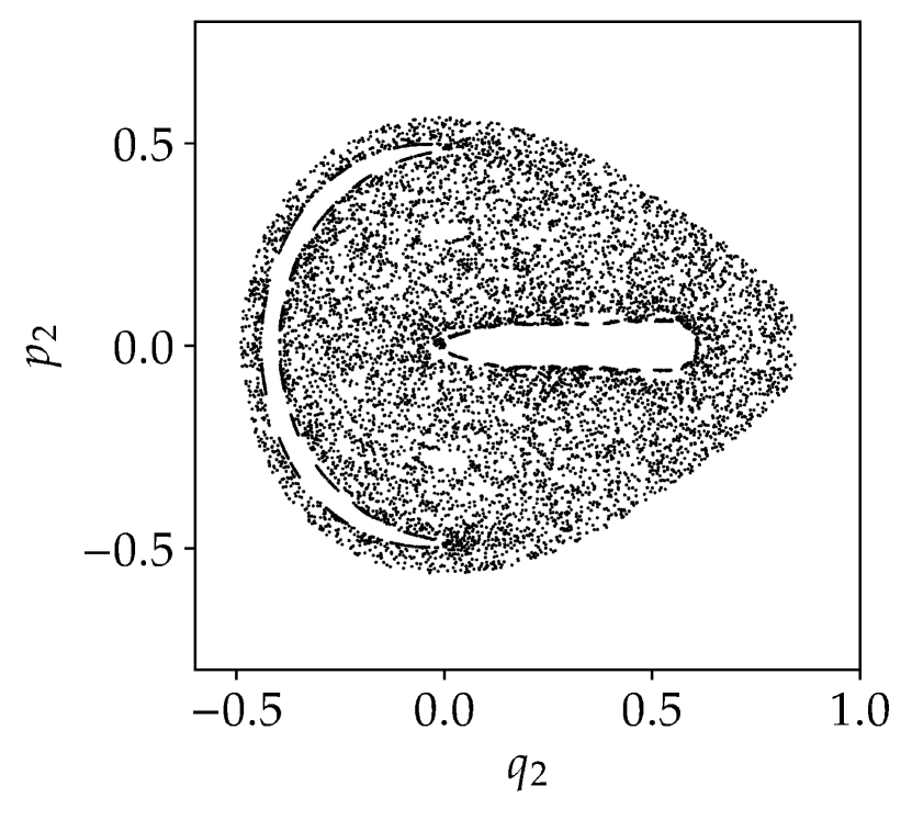
(b) Relaxation scheme.

Figure 3: Poincaré sections of numerical solutions of the Hénon-Heiles system (3.3) with initial condition (3.5) using the third order method SSPRK(3,3) of [43] with and without relaxation and a time step ${\Delta t}=0.1$.

3.3 Duffing Oscillator

The undamped Duffing oscillator

$$\dfrac{\operatorname{d\!}{{}^{2}}}{\operatorname{d\!}{t^{2}}}q(t)=q(t)-q(t)^{3}$$ (3.6)

can be written as a system of first order ODEs using the momentum $p(t)=\dfrac{\operatorname{d\!}{}}{\operatorname{d\!}{t}}q(t)$ and is a Hamiltonian system (1.1) with total energy

$$H(q,p)=\frac{1}{2}p^{2}-\frac{1}{2}q^{2}+\frac{1}{4}q^{4}.$$ (3.7)

The initial condition $(q,p)=(1.4142,0)$ is inside, but very near to, the separatrix (which crosses $(q,p)=(\sqrt{2},0)$) dividing the parts of phase space that give bounded or unbounded solutions [10]. The solution should stay on a closed curve near the separatrix in the half space $q\geq 0$.

Typically, numerical solutions obtained by explicit Runge-Kutta methods i) lose energy and spiral inwards or ii) cross the separatrix and escape to the left half plane, as can be seen in Figure 4. Of course, both behaviors are undesired. The relaxation methods give the correct qualitative behavior.

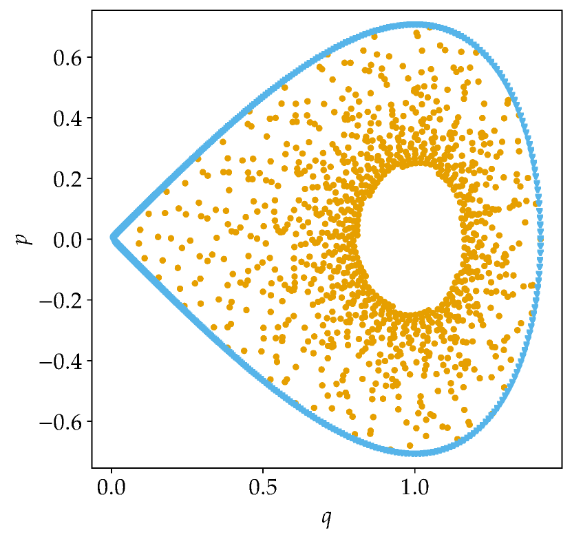
(a) Fourth order method of Kutta [26], with ${\Delta t}=0.5$ and final time $t=500$.

(b) Fifth order method of Bogacki & Shampine [3], with ${\Delta t}=0.25$ and final time $t=5000$.

Figure 4: Simulation of the undamped Duffing oscillator (3.6) using explicit Runge-Kutta methods with and without relaxation to preserve the Hamiltonian.

3.4 Phase Space Volume

Symplectic methods are made to preserve the structure of a Hamiltonian system. While they do not conserve the Hamiltonian exactly in general, a modified Hamiltonian is conserved. Here we investigate whether relaxation Runge-Kutta methods conserving the Hamiltonian show better conservation of phase space volume relative to standard Runge-Kutta methods. While volume preservation is in general not equivalent to symplecticity or approximate energy conservation [20, 18], the change of phase space volume can be measured approximately for some models.

At first, the harmonic oscillator

$$u^{\prime}(t)=Lu(t),\quad u(0)=\begin{pmatrix}1\\ 0\end{pmatrix},\quad L=\begin{pmatrix}0&-1\\ 1&0\\ \end{pmatrix},$$ (3.8)

is considered. To measure the change of phase space volume, $200$ initial conditions are uniformly randomly chosen in a circle of radius $0.001$ around $(1,0)$. These are evolved in time using the symplectic Euler method as well as the unmodified and relaxation version of the classical fourth order Runge-Kutta method with a time step ${\Delta t}=0.25$. The phase space volume occupied by these points is measured by computing the volume of the convex hull of these points using the Qhull library [2] via SciPy [44]. It has been verified by inspection that this approach is reasonable for the test cases under consideration. We choose a symplectic method as reference, since these are constructed to conserve the phase space volume exactly. Additionally, they conserve quadratic Hamiltonians such as the energy of the harmonic oscillator. General Hamiltonians are not conserved exactly by symplectic methods; instead, a modified Hamiltonian is conserved.

The results are shown in Figure 5. Both the symplectic Euler method and the relaxation RK(4,4) method conserve the phase space volume while the baseline RK(4,4) scheme results in a clear loss of phase space volume. A linear fit of the relative change of phase space volume yields the slope $1.15\text{\times}{10}^{-13}$ for the relaxation scheme and $1.07\text{\times}{10}^{-15}$ for the symplectic Euler method.

Additionally, two uncoupled harmonic oscillators are considered as a higher dimensional problem with initial conditions distributed randomly in a cube of side length $0.001$ around $(1,0,0.5,0.5)$. Although both oscillators are uncoupled, total energy conservation via the relaxation approach introduces some coupling. For this case, the slopes of the linear fits of the relative change of phase space volume are $2.13\text{\times}{10}^{-13}$ for the relaxation RK(4,4) method and $-1.72\text{\times}{10}^{-14}$ for the symplectic Euler method.

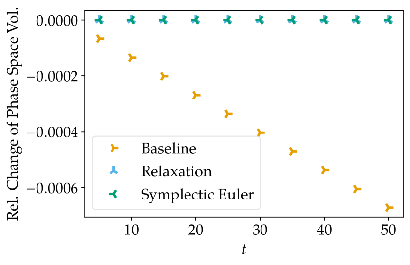
(a) One harmonic oscillator.

(b) Two harmonic oscillators.

Figure 5: Relative change of phase space volume for the harmonic oscillator (3.8) using the symplectic Euler method as well as the classical fourth order Runge-Kutta method RK(4,4) with and without relaxation to preserve the Hamiltonian/energy.

Additionally, the undamped Duffing oscillator (3.6) is considered as a nonlinear example. The $200$ initial conditions are uniformly randomly chosen in a circle of radius $0.001$ around $(1,0)$. The relaxation version of RK(4,4) and SSPRK(3,3) yield visually the same relative change of phas space volume as the symplectic Euler method, while the corresponding baseline schemes result in a clear change of phase space volume, as can be seen in Figure 6. While the appropriateness of the approach to measure the phase space volume has still been verified by inspection, it becomes a bit less exact. In particular, linear fits of the relative change of phase space volume for both relaxation and symplectic methods yield a slope of approximately $1\text{\times}{10}^{-8}$ instead of machine accuracy. For more complicated problems, this approach to measure the phase space volume does not seem to be appropriate.

(a) RK(4,4).

(b) SSPRK(3,3).

Figure 6: Relative change of phase space volume for the Duffing oscillator (3.6) using the symplectic Euler method as well as RK(4,4) and SSPRK(3,3) with and without relaxation to preserve the Hamiltonian.

4 Accuracy

In this section we study the impact of relaxation on accuracy for Hamiltonian problems. It has been observed (and proven in an asymptotic sense) that relaxation does not reduce the order of accuracy of a RK method. Here we show that it can in fact improve the accuracy for Hamiltonian problems. In Section 4.1 we demonstrate that RRK methods reduce the error growth in time for Hamiltonian problems. In Section 4.3 we show that relaxation increases the convergence rate by one for odd order methods applied to a certain class of Hamiltonian problems.

4.1 Error Growth for Oscillatory Problems

Structure preserving methods, especially symplectic or energy conserving ones, result in a good behavior of the numerical error for periodic (Hamiltonian) problems, cf. [8, 29, 9, 7]. For periodic problems where the period is conserved by a relaxation approach, e.g. if the period depends only on the Hamiltonian and the RRK method conserves the Hamiltonian, the asymptotic error growth is linear, even if adaptive time steps are used. This can be proved by applying Theorem 5.1 of [7], noticing that the direction

$$d=\sum_{i=1}^{s}b_{i}f_{i}$$ (4.1)

remains bounded away from zero for ${\Delta t}\to 0$, unless the system is stationary. In contrast, methods that do not preserve some structure of the system (either exactly or to some appropriate order of accuracy) will in general result in an asymptotic error growth that is linear at first and quadratic after some time, usually after the first period, cf. [8, 29, 9, 7].

4.1.1 Nonlinear Oscillator

For the nonlinear oscillator

$$\dfrac{\operatorname{d\!}{}}{\operatorname{d\!}{t}}\begin{pmatrix}u_{1}(t)\\ u_{2}(t)\end{pmatrix}=\mathinner{\!\left\lVert u(t)\right\rVert}^{-2}\begin{pmatrix}-u_{2}(t)\\ u_{1}(t)\end{pmatrix},\quad u^{0}=\begin{pmatrix}1\\ 0\end{pmatrix},$$ (4.2)

of [34, 35], the period is a function of the energy of the solution. Hence, the theory predicts that the error of the baseline Runge-Kutta schemes grows linearly at first and quadratically afterwards while relaxation methods should have a linear error growth in time. The numerical results shown in Figure 7 confirm this theory for the third order method of Heun [23], the fourth order method of Fehlberg [14, Table III], and the fifth order method of Bogacki & Shampine [3].

(a) Third order method of Heun [23], ${\Delta t}=0.025$.

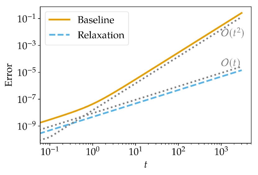
(b) Fourth order method of Fehlberg [14, Table III], ${\Delta t}=0.1$.

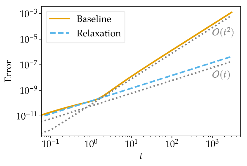
(c) Fifth order method of Bogacki & Shampine [3], ${\Delta t}=0.1$.

Figure 7: Error growth in time for the nonlinear oscillator (4.2) using different baseline and relaxation Runge-Kutta methods.

4.1.2 Kepler Problem

The Kepler problem

$$\begin{gathered}\dfrac{\operatorname{d\!}{}}{\operatorname{d\!}{t}}q(t)=\dfrac{\operatorname{d\!}{}}{\operatorname{d\!}{t}}\begin{pmatrix}q_{1}(t)\\ q_{2}(t)\end{pmatrix}=p(t),\quad\dfrac{\operatorname{d\!}{}}{\operatorname{d\!}{t}}p_{i}(t)=-\frac{q_{i}(t)}{\mathinner{\!\left\lvert q(t)\right\rvert}^{3}},\\ q(0)=\begin{pmatrix}1-e\\ 0\end{pmatrix},\quad p(0)=\begin{pmatrix}0\\ \sqrt{(1-e)/(1+e)}\end{pmatrix},\end{gathered}$$ (4.3)

with eccentricity $e=0.5$ is a Hamiltonian system (1.1) with Hamiltonian

$$H(q,p)=\frac{1}{2}\mathinner{\!\left\lvert p\right\rvert}^{2}-\frac{1}{\mathinner{\!\left\lvert q\right\rvert}},$$ (4.4)

where the angular momentum

$$L(q,p)=q_{1}p_{2}-q_{2}p_{1}$$ (4.5)

is an additional conserved quantity, cf. [41, 8, Section 1.2.4]. The period depends only on the Hamiltonian, which can be conserved by relaxation Runge-Kutta methods. Another possibility is to employ the relaxation approach to conserve the angular momentum.

Results of baseline schemes, RRK methods conserving the Hamiltonian, and RRK methods conserving the angular momentum are shown in Figure 8. As expected, the asymptotic error growth is quadratic whenever the Hamiltonian is not conserved while the energy conserving RRK methods result in a linear error growth in time, similarly to symplectic schemes.

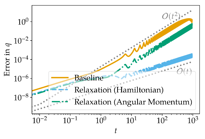
(a) Third order method of Shu & Osher [43], ${\Delta t}=0.001$.

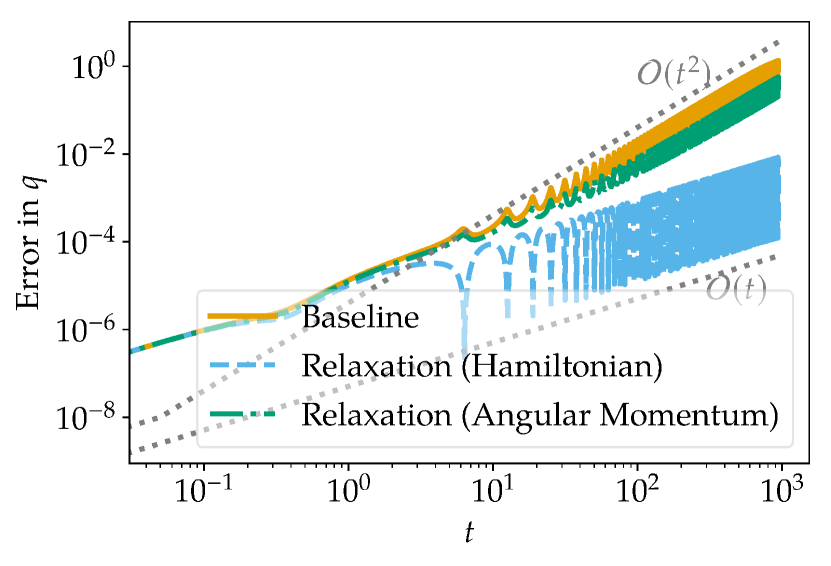
(b) Fourth order method of Kutta [26], ${\Delta t}=0.05$.

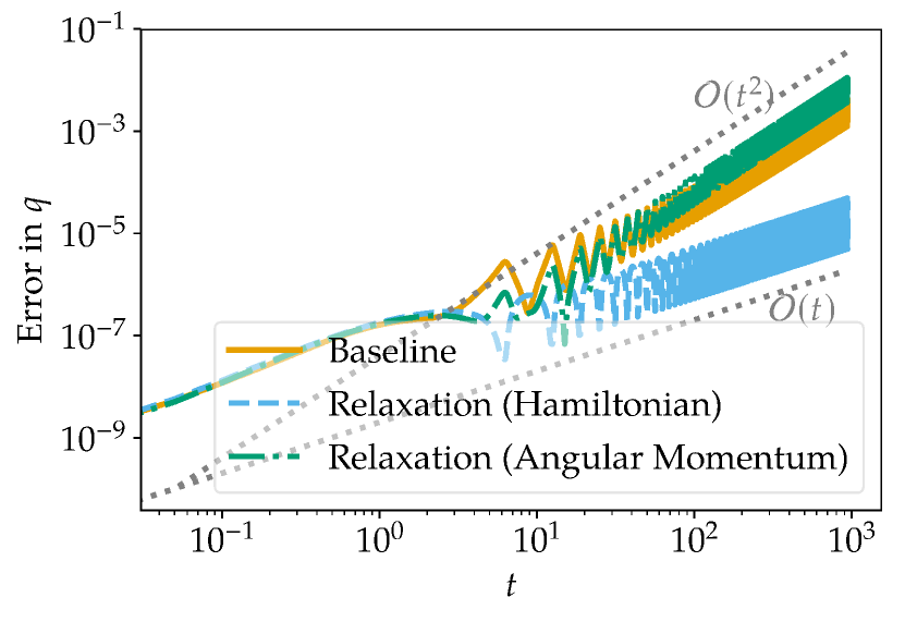
(c) Fifth order method of Prince & Dormand [30], ${\Delta t}=0.05$.

Figure 8: Error growth in time for the Kepler problem (4.3) using different baseline and relaxation Runge-Kutta methods.

4.1.3 Korteweg-de Vries Equation

The Korteweg-de Vries (KdV) equation

$$\partial_{t}u+\partial_{x}\frac{u^{2}}{2}+\partial_{x}^{3}u=0$$ (4.6)

is well-known in the literature as a nonlinear PDE which admits soliton solutions of the form

$$u(t,x)=A\cosh\bigl{(}\sqrt{3A}(x-ct-\mu)/6\bigr{)}^{-2},\quad c=\nicefrac{{A}}{{3}},$$ (4.7)

where $A$ is the amplitude, $c$ the wave speed, and $\mu$ an arbitrary constant. The KdV equation possesses an infinite hierarchy of conserved quantities, including the mass $\int u$ and the energy $\frac{1}{2}\mathinner{\!\left\lVert u\right\rVert}^{2}=\frac{1}{2}\int u^{2}$.

Using periodic boundary conditions, mass- and energy-conservative semidiscretizations using central finite difference or Fourier collocation schemes can be constructed using a split form as

$$\partial_{t}u+\frac{1}{3}\bigl{(}D_{1}(u\cdot u)+u\cdot(D_{1}u)\bigr{)}+D_{3}u=0,$$ (4.8)

where $D_{k}$ is the discrete derivative operator approximating the $k$th derivative, i.e. $D_{k}u\approx\partial_{x}^{k}u$. Here $u$ is the vector of solution values at the spatial grid points, and $\cdot$ denotes elementwise multiplication. The semidiscretization (4.8) is obtained by averaging the conservative form $\partial_{x}\nicefrac{{u^{2}}}{{2}}$ of the nonlinear term and the equivalent form $u\partial_{x}u$. Such split forms are often necessary to obtain conservative or dissipative semidiscretizations of nonlinear PDEs since the product and chain rules do not hold discretely [33]. Although the idea to use split forms is not new [39, eq. (6.40)], it is still state of the art [15, 32].

In the context of structure preserving schemes, especially energy conservative schemes, the KdV equation has been studied in [40, 42, 12]. In particular, the error growth in time for soliton solutions has been studied in [12], where it is proved that mass- and energy-conservative discretizations result in an asymptotically linear error growth while other discretizations yield a quadratically growing error in time.

To study the behavior of relaxation Runge-Kutta methods for the KdV equation, the domain $[-20,60]$ is discretized using a pseudospectral Fourier collocation method (4.8) with $N=256$ nodes. With this semi-discretization, it is expected that the temporal error will be dominant unless very small time steps are used. Since the third derivative in space results in a stiff semi-discrete problem, implicit Runge-Kutta methods are advantageous. Here, the two stage, third order SDIRK method of Nørsett [28] given in [21, Table II.7.2] is used with a time step ${\Delta t}=0.5$ to advance till the final time $t=600$. The stage equations are solved using fsolve from SciPy [44]. This SDIRK method has also been used as an example in [12] (without relaxation or orthogonal projection). The initial condition is given as the projection of the soliton with amplitude $A=2$ and offset $\mu=40$. We also test the behavior of this discretization when orthogonal projection is applied (instead of relaxation) in order to preserve energy.

As can be seen in Figure 9, the relaxation and projection methods conserve the total energy up to small errors (due to roundoff and errors in the solution of the projection equation) while the baseline SDIRK method results in a decaying energy. The relaxation method, due to its linear covariance, also preserves the mass, while the projection method does not (indeed, over the course of the simulation the projection method leads to a mass increase of almost $10\text{\,}\mathrm{\char 37\relax}$). In accordance with the theory of [12], the error of the baseline scheme grows quadratically in time until it saturates at $100\text{\,}\mathrm{\char 37\relax}$ error. In contrast, the energy conservative RRK method yields a linearly growing error in time. This results in a much smaller error at the final time, yielding a numerical solution that is visually indistinguishable from the analytical one, as shown in Figure 10(a). The projection method also exhibits linear growth for some time, but at very long times shows quadratic growth due to a noticeable phase error in Figure 10(a). This is again in accordance with the theory of [12], since the total mass is not conserved. Similar results have been obtained for the fourth order SDIRK methods SDIRK(3,4) of [22, Table IV.6.5] and SDIRK(5,4) of [22, eq. (6.18)].

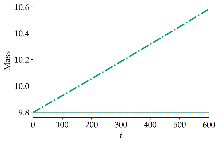
(a) Mass of numerical solutions.

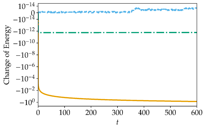
(b) Energy of numerical solutions.

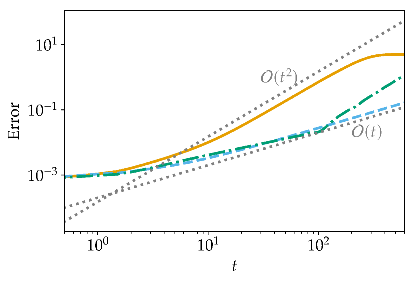
(c) Error of numerical solutions.

Figure 9: Total masses & energies and errors of numerical solutions with and without relaxation to preserve the energy for the KdV equation (4.8).

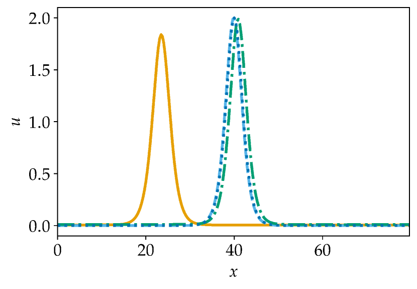
(a) Analytical and numerical solutions at the final time with and without relaxation.

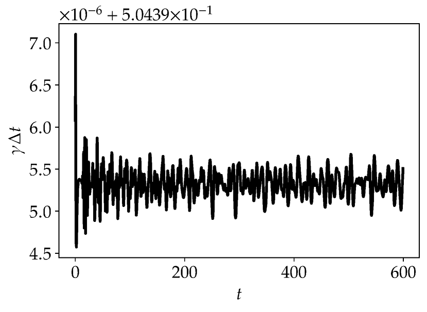
(b) Scaled time step $\gamma{\Delta t}$ used by the relaxation method.

Figure 10: Results of numerical experiments with final time $t=600$ for the KdV equation (4.8).

Based on observations for this problem, relaxation methods are particularly interesting for implicit Runge-Kutta schemes. Firstly, the cost of solving the scalar equation for the relaxation parameter $\gamma$ is negligible compared to the cost of solving the stage equations. Secondly, the relaxation approach can result in larger scaled time steps $\gamma{\Delta t}>{\Delta t}$. For the scheme considered in this example, the baseline method uses time steps ${\Delta t}=0.5$ while the scaled timesteps $\gamma{\Delta t}$ of the relaxation method were slightly larger with a median $\approx 0.504$, resulting in fewer time steps needed to reach the final time, cf. Figure 10(b).

4.2 Some Remarks on the Costs of Relaxation

We have used SciPy [44] to solve the scalar equations for the relaxation parameter $\gamma$. The implementations make use of functions written in pure Python and are not adapted to the specific problems. A detailed assessment of the computational cost of solving for $\gamma$ would require a more refined implementation and is beyond the scope of this work. Nevertheless, we give some preliminary discussion of the costs here, emphasizing that these numbers should be viewed as very loose upper bounds on the cost of relaxation.

If an explicit time-stepping method is used and the evaluation of the right-hand side is inexpensive, the costs of naive implementations of the relaxation approach are significant. For example, solving the Lotka-Volterra system with RK4 as discussed in Section 3.1 takes $5.14\text{\times}{10}^{-02}\text{\,}\mathrm{s}$ without relaxation and $1.18\text{\times}{10}^{-01}\text{\,}\mathrm{s}$ with relaxation. The phase space plot of the baseline scheme can be made to be visually indistinguishable from the one of the relaxation method by reducing the time step by a factor of four, resulting in a CPU time of $1.97\text{\times}{10}^{-01}\text{\,}\mathrm{s}$. Although the relaxation technique increases the runtime significantly in this naive implemetation, it is still cheaper than decreasing the time step to get basically the same results.

When implicit time-stepping is used, the cost of relaxation is less significant. For the KdV equation discussed in Section 4.1.3, the baseline method needs $6.36\text{\times}{10}^{01}\text{\,}\mathrm{s}$, the relaxation method needs $6.26\text{\times}{10}^{01}\text{\,}\mathrm{s}$, and the projection method needs $6.30\text{\times}{10}^{01}\text{\,}\mathrm{s}$. We see that the energy-conserving methods decrease the runtime despite the added overhead of computing the relaxation or projection step. This can be explained by noting that these methods yield improved accuracy and hence decreased costs to solve the nonlinear stage equations. The relaxation method benefits additionally from taking larger effective time steps since the relaxation parameter $\gamma>1$.

4.3 Superconvergence for Euclidean Hamiltonian Problems

The simplest Hamiltonian system is the harmonic oscillator (3.8). In Figure 11 we present convergence results for this problem, integrated to final time $10$ and using four RK methods of orders two to five. In the absence of relaxation, each scheme exhibits the expected order of convergence. When relaxation is applied, the odd-order schemes converge with a rate one order faster than their formal order.

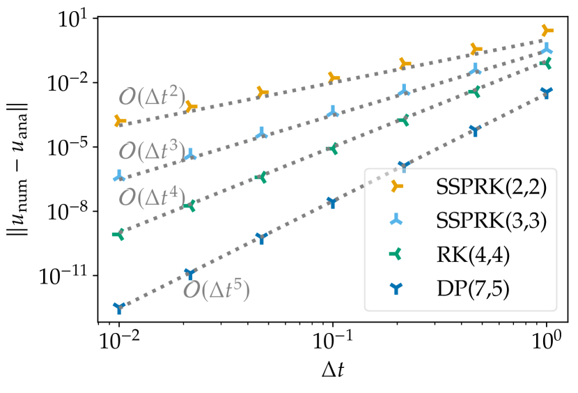
(a) Baseline schemes.

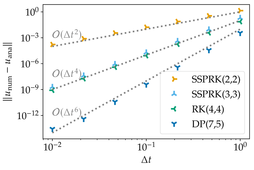
(b) Relaxation schemes.

Figure 11: Convergence study using baseline Runge-Kutta and relaxation schemes for the harmonic oscillator (3.8). DP(7,5) is the fifth order method of Prince & Dormand [30].

Next, consider the nonlinear oscillator (4.2). In Figure 12 we present convergence results for this problem, integrated to final time $10$, again using RK methods of orders two to five (but with different 3rd- and 5th-order methods than in the previous example). Again, the methods converge at the expected rate without relaxation, but the odd-order methods show an increased rate of convergence when relaxation is applied. Interestingly, the relaxation version of Heun’s method has a significantly smaller error than the classical RK(4,4) scheme, both with and without relaxation.

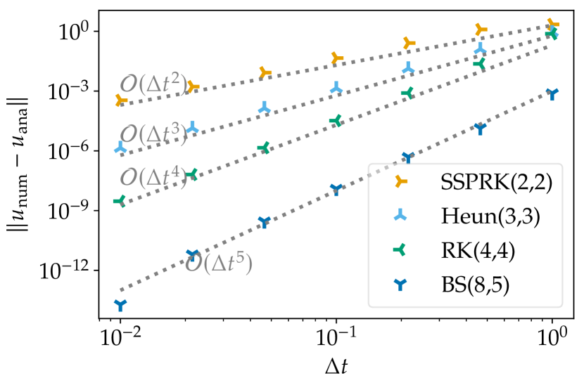
(a) Baseline schemes.

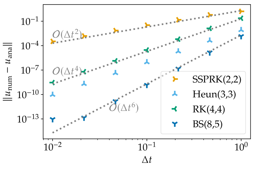
(b) Relaxation schemes.

Figure 12: Convergence study using baseline Runge-Kutta and relaxation schemes for the nonlinear oscillator (4.2). BS(8,5) is the fifth order method of Bogacki & Shampine [3].

These two examples suggest a general result that we will state next. Consider a Hamiltonian $H$ that is a smooth function of the squared Euclidean norm, i.e.

$$H(q,p)=G\bigl{(}(|q|^{2}+|p|^{2})/2\bigr{)},$$ (4.9)

where $G$ is a smooth function. The corresponding Hamiltonian system is

$$\begin{cases}u^{\prime}(t)=f(u(t)),\\ u(0)=u_{0},\end{cases}\quad u(t)=\begin{pmatrix}q(t)\\ p(t)\end{pmatrix},\quad f(q,p)=g\bigl{(}(|q|^{2}+|p|^{2})/2\bigr{)}\begin{pmatrix}p\\ -q\end{pmatrix},$$ (4.10)

where $g=G^{\prime}$. We refer to (4.10) as a Euclidean Hamiltonian problem. For this class of problems, nominally odd order relaxation Runge-Kutta methods are superconvergent.

Theorem 4.1.

Consider the general nonlinear Euclidean Hamiltonian system (4.10) and a Runge-Kutta method of order $p$ with $s$ stages. The corresponding RRK scheme conserving the Hamiltonian has an order of accuracy $p+1$ if $p$ is odd.

Remark 4.2.

Every skew-symmetric linear system in two space dimensions satisfies the Euclidean Hamiltonian structure above. Linear skew-symmetric systems in three space dimensions must have a zero eigenvalue and can consequently be reduced to a skew-symmetric system in two space dimensions.

Remark 4.3.

Since $H$ is conserved, the analytical solution of any Euclidean Hamiltonian problem evolves identically to that of the corresponding linear system (with fixed value of $g(u)=g(u_{0})$)

$$\begin{cases}u^{\prime}(t)=f(u(t)),\\ u(0)=u_{0},\end{cases}\quad u(t)=\begin{pmatrix}q(t)\\ p(t)\end{pmatrix},\quad f(q,p)=g\bigl{(}(|q_{0}|^{2}+|p_{0}|^{2})/2\bigr{)}\begin{pmatrix}p\\ -q\end{pmatrix}.$$ (4.11)

The proof of Theorem 4.1 is presented in Appendix A. As can be seen there, the Euclidean Hamiltonian structure is crucial. In particular, the result does not hold for general skew-symmetric linear systems conserving the Euclidean norm, e.g.

$$u^{\prime}(t)=Lu(t),\quad u(0)=\begin{pmatrix}1\\ 0\\ 0\\ 0\end{pmatrix},\quad L=\begin{pmatrix}0&0&-1&-1\\ 0&0&0&-1\\ 1&0&0&-1\\ 1&1&1&0\end{pmatrix}.$$ (4.12)

Furthermore, the superconvergence result does not hold for general linear Hamiltonian systems where the Hamiltonian is not an affine function of the squared Euclidean norm, e.g.

$$\begin{gathered}\dfrac{\operatorname{d\!}{}}{\operatorname{d\!}{t}}\begin{pmatrix}q(t)\\ p(t)\end{pmatrix}=\begin{pmatrix}0&\operatorname{I}\\ -\operatorname{I}&0\end{pmatrix}\nabla_{(q,p)}H(q,p),\quad H(q,p)=\frac{1}{2}q^{T}Qq+\frac{1}{2}p^{T}Pp,\\ Q=\begin{pmatrix}1&1\\ 1&2\end{pmatrix},\quad P=\begin{pmatrix}3&2\\ 2&4\end{pmatrix},\quad q(0)=\begin{pmatrix}1\\ 0\end{pmatrix},\quad p(0)=\begin{pmatrix}0\\ 0\end{pmatrix}.\end{gathered}$$ (4.13)

We have conducted further numerical experiments, supporting the hypothesis that the superconvergence property of RRK schemes is restricted to Euclidean Hamiltonian ones.

5 $N$-Body Applications

Energy preservation is particularly important in the solution of $N$-body problem arising in astrophysics and molecular dynamics. In this section we investigate the behavior of RRK methods on problems from these two areas.

5.1 Outer Solar System

Consider the outer solar system consisting of the sun (including the mass of the inner planets), Jupiter, Saturn, Uranus, Neptune, and Pluto This can be described by a Hamiltonian system with

$$H(p,q)=\frac{1}{2}\sum_{i=0}^{5}\frac{1}{m_{i}}p_{i}^{T}p_{i}-G\sum_{i=1}^{5}\sum_{j=0}^{i-1}\frac{m_{i}m_{j}}{\|q_{i}-q_{j}\|}.$$

We take the masses and initial data exactly as given in [19, Section I.2.3]. Applying the second order accurate method SSPRK(2,2) with a (rather large) time step size of ${\Delta t}=200$ (days) for a total time of $200\,000$ (days) yields the results shown in Figure 13. While the orbits should be essentially stationary on this time scale, the numerical approximation yields perturbed orbits with a drift of the radius, which is most pronounced for the planets with the shortest orbits. Additionally, the Hamiltonian (energy) grows considerably over time.

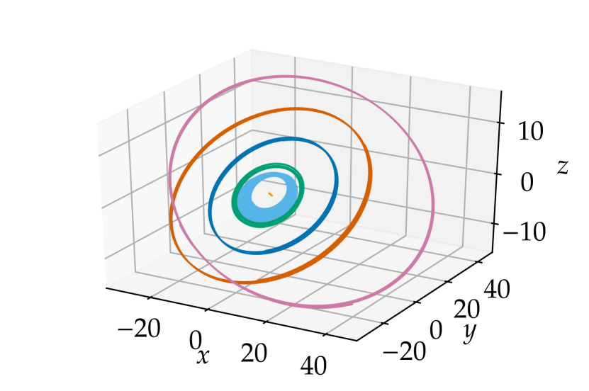
(a) Orbits of the planets and the sun.

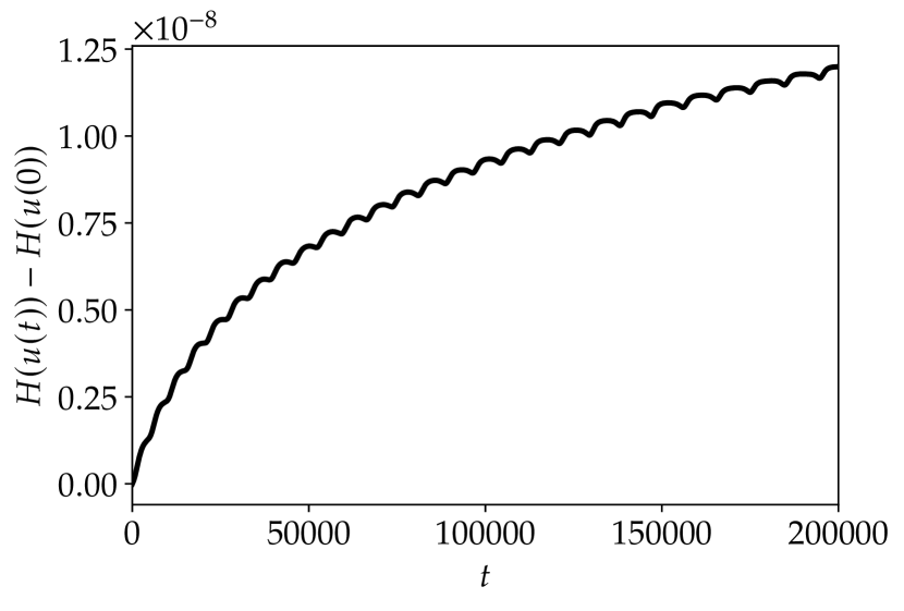
(b) Change of the Hamiltonian over time.

Figure 13: Simulation of the outer solar system using the baseline SSPRK(2,2) method.

Applying the relaxation approach to preserve the Hamiltonian during the simulation does not necessarily increase the quality of the numerical approximation in this case, as can be seen in Figure 14. While the relaxation approach yields a constant (to machine accuracy) Hamiltonian, the deviation in the orbits is similar or even worse. This is in general agreement with the observations of [19, Example IV.4.4], where projection methods conserving the Hamiltonian or even the Hamiltonian and the angular momentum do not necessarily improve the quality of the numerical solution. On the contrary, some orbits become even worse when applying the projection methods used there. As stated in [19, Example IV.4.4]: “There is no doubt that this problem contains a structure which cannot be correctly simulated by methods that only preserve the total energy $H$ and the angular momentum $L$”.

(a) Orbits of the planets and the sun.

(b) Change of the Hamiltonian over time.

Figure 14: Simulation of the outer solar system using SSPRK(2,2) with relaxation to preserve the Hamiltonian (energy).

5.2 Molecular Dynamics

For the outer solar system discussed in the previous section, the orbit of each body is important and has to be preserved as much as possible. In contrast, in molecular dynamics simulations “we do not need exact classical trajectories… but must lay great emphasis on energy conservation as being of primary importance.” [1, p. 99] Thus it is reasonable to expect that energy conserving relaxation Runge-Kutta methods can be applied advantageously to molecular dynamics simulations.

Consider the example of a frozen argon crystal described by Hairer, Lubich, and Wanner [19, Section I.3.2], consisting of argon atoms interacting via the classical Lennard-Jones potential with an initial condition close to the minimum energy state. As mentioned above, our interest here is in statistical quantities such as the total energy (Hamiltonian) and the temperature. While the Hamiltonian is conserved, the temperature is expected to fluctuate around a certain mean value. These properties are not preserved in general by numerical discretizations.

Results of simulations of this system using the classical fourth order Runge-Kutta method RK(4,4) with and without relaxation to preserve the total energy are shown in Figure 15. As can be seen, the baseline scheme yields significant drift in the energy and temperature. Using instead the relaxation approach, the Hamiltonian is conserved and the temperature fluctuates around a mean value without significant drift.

To be competitive for molecular dynamics simulations, the cost of the relaxation approach also has to be considered. While only a scalar equation has to be solved per time step, it involves a computation of the energy which is similarly expensive as computing the forces. Hence, specialised implementations and considerations of using adapted or inexact solutions for the relaxation parameter $\gamma$ should be investigated, which is out of the scope of this article.

(a) Baseline RK(4,4).

(b) RK(4,4) with relaxation.

Figure 15: Simulation of the frozen argon crystal with and without relaxation to preserve the Hamiltonian.

6 Conclusions

We have studied relaxation Runge-Kutta (RRK) methods in the context of differential equations with nonlinear invariants, especially Hamiltonian systems. Similar to other structure preserving numerical schemes, RRK methods result in an improved qualitative behavior of numerical solutions, concerning e.g. the preservation of orbits or Poincaré sections (Section 3). Additionally, they share advantageous quantitative properties with symplectic methods such as a linear error growth for certain classes of Hamiltonian problems (Section 4.1). Furthermore, RRK methods show a superconvergence property for Euclidean Hamiltonian systems (Section 4.3). Finally, our limited results suggest that RRK methods may be useful for Hamiltonian problems, such as those in molecular dynamics, where statistical averages are of interest (Section 5).

For some classes of Hamiltonian problems, explicit symplectic methods such as the Störmer Verlet scheme are available. Compared to these methods, RRK methods have to solve a single scalar equation per time step which can be a certain bottleneck. To be fully competetive, specialised implementations will studied in a future work. On the other hand, RRK methods can be of arbitrary order and allow more freedom in their design.

Whenever implicit schemes are advantageous, e.g. because of stiffness restrictions, the relaxation approach provides an inexpensive means to conserve important nonlinear quantities, which is usually only possible for fully implicit methods. Hence, diagonally implicit RRK methods seem very competitive for such problems. In future work, we plan to deepen the investigation of RRK methods in this context and study the combination of the relaxation approach with several classes of schemes such as implicit-explicit (IMEX) methods and splitting algorithms.

Another direction of future research is the application of relaxation to enforce conservation with a Hamiltonian PDE semi-discretization that is not conservative. In this context the relaxation process would be used to remove the conservation error created by the spatial discretization. Some numerical experiments (not included here) suggest that the relaxation approach can be applied successfully in this context as long as the discretization errors in space and time are of a similar order of magnitude. Nevertheless, deeper theoretical and empirical studies are necessary.

Appendix A Superconvergence Theorem Proofs

To facilitate the proof of the general result 4.1, we first present and prove a version restricted to linear problems.

Theorem A.1.

Consider the linear Euclidean Hamiltonian system

$$\begin{cases}u^{\prime}(t)=Lu(t),\\ u(0)=u_{0},\end{cases}\quad u(t)=\begin{pmatrix}q(t)\\ p(t)\end{pmatrix},\quad L=\alpha\begin{pmatrix}0&\operatorname{I}\\ -\operatorname{I}&0\end{pmatrix}.$$ (A.1)

and an explicit Runge-Kutta method of order $p\in\mathbb{N}$ with $s\geq p$ stages. The corresponding RRK scheme conserving the Hamiltonian has an order of accuracy $p+1$ if $p$ is odd.

In the proof of Theorem A.1, the following lemma will be used.

Lemma A.2.

For $s,m\in\mathbb{N}$, $2m\leq s+1$,

$$\sum_{n=\max\mathinner{\left\{1-m,m-s\right\}}}^{\min\mathinner{\left\{m-1,s-m\right\}}}(-1)^{n}\frac{1}{(m-n)!(m+n)!}=-2(-1)^{m}\frac{1}{(2m)!}.$$ (A.2)

Proof.

Use some explicit calculations or the Mathematica [45] notebook Combinatorial_Lemma.nb in the repository [36]. ∎

Proof of Theorem A.1.

It suffices to consider the first step. The baseline RK method starting from $u_{0}$ yields

$$u_{+}=u_{0}+\sum_{k=1}^{s}\alpha_{k}{\Delta t}^{k}L^{k}u_{0},$$ (A.3)

where $\alpha_{k}$ are the monomial coefficients of the corresponding stability polynomial. The relaxation method results in the new value

$$u_{+}^{\gamma}=u_{0}+\gamma\sum_{k=1}^{s}\alpha_{k}{\Delta t}^{k}L^{k}u_{0}$$ (A.4)

with squared Euclidean norm

$$\mathinner{\!\left\lVert u_{+}^{\gamma}\right\rVert}^{2}=\left(2\gamma\sum_{l=1}^{\lfloor s/2\rfloor}(-1)^{l}\alpha_{2l}{\Delta t}^{2l}\mathinner{\!\left\lVert L^{l}u_{0}\right\rVert}^{2}+\gamma^{2}\sum_{\mathclap{\begin{subarray}{c}j,k=1\\ j+k\text{ even}\end{subarray}}}^{s}(-1)^{(j-k)/2}\alpha_{j}\alpha_{k}h^{j+k}\mathinner{\!\left\lVert L^{(j+k)/2}u_{0}\right\rVert}^{2}\right)\mathinner{\!\left\lVert u_{0}\right\rVert}^{2}.$$ (A.5)

The second sum can also be written as

$$\sum_{\mathclap{\begin{subarray}{c}j,k=1\\ j+k\text{ even}\end{subarray}}}^{s}\alpha_{j}\alpha_{k}(-1)^{(j-k)/2}h^{j+k}\mathinner{\!\left\lVert L^{(j+k)/2}u_{0}\right\rVert}^{2}=\sum_{m=1}^{s}\sum_{n=\max\mathinner{\left\{1-m,m-s\right\}}}^{\min\mathinner{\left\{m-1,s-m\right\}}}(-1)^{n}\alpha_{m-n}\alpha_{m+n}\mathinner{\!\left\lVert L^{m}u_{0}\right\rVert}^{2}.$$ (A.6)

The non-zero value of the relaxation parameter conserving the Euclidean norm is

$$\gamma=\frac{-2\sum_{l=1}^{\lfloor s/2\rfloor}(-1)^{l}\alpha_{2l}{\Delta t}^{2l}\mathinner{\!\left\lVert L^{l}u_{0}\right\rVert}^{2}}{\sum_{m=1}^{s}\sum_{n=\max\mathinner{\left\{1-m,m-s\right\}}}^{\min\mathinner{\left\{m-1,s-m\right\}}}(-1)^{n}\alpha_{m-n}\alpha_{m+n}\mathinner{\!\left\lVert L^{m}u_{0}\right\rVert}^{2}}.$$ (A.7)

For a $p$-th order baseline scheme,

$$\alpha_{k}=\frac{1}{k!},\qquad k\in\mathinner{\left\{1,\dots,p\right\}}.$$ (A.8)

Hence, for odd $p$, the numerator of $\gamma$ (A.7) is

$$-2\sum_{l=1}^{\lfloor s/2\rfloor}(-1)^{l}\alpha_{2l}{\Delta t}^{2l}\mathinner{\!\left\lVert L^{l}u_{0}\right\rVert}^{2}\\ =-2\sum_{l=1}^{\lfloor p/2\rfloor}(-1)^{l}\frac{1}{(2l)!}{\Delta t}^{2l}\mathinner{\!\left\lVert L^{l}u_{0}\right\rVert}^{2}-2(-1)^{(p+1)/2}\alpha_{p+1}{\Delta t}^{p+1}\mathinner{\!\left\lVert L^{(p+1)/2}u_{0}\right\rVert}^{2}+\mathcal{O}({\Delta t}^{p+3}).$$ (A.9)

Because of Lemma A.2, the denominator of $\gamma$ (A.7) for odd $p$ is

$$\sum_{m=1}^{s}\sum_{n=\max\mathinner{\left\{1-m,m-s\right\}}}^{\min\mathinner{\left\{m-1,s-m\right\}}}(-1)^{n}\alpha_{m-n}\alpha_{m+n}\mathinner{\!\left\lVert L^{m}u_{0}\right\rVert}^{2}\\ =-2\sum_{m=1}^{\lfloor p/2\rfloor}(-1)^{m}\frac{1}{(2m)!}\mathinner{\!\left\lVert L^{m}u_{0}\right\rVert}^{2}-2(-1)^{(p+1)/2}\frac{1}{(p+1)!}{\Delta t}^{p+1}\mathinner{\!\left\lVert L^{(p+1)/2}u_{0}\right\rVert}^{2}+\mathcal{O}({\Delta t}^{p+3}).$$ (A.10)

Thus,

$$\gamma=1-2(-1)^{(p+1)/2}\left(\alpha_{p+1}-\frac{1}{(p+1)!}\right){\Delta t}^{p-1}\frac{\mathinner{\!\left\lVert L^{(p+1)/2}u_{0}\right\rVert}^{2}}{\mathinner{\!\left\lVert Lu_{0}\right\rVert}^{2}}+\mathcal{O}({\Delta t}^{p+1}).$$ (A.11)

Comparing the analytical solution

$$u(\gamma{\Delta t})=\left(\sum_{k=0}^{\infty}\frac{\gamma^{k}{\Delta t}^{k}}{k!}L^{k}\right)u_{0}$$ (A.12)

with the RRK solution,

$$u_{+}^{\gamma}-u(\gamma{\Delta t})=\left(\sum_{k=1}^{p}\frac{1}{k!}(\gamma-\gamma^{k}){\Delta t}^{k}L^{k}\right)u_{0}+\left(\alpha_{p+1}\gamma-\frac{\gamma^{p+1}}{(p+1)!}\right){\Delta t}^{p+1}L^{p+1}u_{0}+\mathcal{O}({\Delta t}^{p+2}).$$ (A.13)

Inserting $\gamma$ (A.11) and expanding the term $(\gamma-\gamma^{2}){\Delta t}^{2}L^{2}u_{0}$ results in

$$u_{+}^{\gamma}-u(\gamma{\Delta t})=\left(\alpha_{p+1}-\frac{1}{(p+1)!}\right)\left((-1)^{(p+1)/2}\frac{\mathinner{\!\left\lVert L^{(p+1)/2}u_{0}\right\rVert}^{2}}{\mathinner{\!\left\lVert Lu_{0}\right\rVert}^{2}}L^{2}u_{0}+L^{p+1}u_{0}\right){\Delta t}^{p+1}+\mathcal{O}({\Delta t}^{p+2}).$$ (A.14)

Finally, the second term in brackets vanishes because of the special structure of $L$ (A.1). ∎

To prove Theorem 4.1, expansions using rooted trees will be applied, cf. [4, Chapter 3]. The following structural results will be used.

Lemma A.3.

For the Euclidean Hamiltonian system (4.10), $m\in\mathbb{N}$, and $n\in\mathinner{\left\{0,\dots,m\right\}}$, there exists a smooth function $h_{m,n}$ such that

$$f^{(m)}(\underbrace{f,\dots,f}_{n\text{ terms}},\underbrace{u,\dots,u}_{m-n\text{ terms}})=\begin{cases}h_{m,n}(\mathinner{\!\left\lVert u\right\rVert}^{2}/2)f(u),&\text{if }n\text{ is even},\\ h_{m,n}(\mathinner{\!\left\lVert u\right\rVert}^{2}/2)u,&\text{if }n\text{ is odd}.\end{cases}$$ (A.15)

Proof by induction.

The induction hypothesis is fulfilled for the basic cases $m=1$ & $n\in\mathinner{\left\{0,1\right\}}$, since

$$\begin{gathered}f^{\prime}(q,p)=\begin{pmatrix}g^{\prime}pq^{T}&g^{\prime}pp^{T}+g\operatorname{I}\\ -g^{\prime}qq^{T}-g\operatorname{I}&-g^{\prime}qp^{T}\end{pmatrix},\\ f^{\prime}f=-g^{2}\begin{pmatrix}q\\ p\end{pmatrix}\propto u,\quad f^{\prime}u=\bigl{(}g^{\prime}(|q|^{2}+|p|^{2})+g\bigr{)}\begin{pmatrix}p\\ -q\end{pmatrix}\propto f,\end{gathered}$$ (A.16)

and $g,g^{\prime}$ depend on $\mathinner{\!\left\lVert u\right\rVert}^{2}$.

The induction step from $m$ to $m+1$ can be carried out by differentiating the identity (A.15). For even $n$, the derivative with respect to $u^{j}$ of the right hand side is

$$\partial_{j}h_{m,n}f^{i}=h_{m,n}^{\prime}u^{j}f^{i}+h_{m,n}f^{i}_{j}.$$ (A.17)

Multiplication by $u^{j}$ and $f^{j}$, respectively, yield

$$(\partial_{j}h_{m,n}f^{i})u^{j} =(h_{m,n}^{\prime}\mathinner{\!\left\lVert u\right\rVert}^{2}+g^{\prime}\mathinner{\!\left\lVert u\right\rVert}^{2}+g)f^{i},$$ (A.18)

$$(\partial_{j}h_{m,n}f^{i})f^{j} =-g^{2}h_{m,n}u^{i}.$$

Similarly, for odd $n$, the derivative of the right hand side is

$$\partial_{j}h_{m,n}u^{i}=h_{m,n}^{\prime}u^{j}u^{i}+h_{m,n}\delta^{i}_{j}$$ (A.19)

and multiplication by $u^{j}$ and $f^{j}$, respectively, result in

$$(\partial_{j}h_{m,n}u^{i})u^{j} =(h_{m,n}^{\prime}\mathinner{\!\left\lVert u\right\rVert}^{2}+h_{m,n})u^{i},$$ (A.20)

$$(\partial_{j}h_{m,n}u^{i})f^{j} =h_{m,n}f^{i}.$$

For all $n$, multiplication of the derivative of the right hand side by $u^{j}$ doesn’t change the direction while multiplication by $f^{j}$ flips the direction from $u$ to $f$ and vice versa.

The derivative with respect to $u^{j}$ of the left hand side of (A.15) is

$$\quad\partial_{j}f^{i}_{j_{1}\dots j_{m}}f^{j_{1}}\dots f^{j_{n}}u^{j_{n+1}}\dots u^{j_{m}}$$ (A.21)

$$=f^{i}_{j_{1}\dots j_{m}j}f^{j_{1}}\dots f^{j_{n}}u^{j_{n+1}}\dots u^{j_{m}}$$

$$\quad+f^{i}_{j_{1}\dots j_{m}}f^{j_{1}}_{j}f^{j_{2}}\dots f^{j_{n}}u^{j_{n+1}}\dots u^{j_{m}}+\dots+f^{i}_{j_{1}\dots j_{m}}f^{j_{1}}\dots f^{j_{n-1}}f^{j_{n}}_{j}u^{j_{n+1}}\dots u^{j_{m}}$$

$$\quad+f^{i}_{j_{1}\dots j_{m}}f^{j_{1}}\dots f^{j_{n}}\delta^{j_{n+1}}_{j}u^{j_{n+2}}\dots u^{j_{m}}+\dots+f^{i}_{j_{1}\dots j_{m}}f^{j_{1}}\dots f^{j_{n}}u^{j_{n+1}}\dots u^{j_{m-1}}\delta^{j_{m}}_{j}.$$

Multiplication of all but the first term on the right hand side by $u^{j}$ doesn’t change the direction while multiplication by $f^{j}$ flips the direction from $u$ to $f$ and vice versa, exactly as for the derivative of the right hand side of (A.15). Hence, the term $f^{i}_{j_{1}\dots j_{m}j}f^{j_{1}}\dots f^{j_{n}}u^{j_{n+1}}\dots u^{j_{m}}$ must show the same behavior, proving the induction hypothesis (A.15) for $m+1$ instead of $m$. ∎

Lemma A.4.

For the Euclidean Hamiltonian system (4.10) and a rooted tree $t$,

$$\begin{cases}F(t)(u_{0})\parallel f(u_{0}),&\text{if }|t|\text{ is odd},\\ F(t)(u_{0})\parallel u_{0},&\text{if }|t|\text{ is even},\end{cases}$$ (A.22)

where $\parallel$ indicates that two vectors are parallel.

Proof.

The result is proved by induction using the hypothesis “Consider a rooted tree $t=[t_{1},\dots,t_{m}]$ with elementary differential $F(t)(u_{0})=f^{(m)}(u_{0})\bigl{(}F(t_{1})(u_{0}),\dots,F(t_{m})(u_{0})\bigr{)}$. If a leaf is added to one of the $t_{i}$ or the direction of one of the arguments of $f^{(m)}(u_{0})$ is changed from $u_{0}$ to $f(u_{0})$ or vice versa, the direction of $F(t)(u_{0})$ changes from $u_{0}$ to $f(u_{0})$ and vice versa. Additionally, (A.22) holds.”

The induction hypothesis is fulfilled for the base case $|t|=1$ because of (A.16).

Induction step: Appending a leaf or changing the direction of one of the arguments flips the direction because of the induction hypothesis. The bushy trees behave as desired because of Lemma A.3. ∎

Proof of Theorem 4.1.

To generalize the approach for the linear case in the proof of Theorem A.1, the leading order term of $\gamma-1$ has to be computed and $u_{+}^{\gamma}$ has to be compared with $u(\gamma{\Delta t})$.

The relaxation parameter $\gamma$ can be written as [25, eq. (11) and Remark 4]

$$\gamma=\frac{2\sum_{i,j=1}^{s}b_{i}a_{ij}\left\langle{f_{i},\,f_{j}}\right\rangle}{\sum_{i,j=1}^{s}b_{i}b_{j}\left\langle{f_{i},\,f_{j}}\right\rangle}=\frac{2\mathinner{\!\left\lVert u_{0}\right\rVert}^{2}-2\left\langle{u_{+},\,u_{0}}\right\rangle}{\mathinner{\!\left\lVert u_{+}-u_{0}\right\rVert}^{2}}=\frac{2\mathinner{\!\left\lVert u_{0}\right\rVert}^{2}-2\left\langle{u_{+},\,u_{0}}\right\rangle}{2\mathinner{\!\left\lVert u_{0}\right\rVert}^{2}-2\left\langle{u_{+},\,u_{0}}\right\rangle+(\mathinner{\!\left\lVert u_{+}\right\rVert}^{2}-\mathinner{\!\left\lVert u_{0}\right\rVert}^{2}).}.$$ (A.23)

Hence, the denominator of $\gamma$ is the numerator plus a high order correction $\mathinner{\!\left\lVert u_{+}\right\rVert}^{2}-\mathinner{\!\left\lVert u_{0}\right\rVert}^{2}$, exactly as in the linear case.

For $n\in\mathbb{N}$, the approximate solution of the baseline RK scheme after one step can be expanded as [4, eq. (313c)]

$$u_{+}=u_{0}+\sum_{|t|\leq n}\frac{1}{\sigma(t)}\Phi(t){\Delta t}^{|t|}F(t)(u_{0})+\mathcal{O}({\Delta t}^{n+1}).$$ (A.24)

For an at least second order baseline scheme, the numerator of $\gamma$ is

$$2\mathinner{\!\left\lVert u_{0}\right\rVert}^{2}-2\left\langle{u_{+},\,u_{0}}\right\rangle=-2\sum_{|t|=2}\frac{1}{\sigma(t)}\Phi(t){\Delta t}^{|t|}F(t)(u_{0})+\mathcal{O}({\Delta t}^{3})\\ =-2\underbrace{\sum_{i=1}^{s}b_{i}c_{i}}_{=1/2}{\Delta t}^{2}\left\langle{f^{\prime}f(u_{0}),\,u_{0}}\right\rangle+\mathcal{O}({\Delta t}^{3}).$$ (A.25)

Because of (A.16),

$$\left\langle{f^{\prime}f(u_{0}),\,u_{0}}\right\rangle=-g^{2}|q|^{2}-g^{2}|p|^{2}.$$ (A.26)

This is in perfect agreement with the corresponding term $\mathinner{\!\left\lVert Lu_{0}\right\rVert}^{2}$ in the linear case.

Since the baseline method has an order of accuracy $p$,

$$\mathinner{\!\left\lVert u_{+}\right\rVert}^{2}-\mathinner{\!\left\lVert u_{0}\right\rVert}^{2}=\ell_{\mathrm{ot}}{\Delta t}^{p+1}+\mathcal{O}({\Delta t}^{p+2}),$$ (A.27)

where $\ell_{\mathrm{ot}}$ denotes the leading order term. In conclusion, the relaxation parameter $\gamma$ can be expanded as

$$\gamma=1-\frac{\ell_{\mathrm{ot}}}{g^{2}(|q_{0}|^{2}+|p_{0}|^{2})}{\Delta t}^{p-1}+\mathcal{O}({\Delta t}^{p}).$$ (A.28)

To compute the order of accuracy, the expansions [4, eqs. (311d) and (313c)]

$$u({\Delta t}) =u_{0}+\sum_{|t|\leq p+1}\frac{1}{\sigma(t)t!}{\Delta t}^{|t|}F(t)(u_{0})+\mathcal{O}({\Delta t}^{p+2}),$$ (A.29)

$$u(\gamma{\Delta t}) =u_{0}+\sum_{|t|\leq p+1}\frac{1}{\sigma(t)t!}\gamma^{|t|}{\Delta t}^{|t|}F(t)(u_{0})+\mathcal{O}({\Delta t}^{p+2}),$$ (A.30)

$$u_{+}^{\gamma}=u_{0}+\gamma(u_{+}-u_{0}) =u_{0}+\sum_{|t|\leq p+1}\frac{1}{\sigma(t)}\Phi(t)\gamma{\Delta t}^{|t|}F(t)(u_{0})+\mathcal{O}({\Delta t}^{p+2}),$$ (A.31)

will be used. The order conditions

$$\Phi(t)=\frac{1}{t!},\qquad|t|\leq p,$$ (A.32)

are satisfied for the baseline RK scheme. Hence,

$$u_{+}^{\gamma}-u(\gamma{\Delta t})=(\gamma-\gamma^{2})\sum_{|t|=2}\frac{1}{\sigma(t)}\Phi(t){\Delta t}^{2}F(t)(u_{0})+\sum_{|t|=p+1}\frac{1}{\sigma(t)}\left(\Phi(t)-\frac{1}{t!}\right){\Delta t}^{p+1}F(t)(u_{0})+\mathcal{O}({\Delta t}^{p+2}).$$ (A.33)

Inserting the value of $\gamma$ and the only rooted tree $t=\Forest{rootedtree[*]}$ of order two,

$$(\gamma-\gamma^{2})\sum_{|t|=2}\frac{1}{\sigma(t)}\Phi(t){\Delta t}^{2}F(t)(u_{0})=\frac{{\Delta t}^{p+1}}{2}\frac{\ell_{\mathrm{ot}}}{g^{2}(|q_{0}|^{2}+|p_{0}|^{2})}f^{\prime}f(u_{0}).$$ (A.34)

Using $\|u_{0}\|^{2}=\|u({\Delta t})\|^{2}$ and the expansions (A.24) & (A.29),

$$\ell_{\mathrm{ot}}=2\sum_{|t|=p+1}\frac{1}{\sigma(t)}\left(\Phi(t)-\frac{1}{t!}\right)\left\langle{F(t)(u_{0}),\,u_{0}}\right\rangle\\ +\underbrace{\sum_{|t_{1}|+|t_{2}|=p+1}\frac{1}{\sigma(t_{1})\sigma(t_{2})}\left(\Phi(t_{1})\Phi(t_{2})-\frac{1}{t_{1}!\,t_{2}!}\right)\left\langle{F(t_{1})(u_{0}),\,F(t_{2})(u_{0})}\right\rangle}_{=0}.$$ (A.35)

The last sum on the right hand side vanishes, since $|t_{1}|,|t_{2}|\in\mathinner{\left\{1,\dots,p\right\}}$ and consequently $\Phi(t_{i})=\nicefrac{{1}}{{t_{i}!}}$ because of the order conditions.

Finally, using Lemma A.4 and inserting $f^{\prime}f(u_{0})$, noticing that $\|u_{0}\|^{2}=|q_{0}|^{2}+|p_{0}|^{2}$,

$$\quad\frac{1}{2}\frac{\ell_{\mathrm{ot}}}{g^{2}(|q_{0}|^{2}+|p_{0}|^{2})}f^{\prime}f(u_{0})+\sum_{|t|=p+1}\frac{1}{\sigma(t)}\left(\Phi(t)-\frac{1}{t!}\right)F(t)(u_{0})$$ (A.36)

$$=-\frac{1}{2}\ell_{\mathrm{ot}}\frac{1}{|q_{0}|^{2}+|p_{0}|^{2}}u_{0}+\sum_{|t|=p+1}\frac{1}{\sigma(t)}\left(\Phi(t)-\frac{1}{t!}\right)\frac{1}{|q_{0}|^{2}+|p_{0}|^{2}}\left\langle{F(t)(u_{0}),\,u_{0}}\right\rangle u_{0}$$

$$=0.$$

Hence, the RRK method has an order of accuracy $p+1$. ∎

References

- [1] Michael P Allen and Dominic J Tildesley “Computer Simulation of Liquids” Oxford: Oxford University Press, 2017
- [2] C Bradford Barber, David P Dobkin and Hannu Huhdanpaa “The Quickhull Algorithm for Convex Hulls” In ACM Transactions on Mathematical Software (TOMS) 22.4 ACM, 1996, pp. 469–483 DOI: 10.1145/235815.235821
- [3] P Bogacki and Lawrence F Shampine “An efficient Runge-Kutta (4,5) pair” In Computers & Mathematics with Applications 32.6 Elsevier, 1996, pp. 15–28 DOI: 10.1016/0898-1221(96)00141-1
- [4] John Charles Butcher “Numerical Methods for Ordinary Differential Equations” Chichester: John Wiley & Sons Ltd, 2016 DOI: 10.1002/9781119121534
- [5] Manuel Calvo, D Hernández-Abreu, Juan I Montijano and Luis Rández “On the Preservation of Invariants by Explicit Runge-Kutta Methods” In SIAM Journal on Scientific Computing 28.3 SIAM, 2006, pp. 868–885 DOI: 10.1137/04061979X
- [6] Manuel Calvo, MP Laburta, JI Montijano and L Rández “Projection methods preserving Lyapunov functions” In BIT Numerical Mathematics 50.2 Springer, 2010, pp. 223–241 DOI: 10.1007/s10543-010-0259-3
- [7] Manuel Calvo, MP Laburta, Juan I Montijano and Luis Rández “Error growth in the numerical integration of periodic orbits” In Mathematics and Computers in Simulation 81.12 Elsevier, 2011, pp. 2646–2661 DOI: 10.1016/j.matcom.2011.05.007
- [8] Mari Paz Calvo and Jesus Maria Sanz-Serna “The development of variable-step symplectic integrators, with application to the two-body problem” In SIAM Journal on Scientific Computing 14.4 SIAM, 1993, pp. 936–952 DOI: 10.1137/0914057
- [9] B Cano and Jesus Maria Sanz-Serna “Error growth in the numerical integration of periodic orbits, with application to Hamiltonian and reversible systems” In SIAM Journal on Numerical Analysis 34.4 SIAM, 1997, pp. 1391–1417 DOI: 10.1137/S0036142995281152
- [10] Begoña Cano and H Ralph Lewis “A comparison of symplectic and Hamilton’s principle algorithms for autonomous and non-autonomous systems of ordinary differential equations” In Applied Numerical Mathematics 39.3-4 Elsevier, 2001, pp. 289–306 DOI: 10.1016/S0168-9274(00)00037-4
- [11] GJ Cooper “Stability of Runge-Kutta Methods for Trajectory Problems” In IMA Journal of Numerical Analysis 7.1 Oxford University Press, 1987, pp. 1–13 DOI: 10.1093/imanum/7.1.1
- [12] J De Frutos and Jesus Maria Sanz-Serna “Accuracy and conservation properties in numerical integration: the case of the Korteweg-de Vries equation” In Numerische Mathematik 75.4 Springer, 1997, pp. 421–445 DOI: 10.1007/s002110050247
- [13] Kees Dekker and Jan G Verwer “Stability of Runge-Kutta methods for stiff nonlinear differential equations” 2, CWI Monographs Amsterdam: North-Holland, 1984
- [14] Erwin Fehlberg “Low-order classical Runge-Kutta formulas with stepsize control and their application to some heat transfer problems”, 1969
- [15] Gregor Josef Gassner, Andrew Ross Winters and David A Kopriva “Split Form Nodal Discontinuous Galerkin Schemes with Summation-By-Parts Property for the Compressible Euler Equations” In Journal of Computational Physics 327 Elsevier, 2016, pp. 39–66 DOI: 10.1016/j.jcp.2016.09.013
- [16] Oscar Gonzalez “Time integration and discrete Hamiltonian systems” In Journal of Nonlinear Science 6.5 Springer, 1996, pp. 449 DOI: 10.1007/BF02440162
- [17] Ernst Hairer “Energy-preserving variant of collocation methods” In Journal of Numerical Analysis, Industrial and Applied Mathematics 5, 2010, pp. 73–84
- [18] Ernst Hairer and Christian Lubich “Energy behaviour of the Boris method for charged-particle dynamics” In BIT Numerical Mathematics 58.4 Springer, 2018, pp. 969–979 DOI: 10.1007/s10543-018-0713-1
- [19] Ernst Hairer, Christian Lubich and Gerhard Wanner “Geometric Numerical Integration: Structure-Preserving Algorithms for Ordinary Differential Equations” 31, Springer Series in Computational Mathematics Berlin Heidelberg: Springer-Verlag, 2006 DOI: 10.1007/3-540-30666-8
- [20] Ernst Hairer, Robert I McLachlan and Robert D Skeel “On energy conservation of the simplified Takahashi-Imada method” In ESAIM: Mathematical Modelling and Numerical Analysis 43.4 EDP Sciences, 2009, pp. 631–644 DOI: 10.1051/m2an/2009019
- [21] Ernst Hairer, Syvert Paul Nørsett and Gerhard Wanner “Solving Ordinary Differential Equations I: Nonstiff Problems” 8, Springer Series in Computational Mathematics Berlin Heidelberg: Springer-Verlag, 2008 DOI: 10.1007/978-3-540-78862-1
- [22] Ernst Hairer and Gerhard Wanner “Solving Ordinary Differential Equations II: Stiff and Differential-Algebraic Problems” 14, Springer Series in Computational Mathematics Berlin Heidelberg: Springer-Verlag, 2010 DOI: 10.1007/978-3-642-05221-7
- [23] Karl Heun “Neue Methoden zur approximativen Integration der Differentialgleichungen einer unabhängigen Veränderlichen” In Zeitschrift für Mathematik und Physik 45, 1900, pp. 23–38
- [24] Arieh Iserles and Antonella Zanna “Preserving algebraic invariants with Runge-Kutta methods” In Journal of Computational and Applied Mathematics 125.1-2 Elsevier, 2000, pp. 69–81 DOI: 10.1016/S0377-0427(00)00459-3
- [25] David I Ketcheson “Relaxation Runge-Kutta Methods: Conservation and Stability for Inner-Product Norms” In SIAM Journal on Numerical Analysis 57.6 Society for IndustrialApplied Mathematics, 2019, pp. 2850–2870 DOI: 10.1137/19M1263662
- [26] Wilhelm Kutta “Beitrag zur näherungsweisen Integration totaler Differentialgleichungen” In Zeitschrift für Mathematik und Physik 46, 1901, pp. 435–453
- [27] Robert I McLachlan, GRW Quispel and Nicolas Robidoux “Geometric integration using discrete gradients” In Philosophical Transactions of the Royal Society of London. Series A: Mathematical, Physical and Engineering Sciences 357.1754 The Royal Society, 1999, pp. 1021–1045 DOI: 10.1098/rsta.1999.0363
- [28] Syvert Paul Nørsett “Semi-explicit Runge-Kutta methods”, 1974
- [29] A Portillo and Jesus Maria Sanz-Serna “Lack of dissipativity is not symplecticness” In BIT Numerical Mathematics 35.2 Springer, 1995, pp. 269–276 DOI: 10.1007/BF01737166
- [30] Peter J Prince and John R Dormand “High order embedded Runge-Kutta formulae” In Journal of Computational and Applied Mathematics 7.1 Elsevier, 1981, pp. 67–75 DOI: 10.1016/0771-050X(81)90010-3
- [31] GRW Quispel and David Ian McLaren “A new class of energy-preserving numerical integration methods” In Journal of Physics A: Mathematical and Theoretical 41.4 IOP Publishing, 2008, pp. 045206 DOI: 10.1088/1751-8113/41/4/045206
- [32] Hendrik Ranocha “Generalised Summation-by-Parts Operators and Entropy Stability of Numerical Methods for Hyperbolic Balance Laws”, 2018
- [33] Hendrik Ranocha “Mimetic Properties of Difference Operators: Product and Chain Rules as for Functions of Bounded Variation and Entropy Stability of Second Derivatives” In BIT Numerical Mathematics 59.2 Springer, 2019, pp. 547–563 DOI: 10.1007/s10543-018-0736-7
- [34] Hendrik Ranocha “On Strong Stability of Explicit Runge-Kutta Methods for Nonlinear Semibounded Operators” In IMA Journal of Numerical Analysis Oxford University Press, 2020 DOI: 10.1093/imanum/drz070
- [35] Hendrik Ranocha and David I Ketcheson “Energy Stability of Explicit Runge-Kutta Methods for Non-autonomous or Nonlinear Problems”, 2019 arXiv:1909.13215 [math.NA]
- [36] Hendrik Ranocha and David I Ketcheson “Hamiltonian-RRK-notebooks. Relaxation Runge-Kutta Methods for Hamiltonian Problems”, https://github.com/ranocha/Hamiltonian-RRK-notebooks, 2020 DOI: 10.5281/zenodo.3607523
- [37] Hendrik Ranocha, Lajos Lóczi and David I Ketcheson “General Relaxation Methods for Initial-Value Problems with Application to Multistep Schemes”, 2020 arXiv:2003.03012 [math.NA]
- [38] Hendrik Ranocha et al. “Relaxation Runge-Kutta Methods: Fully-Discrete Explicit Entropy-Stable Schemes for the Compressible Euler and Navier-Stokes Equations” In SIAM Journal on Scientific Computing 42.2 Society for IndustrialApplied Mathematics, 2020, pp. A612–A638 DOI: 10.1137/19M1263480
- [39] Robert D Richtmyer and Keith William Morton “Difference Methods for Boundary-Value Problems” New York, London, Sydney: John Wiley & Sons, 1967
- [40] Jesus Maria Sanz-Serna “An explicit finite-difference scheme with exact conservation properties” In Journal of Computational Physics 47.2 Elsevier, 1982, pp. 199–210 DOI: 10.1016/0021-9991(82)90074-2
- [41] Jesus Maria Sanz-Serna and Manuel P Calvo “Numerical Hamiltonian Problems” 7, Applied Mathematics and Mathematical Computation London: Chapman & Hall, 1994
- [42] Jesus Maria Sanz-Serna and VS Manoranjan “A method for the integration in time of certain partial differential equations” In Journal of Computational Physics 52.2 Elsevier, 1983, pp. 273–289 DOI: 10.1016/0021-9991(83)90031-1
- [43] Chi-Wang Shu and Stanley Osher “Efficient implementation of essentially non-oscillatory shock-capturing schemes” In Journal of Computational Physics 77.2 Elsevier, 1988, pp. 439–471 DOI: 10.1016/0021-9991(88)90177-5
- [44] Pauli Virtanen et al. “SciPy 1.0 – Fundamental Algorithms for Scientific Computing in Python”, 2019 arXiv:1907.10121 [cs.MS]
- [45] Wolfram Research, Inc. “Mathematica”, 2019 URL: https://www.wolfram.com