Testing with Jupyter notebooks:
NoteBook VALidation (nbval)
plug-in for pytest

Abstract

The Notebook validation tool nbval allows to load and execute Python code from a Jupyter notebook file. While computing outputs from the cells in the notebook, these outputs are compared with the outputs saved in the notebook file, treating each cell as a test. Deviations are reported as test failures, with various configuration options available to control the behaviour. Application use cases include the validation of notebook-based documentation, tutorials and textbooks, as well as the use of notebooks as additional unit, integration and system tests for the libraries that are used in the notebook. Nbval is implemented as a plugin for the pytest testing software.

1 Introduction

Software engineering for research comes with a number of challenges, including the need for rapid prototyping and experimentation; performing computational and data science studies; testing and reproducibility of results; documenting research, algorithms and software; and creating figures for publications.

Jupyter Notebooks [20] can help address many of these challenges. Historically, it was difficult to verify that a collection of existing notebooks can be re-executed and execute correctly after some time (as the underlying libraries may have changed).

Here, we motivate and explain the design and implementation of the NoteBook VALidation tool nbval, which helps close the gap with regard to reproducibility, testing and documentation.

Nbval can be useful during all stages of a project’s lifecycle. In particular, it can help support an iterative workflow where tests and documentation are introduced early in the lifetime of a project, are updated incrementally while driving the research, design and development process, and require minimal overhead to maintain and keep up to date.

We focus in our presentation on software engineering requirements as are common in research and development in academia and industry (which is sometimes called research software engineering), thinking in particular about computational science and data science. This is driven by our expertise and personal use cases. The applicability of nbval is wider though, and can similarly be useful for Python-based software engineering outside a research context.

In section 2 we derive and gather the requirements for the design of the nbval tool. Section 3 describes the practical use of nbval. We close with a summary in section 4.

2 Challenges in research software engineering & requirements for a notebook validation tool

This section describes the main aspects and stages of a research software engineering project and highlights associated challenges which demonstrate the use cases and requirements for a notebook validation tool. These requirements are summarised in section 2.6.

We note that these stages are not meant to provide a strict categorisation nor to describe a linear project progression. They should rather be seen as a rough mental model to help distinguish different workflows and focus areas over a project’s lifetime, and as such they help highlight the different challenges associated with each.

2.1 Experimentation / prototyping

A research software engineering project may start with an experimentation and prototyping stage (which may or may not use an existing code base), based on a research question or hypothesis. Often the first results of such an initial computational or data science study suggest new requirements for the next steps. For example, a result from a simulation may indicate that the assumed physical model is not accurate enough, so it needs to be changed. The gained insights lead to modifications of the underlying code and further iterations.

Key requirements at this stage are: the ability for interactive exploration; fast iterations with short feedback loops; and the ability to document the process, as well as any interesting outcomes, “on-the-fly” with minimal overhead.

Jupyter notebooks are well-suited to support these requirements and workflow. They provide the ability to combine descriptive text (including LaTeX-formatted equations) together with code segments and their outputs in the same notebook document [12, 2]. The code segments can be executed interactively, and the output from the execution is inserted automatically into the document [12].

Jupyter notebooks are a great tool for interactive explorations and coding. However, it is not uncommon for the investigations and studies over the course of a project to lead to the creation of many notebooks, for example applying the same analysis to different data sets.

As the underlying code (which often lives in external modules or packages outside the notebooks themselves) evolves, older notebooks can become stale and stop working. As the project grows, it may become infeasible to manually inspect and re-execute all notebooks to ensure they are still working and produce the same results as before.

Consequently, older notebooks often contain outdated or broken code. At best, it is time-consuming to update these notebooks when they need to be revisited later (e.g. to produce a plot for publication). At worst, it can be impossible to fix the code in a notebook if the underlying software has changed too much in the meantime, potentially leading to the loss of results.

What is needed in these situations is a tool that can alert the developer of any notebooks which contain broken code or produce different results when re-executed. Ideally, the alert is raised as soon as possible after the change has occurred [3].

2.2 Maturing and stabilising; finding the right code design

When the approach and algorithms start to stabilise, it is important that the code can be safely refactored [14], without accidentally breaking or changing any existing behaviour and results. In order to be able to do this safely it is essential [13] to have a suite of tests in place which specify the desired behaviour of the code and of the outputs it produces (e.g., “system tests” or “acceptance tests”). Such tests allow the developer to safely perform modifications on the code base so that the new functionality can be implemented without altering or invalidating any of the existing outputs. These tests should be run frequently during the refactoring so that any bugs can be detected quickly.

We will discuss testing further in the next section 2.3. Here we note that in order to safely modify the code base it is crucial to have tests available.

The Jupyter notebooks which were produced during prototyping and subsequent explorations (see previous section 2.1) provide a natural suite of system/acceptance tests for the underlying code base.

The requirement for nbval is the ability to automatically re-execute an existing notebook with a modified version of the underlying codebase and verify that nothing is broken and that the outputs produced are still the same as before.

2.3 Testing

We discuss two aspects of testing scientific software.

Firstly, it can be challenging to write meaningful formal tests. Frequently, an experienced researcher can assess and verify a result reasonably quickly by inspection, but it can be difficult and time-consuming to write a formal test for it. (Examples: looking at a line plot vs. testing for properties in the underlying sequence of values; assessing a vector field plot vs. checking properties of this vector field formally; or checking an array of values in a pandas dataframe.)

Fig. 1 shows an example section of such a testing notebook where the result is easy to visually inspect and confirm to be correct but tedious to copy and paste into a sequence of formal assert statements.

The figure also demonstrates how the process of writing tests can change when using notebooks and nbval: in conventional dedicated test code, one could write a line of testing code assert sum(40, 2) == 42 inside a test function. Using Jupyter notebooks as a tool to define tests, one can write sum(40, 2) in the code cell, and confirm on execution that the correct result (42) is displayed, and then save the notebook. Once the tests are defined this way, the execution of nbval will report a pass if the next execution of sum(40, 2) still produces 42, and a fail otherwise.

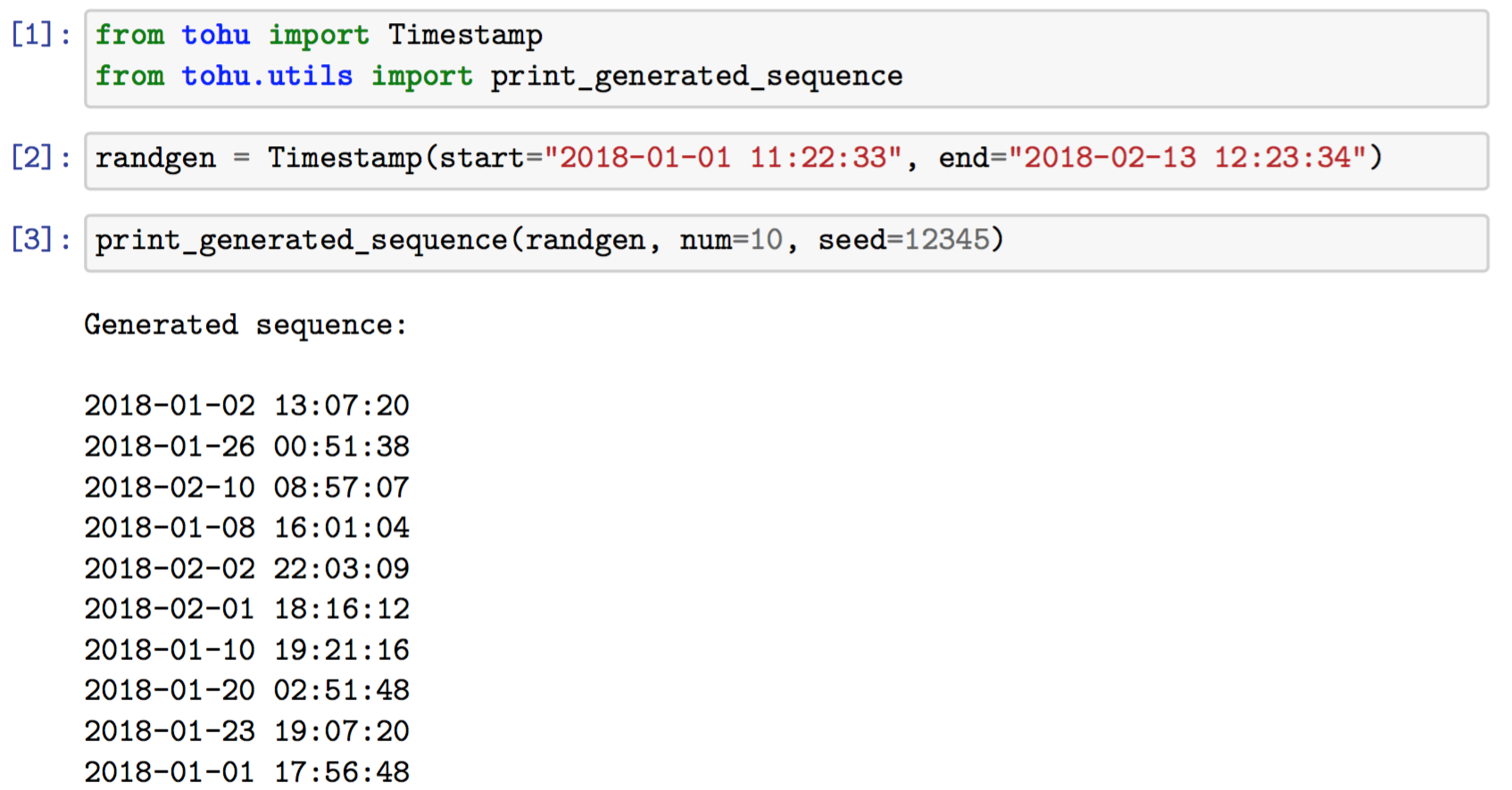
Figure 1: Excerpt from a Jupyter notebook which contains unit tests for tohu (a tool for reproducible generation of random synthetic data [1]). This example demonstrates how an nbval-tested Jupyter notebook can simultaneously serve as documentation for how to use the code, and at the same time serve as a unit test for the generated output (in the last cell). The command is generating a sequence of random dates and times between a given start and end time. This type of output is easy for a human to verify by inspection but inconvenient to copy and paste into a sequence of formal assert statements. In addition, if the output changes, it is trivial to update the Jupyter notebook-based test by re-executing the cells, whereas manual update of assert statements would be more laborious.

Secondly, not all researchers have training in software development [17], so they may not have been trained in writing tests, and may stick to manual checks because the overhead of writing formal tests may feel too much of a burden, especially if the design and interface is still changing and they are expected to be updated frequently. This provides an incentive to delay automatic testing until later in the project, or to never complete this.

Proponents of test-driven development (TDD) [3] advocate for writing tests upfront, before the actual implementation. This has multiple benefits: it gives a clear indication when the coding task for a given iteration is completed (namely, when all the tests pass); and it helps identify the interface requirements without getting caught up in the weeds of the implementation. On the other hand, the TDD approach can be impractical during prototyping, when one is trying to identify whether an approach is even feasible, or trying to find any implementation (which can then be discarded and re-implemented using a TDD approach).

A useful compromise is to use “explorative sprints” where one focuses purely on the exploratory aspects, and learns enough about the approaches and potential to then tackle the actual implementation. As soon as this sprint leads to an insight that is worth preserving one should be able to convert the notebook into a set of tests or documentation which helps freeze the desired behaviour in place. (This provides the reassurance that further changes or additions to the code will not break the current implementation.)

A useful analogue is that of a “ratchet wheel”, where each new nbval-tested notebook acts as an additional “latch” to prevent it from accidentally releasing and turning to undesired behaviour.

Nbval and notebooks can help convert those interactive and implicitly defined checks into more formal and automatically verifiable tests with minimal overhead, so they can be run regularly and automatically and ideally be included in continuous integration runs.

2.4 Producing (reproducible) research outputs

When the software has sufficiently matured that it can be used to produce outputs that are subsequently published in academic journals, and – for example – are used to drive healthcare, engineering or economic decisions and policy, it is important to ensure these outputs are reproducible: is all the required information provided with the publication/report so that another party could repeat the study, and get to the same conclusions?

Reproducibility is an important topic in its own right, and increasingly expected by funding bodies and publishers (for example [9]). The Jupyter Notebook is a useful tool to support this [20]: by driving computational science and data science from Jupyter notebooks, the notebooks serve as a detailed and complete transcript of all steps required to produce the results in the paper. The computational code used is typically kept in external libraries that are only called from the notebooks. A number of authors have started to publish (Github) repositories that complement publications, and provide one notebook per figure in the publication: by executing the notebook, the figure can be reproduced (for example [2]), and we endorse this as good practice.

With research codes, the underlying code may develop further, and this would break the reproducibility of the notebooks. The nbval requirement for this use case is to be able to automatically re-execute notebooks and to confirm that they produce the same results as stored, or alert to a problem by reporting a failure. Software solutions to address the problem when the code base changes are outside the scope of this paper; possibly solutions include versioning of the underlying code and/or to preserve the software environments as was used at time of publication.

2.5 Documenting software

2.5.1 Introduction

In order to share research with the world, it needs to be documented. The minimum documentation for research outputs is a complete description of all required steps to produce the research outputs (see section 2.4).

Sometimes the research software that has been used for a study has value in its own right: it may be re-usable for a follow up study, or even evolve into a framework that allows simulating / analysing many other systems, or can be developed further more effectively than recreating a new tool from scratch.

In that case, more documentation of the software is required: tutorials, how-to guides, contextual explanations and references (including application interface definitions) [8]).

Research software is likely to keep changing over time: These frequent changes can be a challenge for keeping documentation up-to-date, in particular if the people working on the software are so familiar with it that they rarely need to consult the documentation.

2.5.2 Use of Jupyter notebooks for documentation

The creation of software documentation using Jupyter notebooks can be very effective, combining descriptive text, equations, and code in the same notebook document [5, 22]. By executing the code cells, the output from the execution is inserted automatically into the document. For scientific purposes, figures and images created from commands is a common use case, and these are also inserted into the notebook [22] as an output. If a figure or a code segment needs updating, it is sufficient to change the code segment and to re-execute the cells.

If there are any changes to the software that is used and described in the notebook, the documentation can be updated by re-executing the notebook (as this will update the text-based and media outputs that are generated in the notebook). This partly automates updating of the documentation, and reduces manual effort.

Because notebooks can be used as sources for Sphinx [6, 15] and MkDocs [7, 16] documentation, any computational and data science data exploration can become a part of the documentation, and is often useful as a how-to guide or tutorial.

This documentation embedded in notebooks needs to be contrasted to the more conventional method of documentation generation, where descriptive text is stored in one document (for example in the restructuredtext or markdown format), which may include code segments that either need to be copied and pasted or included from a separate file. Inclusion of figure files is realised through a command that lists the name of the file containing the figure on disk, and inclusion of that file at a later documentation compile time. In this case, updating the code segment that leads to a figure requires manual transfer of the code snippet into an executable file/environment, and execution of this, and taking care to make sure the right figure file is updated as a result of this execution. Once this is done, the whole documentation needs to be compiled to check that the resulting html or pdf output is correct.

2.5.3 Executable “live” documentation

We mention in passing the possibility of executing Jupyter notebooks in the cloud using the Binder project and the mybinder.org instance [18]: Using this service, Jupyter notebook based documentation can be turned into executable documentation (as long as the software and data required are available on the Internet). The reader can jump into an executable notebook that is hosted on the remote machine of the mybinder service, and execute and modify examples from the documentation without having to install any software locally (only a web browser is required) [5]. This reduces the barrier towards learning a new piece of software. Binder is also useful for reproducible science [4].

2.5.4 Nbval for documentation

Assuming the documentation is created using Jupyter notebooks, a tool such as nbval can address some of the the documentation challenges: Nbval’s role is to help capturing anything that stops working, for example by using nbval as part of the continuous integration to check that the documentation notebooks execute and produce the output as expected.

This is helpful if the documentation is created up-front or alongside the development (in an iterative fashion) as it alerts the developers when new interfaces or behaviour make the documentation notebooks incorrect. It is also helpful when documentation is created at a particular point in the project’s lifecycle: it is typically not revisited by the authors (as they don’t need to consult the documentation) and without periodic testing of the documentation, it may become inaccurate when further development is taking place.

Using nbval to validate documentation as part of the continuous integration, will also alert the developers to changes in behaviour of third party libraries that are used in a given project.

2.5.5 Use of documentation as tests

An existing Jupyter notebook that documents or showcases the behaviour of a piece of software by showing code snippets together with the output values that the code produces, can also be seen as a set of software tests (see Fig. 1 for a simple example). If this is a low level piece of code, we can interpret this as a unit test, whereas if it tests features of a larger module or a combination of modules, it can be seen as a system test [23].

2.6 Requirements for nbval

Drived by these observations, we desired a tool that helps to keep Jupyter notebook based documents up-to-date, and that allows to read the combination of a code cell and the stored output as a regression test: can that same output be recomputed from the input? This should be done automatically, so that for each notebook cell, we have a PASS or FAIL outcome. This can then be integrated into existing unit test frameworks, and allow us to (i) use existing notebooks as automatic tests, and (ii) to check if existing documentation notebooks are still up-to-date. The tool NoteBook VALidate (nbval) has been developed to fulfil these requirements.

3 The nbval tool

We provide an overview of the nbval design and implementation, usage options, and comment on its limitations. The tool is available as open source [12] and more details are provided in the documentation [19].

3.1 A plugin to pytest

To re-use existing functionality as much as possible, we have developed the current version of nbval as a plugin to the pytest tool [21]. Pytest can scan subdirectory trees for files that match particular patterns. With the nbval plugin activated, pytest will find files with the extension .ipynb, and validate each of these notebooks.

The Jupyter notebook format .ipynb stores outputs and inputs for each cell. Validating the notebook means to rerun the notebook and to make sure that it generates the same outputs as have been stored. Fig. 2 shows example output from validating a notebook.

⬇

$ py.test --nbval -v 03-data-types-structures.ipynb

============================= test session starts =========

platform darwin -- Python 3.8.0, pytest-5.3.1, ...

plugins: nbval-0.9.3

collected 137 items

03-data-types-structures::ipynb::Cell 0 PASSED [ 0%]

03-data-types-structures::ipynb::Cell 1 PASSED [ 1%]

03-data-types-structures::ipynb::Cell 2 PASSED [ 2%]

...

03-data-types-structures::ipynb::Cell 136 PASSED [100%]

===================== 137 passed in 6.08s =================

Figure 2: Example output from running nbval to validate one Jupyter notebook: each code cell in the notebook becomes a test. The chosen example is chapter 3 of a book [10] which is composed of a sequence of Jupyter notebooks (one per chapter), and this nbval test is used as part of the continuous integration on Travis CI. The --nbval flag requests that pytest will process ipynb files. The -v requests more verbose output from pytest than is standard.

3.2 Usage

We use nbval by running pytest with the --nbval or --nbval-lax flag (the difference is described below). This causes pytest to collect files with a .ipynb extension and pass them to nbval, in addition to finding and running more conventional Python tests.

As a basic check, nbval expects all cells to run without errors. If executing a cell produces an error, it counts as a failure regardless of any output it produces. If a cell runs without an error, there are several ways to control whether its output should be checked.

3.3 Controlling output checks

Some code is meant to produce entirely consistent output given the same input. However, in many cases some output is expected to vary — e.g. if a timestamp is displayed, or if the code includes any random elements. Various features of nbval allow it to check only selected parts of the output.

There are two possible ways to approach this. In lax or relaxed mode (with the --nbval-lax option), no output is checked by default, but the author of the notebook can mark cells as described below to have their output checked. In strict mode (with the --nbval flag), all output is checked except for cells marked to indicate otherwise.

Lax mode provides a fairly quick way to validate notebooks written primarily as documentation, which will detect in many cases if code changes break the examples.

Using strict mode, it generally takes some work to make a notebook pass, as one needs to deal with any cells which may produce different output while still working correctly. The strict mode will also pick up subtle changes in the way output is produced. For example, if the text-based formatting of numpy arrays was to change by a space somewhere, the output cells displaying numpy arrays would fail. If a manual review of the failures shows that the change is not a problem, rerunning the notebook and saving the new output will make these tests pass in the future.

3.4 Cell markers

Code comments or cell tags can be used to enable or disable output checking cell-by-cell. Cell tags are a Jupyter feature, where short strings can be stored in the metadata of each cell. These are not visible by default, but a cell toolbar can be enabled to see and edit them.

Adding a tag nbval-check-output to a cell tells nbval to check its output in relaxed mode, while nbval-ignore-output disables output checking in strict mode. The same words can also be used as comments in the code, but here they are uppercase and separated by underscores, e.g.:

nbval also recognises some other markers specified in the same ways: nbval-skip will skip over a code cell entirely, and nbval-raises-exception or raises-exception will ignore an error from executing a cell, which would normally be shown as a failure.

3.5 Example for successful (PASS) and unsuccesful validation (FAIL)

A code cell containing deterministic code should pass. For example:

⬇

print(’Hello World’)

A notebook containing one cell that will create different output when executed again, will fail in strict mode. Figure LABEL:fig:fail-time shows output from a failing test for a code cell containing these lines:

⬇

import time

time.asctime()\end{lstlisting}

\begin{figure}[tb!]

\centering

\lstinputlisting[basicstyle=\ttfamily\scriptsize,frame=single]{time-short.txt}

\caption{An example for a mismatch in output, which is reported as a failure

when running \nbval{} in strict mode (using \texttt{--nbval}):

The timestamp saved is different from the timestamp when the cell was executed by \nbval.

The ‘‘\texttt{-}’’ sign before ‘‘Thu Dec 12 \ldots’’

indicates that this line of output is present in the saved output in file

\texttt{time.ipynb} but missing in the re-computed output, and

the \label{fig:fail-time} ‘‘\texttt{+}’’ sign two lines below indicates that

this line is new in the computed output and was not present in the saved file.

}

\end{figure}

\subsection{Sanitizing output with regular expressions}\label{regex-output-sanitizing}

\nbval{} supports more fine-grained handling of variable outputs,

by matching and sanitising patterns such as timestamps or memory addresses

within output that it is comparing.

The user can specify a sanitizing file at the command prompt

using the following flag:

\begin{lstlisting}[basicstyle=\footnotesize\ttfamily]

$ py.test --nbval x.ipynb --sanitize-with my_sanitize_file

This sanitize file my_sanitize_file contains a number of regular expressions and replacement strings. It is recommended to replace the removed output with a recognisable marker; for instance a timestamp like 16:44:06 might be replaced with TIMESTAMP. This replacement will be done in both the saved and the recomputed output before comparing them, so differences only in the replaced text do not cause failures. The marker is useful to understand failing tests.

3.6 Figures and multimedia elements

By default, only text output is compared [19], but nbval can integrate with nbdime [11] to display rich comparisons when outputs differ. If this option (--nbdime) is used, image outputs (PNG and JPEG formats) are also compared.

4 Summary

Nbval is a plugin to pytest, which allows to check that the output saved in the past in a notebook file is consistent with output computed today. Use cases include reproducible science, checks that deployed software behaves as its documentation suggests, that tutorials, manuals and textbooks remain up-to-date, and to help notice if support libraries change their behaviour. Deployment of nbval in continuous integration automates this process, and notebooks can serve as additional system tests and provide additional test coverage. We note that unit, integration and system tests can be written using Jupyter notebooks; which reduces the effort of formulating the test statement. Notebooks in combination with nbval and continuous integration can be used to develop documentation and tests as part of the design exploration and implementation phase in an agile manner.

Conceptionally, nbval provides testing functionality for notebooks which is similar to doctest for Python documentation strings. Due to the nature of notebooks, these can be used more flexibly than docstrings as outlined above.

4.0.1 Funding acknowledegments

We acknowledge support from the Horizon 2020 European Research Infrastructure project OpenDreamKit (676541) and Photon and Neutron Open Science Cloud (PaNOSC) project (823852), EPSRC’s Centre for Doctoral Training in Next Generation Computational Modelling (EP/L015382/1), EPSRC’s Doctoral Training Centre in Complex System Simulation (EP/G03690X/1), CONICYT Chilean scholarship programme Becas Chile (72140061), the Gordon and Betty Moore Foundation through Grant GBMF #4856, the Alfred P. Sloan Foundation and by the Helmsley Trust, the University of Southampton, Simula, and European XFEL.

References

- [1] Albert, M.: tohu: Your friendly synthetic data generator (2020), https://github.com/maxalbert/tohu
- [2] Albert, M., Fangohr, H., Metaxas, P.J.: Supplementary data and code for paper: ”frequency-based nanoparticle sensing over large field ranges using the ferromagnetic resonances of a magnetic nanodisc”. Nanotechnology (Aug 2016). https://doi.org/10.5281/zenodo.60605, https://github.com/maxalbert/paper-supplement-nanoparticle-sensing
- [3] Beck, K.: Test Driven Development. By Example (Addison-Wesley Signature). Addison-Wesley Longman, Amsterdam (2002)
- [4] Beg, M., Fangohr, H.: Reproducible micromagnetics (2019), https://github.com/reproducible-micromagnetics
- [5] Beg, M. et al: Discretisedfield documentation using jupyter notebooks (2020), https://discretisedfield.readthedocs.io
- [6] Brandl, G. et al: Sphinx 2.3.0 (2019), http://www.sphinx-doc.org/
- [7] Christie, T. and Matthews, D. and Limberg, W.: Mkdocs 1.0.4 (2018), https://www.mkdocs.org/
- [8] Daniele Procida: What nobody tells you about documentation (2017), https://www.divio.com/blog/documentation/
- [9] Editor: Announcement: Towards greater reproducibility for life-sciences research in nature. Journal (2017). https://doi.org/10.1038/546008a
- [10] Fangohr, H.: Introduction to Python for computational science and engineering (2019). https://doi.org/10.5281/ZENODO.1411868, https://github.com/fangohr/introduction-to-python-for-computational-science-and-engineering
- [11] Fauske, V. et al: nbdime 1.1.0 (2019), https://github.com/jupyter/nbdime/
- [12] Fauske, V. et al: Nbval (2020), http://github.com/computationalmodelling/nbval
- [13] Feathers, M.: Working Effectively with Legacy Code. Prentice Hall PTR, USA (2004)
- [14] Fowler, M.: Refactoring: Improving the Design of Existing Code. Addison-Wesley Longman Publishing Co., Inc., USA (1999)
- [15] Geier, M. et al: nbsphinx 0.5.0 (2019), https://github.com/spatialaudio/nbsphinx
- [16] Gray, J.: mknotebooks 0.1.7 (2019), https://github.com/greenape/mknotebooks
- [17] Hettrick, S.: (2014), https://www.software.ac.uk/blog/2014-12-04-its-impossible-conduct-research-without-software-say-7-out-10-uk-researchers
- [18] Jupyter et al: Binder 2.0 - reproducible, interactive, sharable environments for science at scale. In: Proceedings of the 17th Python in Science Conference. pp. 113 – 120 (2018). https://doi.org/10.25080/Majora-4af1f417-011, http://mybinder.org
- [19] Jupyter et al: NBVAL documentation on readthedocs.org (2020), https://nbval.readthedocs.io
- [20] Kluyver, T. et al: Jupyter notebooks – a publishing format for reproducible computational workflows. In: Loizides, F., Schmidt, B. (eds.) Positioning and Power in Academic Publishing: Players, Agents and Agendas. pp. 87 – 90. IOS Press (2016), http://jupyter.org
- [21] Krekel, H., Oliveira, B., Pfannschmidt, R., Bruynooghe, F., Laugher, B., Bruhin, F.: pytest 3.7 (2004), https://github.com/pytest-dev/pytest
- [22] Pandas team: Pandas documentation using Jupyter notebooks (2020), https://pandas.pydata.org/pandas-docs/version/0.15/visualization.html
- [23] van Vliet, H.: Software Engineering Principles and Practice. Jon Wiley & Sons, third edn. (2008)