Theory status and implications of $R_{K}^{(\ast)}$

Abstract:

The LHCb and Belle collaborations have reported on some anomalies in $b\to s$ transitions, with discrepancies with the Standard Model predictions in some angular observables and branching ratios and intriguing hints for lepton universality violation. We will review the current situation and explore the proposed New Physics explanations for these tensions. We will also discuss the possible connection of the $b\to s$ anomalies to other central problems in physics, such as the dark matter of the Universe, the origin of neutrino masses or the strong CP problem.

1 Introduction

Since 2013, B physics has attracted a great deal of attention in the particle physics community due to a wide set of intriguing experimental anomalies. In particular, several measurements in semileptonic processes involving $b\to s$ transitions have been found to deviate from the Standard Model (SM) predicted values, hence suggesting the presence of some New Physics (NP) effects. The list of anomalies includes substantial deviations in the measurements of branching ratios and angular observables by the LHCb [1, 2, 3, 4] and Belle [5, 6] collaborations, as well as discrepancies in the observables

$$R_{K^{(\ast)}}=\frac{\Gamma(B\rightarrow K^{(\ast)}\mu^{+}\mu^{-})}{\Gamma(B\rightarrow K^{(\ast)}e^{+}e^{-})}\,,$$ (1)

measured in specific dilepton invariant mass squared ranges $q^{2}\in[q^{2}_{\rm min},q^{2}_{\rm max}]$. The $R_{K^{(\ast)}}$ ratios were introduced in [7] in order to test lepton flavor universality (LFU), a central feature of the SM that predicts $R_{K^{(\ast)}}\sim 1$. Very interestingly, the LHCb results for the $R_{K}$ ratio in one $q^{2}$ bin [8, 9] and the $R_{K^{\ast}}$ ratio in two $q^{2}$ bins [10] were found to lie significantly below one:

$$R_{K} =0.846^{+0.060}_{-0.054}\text{(stat)}^{+0.016}_{-0.014}\text{(syst)}\,,\quad q^{2}\in[1,6]~{}\text{GeV}^{2}\,,$$

$$R_{K^{\ast}} =0.660^{+0.110}_{-0.070}\text{(stat)}\pm 0.024\text{(syst)}\,,\quad q^{2}\in[0.045,1.1]~{}\text{GeV}^{2}\,,$$

$$R_{K^{\ast}} =0.685^{+0.113}_{-0.069}\text{(stat)}\pm 0.047\text{(syst)}\,,\quad q^{2}\in[1.1,6.0]~{}\text{GeV}^{2}\,.$$ (2)

A comparison between the LHCb results and the SM predictions for $R_{K}$ and $R_{K^{\ast}}$ derived in [11, 12] leads to discrepancies with the SM above the $2\,\sigma$ level, with the precise statistical significance depending on the dilepton invariant mass squared range considered. Furthermore, it is generally accepted that unknown QCD effects cannot account for the observed deviations, since they cancel out to great accuracy in the $R_{K^{(\ast)}}$ ratios. Although these hints are still not very significant, they are definitely intriguing and, if confirmed, would have dramatic consequences for the shape of NP, which would necessarily violate LFU.

Many NP models have been proposed in order to explain the $b\to s$ anomalies. The most widely studied scenarios include heavy $Z^{\prime}$ bosons or leptoquarks, although many other possibilities and variations of the minimal setups have also been put forward in recent years. Here we discuss the most popular options and discuss their possible connection to other open problems in physics. Although we will not attempt to make a complete review of all the proposed scenarios, and many well-motivated models will be omitted, we hope that our discussion constitutes a good description of the panorama depicted by the model builders.

2 Interpreting the anomalies

The set of experimental measurements in $b\to s$ transitions can be interpreted in a model-independent way by using the language of Effective Field Theory (EFT). This approach is valid if all NP degrees of freedom have masses well above the energy scale of the observables of interest, a well-motivated assumption due to the lack of observations in direct searches, both at the Large Hadron Collider (LHC) as well as in low-energy experiments. In this case, one can integrate out all the NP states and describe the physical observables by a collection of non-renormalizable operators, with canonical dimensions higher than four.

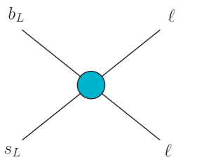
Figure 1: $O_{9}$ operator with muon lepton flavors.

The effective Hamiltonian describing $b\to s$ transitions is typically written as

$$\mathcal{H}_{\text{eff}}=-\frac{4G_{F}}{\sqrt{2}}\,V_{tb}V_{ts}^{\ast}\,\frac{e^{2}}{16\pi^{2}}\,\sum_{i}\left(C_{i}\,\mathcal{O}_{i}+C^{\prime}_{i}\,\mathcal{O}^{\prime}_{i}\right)+\text{h.c.}\,,$$ (3)

where $G_{F}$ denotes the Fermi constant that sets the strength of weak interactions, $e$ is the electric charge and $V$ the Cabibbo-Kobayashi-Maskawa (CKM) matrix. $\mathcal{O}_{i}$ and $\mathcal{O}^{\prime}_{i}$ are dimension-6 effective operators contributing to $b\to s$ quark flavor transitions, while $C_{i}$ and $C^{\prime}_{i}$ are their Wilson coefficients. Among all possible operators involved in $b\to s$ semileptonic decays, the following subset turns out to be relevant for the interpretation of the $b\to s$ anomalies:

$$\mathcal{O}_{7} =\left(\bar{s}\sigma_{\mu\nu}P_{R}b\right)\,F^{\mu\nu}\,, \mathcal{O}^{\prime}_{7} =\left(\bar{s}\sigma_{\mu\nu}P_{L}b\right)\,F^{\mu\nu}\,,$$ (4)

$$\mathcal{O}_{9} =\left(\bar{s}\gamma_{\mu}P_{L}b\right)\,\left(\bar{\ell}\gamma^{\mu}\ell\right)\,, \mathcal{O}^{\prime}_{9} =\left(\bar{s}\gamma_{\mu}P_{R}b\right)\,\left(\bar{\ell}\gamma^{\mu}\ell\right)\,,$$ (5)

$$\mathcal{O}_{10} =\left(\bar{s}\gamma_{\mu}P_{L}b\right)\,\left(\bar{\ell}\gamma^{\mu}\gamma_{5}\ell\right)\,, \mathcal{O}^{\prime}_{10} =\left(\bar{s}\gamma_{\mu}P_{R}b\right)\,\left(\bar{\ell}\gamma^{\mu}\gamma_{5}\ell\right)\,.$$ (6)

Here $\ell=e,\mu,\tau$ denotes the lepton flavor. Although the operators and Wilson coefficients actually have flavor indices, we will omit them in order to simplify the notation. A diagrammatric representation of a muonic $O_{9}$ operator is provided in Fig. 1. It is common to split the Wilson coefficients in two pieces: the SM contributions and the NP contributions, defining

$$C_{7} =C_{7}^{\text{SM}}+C_{7}^{\text{NP}}\,,$$ (7)

$$C_{9} =C_{9}^{\text{SM}}+C_{9}^{\text{NP}}\,,$$ (8)

$$C_{10} =C_{10}^{\text{SM}}+C_{10}^{\text{NP}}\,.$$ (9)

In principle, analogous splittings can be defined for the primed coefficients, but in this case the SM contributions are rather small and therefore one simply has $C^{\prime}_{7}\simeq C^{\prime\>\text{NP}}_{7}$, $C^{\prime}_{9}\simeq C^{\prime\>\text{NP}}_{9}$ and $C^{\prime}_{10}\simeq C^{\prime\>\text{NP}}_{10}$. The SM contributions are calculable [13], while the NP contributions remain as free parameters to be determined. The observables measured by the experimental collaborations can be written in terms of the $C_{i}$ and $C^{\prime}_{i}$ Wilson coefficients. For instance, simple expressions for $R_{K}$ and $R_{K^{\ast}}$ can be found in [14]. Since the same Wilson coefficients enter several observables, one expects a pattern of deviations from the SM, rather than a single anomaly in a specific observable. The strategy to exploit this fact is therefore clear: the NP contributions can be determined with a global fit of the observables to experimental data.

Several groups [15, 16, 17, 18, 19, 20, 21, 22] have followed this strategy. The different fits agree qualitatively, although they differ quantitatively due to differences in the form factors, the treatment of uncertainties or the computational techniques used. In all cases, a NP scenario with one or more NP contributions to the Wilson coefficients is preferred over the pure SM scenario. In all fits, the muonic $C_{9}$ coefficient seems to be crucial. A good fit to data is obtained with a NP contribution to this coefficient of about 20% of the SM contribution (and with opposite sign). Other muonic coefficients may have NP contributions as well and in fact three competitive 1D (muonic) scenarios emerge: $C_{9}^{\text{NP}}$ only, $C_{9}^{\text{NP}}=-C_{10}^{\text{NP}}$ and $C_{9}^{\text{NP}}=-C_{9}^{\prime\>\text{NP}}$. No indication for NP contributions in electronic coefficients is found. 

These findings provide a quantitive assessment of the $b\to s$ anomalies and serve as a guide for model builders that aim at an explanation. For instance, valuable information about the scale of NP can be inferred [23]. $C_{9}^{\text{NP}}\sim-20\%\,\times\,C_{9}^{\text{SM}}$ leads to

$$\frac{C_{9}^{\rm NP}}{\Lambda_{\rm NP}^{2}}\,\sim 20\%\,\times\,\frac{4G_{F}}{\sqrt{2}}\,V_{tb}V_{ts}^{\ast}\,\frac{e^{2}}{16\pi^{2}}\,C_{9}^{\rm SM}\,.$$ (10)

One can then estimate the scale of NP, $\Lambda_{\rm NP}$, in several generic scenarios:

• Unsuppressed NP: $\displaystyle\quad C_{9}^{\rm NP}=1\quad\Rightarrow\quad\Lambda_{\rm NP}\sim 30$ TeV.

• CKM-suppressed NP: $\displaystyle\quad C_{9}^{\rm NP}=|V_{tb}V_{ts}^{\ast}|\quad\Rightarrow\quad\Lambda_{\rm NP}\sim 6$ TeV.

• Loop-suppressed NP: $\displaystyle\quad C_{9}^{\rm NP}=\frac{1}{16\pi^{2}}\quad\Rightarrow\quad\Lambda_{\rm NP}\sim 2.50$ TeV.

• CKM&loop-suppressed NP: $\displaystyle\quad C_{9}^{\rm NP}=\frac{|V_{tb}V_{ts}^{\ast}|}{16\pi^{2}}\quad\Rightarrow\quad\Lambda_{\rm NP}\sim 0.5$ TeV.

This way, one concludes that only when the NP effects are suppressed (by CKM factors and/or loops), the scale of NP is low enough to be probed directly at current facilities. In what concerns the NP mediators behind the $O_{i}$ operators, only two possibilities exist at tree-level: a neutral $Z^{\prime}$ vector boson and a scalar or vector leptoquark. In fact, these have been the most popular options in the literature. Other possibilities at loop level have also been considered. We now proceed to discuss several example models aiming at an explanation to the $b\to s$ anomalies.

3 Models for $R_{K}^{(*)}$

The $b\to s$ anomalies have triggered the creativity of model builders and the construction of many new data-driven models. Some of these models would have never been built in the absence of the strong motivation emerged from the intriguing experimental hints in B-meson decays, which have opened new directions beyond the SM. Therefore, even if the anomalies go away, the model building community has found novel ways to address some of the most important problems in the SM and shed light on some of the crucial questions, such as the flavor problem, the dark matter of the Universe or the origin of neutrino masses.

We will now review some of the most popular setups proposed to explain the $b\to s$ anomalies.

3.1 $Z^{\prime}$ models

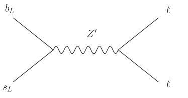
Figure 2: Generation of the $O_{9}$ operator due to the exchange of a neutral $Z^{\prime}$ vector boson.

$Z^{\prime}$ models argueably constitute the easiest solution to the $b\to s$ anomalies. A neutral $Z^{\prime}$ boson can generate the $O_{9}$ operator (and perhaps $O_{10}$ or $O_{9}^{\prime}$ as well) as shown in Fig. 2. The list of requirements for the model is rather short: a $Z^{\prime}$ boson that contributes to the desired operators, with flavor violating couplings to quarks and non-universal couplings to leptons.  Such vector boson would obtain its mass from the spontaneous breaking of an enlarged gauge symmetry group $\mathcal{G}$, which includes the SM gauge group $\mathcal{G}_{\rm SM}=\rm{SU(3)_{c}\times SU(2)_{L}\times U(1)_{Y}}$ as a subgroup and gets broken at the high-energy scale $\Lambda_{\rm NP}\sim m_{Z^{\prime}}$. The simplest solution is to add a new $\rm U(1)$ factor to the SM gauge group, but other more involved possibilities also exist.  Regarding the non-universal couplings to the SM charged leptons, one can broadly classify all $Z^{\prime}$ models in two categories:

• Direct models: in these models the $Z^{\prime}$ boson couples directly to the SM charged leptons, and therefore these must be charged non-universally under $\mathcal{G}$.

• Indirect models: in these models the SM charged leptons are universally charged under $\mathcal{G}$, and the non-universality is induced by their mixing with new fermionic states which have a different representation under $\mathcal{G}$.

Field	Spin	$\rm SU(3)_{c}\times\,SU(2)_{L}\times\,U(1)_{Y}\times U(1)_{X}$
$\phi$	$0$	$({\bf 1},{\bf 1},0,2)$
$Q_{L,R}$	$\frac{1}{2}$	$({\bf 3},{\bf 2},\frac{1}{6},2)$
$L_{L,R}$	$\frac{1}{2}$	$({\bf 1},{\bf 2},-\frac{1}{2},2)$

Table 1: New scalars and fermions in the model of [26].

Let us illustrate the category of indirect models with the setup introduced in [26]. The model extends $\mathcal{G}_{\rm SM}$ with a new $\rm U(1)_{X}$ factor, under which all the SM particles are singlets. The particle content of the model includes the new scalar $\phi$ as well as the new vector-like fermions $Q$ and $L$, charged under $\rm U(1)_{X}$.  We note that $\phi$ is a singlet of $\mathcal{G}_{\rm SM}$, while $Q$ and $L$ have the same representation under $\mathcal{G}_{\rm SM}$ as the SM quark and lepton doublets $q$ and $\ell$. Due to their vector-like nature, one can write gauge-invariant Dirac mass terms for $Q$ and $L$,

$$\mathcal{L}_{m}=m_{Q}\,\overline{Q}Q+m_{L}\,\overline{L}L\,.$$ (11)

Furthermore, they also have Yukawa interactions

$$\mathcal{L}_{Y}=\lambda_{Q}\,\overline{Q_{R}}\,\phi\,q_{L}+\lambda_{L}\,\overline{L_{R}}\,\phi\,\ell_{L}+\text{h.c.}\,.$$ (12)

Here $\lambda_{Q}$ and $\lambda_{L}$ are $3$-component Yukawa vectors. In what concerns the scalar sector, we will simply assume that the SM gauge symmetry is broken as usual and that $\phi$ gets the vacuum expectation value

$$\langle\phi\rangle=\frac{v_{\phi}}{\sqrt{2}}\,,$$ (13)

hence breaking the new $\rm U(1)_{X}$ piece and leading to a massive $Z^{\prime}$ boson, with mass $m_{Z^{\prime}}=2g_{X}v_{\phi}$, with $g_{X}$ the $\rm U(1)_{X}$ gauge coupling.

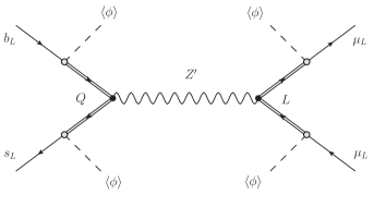
Figure 3: Generation of $O_{9}$ and $O_{10}$ in the model of [26]. Since the $Z^{\prime}$ couplings to fermions are purely left-handed, this model predicts $C_{9}^{\rm NP}=-C_{10}^{\rm NP}$.

Let us now come to the $b\to s$ anomalies and their resolution in this model. One should note that in this model the SM fermions do not couple directly to the $Z^{\prime}$ boson. These couplings are only generated after symmetry breaking due to the mixing with the vector-like fermions. This effectively leads to the generation of $O_{9}$ and $O_{10}$, as shown in Fig. 3. The non-universality in the charged lepton couplings to the $Z^{\prime}$ boson originates simply from the non-universality of the $\lambda_{L}$ Yukawa couplings. For instance, assuming $\lambda_{L}^{e}=\lambda_{L}^{\tau}=0$, the $Z^{\prime}$ boson couples to muons only, easily explaining the anomalies in $R_{K}$ and $R_{K^{\ast}}$.

Many direct models also exist, in some cases in combination with indirect couplings in the quark or lepton sectors. A very popular model is the one based on the $L_{\mu}-L_{\tau}$ gauge symmetry, pioneered in the context of the $b\to s$ anomalies in the relevant paper [28] and later explored in many other works. An extension of the $L_{\mu}-L_{\tau}$ gauge group to include the quark sector was considered in [29]. Other possibilities have also been discussed in the literature. For instance, the gauged BGL symmetry [30] introduced in [31] and the $\rm U(2)$ flavor symmetry in [32], to mention two particularly attractive proposals.

A generally very relevant constraint in all $Z^{\prime}$ models for the $b\to s$ anomalies is $B_{s}-\overline{B_{s}}$ mixing, recently discussed in detail in [33]. The potential conflict originates from the fact that this mixing is induced at tree-level and depends on the same $Z^{\prime}-b-s$ coupling required to explain the anomalies. In models with both left- and right-handed $Z^{\prime}$ couplings to quarks, one can in principle get a cancellation that alleviates the tension [34], but in models with only one chirality this is not possible [27]. In such cases, the usual solution is to suppress the $Z^{\prime}-b-s$ coupling at the cost of increasing the $Z^{\prime}-\mu-\mu$ coupling, so that the NP contributions to the muonic $C_{9}$ coefficients are large enough to explain the anomalies.

3.2 Leptoquark models

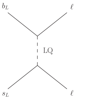
Figure 4: Generation of the $O_{9}$ operator due to the exchange of a leptoquark. The leptoquark can be either scalar or vector.

Leptoquarks [35] are scalars or vectors that couple simultaneously to both quarks and leptons. While they appear naturally in grand unified theories, there is in principle no fundamental reason why they cannot have masses well below the unification scale and have sizable effects in flavor observables. In fact, leptoquark models are also very popular and many simple solutions to the $b\to s$ anomalies have been proposed.  Fig. 4 shows how to generate the $O_{9}$ operator via the tree-level exchange of a leptoquark.

Leptoquarks have been widely discussed recently due to their potential to explain the experimental anomalies observed not only in neutral $b\to s$ transitions, the subject here, but also in charged $b\to c$ decays. We refer to other contributions to these conference proceedings where the phenomenology of leptoquarks and their role in solving the $b\to c$ anomalies are discussed in great detail. 

3.3 Loop models

Finally, loop models explain the $b\to s$ anomalies by generating the $O_{9}$ operator at loop level. Although this allows for a wider variety of options, since many possibilities for the particles running in the loop exist, fewer models with this feature have been built. The different one-loop models that one can construct in connection to the $b\to s$ anomalies have been classified in [36, 37]. Interestingly, the constraints from $B_{s}-\overline{B_{s}}$ mixing, so important in case of $Z^{\prime}$ models, can be very different depending on the charges chosen for the new states running in the loop. Also, as we will discuss below, some of the possible loop models include particles with the correct quantum numbers to be valid dark matter candidates, a possibility that has been explored in some works.

4 Connection to other physics problems

All models addressing the $b\to s$ anomalies include additional fields and, in some cases, new gauge symmetries. This offers many new phenomenological opportunities, as one would expect that the new states communicate not only to the sector strictly related to the anomalies, but also to other SM sectors. The natural question is then: what if the explanation to the $b\to s$ anomalies also solves other physics problems? In this Section we briefly discuss some of the ideas that have been presented in this direction, linking the $b\to s$ anomalies to dark matter, the origin of neutrino masses and the strong CP problem.

4.1 Dark matter

The possible link between the $b\to s$ anomalies and the dark matter of the Universe was reviewed in [38]. Here we will briefly discuss two representative examples.

Let us first consider the addition of the complex scalar $\chi$ to the model discussed in Sec. 3.1, with representation $({\bf 1},{\bf 1},0,-1)$ under the extended gauge group. This was actually the original version of the model introduced in [26]. Assuming that $\chi$ does not get a vacuum expectation value, the spontaneous breaking of the $\rm U(1)_{X}$ symmetry leaves a remnant $\mathbb{Z}_{2}$ dark parity, under which $\chi$ is odd and the rest of states are even. Therefore, $\chi$ is perfectly stable, without any additional ad-hoc symmetry. The same gauge symmetry behind the dynamics required to explain the $b\to s$ anomalies stabilizes the dark matter candidate.  Furthermore, $\chi$ is a singlet under the SM gauge group and does not have any Yukawa interaction. Assuming that the Higgs portal $|H|^{2}|\chi|^{2}$ term is suppressed, it can only be produced in the early Universe via $Z^{\prime}$ exchange. This establishes another link to the $b\to s$ anomalies. Ref. [26] shows that one can explain the anomalies in a region of the parameter space that can also reproduce the observed dark matter relic density.

A second example was provided in [42]. In this case a loop model for the $b\to s$ anomalies was considered. The particle content and gauge charges of the model is the same as in the model discussed in Sec. 3.1, but with a crucial difference: the $\rm U(1)_{X}$ symmetry is assumed to be global and conserved. Therefore, the $b\to s$ anomalies cannot be explained via $Z^{\prime}$ exchange, but the $O_{9}$ and $O_{10}$ operators are generated at the one-loop level, also with $C_{9}^{\rm NP}=-C_{10}^{\rm NP}$. Regarding dark matter, the conservation of $\rm U(1)_{X}$ stabilizes the lightest particle charged under this symmetry, and this is taken to be the scalar $\phi$. Again, the authors of [42] explicitly show that one can simultaneously explain the $b\to s$ anomalies and reproduce the measured dark matter relic density. Finally, the model is found to be testable in future direct DM detection experiments as well as by direct LHC searches.

4.2 Neutrino masses

The main open question in the lepton sector is the origin of neutrino masses. What if the $R_{K}$ and $R_{K^{\ast}}$ LFU violating hints (remember: L stands for lepton!) can guide us towards solving this central problem? While this seems like a very natural question, it has been explored very little in recent years.

Leptoquarks are familiar states in the neutrino mass model-building community. It is well known that the addition of two leptoquarks (or a leptoquark and another exotic state) allows one to induce radiative Majorana neutrino masses [43], and this mechanism has been considered in several leptoquark models for the B-anomalies [44, 45, 46]. Furthermore, the possible link between the violation of LFU and mixing in the leptonic sector has been discussed in [47, 48].

4.3 Strong CP problem

Many of the models capable to address all the experimental anomalies in B-meson decays, both in neutral $b\to s$ and in charged $b\to c$ transitions, include the $U_{1}\sim({\bf 3},{\bf 1},2/3)$ vector leptoquark.  This state has been shown to provide a good simultaneous explanation, but it also requires to extend the SM gauge group in order to embed $U_{1}$ as one of the gauge bosons. This has led to the so-called 4321 models, based on the extended gauge group $\mathcal{G}_{4321}\equiv\rm SU(4)\times SU(3)^{\prime}\times SU(2)_{L}\times U(1)^{\prime}$ [50, 51]. A remarkable feature of these models is that QCD emerges at low energies from the product of two non-Abelian gauge groups: $\mathrm{SU(3)_{c}}=\left[\mathrm{SU(3)_{4}\times SU(3)^{\prime}}\right]_{\rm diag}$, where $\rm SU(3)_{4}$ is a subgroup of $\rm SU(4)$. As shown in [52], the resolution of the strong CP problem à la Peccei-Quinn requires in this case the introduction of two axions. While the properties of the lightest one are those of the standard QCD axion, a second heavier axion must exist, with its mass and couplings closely related to the B-anomalies.

5 Summary

We are living exciting times in the flavor community, with the anomalies in B-meson decays providing a strong motivation for novel research in various directions. Here we have reviewed the current situation and discussed the different types of models proposed to address the anomalies in $b\to s$ transitions. We have also pointed out that $R_{K}$ and $R_{K^{\ast}}$ might just be the tip of the iceberg, with a whole NP sector close to be found, with potential impact in other central physics problems, such as the dark matter of the Universe, the origin of neutrino masses or the strong CP problem.

References

- [1] R. Aaij et al. [LHCb Collaboration], JHEP 1307 (2013) 084 doi:10.1007/JHEP07(2013)084 [arXiv:1305.2168 [hep-ex]].
- [2] R. Aaij et al. [LHCb Collaboration], Phys. Rev. Lett. 111 (2013) 191801 doi:10.1103/PhysRevLett.111.191801 [arXiv:1308.1707 [hep-ex]].
- [3] R. Aaij et al. [LHCb Collaboration], JHEP 1602 (2016) 104 doi:10.1007/JHEP02(2016)104 [arXiv:1512.04442 [hep-ex]].
- [4] R. Aaij et al. [LHCb Collaboration], JHEP 1509 (2015) 179 doi:10.1007/JHEP09(2015)179 [arXiv:1506.08777 [hep-ex]].
- [5] A. Abdesselam et al. [Belle Collaboration], arXiv:1604.04042 [hep-ex].
- [6] S. Wehle et al. [Belle Collaboration], Phys. Rev. Lett. 118 (2017) no.11, 111801 doi:10.1103/PhysRevLett.118.111801 [arXiv:1612.05014 [hep-ex]].
- [7] G. Hiller and F. Kruger, Phys. Rev. D 69 (2004) 074020 doi:10.1103/PhysRevD.69.074020 [hep-ph/0310219].
- [8] R. Aaij et al. [LHCb Collaboration], Phys. Rev. Lett. 113 (2014) 151601 doi:10.1103/PhysRevLett.113.151601 [arXiv:1406.6482 [hep-ex]].
- [9] R. Aaij et al. [LHCb Collaboration], Phys. Rev. Lett. 122 (2019) no.19, 191801 doi:10.1103/PhysRevLett.122.191801 [arXiv:1903.09252 [hep-ex]].
- [10] R. Aaij et al. [LHCb Collaboration], JHEP 1708 (2017) 055 doi:10.1007/JHEP08(2017)055 [arXiv:1705.05802 [hep-ex]].
- [11] S. Descotes-Genon, L. Hofer, J. Matias and J. Virto, JHEP 1606 (2016) 092 doi:10.1007/JHEP06(2016)092 [arXiv:1510.04239 [hep-ph]].
- [12] M. Bordone, G. Isidori and A. Pattori, Eur. Phys. J. C 76 (2016) no.8, 440 doi:10.1140/epjc/s10052-016-4274-7 [arXiv:1605.07633 [hep-ph]].
- [13] S. Descotes-Genon, T. Hurth, J. Matias and J. Virto, JHEP 1305 (2013) 137 doi:10.1007/JHEP05(2013)137 [arXiv:1303.5794 [hep-ph]].
- [14] A. Celis, J. Fuentes-Martin, A. Vicente and J. Virto, Phys. Rev. D 96 (2017) no.3, 035026 doi:10.1103/PhysRevD.96.035026 [arXiv:1704.05672 [hep-ph]].
- [15] M. Algueró, B. Capdevila, A. Crivellin, S. Descotes-Genon, P. Masjuan, J. Matias and J. Virto, Eur. Phys. J. C 79 (2019) no.8, 714 doi:10.1140/epjc/s10052-019-7216-3 [arXiv:1903.09578 [hep-ph]].
- [16] A. K. Alok, A. Dighe, S. Gangal and D. Kumar, JHEP 1906 (2019) 089 doi:10.1007/JHEP06(2019)089 [arXiv:1903.09617 [hep-ph]].
- [17] M. Ciuchini, A. M. Coutinho, M. Fedele, E. Franco, A. Paul, L. Silvestrini and M. Valli, Eur. Phys. J. C 79 (2019) no.8, 719 doi:10.1140/epjc/s10052-019-7210-9 [arXiv:1903.09632 [hep-ph]].
- [18] G. D’Amico, M. Nardecchia, P. Panci, F. Sannino, A. Strumia, R. Torre and A. Urbano, JHEP 1709 (2017) 010 doi:10.1007/JHEP09(2017)010 [arXiv:1704.05438 [hep-ph]].
- [19] A. Datta, J. Kumar and D. London, Phys. Lett. B 797 (2019) 134858 doi:10.1016/j.physletb.2019.134858 [arXiv:1903.10086 [hep-ph]].
- [20] J. Aebischer, W. Altmannshofer, D. Guadagnoli, M. Reboud, P. Stangl and D. M. Straub, arXiv:1903.10434 [hep-ph].
- [21] K. Kowalska, D. Kumar and E. M. Sessolo, Eur. Phys. J. C 79 (2019) no.10, 840 doi:10.1140/epjc/s10052-019-7330-2 [arXiv:1903.10932 [hep-ph]].
- [22] A. Arbey, T. Hurth, F. Mahmoudi, D. M. Santos and S. Neshatpour, Phys. Rev. D 100 (2019) no.1, 015045 doi:10.1103/PhysRevD.100.015045 [arXiv:1904.08399 [hep-ph]].
- [23] L. Di Luzio and M. Nardecchia, Eur. Phys. J. C 77 (2017) no.8, 536 doi:10.1140/epjc/s10052-017-5118-9 [arXiv:1706.01868 [hep-ph]].
- [24] S. M. Boucenna, A. Celis, J. Fuentes-Martin, A. Vicente and J. Virto, Phys. Lett. B 760 (2016) 214 doi:10.1016/j.physletb.2016.06.067 [arXiv:1604.03088 [hep-ph]].
- [25] S. M. Boucenna, A. Celis, J. Fuentes-Martin, A. Vicente and J. Virto, JHEP 1612 (2016) 059 doi:10.1007/JHEP12(2016)059 [arXiv:1608.01349 [hep-ph]].
- [26] D. Aristizabal Sierra, F. Staub and A. Vicente, Phys. Rev. D 92 (2015) no.1, 015001 doi:10.1103/PhysRevD.92.015001 [arXiv:1503.06077 [hep-ph]].
- [27] P. Rocha-Moran and A. Vicente, Phys. Rev. D 99 (2019) no.3, 035016 doi:10.1103/PhysRevD.99.035016 [arXiv:1810.02135 [hep-ph]].
- [28] W. Altmannshofer, S. Gori, M. Pospelov and I. Yavin, Phys. Rev. D 89 (2014) 095033 doi:10.1103/PhysRevD.89.095033 [arXiv:1403.1269 [hep-ph]].
- [29] A. Crivellin, G. D’Ambrosio and J. Heeck, Phys. Rev. D 91 (2015) no.7, 075006 doi:10.1103/PhysRevD.91.075006 [arXiv:1503.03477 [hep-ph]].
- [30] G. C. Branco, W. Grimus and L. Lavoura, Phys. Lett. B 380 (1996) 119 doi:10.1016/0370-2693(96)00494-7 [hep-ph/9601383].
- [31] A. Celis, J. Fuentes-Martin, M. Jung and H. Serodio, Phys. Rev. D 92 (2015) no.1, 015007 doi:10.1103/PhysRevD.92.015007 [arXiv:1505.03079 [hep-ph]].
- [32] A. Falkowski, M. Nardecchia and R. Ziegler, JHEP 1511 (2015) 173 doi:10.1007/JHEP11(2015)173 [arXiv:1509.01249 [hep-ph]].
- [33] L. Di Luzio, M. Kirk, A. Lenz and T. Rauh, JHEP 1912 (2019) 009 doi:10.1007/JHEP12(2019)009 [arXiv:1909.11087 [hep-ph]].
- [34] A. Crivellin, L. Hofer, J. Matias, U. Nierste, S. Pokorski and J. Rosiek, Phys. Rev. D 92 (2015) no.5, 054013 doi:10.1103/PhysRevD.92.054013 [arXiv:1504.07928 [hep-ph]].
- [35] I. Doršner, S. Fajfer, A. Greljo, J. F. Kamenik and N. Košnik, Phys. Rept. 641 (2016) 1 doi:10.1016/j.physrep.2016.06.001 [arXiv:1603.04993 [hep-ph]].
- [36] B. Gripaios, M. Nardecchia and S. A. Renner, JHEP 1606 (2016) 083 doi:10.1007/JHEP06(2016)083 [arXiv:1509.05020 [hep-ph]].
- [37] P. Arnan, L. Hofer, F. Mescia and A. Crivellin, JHEP 1704 (2017) 043 doi:10.1007/JHEP04(2017)043 [arXiv:1608.07832 [hep-ph]].
- [38] A. Vicente, Adv. High Energy Phys. 2018 (2018) 3905848 doi:10.1155/2018/3905848 [arXiv:1803.04703 [hep-ph]].
- [39] L. M. Krauss and F. Wilczek, Phys. Rev. Lett. 62 (1989) 1221. doi:10.1103/PhysRevLett.62.1221
- [40] B. Petersen, M. Ratz and R. Schieren, JHEP 0908 (2009) 111 doi:10.1088/1126-6708/2009/08/111 [arXiv:0907.4049 [hep-ph]].
- [41] D. Aristizabal Sierra, M. Dhen, C. S. Fong and A. Vicente, Phys. Rev. D 91 (2015) no.9, 096004 doi:10.1103/PhysRevD.91.096004 [arXiv:1412.5600 [hep-ph]].
- [42] J. Kawamura, S. Okawa and Y. Omura, Phys. Rev. D 96 (2017) no.7, 075041 doi:10.1103/PhysRevD.96.075041 [arXiv:1706.04344 [hep-ph]].
- [43] Y. Cai, J. Herrero-García, M. A. Schmidt, A. Vicente and R. R. Volkas, Front. in Phys. 5 (2017) 63 doi:10.3389/fphy.2017.00063 [arXiv:1706.08524 [hep-ph]].
- [44] H. Päs and E. Schumacher, Phys. Rev. D 92 (2015) no.11, 114025 doi:10.1103/PhysRevD.92.114025 [arXiv:1510.08757 [hep-ph]].
- [45] S. Y. Guo, Z. L. Han, B. Li, Y. Liao and X. D. Ma, Nucl. Phys. B 928 (2018) 435 doi:10.1016/j.nuclphysb.2018.01.024 [arXiv:1707.00522 [hep-ph]].
- [46] C. Hati, G. Kumar, J. Orloff and A. M. Teixeira, JHEP 1811 (2018) 011 doi:10.1007/JHEP11(2018)011 [arXiv:1806.10146 [hep-ph]].
- [47] S. M. Boucenna, J. W. F. Valle and A. Vicente, Phys. Lett. B 750 (2015) 367 doi:10.1016/j.physletb.2015.09.040 [arXiv:1503.07099 [hep-ph]].
- [48] F. J. Botella, G. C. Branco and M. Nebot, arXiv:1712.04470 [hep-ph].
- [49] D. Buttazzo, A. Greljo, G. Isidori and D. Marzocca, JHEP 1711 (2017) 044 doi:10.1007/JHEP11(2017)044 [arXiv:1706.07808 [hep-ph]].
- [50] L. Di Luzio, A. Greljo and M. Nardecchia, Phys. Rev. D 96 (2017) no.11, 115011 doi:10.1103/PhysRevD.96.115011 [arXiv:1708.08450 [hep-ph]].
- [51] M. Bordone, C. Cornella, J. Fuentes-Martin and G. Isidori, Phys. Lett. B 779 (2018) 317 doi:10.1016/j.physletb.2018.02.011 [arXiv:1712.01368 [hep-ph]].
- [52] J. Fuentes-Martin, M. Reig and A. Vicente, Phys. Rev. D 100 (2019) no.11, 115028 doi:10.1103/PhysRevD.100.115028 [arXiv:1907.02550 [hep-ph]].