IPMU19-0169

Big Bounce Baryogenesis

Neil D. Barrie

Kavli IPMU (WPI), UTIAS, University of Tokyo, Kashiwa, Chiba 277-8583, Japan
Email: neil.barrie@ipmu.jp

Abstract

We explore the possibility of an Ekpyrotic contraction phase harbouring a mechanism for Baryogenesis. A Chern-Simons coupling between the fast-rolling Ekpyrotic scalar and the Standard Model Hypercharge gauge field enables the generation of a non-zero helicity during the contraction phase. The baryon number subsequently produced at the Electroweak Phase Transition is consistent with observation for a range of couplings and bounce scales. Simultaneously, the gauge field production during the contraction provides the seeds for galactic magnetic fields and sources gravitational waves, which may provide additional avenues for observational confirmation.

1 Introduction

The origin of the baryon asymmetry of the universe is one of the most important mysteries of particle physics and cosmology. The size of the observed baryon asymmetry is parametrized by the asymmetry parameter $\eta_{B}$ [1],

$$\eta_{B}=\frac{n_{B}}{s}\simeq 8.5\times 10^{-11},$$ (1)

where $n_{B}$ and $s$ are the baryon number and entropy densities of the universe, respectively. To generate this asymmetry, in a $\mathcal{CPT}$ conserving theory, the Sakharov conditions must be satisfied [2]. The Standard Model has all the ingredients for producing a baryon asymmetry in the early universe but it is orders of magnitude smaller than that required to explain observations, necessitating the existence of new physics [3].

The Inflationary scenario is a well-established paradigm in standard cosmology due to its success at solving various observational problems such as the flatness, horizon, and monopole problems, as well as providing measurable predictions in the form of primordial perturbations [4, 5, 6, 7]. Many models have been proposed and significant effort expended in the pursuit of experimental verification, but the exact mechanism for inflation is unclear [8]. An Inflationary setting provides a unique venue in which Baryogenesis could occur, and has been an area of interest in recent years [9, 10, 11, 13, 12, 14]. One possibility is through coupling a pseudoscalar inflaton, $\phi$, to Standard Model gauge bosons through a Chern-Simons term [15, 16, 17],

$$\frac{\phi}{4\Lambda}Y_{\mu\nu}\tilde{Y}^{\mu\nu},~{}~{}\frac{\phi}{4\Lambda}W^{a}_{\mu\nu}\tilde{W}^{a\mu\nu}~{},$$ (2)

where $Y_{\mu\nu}$ and $W^{a}_{\mu\nu}$ correspond to the Standard Model Hypercharge and Weak gauge field strength tensors, and the dual of the field strength tensor is defined as $\tilde{F}^{\mu\nu}=\frac{1}{2\sqrt{-g}}\epsilon^{\mu\nu\rho\sigma}F_{\rho\sigma}$. This form of interaction can be present in low energy effective field theories associated with a Stueckelberg field [18], or the Green-Schwarz mechanism [19], with corresponding UV cut-off $\Lambda$. The coupling of a pseudoscalar inflaton to the Hypercharge term has been found to generate the observed baryon asymmetry [15, 16, 17]. This mechanism provides unique connections between the cosmological background evolution and particle physics through not only Baryogenesis but possible gravitational wave signatures through gauge field production, and the seeding of large scale magnetic fields. Thus, this mechanism provides multiple avenues for observational and experimental verification.

Despite the successes of inflationary cosmology, it suffers from many unsolved issues. These include the questions of initial conditions, fine-tuning, the singularity problem, degeneracy of model predictions, trans-Planckian field values and violation of perturbativity [20]. These problems have provided motivation for considering alternative cosmologies such as Bounce Cosmologies [21, 22, 23, 24, 20, 25]. The Bounce scenario postulates a period of space-time contraction prior to the onset of standard Big Bang cosmology, with these two epochs separated by a bounce through which the Universe transitions from a period of contraction to the usual expansion phase. One well-studied example of a Bounce Cosmology is the Ekpyrotic universe which involves a period of ultra-slow contraction ($\omega\gg 1$) prior to a bounce [26, 27, 29, 28, 30, 31, 32, 33, 34, 35, 36]. A period of Ekpyrotic contraction can be induced by a fast-rolling scalar field with a negative exponential potential, which quickly dominates the universe diluting other energy densities, including anisotropies. This model solves the flatness, horizon and monopole problems, and is capable of generating the perturbations observed in the Cosmic Microwave Background (CMB). There has been significant research and advancement in the details of this alternative cosmology model, with current observational results being in tension with the simplest models [24]. Ekpyrotic models that consist of two scalars can help to alleviate these issues, and this may be further resolved with improved theoretical understanding [33, 34]. This cosmological model provides the interesting background dynamics of a phase of cosmological contraction and has motivated investigations into applications to other open cosmological issues - the origin of dark matter, Magnetogenesis and gravitational waves [37, 38, 39, 40, 41, 42].

In this work, we propose a Baryogenesis mechanism that takes place during an Ekpyrotic contraction phase in a Bounce Cosmology, inspired by pseudoscalar Inflation Baryogenesis scenarios [13, 15, 14, 16, 17]. As proof of concept, a single field Ekpyrotic model will be considered, which consists of a pseudoscalar field coupled to the Standard Model Hypercharge Chern-Simons term. The fast-rolling of the pseudoscalar will lead to the generation of a net Chern-Simons number carried by the gauge fields, providing the possibility for successful Baryogenesis. The paper will be structured as follows; Section 2 describes the properties of the Ekpyrotic phase. In Section 3, the model framework and gauge field evolution will be discussed. Section 4 will discuss Baryogenesis via the helicity generated in the Hypermagnetic field during the contracting phase, and other possible cosmological observables. Finally, in Section 5, we will conclude with a discussion of the results and future directions for investigation.

2 Ekpyrotic Contraction and Model Description

The known issues with inflation have led to the exploration of possible alternatives to the usual inflationary paradigm, such as string gas cosmology, bounce, and cyclic models. As with inflation, these models attempt to solve the flatness, horizon, and monopole problems, and must be able to source the nearly scale invariant spectrum of temperature fluctuates observed in the CMB. In what follows, we will focus on a well-known type of bounce cosmology, the Ekpyrotic bounce, which solves the known cosmological problems, and can potentially resolve various issues with other bounce models, while providing the benefits over inflation of geodesic completion, and sub-Planckian field values. This type of contraction phase is a feature of recent studies into cyclic universe models [36].

The period of contraction in Ekpyrotic cosmology is characterised by a large equation of state $\omega\gg 1$ prior to a bounce. This can be induced when the universe is dominated by a stiff form of matter such as a fast-rolling scalar field. During such a contracting phase, the stiff matter will come to dominate the total energy density of the universe,

$$\rho_{\textrm{Total}}=\frac{\rho_{k}}{a^{2}}+\frac{\rho_{\textrm{mat}}}{a^{3}}+\frac{\rho_{rad}}{a^{4}}+\frac{\rho_{a}}{a^{6}}+...+\frac{\rho_{\varphi}}{a^{3(1+\omega_{\varphi})}}+...$$ (3)

where $\rho_{a}$ is the energy density associated with anisotropies, and $\rho_{\varphi}$ is the energy density of the fields responsible for the Ekpyrotic contraction. From Eq. (3) it is clear that in a contracting space-time background the $\rho_{\varphi}$ term will quickly increase and come to dominate the energy density of the universe if $\omega_{\varphi}\gg 1$. Consequently, a sufficiently long period of $\omega_{\varphi}\gg 1$ contraction naturally leads to the suppression of any initial or generated curvature and anisotropy perturbations, while also diluting the initial radiation and matter densities. This is how the Ekpyrotic phase is able to solve the known cosmological problems, and remove the problem of the rapid growth of initial anisotropies and any anisotropic instabilities, which can occur in other bounce scenarios.

To see how an Ekpyrotic contracting epoch can be induced by a rolling scalar field, consider the following relation for the equation of state parameter for a scalar $\varphi$,

$$\omega=\frac{\frac{1}{2}\dot{\varphi}^{2}-V(\varphi)}{\frac{1}{2}\dot{\varphi}^{2}+V(\varphi)}~{}.$$ (4)

The equation of state can be $\omega\gg 1$ if,

$$\frac{1}{2}\dot{\varphi}^{2}+V(\varphi)\approx 0~{}~{}\text{and}~{}~{}\frac{1}{2}\dot{\varphi}^{2}-V(\varphi)\gtrsim 0~{}.$$ (5)

A simple way to achieve this, is to have the scalar $\varphi$ fast-roll down a negative exponential potential, leading to an approximate cancellation in the denominator. That is, a scalar potential given by,

$$V(\varphi)\approx-V_{0}e^{-\sqrt{2\epsilon}\frac{\varphi}{M_{p}}}~{},$$ (6)

where the $\epsilon$ parameter shall be referred to as the fast-roll parameter, and where $M_{p}=2.4\cdot 10^{18}$ GeV is the reduced Planck mass. The relation between the $\epsilon$ and $\omega$ is found to be,

$$\epsilon=\frac{3}{2}(1+\omega)~{}.$$ (7)

The fast-roll parameter can be considered analogous to the inflationary slow-roll parameter where $\epsilon_{\textrm{inf}}\ll 1$, while instead here $\epsilon\gg 1$ is required with corresponding fast-roll conditions [43]. Interestingly, there is a seeming duality between the Ekpyrotic and Inflationary regimes through the respective fast and slow-roll parameters, which is the motivation for the Baryogenesis mechanism considered here.

The Ekpyrotic action is of the following form,

$$S_{\textrm{Ekp}}=\int d^{4}x\sqrt{-g}\left(-\frac{1}{2}M_{p}^{2}R+\frac{1}{2}\partial_{\mu}\varphi\partial^{\mu}\varphi+V_{0}e^{-\sqrt{2\epsilon}\frac{|\varphi|}{M_{p}}}\right)~{},$$ (8)

from which can be derived the scale factor during the Ekpyrotic Contraction,

$$a=(\epsilon H_{b}t)^{\frac{1}{\epsilon}}=(\epsilon H_{b}\tau)^{\frac{1}{\epsilon-1}}~{},$$ (9)

and Hubble rate,

$$H=\frac{H_{b}}{(\epsilon H_{b}|\tau|)^{\frac{\epsilon}{\epsilon-1}}}\simeq\frac{1}{\epsilon\tau}~{},$$ (10)

where we fix the bounce point to be at $t_{b}=\tau_{b}=\frac{1}{\epsilon H_{b}}$ such that $a(\tau_{b})=a(t_{b})=1$, and $t,\tau\in(-\infty,\frac{1}{\epsilon H_{b}})$ during the Ekpyrotic contraction. For large $\epsilon$, the contraction rate is very slow such that $t\sim\tau$. Through inspection of Eq. (9) and Eq. (10), it is clear that for $\epsilon\gg 1$ the Hubble rate can increase exponentially, while the scale factor shrinks by only an $\mathcal{O}(1)$ factor. Thus, for $\epsilon\sim\mathcal{O}(100)$ only a single e-fold of contraction is needed to generate 60 e-folds worth of perturbations.

In the case of $\epsilon\gg 1$, the equations of motion for the $\varphi$ scalar are solved by the scaling solution [33],

$$\varphi\simeq M_{p}\sqrt{\frac{2}{\epsilon}}\ln(-\sqrt{\epsilon V_{0}}\tau/M_{p})~{},$$ (11)

and subsequently,

$$\varphi^{\prime}\simeq\sqrt{\frac{2}{\epsilon}}\frac{M_{p}}{\tau}~{},$$ (12)

which is expressed in conformal time.

Despite the advantages and simplicity of the scenario described above, the single field Ekpyrotic scenario leads to a strongly blue-tilted spectral index which is in significant tension with current CMB observations [24, 1]. This is one of the main issues of the original formulation of the Ekpyrotic model, that is alleviated by the introduction of an additional Ekpyrotic scalar field. If the Ekpyrotic contraction is followed by a period of kinetic dominated contraction ($\omega=1$) prior to the bounce, the nearly scale invariant scalar power spectrum in the CMB can be produced for $\epsilon\sim\mathcal{O}(100)$ through the conversion of isocurvature perturbations into adiabatic perturbations by the additional scalar [44, 45]. This is known as the New Ekpyrotic model, in which the background evolution is induced by two Ekpyrotic scalars and consists of a non-singular bounce sourced by a ghost condensate [33, 32, 46, 34, 35, 36]. In this work we will mainly focus on the simplest single field form of the Ekpyrotic scenario, but the possibility of a two-field New Ekpyrotic scenario is parametrised through allowing an early cut-off to Chern-Simons number production prior to the bounce point, which signifies that the background evolution becomes dependent upon the second scalar.

The new Ekpyrotic scenario tends to predict relatively large non-gaussianities in the CMB, compared to inflationary models. This can provide constraints on the background evolution in combination with the scalar power spectrum. The current best constraints on the non-gaussianities, from the Planck observations [47], are,

$$f_{NL}^{\textrm{local}}-0.9\pm 5.1~{},$$ (13)

while the $f_{NL}$ predicted by the two scalar Ekpyrotic scenario, with a period of kination prior to the bounce, is [48, 49, 50],

$$f_{NL}\propto\sqrt{\epsilon}~{},$$ (14)

where $\epsilon\sim\mathcal{O}(100)$ can successfully produce a nearly scale-invariant scalar power spectrum. The general form of the kinetic conversion scenario is in some tension with current observations, but can be resolved via modifications to the scalar sector. In the models presented in Ref. [51, 52], zero non-gaussianities are generated during the Ekpyrotic contraction phase, but rather they are only produced during the conversion process prior to the bounce. This reduces the non-gaussianities to $f_{NL}\sim\mathcal{O}(1)$ with dependence on the form of interactions between the two scalars, and efficiency of the conversion. Thus, increased precision in measurements of the non-gaussianities alongside improvements in the theoretical understanding of the period around the bounce point and the Ekpyrotic scalar sector are necessary.

Another characteristic of Ekpyrotic Cosmologies is that they predict a blue-tilted tensor power spectrum with a small tensor-to-scalar ratio $r$ on CMB scales, that is below current sensitivities and difficult to measure within the near future [53]. The tensor perturbation spectrum is given by,

$$\mathcal{P}^{v}_{T}\simeq\frac{4k^{2}}{\pi^{2}M_{p}^{2}}~{},$$ (15)

where $\epsilon\gg 1$ has been assumed. Thus, if near future experiments such as LiteBIRD [54] are able to observe a tensor-to-scalar ratio, significant constraints will be applied on the standard Ekpyrotic scenario. Interestingly, in the Baryogenesis scenario we consider, the fast rolling of the Ekpyrotic scalar will lead to the enhanced production of gauge fields, via the Chern-Simons coupling, which may lead to additional high frequency gravitational wave signatures [40, 41]; this will be discussed in Section 4.

3 Gauge Field Dynamics during Contracting Phase

In our model, the field $\varphi$ will be taken to be a pseudoscalar field with the Chern-Simons coupling to the Standard Model Hypercharge field given in Eq. (2). The fast-rolling of $\varphi$ induces $\mathcal{CP}$ violating dynamics in the gauge field sector generating a non-zero Chern-Simons number density.

Now that $\varphi$ is taken to be a pseudoscalar, it is necessary to reconsider the form of the potential such that it preserves $\mathcal{P}$ transformations. One possibility is the following,

$$V(\varphi)=\frac{V_{0}}{2\cosh\left({\sqrt{2\epsilon}\frac{\varphi}{M_{p}}}\right)}~{},$$ (16)

which for large $\varphi$ converges to,

$$V(\varphi)\approx-V_{0}e^{-\sqrt{2\epsilon}\frac{|\varphi|}{M_{p}}}~{},$$ (17)

satisfying the scaling solution provided in Eq. (11).

In what follows, the assumption will be made that the motion of $\varphi$ is only negligibly affected by the gauge field sector. This approximation will be justified in Section 4, through the requirement of a negligible gauge field energy density. We utilise the action in Eq. (8), and the subsequent scaling solution given in Eq. (12) to describe the evolution of $\varphi$. We require that $\dot{\varphi}>0$, such that the positive frequency gauge field modes are enhanced and a positive $B$ number is generated.

We investigate the dynamics of the pseudoscalar $\varphi$ coupled to Chern-Simons term of the Standard Model $U(1)_{Y}$ field in an Ekpyrotic contracting background. The gauge field Lagrangian is given by,

$$\frac{1}{\sqrt{-g}}{\cal L}_{g}=-\frac{1}{4}g^{\mu\alpha}g^{\nu\beta}Y_{\mu\nu}Y_{\alpha\beta}-\frac{\varphi}{4\Lambda}Y_{\mu\nu}\tilde{Y}^{\mu\nu}~{},$$ (18)

where $Y_{\mu\nu}$ denotes the Hypercharge strength tensor, with corresponding coupling constant $g_{1}$, and $\Lambda$ is the UV cut-off. The background dynamics are due to the rolling of $\varphi$ with scale factor and Hubble rate given in Eq. (9) and Eq. (10), respectively.

In conformal coordinates, the metric can be expressed as: $g_{\mu\nu}=a^{2}(\tau)\eta_{\mu\nu}$, so that the Lagrangian in Eq. (18) becomes,

$${\cal L}=-\frac{1}{4}\eta^{\mu\rho}\eta^{\nu\sigma}Y_{\mu\nu}Y_{\rho\sigma}-\frac{\varphi}{8\Lambda}\epsilon^{\mu\nu\rho\sigma}Y_{\mu\nu}Y^{\rho\sigma}~{}.$$ (19)

To allow analytical treatment, we will make the simplified assumption that the back-reaction on the motion of $\varphi$ due to the production of the gauge field $Y_{i}$ is negligible.

The Lagrangian above leads to the following equation of motion for the $Y$ gauge field,

$$\left(\partial_{\tau}^{2}-\vec{\bigtriangledown}^{2}\right)Y^{i}+\frac{\varphi^{\prime}(\tau)}{\Lambda}\epsilon^{ijk}\partial_{j}Y_{k}=0~{},$$ (20)

where the gauge $Y_{0}=\partial_{i}Y_{i}=0$ has been chosen.

The Ekpyrotic scalar motion $\varphi^{\prime}$ in Eq. (20) is defined by the scaling solution,

$$\varphi^{\prime}=\sqrt{\frac{2}{\epsilon}}\frac{M_{p}}{-\tau}~{},$$ (21)

which upon substituting into the equation of motion for the $Y_{\mu}$ gauge field gives,

$$\left(\partial_{\tau}^{2}-\vec{\bigtriangledown}^{2}\right)Y^{i}+\frac{2\kappa}{-\tau}\epsilon^{ijk}\partial_{j}Y_{k}=0~{},$$ (22)

where

$$\kappa=\frac{M_{p}}{\sqrt{2\epsilon}\Lambda}~{}.$$ (23)

Note, the similarity to the inflationary scenario, in which the instability parameter is defined as $\xi=\sqrt{\frac{\epsilon_{\textrm{inf}}}{2}}\frac{M_{p}}{\Lambda}$ [15].

To quantize this model, we promote the $Y$ gauge boson fields to operators and assume that the boson has two possible circular polarisation states,

$$Y_{i}=\int\frac{d^{3}\vec{k}}{(2\pi)^{3/2}}\sum_{\alpha}\left[G_{\alpha}(\tau,k)\epsilon_{i\alpha}\hat{a}^{a}_{\alpha}{\rm e}^{i\vec{k}\cdot\vec{x}}+G^{*}_{\alpha}(\tau,k)\epsilon^{*}_{i\alpha}\hat{a}_{\alpha}^{a\dagger}{\rm e}^{-i\vec{k}\cdot\vec{x}}\right]~{},$$ (24)

where $\vec{\epsilon}_{\pm}$ denotes the two possible helicity states of the $Y$ gauge boson ($\vec{\epsilon}_{+}^{*}=\vec{\epsilon}_{-}$) and the creation, $\hat{a}_{\alpha}^{\dagger}(\vec{k})$, and annihilation, $\hat{a}_{\alpha}(\vec{k})$, operators satisfy the canonical commutation relations,

$$\left[\hat{a}_{\alpha}(\vec{k}),\hat{a}_{\beta}^{\dagger}(\vec{k}^{\prime})\right]=\delta_{\alpha\beta}\delta^{3}(\vec{k}-\vec{k}^{\prime})~{},$$ (25)

and

$$\hat{a}^{a}_{\alpha}(\vec{k})|0\rangle_{\tau}=0~{},$$ (26)

where $|0\rangle_{\tau}$ is an instantaneous vacuum state at time $\tau$.

The mode functions in Eq. (24) are described by the following equation, from Eq. (20),

$$G^{\prime\prime}_{\pm}+\left(k^{2}\mp\frac{2\kappa k}{-\tau}\right)G_{\pm}=0~{}.$$ (27)

Interestingly, this wave mode function equation is equivalent to the case when $\epsilon=3$ and $V(\varphi)\approx 0$ case, which is a contracting kinetic domination epoch with $\omega=1$. In this case, whether the background evolution is dictated by $\varphi$ or not, the above wave mode equation is valid, with $\kappa=\frac{\varphi_{b}^{\prime}}{6\Lambda H_{b}}$, where $\varphi_{b}^{\prime}$ is the velocity of the scalar at the bounce point. If we were to consider the case of sub-dominant pseudoscalar with $V(\varphi)=0$, and $\varphi^{\prime}(\tau)=\varphi^{\prime}_{b}/a(\tau)^{2}$. An upper limit on the value of $\varphi^{\prime}_{b}$, and hence $\kappa$, is provided by the requirement that the energy density of the pseudoscalar does not dominate the background dynamics. Therefore, the results in Section 4 can be easily reinterpreted to this case.

Solving for the mode functions $G_{\pm}$ in Eq. (27) gives,

$$G_{\pm}=\frac{e^{-ik\tau}}{\sqrt{2k}}e^{\pm\pi\kappa/2}U\left(\pm i\kappa,0,2ik\tau\right)~{},$$ (28)

where $U$ is a Confluent Hypergeometric functions. This solution has been derived using the Wronskian normalisation and matched to $\mathcal{CP}$-invariant planewave modes at $\tau\rightarrow-\infty$, described by,

$$A_{\pm}(\tau,k)=\frac{1}{\sqrt{2k}}e^{-ik\tau}~{}.$$ (29)

Now that we have derived the dynamics of the gauge fields during the Ekpyrotic contracting phase, it is possible to evaluate the net Chern-Simons number generated during the epoch via a Bogoliubov transformation with the adiabatic vacuum state. In the next section, we explore the production of the observed baryon asymmetry from helical Hypermagnetic fields induced by the $\varphi Y\tilde{Y}$ coupling.

4 Hypermagnetic Field Generation and Baryogenesis

The possibility of Magnetogenesis and Baryogenesis having their origin in the Inflationary epoch has been studied for many years [56, 57, 58, 59, 60, 55, 61, 62, 63, 64, 65, 66, 67, 68, 69, 70, 15, 16, 17]. For the baryon asymmetry to be generated through the hypercharge Chern-Simons term, the helicity produced during the Ekpyrotic phase must survive until the Electroweak Phase Transition (EWPT). At the EWPT the large scale helical hypermagnetic fields are converted into magnetic fields and a $B+L$ asymmetry. As the evolution of the hypermagnetic fields after reheating will be analogous to that studied in the Inflationary Baryogenesis scenario, we will follow the analysis therein [16].

Before proceeding to the calculating the generated baryon asymmetry parameter and the associated magnetic fields, we find the constraint on the model parameters such that the gauge field energy density generated by the rolling of $\varphi$ does not come to dominate the background dynamics during the Ekpyrotic phase, that is $3M_{p}^{2}H^{2}\gg\rho_{CS}(\tau)$. The energy density produced by the Chern-Simons coupling at a given $\tau$ is approximately given by,

$$\rho_{CS}^{Y}(\tau)=\langle 0|Y_{\mu\nu}\tilde{Y}^{\mu\nu}|0\rangle\simeq\frac{6}{\pi}C(\kappa)(\epsilon H)^{4}~{},$$ (30)

where the Hubble rate is given by Eq. (10), and the integral term $C(\kappa)$ takes the following form,

$$C(\kappa)=\int_{0}^{2\kappa}z^{2}(e^{\pi\kappa}|U(i\kappa,0,-2iz)|^{2}-e^{-\pi\kappa}|U(-i\kappa,0,-2iz)|^{2})dz~{},$$ (31)

where we will consider values of $\kappa\geq\frac{1}{\sqrt{2\epsilon}}$, which correspond to $\Lambda<M_{p}$. An approximate form of Eq. (31) can be determined,

$$C(\kappa)\sim 0.007\frac{e^{2\pi\kappa}}{\kappa^{4}},~{}\textrm{for}~{}~{}\kappa>1~{},$$ (32)

and hence, to ensure that the dynamics of the hypermagnetic fields do not effect the background evolution induced by $\varphi$ we require that,

$$M_{p} \gg\sqrt{\frac{2C(\kappa)}{\pi}}\epsilon^{2}|H_{c}|$$

$$\gg 0.07\frac{e^{\pi\kappa}}{\kappa^{2}}\epsilon^{2}|H_{c}|~{},~{}\textrm{for}~{}~{}\kappa>1~{},$$ (33)

where $H_{c}$ is the Hubble rate at which gauge field production ends, for validity over the entire Ekpyrotic epoch, and we have also assumed that the number of e-folds of contraction between $\tau_{c}$ and $\tau_{b}$ is small. This constraint will be compared with the requirements on $H_{c},~{}\epsilon$, and $\kappa$ for successful Baryogenesis.

We allow for the possibility that the generation of Hypermagnetic field helicity is cut-off prior to the bounce point, parametrised by $H_{c}$ with $|H_{c}|\leq|H_{b}|$. This scenario can occur if there exists an additional Ekpyrotic scalar which begins to dominate over the original Ekpyrotic scalar, leading to a bend in the trajectory of the scalar field space. This can then lead to a period of kinetic dominated contraction ($\omega=1$) prior to the bounce, during which one of the fields $\varphi$ quickly comes to a stop. If this is the pseudoscalar, the time dependence of the $\mathcal{CP}$ violating term disappears ending the gauge field production. This form of the scenario may play a role in suppressing the non-gaussianities normally produced in the New Ekpyrotic Scenario [48, 49, 50, 51, 52], as discussed in Section 2.

The Hypermagnetic helicity generated during the Ekpyrotic phase is assumed to be unchanged across the bounce point, and is matched to the end of the reheating epoch, which is taken as instantaneous and characterised by temperature $T_{\rm rh}$. The exact dynamics of the bounce are model-dependent, and are expected to have only a minor effect on the generated asymmetry, as the bounce is assumed to be smooth and entropy conserving. Any such effects are parametrised in the case $|H_{c}|<|H_{b}|$.

We perform a Bogoliubov transformation between the wave mode functions of Eq. (28) and Eq. (29), and only consider wave numbers that satisfy $-k\tau<2\kappa$, the modes which contribute significantly to the asymmetry between circular polarisations. The magnetic field at the end of reheating is defined as,

$$B_{\rm rh}(\tau)^{2} =\frac{1}{2\pi^{2}}\int_{\mu}^{2\epsilon\kappa|H_{c}|}k^{4}(|G_{+}(\tau)|^{2}-|G_{-}(\tau)|^{2})dk$$

$$\simeq\frac{1}{4\pi^{2}}(\epsilon H)^{4}D(\kappa)~{},$$ (34)

where,

$$D(\kappa)=\int_{0}^{2\kappa}z^{3}(e^{\pi\kappa}|U(i\kappa,0,-2iz)|^{2}-e^{-\pi\kappa}|U(-i\kappa,0,-2iz)|^{2})dk~{},$$ (35)

which for $\kappa>1$ is approximately given by,

$$D(\kappa)\sim 0.015\frac{e^{2\pi\kappa}}{\kappa^{5}}\sim\frac{2}{\kappa}C(\kappa)~{}.$$ (36)

Thus, the magnetic field at the end of reheating is,

$$B_{\rm rh}(\tau_{b})\simeq\frac{1}{2\pi}(\epsilon H_{c})^{2}\sqrt{\frac{2C(\kappa)}{\kappa}}~{},$$ (37)

while the correlation length of these magnetic fields can be approximated as an average of the wavelengths, according to the size of their contributions to the magnetic field energy density,

$$\lambda_{\rm rh}(\tau_{b}) =2\pi\frac{\int_{\mu}^{2\epsilon\kappa|H_{c}|}k^{3}(|G_{+}(\tau)|^{2}-|G_{-}(\tau)|^{2})dk}{\int_{\mu}^{2\epsilon\kappa|H_{c}|}k^{4}(|G_{+}(\tau)|^{2}-|G_{-}(\tau)|^{2})dk}$$

$$\simeq\frac{4\pi\kappa}{\epsilon|H_{c}|}~{}.$$ (38)

The detailed analysis of the evolution of the magnetic field in the thermal plasma from reheating to the EWPT is beyond the scope of this work, and as such we utilise the results from the pseudoscalar Inflationary Baryogenesis scenario [69, 16]. The baryon asymmetry parameter produced at the EWPT from the magnetic field and correlation length given in Eq. (37) and (38) respectively, is,

$$\eta_{B}\simeq 5\cdot 10^{-12}f(\theta_{W},T_{BAU})C(\kappa)\left(\frac{H_{c}}{H_{b}}\right)^{3}\left(\frac{\epsilon^{2}|H_{b}|}{10^{14}~{}\textrm{GeV}}\right)^{3/2}~{},$$ (39)

where $f(\theta_{W},T_{BAU})$ parametrises the time dependence of the hypermagnetic helicity as baryon number is generated during the EWPT. There is significant uncertainty in the value this function takes during the EWPT, with expected values lying within the range [16],

$$5.6\cdot 10^{-4}\lesssim f(\theta_{W},T_{BAU})\lesssim 0.32~{},$$ (40)

for the Baryogenesis temperature $T_{BAU}\sim 135$ GeV. Hence, the generated baryon asymmetry in our model lies in the range,

$$C(\kappa)\left(\frac{H_{c}}{H_{b}}\right)^{3}\left(\frac{\epsilon^{2}|H_{b}|}{10^{17}~{}\textrm{GeV}}\right)^{3/2}<\frac{\eta_{B}}{\eta_{B}^{obs}}<C(\kappa)\left(\frac{H_{c}}{H_{b}}\right)^{3}\left(\frac{\epsilon^{2}|H_{b}|}{1.5\cdot 10^{15}~{}\textrm{GeV}}\right)^{3/2}~{}.$$ (41)

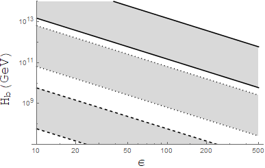
Figure 1: Examples of the parameter regions of $H_{b}$, $\epsilon$ and $\kappa$ that lead to successful Baryogenesis. The shaded regions subtended by the solid, dotted and dashed black lines depict the $\kappa=1,3,$ and 5 results respectively. The upper bounds correspond to the lower expectation of hypermagnetic field helicity to baryon number conversion, and vice versa.

The parameters required for successful Baryogenesis can be tested against the energy density constraint given in Eq. (33). First consider the constraints on $\epsilon^{2}H_{b}$ from Eq. (41) for the case of gauge field production until the bounce point, $H_{c}=H_{b}$,

$$\frac{1.5\cdot 10^{15}~{}\textrm{GeV}}{C(\kappa)^{2/3}}~{}<\epsilon^{2}|H_{b}|<~{}\frac{10^{17}~{}\textrm{GeV}}{C(\kappa)^{2/3}}~{},$$ (42)

hence, considering the maximum value, Eq. (33) becomes,

$$C(\kappa)^{\frac{1}{6}}\gg 0.05~{},$$ (43)

which is easily satisfied for $\kappa>1$. Therefore, the energy density constraint does not constrain on the parameter space when considering hypermagnetic field helicity generation up to the bounce point, and subsequent successful generation of the observed baryon asymmetry. Figure 1, depicts the parameter regions of successful Baryogenesis for different values of $\kappa$. Once $\kappa>5$, it becomes difficult to reconcile the parameters of $H_{b}$ and $\epsilon$ with the requirements of a consistent Ekpyrotic background evolution.

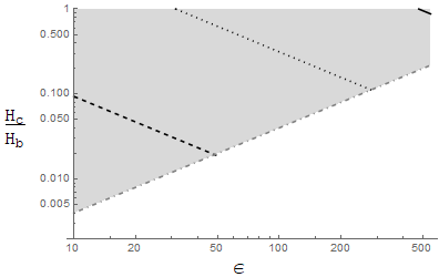
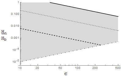
Figure 2: The allowed parameter space of $H_{c}$, $\epsilon$ and $\kappa$ that leads to successful Baryogenesis and satisfies the energy density constraint, where $T_{\rm rh}=10^{15}$ GeV and $H_{b}\simeq 10^{12}$ GeV has been selected. The left-hand and right-hand plots correspond to the lower and upper limits of Eq. (41), respectively. The dot-dashed grey line corresponds to the maximum energy density constraint given in Eq. (46), while the upper limit on $H_{c}$ is where $H_{c}=H_{b}$. The solid, dotted and dashed black lines depict the $\kappa=1,~{}3,$ and 5 cases respectively.

In the case of $|H_{c}|<|H_{b}|$, there is the following constraint due to successful Baryogenesis,

$$\frac{1}{\epsilon C(\kappa)^{1/3}}\sqrt{\frac{1.5\cdot 10^{15}~{}\textrm{GeV}}{|H_{b}|}}~{}<\frac{H_{c}}{H_{b}}<~{}\frac{1}{\epsilon C(\kappa)^{1/3}}\sqrt{\frac{10^{17}~{}\textrm{GeV}}{|H_{b}|}}~{},$$ (44)

which in combination with the energy density constraint of Eq. (33) becomes the $\kappa$-independent bound for the minimum and maximum of Eq. (40), respectively,

$$\frac{H_{c}}{H_{b}}\gg\frac{\epsilon T_{\rm rh}}{2.5\cdot 10^{20}~{}\textrm{GeV}}~{},~{}~{}\textrm{and}~{}~{}\frac{H_{c}}{H_{b}}\gg\frac{\epsilon T_{\rm rh}}{10^{23}~{}\textrm{GeV}}~{}.$$ (45)

In Figure 2, the parameter space for successful Baryogenesis and consistency with Eq. (45) is plotted, where the reheating temperature has been fixed to $T_{\rm rh}\sim 10^{15}$ GeV. In this case, the energy density constraints used are,

$$\frac{H_{c}}{H_{b}}\gtrsim 4\cdot 10^{-4}\epsilon~{},~{}~{}\textrm{and}~{}~{}\frac{H_{c}}{H_{b}}\gtrsim 10^{-6}\epsilon~{},$$ (46)

which leaves significant parameter space that can produce the observed baryon asymmetry.

These two scenarios generate large scale galactic magnetic fields. The evolution of the magnetic field and correlation length after the EWPT to the present day, is derived as,

$$B_{p}^{0}\simeq 2\cdot 10^{-18}~{}\textrm{G}~{}C(\kappa)^{1/3}\frac{H_{c}}{H_{b}}\left(\frac{\epsilon^{2}H_{b}}{10^{13}~{}\textrm{GeV}}\right)^{1/2}~{},$$ (47)

and

$$\lambda_{p}^{0}\simeq 6\cdot 10^{-5}~{}\textrm{pc}~{}C(\kappa)^{1/3}\frac{H_{c}}{H_{b}}\left(\frac{\epsilon^{2}H_{b}}{10^{13}~{}\textrm{GeV}}\right)^{1/2}~{}.$$ (48)

Applying the parameters required for successful Baryogenesis given in Eq. (41), the present day magnetic fields have magnitude and correlation length within the following ranges,

$$2.4\cdot 10^{-17}~{}\textrm{G}<B_{p}^{0}<2\cdot 10^{-16}~{}\textrm{G}~{},$$ (49)

and

$$7\cdot 10^{-4}~{}\textrm{pc}<\lambda_{p}^{0}<6\cdot 10^{-3}~{}\textrm{pc}~{},$$ (50)

with the upper and lower bound corresponding to the lower and upper limits of Eq. (40), respectively. These magnetic fields can lead to interesting observational signatures due to their helical nature [71]. The magnitude of these magnetic fields are below the current upper limits, but unfortunately are too small to explain the current Blazar results.

It should be noted that the present day magnetic fields that result from successful Baryogenesis in this Ekpyrotic mechanism are consistent with those for the Inflationary Baryogenesis scenario. Thus, observational results besides the magnetic fields and successful Baryogenesis are required to differentiate the two models. One avenue to achieve this is through gravitational waves, through measurements of the tensor-to-scalar ratio on CMB scales, and possible higher frequency chiral gravitational wave signatures produced by the gauge field production [72, 40]. As discussed in Section 2, the discovery of a tensor-to-scalar ratio in near future CMB experiments could place significant constraints on the Ekpyrotic scenario [54].

The enhanced production of gauge fields is known to be able to generate unique gravitational signatures [72, 40], which can provide an additional avenue for observational testing of these models. To see whether this leads to observational consequences in our model, we can compare the chiral gravitational waves sourced by the Hypermagnetic field generation by the fast rolling of $\varphi$ with those that are characteristic of Ekpyrotic Cosmologies, given in Eq. (15). The gravitational waves produced by gauge field production during an Ekpyrotic contraction phase have been calculated in Ref. [40], and found to exhibit a bluer spectrum than that already predicted in Ekpyrotic Cosmology. Namely,

$$\mathcal{P}^{s}_{T}\simeq 3.3\cdot 10^{-7}\frac{e^{4\pi\kappa}}{\kappa^{2}}\frac{k^{3}H_{b}}{M_{p}^{4}}~{},$$ (51)

for $\epsilon\gg 1$. Given that the two components of the gravitational wave spectrum are independent, $\mathcal{P}^{\textrm{Total}}_{T}(k)=\mathcal{P}^{v}_{T}(k)+\mathcal{P}^{s}_{T}(k)$, it is then possible to determine when the gravitational waves sourced from the gauge field production become important. The frequency range of observational interest, for which $\mathcal{P}^{s}_{T}(k)\geq\mathcal{P}^{v}_{T}(k)$ and successful Baryogenesis is achieved, is given by,

$$300\textrm{ MHz}\left(\frac{\kappa}{5}\right)^{8/3}e^{\frac{2\pi}{3}(5-\kappa)}>f>31\textrm{ kHz}\left(\frac{\epsilon}{25}\right)^{3}\left(\frac{\kappa}{5}\right)^{-2}e^{2\pi(5-\kappa)}~{},$$ (52)

where the upper bound for successful Baryogenesis in Eq. (42) has been utilised. For the lower bound of Eq. (42), the frequency range of interest is bounded by,

$$37\textrm{ MHz}\left(\frac{\kappa}{5}\right)^{8/3}e^{\frac{2\pi}{3}(5-\kappa)}>f>16\textrm{ MHz}\left(\frac{\epsilon}{25}\right)^{3}\left(\frac{\kappa}{5}\right)^{-2}e^{2\pi(5-\kappa)}~{},$$ (53)

where in both scenarios the upper frequency limit is derived from the cut-off $k\tau_{b}=2\kappa$, above which the effects of gauge field amplification are suppressed. For there to be significant observational consequences of the sourced gravitational waves, we require that $\kappa$ is large, $\epsilon$ is suppressed, and that the conversion of the Hypermagnetic field to baryon number at the EWPT is inefficient; as shown in Eq. (52). In this regime, the frequencies of interest tend to be higher, and require greater sensitivities, than those probed by existing experiments. Therefore, the gauge field production can generate features in the high frequency region of the gravitational wave spectrum, which if possible to probe in future could provide important information about the details of the Ekpyrotic mechanism. Although we have only mentioned the $H_{c}=H_{b}$ case, similar conclusions can likely be drawn for the $H_{c}<H_{b}$, dependent upon the details of the model.

Improved precision in the measurement of non-gaussianities and a detailed analysis of the predictions in this Ekpyrotic scenario, may play a key role in constraining the allowed parameter space for Baryogenesis. As discussed in Section 2, the non-gaussianities produced in Ekpyrotic Cosmology can be consistent with current observational measurements. However, in our scenario, additional non-gaussianities could be sourced by the Chern-Simons coupling between the Ekpyrotic scalar and Hypermagnetic field, possibly providing further avenues for testing the allowed parameter space. Given the dependence of this contribution on the details of the scalar sector, the period around the bounce point, and the possible utilisation of current mechanisms for reducing non-gaussianities in Ekpyrotic models, this will require a dedicated analysis that is to be completed in future work.

5 Conclusion

The Ekpyrotic cosmological model is able to provide solutions to the known cosmological problems as well as those associated with inflationary cosmology. We have proposed a mechanism for Baryogenesis that takes place during an Ekpyrotic contracting phase, prior to the bounce and onset of the standard radiation dominated epoch. If the evolution of the universe becomes dominated by a fast-rolling pseudoscalar with a negative exponential potential, a period of Ekpyrotic contraction can begin characterised by the equation of state $\omega\gg 1$. Coupling this pseudoscalar to the Standard Model Hypercharge gauge group, through a Chern-Simons term, leads to the generation of a non-zero Chern-Simons number density prior to the bounce point. The size of the produced Chern-Simons number density is found to explain the observed baryon asymmetry for a wide range of reasonable parameter choices.

The large range of allowed parameters bodes well for successful Baryogenesis with a more detailed analysis required to understand the full gauge field dynamics during the contracting phase, and possible back-reaction or suppression effects. In general, the non-gaussianities generated in Ekpyrotic models can be too large to be consistent with observation, unless a period of kination is induced by a secondary scalar field prior to the bounce. The presence of a second Ekpyrotic scalar motivated the consideration of the scenario of $|H_{c}|<|H_{b}|$ in our analysis, in such a case the Chern-Simons number generation will end when the background trajectory becomes dominated by this secondary scalar. This scenario gives a wide validity region in the parameter space for Baryogenesis, with constraints derived from the requirement of sub-dominance of the gauge field energy density.

The Hypercharge Chern-Simons coupling generates large scale magnetic fields, although the resultant magnitude and correlation length present today is unable to explain the Blazar results and Baryogenesis simultaneously. To do this would require an extra source of suppression of the conversion of hypercharge helicity to baryon asymmetry at the EWPT. The present day magnetic field predictions in our model are consistent with those of the analogous inflationary Baryogenesis scenario, further pointing to the duality of the slow and fast-roll parameters. This makes it difficult to distinguish between the two scenarios without additional observational predictions. Some avenues for differentiation are through the tensor-to-scalar ratio, high frequency gravitational waves and non-gaussianities; with improved precision of measurements and theoretical developments being required. These scenarios warrant further investigation due to their rich phenomenology and the wide ranging implications for our understanding of the evolution of the early universe.

References

- [1] N. Aghanim et al. [Planck Collaboration], arXiv:1807.06209 [astro-ph.CO].
- [2] A. D. Sakharov, Pisma Zh. Eksp. Teor. Fiz. 5, 32 (1967).
- [3] A. G. Cohen, D. B. Kaplan and A. E. Nelson, Ann. Rev. Nucl. Part. Sci. 43 (1993) 27 doi:10.1146/annurev.ns.43.120193.000331 [hep-ph/9302210].
- [4] A. H. Guth, Phys. Rev. D 23 (1981) 347.
- [5] A. D. Linde, Phys. Lett. B 108, 389 (1982);
- [6] A. Albrecht and P. J. Steinhardt, Phys. Rev. Lett. 48, 1220 (1982).
- [7] V. F. Mukhanov and G. V. Chibisov, JETP Lett. 33, 532 (1981) [Pisma Zh. Eksp. Teor. Fiz. 33, 549 (1981)].
- [8] J. Martin, C. Ringeval and V. Vennin, Phys. Dark Univ. 5-6 (2014) 75 doi:10.1016/j.dark.2014.01.003 [arXiv:1303.3787 [astro-ph.CO]].
- [9] S. H. -S. Alexander, M. E. Peskin and M. M. Sheikh-Jabbari, Phys. Rev. Lett. 96, 081301 (2006) [hep-th/0403069];
- [10] S. Alexander, A. Marciano and D. Spergel, JCAP 1304, 046 (2013) [arXiv:1107.0318 [hep-th]];
- [11] A. Maleknejad, M. Noorbala and M. M. Sheikh-Jabbari, arXiv:1208.2807 [hep-th];
- [12] A. Maleknejad, Phys. Rev. D 90 (2014) 2, 023542 [arXiv:1401.7628 [hep-th]].
- [13] N. D. Barrie and A. Kobakhidze, JHEP 1409 (2014) 163 [arXiv:1401.1256 [hep-ph]].
- [14] N. D. Barrie and A. Kobakhidze, Mod. Phys. Lett. A 32 (2017) no.14, 1750087 [arXiv:1503.02366 [hep-ph]].
- [15] M. M. Anber and E. Sabancilar, Phys. Rev. D 92 (2015) no.10, 101501 doi:10.1103/PhysRevD.92.101501 [arXiv:1507.00744 [hep-th]].
- [16] D. Jiménez, K. Kamada, K. Schmitz and X. J. Xu, JCAP 1712 (2017) 011 doi:10.1088/1475-7516/2017/12/011 [arXiv:1707.07943 [hep-ph]].
- [17] V. Domcke, B. von Harling, E. Morgante and K. Mukaida, JCAP 1910 (2019) no.10, 032 doi:10.1088/1475-7516/2019/10/032 [arXiv:1905.13318 [hep-ph]].
- [18] E. C. G. Stueckelberg, Helv. Phys. Acta 11, 225 (1938).
- [19] M. B. Green and J. H. Schwarz, Phys. Lett. 149B (1984) 117. doi:10.1016/0370-2693(84)91565-X
- [20] R. Brandenberger and P. Peter, Found. Phys. 47 (2017) no.6, 797 doi:10.1007/s10701-016-0057-0 [arXiv:1603.05834 [hep-th]].
- [21] M. Novello and S. E. P. Bergliaffa, Phys. Rept. 463 (2008) 127 doi:10.1016/j.physrep.2008.04.006 [arXiv:0802.1634 [astro-ph]].
- [22] J. L. Lehners, Phys. Rept. 465 (2008) 223 doi:10.1016/j.physrep.2008.06.001 [arXiv:0806.1245 [astro-ph]].
- [23] R. H. Brandenberger, Int. J. Mod. Phys. Conf. Ser. 01 (2011) 67 doi:10.1142/S2010194511000109 [arXiv:0902.4731 [hep-th]].
- [24] D. Battefeld and P. Peter, Phys. Rept. 571 (2015) 1 doi:10.1016/j.physrep.2014.12.004 [arXiv:1406.2790 [astro-ph.CO]].
- [25] A. Ijjas and P. J. Steinhardt, Class. Quant. Grav. 35 (2018) no.13, 135004 doi:10.1088/1361-6382/aac482 [arXiv:1803.01961 [astro-ph.CO]].
- [26] J. Khoury, B. A. Ovrut, P. J. Steinhardt and N. Turok, Phys. Rev. D 64 (2001) 123522 doi:10.1103/PhysRevD.64.123522 [hep-th/0103239].
- [27] D. H. Lyth, Phys. Lett. B 524 (2002) 1 doi:10.1016/S0370-2693(01)01374-0 [hep-ph/0106153].
- [28] J. Khoury, B. A. Ovrut, P. J. Steinhardt and N. Turok, Phys. Rev. D 66 (2002) 046005 doi:10.1103/PhysRevD.66.046005 [hep-th/0109050].
- [29] R. Brandenberger and F. Finelli, JHEP 0111 (2001) 056 doi:10.1088/1126-6708/2001/11/056 [hep-th/0109004].
- [30] D. H. Lyth, Phys. Lett. B 526 (2002) 173 doi:10.1016/S0370-2693(01)01438-1 [hep-ph/0110007].
- [31] P. J. Steinhardt and N. Turok, Phys. Rev. D 65 (2002) 126003 doi:10.1103/PhysRevD.65.126003 [hep-th/0111098].
- [32] J. L. Lehners, P. McFadden, N. Turok and P. J. Steinhardt, Phys. Rev. D 76 (2007) 103501 doi:10.1103/PhysRevD.76.103501 [hep-th/0702153 [HEP-TH]].
- [33] E. I. Buchbinder, J. Khoury and B. A. Ovrut, Phys. Rev. D 76 (2007) 123503 doi:10.1103/PhysRevD.76.123503 [hep-th/0702154].
- [34] E. I. Buchbinder, J. Khoury and B. A. Ovrut, JHEP 0711 (2007) 076 doi:10.1088/1126-6708/2007/11/076 [arXiv:0706.3903 [hep-th]].
- [35] Y. F. Cai, D. A. Easson and R. Brandenberger, JCAP 1208 (2012) 020 doi:10.1088/1475-7516/2012/08/020 [arXiv:1206.2382 [hep-th]].
- [36] A. Ijjas and P. J. Steinhardt, arXiv:1904.08022 [gr-qc].
- [37] J. M. Salim, N. Souza, S. E. Perez Bergliaffa and T. Prokopec, JCAP 0704 (2007) 011 doi:10.1088/1475-7516/2007/04/011 [astro-ph/0612281].
- [38] C. Li, R. H. Brandenberger and Y. K. E. Cheung, Phys. Rev. D 90 (2014) no.12, 123535 doi:10.1103/PhysRevD.90.123535 [arXiv:1403.5625 [gr-qc]].
- [39] Y. K. E. Cheung, J. U. Kang and C. Li, JCAP 1411 (2014) 001 doi:10.1088/1475-7516/2014/11/001 [arXiv:1408.4387 [astro-ph.CO]].
- [40] I. Ben-Dayan, JCAP 1609 (2016) 017 doi:10.1088/1475-7516/2016/09/017 [arXiv:1604.07899 [astro-ph.CO]].
- [41] A. Ito and J. Soda, Phys. Lett. B 771 (2017) 415 doi:10.1016/j.physletb.2017.05.017 [arXiv:1607.07062 [hep-th]].
- [42] R. Koley and S. Samtani, JCAP 1704 (2017) 030 doi:10.1088/1475-7516/2017/04/030 [arXiv:1612.08556 [gr-qc]].
- [43] J. Khoury, P. J. Steinhardt and N. Turok, Phys. Rev. Lett. 92 (2004) 031302 doi:10.1103/PhysRevLett.92.031302 [hep-th/0307132].
- [44] A. Ijjas and P. J. Steinhardt, Class. Quant. Grav. 33 (2016) no.4, 044001 doi:10.1088/0264-9381/33/4/044001 [arXiv:1512.09010 [astro-ph.CO]].
- [45] A. M. Levy, A. Ijjas and P. J. Steinhardt, Phys. Rev. D 92 (2015) no.6, 063524 doi:10.1103/PhysRevD.92.063524 [arXiv:1506.01011 [astro-ph.CO]].
- [46] R. Kallosh, J. U. Kang, A. D. Linde and V. Mukhanov, JCAP 0804 (2008) 018 doi:10.1088/1475-7516/2008/04/018 [arXiv:0712.2040 [hep-th]].
- [47] Y. Akrami et al. [Planck Collaboration], arXiv:1905.05697 [astro-ph.CO].
- [48] E. I. Buchbinder, J. Khoury and B. A. Ovrut, Phys. Rev. Lett. 100 (2008) 171302 doi:10.1103/PhysRevLett.100.171302 [arXiv:0710.5172 [hep-th]].
- [49] J. L. Lehners and P. J. Steinhardt, Phys. Rev. D 78 (2008) 023506 Erratum: [Phys. Rev. D 79 (2009) 129902] doi:10.1103/PhysRevD.78.023506, 10.1103/PhysRevD.79.129902 [arXiv:0804.1293 [hep-th]].
- [50] J. L. Lehners, Adv. Astron. 2010 (2010) 903907 doi:10.1155/2010/903907 [arXiv:1001.3125 [hep-th]].
- [51] A. Fertig, J. L. Lehners and E. Mallwitz, Phys. Rev. D 89 (2014) no.10, 103537 doi:10.1103/PhysRevD.89.103537 [arXiv:1310.8133 [hep-th]].
- [52] A. Ijjas, J. L. Lehners and P. J. Steinhardt, Phys. Rev. D 89 (2014) no.12, 123520 doi:10.1103/PhysRevD.89.123520 [arXiv:1404.1265 [astro-ph.CO]].
- [53] L. A. Boyle, P. J. Steinhardt and N. Turok, Phys. Rev. D 69 (2004), 127302 doi:10.1103/PhysRevD.69.127302 [arXiv:hep-th/0307170 [hep-th]].
- [54] M. Hazumi et al., J. Low. Temp. Phys. 194 (2019) no.5-6, 443-452 doi:10.1007/s10909-019-02150-5
- [55] V. A. Kuzmin, V. A. Rubakov and M. E. Shaposhnikov, Phys. Lett. 155B (1985) 36. doi:10.1016/0370-2693(85)91028-7
- [56] M. S. Turner and L. M. Widrow, Phys. Rev. D 37 (1988) 2743. doi:10.1103/PhysRevD.37.2743
- [57] W. D. Garretson, G. B. Field and S. M. Carroll, Phys. Rev. D 46 (1992) 5346 doi:10.1103/PhysRevD.46.5346 [hep-ph/9209238].
- [58] M. Joyce and M. E. Shaposhnikov, Phys. Rev. Lett. 79 (1997) 1193 doi:10.1103/PhysRevLett.79.1193 [astro-ph/9703005].
- [59] M. Giovannini and M. E. Shaposhnikov, Phys. Rev. D 57 (1998) 2186 doi:10.1103/PhysRevD.57.2186 [hep-ph/9710234].
- [60] M. Giovannini, Phys. Rev. D 61 (2000) 063502 doi:10.1103/PhysRevD.61.063502 [hep-ph/9906241].
- [61] M. M. Anber and L. Sorbo, JCAP 0610 (2006) 018 doi:10.1088/1475-7516/2006/10/018 [astro-ph/0606534].
- [62] K. Bamba, Phys. Rev. D 74 (2006) 123504 doi:10.1103/PhysRevD.74.123504 [hep-ph/0611152].
- [63] J. Martin and J. Yokoyama, JCAP 0801 (2008) 025 doi:10.1088/1475-7516/2008/01/025 [arXiv:0711.4307 [astro-ph]].
- [64] V. Demozzi, V. Mukhanov and H. Rubinstein, JCAP 0908 (2009) 025 doi:10.1088/1475-7516/2009/08/025 [arXiv:0907.1030 [astro-ph.CO]].
- [65] R. Durrer, L. Hollenstein and R. K. Jain, JCAP 1103 (2011) 037 doi:10.1088/1475-7516/2011/03/037 [arXiv:1005.5322 [astro-ph.CO]].
- [66] C. Caprini and L. Sorbo, JCAP 1410 (2014) 056 doi:10.1088/1475-7516/2014/10/056 [arXiv:1407.2809 [astro-ph.CO]].
- [67] P. Adshead, J. T. Giblin, T. R. Scully and E. I. Sfakianakis, JCAP 1610 (2016) 039 doi:10.1088/1475-7516/2016/10/039 [arXiv:1606.08474 [astro-ph.CO]].
- [68] K. Kamada and A. J. Long, Phys. Rev. D 94 (2016) no.6, 063501 doi:10.1103/PhysRevD.94.063501 [arXiv:1606.08891 [astro-ph.CO]].
- [69] K. Kamada and A. J. Long, Phys. Rev. D 94 (2016) no.12, 123509 doi:10.1103/PhysRevD.94.123509 [arXiv:1610.03074 [hep-ph]].
- [70] C. Caprini, M. C. Guzzetti and L. Sorbo, Class. Quant. Grav. 35 (2018) no.12, 124003 doi:10.1088/1361-6382/aac143 [arXiv:1707.09750 [astro-ph.CO]].
- [71] H. Tashiro, W. Chen, F. Ferrer and T. Vachaspati, Mon. Not. Roy. Astron. Soc. 445 (2014) no.1, L41 doi:10.1093/mnrasl/slu134 [arXiv:1310.4826 [astro-ph.CO]].
- [72] J. L. Cook and L. Sorbo, Phys. Rev. D 85 (2012), 023534 doi:10.1103/PhysRevD.85.023534 [arXiv:1109.0022 [astro-ph.CO]].