Global Chemistry and Thermal Structure Models for the Hot Jupiter WASP-43b and Predictions for JWST
Abstract
The James Webb Space Telescope (JWST) is expected to revolutionize the field of exoplanets. The broad wavelength coverage and the high sensitivity of its instruments will allow characterization of exoplanetary atmospheres with unprecedented precision. Following the Call for the Cycle 1 Early Release Science Program, the Transiting Exoplanet Community was awarded time to observe several targets, including WASP-43b. The atmosphere of this hot Jupiter has been intensively observed but still harbors some mysteries, especially concerning the day-night temperature gradient, the efficiency of the atmospheric circulation, and the presence of nightside clouds. We will constrain these properties by observing a full orbit of the planet and extracting its spectroscopic phase curve in the 5–12 m range with JWST/MIRI. To prepare for these observations, we performed an extensive modeling work with various codes: radiative transfer, chemical kinetics, cloud microphysics, global circulation models, JWST simulators, and spectral retrieval. Our JWST simulations show that we should achieve a precision of 210 ppm per 0.1 m spectral bin on average, which will allow us to measure the variations of the spectrum in longitude and measure the night-side emission spectrum for the first time. If the atmosphere of WASP-43b is clear, our observations will permit us to determine if its atmosphere has an equilibrium or disequilibrium chemical composition, providing eventually the first conclusive evidence of chemical quenching in a hot Jupiter atmosphere. If the atmosphere is cloudy, a careful retrieval analysis will allow us to identify the cloud composition.
1 Introduction
Giant planets that orbit very close to their host stars — so-called “hot Jupiters” — are expected to be tidally locked, with one hemisphere constantly facing the star, and one hemisphere in perpetual darkness. The uneven stellar irradiation incident on such planets leads to strong and unusual radiative forcing, resulting in large temperature gradients and complicated atmospheric dynamics. The atmospheric composition and cloud structure on these planets can, in turn, vary in three dimensions as the temperatures change across the globe, and as winds transport constituents from place to place. Strong couplings and feedbacks between atmospheric chemistry, cloud formation, radiative transfer, energy transport, and atmospheric dynamics exist to further influence atmospheric properties. The inherently non-uniform nature of these atmospheres complicates derivations of atmospheric properties from transit, eclipse, and phase curve observations. Three-dimensional models that can track the relevant physics and chemistry on all scales — both large and small distance scales, and large and small time scales — are needed to accurately interpret hot Jupiter spectra.
Discovered in 2011 by Hellier et al. (2011), the hot Jupiter WASP-43b orbits a relatively cool K7V star (4 520 120 K, Gillon et al. 2012111Note that the stellar effective temperature has been re-estimated to 216 K by Sousa et al. (2018) after our models have been run.). It has the smallest semi-major axis of all confirmed hot Jupiters and one of the shortest orbital periods (0.01526 AU and 19.5 h respectively, Gillon et al. 2012). In addition to its exceptionally short orbit, WASP-43b is very good candidate for in-depth atmospheric characterization through transit thanks to its large planet-star radius ratio and the brightness of its host star, leading to a very good signal-to-noise ratio. The planet is also a good candidate for eclipse and phase curve observations thanks to the important flux ratio between the emission of the star and the exoplanet.
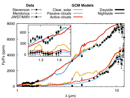
To date, many observations of the planet’s atmosphere have been conducted from the ground (Gillon et al., 2012; Wang et al., 2013; Chen et al., 2014; Murgas et al., 2014; Zhou et al., 2014; Jiang et al., 2016; Hoyer et al., 2016) and from space (Blecic et al., 2014; Kreidberg et al., 2014; Stevenson et al., 2014, 2017; Ricci et al., 2015). Most notably, orbital phase curves have been observed with both the Hubble Space Telescope (HST) from to (Stevenson et al., 2014) and with the Spitzer Space Telescope at and (Stevenson et al., 2016). Whereas these observations were able to constrain the dayside temperature structure and water abundances, they revealed the presence of a surprisingly dark nightside. Indeed neither Hubble nor Spitzer were able to measure the nightside flux from the planet. Poor energy redistribution (Komacek & Showman, 2016), high metallicity (Kataria et al., 2015), disequilibrium chemistry (Mendonça et al., 2018b) or the presence of clouds (Kataria et al., 2015) were proposed to explain this mystery.
The James Webb Space Telescope (JWST) is expected to transform our understanding of the complexity of hot Jupiters atmospheres thanks to the numerous observations of transiting hot Jupiters it will perform. Rapidly after the launch and commissioning of the JWST, exoplanet spectra will be obtained in the framework of the Transiting Exoplanet Community Early Release Science (ERS) Program (Bean et al., 2018). Three hot Jupiters will be observed using the different instruments of the JWST and the data will be available immediately to the community. Among these, WASP-43b is the nominal target that will be observed during the sub-program “MIRI Phase Curve”. A full orbit phase curve, covering two secondary eclipses and one transit, will be acquired with MIRI (Rieke et al., 2015). We will observe WASP-43b with MIRI during the Cycle 1 ERS Program developed by the Transiting Exoplanet Community (PIs: N. Batalha, J. Bean, K. Stevenson; Stevenson et al., 2016; Bean et al., 2018). The MIRI phase curve is our best opportunity to probe the cooler nightside of the planet, determine the presence and composition of clouds, detect the signatures of disequilibrium chemistry and more precisely measure the atmospheric metallicity. The MIRI phase curve will be complemented by a NIRSpec phase curve (GTO program 1224, Pi: S. Birkmann). The later will provide a robust estimate of the water abundances on the dayside of the planet but will probably not be able to obtain decisive information about the nightside. MIRI will observe the planet at longer wavelengths where the thermal emission is more easily detectable and provide the first spectrum of the nightisde of a hot Jupiter. Correctly interpreting the incoming data will be, however, challenging. As shown by Feng et al. (2016), many pitfalls including biased detection of molecules can be expected if a thorough modelling framework has not been developed.
To prepare these observations, intensive work has been carried out by members of the Transiting Exoplanet ERS Team to model WASP-43b’s atmosphere. In Section 2, we present the methodology of this paper and explain how our different models interact with each other. In Section 3, we present the models, parameters, and assumptions that have been used in this study. In Section 4, we show the results we obtained with these models concerning the thermal structure, the chemical composition, and the cloud coverage. In Section 5, we simulate the data that we expect to obtain with JWST, and we perform a retrieval analysis in Section 6. Finally, the conclusions are presented in Section 7.
2 Strategy
No single model is capable of simulating all the processes in an exoplanet atmosphere at once. The atmosphere must be modeled over many orders of magnitude in length scale (ranging from microphysical cloud formation to planet-wide atmospheric circulation). Planets are inherently 3D, and 1D models do not capture the expected variation in temperature, chemistry, or cloud coverage with location. It is not computationally feasible to include all the relevant effects in a single model. To simulate spectra for WASP-43b that are as complete as possible, we run a suite of models with a wide range of simplifying assumptions (1D, 2D, and 3D; equilibrium and disequilibrium chemistry). Each model is used as input for others. A major goal of this work is also to determine which modeling components are really necessary, or on the contrary can be substitute (i.e. we will see in Sect.4.1 that a 2D radiative/convective model can be a good alternative to a Global Circulation Model to calculate the thermal structure of a planet). Our methodology is represented on Figure 1 and detailed hereafter.
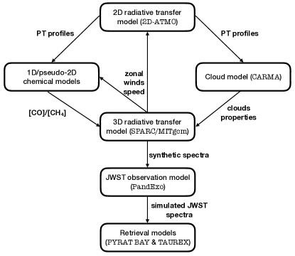
- Radiative/convective equilibrium models (2D) and general circulation models (GCM, 3D) have been used to compute the physical structure of the atmosphere. These two models indicate the temperatures all around the globe and thus quantify the day/night thermal gradient. The 3D model gives the zonal winds speeds that have been averaged (4.6 km.s-1) and used by the 2D radiative/convective model as well as the pseudo-2D chemical model. Assuming a thermochemical equilibrium composition, both give very similar results (see Sect. 4.1). Thus the 2D thermal profiles have been used as inputs in the chemical kinetics models. To simulate a disequilibrium composition, the 3D model uses the outputs of the chemical kinetics models, e.g. the average [CO]/[CH4] ratio. For the cloudy modeling, the 3D model uses the findings of the microphysical cloud model, e.g. the nature of the clouds. Finally, the main outputs of the 3D model are the planetary spectra that have been binned by our JWST simulator and then used to perform the retrieval.
- Chemical kinetics models (1D and pseudo-2D) have been used to determine the chemical composition of the atmosphere, taking into account a detailed chemistry and out-of-equilibrium processes (photochemistry and mixing). These models predict whether the atmosphere is in thermochemical equilibrium. The comparison between the 1D and the pseudo-2D model enables an assessment of the influence of horizontal circulation on the chemical composition and whether we should expect a gradient of composition between the day and night sides. The inputs necessary for these models are the 2D thermal profiles calculated with the 2D radiative/convective model, as well as the zonal wind speed, whose average value comes from the “equilibrium” GCM model. In return, the GCM model uses the findings of the chemical kinetics model to set up the [CO]/[CH4] in the “quenched” chemistry 3D model.
- Properties of clouds in the atmosphere of WASP-43b have been calculated using a cloud microphysical model. The findings of this model are informative about the possible location of clouds in the atmosphere, as well as the particle size and the nature of clouds. Determining the cloud coverage of the atmosphere is crucial as clouds tend to block the emitted flux of the planet and thus make harder the analyse of observational data. The cloud model uses as inputs the 2D thermal profiles. The outputs of this model (the nature of clouds and the particle size) was used in the cloudy 3D model.
- Another series of models have been used to simulate the observations and their spectral analysis. The synthetic emission spectra (dayside and nightside) predicted by the GCM have been put through an instrument simulator to reproduce the instrumental noise and resolution of the JWST instrument MIRI. The outputs of this simulator are then directly used by retrieval models.
- Finally, we used retrieval models to determine what information we will be able to extract from the new observations. This last step also permits to raise the difficulties that we will have to face and thus highlight which efforts/precautions will be required for the analyse of WASP-43b data. These models use the outputs of the JWST simulator.
All the models used at each step are presented and detailed in the following subsections. It is important to note that the findings of each model are dependent on the intrinsic assumptions and design of each model. For instance, the retrieval models can only retrieve information that these models contain. It does, however, not mean that the presence of other molecules is thereby excluded. The physical properties of WASP-43b and its host star used in all the models are gathered in Table 1.
| Parameter | Valuea |
|---|---|
| Stellar Mass | 0.717 ( 0.025) M☉ |
| Stellar Radius | 0.667 ( 0.01) R☉ |
| Effective Temperature | 4 520 ( 120 ) K |
| Planetary Mass | 2.034 ( 0.052) MJ |
| Planetary Radius | 1.036 ( 0.019) RJ |
| Semi-major Axis | 0.01526 AU |
Reference. a Gillon et al. (2012).
3 Description of the models
3.1 Radiative Transfer Model
ATMO is a 1D/2D atmospheric model that solves the radiative/convective equilibrium with and without irradiation from an host star. It has been used for the study of brown dwarfs and directly imaged exoplanets (Tremblin et al., 2015, 2016, 2017b; Leggett et al., 2016, 2017), and also for the study of irradiated exoplanets (Drummond et al., 2016; Wakeford et al., 2017; Evans et al., 2017). The gas opacity is computed by using the correlated-k method (Lacis & Oinas, 1991; Amundsen et al., 2014, 2017) including the following species in this study: H2-H2, H2-He, H2O, CO, CO2, CH4, NH3, K, Na, Li, Rb, Cs from the high temperature ExoMol (Tennyson & Yurchenko, 2012) and HITEMP (Rothman et al., 2010) line list databases. We use 32 frequency bins between 0.2 and 320 m with 15 k-coefficients per bin. The chemistry is solved at equilibrium or out-of-equilibrium by a consistent coupling with the chemical kinetic network of Venot et al. (2012). 1D-ATMO has been recently benchmarked against Exo-REM and petitCODE (Baudino et al., 2017).
In this study, we have used 2D-ATMO, an extension of 1D-ATMO (Tremblin et al., 2017a) that takes into account the circulation induced by the irradiation from the host star at the equator of the planet. We have taken a Kurucz spectrum (Castelli & Kurucz, 2004) for WASP-43 with a radius of 0.667 R☉, an effective temperature of 4500 K, and a gravity of log() = . The magnitude of the zonal wind is imposed at the substellar point at 4 km/s and is computed accordingly to the momentum conservation law in the rest of the equatorial plane. The vertical mass flux is assumed to be proportional to the meridional mass flux with a proportionality constant ; the wind is therefore purely longitudinal and meridional if or purely longitudinal and vertical for . As in Tremblin et al. (2017a), a relatively low value of drives the vertical advection of entropy/potential temperature in the deep atmosphere that can produce a hot interior, which can explain the inflated radii of hot Jupiters. A high value of will produce a "cold" deep interior as in the standard 1D models. In this study, we have used two values of , 10 and 104 to explore these two limits. The simulation with =104 should be more representative of WASP-43b since the planet is not highly inflated.
3.2 3-D Circulation Models
SPARC/MITgcm couples a state-of-the art non-grey, radiative transfer code with the MITgcm (Showman et al., 2009). The MITgcm solves the primitive equations on a cube-sphere grid (Adcroft et al., 2004). It is coupled to the non-grey radiative transfer scheme based on the plane-parallel radiative transfer code of Marley & McKay (1999). The stellar irradiation incident on WASP-43b is computed with a Phoenix model (Hauschildt et al., 1999). The opacities we use are described in Freedman et al. (2008), including more recent updates (Freedman et al., 2014), and the molecular abundances are calculated assuming local chemical equilibrium (Visscher et al., 2010). In the 3D simulation, the radiative transfer calculations are performed on 11 frequency bins ranging from 0.26 to 300 m, with 8 k-coefficients per bin statistically representing the complex line-by-line opacities. For calculating the spectra the final SPARC/MITgcm thermal structure is post-processed with the same radiative transfer code but using a higher spectral resolution of 196 spectral bins (Fortney et al., 2006). We initialize the code with the analytical planet-averaged pressure-temperature profile of Parmentier et al. (2015a), run the simulation for 300 days and average all physical quantities over the last 100 days of simulation.
Our baseline model is a solar-composition, cloudless model. We also performed simulations including the presence of radiatively active clouds and radiatively passive clouds following the method outlined in Parmentier et al. (2016). Finally, models assuming a constant [CO]/[CH4] ratio were also performed, following the method outlined in Steinrueck et al. (2018). These latter models simulate out-of-equilibrium transport-induced quenching of CO and CH4.
3.3 Chemical Kinetics Models
To address the variations of atmospheric chemical composition with altitude and longitude, we used both 1D and 2D chemical kinetics models. We describe here these two codes.
3.3.1 1D chemical kinetics model
The thermo-photochemical model developed by Venot et al. (2012) is a full 1D time-dependent model. This model takes into account a detailed chemical kinetics and the out-of-equilibrium processes of photodissociation and vertical mixing (eddy and molecular diffusion). The atmospheric composition is computed for a fixed thermal profile divided in discrete layers, solving the continuity equations for each species until steady-state is reached. No flux of species is imposed at the boundaries of the atmosphere. In this study, we used the C0-C2 chemical kinetic network, which contains 2000 reactions describing the kinetics of 105 species made of H, C, O, and N, with up to two carbon atoms. This chemical scheme has been developed in close collaboration with specialists in combustion and validated experimentally on wide ranges of pressure and temperature as a whole (i.e. not only each reaction individually) leading to a high reliability. Since we consider both direction (forward and reverse) for each reaction, in absence of out-of-equilibrium processes, thermochemical equilibrium is achieved kinetically. To these 2000 reactions, 55 photodissociations have been added to model the interaction of incoming UV flux with molecules. These reactions are of course not reversed due to the disequilibrium irreversible nature of this process. A complete description of the model and the chemical scheme can be found in Venot et al. (2012). The kinetic model has been applied to several exoplanetary atmospheres (Venot et al., 2012, 2013, 2014, 2016; Agúndez et al., 2014b; Tsiaras et al., 2016; Rocchetto et al., 2016) and the deep atmosphere of Saturn (Mousis et al., 2014), Uranus (Cavalié et al., 2014, 2017), and Neptune (Cavalié et al., 2017).
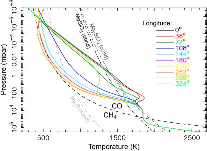
Using this 1D chemical kinetics model, we determined the chemical composition of the atmosphere of WASP-43b at different longitudes around the equator. The vertical temperature structure as a function of longitude is taken from the 2D radiative-transfer models (Section 3.1) utilizing =104 since the planet is not highly inflated. We extended these profiles to higher altitudes using extrapolation, and the resulting profiles are shown in Fig. 3. Each longitude has been computed until steady-state is reached, independently from each other, starting from the thermochemical equilibrium corresponding to the thermal structure. The stellar zenith angle varied with longitude. Given the characteristics of the host star, we estimated the incident stellar spectrum using the same Kurucz (Castelli & Kurucz, 2004) stellar model than in 2D-ATMO for wavelengths 2200 Å, an IUE spectrum of GL 15B scaled by a factor of 10 for the 1250-2200 Å region, and the solar maximum spectrum of Woods & Rottman (2002) scaled by a factor of 1.36 (see Czesla et al., 2013) for wavelengths less than 1250 Å. Vertical transport operates through eddy and molecular diffusion, with an assumed eddy diffusion coefficient profile that varies as (cm2 s-1) = 10 throughout the bulk of the planet’s infrared photosphere, independent of longitude, except approaches a constant-with-altitude value of 1010 cm2 s-1 at high altitudes and at pressures greater than 300 bar (Figure 2). As a large uncertainty resides for this parameter, we chose to use an expression similar to the one adopted for HD 189733b based on GCM passive tracer transport (Agúndez et al., 2014a). This method gives values for the vertical mixing much lower (up to 1000 times) than the classical root-mean-square (rms) method (Agúndez et al., 2014a; Charnay et al., 2015). A correct estimation of this parameter is crucial as it determines the quenching level and thus the molecular abundances of some fundamental species (e.g. Miguel & Kaltenegger, 2014; Venot et al., 2014; Tsai et al., 2017). Solar proportions of elemental abundances are assumed (Lodders, 2010) with a depletion of 20% in oxygen due to the sequestration in silicates and metals (Lodders, 2004). No TiO/VO has been included.
3.3.2 2D chemical kinetics model
Based on the procedure of Agúndez et al. (2014a), for this study we developed a “pseudo-2D” chemical model to track how the atmospheric composition of WASP-43b would vary as a function of altitude and longitude, and hence orbital phase. We assume that longitudes are not isolated from each other (as in the 1D chemical model) rather connected through a strong zonal jet. Tidal interactions between host stars and gas giant planets are expected to circularize the planet orbit and synchronize the rotation period of the planet (Lubow et al., 1997; Guillot & Showman, 2002). The timescale for this to happen is much shorter than the stellar lifetime when the planet orbit is shorter than 10 days such as for WASP-43b (see Fig.1 of Parmentier et al., 2015b). With one hemisphere constantly facing the star, the unequal stellar forcing produces strong zonal winds that transport heat and chemical constituents across the dayside and into the nightside of the planet, and back again (e.g., Showman et al. 2010; see also the GCM results in Section 4.4). This zonal transport provides “diurnal” variation in temperatures and stellar irradiation from the point of view of a parcel of gas being transported by the winds. If chemical equilibrium were to prevail in WASP-43b’s atmosphere, the composition would be very different on the colder nightside in comparison to the hotter dayside. However, if the horizontal transport by the zonal winds is faster than the rate at which chemical constituents can be chemically converted to other constituents, then the composition can be “quenched” and remain more uniform with longitude (e.g., Cooper & Showman 2006; Agúndez et al. 2014a). Our pseudo-2D model tracks the time variation in atmospheric composition as a function of altitude and longitude as an atmospheric column at low latitudes experiences this pseudo-rotation.
Our pseudo-2D thermo/photochemical kinetics model uses the Caltech/JPL KINETICS code (Allen et al., 1981) as its base, modified for exoplanets as described in Moses et al. (2011, 2013a, 2013b, 2016), along with the pseudo-2D procedure described in Agúndez et al. (2014a). The model contains 1870 reactions (i.e., 900 forward and reverse pairs) involving 130 different carbon-, oxygen-, nitrogen-, and hydrogen-bearing species whose rate coefficients have been reversed using the thermodynamic principle of reversibility (see Visscher & Moses, 2011). Photolysis reactions are included and have not been reversed. The reaction list is taken from the GJ 436b model of Moses et al. (2013b), and includes H, C, O, N species. Molecules with up to six carbon atoms are included, but the possible chemical production and loss pathways in the model become less complete the heavier the molecule. Note that the chemical reactions list used in the pseudo-2D model slightly differs from that of the 1D chemical model. The departures between these two chemical schemes and their implications on the calculated abundances have already been addressed in several studies (Venot et al., 2012; Moses, 2014; Wang et al., 2016): depending on the scheme used, the quench level and resulting quenched abundances of some species are somewhat different. For instance, for HD 209458b-like planets, the quenched mixing ratio of CH4 will be twice as large with Moses et al. (2013b)’s scheme as with Venot et al. (2012)’s. However, the goal of our study here is to qualitatively compare the expected longitudinal variation obtained with the 1D and pseudo-2D chemical models in order to evaluate the effect of horizontal circulation on the global composition and transport/eclipse observations, and to determine a rough CO/CH4 ratio to be used in the 3D GCM. Comparing results between the 1D and pseudo-2D chemical models described here adequately addresses these goals. Other model inputs, including the boundary conditions and vertical diffusion coefficients adopted in the model, are identical to 1D chemical kinetics model described above.

Following Agúndez et al. (2014a), our pseudo-2D approach is to solve the 1D continuity equations for a vertical column of gas at the equator as it rotates around the planet with a constant average low-latitude jet speed of 4.6 km s-1 (based on the GCM results described in Section 4.4). As it has been discussed in Agúndez et al. (2012, 2014a), assuming a uniform zonal wind is a good approximation for equatorial region, dominated by a superrotating jet (Kataria et al., 2015). This approximation might be inadequate for latitudes towards the poles, when the circulation regime is more complex. Both the stellar zenith angle and atmospheric temperatures vary with time as the gas column rotates through different longitudes, both affecting the atmospheric chemistry. The vertical temperature structure as a function of longitude is fixed and is the same as that used in the 1D chemical kinetics model (Fig. 3). The eddy diffusion profile ( coefficient profile) is also similar to that of the 1D chemical kinetics model (Fig. 2). The planet is divided into different longitude regions, and the system of differential equations making up the continuity equations is integrated over the amount of time it would take a parcel of gas at the equator to be transported from one discretized longitude to the next discretized longitude. At that point, the mixing ratios as a function of pressure at the end of the first longitude calculation are fed in as initial conditions to the next longitude calculation, with its new thermal structure and incident UV flux that depends on the new zenith angle. The temporal evolution of this equatorial column of gas is followed for 20 full planetary “rotations” to provide sufficient time for the species produced photochemically at high altitudes to be transported down through the atmosphere to deeper regions where thermochemical equilibrium dominates. At that point, the “daily” longitude variations were consistent from one pseudo-rotation to the next. Agúndez et al. (2012) discuss the various advantages of beginning the pseudo-2D calculations at the hottest dayside conditions. Based on their discussion, we use the results of a 1D thermo/photochemical kinetics model for conditions at the substellar point (longitude 0˚) that has been run long enough to reach steady state as our initial conditions for the pseudo-2D model.
3.4 Cloud Microphysics Model
We use the Community Aerosol and Radiation Model for Atmospheres (CARMA; Turco et al., 1979; Toon et al., 1988; Jacobson & Turco, 1994; Ackerman et al., 1995) to investigate the vertical and longitudinal distribution of clouds in the atmosphere of WASP-43b. While we do not include the resulting distributions in our GCM simulations, we will be able to extract insights into the effect of longitudinal temperature variations on cloud distributions. CARMA is a 1D cloud microphysics model that generates binned size distributions of aerosol particles as a function of altitude (pressure) in an atmospheric column by explicitly computing and balancing the rates of cloud particle nucleation, growth by condensation and coagulation, loss by evaporation, and transport by sedimentation, advection, and diffusion. This sets CARMA apart from simpler cloud condensation models (e.g. Fegley & Lodders, 1994; Ackerman & Marley, 2001), which assume cloud formation as soon as the condensate vapor saturates. The equations CARMA solves to evaluate the rates of these processes are presented in the Appendix of Gao et al. (2018). CARMA has been applied to aerosol processes across the solar system (Colaprete et al., 1999; Barth & Toon, 2003; Bardeen et al., 2008; Gao et al., 2014, 2017), and has recently been used to simulate Al2O3, TiO2, MgSiO3 (enstatite), KCl, and ZnS clouds on exoplanets and brown dwarfs (Gao et al., 2018; Powell et al., 2018; Gao & Benneke, 2018).
For this work, we include additional condensates that have been hypothesized to dominate the condensate mass in exoplanet atmospheres, including Mg2SiO4 (forsterite), Fe, Cr, MnS, and Na2S (Lodders, 1999; Visscher et al., 2006; Helling et al., 2008; Visscher et al., 2010). Additional condensates are possible, as shown in grain chemistry models (e.g. Helling & Woitke, 2006), but we do not treat them here, as it would be computationally prohibitive. In addition, to reduce the number of different condensates we assume that forsterite is the primary silicate condensate rather than modeling both forsterite and enstatite clouds. This is based on the argument that a rising parcel of vapor would see forsterite condense first due to it having higher condensation temperatures than enstatite; this depletes Mg and SiO, such that the enstatite cloud that forms above the forsterite cloud should have significantly lower mass. We discuss the implications of this assumption in the Sect. 4.3. As with the treatment of enstatite in Powell et al. (2018), we assume forsterite and Fe clouds form by heterogeneously nucleating on TiO2 seeds, as direct nucleation of these two species from vapor is slow (Helling & Woitke, 2006; Gao et al., 2018). All other condensates are assumed to nucleate homogeneously.The saturation vapor pressures of Cr, MnS, and Na2S are taken from Morley et al. (2012). The surface energy of Cr is calculated from the Eötvös rule, while for MnS and Na2S we assume the same surface energy as that of KCl. The size distribution for each condensate species is calculated separately, and so a distinct size distribution exists for each species.
As in the 1D and pseudo-2D chemical kinetics models, we use fixed pressure-temperature profiles described in Section 3.1 for our background atmosphere. All planetary parameters used are the same as those of the other models presented here to ensure consistency. In the cloud microphysics model, we use a very similar profile as the one used in the chemical kinetics models (Figure 2), except we set a minimum of 107 cm2 s-1. This change only affects pressures 1 bar, where the chemical kinetics model is 107 cm2 s-1. We also reduce the high at pressures 300 bar to our minimum value. This was necessary to reduce model run time and numerical instabilities. An atmospheric column is simulated at each longitude independently of each other, under the assumption that microphysical timescales are short compared to horizontal transport timescales, though this may not be the case for all pressure levels and particle sizes (Powell et al., 2018). For each column, we investigate distinct clouds composed of Al2O3, TiO2, Mg2SiO4, Fe, Cr, MnS, Na2S, ZnS, and KCl, though which clouds actually form depends on which species is supersaturated and their nucleation rates. We assume solar abundances for the limiting elements of these clouds, which are, in the same order, Al, TiO2, Mg, Fe, Cr, Mn, Na, Zn, and KCl.
Importantly, the vertical, longitudinal, and particle size distributions computed by this model are not used to generate synthetic observations, as will be presented later in this work. This is due to the uncertainties in the material properties of some of the condensates (e.g. surface energies of MnS and Na2S) and the way exoplanet clouds form, whether through homogeneous nucleation, heterogeneous nucleation on some foreign condensation nuclei, or grain chemistry (Helling & Woitke, 2006). Instead, results from CARMA will be helpful for informing general GCM and retrieval studies due to its ability to compute the relative abundances of different cloud species in the atmosphere of WASP-43b, thus indicating the species that affect the observations the most. Simplified cloud models can then be used to explore the parameter space around these results.
3.5 JWST Observation Model
WASP-43b is the primary target for the “MIRI Phase Curve” observation that will be carried out as part of the Transiting Exoplanet JWST Early Release Science Program. The goal is to observe a full orbit of WASP-43b including two eclipses and one transit in the wavelength range 5–12m at a resolution with MIRI LRS (Low Resolution Spectroscopy) in slitless mode (Kendrew et al., 2015). In that program, the planetary emission spectra as a function of longitude will be measured and relevant atmospheric properties retrieved. We simulate the expected outcomes of this observation using the PandExo222https://exoctk.stsci.edu/pandexo/ software program (Batalha et al., 2017). PandExo is a noise simulator specifically designed for transiting exoplanet observations with JWST and HST, and includes all observatory-supported time-series spectroscopy modes.
The input parameters for the star and planet are those indicated in Table 1. The stellar spectrum is obtained from the NextGen (Hauschildt et al., 1999) grid interpolated at the and log() of WASP-43 and is the same as used in the 3D SPARC/MITgcm. We consider a range of planetary emission spectra derived from the 3D SPARC/MITgcm model described in Section 3.2, with or without clouds, assuming thermochemical equilibrium or a quenched [CH4]/[CO] ratio. These simulations are performed with similar inputs as those used for the JWST ERS Program proposal (PIs: N. Batalha, J. Bean, K. Stevenson; Bean et al., 2018): the radiative transfer models, the star and planet parameters and input spectra, and the observation parameters are the same (here we simulate a broader range of planetary spectra).
The planetary spectra are calculated from the emission integrated over the visible hemisphere. For this work, we simulate spectra with a spacing of 20˚ in longitude and use them as inputs for PandExo. We consider that we observe each longitude during one eighteenth of the orbital period (1.08 hours) and we use a baseline of twice the eclipse duration because we will observe two eclipses (2.32 hours). In practice, the longitude 0˚ will be in-eclipse so we may have to split the orbit slightly differently, but for these simulations we treat this longitude as the other ones. The resolution and instrumental parameters are those of MIRI LRS. The wavelength range goes up to m but we consider only the 5–12m range because the efficiency of LRS decreases significantly beyond 12m. We use a saturation level of 80% of the full well. The details of the noise modelling can be found in Batalha et al. (2017).
3.6 Retrieval models
To retrieve the atmospheric properties of WASP-43b, we use two models: TauREx333https://github.com/ucl-exoplanets (Waldmann et al., 2015b, a; Rocchetto et al., 2016) and the Python Radiative Transfer in a Bayesian framework (Pyrat Bay444http://pcubillos.github.io/pyratbay, Cubillos et al. 2019, in prep., Blecic et al. 2019a,b, in prep.). Both, TauREx and Pyrat Bay are open-source retrieval frameworks that compute radiative-transfer spectra and fit planetary atmospheric models to a given set of observations. The atmospheric models consist of parameterized 1D profiles of the temperature and species abundances as a function of pressure, with atomic, molecular, collision-induced, Rayleigh, and cloud opacities. We decide to use two codes that don’t use the same retrieval methods in order to compare the results obtained and raise the eventual biases that could emerge. We present hereafter the two codes.
3.6.1 TauREx
The TauREx model can retrieve equilibrium chemistry using the ACE code (Agúndez et al., 2012) as well as perform so-called “free” retrievals where trace gas volume mixing ratios are left to vary as free parameters. For this study, all the retrieval models used the “free chemistry” method. The statistical sampling of the log-likelihood is performed using nested sampling (Skilling, 2006; Feroz et al., 2009). TauREx is designed to operate with either absorption cross-sections or correlated-k coefficients. Both cross-sections and k-tables were computed from very high-resolution (). Cross-sections are calculated from ExoMol (Tennyson et al., 2016), HITEMP (Rothman et al., 2010) and HITRAN (Gordon et al., 2017) line lists using ExoCross (Yurchenko et al., 2018). In particular, for this study we used the following elements: H2O (Barber et al., 2006), CO (Rothman et al., 2010), CO2 (Rothman et al., 2010), and CH4 (Yurchenko & Tennyson, 2014), H2 and He. Rayleigh scattering is computed for H2, CO2, CO and CH4 (Bates, 1984; Naus & Ubachs, 2000; Bideau-Mehu et al., 1973; Sneep & Ubachs, 2005) and collision induced absorption coefficients (H2 - H2, H2 - He) are taken from Richard et al. (2012). Temperature and pressure dependent line-broadening was included, taking into account J-dependence where available (Pine, 1992). The absorption cross-sections were then binned to a constant resolution of and the emission forward models were calculated at this resolution before binning to the resolution of the data during retrievals. TauREx can consider grey and Mie scattering clouds (Toon & Ackerman, 1981), as well as the Mie opacity retrieval proposed by Lee et al. (2013). The temperature-pressure profiles used in this study are parameterised by analytical 2-stream approximations (Parmentier & Guillot, 2014; Parmentier et al., 2015a).
3.6.2 Pyrat Bay
Pyrat Bay explores the parameter space via a Differential-evolution MCMC sampler (Cubillos et al., 2017), allowing both “free” and “self-consistent” (equilibrium chemistry) retrieval.
The “free” retrieval fits for the thermal structure using the parameterized temperature profiles of Parmentier & Guillot (2014) used by Line et al. (2013), constant-with-altitude abundances for H2O, CH4, and CO; and either one of the cloud parametrization models (detailed later in this Section). In this study, we neglect CO2 because it does not contribute significantly in the spectrum of WASP-43b modelled by our Global Circulation Model on which the retrieval is performed, contrary to models of (Mendonça et al., 2018b) where CO2 is proposed as a potential absorber on the nightside of the planet.
For “self-consistent” retrievals, we fit for the temperature and cloud parameters while assuming chemical equilibrium and solar elemental abundances. The chemical equilibrium is calculated with a newly developed open-source analytic thermochemical equilibrium scheme called RATE, Reliable Analytic Thermochemical-equilibrium Abundances (Cubillos et al., 2019), a similar, but more widely applicable approach than Heng & Tsai (2016). For this study, we include only H2O, CH4, CO, CO2, and C2H2 abundances and fix the elemental abundances to the solar ones of Asplund et al. (2009) 555In general RATE is able to calculate the abundances of twelve atmospheric species (H2O, CO, CO2, CH4, C2H2, C2H4, H2, H, He, HCN, NH3, and N2) for arbitrary values of temperatures (200 to 2000 K), pressures (10-8 to 103 bar), and C, N, O abundances (10-3 to 102 solar elemental abundances)..
For the opacities Pyrat Bay considers line-by-line opacities sampled to a constant wavenumber sampling of 0.3 cm-1 for the four main spectroscopically active species expected at the probed wavelengths: H2O (Rothman et al., 2010), CH4 (Yurchenko & Tennyson, 2014), CO (Li et al., 2015), and CO2 (Rothman et al., 2010). (The same species considered in TauREx but with different references for CO and H2O). Since these databases consist of billions of line transitions, we first apply our repacking algorithm (Cubillos, 2017) to extract only the strong line transitions that dominate the opacity spectrum between 300 and 3000 K. Our final line list contains 5.5 million transitions. Additionally, Pyrat Bay considers Rayleigh opacities from H2 (Lecavelier Des Etangs et al., 2008), collision-induced absorption from H2–H2 (Borysow et al., 2001; Borysow, 2002) and H2–He (Borysow et al., 1988, 1989; Borysow & Frommhold, 1989). Pyrat Bay implements several cloud parameterization models: a simple opaque gray cloud deck at a given pressure, a thermal-stability cloud approach described in Blecic et al. (2019a, in prep.), and a kinetic, microphysical cloud parameterization model (Blecic et al. 2019b, in prep.). In all complex cloud models the cloud opacity is calculated using Mie-scattering theory (Toon & Ackerman, 1981).
For cloud-free retrieval, Pyrat Bay uses a top pressure of a gray cloud deck in his cloud-free model. For cloudy retrievals in this study, we use our Thermal Stability Cloud (TSC) model (Blecic et al. 2019a, in prep.) to retrieve the longitudinal cloud structure (see also Kilpatrick et al., 2018). The model is based on the methodology described in Benneke (2015) and Ackerman & Marley (2001) with additional flexibility in the location of the cloud base depending on the local metallicity of the gaseous condensate species just below the cloud deck.
The Pyrat Bay code explores the posterior parameter space with the Snooker differential-evolution MCMC (ter Braak & Vrugt, 2008), obtaining between 1 and 4 million samples, with 21 parallel chains (discarding the initial 10 000 iterations), while ensuring that the Gelman & Rubin (1992) statistics remain at 1.01 or lower for each free parameter.
4 Results of atmospheric models
4.1 Atmospheric structure
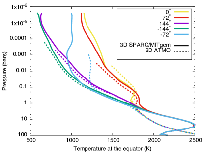
The pressure/temperature structure of the atmosphere can be constrained with 2D and 3D models. A comparison is given in Fig. 4 between the 3D SPARC/MITgcm model and the 2D-ATMO model with the two cases of interior: the hottest one (=10) and the coldest one (=104). For the two values, the upper atmosphere is similar. In this part (pressures less than 1 bar), the agreement between the 2D and the 3D models is quite remarkable since there is no tuning of the 2D model on the 3D model apart from the choice of horizontal wind speed. Since the chemistry and radiative transfer models are independent between the two codes, this agreement is also a sign that convergence between different GCMs and 2D steady-state circulation models can be reached for the pressure/temperature structure at and above the photosphere. As explained in Sect. 3.1, for pressures greater than 1 bar, the different values lead to different temperatures in the deep atmosphere. Because the GCM is not fully converged at pressures larger than 10 bars, it likely produces spurious variations of the deep pressure-temperature profile. The shape of the deep flow structure and its influence in the upper atmospheric dynamics is still an active subject of research (Mayne et al., 2014, 2019; Carone et al., 2019) and out of the scope of this paper. Given that both the GCM and the 2D model produce very similar thermal structure in the observable atmosphere we decided to use the outputs of the 2D model as inputs for the chemical and cloud formation models. We opted for the cold interior model (=104) based on the ground that the planet does not appear to be highly inflated. However, a more thorough investigation of the deep thermal structure on the observable cloud properties (e.g. Powell et al., 2018) will be needed in the future to interpret the observations.
4.2 Chemical composition
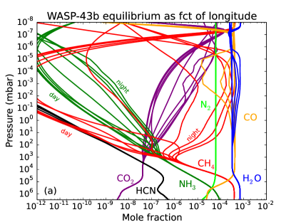
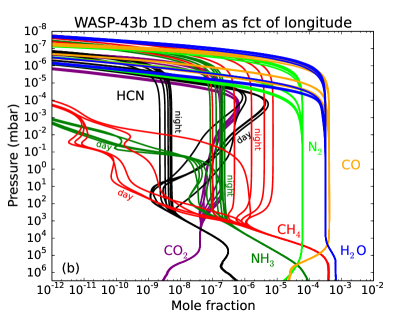
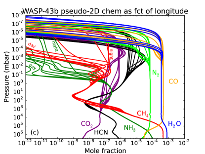
We study the chemical composition of WASP-43b at different longitudes with our 1D and pseudo-2D models. The results are presented in Fig. 5, together with the abundances at thermochemical equilibrium, corresponding to the same longitude-variable thermal structure. In the 1D model, all the longitudes have been computed independently, assuming thermochemical composition as initial composition at each longitude. The different vertical columns don’t interact with each other. In the pseudo-2D model, the longitudes are not independent interacting through horizontal circulation. As we explained in Sect. 3.3, the steady state composition of the substellar point is given as initial condition to the adjacent longitude. There, the evolution of chemical composition is calculated over the amount of time necessary for a parcel of gas to reach the next longitude, and so on.
In all models, as the temperature is identical at each longitude for pressures greater than 103 mbar, we find that species have also the same abundances, corresponding to the thermochemical equilibrium values. The composition varies with longitude above this region, more or less depending on species. For pressures lower than 103 mbar, many of the atmospheric constituents would vary significantly with longitude if the atmosphere remained in thermochemical equilibrium throughout. Particularly noteworthy is the fact that CH4 would be the dominant carbon-bearing constituent at high altitudes on the colder nightside in thermochemical equilibrium, while CH4 would virtually disappear from the dayside and CO would become the dominant carbon-bearing constituent at all altitudes. The 1D kinetic model predicts that vertical quenching will reduce this variation, but there are still several orders of magnitude differences between the abundances of the dayside and that of the nightside. In contrast, the pseudo-2D model predicts much less variation with longitude, particularly in the 0.1–1000 mbar region that is probed at infrared wavelengths. The CO that forms on the hot dayside cannot be chemically converted to CH4 quickly enough on the nightside, before the atmospheric parcels are carried by the zonal winds back to the dayside. These results confirm the findings by Cooper & Showman (2006), Agúndez et al. (2014a), Mendonça et al. (2018b), Drummond et al. (2018a) and Drummond et al. (2018b) that both vertical and horizontal chemical quenching are important in hot Jupiter atmospheres.
Another species whose abundance predicted by our kinetic model is very different from what is expected by thermochemical equilibrium is HCN. At thermochemical equilibrium, this species has the same abundance profile at each longitude, and its abundance decreases with increasing altitude. The 1D kinetic model predicts that this species will be quenched at around 102 mbar, leading to a higher abundance than what is predicted by thermochemical equilibrium on the nightside, and even higher abundance on the dayside thanks to a photochemical production. Note that the quenching pressure we determine with our model is of course highly dependent on the profile we assume. At 102 mbar, is about 4.5107 cm2 s-1. As we said in Sect. 3.3, this parameter is rather uncertain and could vary by several orders of magnitude (typically 106–1012 cm2 s-1 among Parmentier et al. 2013; Agúndez et al. 2014a). Consequently, with these extreme values, the pressure level quenching of HCN could vary between 10 and 105 mbar. In contrast to what has been found with the 1D kinetic model, our pseudo-2D model indicates that the abundance of HCN on the nightside will remain very high and close to that of the dayside thanks to the horizontal circulation, in agreement with Agúndez et al. (2014a). A such high abundance might be detectable thanks to high-resolution spectroscopic observations in the near-infrared coupled to a robust detrending method (Hawker et al., 2018; Cabot et al., 2019). On JWST/MIRI observations, HCN could eventually appear in the 7–8 m band, albeit spectra will probably be dominated by water absorption in this region given the important abundance of H2O in the atmosphere of WASP-43b (Rocchetto et al., 2016).
Similarly to Agúndez et al. (2014a), we find that in addition to vertical quenching due to eddy diffusion, the horizontal circulation leads to horizontal quenching of chemical species. Globally, the atmosphere of WASP-43b has a chemical composition homogenized with longitude to that of the dayside. This is particularly true for pressures larger than 1 mbar, while variations of abundances between the day and nightside still remain at lower pressures.
In summary, the pseudo-2D model suggests that CH4 would be a relatively minor constituent on WASP-43b at all longitudes, that photochemically produced HCN will be more abundant than CH4 in the infrared photosphere of WASP-43b at all longitudes, and that the key spectrally active species H2O and CO will not vary much with longitude on WASP-43b. Benzene (C6H6) is a proxy for photochemical hazes in the pseudo-2D model, and the strong increase in the benzene abundance at nighttime longitudes suggests that refractory hydrocarbon hazes could potentially be produced at night from radicals produced during the daylight hours (e.g. Miller-Ricci Kempton et al., 2012; Morley et al., 2013, 2015). Note that a recent experimental study demonstrates that refractory organic aerosols can be formed in hot exoplanet atmospheres with a C/O ratio higher than solar (Fleury et al., 2019).
Based on these chemical models and because the variation of CH4 with longitude could be observed with MIRI, we ran GCMs assuming chemical equilibrium and assuming a fixed [CH4]/[CO] ratio of 0.001, which is representative of the 2D chemical model in the 0.1-1000 mbar region.
4.3 Cloud coverage
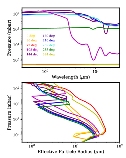
We use the CARMA model to determine the physical and chemical properties of the clouds along different vertical columns at the equator of the planet. Assuming Mie-scattering particles, we calculate the cloud optical depth profile for each longitude from 0.35 to 30 m. Fig. 6 (top) shows the pressure levels at which the total cloud column optical depth (taking into account all cloud species) equals 1, and reveals large differences between the day and night sides. Specifically, the day side temperature profile is such that most of the forsterite (Mg2SiO4) is cold trapped below 100 bars, and although the forsterite condensation curve crosses the temperature profile again at lower pressures, the abundance of Mg there is sufficiently low so as to prevent optically thick clouds from forming (Fig. 7).
On the night side, sufficiently low temperatures allow for the condensation of optically thick MnS and Na2S clouds, such that the optical depth = 1 pressure level is above 0.1 bar blueward of 7 m. As the typical particle sizes of these clouds are 1 to a few m (Fig. 6, bottom), they become optically thin at longer wavelengths, allowing for forsterite clouds to become visible, as shown by the 10 m silicate feature. Note that this forsterite cloud is not the cold-trapped cloud at 100 bars. Instead, because the forsterite condensation curve crosses the temperature profile a second time at higher pressures here than on the day side, there is sufficient Mg to produce an optically thick “upper” cloud even after accounting for cold trapping. The shape of the effective particle radius profiles shown in Fig. 6 (bottom) also reveals this transition in cloud composition with longitude, as particle size tends to increase towards the cloud base due to available condensate vapor supply and size sorting by lofting and sedimentation. For example, while day side profiles are largely smooth, corresponding to the dominance of the forsterite cloud, the night side profiles feature a MnS cloud deck above 1 bar sitting atop the forsterite cloud below (Fig. 7).
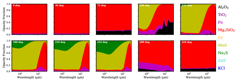
Our results suggest that whether forsterite or enstatite is considered the primary silicate condensate could strongly impact the dayside cloud opacity. As enstatite condenses at lower temperatures (Fig. 3), it would not form a deep cloud at pressures 100 bars on the day side, like forsterite. This lack of cold trapping may result in an optically thick cloud at lower pressures. This is in contrast to the nightside, where forsterite only dominates the cloud opacity at long wavelengths. We therefore expect that, since the cloud base of forsterite is only 50% higher in pressure than enstatite, forsterite will have similar effect on the night side spectra as enstatite. Whether the forsterite or enstatite clouds are cold trapped in the deep atmospheric layers depends on both microphysical behavior of the cloud (studied here), the strength of the vertical mixing and the temperature in the deep atmosphere (Powell et al., 2018). Thorngren et al. (2019) recently predicted a connection between planet equilibrium temperature and their intrinsic flux, suggesting that cold traps on certain hot Jupiters may not exist due to high temperatures in the deep atmosphere. By determining the cloud chemical composition in the nightside of WASP-43b through our JWST/MIRI phase curve observation will provide insights into the presence of a deep cold trap and thus test the predictions from Thorngren et al. (2019).
Our work decouples cloud microphysics from the radiation field and dynamics of the rest of the atmosphere, and thus we cannot treat cloud radiative feedback or cloud advection. Fully coupled 3D models that include cloud microphysics in the form of grain chemistry have been applied to other individual exoplanets in the past, including HD 189733b and HD 209458b, which have similar temperatures to WASP-43b (Helling et al., 2016; Lee et al., 2016; Lines et al., 2018a, b). These works show that the mean particle radii vary between 1-100 m between 0.1 and 100 bars, and that the composition of mixed cloud particles is dominated by enstatite, forsterite, iron, SiO, and SiO2, with forsterite being more abundant than enstatite at most longitudes. This is similar to our results, though we do not consider SiO and SiO2 in our model, while they do not consider sulfide clouds in theirs. Advection tends to smooth out cloud composition differences, which we do not capture in our work. One other major difference between the grain chemistry models and our model is the high abundance of small particles at low pressures in grain chemistry models stemming from high nucleation rates at low pressures. In contrast, nucleation rates are the highest at the cloud base in our model (Gao et al., 2018) owing to the high atmospheric density there, and so we lack a low pressure, small particle population.
To summarize, our results show that, if silicates primarily form forsterite clouds, then the day side of WASP-43b should be cloudless down to 100 bars, while the night side cloud opacity should be dominated by MnS and Na2S clouds shortward of 7 m, and forsterite clouds at longer wavelengths. Cloud particle sizes on the night side at the pressure levels where clouds become opaque are on the order of 1 to a few m. On the other hand, if silicates primarily form enstatite clouds, then the dayside should be cloudier at pressures 100 bars, while the nightside cloud opacity would remain dominated by the sulfide clouds.
4.4 3-D thermal structure
We use our 3D model to calculate the thermal structure of WASP-43b assuming different chemical composition (thermochemical equilibrium and disequilibrium) and cloudy conditions (clear, MnS, and MgSiO3). The temperature structure and CH4 abundances for the cloudless chemical equilibrium and disequilibrium simulations are shown in Fig. 8. From these models, we calculate the corresponding emission spectra at dayside and nightside.
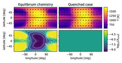
The thermal structure of our cloudless, chemical equilibrium SPARC/MITgcm simulations are very similar to the one presented in Kataria et al. (2015) where the reader can find a thorough description of the atmospheric flows. While Kataria et al. (2015) focused on the effect of TiO, metallicity and drag, we hereafter discuss the role of disequilibrium chemistry and clouds in shaping the nightside spectrum of the planet.
In the case of quenched carbon chemistry ([CH4]/[CO] = 0.001), the dayside is slightly cooler and the nightside is slightly warmer at a given pressure level than for our chemical equilibrium case. However, the differences in the spectra seen in Fig. 9 are mainly due to change in the opacities rather than changes in the thermal structure. On the dayside, where the [CH4]/[CO] ratio is small at chemical equilibrium, our quenched and chemical equilibrium simulations are indistinguishable. On the nightside, the quenching removes the CH4 absorption bands between 3 and 4 m and the ones between 7 and 9 m are weakened in the quenched scenario, leading to a signature detectable by JWST/MIRI. Note that our GCM simulations approximate the [CH4]/[CO] ratio to be constant throughout the atmosphere (horizontally and vertically) for computational reasons, while the pseudo-2D simulations in Section 4.2 as well as 3D simulations of WASP-43b with a simplified chemistry scheme (Mendonça et al., 2018b) find that the methane abundance is homogenized horizontally but decreases with increasing altitude. However, Steinrueck et al. (2018) found that the effect of disequilibrium chemistry on the thermal structure and phase curve is qualitatively similar for different constant [CH4]/[CO] ratios as long as CO is the dominant carbon-bearing species. Therefore, it is likely that the effect of a horizontally homogenized [CH4]/[CO] ratio that decreases with altitude is also qualitatively similar. Our quenched simulation thus still provides a valuable estimate of the effects of disequilibrium chemistry.
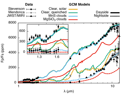
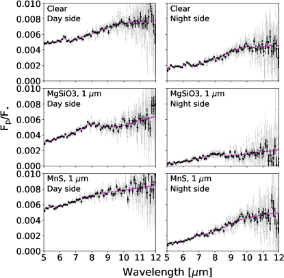
The cloudless simulations were also post-processed with cloud opacities. The post-processing allows for a quick estimate of the strength of potential signature of cloud properties in the emission spectrum without the need to run additional, time-consuming, global circulation models. In Sect. 4.3, we found that the nightside of WASP-43b could be dominated by MnS, Na2S, MgSiO3, and/or Mg2SiO4. Following Parmentier et al. (2016), we explore two possible cloud compositions: MnS and MgSiO3. Forsterite and enstatite having opacities and condensation curves very similar, we chose to include just one of these silicate species. As we found with our microphysical cloud model (Sect. 4.3), the atmosphere of WASP-43b is cool enough for MgSiO3 clouds to cover the whole planet affecting both the dayside and the nightside of the planet. Conversely, MnS clouds can only form on the cooler nightside and thus only affect the nightside’s spectrum. Both MnS and MgSiO3 clouds are able to sufficiently dim the nightside emission spectrum blueward of 5 m in order to match the HST and the Spitzer observations. As shown in Fig. 9, in all our models the nightside flux remains observable with JWST/MIRI, even when the thermal emission is extremely small shortward of 5 m. MnS and MgSiO3 cloud composition could be distinguished spectrally by our JWST/MIRI phase curve observation through the observation of the 10 m absorption band seen in the red models of Fig. 9 (see also Wakeford & Sing, 2015).
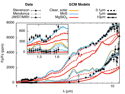
The effect of the cloud particle size is explored in Fig. 10. Assuming that the formation of MnS clouds is limited by the available amount of manganese in a solar-composition atmosphere, the MnS clouds could be either transparent or optically thick in the JWST/MIRI bandpass depending on the size of their particles. Conversely, , if present, should always be optically thick in the MIRI bandpass.
The radiative feedback effect of the clouds in hot Jupiter is a subject of intense research. The amplitude and spatial distribution of the cloud heating is extremely dependent on the cloud model used (e.g. Lee et al., 2016; Roman & Rauscher, 2017; Lines et al., 2018b, 2019; Roman & Rauscher, 2019). In Figure 11 we show the resulting spectrum from a global circulation model incorporating the radiative feedback of MnS clouds. The clouds are opaque up to mbar pressures on the planet nightside and produce a strong greenhouse effect, leading to a warmer nightside and thus a higher nightside flux. Horizontal heat transport from nightside to dayside changes the dayside thermal structure by a thermal inversion, leading to a dayside spectrum dominated by emission features. Qualitatively, any nightside clouds should increase the nightside opacity and warm the atmosphere. The lower the pressure of the cloud photosphere the higher the greenhouse effect of the clouds should. As a consequence, the dayside photosphere, should warm up through heat transport from the nightside to the dayside. The lower the photospheric pressure on the nightside, the larger the warming effect of the clouds on the dayside photosphere. The exemple shown here assumes the highest possible cloud and is therefore likely to overestimate the effect of the nightside cloud on the dayside thermal structure. A deeper cloud will likely have a smaller impact on the dayside spectrum. Overall, because the amplitude and spatial distribution of the cloud heating is extremely dependent on the cloud model used (e.g. Lee et al., 2016; Roman & Rauscher, 2017; Lines et al., 2018b, 2019), we decided to focus the reminder of the paper on the post-processed case by comparing the spectral effect of the clouds for a given thermal structure.
The (cloud-free) quenched simulations are not a good match to existing HST and Spitzer nightside observations. Most likely, this is because the effect of nightside clouds dominates over the effect of disequilibrium chemistry at the wavelengths of existing observations. This situation is qualitatively similar to what Steinrueck et al. (2018) find for HD 189733b. However, quenched chemistry might still be important on the nightside of WASP-43b. We note that during the referee process of this paper, Morello et al. (2019) published a new reduction of the Spitzer observations of WASP-43b. The resulting nightside fluxes lay between those of Stevenson et al. (2017) and Mendonça et al. (2018a).
Also, we note that a new 3D circulation model, elicits for WASP-43b a dynamical regime different from SPARC/MITgcm. Carone et al. (2019) propose that the presence of very deep wind jets down to 700 bar leads to an interruption of superrotation and thus also an interruption of day-to-night side heat transfer. In contrast to that, our SPARC/MITgcm model does not display very deep wind jets. It has uninterrupted superrotation and thus an efficient day-to-night side heat transport. Thus, the Carone et al. (2019)’s model yields colder night sides by several 100 K compared to our model (see also Fig.7 in Carone et al. 2019 for a direct comparison).
5 JWST simulations
We run the JWST simulations following the procedure and assumptions described in Section 3.5 using the different GCM spectra as inputs. Our models predict that there should be clouds on the night-side of WASP-43 b, but other models are consistent with cloud-free night-side atmospheres with deep winds or drag (Carone et al., 2019; Komacek & Showman, 2016). Thus, we perform simulations for cloudy cases and for the cloud-free (“clear”) case to investigate whether they can be distinguished: the cloud-free case should be rejected by the data if the atmosphere is indeed cloudy. Beyond the case study of WASP-43 b, these simulations can inform JWST observation programs of other hot Jupiters, which may have cloudy or clear atmospheres.
The timing and exposure parameters are optimized within PandExo. For these simulations (WASP-43, Kmag = 9.27), the computed parameters are 0.159 second per frame, one frame per group, 83 groups per integration, for a total of 13.36 seconds per integration. This yields 293 integrations during each one eighteenth of the phase curve and 627 in-eclipse integrations including both eclipses. The observing efficiency is 98%. We consider only the 5 – 12 m spectral range. For the in-eclipse observations, the mean electron rate per resolution element at the native MIRI LRS resolution is 5168 e-/s, the median is 2725 e-/s, and it varies from 25229 to 395 e-/s from 5.4 to 12 m. This corresponds to a signal to noise ratio of 13333 at 5.4 m and 536 at 12 m per resolution element. No warnings were issued during the simulations. As expected, these exposure parameters differ slightly from the final ones that are obtained with the JWST Exposure Time Calculator (ETC) and the Astronomer’s Proposal Tool (APT), but this does not affect our results.
Examples of simulations are shown in Fig. 12. At the MIRI LRS native resolution, the wavelength interval between points varies from 0.08 to 0.019 m from 5 to 12 m. We resample the spectra to equal wavelength bins of 0.1 m width. The median uncertainty per spectral bin is 210 ppm, with a notable difference below and above 10 m (with a median uncertainty of 170 ppm and 640 ppm, respectively). Adding a systematic noise floor of 50 ppm (Greene et al., 2016) would not significantly change these uncertainties. Taking the model with a clear atmosphere and quenching as an example, these uncertainties are smaller than the variation between the day- and the night-side by a factor of and below and above 10 m, respectively. They are also smaller than the night side emission by a factor of 14 and 7 below and above 10 m, respectively. Thus, we should be able to detect the night side and day side emission spectra and its variations in longitude. These uncertainties are also smaller than differences between models around specific spectral features, in particular the increased emission around 8 m on the day-side for models with MgSiO3 clouds should be detected. Thus, we should be able to constrain the cloud composition. A detailed retrieval analysis based on these simulations is presented in Section 6.
6 Retrieval
For the atmospheric retrieval of WASP-43b, we consider that the NIRSpec GTO will constrain the H2O mixing ratio before the ERS observations. Thus, in Pyrat Bay we consider a prior based on Greene et al. (2016), while in TauREx we use a uniform prior (1.5–6 for the cloud-free retrieval, 1–1 for the cloudy ones). These priors are consistent with the water abundance determined by our chemical 2D model in the 0.1–1000 mbar region, probed by infrared observations. Since the NIRSpec GTO may not be able to constrain the atmospheric properties on the night side of the planet, we investigate whether the MIRI observations are able to determine: (1) if there are no clouds, is there a disequilibrium-chemistry composition? and (2) if there are clouds, what is their composition?
6.1 Cloud-free Retrieval
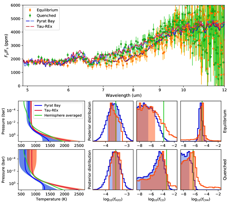
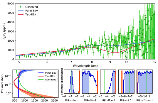
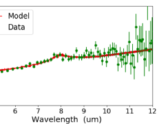
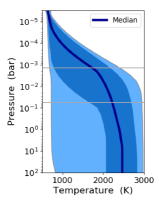
For the night-side cloud-free retrievals, both Pyrat Bay and TauREx reproduce well the simulated data (Fig. 13, top panel) and obtain similar results for the retrieved temperature profile and the molecular abundances (Fig. 13, bottom panels). Note, however, that the temperatures and abundances of the individual cells in the input 3D model span wide ranges, which vary with latitude, longitude, and pressure (see, e.g., Fig. 8). Since the output emission spectrum is not a linear transformation of the input temperature, one must consider the averaged values of the input model as guidelines rather than a strict measure of accuracy.
| Case | Molecule | TauREx | Pyrat Bay |
|---|---|---|---|
| log(H2O) | -3.670.17 | -3.590.31 | |
| Equilibrium | log(CO) | <-5.3 | < -7.0 |
| log(CH4) | -4.820.89 | -5.060.25 | |
| log(H2O) | -3.520.18 | -3.620.27 | |
| Quenched | log(CO) | <-2.9 | < -3.3 |
| log(CH4) | <-5.8 | < -7.2 |
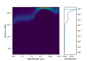
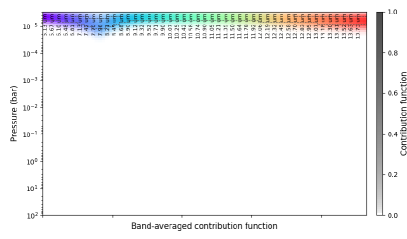
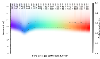
Given the properties of the system, the bulk of the emission from WASP-43b comes from the 0.1–1 bar pressure range. At these altitudes, both codes follow closely the hemisphere-averaged profile of the underlying model; fitting well the non-inverted slope of the temperature profile.
Water is the dominant absorber across the MIRI waveband. Its ubiquitous absorption at all wavelengths shapes the emission spectrum. Both retrievals constrain well the water abundance, aided by the NIRSpec prior (Gaussian for Pyrat Bay, uniform for TauREx).
Methane has its strongest absorption band between 7 and 9 m. Consequently, the larger methane abundance for the equilibrium case over the quenched case produces a markedly lower emission at these wavelengths (more methane concentration leads to stronger absorption, which leads to higher photosphere—at lower temperatures, which leads to lower emission). Both retrievals are able to distinguish between these two cases, producing a precise methane constraint for the equilibrium case (Pyrat Bay obtains a median with 68% HPD (highest-posterior-density) of , whereas TauREx obtains ). The lower concentration of methane in the quenched case leads to wider posteriors and the retrieval is only able to provide an upper limit on the methane concentration.
Carbon monoxide only has a strong band at the shorter edge of the observed spectra (5 m), and thus, its abundance is harder to constrain. In the equilibrium case both retrievals set an upper limit on the CO abundance. In Figure 13, the upper limits of the credible intervals are nearly two orders of magnitude below the averaged CO abundance at 0.3 bar. However, in the input model, CO decreases rapidly with altitude over the probed pressures—from 4 to 4 between 1 and 0.1 bar. Since the retrievals assume a constant-with-altitude profile, the retrieval models require a lower CO abundance to produce the same signal of the input model, which might explain the underestimated retrieved CO values. For the quenched case, both CO posterior distributions peak slightly below the averaged-input.
Table 2 and Figure 13 compare the retrieved abundances and the associated uncertainties for the two cloud-free cases (Equilibrium and Quenched chemistry). Both codes (based on different methods) produce qualitatively similar results for each molecule. The posterior credible intervals are consistent when the molecule is well constrained, whereas they differ by up to two dex when finding upper limits. These results show that both methods are robust. At view of our results, we expect that in a cloud-free case we will be able to distinguish between the equilibrium and quenched scenarios using MIRI phase curve observations of WASP-43b, thanks to the methane absorption band seen between 7 and 9 m.
6.2 Cloudy Retrieval
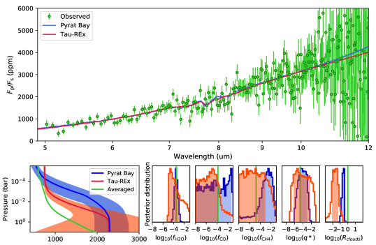
We ran Pyrat Bay and TauREx night-side cloudy retrievals on the 1 m and JWST/MIRI simulated datasets (Figure 12, right-middle and bottom panels). Although both codes retrieved similar best-fit spectra, temperature-profiles, and contribution functions, Pyrat Bay’s TSC cloud model was more successful in retrieving the input condensate particle size, cloud number density, and the location of the cloud deck for the clouds.
To investigate and clouds, TauREx ran “free” retrieval scenarios, while Pyrat Bay ran both “free” and “self-consistent” equilibrium-chemistry retrieval. We chose to include the “self-consistent” scenario, as the clouds in the input synthetic models were post-processed with cloud opacities using the cloudless GCM simulations, in the same way as we add clouds in retrieval (see Section 4.4). For the clouds, both Pyrat Bay and TauREx also ran non-constrained and constrained temperature-profile cases within “free” retrieval, as the data led the parameter exploration to non-physical solutions.
For Pyrat Bay “free” retrieval we used the same setup as in the cloud-free retrieval case (see Sections 3.6 and 6.1) and retrieved the same temperature and pressure parameters (, , , , and ; see Line et al., 2013), with an addition of five new free parameters describing the cloud characteristics (Blecic et al 2019a, in prep.): the cloud extent, , the cloud profile shape, , the condensate mole fraction, , the particle-size distribution, , and the gas number fraction just below the cloud deck, . For the “self-consistent” scenario we retrieved the temperature-pressure parameters together with the aforementioned cloudy parameters, excluding the chemical species parameters. The abundances of the chemical species were produced using the initial implementation of the RATE code (Cubillos et al., 2019), based on Heng & Tsai 5-species solution. We calculated the volume mixing ratio of H2O, CH4, CO, CO2, and C2H2 species given a profile. TauREx uses the same setup as in Sections 3.6 and 6.1, in addition to the cloud prescription and free parameters described in Bohren & Huffman (1983), Appendix A. The free parameters of the model are the condensate mole fraction, , and the peak of the particle-size distribution . For this paper, we use the particle cloud distribution described in Sharp & Burrows (2007).
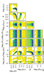
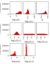
Prior to the Pyrat Bay analysis we ran several different MCMC settings to fully explore the phase space and get the best constraints on the cloud parameters. For all of the tested cases the posterior histograms of some of the cloud parameters were flat with no correlations with other parameters, implying that the data are uninformative about them. Thus, we fixed and excluded them from the exploration ( was fixed to 80, to 0.75, and to 0.0), allowing only the condensate effective particle size, , and the condensate mole fraction, , to be free. This leaves us with the same parameters as TauREx. For the temperature profile in the case, the solution found with TauREx is degenerated between and . We fix this by disabling the contribution of the second visible opacity ().
6.2.1 MnS Clouds
In the MnS case (Figure 14), both Pyrat Bay and TauREx fit well the input spectrum model. While the retrieved temperature profiles are hotter than the hemispheric averaged profile, both profiles converged to similar values at the top of the atmosphere where the contribution functions are located. H2O abundance and cloud mixing ratio were well constrained and closely matching the input value for both codes. As in the cloud-free retrieval, Pyrat Bay used a Gaussian prior on the H2O abundances ((H2O) = -3.52 0.3), while TauREx used an uniform prior (1–1). Pyrat Bay retrieved a H2O abundance to (H2O) = -3.48 0.3, basically the prior value and TauREx retrieved (H2O) = -4.150.71. The retrieved cloud particle sizes have a slightly lower value than the input (Pyrat Bay retrieves m, while TauREx retrieves m). Both codes produced no constraints on the abundance, while CH4 abundances could not be constrained in the TauREx run and has produced a lower limit ((CH4) > -2.4) in the Pyrat Bay run. The retrieved cloud parameters and calculated chemical abundances of the Pyrat Bay “self-consistent” retrieval are nicely matching those of the “free” retrieval. A summary of the retrieved abundances is given in Table 3.
Given the relatively similar results both codes obtained in the cloud-free retrieval case (Sect.6.1), differences seen here between the retrieved parameters’ values within Pyrat Bay and TauREx can be mostly attributed to different cloud parametrization schemes between the two codes: higher complexity of one cloud model compare to the other, different treatment of thermal scattering, larger number of free parameters, more freedom in the shape of the log-normal particle distribution, flexibility in the cloud base location and the shape of the cloud, and possible difference in the resolution of the output models.
TauREx and Pyrat Bay for the MnS clouds cases. There are no uncertainties for the self-consistent runs, which have been performed with Pyrat Bay only.
| Case | Molecule | TauREx | Pyrat Bay |
|---|---|---|---|
| log(H2O) | -4.150.71 | -3.480.30 | |
| Free | log(CO) | < -3 | unconstrained |
| log(CH4) | unconstrained | > -2.4 | |
| log(H2O) | N/A | -3.1 | |
| Self-consistent | log(CO) | N/A | -9.5 |
| (0.1 bar) | log(CH4) | N/A | -3.3 |
6.2.2 MgSiO3 Clouds
For the MgSiO3 clouds, we performed the same “free” retrieval runs as for the MnS clouds. However, in this case, “free” retrievals did not manage to converge to a physically realistic solution for both TauREx and Pyrat Bay. The codes appear to misinterpret the bump at around 8 m as an emission feature, cut the contribution functions at the very top of the atmosphere, and fit the spectrum with a high CH4 abundance and an inverted temperature profile (see Figure 15).
To overcome the encountered issue, we guided the temperature-pressure model to explore only non-inverted solutions in both codes. TauREx was unable to converge to a physical solution, while Pyrat Bay succeeded to get a match between the retrieved temperature and cloud parameters and the input model. In Figure 16 we show the results of this retrieval. To explore only the non-inverted temperature profiles, in Pyrat Bay we fixed and parameters to zero and to values smaller than zero, and let and parameters to be free. The retrieved condensate particle size is 1 m as the input value, cm, and the cloud mole fraction upper limit is around . H2O abundances is again closely matching the Gaussian prior, log10(H2O) = -3.58 0.305, and the contribution functions reveal the location of the cloud at bar, at the same level as the input model. The retrieved best-fit spectrum, median temperature profile, and the condensate particle size ( cm) for the Pyrat Bay “self-consistent” retrieval are almost identical to the constrained “free” retrieval case, with the cloud mole fraction having similar upper limit, but with the contribution functions located at lower pressures ( bar). The chemical abundances values for all MgSiO3 cases are gathered in Table 4. Apart from the prior value retrieved for the water, neither Pyrat Bay nor TauREx are able to provide useful constraints on the chemical abundances. Particularly, in the free retrieval case Pyrat Bay provides a biased measurement of the CH4 abundance. Despite these shortcomings, Pyrat Bay provides a surprisingly good match of the particle size and a realistic upper limit on the cloud height that cannot be obtained with TauREx.
TauREx and Pyrat Bay for the MgSiO3 clouds cases.
| Case | Molecule | TauREx | Pyrat Bay |
|---|---|---|---|
| log(H2O) | not converged | -3.780.29 | |
| Free | log(CO) | not converged | < -1.36 |
| log(CH4) | not converged | > -3.4 | |
| log(H2O) | not converged | -3.580.31 | |
| Constrained | log(CO) | not converged | unconstrained |
| T-P | log(CH4) | not converged | unconstrained |
| log(H2O) | N/A | -3.0 | |
| Self-consistent | log(CO) | N/A | -9.0 |
| (0.1 bar) | log(CH4) | N/A | -3.3 |
In conclusion, based on the cloudy retrieval analysis, distinguishing between cloud-free and cloudy atmospheres in JWST/MIRI data could present a challenge without a careful approach. Even for the 1 m synthetic models with clouds, which show a noticeable silicate feature around 10 m, we saw a degenerate solution with high CH4 abundance, inverted temperature profile and no traces of clouds. The challenge will become even higher for the particle sizes larger than 10 m, as the silicate feature becomes even less pronounced (Wakeford & Sing, 2015).
To overcome this issue, one must closely examine the physical background of the retrieved model (e.g., temperature profile, spectral features seen in emission rather than in absorption, abundances of the retrieved species) and discard non-physical solutions. In addition, the complexity of the underlying parametrized cloud models plays a crucial role. More advanced and realistic cloud models that, for example, include thermal scattering, more freedom in the cloud particle distribution, and the location and shape of the cloud, have higher chances to discard false models and allow Bayesian sampling to land in a realistic phase space. Greene et al. (2016) also points out the importance of the synergy between different instruments on board JWST to obtain wider wavelength coverage and avoid abundances/cloud properties degeneracies. Combining NIRCam, NIRISS, and MIRI instruments, that cover 0.6-11 m range, would be our best way forward (Schlawin et al., 2018). In particular, Mai & Line (2019) show that NIRCam wavelength range ( = 2.5 - 5 m) is critical in inferring atmospheric properties (precise compositional constraints are possible due to the presence of CO and CO2 features at these wavelengths), while NIRISS + MIRI ( = 0.6 - 2.5, 5 - 11 m) are necessary for constraints on cloud parameters (NIRISS is required to constrain the scattering slope at shorter wavelengths, while MIRI is important due to the existence of mid-IR resonance features). Finally, a 2.5D approach such as the one of Irwin et al. (2019) would further improve the ability to retrieve the cloud properties.
Overall, our retrieval models can distinguish between a cloudy and a cloudless nightside, but if the clouds are too thick or have a single-scattering albedo in the infrared that is too large, such as the MgSiO3 case, our state-of-the art retrieval methods have difficulty analysing the complexity of the planned JWST/MIRI observations. If not carefully guided, they can produce biased detection of a high CH4 abundance, regardless of a well-known specific absorption feature at 10 m. More work is needed to leverage the planned observations and quantify the nightside abundances in the presence of nigthside clouds.
7 Conclusions
In order to prepare the future observations of WASP-43b that will be carried out during the JWST Early Release Science Program (PIs: N. Batalha, J. Bean, K. Stevenson; Stevenson et al., 2016; Bean et al., 2018), we performed a series of theoretical models to better understand the atmosphere of this hot Jupiter and predict JWST/MIRI observations. In addition to predictions of the observed spectra, this work allowed us to compare some outputs obtained with our different models, highlighting uncertainties in atmospheric properties and exploring the robustness and weakness of atmospheric retrievals. The key results of this study are:
- The thermal structure and the corresponding spectra found with our 2D radiative transfer code (2D-ATMO) was very similar to that found with our more complex Global Circulation Model (SPARC/MITgcm), despite the two codes being based on different physical approaches. Because the 2D code runs much faster than the GCM, it presents a very good alternative for atmospheric studies that need to be rapidly addressed.
- From a chemical aspect, thanks to our 1D and pseudo-2D chemical models of WASP-43b’s atmosphere, we found that the main constituents after H2/He were CO, H2O and N2. Methane is not expected to be abundant in the layers probed by observations, but HCN, photochemically produced on the dayside, could be the second-most important C-bearing species after CO in these regions.
- Thanks to our microphysical clouds model, we determine that the night side of WASP-43b is probably cloudy (MnS, Na2S, Mg2SiO4/MgSiO3). The cloud coverage of the dayside depends on whether silicates form a deep cloud. This depends on microphysics (e.g. forsterite vs. enstatite formation), atmospheric dynamics (strenght of vertical mixing) and the deep energetics (how hot is the planet interior).
- By simulating the observations and performing a data retrieval, we showed that this full orbit spectroscopic phase curve should allow us to constrain the nightside pressure-temperature structure, and the H2O, CH4, and CO abundances if the atmosphere is not cloudy. We would be able to conclude whether horizontal quenching drives the nightside atmosphere out of chemical equilibrium. If the atmosphere is cloudy we should be able to detect the presence of clouds, differentiate between different cloud chemical composition and constrain the mean particle size with retrieval models that include mie scattering such as Pyrat Bay. However, quantifying the nightside atmospheric composition, thermal structure, and cloud abundance will be more challenging and requires more careful preparation.
References
- Ackerman & Marley (2001) Ackerman, A. S., & Marley, M. S. 2001, ApJ, 556, 872
- Ackerman et al. (1995) Ackerman, A. S., Toon, O. B., & Hobbs, P. V. 1995, J. Geophys. Res., 100, 7121
- Adcroft et al. (2004) Adcroft, A., Campin, J.-M., Hill, C., & Marshall, J. 2004, Monthly Weather Review, 132, 2845
- Agúndez et al. (2014a) Agúndez, M., Parmentier, V., Venot, O., Hersant, F., & Selsis, F. 2014a, A&A, 564, A73
- Agúndez et al. (2012) Agúndez, M., Venot, O., Iro, N., et al. 2012, A&A, 548, A73
- Agúndez et al. (2014b) Agúndez, M., Venot, O., Selsis, F., & Iro, N. 2014b, ApJ, 781, 68
- Allen et al. (1981) Allen, M., Yung, Y. L., & Waters, J. W. 1981, J. Geophys. Res., 86, 3617
- Amundsen et al. (2014) Amundsen, D. S., Baraffe, I., Tremblin, P., et al. 2014, A&A, 564, A59
- Amundsen et al. (2017) Amundsen, D. S., Tremblin, P., Manners, J., Baraffe, I., & Mayne, N. J. 2017, A&A, 598, A97
- Asplund et al. (2009) Asplund, M., Grevesse, N., Sauval, A. J., & Scott, P. 2009, ARA&A, 47, 481
- Barber et al. (2006) Barber, R. J., Tennyson, J., Harris, G. J., & Tolchenov, R. N. 2006, MNRAS, 368, 1087
- Bardeen et al. (2008) Bardeen, C. G., Toon, O. B., Jensen, E. J., Marsh, D. R., & Harvey, V. L. 2008, Journal of Geophysical Research, 113, D17202
- Barth & Toon (2003) Barth, E. L., & Toon, O. B. 2003, Icarus, 162, 94
- Batalha et al. (2017) Batalha, N. E., Mandell, A., Pontoppidan, K., et al. 2017, PASP, 129, 064501
- Bates (1984) Bates, D. R. 1984, Planet. Space Sci., 32, 785
- Baudino et al. (2017) Baudino, J.-L., Molliere, P., Venot, O., et al. 2017, ArXiv e-prints, arXiv:1710.08235 [astro-ph.EP]
- Bean et al. (2018) Bean, J. L., Stevenson, K. B., Batalha, N. M., et al. 2018, Publications of the Astronomical Society of the Pacific, 130, 114402
- Benneke (2015) Benneke, B. 2015, ArXiv e-prints, arXiv:1504.07655
- Bideau-Mehu et al. (1973) Bideau-Mehu, A., Guern, Y., Abjean, R., & Johannin-Gilles, A. 1973, Optics Communications, 9, 432
- Blecic et al. (2014) Blecic, J., Harrington, J., Madhusudhan, N., et al. 2014, ApJ, 781, 116
- Bohren & Huffman (1983) Bohren, C. F., & Huffman, D. R. 1983, Absorption and scattering of light by small particles
- Borysow (2002) Borysow, A. 2002, A&A, 390, 779
- Borysow & Frommhold (1989) Borysow, A., & Frommhold, L. 1989, ApJ, 341, 549
- Borysow et al. (1989) Borysow, A., Frommhold, L., & Moraldi, M. 1989, ApJ, 336, 495
- Borysow et al. (2001) Borysow, A., Jorgensen, U. G., & Fu, Y. 2001, J. Quant. Spec. Radiat. Transf., 68, 235
- Borysow et al. (1988) Borysow, J., Frommhold, L., & Birnbaum, G. 1988, ApJ, 326, 509
- Cabot et al. (2019) Cabot, S. H. C., Madhusudhan, N., Hawker, G. A., & Gandhi, S. 2019, MNRAS, 482, 4422
- Carone et al. (2019) Carone, L., Baeyens, R., Mollière, P., et al. 2019, arXiv e-prints, arXiv:1904.13334
- Castelli & Kurucz (2004) Castelli, F., & Kurucz, R. L. 2004, ArXiv Astrophysics e-prints, astro-ph/0405087
- Cavalié et al. (2017) Cavalié, T., Venot, O., Selsis, F., et al. 2017, Icarus, 291, 1
- Cavalié et al. (2014) Cavalié, T., Moreno, R., Lellouch, E., et al. 2014, A&A, 562, A33
- Charnay et al. (2015) Charnay, B., Meadows, V., & Leconte, J. 2015, ApJ, 813, 15
- Chen et al. (2014) Chen, G., van Boekel, R., Wang, H., et al. 2014, A&A, 563, A40
- Colaprete et al. (1999) Colaprete, A., Toon, O. B., & Magalhães, J. A. 1999, Journal of Geophysical Research, 104, 9043
- Cooper & Showman (2006) Cooper, C. S., & Showman, A. P. 2006, ApJ, 649, 1048
- Cubillos et al. (2017) Cubillos, P., Harrington, J., Loredo, T. J., et al. 2017, AJ, 153, 3
- Cubillos (2017) Cubillos, P. E. 2017, ApJ, 850, 32
- Cubillos et al. (2019) Cubillos, P. E., Blecic, J., & Dobbs-Dixon, I. 2019, ApJ, 872, 111
- Czesla et al. (2013) Czesla, S., Salz, M., Schneider, P. C., & Schmitt, J. H. M. M. 2013, A&A, 560, A17
- Drummond et al. (2018a) Drummond, B., Mayne, N. J., Manners, J., et al. 2018a, ApJ, 869, 28
- Drummond et al. (2016) Drummond, B., Tremblin, P., Baraffe, I., et al. 2016, A&A, 594, A69
- Drummond et al. (2018b) Drummond, B., Mayne, N. J., Manners, J., et al. 2018b, ApJ, 855, L31
- Evans et al. (2017) Evans, T. M., Sing, D. K., Kataria, T., et al. 2017, Nature, 548, 58
- Fegley & Lodders (1994) Fegley, Bruce, J., & Lodders, K. 1994, Icarus, 110, 117
- Feng et al. (2016) Feng, Y. K., Line, M. R., Fortney, J. J., et al. 2016, ApJ, 829, 52
- Feroz et al. (2009) Feroz, F., Hobson, M. P., & Bridges, M. 2009, MNRAS, 398, 1601
- Fleury et al. (2019) Fleury, B., Gudipati, M. S., Henderson, B. L., & Swain, M. 2019, ApJ, 871, 158
- Fortney et al. (2006) Fortney, J. J., Cooper, C. S., Showman, A. P., Marley, M. S., & Freedman, R. S. 2006, ApJ, 652, 746
- Freedman et al. (2014) Freedman, R. S., Lustig-Yaeger, J., Fortney, J. J., et al. 2014, The Astrophysical Journal Supplement Series, 214, 25
- Freedman et al. (2008) Freedman, R. S., Marley, M. S., & Lodders, K. 2008, The Astrophysical Journal Supplement Series, 174, 504
- Gao & Benneke (2018) Gao, P., & Benneke, B. 2018, ArXiv e-prints, arXiv:1807.04924 [astro-ph.EP]
- Gao et al. (2018) Gao, P., Marley, M. S., & Ackerman, A. S. 2018, ApJ, 855, 86
- Gao et al. (2014) Gao, P., Zhang, X., Crisp, D., Bardeen, C. G., & Yung, Y. L. 2014, Icarus, 231, 83
- Gao et al. (2017) Gao, P., Fan, S., Wong, M. L., et al. 2017, Icarus, 287, 116
- Gelman & Rubin (1992) Gelman, A., & Rubin, D. B. 1992, Statistical Science, 7, 457
- Gillon et al. (2012) Gillon, M., Triaud, A. H. M. J., Fortney, J. J., et al. 2012, A&A, 542, A4
- Gordon et al. (2017) Gordon, I. E., Rothman, L. S., Hill, C., et al. 2017, J. Quant. Spec. Radiat. Transf., 203, 3
- Greene et al. (2016) Greene, T. P., Line, M. R., Montero, C., et al. 2016, ApJ, 817, 17
- Guillot & Showman (2002) Guillot, T., & Showman, A. P. 2002, A&A, 385, 156
- Hauschildt et al. (1999) Hauschildt, P. H., Allard, F., & Baron, E. 1999, ApJ, 512, 377
- Hawker et al. (2018) Hawker, G. A., Madhusudhan, N., Cabot, S. H. C., & Gandhi, S. 2018, ApJ, 863, L11
- Hellier et al. (2011) Hellier, C., Anderson, D. R., Collier Cameron, A., et al. 2011, A&A, 535, L7
- Helling & Woitke (2006) Helling, C., & Woitke, P. 2006, Astronomy & Astrophysics, 455, 325
- Helling et al. (2008) Helling, C., Ackerman, A., Allard, F., et al. 2008, Monthly Notices of the Royal Astronomical Society, 391, 1854
- Helling et al. (2016) Helling, C., Lee, G., Dobbs-Dixon, I., et al. 2016, MNRAS, 460, 855
- Heng & Tsai (2016) Heng, K., & Tsai, S.-M. 2016, ApJ, 829, 104
- Hoyer et al. (2016) Hoyer, S., Pallé, E., Dragomir, D., & Murgas, F. 2016, AJ, 151, 137
- Irwin et al. (2019) Irwin, P. G. J., Parmentier, V., Taylor, J., et al. 2019, arXiv e-prints, arXiv:1909.03233 [astro-ph.EP]
- Jacobson & Turco (1994) Jacobson, M. Z., & Turco, R. P. 1994, Atmospheric Environment, 28, 1327
- Jiang et al. (2016) Jiang, I.-G., Lai, C.-Y., Savushkin, A., et al. 2016, AJ, 151, 17
- Kataria et al. (2015) Kataria, T., Showman, A. P., Fortney, J. J., et al. 2015, ApJ, 801, 86
- Kendrew et al. (2015) Kendrew, S., Scheithauer, S., Bouchet, P., et al. 2015, PASP, 127, 623
- Kilpatrick et al. (2018) Kilpatrick, B. M., Cubillos, P. E., Stevenson, K. B., et al. 2018, AJ, 156, 103
- Komacek & Showman (2016) Komacek, T. D., & Showman, A. P. 2016, ApJ, 821, 16
- Kreidberg et al. (2014) Kreidberg, L., Bean, J. L., Désert, J.-M., et al. 2014, ApJ, 793, L27
- Lacis & Oinas (1991) Lacis, A. A., & Oinas, V. 1991, J. Geophys. Res., 96, 9027
- Lecavelier Des Etangs et al. (2008) Lecavelier Des Etangs, A., Pont, F., Vidal-Madjar, A., & Sing, D. 2008, A&A, 481, L83
- Lee et al. (2016) Lee, G., Dobbs-Dixon, I., Helling, C., Bognar, K., & Woitke, P. 2016, A&A, 594, A48
- Lee et al. (2013) Lee, J.-M., Heng, K., & Irwin, P. G. J. 2013, ApJ, 778, 97
- Leggett et al. (2017) Leggett, S. K., Tremblin, P., Esplin, T. L., Luhman, K. L., & Morley, C. V. 2017, ApJ, 842, 118
- Leggett et al. (2016) Leggett, S. K., Tremblin, P., Saumon, D., et al. 2016, ApJ, 824, 2
- Li et al. (2015) Li, G., Gordon, I. E., Rothman, L. S., et al. 2015, ApJS, 216, 15
- Line et al. (2013) Line, M. R., Wolf, A. S., Zhang, X., et al. 2013, ApJ, 775, 137
- Lines et al. (2019) Lines, S., Mayne, N. J., Manners, J., et al. 2019, arXiv e-prints, arXiv:1906.11754
- Lines et al. (2018a) Lines, S., Manners, J., Mayne, N. J., et al. 2018a, MNRAS, 481, 194
- Lines et al. (2018b) Lines, S., Mayne, N. J., Boutle, I. A., et al. 2018b, A&A, 615, A97
- Lodders (1999) Lodders, K. 1999, The Astrophysical Journal, 519, 793
- Lodders (2004) Lodders, K. 2004, ApJ, 611, 587
- Lodders (2010) Lodders, K. 2010, in Principles and perspectives in cosmochemistry (Springer), 379
- Lubow et al. (1997) Lubow, S. H., Tout, C. A., & Livio, M. 1997, ApJ, 484, 866
- Mai & Line (2019) Mai, C., & Line, M. R. 2019, arXiv e-prints, arXiv:1908.10904
- Marley & McKay (1999) Marley, M. S., & McKay, C. P. 1999, Icarus, 138, 268
- Mayne et al. (2019) Mayne, N. J., Drummond, B., Debras, F., et al. 2019, ApJ, 871, 56
- Mayne et al. (2014) Mayne, N. J., Baraffe, I., Acreman, D. M., et al. 2014, A&A, 561, A1
- Mendonça et al. (2018a) Mendonça, J. M., Malik, M., Demory, B.-O., & Heng, K. 2018a, AJ, 155, 150
- Mendonça et al. (2018b) Mendonça, J. M., Tsai, S.-M., Matej, M., Grimm, S. L., & Heng, K. 2018b, ArXiv e-prints, arXiv:1808.00501
- Miguel & Kaltenegger (2014) Miguel, Y., & Kaltenegger, L. 2014, ApJ, 780, 166
- Miller-Ricci Kempton et al. (2012) Miller-Ricci Kempton, E., Zahnle, K., & Fortney, J. J. 2012, ApJ, 745, 3
- Morello et al. (2019) Morello, G., Danielski, C., Dickens, D., Tremblin, P., & Lagage, P. O. 2019, AJ, 157, 205
- Morley et al. (2013) Morley, C. V., Fortney, J. J., Kempton, E. M. R., et al. 2013, ApJ, 775, 33
- Morley et al. (2012) Morley, C. V., Fortney, J. J., Marley, M. S., et al. 2012, The Astrophysical Journal, 756, 172
- Morley et al. (2015) Morley, C. V., Fortney, J. J., Marley, M. S., et al. 2015, ApJ, 815, 110
- Moses (2014) Moses, J. I. 2014, Philosophical Transactions of the Royal Society of London Series A, 372, 20130073
- Moses et al. (2013a) Moses, J. I., Madhusudhan, N., Visscher, C., & Freedman, R. S. 2013a, ApJ, 763, 25
- Moses et al. (2011) Moses, J. I., Visscher, C., Fortney, J. J., et al. 2011, ApJ, 737, 15
- Moses et al. (2013b) Moses, J. I., Line, M. R., Visscher, C., et al. 2013b, ApJ, 777, 34
- Moses et al. (2016) Moses, J. I., Marley, M. S., Zahnle, K., et al. 2016, ApJ, 829, 66
- Mousis et al. (2014) Mousis, O., Fletcher, L. N., Lebreton, J.-P., et al. 2014, Planet. Space Sci., 104, 29
- Murgas et al. (2014) Murgas, F., Pallé, E., Zapatero Osorio, M. R., et al. 2014, A&A, 563, A41
- Naus & Ubachs (2000) Naus, H., & Ubachs, W. 2000, Opt. Lett., 25, 347
- Parmentier et al. (2016) Parmentier, V., Fortney, J. J., Showman, A. P., Morley, C., & Marley, M. S. 2016, ApJ, 828
- Parmentier & Guillot (2014) Parmentier, V., & Guillot, T. 2014, A&A, 562, A133
- Parmentier et al. (2015a) Parmentier, V., Guillot, T., Fortney, J. J., & Marley, M. S. 2015a, A&A, 574, A35
- Parmentier et al. (2015b) Parmentier, V., Showman, A. P., & de Wit, J. 2015b, Experimental Astronomy, 40, 481
- Parmentier et al. (2013) Parmentier, V., Showman, A. P., & Lian, Y. 2013, A&A, 558, A91
- Pine (1992) Pine, A. S. 1992, J. Chem. Phys., 97, 773
- Powell et al. (2018) Powell, D., Zhang, X., Gao, P., & Parmentier, V. 2018, ApJ, 860, 18
- Ricci et al. (2015) Ricci, D., Ramón-Fox, F. G., Ayala-Loera, C., et al. 2015, PASP, 127, 143
- Richard et al. (2012) Richard, C., Gordon, I. E., Rothman, L. S., et al. 2012, J. Quant. Spec. Radiat. Transf., 113, 1276
- Rieke et al. (2015) Rieke, G. H., Wright, G. S., Böker, T., et al. 2015, PASP, 127, 584
- Rocchetto et al. (2016) Rocchetto, M., Waldmann, I. P., Venot, O., Lagage, P.-O., & Tinetti, G. 2016, ApJ, 833, 120
- Roman & Rauscher (2017) Roman, M., & Rauscher, E. 2017, ApJ, 850, 17
- Roman & Rauscher (2019) —. 2019, ApJ, 872, 1
- Rothman et al. (2010) Rothman, L. S., Gordon, I. E., Barber, R. J., et al. 2010, J. Quant. Spec. Radiat. Transf., 111, 2139
- Schlawin et al. (2018) Schlawin, E., Greene, T. P., Line, M., Fortney, J. J., & Rieke, M. 2018, AJ, 156, 40
- Sharp & Burrows (2007) Sharp, C. M., & Burrows, A. 2007, ApJS, 168, 140
- Showman et al. (2010) Showman, A. P., Cho, J. Y.-K., & Menou, K. 2010, Atmospheric Circulation of Exoplanets, ed. S. Seager, 471
- Showman et al. (2009) Showman, A. P., Fortney, J. J., Lian, Y., et al. 2009, ApJ, 699, 564
- Skilling (2006) Skilling, J. 2006, Bayesian Analysis, 1, 833
- Sneep & Ubachs (2005) Sneep, M., & Ubachs, W. 2005, J. Quant. Spec. Radiat. Transf., 92, 293
- Sousa et al. (2018) Sousa, S. G., Adibekyan, V., Delgado-Mena, E., et al. 2018, A&A, 620, A58
- Steinrueck et al. (2018) Steinrueck, M. E., Parmentier, V., Showman, A. P., Lothringer, J. D., & Lupu, R. E. 2018, ArXiv e-prints, arXiv:1808.02011
- Stevenson et al. (2014) Stevenson, K. B., Désert, J.-M., Line, M. R., et al. 2014, Science, 346, 838
- Stevenson et al. (2016) Stevenson, K. B., Lewis, N. K., Bean, J. L., et al. 2016, PASP, 128, 094401
- Stevenson et al. (2017) Stevenson, K. B., Line, M. R., Bean, J. L., et al. 2017, AJ, 153, 68
- Tennyson & Yurchenko (2012) Tennyson, J., & Yurchenko, S. N. 2012, MNRAS, 425, 21
- Tennyson et al. (2016) Tennyson, J., Yurchenko, S. N., Al-Refaie, A. F., et al. 2016, Journal of Molecular Spectroscopy, 327, 73 , new Visions of Spectroscopic Databases, Volume II
- ter Braak & Vrugt (2008) ter Braak, C. J. F., & Vrugt, J. A. 2008, Statistics and Computing, 18, 435
- Thorngren et al. (2019) Thorngren, D., Gao, P., & Fortney, J. J. 2019, ApJ, 884, L6
- Toon & Ackerman (1981) Toon, O. B., & Ackerman, T. P. 1981, Appl. Opt., 20, 3657
- Toon et al. (1988) Toon, O. B., Turco, R. P., Westphal, D., Malone, R., & Liu, M. S. 1988, Journal of the Atmospheric Sciences, 45, 2123
- Tremblin et al. (2016) Tremblin, P., Amundsen, D. S., Chabrier, G., et al. 2016, ApJ, 817, L19
- Tremblin et al. (2015) Tremblin, P., Amundsen, D. S., Mourier, P., et al. 2015, ApJ, 804, L17
- Tremblin et al. (2017a) Tremblin, P., Chabrier, G., Mayne, N. J., et al. 2017a, ApJ, 841, 30
- Tremblin et al. (2017b) Tremblin, P., Chabrier, G., Baraffe, I., et al. 2017b, ArXiv e-prints, arXiv:1710.02640 [astro-ph.SR]
- Tsai et al. (2017) Tsai, S.-M., Lyons, J. R., Grosheintz, L., et al. 2017, ApJS, 228, 20
- Tsiaras et al. (2016) Tsiaras, A., Rocchetto, M., Waldmann, I. P., et al. 2016, ApJ, 820, 99
- Turco et al. (1979) Turco, R. P., Hamill, P., Toon, O. B., Whitten, R. C., & Kiang, C. S. 1979, Journal of the Atmospheric Sciences, 36, 699
- Venot et al. (2014) Venot, O., Agúndez, M., Selsis, F., Tessenyi, M., & Iro, N. 2014, A&A, 562, A51
- Venot et al. (2012) Venot, O., Hébrard, E., Agúndez, M., et al. 2012, A&A, 546, A43
- Venot et al. (2016) Venot, O., Rocchetto, M., Carl, S., Roshni Hashim, A., & Decin, L. 2016, ApJ, 830, 77
- Venot et al. (2013) Venot, O., Fray, N., Bénilan, Y., et al. 2013, A&A, 551, A131
- Visscher et al. (2006) Visscher, C., Lodders, K., & Fegley, Jr., B. 2006, ApJ, 648, 1181
- Visscher et al. (2010) Visscher, C., Lodders, K., & Fegley, Bruce, J. 2010, ApJ, 716, 1060
- Visscher & Moses (2011) Visscher, C., & Moses, J. I. 2011, ApJ, 738, 72
- Wakeford & Sing (2015) Wakeford, H. R., & Sing, D. K. 2015, A&A, 573, A122
- Wakeford et al. (2017) Wakeford, H. R., Sing, D. K., Kataria, T., et al. 2017, Science, 356, 628
- Waldmann et al. (2015a) Waldmann, I. P., Rocchetto, M., Tinetti, G., et al. 2015a, The Astrophysical Journal, 813, 13
- Waldmann et al. (2015b) Waldmann, I. P., Tinetti, G., Rocchetto, M., et al. 2015b, The Astrophysical Journal, 802, 107
- Wang et al. (2016) Wang, D., Lunine, J. I., & Mousis, O. 2016, Icarus, 276, 21
- Wang et al. (2013) Wang, W., van Boekel, R., Madhusudhan, N., et al. 2013, ApJ, 770, 70
- Woods & Rottman (2002) Woods, T. N., & Rottman, G. J. 2002, Washington DC American Geophysical Union Geophysical Monograph Series, 130, 221
- Yurchenko et al. (2018) Yurchenko, S. N., Al-Refaie, A. F., & Tennyson, J. 2018, A&A, 614, A131
- Yurchenko & Tennyson (2014) Yurchenko, S. N., & Tennyson, J. 2014, MNRAS, 440, 1649
- Zhou et al. (2014) Zhou, G., Bayliss, D. D. R., Kedziora-Chudczer, L., et al. 2014, MNRAS, 445, 2746