Invariance principle for
a Potts interface along a wall

Abstract.

We consider nearest-neighbour two-dimensional Potts models, with boundary conditions leading to the presence of an interface along the bottom wall of the box. We show that, after a suitable diffusive scaling, the interface weakly converges to the standard Brownian excursion.

1. Introduction and results

The rigorous understanding of the statistical properties of interfaces in two-dimensional spin systems has raised considerable interest for nearly 50 years.

Early results mostly dealt with the very-low temperature Ising model. The first rigorous result indicating diffusive behavior for the interface in this model was obtained by Gallavotti in 1972 [17]. It was shown in this paper that, at sufficiently low temperature, the interface in a box of linear size $n$ has fluctuations of order $\sqrt{n}$. A description of the internal structure of the interface (in particular the fact that the interface has a bounded intrinsic width, in spite of its unbounded fluctuations) was provided in [4], while a full invariance principle toward a Brownian bridge was proved in [20]. These works were completed by a number of (nonperturbative) exact results in which the profile of expected magnetization was derived in the presence of an interface, see for instance [1]. Extensions of such low-temperature results to other two-dimensional models have been obtained, although a complete theory is still lacking.

The absence of tools to undertake a nonperturbative analysis led to the analysis of similar problems in simpler “effective” settings; see, for instance, [16].

Nevertheless, during the last 20 years, a lot of progress has been made toward extending such results to all temperatures below critical. In particular, a detailed description of the microscopic structure of the interface as well as a proof of an invariance principle were provided in [7, 18] for the Ising model and [8] for the Potts model.

All the above results were concerned with an interface “in the bulk” (that is, an interface crossing an “infinite strip”). For a long time, the understanding of the corresponding properties for an interface located along one of the system’s boundaries remained much more elusive, even in perturbative regimes. The difficulty is that one has to understand how the interface interacts with the boundary and, in particular, exclude pinning of the interface by the wall. It turns out that a rigorous understanding of such issues requires a surprisingly careful analysis. This was undertaken, in a perturbative regime, by Ioffe, Shlosman and Toninelli in [24]. Although restricted to Ising-type interface, the approach they develop is in principle of a rather general nature.

In [11], Dobrushin states convergence of a properly rescaled Ising interface above a wall towards the standard Brownian excursion, for sufficiently low temperatures. The proof is briefly sketched with a reference to the fundamental low-temperature techniques developed in [12]. It is not entirely clear whether a complete rigorous implementation along these lines would indeed follow from the results in [12, Chapter 4] alone (with the simple correction presented in the Appendix of [24]) or whether it would require the full power of [24] in order to control the competition between the entropic repulsion and the interaction between the interface and the wall.

In the present paper, we prove that such an interface, after suitable diffusive scaling, converges to a Brownian excursion, for all temperatures below $T_{c}$ and arbitrary $q$-state Potts models. We bypass a detailed analysis of the interaction between the interface and the wall by combining monotonicity and mixing properties of these models. Lemma 3.1, which should be considered as one of the main technical, and perhaps conceptual, contributions of this paper, implies that in the case of nearest neighbor Potts models on $\mathbb{Z}^{2}$, entropic repulsion of the interface from the wall wins over a possible attraction of the interface by the wall for all temperatures below critical. This result has important ramifications, for instance it plays a crucial role for proving convergence to Ferrari–Spohn diffusions of low-temperature Ising interfaces in the critical prewetting regime [23], or for studying low-temperature 2D Ising metastable states related to the phenomenon of uphill diffusions [9].

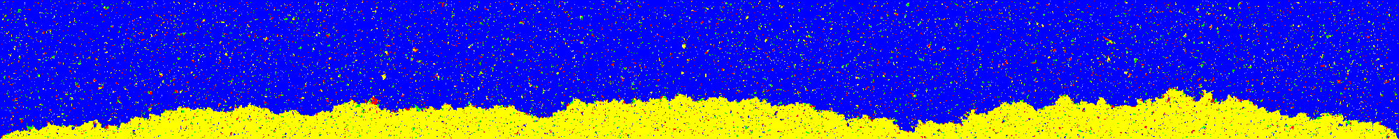
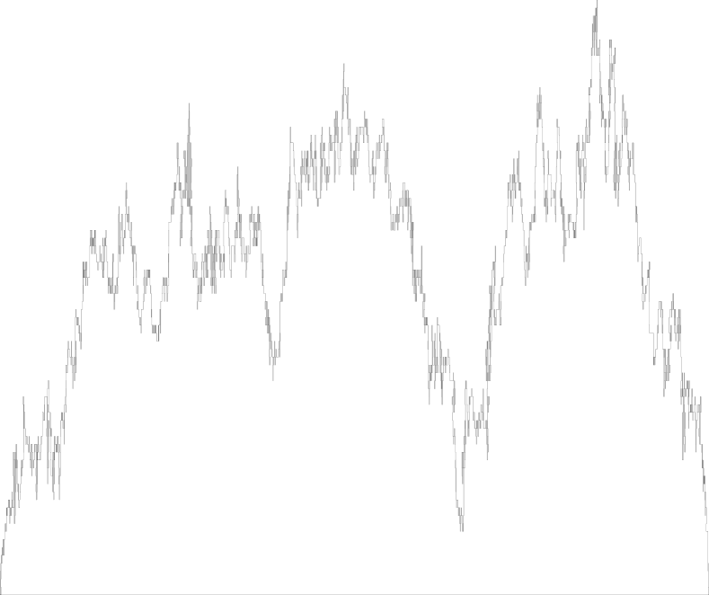
Figure 1. Top left: typical Potts configuration. Bottom left: the corresponding interface. Right: The interface after diffusive scaling.

1.1. Notations and Conventions

We denote $\mathbb{Z}_{+}=\{0,1,2,\dots\}$ the non-negative integers. $C,C_{1},\dots,c,c_{1},\dots$ will denote non-negative constants whose value can change from line to line and that do not depend on the parameters under investigation.

Denote $\mathbb{Z}^{2}=(V_{\mathbb{Z}^{2}}\equiv V,E_{\mathbb{Z}^{2}}\equiv E)$ the graph with vertices $\bigl{\{}i=(i_{1},i_{2})\in\mathbb{R}^{2}\,:\,i_{1},i_{2}\in\mathbb{Z}\bigr{\}}$ and edges between any two vertices $i,j$ at Euclidean distance $1$, which we denote by $i\sim j$. The dual graph $(\mathbb{Z}^{2})^{*}=(V^{*},E^{*})$ has set of vertices $V+(1/2,1/2)$ and edges between any two vertices at distance $1$. There is a natural bijection between $E$ and $E^{*}$, mapping the edge $e=\{i,j\}\in E$ to the unique edge $e^{*}=\{i,j\}^{*}\in E^{*}$ intersecting it; we then say that $e$ and $e^{*}$ are dual to each other.

It will be convenient to see a set $C\subset E$ both as a set of edges and as the subset of $\mathbb{R}^{2}$ given by the union of the closed line segments defined by the edges. We will say that a vertex belongs to $C$ if it is an endpoint of at least one edge of $C$. We denote by $\partial_{\scriptscriptstyle\rm edge}C$ the set of edges in $\mathbb{Z}^{2}\setminus C$ having at least one endpoint in $C$. Those conventions are adapted in a straightforward fashion to $C\subset E^{*}$.

We will say that two vertices $u,v$ are connected in a graph if there exists a path of edges linking them. We denote this property $u\leftrightarrow v$.

1.2. Potts and Random-Cluster Model, Duality

Let $q\geq 2$ be an integer, $\beta\geq 0$, $G=(V_{G},E_{G})$ be a graph, $F=(V_{F},E_{F})\subset G$ be finite and $\alpha\in\{1,\dots,q\}^{V_{G}}$. The $q$-state Potts model on $F$ at inverse temperature $\beta$ with boundary condition $\alpha$ is the probability measure $\mu_{\beta,q,F}^{\alpha}$ on $\{1,\dots,q\}^{V_{F}}$ defined by

$$\mu_{\beta,q,F}^{\alpha}(\sigma)=\frac{1}{\mathcal{Z}_{\beta,q,F}^{\alpha}}\exp\Bigl(\beta\sum_{\{i,j\}\in E_{F}}\mathds{1}_{\{\sigma_{i}=\sigma_{j}\}}+\beta\sum_{\begin{subarray}{c}\{i,j\}\in E_{G}\\ i\in V_{F},j\notin V_{F}\end{subarray}}\mathds{1}_{\{\sigma_{i}=\alpha_{j}\}}\Bigr{missing}),$$

where $\mathcal{Z}_{\beta,q,F}^{\alpha}$ is the normalizing constant.

Let $\beta,G,F$ be as before and $q\geq 1$ be real. Let $\eta\in\{0,1\}^{E_{G}}$. The random-cluster measure on $F$ with edge weight $e^{\beta}-1$, cluster weight $q$ and boundary condition $\eta$ is the probability measure on $\{0,1\}^{E_{F}}$ (identified with the subsets of $E_{F}$) given by

$$\Phi_{\beta,q,F}^{\eta}(\omega)=\frac{1}{Z_{\beta,q,F}^{\eta}}(e^{\beta}-1)^{|\omega|}q^{\kappa_{\eta}(\omega)},$$

where $\kappa_{\eta}(\omega)$ is the number of connected components (clusters) intersecting $V_{F}$ in the graph obtained by taking the graph with vertex set $V_{G}$ and edge set $(\eta\setminus E_{F})\cup\omega$. When omitted from the notation, $\eta$ is assumed to be identically $0$ (free boundary conditions). If the graph $G$ is taken to be $\mathbb{Z}^{2}$, one can define the random-cluster measure dual to $\Phi_{\beta,q,F}^{\eta}$ using the bijection from $\{0,1\}^{E}$ to $\{0,1\}^{E^{*}}$ induced by $\omega^{*}_{e^{*}}=1-\omega_{e}$. The dual measure is then $\Phi_{\beta^{*},q,F^{*}}^{\eta^{*}}$ where $\beta^{*}$ is defined via

$$(e^{\beta}-1)(e^{\beta^{*}}-1)=q.$$ (1)

If $\omega\sim\Phi_{\beta,q,F}^{\eta}$, then $\omega^{*}\sim\Phi_{\beta^{*},q,F^{*}}^{\eta^{*}}$ (see [19]).

As the transition temperature of the Potts model on $\mathbb{Z}^{2}$ is given by $\beta_{\mathrm{\scriptscriptstyle c}}=\log(1+\sqrt{q})$ (the self dual point in the sense of (1), see [3]), one has that $\beta>\beta_{\mathrm{\scriptscriptstyle c}}\implies\beta^{*}<\beta_{\mathrm{\scriptscriptstyle c}}$ and vice versa. Moreover, the transition is sharp: for all $q\geq 1$ and $\beta<\beta_{\mathrm{\scriptscriptstyle c}}(q)$, there exist $C,c>0$ such that $\Phi^{1}_{\beta,q,B_{n}}(0\leftrightarrow\partial B_{n})\leq Ce^{-cn}$ for all $n\geq 1$, where $B_{n}=\{-n,\dots,n\}^{2}$.

One main advantage of the random-cluster model is that it satisfies the FKG lattice condition. The following classical notion will be important for us. An edge $e$ is said to be pivotal for the event $A$ in the configuration $\omega$ if $\mathds{1}_{A}(\omega)+\mathds{1}_{A}(\omega^{\prime})=1$, where the configuration $\omega^{\prime}$ is given by $\omega^{\prime}_{f}=\omega_{f}$ for all $f\neq e$ and $\omega^{\prime}_{e}=1-\omega_{e}$. We denote by $\mathrm{Piv}_{\omega}(A)$ the set of all edges that are pivotal for $A$ in $\omega$. When averaging over $\omega$ under some probability measure, we will often simply write $\mathrm{Piv}(A)$ for the corresponding set of edges.

1.3. Edwards–Sokal Coupling for Interfaces.

We are interested in the behavior of the interface between a pure phase occupying the bulk of the system and a second pure phase located along the boundary. It will be convenient to define the Potts model on $(\mathbb{Z}^{2})^{*}$. Denote $\Lambda_{+}^{*}\equiv\Lambda_{+}^{*}(N)=\bigl{(}[-N+1/2,N-1/2]\times[-1/2,N-1/2]\bigr{)}\cap(\mathbb{Z}^{2})^{*}$. We consider the Potts model on $\Lambda_{+}^{*}$ with boundary condition

$$\alpha^{\pm}_{i}=\begin{cases}1&\text{if }i_{2}<0,\\ 2&\text{if }i_{2}>0.\end{cases}$$

$\mu_{\beta^{*},q,\Lambda_{+}^{*}}^{\alpha^{\pm}}$ is related to the random-cluster model via the Edwards–Sokal coupling: from a configuration $\sigma\in\{1,\dots,q\}^{\Lambda_{+}^{*}}$, one obtains a configuration $\omega^{*}$ on $E^{*}$ by setting (here $e^{*}=\{i,j\}\in E^{*}$ and intersections are between sets of vertices)

• $\omega^{*}_{e^{*}}=1$ if $\{i,j\}\cap\Lambda_{+}^{*}=\varnothing$,

• $\omega^{*}_{e^{*}}=0$ if $\{i,j\}\subset\Lambda_{+}^{*}$ and $\sigma_{i}\neq\sigma_{j}$,

• $\omega^{*}_{e^{*}}=0$ if $\{i,j\}\cap\Lambda_{+}^{*}=\{i\}$ and $\sigma_{i}\neq\alpha_{j}$,

• $\omega^{*}_{e^{*}}=\xi_{e^{*}}$ in the other cases, where $(\xi_{e^{*}})_{e^{*}\in E^{*}}$ is a family of i.i.d. Bernoulli random variables of parameter $1-e^{-\beta}$.

Define then $\omega\in\{0,1\}^{E}$ from $\omega^{*}$ by $\omega_{e}=1-\omega^{*}_{e^{*}}$. One has $\omega\sim\Phi_{\beta,q,\Lambda_{+}}(\,\cdot\,|\,v_{L}\leftrightarrow v_{R})$ where $\Lambda_{+}=\{-N,\dots,N\}\times\{0,\dots,N\}$ and $v_{L}=(-N,0),v_{R}=(N,0)$. We will also denote $\Lambda_{-}=\{-N,\dots,N\}\times\{-1,\dots,-N\}$ .

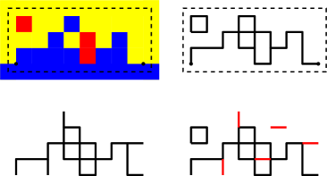
Figure 2. From top left to bottom left in clockwise order: a Potts interface on the dual box; its Peierls contours; the random cluster configuration obtained from it by independently opening nonfrozen edges with probabiity $1-e^{-\beta}$; the cluster we will study.

Remark 1.1.

The way we constructed $\omega$ implies that the Peierls contours between different colors in the Potts configuration are included in $\omega$. Thus, any reasonable notion of the interface between $1$ and $2$ induced by the boundary condition is a subset of the common cluster of $v_{L}$ and $v_{R}$ in $\omega$.

From now on, we will often omit $q$ from the notation (it will be supposed integer and $\geq 2$ when talking about the Potts model and its coupling with the random-cluster model and supposed real and $\geq 1$ when talking about the random-cluster model alone). We will also systematically take $\beta^{*}>\beta_{\mathrm{\scriptscriptstyle c}}(q)>\beta$ and denote by $\Phi$ the (unique) infinite-volume measure. To lighten notations, we will drop the $\beta$-dependency in the proofs (Sections 2, 3 and 4).

1.4. Surface Tension and Wulff Shape

For a direction $s\in\mathbb{S}^{1}$, define the configuration ${\alpha}^{s}\in\{1,2\}^{V^{*}}$ (remember that $V^{*}$ is the set of vertices of the graph $(\mathbb{Z}^{2})^{*}$) by

$${\alpha}^{s}_{i}=\begin{cases}1&\text{ if }i\cdot s>0\\ 2&\text{else}\end{cases},$$

where $\cdot$ denotes the scalar product. The surface tension in the direction $s$ at inverse temperature $\beta^{*}$ is defined as

$$\tau_{\beta^{*}}(s)=-\lim_{N\to\infty}\frac{1}{l_{s}(N)}\log(\frac{\mathcal{Z}_{\beta^{*},\Lambda_{N}^{*}}^{{\alpha}^{s}}}{\mathcal{Z}_{\beta^{*},\Lambda_{N}^{*}}^{1}}),$$

where $\Lambda_{N}^{*}=\bigl{(}[-N+1/2,N-1/2]\times[-N+1/2,N-1/2]\bigr{)}\cap(\mathbb{Z}^{2})^{*}$ and $l_{s}(N)$ is the length of the line segment determined by the intersection of the straight line through $0$ with normal $s$ and the set $[-N,N]^{2}$. It is known that $\tau_{\beta^{*}}(s)>0$ for all $s$ and all $\beta^{*}>\beta_{\mathrm{\scriptscriptstyle c}}(q)$ [14]. In fact, the surface tension can be defined for a rather large class of models in arbitrary dimensions [25] and its homogeneous of order one extension is convex and, therefore, can be represented as the support function of the so-called equilibrium crystal (Wulff) shape ${\mathbf{K}}_{\beta^{*}}$. In two dimensions, the boundary $\partial{\mathbf{K}}_{\beta^{*}}$ is analytic and has a uniformly positive curvature [8] at all sub-critical temperatures $\beta^{*}>\beta_{c}$. The inverse transition temperature $\beta_{\mathrm{\scriptscriptstyle c}}=\beta_{\mathrm{\scriptscriptstyle c}}(q)=\log(1+\sqrt{q})$ can thus be characterized as

$$\beta_{\mathrm{\scriptscriptstyle c}}(q)=\inf\{\beta^{*}\geq 0\,:\,\tau_{\beta^{*}}>0\}.$$

Set $\tau=\tau_{\beta^{*}}\left({\vec{e}_{1}}\right)$ to be the surface tension in the horizontal axis direction $\vec{e}_{1}=(1,0)$. In the sequel, we shall use $\chi=\chi_{\beta^{*}}$ to denote the curvature of ${\mathbf{K}}_{\beta^{*}}$ at its rightmost point $\tau{\vec{e}_{1}}\in\partial{\mathbf{K}}_{\beta^{*}}$.

A direct consequence of the correspondence between the Potts model on $(\mathbb{Z}^{2})^{*}$ at inverse temperature $\beta^{*}$ and the random-cluster model on $\mathbb{Z}^{2}$ at inverse temperature $\beta$ is that

$$\tau=-\lim_{N\to\infty}\frac{1}{2N+1}\log\Phi_{\beta,\Lambda_{N}}(v_{L}\leftrightarrow v_{R})=-\lim_{N\to\infty}\frac{1}{N}\log\Phi_{\beta}\big{(}0\leftrightarrow(N,0)\big{)},$$

where $\Phi_{\beta}$ is the random-cluster distribution on $\mathbb{Z}^{2}$ obtained as the limit of the finite-volume measures on square boxes with $0$ boundary condition.

1.5. Results

We will denote $\Gamma=C_{v_{L},v_{R}}$ the joint cluster of $v_{L},v_{R}$ under $\Phi_{\beta,\Lambda_{+}}(\,\cdot\,|\,v_{L}\leftrightarrow v_{R})$. We also define the upper and lower vertex boundary of $\Gamma$:

$$\Gamma^{+}_{k}=\max\{j:(k,j)\in\Gamma\}\ {\rm and}\ \Gamma^{-}_{k}=\min\{j:(k,j)\in\Gamma\}\ {\rm for}\ k=-N,\dots,N.$$

We will see $\Gamma^{+}$ and $\Gamma^{-}$ as integer-valued random functions on $\{-N,\dots,N\}$.

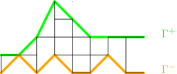
Figure 3. The cluster of Figure 2 and the graphs of the (linear interpolation of the) two associated vertex boundaries $\Gamma^{+}$ and $\Gamma^{-}$.

1.6. Scaling limit of the interface

Let, for $t\in[0,1]$,

$$\hat{\Gamma}^{+}(t)=\frac{1}{\sqrt{N}}{\Gamma^{+}_{-N+\lfloor 2Nt\rfloor}},\qquad\hat{\Gamma}^{-}(t)=\frac{1}{\sqrt{N}}{\Gamma^{-}_{-N+\lfloor 2Nt\rfloor}}.$$ (2)

We are now ready to state the main result of this work.

Theorem 1.1.

Fix ${\beta<\beta_{\mathrm{\scriptscriptstyle c}}(q)}$. Then, for any $\epsilon>0$,

$$\lim_{N\to\infty}\Phi_{\beta,\Lambda_{+}}\bigl{(}\sup_{t\in[0,1]}\bigl{\lvert}\hat{\Gamma}^{+}(t)-\hat{\Gamma}^{-}(t)\bigr{\rvert}>\epsilon\bigm{|}v_{L}\leftrightarrow v_{R}\bigr{)}=0.$$ (3)

Furthermore, under the family of measures $\{\Phi_{\beta,\Lambda_{+}}(\,\cdot\,|\,v_{L}\leftrightarrow v_{R})\}$, the following weak convergence result holds as $N\to\infty$:

$$\hat{\Gamma}^{+}\Rightarrow\sqrt{\chi}\mathfrak{e},$$ (4)

where $\mathfrak{e}:[0,1]\to\mathbb{R}$ is the normalized Brownian excursion and, as before, $\chi=\chi(\beta,q)$ is the curvature of the equilibrium crystal shape $\partial{\mathbf{K}}_{\beta^{*}}$ in the horizontal direction.

1.7. Results in related settings

We describe here a few results that would follow by minor adaptations of our analysis. We state the results in the language of high-temperature random-cluster measures, but there are straightforward reformulations in terms of the low-temperature Potts models. Let $\Lambda_{N}=\{-N,\dots,N\}^{2}$ and let $v_{L},v_{R}$ and $\Gamma=C_{v_{L},v_{R}}$ be as before. Let $\mathcal{L}$ be the set of edges with both endpoints having second coordinate $0$. Define $\Phi_{\beta,J,J^{\prime},\Lambda}$ the random-cluster measure with edge weights $e^{\beta}-1$ in $\Lambda_{+}\setminus\mathcal{L}$, $e^{J\beta}-1$ for edges in $\mathcal{L}$ and $e^{\beta J^{\prime}}-1$ for edges having at least one endpoint in $\{-N,\dots,N\}\times\{-1,\dots,-N\}$. In particular, $\Phi_{\beta,1,0,\Lambda}=\Phi_{\beta,\Lambda_{+}}$ and the case $J^{\prime}=1$ is the defect line setting of [26]. Let $\Gamma^{+}$, $\Gamma^{-}$, $\hat{\Gamma}^{+}$ and $\hat{\Gamma}^{-}$ be defined as before.

Theorem 1.2.

Fix $\beta<\beta_{\mathrm{\scriptscriptstyle c}}(q)$, $0\leq J^{\prime}<1$ and $0\leq J\leq 1$. Then, for any $\epsilon>0$,

$$\lim_{N\to\infty}\Phi_{\beta,J,J^{\prime},\Lambda}\bigl{(}\sup_{t\in[0,1]}\bigl{\lvert}\hat{\Gamma}^{+}(t)-\hat{\Gamma}^{-}(t)\bigr{\rvert}>\epsilon\bigm{|}v_{L}\leftrightarrow v_{R}\bigr{)}=0$$

and

$$\hat{\Gamma}^{+}\Rightarrow\sqrt{\chi}\mathfrak{e},$$

where $\chi$ and $\mathfrak{e}$ are as in Theorem 1.1.

Theorem 1.3.

Fix $\beta<\beta_{\mathrm{\scriptscriptstyle c}}(q)$ and $0\leq J<1$. Then, for any $\epsilon>0$,

$$\lim_{N\to\infty}\Phi_{\beta,J,1,\Lambda}\bigl{(}\sup_{t\in[0,1]}\bigl{\lvert}\hat{\Gamma}^{+}(t)-\hat{\Gamma}^{-}(t)\bigr{\rvert}>\epsilon\bigm{|}v_{L}\leftrightarrow v_{R}\bigr{)}=0$$

and

$$\Psi\Rightarrow\frac{1}{2}\nu^{+}+\frac{1}{2}\nu^{-}$$

where $\Psi$ is the law of $\hat{\Gamma}^{+}$ and $\nu^{\pm}$ are the law of $\pm\sqrt{\chi}\mathfrak{e}$, and the rest is as in Theorem 1.1.

Finally, the results and techniques developed in Sections 3–5 pave the way for proving the following statement (the rather tedious details are omitted; see [6] for the proof of a similar statement):

Theorem 1.4.

Fix $\beta<\beta_{\mathrm{\scriptscriptstyle c}}(q)$. For any pair $(J,J^{\prime})$ satisfying $0\leq J^{\prime}<1$ and $0\leq J\leq 1$ or $J^{\prime}=1$ and $0\leq J<1$, there exists $C\geq 0$ (depending on $\beta,q,J,J^{\prime}$) such that

$$\Phi_{\beta,J,J^{\prime},\Lambda}(v_{L}\leftrightarrow v_{R})=\frac{C}{N^{3/2}}e^{-2\tau N}(1+{\mathsf{o}}_{N}(1)).$$

1.8. Organization of the Paper

In Section 2 we present some results about the geometry of long connections in the infinite-volume random-cluster measure and deduce that typically, under $\Phi_{\beta,\Lambda_{+}}(\,\cdot\,|\,v_{L}\leftrightarrow v_{R})$, the long cluster has the structure of a concatenation of small “irreducible” pieces. Section 3 is devoted to the proof that the long cluster under $\Phi_{\beta,\Lambda_{+}}(\,\cdot\,|\,v_{L}\leftrightarrow v_{R})$ is repulsed far away from the lower boundary of $\Lambda_{+}$. We use this repulsion result in Section 4 to construct a coupling between $\Gamma$ under $\Phi_{\beta,\Lambda_{+}}(\,\cdot\,|\,v_{L}\leftrightarrow v_{R})$ and an effective semi-directed random walk conditioned to stay in the upper half-plane. The latter is studied in Section 5 where an invariance principle to Brownian excursion is proven for a general class of such semi-directed random walks.

2. Diamond Decomposition and Ornstein–Zernike Theory

The main result we will need to import is the Ornstein–Zernike representation of long subcritical clusters derived in [8] and [26]. A random-walk representation of long subcritical clusters under the unique infinite-volume measure $\Phi$ was constructed in [8] in the general framework of Ruelle transfer operator for full shifts. In [26, Section 4] an improved renewal version of [8] was developed. We recall here the main objects and the result we will use.

2.1. Cones and Diamonds

We first define the cones and the associated diamonds:

$$\mathcal{Y}^{\blacktriangleleft}=\{i\in\mathbb{Z}^{2}\,:\,i_{1}\geq\absolutevalue{i_{2}}\},\quad\mathcal{Y}^{\blacktriangleright}=-\mathcal{Y}^{\blacktriangleleft},$$

$$D(u,v)=(u+\mathcal{Y}^{\blacktriangleleft})\cap(v+\mathcal{Y}^{\blacktriangleright}).$$

We will also need, for $\delta>0$, $\mathcal{Y}^{\blacktriangleleft}_{\delta}=\{i\in\mathbb{Z}^{2}\,:\,\delta i_{1}\geq\absolutevalue{i_{2}}\}$. Of course, $\mathcal{Y}^{\blacktriangleleft}=\mathcal{Y}^{\blacktriangleleft}_{1}$.

Let $\gamma=(V_{\gamma},E_{\gamma})$ be a connected subgraph of $\mathbb{Z}^{2}$. We will say that $\gamma$ is:

• Forward-confined if there exists $u\in V_{\gamma}$ such that $V_{\gamma}\subset u+\mathcal{Y}^{\blacktriangleleft}$. When it exists, such a $u$ is unique; we denote it $\mathbf{f}({\gamma})$.

• Backward-confined if there exists $v\in V_{\gamma}$ such that $V_{\gamma}\subset v+\mathcal{Y}^{\blacktriangleright}$. When it exists, such a $v$ is unique; we denote it $\mathbf{b}({\gamma})$.

• Diamond-confined if it is both forward- and backward-confined.

• Irreducible if it is diamond-confined and it is not the concatenation of two other diamond-confined graphs (see below for the definition of concatenation).

We will say that $v\in\gamma$ is a cone-point of $\gamma$ if

$$V_{\gamma}\subset v+(\mathcal{Y}^{\blacktriangleright}\cup\mathcal{Y}^{\blacktriangleleft}).$$

We denote $\textnormal{CPts}(\gamma)$ the set of cone-points of $\gamma$.

We call a graph with a distinguished vertex a marked graph. The distinguished vertex is denoted $v^{*}$. Define

• The sets of confined pieces:

  $$\mathfrak{B}_{L}=\{\gamma\text{ marked backward-confined with }v^{*}=0\},$$

  $$\mathfrak{B}_{R}=\{\gamma\text{ marked forward-confined with }\mathbf{f}(\gamma)=0\},$$

  $$\mathfrak{A}=\{\gamma\text{ diamond-confined with }\mathbf{f}(\gamma)=0\},$$

  $$\mathfrak{A}^{\textnormal{irr}}=\{\gamma\text{ irreducible with }\mathbf{f}(\gamma)=0\}.$$

  We see that $\mathfrak{A}$ could be viewed as a subset of both $\mathfrak{B}_{L}$ (via the marking of $\mathbf{f}(\gamma)$) and $\mathfrak{B}_{R}$ (via the marking of $\mathbf{b}(\gamma)$). To fix ideas we shall, unless stated otherwise, think of $\mathfrak{A}$ as of a subset of $\mathfrak{B}_{L}$, that is, by default the vertex $\mathbf{f}(\gamma)=0$ is marked for any $\gamma\in\mathfrak{A}$.

• The displacement along a piece:

  $$X(\gamma)=(\theta(\gamma),\zeta(\gamma))=\begin{cases}\mathbf{b}(\gamma)&\text{ if }\gamma\in\mathfrak{B}_{L},\ \text{in particular, if $\gamma\in\mathfrak{A}$,}\\ v^{*}&\text{ if }\gamma\in\mathfrak{B}_{R}.\end{cases}$$ (5)

• The concatenation operation: for $\gamma_{1}\in\mathfrak{B}_{L}$ and $\gamma_{2}\in\mathfrak{B}_{R}$ define the concatenation of $\gamma_{2}$ to $\gamma_{1}$ as

  $$\gamma_{1}\circ\gamma_{2}=\gamma_{1}\cup(X(\gamma_{1})+\gamma_{2}).$$

  The concatenation of two graphs in $\mathfrak{A}$ is an element of $\mathfrak{A}$ and the concatenation of a graph in $\mathfrak{A}$ to an element of $\mathfrak{B}_{L}$ is an element of $\mathfrak{B}_{L}$. The displacement along a concatenation is the sum of the displacements along the pieces.

2.2. Ornstein–Zernike Theory for long Clusters in Infinite Volume

Recall that $\tau\vec{e}_{1}\in\partial{\mathbf{K}}_{\beta^{*}}$ is the rightmost point on the boundary of the Wulff shape. It can be informally thought of as the proper drift to stretch phase separation lines in the horizontal direction, see the developments of the Ornstein–Zernike theory in [21, 5, 7, 8, 22, 26]. The main claim we import from [26] is

Theorem 2.1.

There exist $C\geq 0,c>0,\delta>0$ such that one can construct two positive finite measures $\rho_{L},\rho_{R}$ on $\mathfrak{B}_{L}$ and $\mathfrak{B}_{R}$ and a probability measure ${\mathbf{p}}$ on $\mathfrak{A}$ such that, for any point $x{=(x_{1},x_{2})}\in\mathcal{Y}^{\blacktriangleleft}_{\delta}$ and any bounded function $f$ of the cluster of $0$,

$$\Bigl{\lvert}e^{\tau\vec{e}_{1}\cdot x}{\Phi}\bigl{(}f(C_{0,x})\mathds{1}_{\{0\leftrightarrow x\}}\bigr{)}-\\ -\sum_{\gamma_{L},\gamma_{R}}\rho_{L}(\gamma_{L})\rho_{R}(\gamma_{R})\sum_{M\geq 0}\sum_{\gamma_{1},\dots,\gamma_{M}}\mathds{1}_{\{X(\gamma)=x\}}f(\gamma)\prod_{i=1}^{M}\mathbf{p}(\gamma_{i})\Bigr{\rvert}\leq C\|f\|_{\infty}e^{-c\|x\|},$$

where the sums are over $\gamma_{L}\in\mathfrak{B}_{L},\gamma_{R}\in\mathfrak{B}_{R}$ and $\gamma_{i}\in\mathfrak{A}$, such that the displacement along the concatenation $\gamma=\gamma_{L}\circ\gamma_{1}\circ\cdots\circ\gamma_{M}\circ\gamma_{R}$ satisfies $X(\gamma)=x$. Moreover, there exist $C^{\prime}\geq 0,c^{\prime}>0$ such that

$${\max\left\{\rho_{L}(\|X(\gamma_{L})\|\geq l),\rho_{R}(\|X(\gamma_{R})\|\geq l),{\mathbf{p}}(\|X(\gamma_{1})\|\geq l)\right\}\leq C^{\prime}e^{-c^{\prime}l}.}$$ (6)

Remark 2.1.

In particular, Theorem 2.1 implies that, up to exponentially small error, $C_{0,x}$ has a linear (in $\|x\|$) number of cone-points under $\Phi(\,\cdot\,|\,0\leftrightarrow x)$.

2.3. Cone-Points of the Half-Space Clusters

We make here our first use of Theorem 2.1.

Lemma 2.2.

Denoting $\Gamma=C_{v_{L},v_{R}}$. There exist $\rho>0$ and $c>0$ such that

$${\Phi_{\Lambda_{+}}}\bigl{(}\absolutevalue{\textnormal{CPts}(\Gamma)}\leq\rho N\bigm{|}v_{L}\leftrightarrow v_{R}\bigr{)}\leq e^{-cN}.$$ (7)

Moreover, there exist $c>0,C\geq 0$ such that

$${\Phi_{\Lambda_{+}}}\bigl{(}\max_{u,v\in\textnormal{CPts}(\Gamma)}\mathds{1}_{\{\textnormal{CPts}(\Gamma)\cap((u_{1},v_{1})\times\mathbb{Z})=\varnothing\}}|u_{1}-v_{1}|\geq\log(N)^{2}\bigm{|}v_{L}\leftrightarrow v_{R}\bigr{)}\leq\frac{C}{N^{c\log(N)}}.$$ (8)

Note that the event $\left\{\textnormal{CPts}(\Gamma)\cap((u_{1},v_{1})\times\mathbb{Z})=\varnothing\right\}$ above simply means that $v$ and $u$ are successive cone points.

Proof.

By the FKG property of the random-cluster measures, as $\Phi\succcurlyeq\Phi_{\Lambda_{+}}$, one can monotonically couple them (for example using the coupling described in Appendix A). Denote this coupling $\Psi$ and let $(\omega,\eta)$ be a random vector of law $\Psi$ with $\omega\geq\eta$. In particular, for any non-decreasing event $A$ such that $\{\eta\in A\}$, all pivotal edges for $A$ in $\omega$ are also pivotal for $A$ in $\eta$. In the same fashion if $\eta\in\left\{v_{L}\leftrightarrow v_{R}\right\}$, then all the cone-points of $\Gamma(\omega)$ are also cone-points of $\Gamma(\eta)$. Via Remark 2.1, Theorem 2.1 implies that there exist $\rho>0$ and $c>0$ such that

$${\Phi}(\absolutevalue{\textnormal{CPts}(\Gamma)}\leq\rho N,v_{L}\leftrightarrow v_{R})\leq e^{-cN}e^{-2\tau N}.$$

Then, by monotonicity and the previous observation on the inclusion of pivotal edges,

$$\Phi_{\Lambda_{+}}\bigl{(}\absolutevalue{\textnormal{CPts}(\Gamma)}\leq\rho N,v_{L}\leftrightarrow v_{R}\bigr{)}\leq\Phi(\absolutevalue{\textnormal{CPts}(\Gamma)}\leq\rho N,v_{L}\leftrightarrow v_{R}),$$

implying (7) as $\Phi_{\Lambda_{+}}(v_{L}\leftrightarrow v_{R})=e^{-2\tau N(1+{\mathsf{o}}(1))}$. Indeed,

$$\Phi_{\Lambda_{+}}\bigl{(}\absolutevalue{\textnormal{CPts}(\Gamma)}\leq\rho N\bigm{|}v_{L}\leftrightarrow v_{R}\bigr{)} =\frac{\Phi_{\Lambda_{+}}\bigl{(}\absolutevalue{\textnormal{CPts}(\Gamma)}\leq\rho N,v_{L}\leftrightarrow v_{R}\bigr{)}}{\Phi_{\Lambda_{+}}\bigl{(}v_{L}\leftrightarrow v_{R}\bigr{)}}$$

$$\leq\frac{e^{-cN}e^{-2\tau N}}{e^{-2\tau N(1+{\mathsf{o}}(1))}}\leq e^{-cN/2},$$

for $N$ large enough. To get (8), let $w_{1},\dots,w_{m}$ be the first coordinate of the cone-points of $\Gamma(\omega)$, ordered from left to right, and let $l_{i}=w_{i+1}-w_{i},i=1,\dots,m-1$. Denote by $w_{j}^{\prime}$, $m^{\prime}$ and $l_{j}^{\prime}$ the corresponding quantities for $\Gamma(\eta)$. The left-hand side of (8) becomes

$$\frac{\Psi\bigl{(}\max_{j\in\{1,\dots,m^{\prime}\}}l_{j}^{\prime}\geq\log(N)^{2},v_{L}\xleftrightarrow{\eta}v_{R}\bigr{)}}{\Phi_{\Lambda_{+}}(v_{L}\leftrightarrow v_{R})}.$$

Now, as the cone-points of $\Gamma(\omega)$ are included in the cone-points of $\Gamma(\eta)$,

$$\max_{j\in\{1,\dots,m^{\prime}\}}l_{j}^{\prime}\leq\max_{i\in\{1,\dots,m\}}l_{i}.$$

Notice that both $\Gamma(\omega)$ and $\Gamma(\eta)$ are well defined as $\eta\in\{v_{L}\leftrightarrow v_{R}\}$ and $\omega\geq\eta$. Using the lower bound $\Phi_{\Lambda_{+}}(v_{L}\leftrightarrow v_{R})\geq CN^{-3/2}e^{-2\tau N}$ from Lemma 3.4 and the bound $\Phi(v_{L}\leftrightarrow v_{R})\leq e^{-2\tau N}$, one obtains

$$\frac{\Psi\Bigl{(}\displaystyle\max_{j\in\{1,\dots,m^{\prime}\}}l_{j}^{\prime}\geq\log(N)^{2},v_{L}\xleftrightarrow{\eta}v_{R}\Bigr{)}}{\Phi_{\Lambda_{+}}(v_{L}\leftrightarrow v_{R})} \leq\frac{\Psi\Bigl{(}\displaystyle\max_{i\in\{1,\dots,m\}}l_{i}\geq\log(N)^{2},v_{L}\xleftrightarrow{\omega}v_{R}\Bigr{)}}{CN^{-3/2}e^{-2\tau N}}$$

$$\leq C^{-1}N^{3/2}\Phi\bigl{(}\max_{i\in\{1,\dots,m\}}l_{i}\geq\log(N)^{2}\bigm{|}v_{L}\leftrightarrow v_{R}\bigr{)}.$$

The bound in (8) thus follows from (6) and standard estimates on the maximum of an i.i.d. family. ∎

For future use, it is convenient to reformulate Lemma 2.2 as follows:

Corollary 2.3.

There exist $\rho>0$, $C>0$ and $c>0$ such that the following statements hold for all $N$ sufficiently large:

1. Up to an event of probability at most $e^{-cN}$ under $\Phi_{\Lambda_{+}}(\,\cdot\,|\,v_{L}\leftrightarrow v_{R})$, the open cluster $C_{v_{L},v_{R}}$ admits an irreducible decomposition

   $$C_{v_{L},v_{R}}=\gamma_{L}\circ\gamma_{1}\circ\dots\circ\gamma_{k}\circ\gamma_{R},$$ (9)

   with $\gamma_{L}\in\mathfrak{B}_{L},\gamma_{R}\in\mathfrak{B}_{R}$ and with at least $k\geq\rho N$ irreducible pieces $\gamma_{1},\dots,\gamma_{k}\in\mathfrak{A}^{\textnormal{irr}}$.

2. Up to an event of probability at most $\frac{C}{N^{c\log(N)}}$ under $\Phi_{\Lambda_{+}}(\,\cdot\,|\,v_{L}\leftrightarrow v_{R})$, the irreducible pieces (viewed as connected subgraphs of the graph $\mathbb{Z}^{2}$) in the decomposition (9) satisfy:

   $$\max\{\operatorname{diam}(\gamma_{L}),\operatorname{diam}(\gamma_{1}),\dots,\operatorname{diam}(\gamma_{k}),\operatorname{diam}(\gamma_{R})\}\leq(\log N)^{2},$$ (10)

   where $\operatorname{diam}(A)$ is the Euclidean diameter of a set $A\subset\mathbb{R}^{2}$.

3. Entropic Repulsion

3.1. A Rough Upper Bound

We will use the coupling constructed in Appendix A. As in Appendix A, let $\Phi_{a,\Lambda}$ to denote the random-cluster measure with weight $e^{\beta}-1$ on edges in $\Lambda_{+}$ and weight $a$ on edges with an endpoint in $\Lambda_{-}$. We denote by $\Psi$ the coupling between $\Phi_{0,\Lambda}=\Phi_{\Lambda_{+}}$ and $\Phi_{e^{\beta}-1,\Lambda}=\Phi_{\Lambda}$.

Lemma 3.1.

For any ${\mathsf{u}},{\mathsf{v}}\in\Lambda_{+}$ and $0\leq a<e^{\beta}-1$,

$$\Phi_{a,\Lambda_{+}}({\mathsf{u}}\leftrightarrow{\mathsf{v}})\leq\Phi\Bigl{(}\mathds{1}_{\{{\mathsf{u}}\leftrightarrow{\mathsf{v}}\}}\bigl{(}1-\epsilon(a)\bigr{)}^{|\mathrm{Piv}({\mathsf{u}}\leftrightarrow{\mathsf{v}})\cap\Lambda_{-}|}\Bigr{)},$$ (11)

where $\Phi$ is the random-cluster measure on $\mathbb{Z}^{2}$ with edge weight $e^{\beta}-1$ and $\epsilon(a)=\frac{e^{\beta}-1-a}{(e^{\beta}-1+q)(e^{\beta}-1)}$.

Proof.

Let $(\omega,\eta)\sim\Psi$ be as in the Appendix ($\omega\sim\Phi_{\Lambda}$). Using the monotonicity of $\Psi$,

$$\Phi_{a,\Lambda_{+}}({\mathsf{u}}\leftrightarrow{\mathsf{v}}) =\Psi\bigl{(}\eta\in\{{\mathsf{u}}\leftrightarrow{\mathsf{v}}\}\bigr{)}$$ (12)

$$=\Psi\bigl{(}\eta,\omega\in\{{\mathsf{u}}\leftrightarrow{\mathsf{v}}\}\bigr{)}$$

$$=\sum_{\begin{subarray}{c}w\in\{0,1\}^{E_{\Lambda}}\\ w\in\{{\mathsf{u}}\leftrightarrow{\mathsf{v}}\}\end{subarray}}\Psi\bigl{(}\omega=w,\eta\in\{{\mathsf{u}}\leftrightarrow{\mathsf{v}}\}\bigr{)}$$

$$\leq\sum_{\begin{subarray}{c}w\in\{0,1\}^{E_{\Lambda}}\\ w\in\{{\mathsf{u}}\leftrightarrow{\mathsf{v}}\}\end{subarray}}\Psi\bigl{(}\omega=w,\eta_{e}=1\ \forall e\in\mathrm{Piv}_{w}({\mathsf{u}}\leftrightarrow{\mathsf{v}})\cap\Lambda_{-}\bigr{)}$$

$$\leq\sum_{\begin{subarray}{c}w\in\{0,1\}^{E_{\Lambda}}\\ w\in\{{\mathsf{u}}\leftrightarrow{\mathsf{v}}\}\end{subarray}}(1-\epsilon)^{|\mathrm{Piv}_{w}({\mathsf{u}}\leftrightarrow{\mathsf{v}})\cap\Lambda_{-}|}\Phi_{\Lambda}(\omega=w)$$

$$=\Phi_{\Lambda}\Bigl{(}\mathds{1}_{\{{\mathsf{u}}\leftrightarrow{\mathsf{v}}\}}(1-\epsilon)^{|\mathrm{Piv}({\mathsf{u}}\leftrightarrow{\mathsf{v}})\cap\Lambda_{-}|}\Bigr{)}.$$

The first inequality is inclusion of events and the second one is (78) with $\epsilon=\epsilon(a)=\frac{e^{\beta}-1-a}{(e^{\beta}-1+q)(e^{\beta}-1)}$. Now, as $1>\epsilon>0$, $\mathds{1}_{\{{\mathsf{u}}\leftrightarrow{\mathsf{v}}\}}(1-\epsilon)^{|\mathrm{Piv}({\mathsf{u}}\leftrightarrow{\mathsf{v}})\cap\Lambda_{-}|}$ is a nondecreasing function (opening an edge can only decrease the number of pivotal once the event is satisfied). Thus, monotonicity of random-cluster measure implies

$$\Phi_{\Lambda}\Bigl{(}\mathds{1}_{\{{\mathsf{u}}\leftrightarrow{\mathsf{v}}\}}(1-\epsilon)^{|\mathrm{Piv}({\mathsf{u}}\leftrightarrow{\mathsf{v}})\cap\Lambda_{-}|}\Bigr{)}\leq\Phi\Bigl{(}\mathds{1}_{\{{\mathsf{u}}\leftrightarrow{\mathsf{v}}\}}(1-\epsilon)^{|\mathrm{Piv}({\mathsf{u}}\leftrightarrow{\mathsf{v}})\cap\Lambda_{-}|}\Bigr{)}.\qed$$

Remark 3.1.

In the case of the wall ($a=0$), one has the following simplification: since the function $\eta\mapsto\mathds{1}_{\{{\mathsf{u}}\leftrightarrow{\mathsf{v}};\mathrm{Piv}({\mathsf{u}}\leftrightarrow{\mathsf{v}})\cap\Lambda_{-}=\varnothing\}}(\eta)$ is non-decreasing, one could have used instead

$$\Phi_{\Lambda_{+}}(u\leftrightarrow v) =\Phi_{\Lambda_{+}}(u\leftrightarrow v,\mathrm{Piv}(u\leftrightarrow v)\cap\Lambda_{-}=\varnothing)$$

$$\leq\Phi_{\Lambda}\bigl{(}u\leftrightarrow v,\mathrm{Piv}(u\leftrightarrow v)\cap\Lambda_{-}=\varnothing\bigr{)}.$$

We will however work with (11), as we want to keep the proof straightforwardly adaptable to the case of Theorem 1.2.

Lemma 3.2.

There exists $c\geq 0$ such that, for any ${\mathsf{u}}=(k,u),{\mathsf{v}}=(k+m,v)\in\Lambda_{+}$ with $m$ large enough and $u,v\leq\sqrt{m}$,

$$e^{\tau m}\Phi_{\Lambda_{+}}({\mathsf{u}}\leftrightarrow{\mathsf{v}})\leq\frac{c(1+u)(1+v)}{m^{3/2}}.$$ (13)

The proof of Lemma 3.2 relies on effective random walk estimates and it is relegated to Subsection 5.3.

3.2. A Rough Lower Bound

Lemma 3.3.

For any $u,v\in\Lambda_{+}$,

$$\Phi_{\Lambda_{+}}(u\leftrightarrow v)\geq\Phi\bigl{(}C_{u}\subset\Lambda_{+},\,u\leftrightarrow v\bigr{)}.$$

Proof.

$$\Phi_{\Lambda_{+}}(u\leftrightarrow v) =\sum_{\begin{subarray}{c}C\subset\Lambda_{+}\\ C\ni u,v\end{subarray}}\Phi_{\Lambda_{+}}\bigl{(}C_{u}=C\bigr{)}$$

$$=\sum_{C\ni u,v}\mathds{1}_{\{C\subset\Lambda_{+}\}}\Phi_{C}\bigl{(}C\ \textnormal{ open}\bigr{)}\Phi_{\Lambda_{+}}\bigl{(}\partial_{\scriptscriptstyle\rm edge}C\ \textnormal{ closed}\bigr{)}$$

$$\geq\sum_{C\ni u,v}\mathds{1}_{\{C\subset\Lambda_{+}\}}\Phi_{C}\bigl{(}C\ \textnormal{ open}\bigr{)}\Phi\bigl{(}\partial_{\scriptscriptstyle\rm edge}C\ \textnormal{ closed}\bigr{)}$$

$$=\Phi\bigl{(}C_{u}\subset\Lambda_{+},\,u\leftrightarrow v\bigr{)},$$

where the sums are over $C$ connected and the inequality is an application of FKG. ∎

From this inequality and Theorem 2.1, one can deduce the following

Lemma 3.4.

There exists a constant $c>0$ such that, for all $N>0$,

$$\Phi_{\Lambda_{+}}(v_{L}\leftrightarrow v_{R})\geq c\,N^{-3/2}e^{-2\tau N}.$$ (14)

The proof of Lemma 3.4 also relies on effective random walk estimates and it is relegated to Subsection 5.4.

3.3. Bootstrapping

We start by proving a BK-type inequality for a certain type of events.

Lemma 3.5.

Let $G=(V_{G},E_{G})$ be a graph and let $F=(V_{F},E_{F})$ be a finite subgraph of $G$. Let $\eta\in\{0,1\}^{E_{G}}$. Denote $\Phi_{F}^{\eta}$ the random-cluster measure on $E_{F}$ with edge weight $e^{\beta}-1\geq 0$, cluster weight $q\geq 1$ and boundary condition $\eta$. For $u,v\in V_{F}$ and $e\in E_{F}$, denote $A_{e}(u,v)$ the event that there exists an open path from $u$ to $v$ not using $e$. Then, for any $e=\{i,j\}\in E_{F}$ and any $x,y\in V_{F}$,

$$\Phi_{F}^{\eta}\bigl{(}A_{e}(x,i),A_{e}(j,y),\,\omega_{e}=1,\,e\in\mathrm{Piv}(x\leftrightarrow y)\bigr{)}\leq e^{\beta}\Phi_{F}^{\eta}\bigl{(}x\leftrightarrow i\bigr{)}\Phi_{F}^{\eta}\bigl{(}i\leftrightarrow y\bigr{)}.$$ (15)

Proof.

First notice that

$$\Phi_{F}^{\eta}\bigl{(}A_{e}(x,i),\,A_{e}(j,y),\,\omega_{e}=1,\,e\in\mathrm{Piv}(x\leftrightarrow y)\bigr{)}=\\ =\frac{e^{\beta}-1}{q}\Phi_{F}^{\eta}\bigl{(}A_{e}(x,i),\,A_{e}(j,y),\,\omega_{e}=0,\,e\in\mathrm{Piv}(x\leftrightarrow y)\bigr{)}.$$ (16)

Summing over the possible realizations of the cluster of $x$ and $i$,

$$\Phi_{F}^{\eta}\bigl{(}A_{e}(x,i), \,A_{e}(j,y),\,\omega_{e}=0,\,e\in\mathrm{Piv}(x\leftrightarrow y)\bigr{)}=$$

$$=\sum_{\begin{subarray}{c}C\ni x,i,\,C\not\ni j,y\\ \partial_{\scriptscriptstyle\rm edge}C\ni e\end{subarray}}\Phi_{F}^{\eta}\bigl{(}C\textnormal{ open},\,\partial_{\scriptscriptstyle\rm edge}C\textnormal{ closed}\bigr{)}\Phi_{F}^{\eta}\bigl{(}j\leftrightarrow y\bigm{|}\partial_{\scriptscriptstyle\rm edge}C\textnormal{ closed}\bigr{)}$$

$$\leq\Phi_{F}^{\eta}(j\leftrightarrow y)\sum_{C\ni x,i}\Phi_{F}^{\eta}\bigl{(}C\textnormal{ open},\,\partial_{\scriptscriptstyle\rm edge}C\textnormal{ closed}\bigr{)}$$

$$=\frac{\Phi_{F}^{\eta}(j\leftrightarrow y)\Phi_{F}^{\eta}(\omega_{e}=1)}{\Phi_{F}^{\eta}(\omega_{e}=1)}\Phi_{F}^{\eta}(i\leftrightarrow x)\leq\frac{e^{\beta}-1+q}{e^{\beta}-1}\Phi_{F}^{\eta}(i\leftrightarrow y)\Phi_{F}^{\eta}(i\leftrightarrow x).$$

The first inequality is FKG and the second is FKG and finite energy (that is, the fact that the probability for an edge to be open, conditionnally on all the other edges, is uniformly bounded away from $0$ and $1$). Plugging this into (16) yields the result. ∎

This Lemma will prove useful as cone-points events imply the events in the left-hand side of (15). First, by (8) and the definition of $\mathcal{Y}^{\blacktriangleleft}$, we have

$$\Phi_{\Lambda_{+}}\bigl{(}d_{\mathrm{H}}(C_{v_{L},v_{R}},\,\textnormal{CPts}(C_{v_{L},v_{R}}))\leq(\log N)^{2}\bigm{|}v_{L}\leftrightarrow v_{R}\bigr{)}\xrightarrow{N\to\infty}1,$$ (17)

where $d_{\mathrm{H}}$ denotes the Hausdorff distance. Moreover, this convergence is super-polynomial (the error decays faster than any negative power of $N$).

Let $\epsilon>0$, define

$$\Delta\equiv\Delta(N,\epsilon)=[-N+2N^{8\epsilon},N-2N^{8\epsilon}]\times[0,N^{\epsilon}],$$ (18)

$$\tilde{\Delta}\equiv\tilde{\Delta}(N,\epsilon)=[-N+N^{8\epsilon},N-N^{8\epsilon}]\times[0,2N^{\epsilon}].$$

Lemma 3.6.

For any $\epsilon\in(0,1/8)$, there exists $C\geq 0$ such that

$$\Phi_{\Lambda_{+}}\bigl{(}C_{v_{L},v_{R}}\cap\Delta\neq\varnothing\bigm{|}v_{L}\leftrightarrow v_{R}\bigr{)}\leq CN^{-\epsilon}.$$ (19)

Proof.

By (17), we can suppose that $d_{\mathrm{H}}(C_{v_{L},v_{R}},\textnormal{CPts}(C_{v_{L},v_{R}}))\leq(\log N)^{2}$. Under this event, $\{C_{v_{L},v_{R}}\cap\Delta\neq\varnothing\}$ implies $\{\textnormal{CPts}(C_{v_{L},v_{R}})\cap\tilde{\Delta}\neq\varnothing\}$ (for $N$ large enough). By a union bound, the probability of the latter is bounded from above by

$$\Phi_{\Lambda_{+}}\bigl{(}\textnormal{CPts}(C_{v_{L},v_{R}})\cap\tilde{\Delta}\neq\varnothing \bigm{|}v_{L}\leftrightarrow v_{R}\bigr{)}\leq$$ (20)

$$\leq\sum_{u\in\tilde{\Delta}}\frac{\Phi_{\Lambda_{+}}\bigl{(}u\in\textnormal{CPts}(C_{v_{L},v_{R}}),\,v_{L}\leftrightarrow v_{R}\bigr{)}}{\Phi_{\Lambda_{+}}\bigl{(}v_{L}\leftrightarrow v_{R}\bigr{)}}$$

$$\leq Ce^{2\tau N}{N}^{3/2}\sum_{u\in\tilde{\Delta}}e^{\beta}\Phi_{\Lambda_{+}}\bigl{(}v_{L}\leftrightarrow u\bigr{)}\Phi_{\Lambda_{+}}\bigl{(}u\leftrightarrow v_{R}\bigr{)}$$

$$\leq C{N}^{3/2}\sum_{k=N^{8\epsilon}}^{2N-N^{8\epsilon}}\sum_{l=0}^{2N^{\epsilon}}(1+l)^{2}k^{-3/2}(2N-k)^{-3/2}$$

$$\leq CN^{3\epsilon}\sum_{k=N^{8\epsilon}}^{N/2}k^{-3/2}\leq CN^{3\epsilon}N^{-4\epsilon}\xrightarrow{N\to\infty}0,$$

where the first line follows from a union bound, the second one from (15) (since by construction if $u\in\textnormal{CPts}(C_{v_{L},v_{R}})$, then the bonds $\langle u-\mathsf{e}_{1},u\rangle$ and $\langle u,u+\mathsf{e}_{1}\rangle$ are pivotal for $\left\{v_{L}\leftrightarrow v_{R}\right\}$) and Lemma 3.4, and the third one from Lemma 3.2. By convention the constant $C$ is updated at each line. ∎

4. Proof of Theorems 1.1, 1.2 and 1.3

We focus on the proof of Theorem 1.1. The necessary adaptations needed to prove the other two theorems are sketched in Section 4.5.

Throughout this Section we fix $\epsilon\in(0,1/16)$, which is used to define the rectangle $\Delta$ in (18) and, subsequently, shows up in the statement of the entropic repulsion Lemma 3.6. To facilitate notation we set $\delta=8\epsilon\in(0,1/2)$.

4.1. Reduction to infinite volume quantities

Consider the irreducible decomposition (9). In view of Corollary 2.3, we may restrict attention to clusters $C_{v_{L},v_{R}}$ which contain cone-points in any vertical slab of width $(\log N)^{2}$. In the sequel, we shall use $\mathcal{S}_{a,b}$ for the vertical slab through the vertices $(a,0)$ and $(b,0)$.

Let ${\mathsf{u}}_{L}$ be the left-most cone-point of $C_{v_{L},v_{R}}$ in $\mathcal{S}_{-N+2N^{\delta},-N+2N^{\delta}+(\log N)^{2}}$. Similarly, let ${\mathsf{u}}_{R}$ be the right-most cone-point of $C_{v_{L},v_{R}}$ in $\mathcal{S}_{N-2N^{\delta}-(\log N)^{2},N-2N^{\delta}}$. We record ${\mathsf{u}}_{L}$ and ${\mathsf{u}}_{R}$ in their coordinate representation as

$${\mathsf{u}}_{L}=(j_{L},u_{L})\quad\text{ and }\quad{\mathsf{u}}_{R}=(j_{R},u_{R}).$$ (21)

By construction, since ${\mathsf{u}}_{L}\in v_{L}+\mathcal{Y}^{\blacktriangleleft}$ and ${\mathsf{u}}_{R}\in v_{R}+\mathcal{Y}^{\blacktriangleright}$, the vertical coordinates of $u_{L}$ and $u_{R}$ (see (21)) satisfy

$$u_{L},u_{R}\leq\sqrt{2}\,\bigl{(}2N^{\delta}+(\log N)^{2}\bigr{)}.$$ (22)

Gluing together all the irreducible pieces on the left of ${\mathsf{u}}_{L}$ and on the right of ${\mathsf{u}}_{R}$, we may modify (9) as follows:

$$C_{v_{L},v_{R}}=\eta_{L}\circ\eta_{1}\circ\dots\circ\eta_{k}\circ\eta_{R}=\eta_{L}\circ\underline{\eta}\circ\eta_{R},$$ (23)

where $\eta_{L}=C_{v_{L},v_{R}}\cap({\mathsf{u}}_{L}+\mathcal{Y}^{\blacktriangleright})\in\mathfrak{B}_{L}$, $\eta_{R}=C_{v_{L},v_{R}}\cap({\mathsf{u}}_{R}+\mathcal{Y}^{\blacktriangleleft})\in\mathfrak{B}_{R}$ and

$$\underline{\eta}=\eta_{1}\circ\dots\circ\eta_{k}=\gamma_{\ell+1}\circ\dots\circ\gamma_{\ell+k}=({\mathsf{u}}_{L}+\mathcal{Y}^{\blacktriangleleft})\cap C_{v_{L},v_{R}}\cap({\mathsf{u}}_{R}+\mathcal{Y}^{\blacktriangleright})$$ (24)

is the portion $\gamma_{\ell+1}\circ\dots\circ\gamma_{\ell+k}$ of the concatenation of all $\mathfrak{A}^{\textnormal{irr}}$-irreducible pieces located between ${\mathsf{u}}_{L}$ and ${\mathsf{u}}_{R}$ in the decomposition (9). In (24), we set $\eta_{j}=\gamma_{\ell+j}$ for all $j=1,\dots,k$.

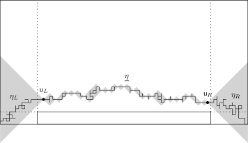
Figure 4. Decomposition of the cluster $C_{v_{L},v_{R}}$ as a concatenation $\eta_{L}\circ\underline{\eta}\circ\eta_{R}$.

By Lemma 3.6, we may restrict attention to the case when

$$({\mathsf{u}}_{L}+\underline{\eta})\cap\Delta=\varnothing.$$ (25)

In light of the above discussion, and with (23) and (24) in mind, it is natural do define the following set $\mathfrak{T}_{N}$:

Definition 4.1.

We define $\mathfrak{T}_{N}$ as the set of triples $(\eta_{L},\eta_{R},\underline{\eta})$ (see Figure 4) and the corresponding vertices (recall the definition of displacement in (5))

$${\mathsf{u}}_{L}=v_{L}+X(\eta_{L}),\quad{\mathsf{u}}_{R}=v_{R}-X(\eta_{R}),$$

in their coordinate representation (21), such that

$$v_{L}+\eta_{L}\circ\underline{\eta}\circ\eta_{R}\subset\mathbb{H}_{+}\quad\text{and, furthermore, \eqref{eq:NoInt} holds}.$$ (26)

Moreover,

$$j_{L}\in[-N,-N+2N^{\delta}+(\log N)^{2}]\quad\text{ and }\quad j_{R}\in[N-2N^{\delta}-(\log N)^{2},N],$$ (27)

and $v_{L}+\eta_{L}$ and ${\mathsf{u}}_{R}+\eta_{R}$ do not have cone-points in the interior of the vertical slabs $\mathcal{S}_{-N+2N^{\delta},j_{L}}$ and $\mathcal{S}_{j_{R},N-2N^{\delta}}$. In addition, $\max_{i}\operatorname{diam}(\eta_{i})\leq(\log N)^{2}$ and (22) holds.

Lemma 4.1.

There exist $c,C\in(0,\infty)$ such that, for all $N$ sufficiently large,

$$\Phi_{\Lambda_{+}}(v_{L}\leftrightarrow v_{R})\bigl{(}1-CN^{-c\log N}\bigr{)}\leq\sum_{(\eta_{L},\eta_{R},\underline{\eta})\in\mathfrak{T}_{N}}\Phi_{\Lambda_{+}}(\eta_{L}\circ\eta_{1}\circ\dots\circ\eta_{k}\circ\eta_{R}).$$ (28)

Now (see Section 3 in [8]), the events in the right-hand side of (28) can be represented as

$$\{\eta_{L}\circ\eta_{1}\circ\dots\circ\eta_{k}\circ\eta_{R}\}=\{v_{L}+\eta_{L}\}\cap\{{\mathsf{u}}_{L}+\underline{\eta}\}\cap\{{\mathsf{u}}_{R}+\eta_{R}\}.$$ (29)

Thus,

$$\Phi_{\Lambda_{+}}(\eta_{L}\circ\eta_{1}\circ\dots\circ\eta_{k}\circ\eta_{R})=\Phi_{\Lambda_{+}}({\mathsf{u}}_{L}+\underline{\eta}\,|\,v_{L}+\eta_{L};{\mathsf{u}}_{R}+\eta_{R})\,\Phi_{\Lambda_{+}}(v_{L}+\eta_{L};{\mathsf{u}}_{R}+\eta_{R}).$$ (30)

In view of the sharpness of phase transition proved in [14], the analysis of [8, Section 3] applies all the way up to the critical temperature. Consequently, by (3.14) of the latter paper and the restriction (25), there exists $c\in(0,\infty)$ such that

$$\exp{-{\rm e}^{-cN^{\epsilon}}}\leq\frac{\Phi_{\Lambda_{+}}({\mathsf{u}}_{L}+\underline{\eta}\,|\,v_{L}+\eta_{L};{\mathsf{u}}_{R}+\eta_{R})}{\Phi({\mathsf{u}}_{L}+\underline{\eta}\,|\,v_{L}+\eta_{L};{\mathsf{u}}_{R}+\eta_{R})}\leq\exp{{\rm e}^{-cN^{\epsilon}}}$$ (31)

for all $N$ sufficiently large, uniformly in $(\eta_{L},\eta_{R},\underline{\eta})\in\mathfrak{T}_{N}$.

Let us define the following regularized measure on $\mathfrak{T}_{N}$ or, equivalently, on the set of clusters $C_{v_{L},v_{R}}=\eta_{R}\circ\underline{\eta}\circ\eta_{R}$ with $(\eta_{L},\eta_{R},\underline{\eta})\in\mathfrak{T}_{N}$:

$$\Phi_{\Lambda_{+}}^{\mathsf{reg}}(\eta_{L}\circ\underline{\eta}\circ\eta_{R})=\frac{1}{Z_{N}}\Phi({\mathsf{u}}_{L}+\underline{\eta}\,|\,v_{L}+\eta_{L};{\mathsf{u}}_{R}+\eta_{R})\,\Phi_{\Lambda_{+}}(v_{L}+\eta_{L};{\mathsf{u}}_{R}+\eta_{R}),$$ (32)

where $Z_{N}=Z_{N}(\beta,\epsilon)$ is a normalizing constant. We have proven

Proposition 4.2.

There exists a coupling $\Psi_{N}$ between $\Phi_{\Lambda_{+}}(\,\cdot\,|\,v_{L}\longleftrightarrow v_{R})$ (viewed as a probability distribution on the set of clusters $C_{v_{L},v_{R}}$) and the probability distribution $\Phi_{\Lambda_{+}}^{\mathsf{reg}}$ on $\mathfrak{T}_{N}$ such that, for all $N$ sufficiently large,

$$\Psi_{N}\left(C_{v_{L},v_{R}}\neq\eta_{L}\circ\underline{\eta}\circ\eta_{R}\right)\leq 2CN^{-c\log N}.$$ (33)

From now on, we work only with the regularized measure $\Phi_{\Lambda_{+}}^{\mathsf{reg}}$.

4.2. Construction of the effective random walk

Recall from (18) the definition of the rectangles $\Delta=\Delta(N,\epsilon)$. Let us, first of all, define a modified set of triples $\mathfrak{T}^{*}_{N}=(\lambda_{L},\underline{\lambda},\lambda_{R})$ such that $\lambda_{L}\in\mathfrak{B}_{L},\lambda_{R}\in\mathfrak{B}_{R}$ and, in addition,

$$\underline{\lambda}=\lambda_{1}\circ\dots\circ\lambda_{M}\text{ is a concatenation of $\lambda_{i}\in\mathfrak{A}$}$$

and

$$v_{L}+\lambda_{L}\circ\underline{\lambda}\circ\lambda_{R}\subset\mathbb{H}_{+}\ \textrm{and}\ \left(v_{L}+\lambda_{L}\circ\underline{\lambda}\circ\lambda_{R}\right)\cap\Delta=\varnothing.$$

Note that irreducibility of the $\lambda_{i}$-s is not required here, since randomly glueing irreducible pieces together is necessary to recover independence in (36) [23, 26].

For $(\lambda_{L},\underline{\lambda},\lambda_{R})\in\mathfrak{T}^{*}_{N}$, set

$${\mathsf{u}}^{*}_{L}=(j^{*}_{L},u^{*}_{L})=v_{L}+X(\lambda_{L}),\ {\mathsf{u}}^{*}_{R}=(j^{*}_{R},u_{R}^{*})=v_{R}-X(\lambda_{R})={\mathsf{u}}^{*}_{L}+X(\underline{\lambda}).$$ (34)

Given two probability measures $\rho_{L,+},\rho_{R,+}$ on $\mathfrak{B}_{L}$ and $\mathfrak{B}_{R}$, respectively, and a probability measure ${\mathsf{p}}$ on $\mathfrak{A}$, one can construct the induced probability distribution $\mathsf{P}_{+}^{*}$ on $\mathfrak{T}_{N}^{*}$:

$$\mathsf{P}_{+}^{*}(\lambda_{L}\circ\underline{\lambda}\circ\lambda_{R})=\frac{1}{Z_{N}^{*}}\rho_{L}(\lambda_{L})\,\rho_{R}(\lambda_{R})\prod_{i=1}^{M}{\mathsf{p}}(\lambda_{i}).$$ (35)

The product term on the right-hand side of the last expression is interpreted as an effective random walk with i.i.d. steps distributed according to

$$\mathsf{P}(X={\mathsf{x}})=\sum_{\lambda\in\mathfrak{A}}{\mathsf{p}}(\lambda)\mathds{1}_{\{X(\lambda)={\mathsf{x}}\}}.$$ (36)

As in the case of Theorem 2.1, the following statement may be imported from [26] and from entropic repulsion estimates for random walks.

Theorem 4.3.

Let ${\mathbf{p}}$ be the (infinite-volume) probability measure on $\mathfrak{A}$ as it appears in Theorem 2.1. There exist $C\geq 0,c>0$ such that, for any $N$ large enough, one can construct two probability measures $\rho_{L,+}$ and $\rho_{R,+}$ on $\mathfrak{B}_{L}$ and $\mathfrak{B}_{R}$, respectively, such that

$$\max\bigl{\{}\rho_{L,+}\bigl{(}\theta(\lambda_{L})\notin[2N^{\delta},2N^{\delta}+\ell]\bigr{)},\rho_{R,+}\bigl{(}\theta(\lambda_{R})\notin[2N^{\delta},2N^{\delta}+\ell]\bigr{)}\bigr{\}}\leq Ce^{-c\ell}.$$ (37)

Furthermore, there exists a coupling $\Psi^{*}_{N}$ between $\mathsf{P}_{+}^{*}$ and $\Phi_{\Lambda_{+}}^{\mathsf{reg}}$ such that

$$\Psi_{N}^{*}(\eta_{L}\circ\underline{\eta}\circ\eta_{R}\neq\lambda_{R}\circ\underline{\lambda}\circ\lambda_{R})\leq CN^{-c\log N}.$$ (38)

4.3. Surface tension, geometry of Wulff shape and diffusivity constant of the effective random walk

We follow the conventions for notation introduced in Subsection 1.4. It will be convenient to write down explicit relations between the diffusivity constant of the effective random walk with i.i.d. steps $X=(\theta,\zeta)\in\mathcal{Y}^{\blacktriangleleft}$, the surface tension $\tau_{\beta^{*}}$ of the underlying Potts model and the curvature $\chi$ at $(\tau,0)\in\partial\mathbf{K}_{\beta^{*}}$, the boundary of the corresponding Wulff shape ${\mathbf{K}}_{\beta^{*}}$.

We know that $X$ has exponential moments in a neighborhood of the origin. Define

$$\mathbf{G}(r,h)=\mathsf{E}\bigl{(}{\rm e}^{-r\theta+h\zeta}\bigr{)}.$$

Then (see, e.g., Theorem 3.2 in [22]), the local parametrization of the boundary $\partial\mathbf{K}_{\beta}$ in a small neighborhood of $(\tau_{\beta},0)$ can be recorded as follows:

$$(\tau_{\beta}-r,h)\in\partial\mathbf{K}_{\beta^{*}}\iff\mathbf{G}(r,h)=1.$$ (39)

In view of lattice symmetries, a second-order expansion immediately yields the following formula for the curvature $\chi$:

$$\chi=\frac{\operatorname{\mathsf{Var}}({\zeta})}{\mathsf{E}(\theta)},$$ (40)

which coincides with the expression (44) for the diffusivity constant of the effective random walk.

4.4. Proof of Theorem 1.1

In view of Proposition 4.2 and Theorem 4.3, it suffices to prove the invariance principle for the rescaling (2) of the cluster $\Gamma=\lambda_{L}\circ\underline{\lambda}\circ\lambda_{R}$ under $\mathsf{P}_{+}^{*}$. Following (55), let us define

$$\hat{\mathfrak{e}}_{N}=\hat{\mathfrak{e}}_{N}(\lambda_{L}\circ\underline{\lambda}\circ\lambda_{R})=\mathfrak{I}_{N}\Bigl{(}v_{L},{\mathsf{u}}^{*}_{L},{\mathsf{u}}^{*}_{L}+X(\lambda_{1}),\dots,{\mathsf{u}}^{*}_{L}+\sum_{i=1}^{M}X(\lambda_{i})={\mathsf{u}}^{*}_{R},v_{R}\Bigr{)}.$$ (41)

By Proposition 4.2 and Theorem 4.3, we may restrict attention to the case when the rescaled upper and lower envelopes $\Gamma^{\pm}$ defined in (3) are close to $\hat{\mathfrak{e}}_{N}$ in the Hausdorff distance ${\rm d}_{\rm H}$ on $\mathbb{R}^{2}$,

$${\rm d}_{\text{H}}(\Gamma^{\pm},\hat{\mathfrak{e}}_{N})\leq\frac{(\log N)^{2}}{\sqrt{N}},$$ (42)

which already implies (3). Therefore, it is enough to prove an invariance principle for $\hat{\mathfrak{e}}_{N}$ under $\mathsf{P}^{*}_{+}$. This, however, readily follows from Theorem 5.3 applied to the rescaling of middle pieces $\underline{\lambda}$ and our choice of $\delta=8\epsilon<1/2$, which ensures that the rescaled boundary pieces $\lambda_{L}$ and $\lambda_{R}$ do not play a role.

4.5. Proofs of Theorems 1.2 and 1.3

Theorem 1.2 is proved by the same argument as Theorem 1.1 (remember Remark 3.1). Theorem 1.3 needs mostly the following adaptation: Lemma 3.1 will give a penalty whenever a cone-point is created on $\mathcal{L}$ and not on the whole lower space. The same strategy used in the proof then shows that the cluster avoids the symmetrized version of $\Delta(N,\epsilon)$ (see (18) in Section 3) with probability tending to one as $N\to\infty$. Conditioning on the half-space containing the maximum of $\Gamma^{+}$, one can then carry on the rest of the analysis and obtain Theorem 1.3.

5. Fluctuation theory of the effective random walk

5.1. Effective random walk

Theorem 2.1 and, subsequently, Theorem 4.3 set up the stage for considering effective random walks $\mathsf{S}$ with $\mathbb{N}\times\mathbb{Z}$-valued i.i.d. steps $X_{1},X_{2},\dots$, whose coordinates will be denoted as $X=(\theta,\zeta)$, and which have the following set of properties:

1. They have exponential tails: There exists $\alpha>0$ such that $\mathbb{E}({\rm e}^{\alpha(\theta+\absolutevalue{\zeta})})<\infty$.

2. The conditional distribution ${\mathbf{P}}(\cdot\,|\,\theta)$ of $\zeta$ is ${\mathbf{P}}$-a.s. symmetric, in particular $\theta$ and $\zeta$ are uncorrelated.

By Theorem 4.3, the displacements (recall (5)) along diamond-confined clusters $\gamma\in\mathfrak{A}$ under ${\mathsf{p}}$, that is,

$${\mathbf{P}}(X_{i}=x)={\mathsf{p}}\left(\gamma\in\mathfrak{A}\leavevmode\nobreak\ :\leavevmode\nobreak\ X(\gamma)=x\right),$$ (43)

satisfy the above assumptions.

Define the diffusivity constant (compare with (40))

$$\chi=\frac{\mathbf{Var}({\zeta})}{\mathbf{E}(\theta)}.$$ (44)

For ${\mathsf{u}}=(k,u)$, we use ${\mathbf{P}}_{\mathsf{u}}$ for the random walk $\mathsf{S}$ which starts at ${\mathsf{u}}$; $\mathsf{S}_{0}={\mathsf{u}}$. Under ${\mathbf{P}}_{\mathsf{u}}$, the position $\mathsf{S}_{i}$ of the walk after $i$ steps is given by

$$\mathsf{S}_{i}={\mathsf{u}}+\sum_{\ell=1}^{i}X_{\ell}={\mathsf{u}}+\left(\mathsf{T}_{i},\mathsf{Z}_{i}\right),\ \text{where $\mathsf{T}_{i}=\sum_{1}^{i}\theta_{\ell}$ and $\mathsf{Z}_{i}=\sum_{1}^{i}\zeta_{\ell}$}.$$ (45)

Given a subset $A\subseteq\mathbb{N}\times\mathbb{Z}$, or more generally $A\subset\mathbb{R}^{2}$, define the hitting times

$$H_{A}=\inf\left\{i\leavevmode\nobreak\ :\leavevmode\nobreak\ \mathsf{S}_{i}\in A\right\}\ \text{and write $H_{v}=H_{\left\{v\right\}}$ for vertices.}$$

Furthermore, given a subset $A\subseteq\mathbb{N}\times\mathbb{Z}$ and a stopping time $H$ write

$$\mathcal{L}_{A}(H)=\#\left\{i\leq H\leavevmode\nobreak\ :\leavevmode\nobreak\ \mathsf{S}_{i}\in A\right\}.$$

for the local time of $\mathsf{S}$ at $A$ during the time interval $[0,H]$.

5.2. Uniform repulsion estimates

We start with some general considerations and notation: Let $U_{n}$ be a zero mean one-dimensional random walk with i.i.d. increments $\xi_{k}$. A function $h$ is called harmonic for $U_{n}$ killed at leaving the positive half-line if it solves the equation

$$h(x)=\mathbf{E}[h(x+\xi_{1});x+\xi_{1}>0],\quad x\geq 0.$$

According to Doney [13], every positive solution to this equation is a multiple of the renewal function based on ascending ladder heights. If one assumes that the increments $\xi_{k}$ have finite variance then ladder heights have finite expectations. Therefore, by the standard renewal theorem, the corresponding renewal function is asymptotically linear. As a result,

$$h(x)\sim Cx\quad\text{as }x\to\infty.$$

In what follows, we will choose harmonic functions for which the latter relation holds with $C=1$. For this choice of the constant one has the representation

$$h(x)=x-\mathbf{E}_{x}[U_{\tau}],$$

where, with a slight abuse of notation we used $\mathbf{E}_{x}$ for the expectation with respect to the one-dimensional random walk $U_{n}$, which starts at $x\in\mathbb{Z}$, and where

$$\tau=\inf\{n\geq 1:U_{n}\leq 0\}.$$

Furthermore, $\mathbf{E}_{x}[U_{\tau}]$ converges, as $x\to\infty$, to a constant.

Let us go back to our $\mathbb{N}\times\mathbb{Z}$-valued effective random walks $\mathsf{S}$ as described in Subsection 5.1. Set $\mathbb{H}_{-}$ to be the lower half-plane,

$$\mathbb{H}_{-}=\left\{x=(x_{1},x_{2})\leavevmode\nobreak\ :\leavevmode\nobreak\ x_{2}<0\right\}.$$ (46)

First of all, the following asymptotic formula holds:

Theorem 5.1.

There exists a constant $C\in\mathbb{R}_{+}$ such that, as $n\to\infty$,

$$\mathbf{P}_{(0,u)}\left(H_{(n,v)}<H_{\mathbb{H}_{-}}<\infty\right)\sim C\frac{h^{+}(u)h^{-}(v)}{n^{3/2}}$$ (47)

uniformly in $u,v\in(0,\delta_{n}\sqrt{n})\cap\mathbb{N}$, where $\delta_{n}\to 0$ arbitrarily slowly, and $h^{\pm}$ are positive harmonic functions for random walks $\pm\mathsf{Z}_{n}$ killed when leaving the positive half-line.

Furthermore, there exists a constant $C$ such that

$$\mathbf{P}_{(0,u)}\left(H_{(n,v)}<H_{\mathbb{H}_{-}}<\infty\right)\sim C\frac{h^{+}(u)ve^{-v^{2}/2n\bf{Var}(\zeta)}}{n^{3/2}}$$ (48)

uniformly in $u\in(0,\delta_{n}\sqrt{n})\cap\mathbb{N}$ and $v\in(\delta_{n}\sqrt{n},\sqrt{n})\cap\mathbb{N}$.

Finally, if $\delta_{n}\to 0$ sufficiently slowly, then there exists a positive bounded function $\psi$ such that

$$\mathbf{P}_{(0,u)}\left(H_{(n,v)}<H_{\mathbb{H}_{-}}<\infty\right)\sim\frac{\psi(u/\sqrt{n},v/\sqrt{n})}{n^{1/2}}$$ (49)

uniformly in $u,v\in(\delta_{n}\sqrt{n},\sqrt{n})\cap\mathbb{N}$.

Note that, since the $\mathsf{Z}$-component of $\mathsf{S}$ is symmetric, $\mathbf{P}_{(0,u)}(H_{\mathbb{H}_{-}}<\infty)=1$ for any $u\in\mathbb{N}$, and hence the events $\{H_{\mathbb{H}_{-}}<\infty\}$ in (47)–(49) are redundant. The statement of Lemma 3.2 relies on the following fact, which is an analog of (47) for soft-core potentials:

Theorem 5.2.

For any $\delta<1$, there exists a constant $C$ such that

$${\mathbf{E}}_{(0,u)}\bigl{(}\mathds{1}_{\{H_{(n,v)}<\infty\}}\delta^{\mathcal{L}_{\mathbb{H}_{-}}(H_{(n,v)})}\bigr{)}\leq\frac{Cuv}{n^{3/2}},$$ (50)

uniformly in $n$ and in $u,v\in(0,\sqrt{n})\cap\mathbb{N}$.

5.3. Proof of Lemma 3.2

First, use (11) and the fact that edges which are incident to cone-points are necessarily pivotal, to obtain

$$\Phi_{\Lambda_{+}}({\mathsf{u}}\leftrightarrow{\mathsf{v}})\leq\Phi\Bigl{(}\mathds{1}_{\{{\mathsf{u}}\leftrightarrow{\mathsf{v}}\}}(1-\epsilon)^{|\textnormal{CPts}(C_{{\mathsf{u}},{\mathsf{v}}})\cap\Lambda_{-}|}\Bigr{)}.$$ (51)

We proceed by deriving an upper bound on the right-hand side of (51), as a direct consequence of Theorem 2.1 and of the random-walk estimate (50) of Theorem 5.2. Let us denote ${\mathsf{u}}=(k,u)$ and ${\mathsf{v}}=(k+m,v)$ with $0\leq u,v\leq\sqrt{m}$. Then, ${\mathsf{v}}\in{\mathsf{u}}+\mathcal{Y}^{\blacktriangleleft}_{\delta}$ for all $m$ large and Theorem 2.1 indeed applies, including the exponential bounds (6). In particular, as far as the derivation of (13) is concerned, we may restrict attention to boundary pieces $\gamma_{L},\gamma_{R}$ satisfying $\|X(\gamma_{L})\|,\|X(\gamma_{L})\|\leq\left(\log m\right)^{2}$. Similarly, we may restrict attention to the case when the cluster $C_{{\mathsf{u}},{\mathsf{v}}}$ does not go below $-N$.

Let $\mathsf{S}$ be the random walk with step distribution ${\mathbf{p}}$ defined in Theorem 2.1. Due to the discussion in the preceding paragraph, we need to derive an upper bound on the restricted sum which can be recorded in the language employed in Subsection 5.2 as

$$\sum_{\|{\mathsf{x}}\|,\|{\mathsf{y}}\|\leq(\log m)^{2}}\rho_{L}\left(X={\mathsf{x}}\right)\rho_{R}(X={\mathsf{y}}){\mathbf{E}}_{{\mathsf{u}}+{\mathsf{x}}}\bigl{(}\mathds{1}_{\{H_{{\mathsf{v}}-{\mathsf{y}}}<\infty\}}\delta^{\mathcal{L}_{\mathbb{H}_{-}}(H_{{\mathsf{v}}-{\mathsf{y}}})}\bigr{)}.$$ (52)

Set ${\mathsf{w}}={\mathsf{u}}+{\mathsf{x}}=(j,w)$ and ${\mathsf{z}}={\mathsf{v}}-{\mathsf{y}}=(j+n,z)$. By construction, $n\in[m-(\log m)^{2},m]$. Applying (6) and Theorem 5.2 (with a straightforward adjustment to treat the cases of $w,z\leq 0$ ), we recover the right-hand side of (13).∎

5.4. Proof of Lemma 3.4

We only sketch the proof, as it is a straightforward adaptation of the arguments in [27, Section 2.5].

Using Lemma 3.3 and the (full-space) Ornstein–Zernike asymptotics of [8], we obtain

$$\Phi_{\Lambda_{+}}(v_{L}\leftrightarrow v_{R}) \geq\Phi\bigl{(}C_{v_{L}}\subset\Lambda_{+},\,v_{L}\leftrightarrow v_{R}\bigr{)}$$

$$=\Phi\bigl{(}C_{v_{L}}\subset\Lambda_{+}\,|\,v_{L}\leftrightarrow v_{R}\bigr{)}\Phi\bigl{(}v_{L}\leftrightarrow v_{R}\bigr{)}$$

$$=\frac{C}{\sqrt{N}}e^{-2\tau N}\Phi\bigl{(}C_{v_{L}}\subset\Lambda_{+}\,|\,v_{L}\leftrightarrow v_{R}\bigr{)}.$$

We bound the probability in the right-hand side by restricting to a particular class of paths. Namely, those that connect $v_{L}$ to the vertex $\mathsf{a}=(-N+T,N+T)$ by a path going first vertically to $(-N,T)$ and then horizontally to $\mathsf{a}$, and connect $v_{R}$ to $\mathsf{b}=(N-T,N+T)$ in a symmetric way (here $T$ is a fixed large positive number). Arguing as in [27, Lemma 2.6], we then deduce that

$$\Phi\bigl{(}C_{v_{L}}\subset\Lambda_{+}\,|\,v_{L}\leftrightarrow v_{R}\bigr{)}\\ \geq C\,{\mathbf{P}}_{\mathsf{a}}(H_{\mathbb{H}_{-}}>H_{\mathsf{b}}\,|\,\infty>H_{\mathsf{b}})\,{\mathbf{P}}_{\mathsf{a}}(\mathsf{S}_{k}>\theta_{k}\;\forall k\leq H_{\mathsf{b}}\,|\,\infty>H_{\mathbb{H}_{-}}>H_{\mathsf{b}}).$$

The first probability in the right-hand side can be bounded below by $C/N$ using (47) and the local CLT. The reason for the presence of the second probability is that a sufficient condition for the cluster not to visit $\mathbb{H}_{-}$ is that the diamonds associated to the effective random walk do not intersect $\mathbb{H}_{-}$. This probability can be shown to be bounded below by a positive constant using the same argument as in [27, Lemma 2.7].

5.5. Invariance principle

Recall (44). Consider the conditional distribution of the excursion $\mathsf{S}[0,H_{(n,v)}]$ under

$$\mathbf{P}_{(0,u)}(\,\cdot\,|\,H_{(n,v)}<H_{\mathbb{H}_{-}}).$$ (53)

Fix $\epsilon>0$ small. In view of Lemma 3.6, we need to derive an invariance principle for Brownian excursion, as $n\to\infty$, uniformly in $u,v\in(n^{\epsilon},n^{5\epsilon})$. Namely, let us use $\mathbf{Q}^{n}_{u,v}$ for the law of the diffusively rescaled linear interpolation $\mathfrak{e}_{n}$ of the random-walk trajectory $\mathsf{S}[0,H_{(n,v)}]$;

$$\mathfrak{e}_{n}=\mathfrak{I}_{n}\bigl{(}\mathsf{S}[0,H_{(n,v)}]\bigr{)},$$ (54)

where, given a subset $\{(t_{1},z_{1}),(t_{2},z_{2}),\dots,(t_{k},z_{k})\}$ with $t_{1}<t_{2}<\dots<t_{k}$, $\mathfrak{I}_{n}$ is the linear interpolation through the vertices of the rescaled set

$$\Bigl{(}\frac{1}{n}t_{1},\frac{1}{\sqrt{\chi n}}z_{1}\Bigr{)},\Bigl{(}\frac{1}{n}t_{2},\frac{1}{\sqrt{\chi n}}z_{2}\Bigr{)},\dots,\Bigl{(}\frac{1}{n}t_{k},\frac{1}{\sqrt{\chi n}}z_{k}\Bigr{)}.$$ (55)

Theorem 5.3.

Let $\mathbf{Q}^{\infty}$ be the law of the positive normalized Brownian excursion $\mathfrak{e}$ on the unit interval $[0,1]$. Let $\delta_{n}\to 0$ arbitrarily slowly as $n\to\infty$ and let $u,v\in(0,\delta_{n}\sqrt{n})\cap\mathbb{N}$. Then, the limit as $n\to\infty$ of the family of distributions $\{\mathbf{Q}^{n}_{u,v}\}_{u,v\in(0,\delta_{n}\sqrt{n})\cap\mathbb{N}}$ is equal to $\mathbf{Q}^{\infty}$. More precisely,

1. The family $\{\mathbf{Q}^{n}_{u,v}\}_{u,v\in(0,\delta_{n}\sqrt{n})\cap\mathbb{N}}$ is tight.

2. For any $k$, any $0<t_{1}<t_{2}<\dots<t_{k}<1$ and any fixed bounded continuous function $F$ on $\mathbb{R}_{+}^{k}$,

   $$\lim_{n\to\infty}\mathbf{Q}^{n}_{u_{n},v_{n}}\bigl{(}F(\mathfrak{e}_{n}(t_{1}),\dots,\mathfrak{e}_{n}(t_{k}))\bigr{)}=\mathbf{Q}^{\infty}\bigl{(}F(\mathfrak{e}(t_{1}),\dots,\mathfrak{e}(t_{k}))\bigr{)},$$ (56)

   uniformly in the collections of sequences $\bigl{\{}u_{n},v_{n}\in(0,\delta_{n}\sqrt{n})\cap\mathbb{N}\bigr{\}}$.

5.6. Proofs

Proof of Theorem 5.1.

First, by the total probability formula,

$$\mathbf{P}_{(0,u)}\left(H_{\mathbb{H}_{-}}>H_{(n,v)}\in(0,\infty)\right) =\sum_{k=1}^{\infty}\mathbf{P}_{(0,u)}\left(H_{\mathbb{H}_{-}}>H_{(n,v)}=k\right)$$

$$=\sum_{k=1}^{\infty}\mathbf{P}_{(0,u)}\left(\mathsf{S}_{k}=(n,v),H_{\mathbb{H}_{-}}>k\right).$$

Fix some $\varepsilon>0$. Since $\theta$ has finite exponential moments, the exponential Chebyshev inequality implies that

$$\sum_{k<(1/\mathbf{E}\theta-\varepsilon)n}\mathbf{P}_{(0,u)}\left(\mathsf{S}_{k}=(n,v),H_{\mathbb{H}_{-}}>k\right)\leq\sum_{k<(1/\mathbf{E}\theta-\varepsilon)n}\mathbf{P}\Bigl{(}\sum_{\ell=1}^{k}\theta_{\ell}\geq n\Bigr{)}=\mathsf{O}(e^{-c\varepsilon n}).$$

Furthermore, by the same argument for lower tails, we have

$$\sum_{k>(1/\mathbf{E}\theta+\varepsilon)n}\mathbf{P}_{(0,u)}\left(\mathsf{S}_{k}=(n,v),H_{\mathbb{H}_{-}}>k\right)\leq\sum_{k>(1/\mathbf{E}\theta+\varepsilon)n}\mathbf{P}\Bigl{(}\sum_{\ell=1}^{k}\theta_{\ell}\leq n\Bigr{)}=\mathsf{O}(e^{-c\varepsilon n}).$$

Fix also a large constant $A$. Our next purpose is to estimate the probability $\mathbf{P}_{(0,u)}\left(\mathsf{S}_{k}=(n,v),H_{\mathbb{H}_{-}}>k\right)$ for $k\in[(1/\mathbf{E}\theta-\varepsilon)n,n/\mathbf{E}\theta-A\sqrt{n}]$. The main idea is to perform an exponential change of measure:

$$\mathbf{P}^{(h)}(\theta=j,\zeta=x)=\frac{e^{hj}}{\mathbf{E}e^{h\theta}}\mathbf{P}(\theta=j,\zeta=x).$$

Then, clearly,

$$\mathbf{P}_{(0,u)}\left(\mathsf{S}_{k}=(n,v),H_{\mathbb{H}_{-}}>k\right)=e^{-hn}\left(\mathbf{E}e^{h\theta}\right)^{k}\mathbf{P}^{(h)}_{(0,u)}\left(\mathsf{S}_{k}=(n,v),H_{\mathbb{H}_{-}}>k\right).$$

For all $h$ small enough, we have

$$\mathbf{E}e^{h\theta}\leq e^{h\mathbf{E}\theta+h^{2}\mathbf{Var}(\theta)}.$$

Then, choosing

$$h_{k,n}=\frac{n-k\mathbf{E}\theta}{2k\mathbf{Var}(\theta)},$$

we arrive at the upper bound

$$\mathbf{P}_{(0,u)}\left(\mathsf{S}_{k}=(n,v),H_{\mathbb{H}_{-}}>k\right)\leq\exp\left\{-\frac{(n-k\mathbf{E}\theta)^{2}}{4k\mathbf{Var}(\theta)}\right\}\mathbf{P}^{(h_{k,n})}_{(0,u)}\left(\mathsf{S}_{k}=(n,v),H_{\mathbb{H}_{-}}>k\right).$$ (57)

Define

$$\mathsf{S}_{j}^{0}=\mathsf{S}_{j}-j(0,\mathbf{E}^{(h_{k,n})}\zeta).$$

Then

$$\Bigl{\{}\mathsf{S}_{k}=(n,v),H_{\mathbb{H}_{-}}>k\Bigr{\}}$$

$$=\Bigl{\{}u+\sum_{\ell=1}^{j}\zeta_{\ell}>0\text{ for all }j\leq k,(0,u)+\mathsf{S}_{k}=(n,v)\Bigr{\}}$$

$$=\Bigl{\{}u+\sum_{\ell=1}^{j}\zeta_{\ell}^{0}>-j\mathbf{E}^{(h_{k,n})}\zeta\text{ for all }j\leq k,(0,u)+\mathsf{S}_{k}^{0}=(n,v-n\mathbf{E}^{(h_{k,n})}\zeta)\Bigr{\}}$$

$$\subseteq\Bigl{\{}u^{0}+\sum_{\ell=1}^{j}\zeta_{\ell}^{0}>0\text{ for all }j\leq k,(0,u^{0})+\mathsf{S}_{k}^{0}=(n,v^{0})\Bigr{\}},$$

where

$$u^{0}=u+n\big{|}\mathbf{E}^{(h_{k,n})}\zeta\big{|}\text{ and }v^{0}=v+n\big{|}\mathbf{E}^{(h_{k,n})}\zeta\big{|}-n\mathbf{E}^{(h_{k,n})}\zeta.$$

In other words,

$$\mathbf{P}^{(h_{k,n})}_{(0,u)}\left(\mathsf{S}_{k}=(n,v),H_{\mathbb{H}_{-}}>k\right)\leq\mathbf{P}^{(h_{k,n})}_{(0,u^{0})}\left(\mathsf{S}_{k}^{0}=(n,{v^{0}}),H^{0}_{\mathbb{H}_{-}}>k\right),$$

where $H^{0}_{\mathbb{H}_{-}}$ is the first hitting time of $\mathbb{H}_{-}$ by the modified random walk $\mathsf{S}^{0}=\left(\mathsf{T}^{0},\mathsf{Z}^{0}\right)$. Since $H^{0}_{\mathbb{H}_{-}}$ is an exit time for a one-dimensional random walk $\mathbf{Z}^{0}$ with zero mean and finite variance, one has the bound (see [2, Lemma 2.1])

$$\mathbf{P}^{(h_{k,n})}_{(0,z)}\left(H^{0}_{\mathbb{H}_{-}}>k\right)\leq c_{1}\frac{z+1}{\sqrt{k}}$$

uniformly in all $z>0$.

Using this bound in the proof of [10, Lemma 28], one gets easily the bound

$$\mathbf{P}^{(h_{k,n})}_{(0,u^{0})}\left(\mathsf{S}_{k}^{0}=(n,{v^{0}}),H^{0}_{\mathbb{H}_{-}}>k\right)\leq c_{2}\frac{(u^{0}+1)(v^{0}+1)}{k^{2}}$$

uniformly in all positive $u^{0},v^{0}$.

Recall that $\theta$ and $\zeta$ are uncorrelated. Then, by the Taylor formula,

$$\mathbf{E}^{(h)}\zeta=\frac{\mathbf{E}(\zeta e^{h\theta})}{\mathbf{E}e^{h\theta}}=\frac{h^{2}}{2}\mathbf{E}(\theta^{2}\zeta)+{\mathsf{o}}(h^{2}),\quad h\to 0.$$

Therefore, for small $h_{k,n}$,

$$\absolutevalue{\mathbf{E}^{(h_{k,n})}\zeta}\leq ah^{2}_{k,n}\quad\text{with}\ a=\mathbf{E}|\theta^{2}\zeta|.$$

As a result, we have

$$\mathbf{P}^{(h_{k,n})}_{(0,u)}\left(\mathsf{S}_{k}=(n,v),H_{\mathbb{H}_{-}}>k\right)\leq c_{3}\frac{(u+nh^{2}_{k,n})(v+nh^{2}_{k,n})}{k^{2}}.$$

Combining this bound with (57), summing over $k$ and using the fact that the functions $h^{\pm}$ are asymptotically linear, we obtain

$$\sum_{k\in[(1/\mathbf{E}\theta-\varepsilon)n,n/\mathbf{E}\theta-A\sqrt{n}]}\mathbf{P}_{(0,u)}\left(\mathsf{S}_{k}=(n,v),H_{\mathbb{H}_{-}}>k\right)\leq\frac{f_{1}(A)h^{+}(u)h^{-}(v)}{n^{3/2}},$$ (58)

where $f_{1}(A)\to 0$ as $A\to\infty$. This estimate is uniform in $u,v\in(0,\sqrt{n})\cap\mathbb{N}$.,

The same argument gives, also uniformly in $u,v\in(0,\sqrt{n})\cap\mathbb{N}$,

$$\sum_{k\in[n/\mathbf{E}\theta+A\sqrt{n},(1/\mathbf{E}\theta+\varepsilon)n]}\mathbf{P}_{(0,u)}\left(\mathsf{S}_{k}=(n,v),H_{\mathbb{H}_{-}}>k\right)\leq\frac{f_{2}(A)h^{+}(u)h^{-}(v)}{n^{3/2}},$$ (59)

where $f_{2}(A)\to 0$ as $A\to\infty$.

For $k\in[n/\mathbf{E}\theta-A\sqrt{n},n/\mathbf{E}\theta+A\sqrt{n}]$ one can repeat the proof of the local limit theorems from [10]. Compared to that paper, we have a rather particular case: a two-dimensional random walk confined to the upper half-plane. But we want to get a result which is valid not only for bounded start- and endpoints. Since we have a walk in the upper half-plane, the corresponding harmonic function depends on the second coordinate only and is equal to the harmonic function of the walk $Z_{n}$ killed at leaving $(0,\infty)$. So, we only have to show that the convergence in [10, Lemma 21] holds for all starting points $(0,u)$ with $u\leq\delta_{n}\sqrt{n}$. More precisely, we need to prove that

$$\mathbf{E}_{(0,u)}[Z_{\nu_{k}};H_{\mathbb{H}_{-}}>\nu_{k},\nu_{k}\leq k^{1-\varepsilon}]=h^{+}(u)(1+{\mathsf{o}}(1))$$ (60)

uniformly in $u\leq\delta_{n}\sqrt{n}$ and $k\in[n/\mathbf{E}\theta-A\sqrt{n},n/\mathbf{E}\theta+A\sqrt{n}]$. Above, $\nu_{k}$ is the first hitting time of the positive half-space $(k^{1/2-\epsilon},0)+\mathbb{H}_{+}$. The relation (60) leads to the fact that all the arguments in [10, Sections 4 and 5] hold uniformly in $u\in(0,\delta_{n}\sqrt{n})$. Then, repeating the proof in [10, Theorem 6], we obtain

$$\mathbf{P}_{(0,u)}\left(\mathsf{S}_{k}=(n,v),H_{\mathbb{H}_{-}}>k\right)\sim c_{4}\frac{h^{+}(u)h^{-}(v)}{k^{2}}\exp\left\{-\frac{(n-k\mathbf{E}\theta)^{2}}{2k\mathbf{Var}(\theta)}\right\},$$

uniformly in $u,v\in(0,\delta_{n}\sqrt{n})\cap\mathbb{N}$. Summing over $k$, we get

$$\sum_{k\in[n/\mathbf{E}\theta-A\sqrt{n},n/\mathbf{E}\theta+A\sqrt{n}]}\mathbf{P}_{(0,u)}\left(\mathsf{S}_{k}=(n,v),H_{\mathbb{H}_{-}}>k\right)\sim(C_{5}-f_{3}(A))\frac{h^{+}(u)h^{-}(v)}{n^{3/2}},$$ (61)

where $f_{3}(A)\to 0$ as $A\to\infty$.

Combining all the estimates above, we finally deduce the asymptotic relation (47). Thus, it remains to prove (60). Here one can use again the fact that we are dealing with a one-dimensional random walk. Since $Z_{n}$ is a martingale, we use the optional stopping theorem to obtain

$$u=\mathbf{E}_{(0,u)}Z_{\nu_{k}\wedge H_{\mathbb{H}_{-}}}=\mathbf{E}_{(0,u)}[Z_{\nu_{k}};\nu_{k}<H_{\mathbb{H}_{-}}]+\mathbf{E}_{(0,u)}[Z_{H_{\mathbb{H}_{-}}};\nu_{k}\geq H_{\mathbb{H}_{-}}].$$

Consequently,

$$\mathbf{E}_{(0,u)}[Z_{\nu_{k}};\nu_{k}<H_{\mathbb{H}_{-}},\nu_{k}\leq k^{1-\epsilon}]\\ =u-\mathbf{E}_{(0,u)}[Z_{H_{\mathbb{H}_{-}}};\nu_{k}\geq H_{\mathbb{H}_{-}}]-\mathbf{E}_{(0,u)}[Z_{\nu_{k}};\nu_{k}<H_{\mathbb{H}_{-}},\nu_{k}>k^{1-\epsilon}].$$ (62)

Recalling that $\mathbf{E}_{(0,u)}H_{\mathbb{H}_{-}}$ is bounded and that $h^{+}(u)\sim u$ as $u\to\infty$, one gets easily

$$u-\mathbf{E}_{(0,u)}[Z_{H_{\mathbb{H}_{-}}};\nu_{k}\geq H_{\mathbb{H}_{-}}]=h^{+}(u)(1+{\mathsf{o}}(1))$$ (63)

uniformly in $u$. Furthermore, by the Cauchy–Schwarz inequality,

$$\mathbf{E}_{(0,u)}[Z_{\nu_{k}};\nu_{k}<H_{\mathbb{H}_{-}},\nu_{k}>k^{1-\epsilon}]\leq\mathbf{E}^{1/2}_{(0,u)}[Z^{2}_{\nu_{k}};\nu_{k}<H_{\mathbb{H}_{-}}]\mathbf{P}^{1/2}_{(0,u)}(\nu_{k}>k^{1-\epsilon},\nu_{k}<H_{\mathbb{H}_{-}}).$$

Obviously, $Z^{2}_{\nu_{k}}=(Z_{\nu_{k}-1}+\zeta_{\nu_{k}})^{2}\leq 2k^{1-2\varepsilon}+2\zeta_{\nu_{k}}^{2}$ on the event $\{\nu_{k}<H_{\mathbb{H}_{-}}\}$. Thus, using the total probability formula, we get

$$\mathbf{E}_{(0,u)}[Z^{2}_{\nu_{k}};\nu_{k}<H_{\mathbb{H}_{-}}]\leq 2(k^{1-2\epsilon}+\mathbf{E}\zeta)\mathbf{E}_{(0,u)}[\nu_{k}\wedge H_{\mathbb{H}_{-}}]\leq Ck^{2-4\epsilon}.$$

In the last step, we have used the bound $\mathbf{E}_{(0,u)}[\nu_{k}\wedge H_{\mathbb{H}_{-}}]\leq Ck^{1-2\epsilon}$, which follows from the normal approximation. By [10, Lemma 14],

$$\mathbf{P}_{(0,u)}(\nu_{k}>k^{1-\epsilon},\nu_{k}<H_{\mathbb{H}_{-}}) \leq\mathbf{P}_{(0,u)}(\nu_{k}>k^{1-\epsilon},H_{\mathbb{H}_{-}}>k^{1-\epsilon})\leq e^{-Ck^{\epsilon}}.$$

As a result,

$$\mathbf{E}_{(0,u)}[Z_{\nu_{k}};\nu_{k}<H_{\mathbb{H}_{-}},\nu_{k}>k^{1-\epsilon}]=\mathsf{O}(e^{-Ck^{\epsilon}})$$ (64)

for some $C>0$. Combining (62)–(64), we obtain (60).

The derivations of (48) and (49) are very similar and even simpler and are thus omitted. ∎

Proof of Theorem 5.2.

Let us introduce some provisional notation:

Hitting times. $\mathbb{H}^{k}_{-}=(0,-k)+\mathbb{H}_{-}=\left\{x=(x_{1},x_{2})\leavevmode\nobreak\ :\leavevmode\nobreak\ x_{2}<-k\right\}$ for the negative half-planes passing through the shifted points $(0,-k)$.

Minimal heights. Given an in general random time $H\in\mathbb{N}$, let $\mathsf{Z}_{*}(H)=\min_{\ell=0,\dots,H}\mathsf{Z}_{\ell}$ be the minimal value of the vertical coordinate $\mathsf{Z}$ of the random-walk trajectory $\mathsf{S}[0,H]$ on the time interval $[0,H]$. Furthermore, let $m_{*}(H)=\min\{m\,:\,(m,\mathsf{Z}_{*}(H))\in\mathsf{S}[0,H]\}$ be the horizontal projection of the leftmost vertex of $\mathsf{S}[0,H]$, at which the minimal height $\mathsf{Z}_{*}(H)$ was attained.

Evidently,

$${\mathbf{E}}_{(0,u)}\bigl{(}\mathds{1}_{\{H_{(n,v)}<\infty\}}\delta^{\mathcal{L}_{\mathbb{H}_{-}}(H_{(n,v)})}\bigr{)}\leq\\ {\mathbf{P}}_{(0,u)}(H_{(n,v)}<H_{\mathbb{H}_{-}})+\sum_{k=0}^{\infty}{\mathbf{E}}_{(0,u)}\bigl{(}\mathds{1}_{\{H_{(n,v)}<\infty\}}\mathds{1}_{\{Z^{*}(H_{(n,v)})=-k\}}\delta^{\mathcal{L}_{\mathbb{H}_{-}}(H_{(n,v)})}\bigr{)}.$$ (65)

The first term on the right-hand side above is controlled by Theorem 5.1. In view of the exponential tails, we may fix $\epsilon>0$ small and restrict attention to such terms in the above sum, which satisfy $k\leq n^{1/2+\epsilon}$.

Now,

$${\mathbf{E}}_{(0,u)}\bigl{(}\mathds{1}_{\{H_{(n,v)}<\infty\}} \mathds{1}_{\{Z^{*}(H_{(n,v)})=-k\}}\delta^{\mathcal{L}_{\mathbb{H}_{-}}(H_{(n,v)})}\bigr{)}$$ (66)

$$={\mathbf{E}}_{(0,u)}\bigl{(}\mathds{1}_{\{m_{*}\in[0,n/2]\}}\mathds{1}_{\{H_{(n,v)}<\infty\}}\mathds{1}_{\{Z^{*}(H_{(n,v)})=-k\}}\delta^{\mathcal{L}_{\mathbb{H}_{-}}(H_{(n,v)})}\bigr{)}$$

$$+{\mathbf{E}}_{(0,u)}\bigl{(}\mathds{1}_{\{m_{*}\in[n/2,n]\}}\mathds{1}_{\{H_{(n,v)}<\infty\}}\mathds{1}_{\{Z^{*}(H_{(n,v)})=-k\}}\delta^{\mathcal{L}_{\mathbb{H}_{-}}(H_{(n,v)})}\bigr{)}.$$

We shall consider only the first term on the right-hand side above, the second one is completely similar. Let us decompose with respect to the possible values of $m_{*}$

$${\mathbf{E}}_{(0,u)}\bigl{(}\mathds{1}_{\{m_{*}\in[0,n/2]\}}\mathds{1}_{\{H_{(n,v)}<\infty\}}\mathds{1}_{\{Z^{*}(H_{(n,v)})=-k\}}\delta^{\mathcal{L}_{\mathbb{H}_{-}}(H_{(n,v)})}\bigr{)}\\ =\sum_{m=1}^{\lfloor n/2\rfloor}{\mathbf{E}}_{(0,u)}\bigl{(}\mathds{1}_{\{m_{*}=m\}}\mathds{1}_{\{H_{(n,v)}<\infty\}}\mathds{1}_{\{Z^{*}(H_{(n,v)})=-k\}}\delta^{\mathcal{L}_{\mathbb{H}_{-}}(H_{(n,v)})}\bigr{)}.$$

We shall rely on several crude upper bounds. The first one is

$${\mathbf{E}}_{(0,u)}\bigl{(}\mathds{1}_{\{m_{*}=m\}}\mathds{1}_{\{H_{(n,v)}<\infty\}}\mathds{1}_{\{Z^{*}(H_{(n,v)})=-k\}}\delta^{\mathcal{L}_{\mathbb{H}_{-}}(H_{(n,v)})}\bigr{)}$$

$$\quad\leq{\mathbf{E}}_{(0,u)}\Bigl{(}\mathds{1}_{\{H_{(m,-k)}=H_{\mathbb{H}^{k-1}_{-}}\}}{\mathbf{E}}_{(m,-k)}\bigl{(}\mathds{1}_{\{H_{(n,v)}<H_{\mathbb{H}^{k}_{-}}\}}\delta^{\mathcal{L}_{\mathbb{H}_{-}}(H_{(n,v)})}\bigr{)}\Bigr{)}$$

$$\quad\leq{{\rm e}^{-cn\wedge\frac{n^{2}}{k}}}+{\mathbf{E}}_{(0,u)}\Bigl{(}\mathds{1}_{\{H_{(m,-k)}=H_{\mathbb{H}^{k-1}_{-}}\}}{\mathbf{E}}_{(m,-k)}\bigl{(}\delta^{\mathcal{L}_{\mathbb{H}_{-}}(k)}{\mathbf{P}}_{{\mathsf{S}}_{k}}(H_{(n,v)}<H_{\mathbb{H}^{k}_{-}})\bigr{)}\Bigr{)}.$$ (67)

For $k\leq n^{1/2+\epsilon}$, the first summand in (5.6) above is negligible. We claim that there exist $c,C\in(0,\infty)$ such that

$${\mathbf{E}}_{(m,-k)}\bigl{(}\delta^{\mathcal{L}_{\mathbb{H}_{-}}(k)}{\mathbf{P}}_{{\mathsf{S}}_{k}}(H_{(n,v)}<H_{\mathbb{H}^{k}_{-}})\bigr{)}\leq C{\rm e}^{-c\sqrt{k}}{\mathbf{P}}_{(m,-k)}(H_{(n,v)}<H_{\mathbb{H}^{k}_{-}}),$$ (68)

uniformly in $n\in\mathbb{N}$ sufficiently large and, then, in $v\leq\sqrt{n}$, $m\in[0,n/2]$ and (for $\epsilon>0$ being fixed appropriately small) $k\in[0,n^{1/2+\epsilon}]$. We shall relegate the justification of (68) to the end of the proof. At this stage, note that (68) (and its analogue for the second term on the right-hand side of (66)) would imply that

$${\mathbf{E}}_{(0,u)}\bigl{(}\mathds{1}_{\{H_{(n,v)}<\infty\}}\mathds{1}_{\{Z^{*}(H_{(n,v)})=-k\}}\delta^{\mathcal{L}_{\mathbb{H}_{-}}(H_{(n,v)})}\bigr{)}\\ \leq C{\rm e}^{-c\sqrt{k}}{\mathbf{P}}_{(0,u)}\bigl{(}H_{(n,v)}<\infty;Z^{*}(H_{(n,v)})=-k\bigr{)}.$$ (69)

It follows that, as far as the sum in (65) is concerned, we may further restrict attention to $k\leq\frac{1}{c}(\log n)^{3}$. In the latter case, however, Theorem 5.1 applies and

$${\mathbf{P}}_{(0,u)}(H_{(n,v)}<H_{\mathbb{H}^{k}_{-}})\sim C\frac{(u+k)(v+k)}{n^{3/2}}.$$ (70)

Consequently,

$${\mathbf{P}}_{(0,u)}\bigl{(}H_{(n,v)}<\infty;\mathsf{Z}_{*}(H_{(n,v)})=-k\bigr{)}\\ ={\mathbf{P}}_{(0,u)}(H_{(n,v)}<H_{\mathbb{H}^{k+1}_{-}})-{\mathbf{P}}_{(0,u)}(H_{(n,v)}<H_{\mathbb{H}^{k}_{-}})\\ \leq C\frac{(u+k+1)(v+k+1)}{n^{3/2}}.$$ (71)

Substituting (69) and (71) into (65) yields: There exist $c,C\in(0,\infty)$, such that

$${\mathbf{E}}_{(0,u)}\bigl{(}\mathds{1}_{\{H_{(n,v)}<\infty\}}\mathds{1}_{\{Z^{*}(H_{(n,v)})=-k\}}\delta^{\mathcal{L}_{\mathbb{H}_{-}}(\mathsf{H}_{(n,v)})}\bigr{)}\leq\sum_{k=0}^{\infty}C\frac{(u+k)(v+k){\rm e}^{-c\sqrt{k}}}{n^{3/2}},$$ (72)

and we are home.

Proof of (68). First of all, in view of Theorem 5.1, the right-hand side of (68) satisfies

$${\mathbf{P}}_{(m,-k)}(H_{(n,v)}<H_{\mathbb{H}^{k}_{-}})\geq C\frac{(v+\min\left\{k,\sqrt{n}\right\})}{n^{3/2}},$$ (73)

uniformly in $m$ and $k$ in question. Consider now the left-hand side of (68). Since $k\leq n^{1/2+\epsilon}$ and $\epsilon$ is small, we may rely on moderate deviation estimates and restrict attention to $\absolutevalue{S_{k}-(m,-k)}=\bigl{\lvert}\sum_{1}^{k}\zeta_{i}\bigr{\rvert}\leq\sqrt{n}$. In the latter case Theorem 5.1 applies, and the following upper bound holds: There exists $C^{*}<\infty$, such that

$${\mathbf{E}}_{(m,-k)}\bigl{(}\delta^{\mathcal{L}_{\mathbb{H}_{-}}(k)}{\mathbf{P}}_{{\mathsf{S}}_{k}}({H_{(n,v)}<H_{\mathbb{H}^{k}_{-}}})\bigr{)}\leq C^{*}{\mathbf{E}}_{(m,-k)}\Bigl{(}\delta^{\mathcal{L}_{\mathbb{H}_{-}}(k)}\frac{v+\bigl{\lvert}\sum_{1}^{k}\zeta_{i}\bigr{\rvert}}{n^{3/2}}\Bigr{)}.$$ (74)

It remains to notice that, by the usual large deviation upper bounds under Cramér’s condition, there exists $c^{*}>0$ such that

$${\mathbf{E}}_{(m,-k)}\Bigl{(}\delta^{\mathcal{L}_{\mathbb{H}_{-}}(k)}\bigl{(}v+\bigl{\lvert}\sum_{1}^{k}\zeta_{i}\bigr{\rvert}\bigr{)}\Bigr{)}\leq C^{*}{\rm e}^{-c^{*}k}(v+k),$$ (75)

uniformly in $k,v\in\mathbb{Z}_{+}$. Together with (73), this implies (68). ∎

Proof of Theorem 5.3.

The above changes in the arguments from [10] allow one to repeat the proof of [15, Theorem 6], which gives the convergence of a properly centered and rescaled walk $\sf S_{n}$ towards the two-dimensional Brownian bridge conditioned to stay in the upper half-plane. This convergence is uniform in the range of $u,v$ as formulated in Theorem 5.3. In particular, we have convergence of each coordinate of the two-dimensional walk $\sf S_{n}$. More precisely, again uniformly in $u,v\in(0,\delta_{n}\sqrt{n})\cap\mathbb{N}$ and, also for each $A$ fixed, uniformly in the number of steps $k\in[n/\mathbf{E}\theta-A\sqrt{n},n/\mathbf{E}\theta+A\sqrt{n}]\cap\mathbb{N}$ which shows up in the principal sum (61),

$$\mathbf{P}_{(0,u)}\bigl{(}\max_{j\leq k}|\mathsf{T}_{j}-j\mathbf{E}\theta|>\delta k\bigm{|}\mathsf{S}_{k}=(n,v),H_{\mathbb{H}_{-}}>k\bigr{)}\to 0,$$ (76)

and, for any $\ell\in\mathbb{N}$, any $0<t_{1}<t_{2}<\dots<t_{\ell}<1$, any fixed bounded continuous function $F$ on $\mathbb{R}_{+}^{\ell}$,

$$\mathbf{E}_{(0,u)}\left[F\left(\mathfrak{z}_{k}(t_{1}),\dots,\mathfrak{z}_{k}(t_{\ell})\right)\big{|}\mathsf{S}_{k}=(n,v),H_{\mathbb{H}_{-}}>k\right]\to\mathbf{Q}^{\infty}\left[F\left(\mathfrak{z}_{k}(t_{1}),\dots,\mathfrak{z}_{k}(t_{\ell})\right)\right],$$ (77)

where $\mathfrak{z}_{k}$ is the linear interpolation with nodes

$$\Bigl{(}\frac{1}{k},\frac{{\sf Z}_{1}}{\sqrt{k\mathbf{Var}(\theta))}}\Bigr{)},\Bigl{(}\frac{2}{k},\frac{{\sf Z}_{2}}{\sqrt{k\mathbf{Var}(\theta))}}\Bigr{)},\dots,\Bigl{(}\frac{k-1}{k},\frac{{\sf Z}_{k-1}}{\sqrt{k\mathbf{Var}(\theta))}}\Bigr{)},\Bigl{(}1,\frac{v}{\sqrt{k\mathbf{Var}(\theta))}}\Bigr{)}.$$

Thus, in view of (58) and (59), it remains to bound the difference between this interpolation and the interpolation in (55) for $k$ such that $\absolutevalue{n-k\mathbf{E}\theta}\leq A\sqrt{n}$. To this end, we notice that the random change of time $h_{k}$, defined as the linear interpolation of $(\ell/k,T_{\ell}/n)$, transforms (55) into $\mathfrak{z}_{k}$. Combining this observation with (76) and (77), we obtain the convergence of (55) in the Skorokhod $J_{1}$-topology. Since the limiting process — Brownian excursion — has continuous paths, one has also the convergence in the uniform topology. This follows from Theorem 2.6.2 in Skorokhod’s classical paper [28]. ∎

Appendix A A Monotone Coupling

For $\Delta\subset E_{\mathbb{Z}^{2}}$ finite, denote $\Phi_{a,\Delta}\equiv\Phi_{a,\Delta}^{0}$ the random-cluster measure in $\Delta$ with free ($0$) boundary condition and weights $e^{\beta}-1$ on edges with both endpoints having nonnegative second coordinate and weight $a$ on the others. In particular, $\Phi_{0,\Lambda}$ is the random-cluster measure on the half-box $\Lambda_{+}$ with free boundary condition and weights $e^{\beta}-1$.

In this section, we construct a monotone coupling of $\Phi_{b,\Delta}$ and $\Phi_{a,\Delta}$ for $b>a$. The construction follows closely the one used in the proof of [19, Theorem 3.47]. We fix $\Delta$ and let $\Delta^{+}=\Delta\cap(\mathbb{R}\times\mathbb{R}_{\geq 0})$ and $\Delta^{-}=\Delta\cap(\mathbb{R}\times\mathbb{R}_{<0})$; both are seen as the graphs induced by their set of edges, where edges are identified with the corresponding open line segments. For a finite set of edges $E$, denote by $\mathrm{o}_{-}(E)$ the number of edges in $E$ with at least one endpoint having negative second coordinate.

Let $e_{1},\dots,e_{\absolutevalue{E_{\Delta}}}$ be an enumeration of the edges of $\Delta$ and set $E_{i}=\{e_{1},\dots,e_{i}\}$. Let $(U_{i})_{i=1}^{\absolutevalue{E_{\Delta}}}$ be an i.i.d. family of uniform random variables on $[0,1]$. From a realization $u=(u_{i})_{i}$ of $U=(U_{i})_{i}$, we construct two configurations $\omega=\omega(u)$ and $\eta=\eta(u)$ with joint distribution $\Psi$ as follows:

Set $i=1$

while $i\leq|E_{\Delta}|$ do

       Set $\omega_{e_{i}}=\mathds{1}_{\{u_{i}<\Phi_{b}(X_{e_{i}}=1\,|\,X_{E_{i-1}}=\omega_{E_{i-1}})\}}$

       Set $\eta_{e_{i}}=\mathds{1}_{\{u_{i}<\Phi_{a}(X_{e_{i}}=1\,|\,X_{E_{i-1}}=\eta_{E_{i-1}})\}}$

       Update $i=i+1$

      

end while

Algorithm 1 Constructing $\omega,\eta$.

Monotonicity of random-cluster measures in their parameters and boundary condition ensures that $\omega\geq\eta$. Direct computation shows that $\omega(U)\sim\Phi_{b}$ and $\eta(U)\sim\Phi_{a}$.

Claim 1.

For any $e_{M}\in\Delta^{-}$,

$$\Psi(\omega_{e_{M}}=1,\,\eta_{e_{M}}=0\,|\,U_{1}=u_{1},\dots,U_{M-1}=u_{M-1})\geq\frac{b-a}{(b+q)(b+1)}$$

uniformly over $u_{1},\dots,u_{M-1}$.

Proof.

First, notice that (denoting $\omega_{E_{M-1}}(u_{1},\dots,u_{M-1})$ the configuration $\omega$ restricted to $E_{M-1}$ and similarly for $\eta$)

$$\Psi(\omega_{e_{M}}=1,\,\eta_{e_{M}}=0 \,|\,U_{1}=u_{1},\dots,U_{M-1}=u_{M-1})$$

$$=\Phi_{b}(X_{e_{M}}=1\,|\,X_{E_{i-1}}=\omega_{E_{i-1}})-\Phi_{a}(X_{e_{M}}=1\,|\,X_{E_{i-1}}=\eta_{E_{i-1}})$$

$$\geq\Phi_{b}(X_{e_{M}}=1\,|\,X_{E_{i-1}}=\omega_{E_{i-1}})-\Phi_{a}(X_{e_{M}}=1\,|\,X_{E_{i-1}}=\omega_{E_{i-1}})$$

$$=\int_{a}^{b}\frac{\differential}{\differential s}\Phi_{s}(X_{e_{M}}=1\,|\,X_{E_{i-1}}=\omega_{E_{i-1}})\,\differential s.$$

The claim will thus follow once we establish that $\frac{\differential}{\differential s}\Phi_{s}(X_{e_{M}}=1\,|\,X_{E_{i-1}}=\omega_{E_{i-1}})\geq(b+q)^{-1}(b+1)^{-1}$ for any $s\leq b$. Write $\Phi_{s}^{*}(\cdot)=\Phi_{s}(\cdot\,|\,X_{E_{i-1}}=\omega_{E_{i-1}})$; this is a random-cluster measure on $E_{\Lambda}\setminus E_{M-1}$. Let $X\sim\Phi_{s}^{*}$. Then,

$$\frac{\differential}{\differential s}\Phi_{s}^{*}(X_{e_{M}}=1) =\frac{1}{s}\mathrm{Cov}_{s}^{*}\bigl{(}\absolutevalue{\mathrm{o}_{-}(X)},\,X_{e_{M}}\bigr{)}$$

$$=\frac{1}{s}\mathrm{Cov}_{s}^{*}\bigl{(}\absolutevalue{\mathrm{o}_{-}(X)}-X_{e_{M}},\,X_{e_{M}}\bigr{)}+\frac{1}{s}\Phi_{s}^{*}(X_{e_{M}}=1)\Phi_{s}^{*}(X_{e_{M}}=0)$$

$$\geq\frac{1}{s}\frac{s}{s+q}\frac{1}{s+1}\geq\frac{1}{(b+q)(b+1)},$$

since $\absolutevalue{\mathrm{o}_{-}(X)}-X_{e_{M}}$ is a nondecreasing function and is thus positively correlated with $X_{e_{M}}$ (the remainder follows from finite energy). ∎

As $\Psi(\omega_{e_{M}}=1\,|\,U_{1}=u_{1},\dots,U_{M-1}=u_{M-1})\leq\frac{b}{1+b}$ (by finite energy), one has

$$\Psi(\eta_{e_{M}}=0\,|\,\omega_{e_{M}}=1,\,U_{1}=u_{1},\dots,U_{M-1}=u_{M-1})\geq\frac{b-a}{(b+q)(b+1)}\frac{1+b}{b}=\frac{b-a}{(b+q)b}.$$

Write $\epsilon=\epsilon(a,b)=\frac{b-a}{(b+q)b}$. This implies that, for any configuration $\psi$ and any set $A\subset E_{\Delta^{-}}$ with $\psi_{e}=1$ for all $e\in A$,

$$\Psi(\omega=\psi,\,\eta_{e}=1\forall e\in A)\leq(1-\epsilon)^{|A|}\,\Phi_{b}(\psi).$$ (78)

Indeed, writing $D_{i}=\{\eta_{e_{i}}=1\}$ if $e_{i}\in A$ and $D_{i}=\{\eta_{e_{i}}\in\{0,1\}\}$ otherwise and setting $D_{E_{i}}=\bigcap_{j\leq i}D_{j}$, we get

$$\frac{\Psi(\omega=\psi,\,\eta_{e}=1\forall e\in A)}{\Psi(\omega=\psi)} \leq\prod_{i=1}^{\absolutevalue{E_{\Lambda}}}\frac{\Psi(\omega_{e_{i}}=\psi_{e_{i}},\,D_{i}\,|\,\omega_{E_{i-1}}=\psi_{E_{i-1}},\,D_{E_{i-1}})}{\Psi(\omega_{e_{i}}=\psi_{e_{i}}\,|\,\omega_{E_{i-1}}=\psi_{E_{i-1}})}$$

$$\leq\prod_{i:\,e_{i}\in A}\Psi(\eta_{e_{i}}=1\,|\,\omega_{e_{i}}=1,\,\omega_{E_{i-1}}=\psi_{E_{i-1}},\,D_{E_{i-1}})$$

$$\leq(1-\epsilon)^{|A|}.$$

References

- [1] D. B. Abraham and P. Reed. Phase separation in the two-dimensional Ising ferromagnet. Phys. Rev. Lett., 33:377–379, Aug 1974.
- [2] V. I. Afanasyev, J. Geiger, G. Kersting, and V. A. Vatutin. Criticality for branching processes in random environment. Ann. Probab., 33(2):645–673, 2005.
- [3] V. Beffara and H. Duminil-Copin. The self-dual point of the two-dimensional random-cluster model is critical for . Probab. Theory Related Fields, 153(3-4):511–542, 2012.
- [4] J. Bricmont, J. L. Lebowitz, and C. E. Pfister. On the local structure of the phase separation line in the two-dimensional Ising system. J. Statist. Phys., 26(2):313–332, 1981.
- [5] M. Campanino and D. Ioffe. Ornstein-Zernike theory for the Bernoulli bond percolation on . Ann. Probab., 30(2):652–682, 2002.
- [6] M. Campanino, D. Ioffe, and O. Louidor. Finite connections for supercritical Bernoulli bond percolation in 2D. Markov Process. Related Fields, 16(2):225–266, 2010.
- [7] M. Campanino, D. Ioffe, and Y. Velenik. Ornstein-Zernike theory for finite range Ising models above . Probab. Theory Related Fields, 125(3):305–349, 2003.
- [8] M. Campanino, D. Ioffe, and Y. Velenik. Fluctuation theory of connectivities for subcritical random cluster models. Ann. Probab., 36(4):1287–1321, 2008.
- [9] A. De Masi, D. Ioffe, I. Merola, and E. Presutti. Metastability and uphill diffusion. Provisional title, in preparation.
- [10] D. Denisov and V. Wachtel. Random walks in cones. The Annals of Probability, 43(3):992–1044, 2015.
- [11] R. Dobrushin. A statistical behaviour of shapes of boundaries of phases. In R. Kotecký, editor, Phase Transitions: Mathematics, Physics, Biology…, pages 60–70. 1992.
- [12] R. Dobrushin, R. Kotecký, and S. Shlosman. Wulff construction, volume 104 of Translations of Mathematical Monographs. American Mathematical Society, Providence, RI, 1992.
- [13] R. A. Doney. The martin boundary and ratio limit theorems for killed random walks. Journal of the London Mathematical Society, 58(3):761–768, 1998.
- [14] H. Duminil-Copin and I. Manolescu. The phase transitions of the planar random-cluster and potts models with are sharp. Probability Theory and Related Fields, 164(3):865–892, 2016.
- [15] J. Duraj and V. Wachtel. Invariance principles for random walks in cones. arXiv:1508.07966, 2015.
- [16] R. Durrett. On the shape of a random string. Ann. Probab., 7(6):1014–1027, 1979.
- [17] G. Gallavotti. The phase separation line in the two-dimensional Ising model. Comm. Math. Phys., 27:103–136, 1972.
- [18] L. Greenberg and D. Ioffe. On an invariance principle for phase separation lines. Ann. Inst. H. Poincaré Probab. Statist., 41(5):871–885, 2005.
- [19] G. Grimmett. The random-cluster model, volume 333 of Grundlehren der Mathematischen Wissenschaften. Springer-Verlag, Berlin, 2006.
- [20] Y. Higuchi. On some limit theorems related to the phase separation line in the two-dimensional Ising model. Z. Wahrsch. Verw. Gebiete, 50(3):287–315, 1979.
- [21] D. Ioffe. Ornstein-Zernike behaviour and analyticity of shapes for self-avoiding walks on . Markov Process. Related Fields, 4(3):323–350, 1998.
- [22] D. Ioffe. Multidimensional random polymers: a renewal approach. In Random walks, random fields, and disordered systems, volume 2144 of Lecture Notes in Math., pages 147–210. Springer, Cham, 2015.
- [23] D. Ioffe, S. Ott, Shlosman S., and Y. Velenik. Critical prewetting in the 2d Ising model. In preparation.
- [24] D. Ioffe, S. Shlosman, and F. L. Toninelli. Interaction versus entropic repulsion for low temperature Ising polymers. J. Stat. Phys., 158(5):1007–1050, 2015.
- [25] S. Miracle-Sole. Surface tension, step free energy, and facets in the equilibrium crystal. J. Stat. Phys., 79(1-2):183–214, 1995.
- [26] S. Ott and Y. Velenik. Potts models with a defect line. Comm. Math. Phys., 362(1):55–106, 2018.
- [27] S. Ott and Y. Velenik. Asymptotics of even-even correlations in the Ising model. Probab. Theory Related Fields, 175(1-2):309–340, 2019.
- [28] A. V. Skorokhod. Limit theorems for stochastic processes. Theory of Probability & Its Applications, 1(3):261–290, 1956.