The discovery of radio halos in the Frontier Fields clusters Abell S1063 and Abell 370

Abstract

Context. Massive merging galaxy clusters often host diffuse Mpc-scale radio synchrotron emission. This emission originates from relativistic electrons in the ionized intracluster medium (ICM). An important question is how these synchrotron emitting relativistic electrons are accelerated.

Aims. Our aim is to search for diffuse emission in the Frontier Fields clusters Abell S1063 and Abell 370 and characterize its properties. While these clusters are very massive and well studied at some other wavelengths, no diffuse emission has been reported for these clusters so far.

Methods. We obtained 325 MHz Giant Metrewave Radio Telescope (GMRT) and 1–4 GHz Jansky Very Large Array (VLA) observations of Abell S1063 and Abell 370. We complement these data with Chandra and XMM-Newton X-ray observations.

Results. In our sensitive images, we discover radio halos in both clusters. In Abell S1063, a giant radio halo is found with a size of $\sim 1.2$ Mpc. The integrated spectral index between 325 MHz and 1.5 GHz is $-0.94\pm 0.08$ and it steepens to $-1.77\pm 0.20$ between 1.5 and 3.0 GHz. This spectral steepening provides support for the turbulent re-acceleration model for radio halo formation. Abell 370 hosts a faint radio halo mostly centred on the southern part of this binary merging cluster, with a size of $\sim 500-700$ kpc. The spectral index between 325 MHz and 1.5 GHz is $-1.10\pm 0.09$. Both radio halos follow the known scaling relation between the cluster mass proxy $Y_{500}$ and radio power, consistent with the idea that they are related to ongoing cluster merger events.

1 Introduction

Diffuse radio sources in galaxy clusters trace large-scale magnetic fields and relativistic electrons in the intracluster medium (ICM). Unlike the synchrotron emission from radio galaxies, diffuse cluster radio sources do not directly associate with any individual sources in the cluster. Diffuse radio sources are commonly divided into three different classes: radio halos, radio mini-halos, and radio relics/shocks (see, e.g. Feretti et al., 2012, Brunetti & Jones, 2014, and van Weeren et al., 2019 for reviews). Radio shocks (relics) are elongated, arc-like objects located in the periphery of merging clusters (e.g., Venturi et al., 2007; Bonafede et al., 2009; van Weeren et al., 2009, 2016a). On the other hand, radio halos and mini-halos are located at the cluster center with more roundish morphologies (e.g., Giovannini et al., 1993; Sijbring & de Bruyn, 1998; Brown & Rudnick, 2011; vanWeeren et al., 2014; Kale et al., 2015; Cuciti et al., 2018; Giacintucci et al., 2019).

Radio halos have typical sizes of $\sim 1$ Mpc. The spectral indices of radio halos are steep, ranging from about $-1$ to $-2$. Radio halos approximately follow the X-ray emission from the hot ICM (e.g., Govoni et al., 2004), indicating a connection between the thermal and non-thermal components of the ICM. This connection also supported by the correlation between the radio power and X-ray luminosity or cluster mass (e.g., Liang et al., 2000; Cassano et al., 2006; Basu, 2012; Cassano et al., 2013). So far, most Mpc-size radio halos have been found in dynamically disturbed clusters, suggesting a connection between mergers and radio halo formation (e.g., Cassano et al., 2010).

There are two main models to explain the origin of radio halos. The turbulent re-acceleration model proposes that the cosmic-ray (CR) electrons are re-accelerated by the turbulence induced by a cluster merging event (Brunetti et al., 2001; Petrosian, 2001). In the hadronic model for radio halos, the relativistic electrons are secondary products produced by proton-proton collisions (Dennison, 1980; Blasi & Colafrancesco, 1999). Such collisions will also produce $\gamma$-ray emission. Recent Fermi-LAT observations gave important constraints on the energy content of CR protons in clusters (Ackermann et al., 2014, 2016; Brunetti et al., 2017), which disfavour the hadronic model. The discovery of ultra-steep spectrum radio halos (i.e., $\alpha$ <$-1.6$; Brunetti et al., 2008) has also provided support for the turbulent re-acceleration model. Despite these findings, our understanding of the turbulent re-acceleration mechanism remains limited.

Radio mini-halos have typical sizes of $\lesssim 500$ kpc (e.g., Feretti et al., 2012; Giacintucci et al., 2017). The most prominent difference with giant radio halos is that mini-halos are not associated with merging clusters but with relaxed, cool-core clusters. Such clusters often contain a radio-loud active galactic nucleus (AGN) at their center. However, the radiative lifetime of the CR electrons from radio mini-halos is too short for these electrons to have directly come from the central AGN. Therefore in-situ particle (re-)acceleration in the ICM is required to explain the existence of mini-halos.

Radio mini-halos have been explained by turbulent re-acceleration from gas sloshing in the cluster core (Mazzotta & Giacintucci, 2008; ZuHone et al., 2013). However, hardonic scenarios have also been proposed (e.g., Pfrommer & Enßlin, 2004; Fujita et al., 2007; Keshet & Loeb, 2010; Fujita & Ohira, 2013). Although mini-halos are sometimes considered as smaller versions of giant halos, the connection between halos and mini-halo is still unclear (Savini et al., 2019; van Weeren et al., 2019; Kale et al., 2019).

Table 1: Clusters properties

Name	RA	Dec	Redshift	$M_{\rm{SZ}}^{a}$	$Y_{500}^{b}$
	(J2000)	(J2000)		(1014 M⊙)	($10^{-4}\rm{Mpc}^{2}$)
Abell S1063	22 48 43.5	-44 31 44.0	0.346	$11.4\pm 0.3$	$2.32\pm 0.23$
Abell 370	02 39 50.5	-01 35 08.2	0.375	$7.6\pm 0.6$	$1.75\pm 0.46$

In this paper, we present new 325 MHz Giant Metrewave Radio Telescope (GMRT) and 1–4 GHz Jansky Very Large Array (VLA) observations of two Frontier Fields clusters, Abell S1063 and Abell 370. Deep VLA observations of the Frontier Fields cluster MACS J0717.5+3745 and Abell 2744 were already presented in van Weeren et al. (2016b, 2017) and Pearce et al. (2017). The observations and data reduction are described in Section 2. In Section 3, we present our results and radio spectral measurements. We end with a discussion and conclusions in Sections 4 and 5. Below we introduce these clusters in some more detail.

Throughout the paper, we adopt the flat $\Lambda$CM cosmology with $\Omega_{\Lambda}=0.70$, $\Omega_{M}=0.30$, and H₀ = 70 km s^-1 Mpc^-1. At the redshifts of Abell 370 and Abell S1063, 1″corresponds to scales of about 5.2 kpc and 4.9 kpc, respectively.

1.1 Abell S1063 and Abell 370

Abell S1063 (also known as RXC J2248.7–4431 or MACS 2248.7-4431, hereafter AS1063) is a massive galaxy cluster ($z=0.3461$) with a Sunyaev-Zel’dovich (SZ) derived mass of $M_{500}\sim 1.4\times 10^{15}M_{\odot}$ (Abell et al., 1989; Planck Collaboration et al., 2016; Lotz et al., 2017), see Table 1. The cluster’s X-ray luminosity is 1.8 $\times$ 10⁴⁵ erg s^-1 in the 0.5–2.0 keV band (Williamson et al., 2011) and the mean temperature is around 12 keV within a 800 kpc radius,which makes it one of the hottest clusters known (Gómez et al., 2012).

An observed offset between the galaxy isodensity distribution and hot gas, high X-ray temperature, and non-Gaussian galaxy velocity distribution suggest an ongoing major merger event (Gómez et al., 2012). A subsequent weak lensing study provided further support for the conclusion of an ongoing merger (Gruen et al., 2013). However, from XMM-Newton observations, the high concentration value, low power ratio, and low centroid shift of the X-ray emission lead Lovisari et al. (2017) to suggest a relaxed dynamical state. It should be noted that these parameters may lead to wrong conclusions if the mergers happen along the line of sight or with a small offset.

Abell 370 (hereafter, A370) is renown for being a strong lensing cluster ($z=0.375$) with a mass of $M_{500}\sim 1.1\times 10^{15}M_{\odot}$ (Abell et al., 1989; Struble & Rood, 1999; Morandi et al., 2007; Planck Collaboration et al., 2016; Lotz et al., 2017). The bolometric X-ray luminosity is 1.1 $\times$ 10⁴⁵ erg s^-1 (Morandi et al., 2007). A370 is the first cluster that was found to gravitationally lens a background galaxy (Hoag, 1981; Lynds & Petrosian, 1986; Soucail et al., 1987; Paczynski, 1987). Since then, numerous works studied its properties (Kneib et al., 1993; Smail et al., 1996; Broadhurst et al., 2008; Richard et al., 2010; Umetsu et al., 2011; Lagattuta et al., 2017; Strait et al., 2018). The matter distribution of the cluster shows two main substructures, one centered on the northern and one on the southern brightest cluster galaxy (BCG), indicating a recent merging event (Richard et al., 2010). The velocity dispersion of each subcluster is about 850 km s^-1 (Kneib et al., 1993). The dynamical unrelaxed state of the cluster is also suggested by the presence of X-ray surface brightness edges in the ICM, that may be related to shocks and/or cold fronts (Botteon et al., 2018).

Previous studies of A370 did not report on any extended radio emission in the cluster. Lah et al. (2009) analyzed the hydrogen gas content of 324 galaxies around the cluster based on GMRT observations. Wold et al. (2012) catalogued the radio sources in the cluster field, with VLA observation in A and B configurations. Some radio galaxies in the cluster field have also been studied (Smail et al., 2000; Hart et al., 2009).

2 Observations and data reduction

2.1 VLA observations

AS1063 and A370 were observed by the VLA in L- and S-bands with multiple array configurations (project: 16B-251, PI: R.J. van Weeren). The details of radio observations can be found in Table 2. Due to the low declination of AS1063, no D-array observations were obtained. The total on-source time for AS1063 and A370 are 13 hrs and 9 hrs, respectively. Recorded bandwidths are 1 GHz (L-band) and 2 GHz (S-band), covered by 16 spectral windows, with 64 channels each. The primary calibrators we used are 3C138 and 3C147. For the phase calibrator, we used J2214-3835 and J0149+0555 for AS1063 and A370, respectively.

The data were calibrated and reduced using the Common Astronomy Software Applications (CASA; McMullin et al. 2007) package, version 5.1.1. The data observed in different runs were processed separately using the same procedures. Each data set was first Hanning smoothed and data affected by antenna shadowing were flagged. Radio frequency interference (RFI) was automatically flagged using the CASA ‘tfcrop’ mode in the flagdata task. Manual flagging was also applied if the antenna was not working properly by inspecting the bandpass, gain, and polarisation solutions. The elevation dependent gain tables and antenna offsets positions were also applied. After that, the initial gain solutions of primary calibrators 3C147 and 3C138 were determined based on the central ten channels of a spectral window to remove the phase variation during calibrator observations. These initial gain solutions were applied to find the antenna-based delays and bandpass calibration tables. Applying the delay and bandpass solutions, we re-determined the gain solutions for our primary calibrators using the full bandwidth, apart from a few noisy edge channels. Next, we determined the gain solutions for phase calibrators. The flux scale of primary calibrators was calculated from the Perley & Butler (2013) model and applied to the phase calibrators. As a final step, we applied all the solutions to the target field and averaged the data by a factor of 3 and 4 in time and frequency, respectively. To remove additional RFI, we performed a last flagging step with AOFlagger (Offringa et al., 2010) on the target field data.

To refine the calibration of the target field, two rounds of phase-only self-calibration were applied. This was followed by a few amplitude and phase self-calibration rounds until the image quality did not improve further. Additional bad data were flagged during the self-calibration by visually inspecting the gain solutions. The imaging during the self-calibration was done with CASA, using the full bandwidth to make a deep Stokes I image with Briggs weighting (robust=0; Briggs, 1995). To account for the non-coplanarity of the array, w-projection with 256 planes (Cornwell, 2008) was employed. The clean masks were created by the Python Blob Detector and Source Finder (PyBDSF; Mohan & Rafferty (2015)) package. For the wide-band deconvolution, the spectral index was taken into account with ‘nterms’ of 3 (Rau & Cornwell, 2011). After the self-calibration, we combined the data sets from the different array configurations in the same frequency band and run an extra self-calibration step to align them. The primary beam attenuation was also corrected for.

2.2 GMRT observations

AS1063 and A370 were observed with GMRT at 325 MHz with a bandwidth of 33.3 MHz (project code: 31_037, PI: R.J. van Weeren) on different observing sessions (see, Table 2). We used the Source Peeling and Atmospheric Modeling (SPAM; Intema et al. (2009)) pipeline to process the continuum observations obtained with the GMRT software correlator backend (GSB). The details of SPAM pipeline can be found in Intema (2014); Intema et al. (2017). We combined the multiple data sets for the single targets during the SPAM processing. To summarise, the SPAM pipeline performs direction-independent and direction-dependent calibration. The main steps include the averaging and flagging of data, bandpass and flux scale calibration (Scaife & Heald, 2012), initial phase-only calibration, and direction dependent calibration and ionospheric modeling using the bright sources in the primary beam.

The output from SPAM was imaged using CASA with w-projection (256 planes) and Briggs weighting, robust 0. The details of imaging parameters can be found in Table 3. For the GMRT data, ‘nterms’ of 2 was adopted.

2.3 Flux density uncertainties and compact source subtraction

Throughout the paper, the uncertainties on the flux density measurements are estimated using

$$\sigma=\sqrt{\sigma_{\rm cal}^{2}+\sigma_{\rm R}^{2}},$$ (1)

where the statistical error $\sigma_{\rm R}=\sigma_{\rm rms}\times\sqrt{N_{\rm beams}}$, with the noise level of image $\sigma_{\rm rms}$ and the number of beams $N_{\rm beams}$ covered by the source. The absolute flux-scale calibration uncertainty is $\sigma_{\rm cal}=fS_{\rm{int}}$, with $S_{\rm{int}}$ the flux density and $f$ the fractional uncertainty of the flux-scale. We adopt $f=0.1$ for the GMRT and $f=0.05$ for the VLA.

To search for and characterize the diffuse emission in the two clusters, the contribution from compact sources needs to be removed. We did this by first imaging the combined data sets of each frequency band using robust=-1 weighting and an inner uv-cut of 3 k$\lambda$. At the redshift of our clusters, 3 k$\lambda$ corresponds to about 400 kpc. We then computed the visibility data of this model for the entire uv-data range and subtracted these from the calibrated visibility data using the CASA task uvsub.

For imaging possible diffuse emission in the clusters, we used multiscale clean (Cornwell, 2008) with scales of [0, 3, 7, 25, 75], uvtapers, and Briggs weighting. The details of the imaging parameters can be found in Table 3. The integrated flux densities for diffuse emission, or upper limits, are computed from these images. Based on the residuals, at the location of bright compact sources outside the cluster region, we estimate the error on the compact subtraction is less than 1%. To provide an alternative estimate for the integrated flux densities, we also measured the integrated flux densities using images that still contained the compact sources. The contribution of the compact sources was then removed by manually computing their integrated flux densities on our images with the highest spatial resolution (Table 3). In this case, we include the uncertainty on the subtraction of the compact sources, on the total uncertainty of the flux density of the diffuse emission, using standard error propagation. In all cases, the results using our two methods gave results that were consistent. For completeness, we report the flux densities using the latter method in Table 4 with footnotes.

2.4 Spectral index maps

To map the spectral index distribution, we used an inner uv- cut of 0.15 k$\lambda$ for AS1063 and 0.22 k$\lambda$ for A370, to sample the same spatial scales at all three frequency bands. Note that for A370, due to the non-detection of diffuse emission in the S-band, we chose the shortest baseline only from on L-band and 325MHz data to maximally recover the diffuse flux. The CASA tasks imsmooth and imregrid were used to align the beam shapes and pixel grids. Only pixel values larger than 3$\sigma_{rms}$ were used to calculate the spectral index maps. The integrated flux densities were also measured from the same images that were used to construct spectral index maps.

2.5 X-ray observations

Abell S1063 was observed with the Chandra X-ray Observatory (ACIS-I detectors, VF mode, ObsIds 4966 – PI Romer, 18611, 18818 – PI Kraft). Abell 370 was observed with ACIS-I and S detectors, ObsIds 515 and 7715 – PI Garmire. The data were reduced using the software CHAV which follows the processing described in Vikhlinin et al. (2005), applying the calibration files CALDB 4.7.1. The data processing includes corrections for the time dependence of the charge transfer inefficiency and gain, and a check for periods of high background. Also, readout artifacts were subtracted and standard blank sky background files were used for background subtraction. We show the combined images of all observations in the 0.5–2.0 keV energy band in Section 3.

XMM-Newton observations were processed with the XMMSAS v16.0.0 software. The calibrated event files were generated from raw data by running the tasks emchain and epchain. Throughout this analysis, we only considered single pixel events for the pn data (i.e., PATTERN==0) and single, double, triple, and quadruple events (i.e. PATTERN$\leq$12) for MOS. In addition, we removed all the events next to CCD edges and next to bad pixels (i.e., FLAG==0) and we applied the pn out-of-time correction. All the data sets were cleaned for periods of high background due to solar flares following the two stage filtering process extensively described in Lovisari et al. (2011). The task edetect-chain has been used to detect the point-like sources which were then excluded from the event files. The background event files were cleaned by applying the same PATTERN selection, flare rejection criteria and point-source removal used for the observation events.

The background-subtracted and exposure-corrected image for A370 (see Fig. 8) has been obtained with MOS data only in the 0.3-7 keV band using a binning of 40 physical pixels corresponding to a resolution of 2 arcsec, and smoothed with a Gaussian of FWHM of 6 arcsec. The background subtraction was performed using a combination of blank-sky-field and filter-wheel-closed observations as described in Lovisari et al. (2017).

The temperature profile of AS1063 has been derived using successive annular regions centred on the X-ray peak. The size of the annuli was determined by requiring that the width is larger than 0.5^′, to minimize the flux redistribution due to the PSF, and a S/N$>$100 to measure the temperatures with an accuracy of $\sim 10\%$ (68% confidence limit). The spectral fitting procedure and the modeling of the different background components is fully described in Lovisari & Reiprich (2019).

Table 2: Log of radio observations

Name	Observation	Observing date	Frequency coverage	Channel width	Integration time	On-source time
			(GHz)	(MHz)	(s)	(hr)
Abell S1063	GMRT 325 MHz	25 Feb 2017	0.31–0.34	0.13	16	4.8
		26 Aug 2017	0.31–0.34	0.13	4	4.1
	L-band C-array	24 Jun 2017	1–2	1	5	2.0
		25 Jun 2017	1–2	1	5	2.0
	L-band B-array	13 Oct 2017	1–2	1	3	1.3
		07 Nov 2017	1–2	1	3	1.3
	S-band C-array	17 Jun 2017	2–4	2	5	1.9
		18 Jun 2017	2–4	2	5	1.9
	S-band B-array	02 Oct 2017	2–4	2	3	1.2
		04 Oct 2017	2–4	2	3	1.2
Abell 370	GMRT 325 MHz	07 Jan 2017	0.31–0.34	0.13	8	4.8
		05 Mar 2017	0.31–0.34	0.13	4	5.7
		01 Aug 2017	0.31–0.34	0.13	4	4.7
	L-band D array	11 Feb 2017	1–2	1	5	1.5
	L-band C array	20 May 2017	1–2	1	5	3.2
	S-band D array	11 Feb 2017	2–4	2	5	1.3
	S-band C array	28 May 2017	2–4	2	5	3.1

Table 3: Imaging information

AS1063	uv-cut	uvtaper	beam	$\sigma_{\rm rms}$
	(k$\lambda$)	(″)	(″$\times$ ″)	($\mu$Jy beam-1)
325MHz	–	–	26.0 $\times$ 9.0	46
325MHz	>0.15	15	45.0 $\times$ 16.0	96
L-band	–	–	26.0 $\times$ 9.0	21
L-band	>0.15	15	45.0 $\times$ 16.0	40
S-band	–	–	26.0 $\times$ 9.0	11
S-band	>0.15	15	45.0 $\times$ 16.0	24
A370	uv-cut	Uvtapers	Beam	$\sigma_{\rm rms}$
	(k$\lambda$)	(″)	(″$\times$ ″)	($\mu$Jy beam-1)
325MHz	–	–	11.9 $\times$ 8.6	62
325MHz	>0.22	20	25.0 $\times$ 22.0	161
L-band	–	–	14.8 $\times$ 11.5	26
L-band	>0.22	20	25.0 $\times$ 22.0	34
S-band	–	–	8.5 $\times$ 7.3	9
S-band	–	20	25.0 $\times$ 22.0	18

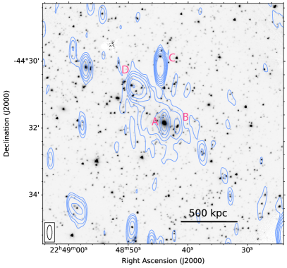
Figure 1: Spitzer 3.6 $\mu$m IRAC image of AS1063 overlaid with VLA 1.5 GHz radio contours. Contour levels are drawn at [1, 2, 4, 8, 16, 32] $\times$ 3$\sigma_{\rm rms}$, where $\sigma_{\rm rms}$ = 21 $\mu$Jy beam^-1. Due to the low declination of the cluster, the radio beam is quite elongated (26″$\times$ 9″). Compact radio sources are labelled A to D, see also Figure 7.

3 Results

3.1 Abell S1063

A Spitzer infrared (IR) image of AS1063, overlaid with our 1.5 GHz radio contours is presented in Figure 1. Four compact radio sources are detected in the cluster vicinity, labelled A to D in Figure 1. In the central regions of the cluster more extended diffuse emission is also detected. The properties of the radio sources are listed in Table 4.

Source A, namely rxj2248_17936 or 2MASX J22484405-4431507, is the BCG in AS1063. The integrated flux densities of the BCG are $8.5\pm 1.1$ mJy at 325 MHz, $2.1\pm 0.2$ mJy at 1.5 GHz, and $1.0\pm 0.1$ mJy at 3.0 GHz. This corresponds to a spectral index of about $-1$, typical for a cluster AGN. Source B (rxj2246_18112) is a background galaxy at redshift of 0.61, identified as [GVR2012] 878 by Gómez et al. (2012). Source C (rxj2248_19890) is the brightest radio galaxy in the cluster field, located north of the cluster center.

Source D (rxj2248_18479) is a radio galaxy with a radio tail at the northeast of the cluster. The radio tail is connected to the diffuse emission and the tail length is $\sim$140 kpc at 1.5 GHz (see, Figure 1). The tail length increase at 325 MHz to $\sim$340 kpc. The integrated flux densities are $37.8\pm 3.8$ mJy at 325 MHz, $5.6\pm 0.3$ mJy at 1.5 GHz, and $1.8\pm 0.1$ mJy at 3.0 GHz. The corresponding spectral indices are $\alpha^{1500}_{325}$ = -1.24 $\pm$ 0.07 and $\alpha^{3000}_{1500}$ = -1.61 $\pm$ 0.11. Such spectral behaviour indicates a high frequency break, the result of the radiative losses of the synchrotron emitting electrons.

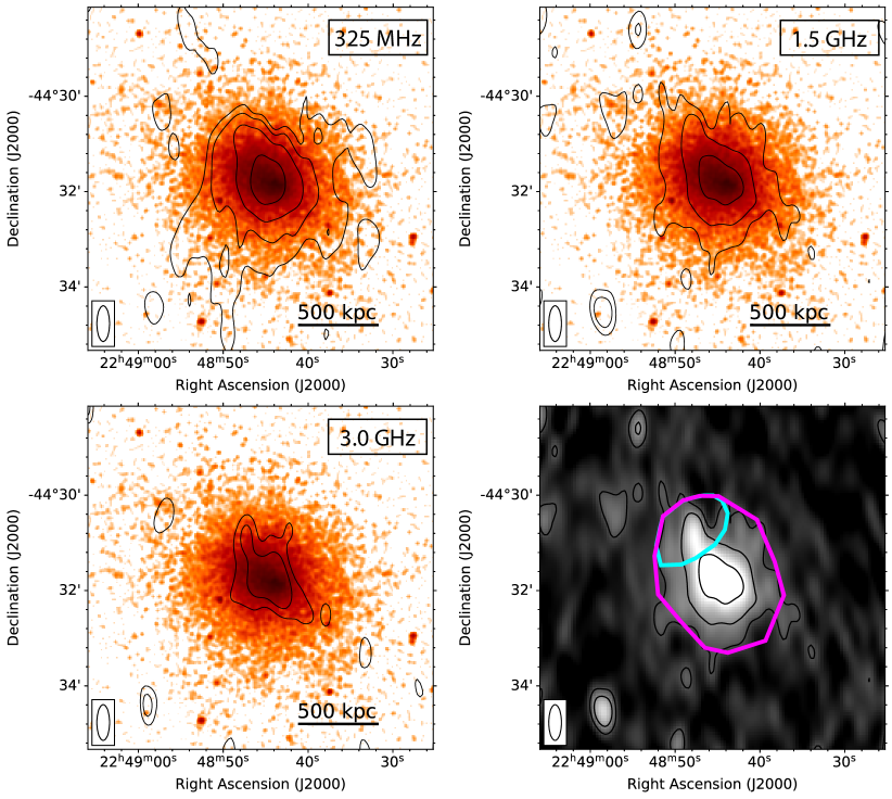
Figure 2: Chandra image of AS1063 overlaid with the radio contours of diffuse emission in AS1063 at three frequencies (325 MHz, top left; 1.5 GHz, top right; 3.0 GHz, bottom left). Chandra images are all in the energy band 0.5 – 2.0 keV with pixel size 4 $\times$ 0.492″and smoothed with a Gaussian with scale of 3 pixels across. Contour levels are drawn at [1, 2, 4, 8, …] $\times$ 3$\sigma_{\rm rms}$, where $\sigma_{\rm 325\leavevmode\nobreak\ MHz}$= 96 $\mu$Jy beam^-1, $\sigma_{\rm 1.5\leavevmode\nobreak\ GHz}$= 40 $\mu$Jy beam^-1, $\sigma_{\rm 3.0\leavevmode\nobreak\ GHz}$ = 24 $\mu$Jy beam^-1. Compact radio sources were subtracted in all radio images. The inner uv-cut of 0.15 k$\lambda$ is adopted for all radio images. Bottom right: VLA L-band image of AS1063 depicting the region where we extract the integrated flux densities. The cyan polygon indicates the region where the diffuse AGN component is subtracted from the total flux measurement (magenta polygon).

In Figure 2 we show the Chandra 0.5–2.0 keV X-ray image of the cluster. Radio contours at 0.325, 1.5 and 3.0 GHz are overlaid in the various panels. The emission from compact sources was subtracted from the uv-data in these radio images (see Sect. 2.3), to better determine the properties of the diffuse radio emission. Central diffuse emission is detected at all three frequencies which roughly follows the distribution of the thermal ICM. We further investigate the connection between the thermal and non-thermal emission by comparing the X-ray and radio surface brightness evaluated in the same regions of the Chandra 0.5-2.0 keV and GMRT 325 MHz source subtracted images. Regions were chosen based on the $3\sigma$ level emission of the GMRT image, where 19 beam independent regions were identified. The plot of the radio versus X-ray surface brightness is reported in Figure 3, where regions with higher X-ray surface brightness seems associated to regions with higher radio surface brightness. This trend has been observed for a number of radio halos (Govoni et al., 2001; Rajpurohit et al., 2018; Hoang et al., 2019; Cova et al., 2019). Despite the small number of data points, we fit the data with a power-law in the form $I_{\rm radio}\propto I_{\rm X-ray}^{b}$ and obtain a slope b = 0.55 $\pm$ 0.04 which is within the range of values found in the literature. From the 1.5 GHz image, a slope of $0.48\pm 0.07$ is obtained, which is consistent with the value from the 325 MHz image. The largest physical extent of the diffuse emission is $\sim$700 kpc at 1.5 GHz and this increases to $\sim$1.2 Mpc at 325 MHz. Besides the central diffuse emission, we also detect remnant emission from the tail of source D (also see, Figure 1). Because of the extended nature of the tail, it is not possible to fully remove this in the source subtraction processes. To determine the integrated flux density of the central diffuse emission we therefore exclude the area indicated by the cyan polygon in Figure 2 (bottom right panel). We used the same extraction region for the integrated flux density for all three frequencies (see Figure. 2). The uncertainties are computed as described in Sect. 2.3.

The flux densities of the central diffuse emission are $24.3\pm 2.5$ mJy, $5.8\pm 0.4$ mJy, and $1.7\pm 0.2$ mJy, at 325MHz, L-band, and S-band, respectively. Using the observed flux densities, we find that the spectral index steepens at high frequencies with $\alpha^{1500}_{325}=-0.94\leavevmode\nobreak\ \pm\leavevmode\nobreak\ 0.08$, and $\alpha^{3000}_{1500}=-1.77\leavevmode\nobreak\ \pm\leavevmode\nobreak\ 0.20$. If we adjust the size of the extraction region to the extension of the radio halo at 325 MHz, the derived spectral indices remain consistent with each other within the uncertainties. In Figure 4, we present the integrated spectrum of the diffuse emission. A single power-law fit is unacceptable with $\chi^{2}$/d.o.f. =17.7, showing the spectrum deviates from a power-law shape.

We conclude that the diffuse emission we find in AS1063 is a new radio halo based on the lack of a clear optical counterpart, the central location, and the large physical extent. From the flux density measurement in the L-band, we calculate a monochromatic radio halo power of $P_{\rm 1.4GHz}=(2.63\leavevmode\nobreak\ \pm\leavevmode\nobreak\ 0.18)\leavevmode\nobreak\ \times\leavevmode\nobreak\ 10^{24}$ W Hz^-1 using the equation

$$P_{\rm 1.4GHz}=4\pi D_{\rm L}^{2}S_{\rm 1.4GHz}(1+z)^{-(\alpha+1)},$$ (2)

where $D_{\rm L}$ is the luminosity distance. Here, we adopted $\alpha=-1.14$, and derived the flux density at 1.4 GHz $S_{\rm 1.4GHz}$ from $S_{\rm 1.5GHz}$ (scaling with the mentioned spectral index).

Statistical studies of radio halos have revealed a correlation between radio halo power and cluster mass (e.g., Cassano et al., 2006; Basu, 2012; Cassano et al., 2013; Sommer & Basu, 2014; Martinez Aviles et al., 2016). The general idea is that a small fraction of the gravitational energy is converted into relativistic electrons during a cluster merger. The amount of energy released correlates with the cluster mass and results in the relation between radio power and cluster mass. Adopting the cluster sample from Cassano et al. (2013), we over-plot our radio measurement of the halo emission on the $P_{\rm 1.4\leavevmode\nobreak\ GHz}$ - $Y_{\rm 500}$ diagram in Figure 5. $Y_{\rm 500}$ is the integrated SZ signal, estimated from Y${}_{5R_{500}}$ as Y₅₀₀ = Y${}_{5R_{500}}$ / 1.79 (Arnaud et al., 2010). The Y${}_{5R_{500}}$ is obtained from Planck Collaboration et al. (2016) . Unlike the X-ray luminosity, $Y_{\rm 500}$ is a more robust mass tracer as it less affected by the cluster’s dynamical state (Motl et al., 2005; Nagai, 2006). Figure 5 shows that the radio power of AS1063 is slightly lower than most clusters in this $Y_{\rm 500}$ range, but consistent within the expected scatter.

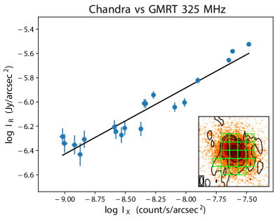
Figure 3: X-ray versus radio surface brightness (SB) for AS1063. The red line shows the best fit power-law $I_{\rm radio}\propto I_{\rm X-ray}^{0.55\pm 0.04}$. The inset shows the region (green grid) where we measured the corresponding surface brightness.

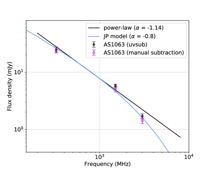
Figure 4: Integrated flux densities for the halo in AS1063 at 325 MHz, 1.5 GHz, and 3.0 GHz, measured by two methods. The black line shows a single power-law fit with spectral index $\alpha=-1.14$. The JP model has an injection spectral index of $-0.8$.

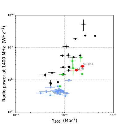
Figure 5: Distribution of radio halos in the $P_{\rm 1.4\leavevmode\nobreak\ GHz}$ - $Y_{\rm 500}$ diagram. Different symbols are used to represent the radio halos (black dots), radio halos with ultra-steep spectra (green dots) and the upper limits (blue arrows) from Cassano et al. (2013). AS1063 and A370 are shown as red dots.

Table 4: The properties of the radio sources for Abell S1063 and Abell 370, labelled in Figure 1 and Figure 8

Name	RA	Dec	$S_{\rm 325\leavevmode\nobreak\ MHz}$	$S_{\rm 1.5\leavevmode\nobreak\ GHz}$	$S_{\rm 3\leavevmode\nobreak\ GHz}$	$\alpha^{1500}_{325}$	$\alpha^{3000}_{1500}$
	(J2000)	(J2000)	(mJy)	(mJy)	(mJy)
AS1063 Halo(a)	22 48 43.5	-44 31 44.0	24.3 $\pm$ 2.5	5.8 $\pm$ 0.4	1.7 $\pm$ 0.2	-0.94 $\pm$ 0.08	-1.77 $\pm$ 0.20
AS1063 Source A	22 48 44.0	-44 31 51.85	8.5 $\pm$ 1.1	2.1 $\pm$ 0.2	1.0 $\pm$ 0.1	-0.93 $\pm$ 0.10	-1.03 $\pm$ 0.15
AS1063 Source B	22 48 41.8	-44 31 56.48	2.2 $\pm$ 0.3	0.7 $\pm$ 0.1	0.3 $\pm$ 0.1	-0.80 $\pm$ 0.12	-1.07 $\pm$ 0.23
AS1063 Source C	22 48 44.6	-44 30 09.59	40.7 $\pm$ 4.2	10.0 $\pm$ 0.5	4.5 $\pm$ 0.2	-0.92 $\pm$ 0.08	-1.16 $\pm$ 0.10
AS1063 Source D	22 48 49.3	-44 30 44.58	37.8 $\pm$ 3.8	5.6 $\pm$ 0.3	1.8 $\pm$ 0.1	-1.24 $\pm$ 0.07	-1.61 $\pm$ 0.11
A370 Halo(b)	02 39 52.0	-01 35 12.0	$20.0\pm 2.3$	$3.7\pm 0.3$	< 1.3	$-1.10\pm 0.09$	< $-1.51$
A370 Source A	02 39 52.7	-01 34 19.8	$0.9\pm 0.1$	$0.2\pm 0.1$	–	$-1.06\pm 0.18$	–
A370 Source B	02 39 53.1	-01 34 56.0	–	0.11 $\pm$ 0.01c	–	–	–
A370 Source C	02 39 50.9	-01 35 42.4	$3.1\pm 0.3$	$1.5\pm 0.1$	$0.8\pm 0.1$	$-0.48\pm 0.09$	$-0.91\pm 0.16$
A370 Source D	02 39 52.1	-01 35 56.8	$1.2\pm 0.6$	$0.3\pm 0.1$	$0.2\pm 0.1$	$-0.86\pm 0.34$	$-0.91\pm 0.75$
A370 Source E	02 39 55.4	-01 34 07.9	$15.5\pm 2.0$	$7.1\pm 0.7$	$4.4\pm 0.4$	$-0.51\pm 0.10$	$-0.70\pm 0.19$
A370 Source F	02 39 56.5	-01 34 29.0	$4.5\pm 1.0$	$2.0\pm 0.4$	$1.3\pm 0.1$	$-0.53\pm 0.19$	$-0.64\pm 0.28$

3.1.1 Spectral index maps

We constructed spectral index maps between 0.325 and 1.5 GHz, and between 1.5 and 3.0 GHz to characterize the spectral index distribution across the halo of AS1063 with resolution of $45\arcsec\times 16\arcsec$, see Figure 6. The imaging details can be found in Section 2.4. Spectral index uncertainty maps can be found in Appendix A.

The spectral index between 0.325 and 1.5 GHz ranges from $\sim$-0.8 at the eastern part of the halo to $\sim$-1.1 at the western part. The halo has steeper values between 1.5 GHz and 3.0 GHz, varying from $\sim$-1.7 at the eastern side to $\sim$-1.25 at the western side. However, these east-west trends are not very significant, considering the spectral index uncertainty of $\sim$0.15 and $\sim$0.25 in $\alpha^{1500}_{325}$ and $\alpha^{3000}_{1500}$ maps, respectively.

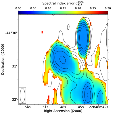
Figure 13: Spectral index uncertainty map of source D in AS1063 between 325 MHz and 1.5 GHz. The radio contours are from the 325 MHz image.

Figure 7 shows the spectral index map of source D between 325 MHz and 1.5 GHz. The corresponding uncertainty map can be found in Figure 13. Source D shows a clear spectral index gradient along the radio tail. The spectral index steepens from $\sim-0.6$ at location of the IR counterpart to $\sim-2.4$ at the tail end. Such a trend is expected as the result of the radiative losses of electrons.

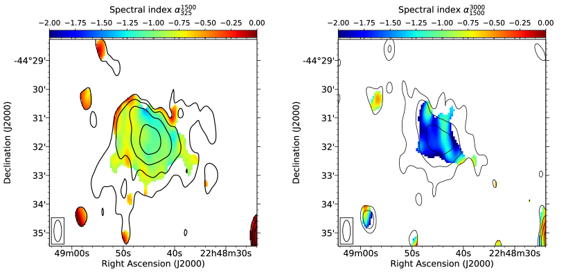
Figure 6: Spectral index maps of AS1063 between 325 MHz and 1.5 GHz (left), and between 1.5 GHz and 3.0 GHz (right). The radio contours are from the 325 MHz (left) and 1.5 GHz (right) images. These maps were created from the compact source subtracted uv-data. The beam size is indicated in the bottom left corner. Contour levels are drawn at [1, 2, 4, 8, …] $\times$ 3$\sigma_{\rm rms}$, where $\sigma_{\rm 325\leavevmode\nobreak\ MHz}$= 96 $\mu$Jy beam^-1, $\sigma_{\rm 1.5\leavevmode\nobreak\ GHz}$= 40 $\mu$Jy beam^-1.

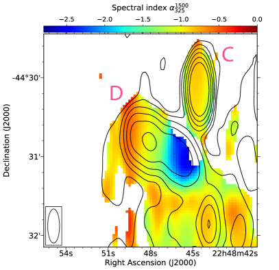
Figure 7: Spectral index map of source D in AS1063 between 325 MHz and 1.5 GHz. The radio contours are from the GMRT 325 MHz image. The beam size is 26.0″$\times$ 9.0″and indicated in the bottom left corner. Contour levels are drawn at [1, 2, 4, 8, 16, 32 …] $\times$ 5$\sigma_{\rm rms}$, where $\sigma_{\rm rms}$ = 46 $\mu$Jy beam^-1.

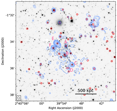
Figure 8: Spitzer 3.6 $\mu$m IRAC image of A370 overlaid with the GMRT 325 MHz radio contours. The beam size is 11.9″$\times$ 8.6″. Contour levels are drawn at [1, 2, 4, 8, 16, 32] $\times$ 3$\sigma_{\rm rms}$, where $\sigma_{\rm rms}$ = 62 $\mu$Jy beam^-1. Compact radio sources are indicated with red labels from A to F. The red circles mark the 1.4 GHz radio source catalog from Wold et al. (2012).

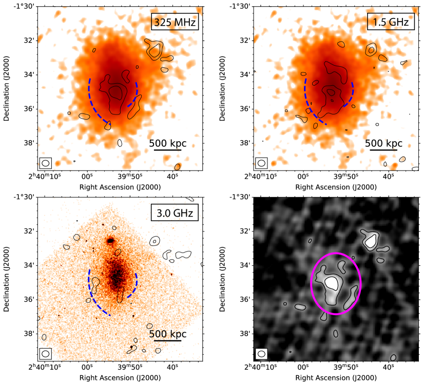
Figure 9: XMM-Newton 0.3–7 keV image of A370 overlaid with the radio contours with compact sources subtracted from the uv-data (325 MHz, top left; 1.5 GHz, top right). All the point source in XMM-Newton image are removed and smoothed with a Gaussian with scale of 3 pixels across. The Blue dashed curves show the surface brightness edges found by Botteon et al. (2018). Bottom left: Chandra 0.5–2.0 keV image overlaid with the 3.0 GHz radio contours with compact sources subtracted from the uv-data. The radio beam size is 25.0″$\times$ 22.0″. Contour levels are drawn at [1, 2, 4, 8, …] $\times$ 3$\sigma_{\rm rms}$, where $\sigma_{\rm 325\leavevmode\nobreak\ MHz}$= 161 $\mu$Jy beam^-1, $\sigma_{\rm 1.5\leavevmode\nobreak\ GHz}$= 34 $\mu$Jy beam^-1, $\sigma_{\rm 3.0\leavevmode\nobreak\ GHz}$ = 18 $\mu$Jy beam^-1. The inner uv-cut of 0.22 k$\lambda$ is adopted for 325 MHz and 1.5 GHz images. Bottom right: GMRT 325 MHz image of A370 depicting the region (magenta ellipse) where we extract the integrated flux densities.

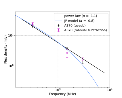
Figure 10: Integrated flux densities and 3$\sigma$ upper-limits for the halo in A370 at 325 MHz, 1.5 GHz, and 3.0 GHz, measured by two methods. The black line shows a single power-law with spectral index $\alpha=-1.1$. The JP model has an injection spectral index of $-0.8$.

3.2 Abell 370

A Spitzer image of A370 with 325 MHz radio contours overlaid is presented in Figure 8. A number of compact radio sources are detected in the cluster field. Wold et al. (2012) analyzed 1.4 GHz VLA observations of the A370 cluster field in the A and B configurations. Their radio source catalog is over plotted on Figure 8. We also label several radio sources in the cluster region, source A to F. The flux densities of these sources are reported in Table 4.

There are two BCGs in A370 and both show radio emission associated with an AGN. Source A, the northern BCG is detected at 325 MHz and 1.5 GHz. The flux densities are $S_{\rm 325\leavevmode\nobreak\ MHz}$ = $0.86\pm 0.10$ mJy and $S_{\rm 1.5\leavevmode\nobreak\ GHz}$ = $0.17\pm 0.04$ mJy, corresponding to a spectral index of $-1.06\pm 0.18$. The southern BCG marked as B, blends with other nearby radio sources in our relatively low resolution image with a beam size of 11.9″$\times$ 8.6″. The high resolution 1.4 GHz image of Wold et al. (2012) shows a separate radio source associated with the BCG with a flux density of 0.11 mJy.

Some very faint extended emission is found in the southern part of the cluster near source B and south of it (see Figure 8). To better bring out the diffuse emission we made low-resolution compact source subtracted images (for details see Section 2.3). A XMM-Newton X-ray image, with radio contours at 0.325 and 1.5 GHz overlaid, is displayed in Figure 9. For completeness, a Chandra image is also shown, overlaid with radio contours at 3 GHz. Diffuse emission is detected at 325 MHz and 1.5 GHz. The total extent of the diffuse emission is about 500–700 kpc. The surface brightness of this emission peaks at the location of the southern BCG. Note that the emission at north-west periphery of the cluster are residuals from an extended tailed radio galaxy that is not completely subtracted from uv-data. The flux density of the radio halo is $20.0\pm 2.3$ mJy at 325 MHz and $3.7\pm 0.3$ mJy at 1.5 GHz. For the non-detection at 3.0 GHz we determine a $3\sigma$ upper limit of < 1.3 mJy. The region where we measured the flux densities is indicated in Figure 9. The corresponding spectral indices are $\alpha^{1500}_{325}=-1.10\leavevmode\nobreak\ \pm\leavevmode\nobreak\ 0.09$, and $\alpha^{3000}_{1500}<-1.51$.

We classify the extended emission in A370 as a radio halo based on the lack of a clear optical counterpart, physical extent, and location in the cluster. Deeper observations will be needed to determine the full extent of the radio halo given its low surface brightness. We compute a monochromatic radio power at 1.4 GHz of $P_{\rm 1.4GHz}=(2.00\leavevmode\nobreak\ \pm\leavevmode\nobreak\ 0.16)\leavevmode\nobreak\ \times\leavevmode\nobreak\ 10^{24}$ W Hz^-1, where we take $\alpha=-1.1$. The radio halo power is consistent with that expected from the known scaling relations (Cassano et al., 2013), see Figure 5. We do not compute spectral index maps of the radio halo as the emission is barely detected at three times the map noise level.

Botteon et al. (2018) detected two X-ray surface brightness edges on the west and east side of the cluster, shown as blue dashed curves in Figure 9. Due to the limited number of X-ray counts, the nature (cold front or shock) of these edges could not be determined. No clear correspondence between the edges and radio emission halo emission is found.

4 Discussion

4.1 Merger scenarios and nature of the radio halos

The presence of a radio halo in the massive merging cluster A370 is expected based on the dynamical state of this cluster. A370 has a clear bimodal mass distribution, indicating a major merger event (Richard et al., 2010). This is also supported by the presence of X-ray surface brightness edges (Botteon et al., 2018). The radio halo in A370 thus supports the general scenario that radio halos trace particles that are re-accelerated by merger induced turbulence.

The dynamical state of AS1063 is key to interpreting the nature and formation scenario for its radio halo. However, the dynamical state of AS1063 is still under debate. The presence of a single BCG and a morphological analysis from XMM-Newton observations suggest a relaxed dynamical state (Lovisari et al., 2017). This X-ray analysis used the concentration value, power ratio, and centroid shift. On the other hand the offset between the galaxy distribution and the peak of the X-ray emission, high global X-ray temperature, and weak lensing analysis indicate an ongoing major merger event (Gómez et al., 2012; Gruen et al., 2013).

Radio mini-halos exclusively occur in cool core clusters. In addition, typically their sizes are a few hundreds of kpc and the emission from the mini-halo is confined to the cooling region (e.g., Mazzotta & Giacintucci, 2008; Giacintucci et al., 2017, 2019). To determine whether AS1063 hosts a cool core we derived a radial temperature profile from the XMM-Newton data, see Sect. 2.5 for more details. This radial profile is displayed in Figure 11. The central two bins of this profile (< 250 kpc) show temperatures about 10 keV which indicate AS1063 has a rather hot-core. This result is consistent with the conclusion of the presence of a hot-core based on Chandra data by Gómez et al. (2012). We thus conclude that the diffuse emission in AS1063 cannot be classified as a radio mini-halo, also in line with the rather large extent of the halo. The presence of the giant radio halo ($\sim$1.2 Mpc) in AS1063 therefore suggests a link to a cluster merger event. In line with the previous claims of an on-going merger by Gómez et al. (2012); Gruen et al. (2013).

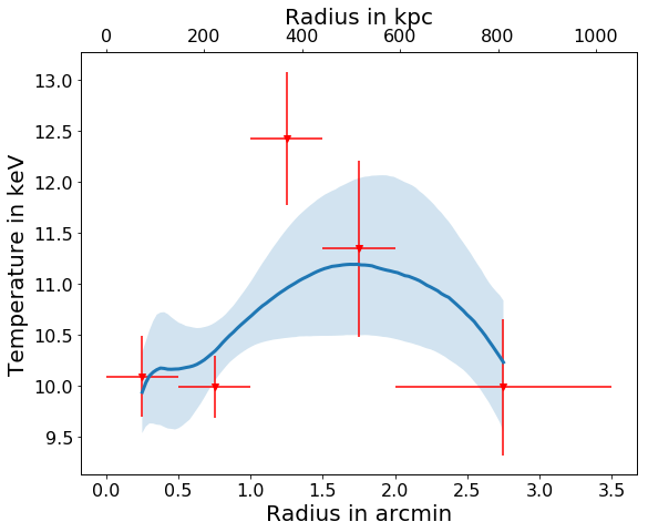
Figure 11: The radial temperature profile of AS1063 obtained from XMM-Newton observations (Lovisari et al. in prep.). The size of the bins was set to be $\geq$ 30″ to limit the scatter of photons from bin to bin. The observed projected temperatures are shown by red points. The blue line and shaded area show the best-fit projected profile and its 1$\sigma$ uncertainty computed by using the best-fit three-dimensional model described in Vikhlinin et al. (2006).

4.2 Curved radio spectra

The radio spectra of halos provide important information about the underlying particle (re-)acceleration mechanisms. According to the turbulent re-acceleration model, we expect a cutoff in the energy spectrum of the CR electrons which also leads to a cutoff in the synchrotron emission above a certain frequency (e.g., Brunetti & Jones, 2014). However, only a few clusters have been found that show this spectral steepening. Some examples are the Coma Cluster (Schlickeiser et al., 1987; Thierbach et al., 2003) and Abell 3562 (Giacintucci et al., 2005). A possible explanation for why very few clusters show spectral curvature are the observational difficulties involved. High quality flux density measurements at wide enough frequency spacing are hard to obtain. In addition, the magnetic field properties and amount of turbulence will differ with location in the ICM. These inhomogeneous conditions result in spectra with different local cutoff frequencies. The spectral curvature will therefore be less pronounced for the integrated spectra when these inhomogeneous conditions are present (e.g., ZuHone et al., 2013; Donnert et al., 2013; Pinzke et al., 2017).

Our flux density measurements of AS1063 show spectral steepening between 1.5 and 3 GHz, providing support for the turbulent re-acceleration model. To characterize the spectral steepening, we compare our flux measurements to a Jaffe & Perola (1973) (JP) model with a “reasonable” injection spectral index of $-0.8$ (Thierbach et al., 2003) in Figures 4 and 10. A comparison with a JP model is useful here since a JP spectrum has a power-law shape with an exponential cutoff. The amount of spectral steepening for AS1063 is quite strong and well described by exponential cutoff. This would indicate that ICM conditions in AS1063 are rather homogeneous leading to similar cutoff frequencies at different spatial positions. For A370, the measurement uncertainties do not allow us to draw firm conclusions on the amount of spectral steepening.

It is important to stress that the observed spectral curvature for AS1063 is completely based on one measurement at 3 GHz. Therefore, future observations are important to confirm this result and characterize the shape of the radio spectrum in more detail. We note that the relatively small spatial extent (3′) and relatively high surface brightness of the AS1063 radio halo make it a promising target for future observations with the VLA at 4–8 GHz and at $\lesssim 1$ GHz with the uGMRT.

5 Conclusions

In this paper, we presented 325 MHz GMRT and 1–4 GHz VLA observations of the Frontier Fields clusters AS1063 and A370. The results are summarized below:

1. We discovered a giant $\sim$1.2 Mpc radio halo in AS1063. The radio halo roughly follows the X-ray emission from the thermal ICM. We determined a radio halo power of $P_{\rm 1.4GHz}=(2.63\pm 0.18)\times 10^{24}$ W Hz^-1.

2. The integrated spectral index of the AS1063 radio halo measures $-0.94\pm 0.08$ between 0.325 and 1.5 GHz and it steepens to $-1.77\pm 0.20$ between 1.5 GHz and 3.0 GHz. This spectral steepening provides support for the turbulent re-acceleration model for the formation of radio halos.

3. We discovered a faint radio halo in A370 with a size of about 500–700 kpc. The radio halo power is $P_{\rm 1.4GHz}=(2.00\pm 0.16)\times 10^{24}$ W Hz^-1. The radio halo is not detected at 3.0 GHz, with a 3$\sigma$ limit of 1.3 mJy. We measure a spectral index of $-1.10\leavevmode\nobreak\ \pm\leavevmode\nobreak\ 0.09$ between 0.325 and 1.5 GHz.

4. The radio halo powers of AS1063 and A370 follow the $P_{\rm 1.4\leavevmode\nobreak\ GHz}$ - $Y_{\rm 500}$ scaling relation. Complementing our radio data with Chandra and XMM-Newton X-ray observations provides support for the idea that both radio halos are related to ongoing cluster merger events.

Appendix A The spectral index uncertainty maps

Figures 12 and 13 show the uncertainty maps corresponding to the spectral index maps in Figures 6 and 7, respectively.

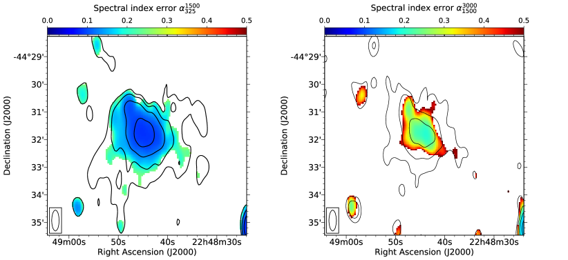
Figure 12: Spectral index uncertainty maps of AS1063 between 325 MHz and 1.5 GHz (left), and between 1.5 GHz and 3.0 GHz (right). The radio contours are from the 325 MHz (left) and 1.5 GHz (right) images.

References

- Abell et al. (1989) Abell, G. O., Corwin, Jr., H. G., & Olowin, R. P. 1989, ApJS, 70, 1
- Ackermann et al. (2014) Ackermann, M., Ajello, M., Albert, A., et al. 2014, ApJ, 787, 18
- Ackermann et al. (2016) Ackermann, M., Ajello, M., Albert, A., et al. 2016, ApJ, 819, 149
- Arnaud et al. (2010) Arnaud, M., Pratt, G. W., Piffaretti, R., et al. 2010, A&A, 517, A92
- Astropy Collaboration et al. (2013) Astropy Collaboration, Robitaille, T. P., Tollerud, E. J., et al. 2013, A&A, 558, A33
- Basu (2012) Basu, K. 2012, MNRAS, 421, L112
- Blasi & Colafrancesco (1999) Blasi, P. & Colafrancesco, S. 1999, Astroparticle Physics, 12, 169
- Bonafede et al. (2009) Bonafede, A., Giovannini, G., Feretti, L., Govoni, F., & Murgia, M. 2009, A&A, 494, 429
- Botteon et al. (2018) Botteon, A., Gastaldello, F., & Brunetti, G. 2018, MNRAS, 476, 5591
- Briggs (1995) Briggs, D. S. 1995, PhD thesis, New Mexico Institute of Mining Technology, Socorro, www.atnf.csiro.au/people/tim.cornwell/research/danthesis.pdf
- Broadhurst et al. (2008) Broadhurst, T., Umetsu, K., Medezinski, E., Oguri, M., & Rephaeli, Y. 2008, ApJ, 685, L9
- Brown & Rudnick (2011) Brown, S. & Rudnick, L. 2011, MNRAS, 412, 2
- Brunetti et al. (2008) Brunetti, G., Giacintucci, S., Cassano, R., et al. 2008, Nature, 455, 944
- Brunetti & Jones (2014) Brunetti, G. & Jones, T. W. 2014, International Journal of Modern Physics D, 23, 1430007
- Brunetti et al. (2001) Brunetti, G., Setti, G., Feretti, L., & Giovannini, G. 2001, MNRAS, 320, 365
- Brunetti et al. (2017) Brunetti, G., Zimmer, S., & Zandanel, F. 2017, MNRAS, 472, 1506
- Cassano et al. (2006) Cassano, R., Brunetti, G., & Setti, G. 2006, MNRAS, 369, 1577
- Cassano et al. (2013) Cassano, R., Ettori, S., Brunetti, G., et al. 2013, ApJ, 777, 141
- Cassano et al. (2010) Cassano, R., Ettori, S., Giacintucci, S., et al. 2010, ApJ, 721, L82
- Cornwell (2008) Cornwell, T. J. 2008, IEEE Journal of Selected Topics in Signal Processing, 2, 793
- Cova et al. (2019) Cova, F., Gastaldello, F., Wik, D. R., et al. 2019, A&A, 628, A83
- Cuciti et al. (2018) Cuciti, V., Brunetti, G., van Weeren, R., et al. 2018, A&A, 609, A61
- Dennison (1980) Dennison, B. 1980, ApJ, 239, L93
- Donnert et al. (2013) Donnert, J., Dolag, K., Brunetti, G., & Cassano, R. 2013, MNRAS, 429, 3564
- Feretti et al. (2012) Feretti, L., Giovannini, G., Govoni, F., & Murgia, M. 2012, A&A Rev., 20, 54
- Fujita et al. (2007) Fujita, Y., Kohri, K., Yamazaki, R., & Kino, M. 2007, ApJ, 663, L61
- Fujita & Ohira (2013) Fujita, Y. & Ohira, Y. 2013, MNRAS, 428, 599
- Giacintucci et al. (2017) Giacintucci, S., Markevitch, M., Cassano, R., et al. 2017, ApJ, 841, 71
- Giacintucci et al. (2019) Giacintucci, S., Markevitch, M., Cassano, R., et al. 2019, ApJ, 880, 70
- Giacintucci et al. (2005) Giacintucci, S., Venturi, T., Brunetti, G., et al. 2005, A&A, 440, 867
- Giovannini et al. (1993) Giovannini, G., Feretti, L., Venturi, T., Kim, K. T., & Kronberg, P. P. 1993, ApJ, 406, 399
- Gómez et al. (2012) Gómez, P. L., Valkonen, L. E., Romer, A. K., et al. 2012, AJ, 144, 79
- Govoni et al. (2001) Govoni, F., Feretti, L., Giovannini, G., et al. 2001, A&A, 376, 803
- Govoni et al. (2004) Govoni, F., Markevitch, M., Vikhlinin, A., et al. 2004, ApJ, 605, 695
- Gruen et al. (2013) Gruen, D., Brimioulle, F., Seitz, S., et al. 2013, MNRAS, 432, 1455
- Hart et al. (2009) Hart, Q. N., Stocke, J. T., & Hallman, E. J. 2009, ApJ, 705, 854
- Hoag (1981) Hoag, A. 1981, in BAAS, Vol. 13, Bulletin of the American Astronomical Society, 799
- Hoang et al. (2019) Hoang, D. N., Shimwell, T. W., van Weeren, R. J., et al. 2019, A&A, 622, A20
- Intema (2014) Intema, H. T. 2014, in Astronomical Society of India Conference Series, Vol. 13, Astronomical Society of India Conference Series
- Intema et al. (2017) Intema, H. T., Jagannathan, P., Mooley, K. P., & Frail, D. A. 2017, A&A, 598, A78
- Intema et al. (2009) Intema, H. T., van der Tol, S., Cotton, W. D., et al. 2009, A&A, 501, 1185
- Jaffe & Perola (1973) Jaffe, W. J. & Perola, G. C. 1973, A&A, 26, 423
- Kale et al. (2019) Kale, R., Shende, K. M., & Parekh, V. 2019, MNRAS, 486, L80
- Kale et al. (2015) Kale, R., Venturi, T., Giacintucci, S., et al. 2015, A&A, 579, A92
- Keshet & Loeb (2010) Keshet, U. & Loeb, A. 2010, ApJ, 722, 737
- Kneib et al. (1993) Kneib, J. P., Mellier, Y., Fort, B., & Mathez, G. 1993, A&A, 273, 367
- Lagattuta et al. (2017) Lagattuta, D. J., Richard, J., Clément, B., et al. 2017, MNRAS, 469, 3946
- Lah et al. (2009) Lah, P., Pracy, M. B., Chengalur, J. N., et al. 2009, MNRAS, 399, 1447
- Liang et al. (2000) Liang, H., Hunstead, R. W., Birkinshaw, M., & Andreani, P. 2000, ApJ, 544, 686
- Lotz et al. (2017) Lotz, J. M., Koekemoer, A., Coe, D., et al. 2017, ApJ, 837, 97
- Lovisari et al. (2017) Lovisari, L., Forman, W. R., Jones, C., et al. 2017, ApJ, 846, 51
- Lovisari & Reiprich (2019) Lovisari, L. & Reiprich, T. H. 2019, MNRAS, 483, 540
- Lovisari et al. (2011) Lovisari, L., Schindler, S., & Kapferer, W. 2011, A&A, 528, A60
- Lynds & Petrosian (1986) Lynds, R. & Petrosian, V. 1986, in BAAS, Vol. 18, Bulletin of the American Astronomical Society, 1014
- Martinez Aviles et al. (2016) Martinez Aviles, G., Ferrari, C., Johnston-Hollitt, M., et al. 2016, A&A, 595, A116
- Mazzotta & Giacintucci (2008) Mazzotta, P. & Giacintucci, S. 2008, ApJ, 675, L9
- Mohan & Rafferty (2015) Mohan, N. & Rafferty, D. 2015, PyBDSF: Python Blob Detection and Source Finder, Astrophysics Source Code Library
- Morandi et al. (2007) Morandi, A., Ettori, S., & Moscardini, L. 2007, MNRAS, 379, 518
- Motl et al. (2005) Motl, P. M., Hallman, E. J., Burns, J. O., & Norman, M. L. 2005, ApJ, 623, L63
- Nagai (2006) Nagai, D. 2006, ApJ, 650, 538
- Offringa et al. (2010) Offringa, A. R., de Bruyn, A. G., Biehl, M., et al. 2010, MNRAS, 405, 155
- Paczynski (1987) Paczynski, B. 1987, Nature, 325, 572
- Pearce et al. (2017) Pearce, C. J. J., van Weeren, R. J., Andrade-Santos, F., et al. 2017, ApJ, 845, 81
- Perley & Butler (2013) Perley, R. A. & Butler, B. J. 2013, ApJS, 204, 19
- Petrosian (2001) Petrosian, V. 2001, ApJ, 557, 560
- Pfrommer & Enßlin (2004) Pfrommer, C. & Enßlin, T. A. 2004, A&A, 413, 17
- Pinzke et al. (2017) Pinzke, A., Oh, S. P., & Pfrommer, C. 2017, MNRAS, 465, 4800
- Planck Collaboration et al. (2016) Planck Collaboration, Ade, P. A. R., Aghanim, N., et al. 2016, A&A, 594, A27
- Postman et al. (2012) Postman, M., Coe, D., Benítez, N., et al. 2012, ApJS, 199, 25
- Price-Whelan et al. (2018) Price-Whelan, A. M., Sipőcz, B. M., Günther, H. M., et al. 2018, AJ, 156, 123
- Rajpurohit et al. (2018) Rajpurohit, K., Hoeft, M., van Weeren, R. J., et al. 2018, ApJ, 852, 65
- Rau & Cornwell (2011) Rau, U. & Cornwell, T. J. 2011, A&A, 532, A71
- Richard et al. (2010) Richard, J., Kneib, J.-P., Limousin, M., Edge, A., & Jullo, E. 2010, MNRAS, 402, L44
- Robitaille (2019) Robitaille, T. 2019, APLpy v2.0: The Astronomical Plotting Library in Python
- Robitaille & Bressert (2012) Robitaille, T. & Bressert, E. 2012, APLpy: Astronomical Plotting Library in Python, Astrophysics Source Code Library
- Savini et al. (2019) Savini, F., Bonafede, A., Brüggen, M., et al. 2019, A&A, 622, A24
- Scaife & Heald (2012) Scaife, A. M. M. & Heald, G. H. 2012, MNRAS, 423, L30
- Schlickeiser et al. (1987) Schlickeiser, R., Sievers, A., & Thiemann, H. 1987, A&A, 182, 21
- Sijbring & de Bruyn (1998) Sijbring, D. & de Bruyn, A. G. 1998, A&A, 331, 901
- Smail et al. (1996) Smail, I., Dressler, A., Kneib, J.-P., et al. 1996, ApJ, 469, 508
- Smail et al. (2000) Smail, I., Ivison, R. J., Owen, F. N., Blain, A. W., & Kneib, J.-P. 2000, ApJ, 528, 612
- Sommer & Basu (2014) Sommer, M. W. & Basu, K. 2014, MNRAS, 437, 2163
- Soucail et al. (1987) Soucail, G., Fort, B., Mellier, Y., & Picat, J. P. 1987, A&A, 172, L14
- Strait et al. (2018) Strait, V., Bradač, M., Hoag, A., et al. 2018, ApJ, 868, 129
- Struble & Rood (1999) Struble, M. F. & Rood, H. J. 1999, ApJS, 125, 35
- Thierbach et al. (2003) Thierbach, M., Klein, U., & Wielebinski, R. 2003, A&A, 397, 53
- Umetsu et al. (2011) Umetsu, K., Broadhurst, T., Zitrin, A., et al. 2011, ApJ, 738, 41
- van Weeren et al. (2016a) van Weeren, R. J., Brunetti, G., Brüggen, M., et al. 2016a, ApJ, 818, 204
- van Weeren et al. (2019) van Weeren, R. J., de Gasperin, F., Akamatsu, H., et al. 2019, Space Sci. Rev., 215, 16
- van Weeren et al. (2016b) van Weeren, R. J., Ogrean, G. A., Jones, C., et al. 2016b, ApJ, 817, 98
- van Weeren et al. (2017) van Weeren, R. J., Ogrean, G. A., Jones, C., et al. 2017, ApJ, 835, 197
- van Weeren et al. (2009) van Weeren, R. J., Röttgering, H. J. A., Bagchi, J., et al. 2009, A&A, 506, 1083
- vanWeeren et al. (2014) vanWeeren, R. J., Intema, H. T., Lal, D. V., et al. 2014, ApJ, 786, L17
- Venturi et al. (2007) Venturi, T., Giacintucci, S., Brunetti, G., et al. 2007, A&A, 463, 937
- Vikhlinin et al. (2006) Vikhlinin, A., Kravtsov, A., Forman, W., et al. 2006, ApJ, 640, 691
- Vikhlinin et al. (2005) Vikhlinin, A., Markevitch, M., Murray, S. S., et al. 2005, ApJ, 628, 655
- Williamson et al. (2011) Williamson, R., Benson, B. A., High, F. W., et al. 2011, ApJ, 738, 139
- Wold et al. (2012) Wold, I. G. B., Owen, F. N., Wang, W.-H., Barger, A. J., & Keenan, R. C. 2012, ApJS, 202, 2
- ZuHone et al. (2013) ZuHone, J. A., Markevitch, M., Brunetti, G., & Giacintucci, S. 2013, ApJ, 762, 78