Nullspace Vertex Partition in Graphs

Abstract

The core vertex set of a graph is an invariant of the graph. It consists of those vertices associated with the non-zero entries of the nullspace vectors of a $\{0,1\}$-adjacency matrix. The remaining vertices of the graph form the core–forbidden vertex set. For graphs with independent core vertices, such as bipartite minimal configurations and trees, the nullspace induces a well defined three part vertex partition. The parts of this partition are the core vertex set, their neighbours and the remote core–forbidden vertices. The set of the remote core–forbidden vertices are those not adjacent to any core vertex. We show that this set can be removed, leaving the nullity unchanged. For graphs with independent core vertices, we show that the submatrix of the adjacency matrix defining the edges incident to the core vertices determines the nullity of the adjacency matrix. For the efficient allocation of edges in a network graph without altering the nullity of its adjacency matrix, we determine which perturbations make up sufficient conditions for the core vertex set of the adjacency matrix of a graph to be preserved in the process.

Keywords Nullspace, core vertices, core–labelling, graph perturbations.

Mathematics Classification 202105C50, 15A18

1 Introduction

A graph $G=(V,E)$ has a finite vertex set $V=\{v_{1},v_{2},\ldots,v_{n}\}$ with vertex labelling $[n]:=\{1,2,...,n\}$ and an edge set $E$ of 2-element subsets of $V$. The graphs we consider are simple, that is without loops or multiple edges. A subset $U$ of $V$ is independent if no two vertices form an edge. The open–neighbourhood of a vertex $v\in V$, denoted by $N(v)$, is the set of all vertices incident to $v$. The degree $\rho(v)$ of a vertex $v$ is the number of edges incident to $v$. The induced subgraph $G[V\backslash S]$ of $G$ is $G-S$ obtained by deleting a vertex subset $S,$ together with the edges incident to the vertices in $S$. For simplicity of notation, we write $G-u$ for the induced subgraph obtained from $G$ by deleting vertex $u$ and $G-u-w$ when both vertices $u$ and $w$ are deleted.

The adjacency matrix $\mathbf{A}=(a_{ij})$ of the labelled graph $G$ on $n$ vertices is the $n\times n$ matrix $\mathbf{A}=(a_{ij})$ such that $a_{ij}=1$ if the vertices $v_{i}$ and $v_{j}$ are adjacent (that is $v_{i}\sim v_{j}$) and $a_{ij}=0$ otherwise. The nullity $\eta(G)$ is the algebraic multiplicity of the eigenvalue $0$ of $\mathbf{A}$, obtained as a root of the characteristic polynomial $\det(\lambda{\bf I}-{\bf A})$. The geometric multiplicity of an eigenvalue of a matrix is the dimension $\eta({\bf A})$ of the nullspace $\ker({\bf A})$ of ${\bf A}.$ Since ${\bf A}$ is real and symmetric, it is the same as its algebraic multiplicity. In particular, the nullity $\eta(G)$ of $G$ is the multiplicity of the eigenvalue 0. By the dimension theorem for linear transformations, for a graph $G$ on $n$ vertices, the rank of ${\bf A}$ is $\text{rank}(G)=n-\eta(G)$. Graphs, for which 0 is an eigenvalue, that is $\eta(G)>0,$ are singular.

In [3, 4, 5], the terms core vertex, core–forbidden vertex and kernel vector for a singular graph $G$ are introduced. The kernel vector refers to a non–zero vector $\mathbf{x}$ in the nullspace of $\mathbf{A},$ that is, it satisfies $\mathbf{A}\mathbf{x}=\mathbf{0}$, $\mathbf{x}\neq\mathbf{0}$. The support of a vector $\mathbf{x}$ is the set of indices of non–zero entries of ${\bf x}$.

Definition 1.

[4, 6] A vertex of a singular graph $G$ is a core vertex $(cv)$ of $G$ if it corresponds to a non-zero entry of some kernel vector of $G$. A vertex $u$ is a core–forbidden vertex $(cfv)$, if every kernel vector has a zero entry at position $u.$

It follows that the union of the elements of the support of all kernel vectors of ${\bf A}$ form the set of core vertices of $G.$ It is clear that a vertex of a singular graph $G$ is either a $cv$ or a $cfv$. The set of core vertices is denoted by $CV$, and the set ${\mathcal{V}}\backslash CV$ by $CFV$.

Cauchy’s Inequalities for real symmetric matrices, also referred to as the Interlacing Theorem in spectral graph theory [13], are considered to be among the most powerful tool in studies related to the location of eigenvalues. The Interlacing Theorem refers to the interlacing of the eigenvalues of the adjacency matrix of a vertex deleted subgraph relative to those of the parent graph.

As a consequence of the well-known Interlacing Theorem, the nullity of a graph can change by 1 at most, on deleting a vertex.

On deleting a vertex, the nullity reduces by 1 if and only if the vertex is a core vertex [15, Proposition 1.4], [7, Corollary 13] and [8, Theorem 2.3]. It follows that the deletion of a core–forbidden vertex can leave the nullity of the adjacency matrix unchanged, or else the nullity increases by 1.

Definition 2.

A vertex of a graph $G$ is $cfv_{mid}$ if its deletion leaves the nullity of the adjacency matrix, of the subgraph obtained, unchanged. A vertex of $G$ is $cfv_{upp}$ if when removed, the nullity increases by 1. The set $CFV$ is the disjoint union of the sets $\left\{cfv_{mid}\right\}$ and $\left\{cfv_{upp}\right\}$, denoted by $CFV_{mid}$ and $CFV_{upp},$ respectively.

At this point it is worth mentioning that in 1994, the first author coined the phrases core vertices, periphery and core-forbidden vertices. The core vertices with respect to ${\bf x}$ of a graph $G$ with a singular adjacency matrix ${\bf A}$ correspond to the support of the vector ${\bf x}$ in the nullspace of ${\bf A}$. One must not confuse the core vertex set with the same term referring to independent sets introduced much later [9]. The term core is also used in relation to graph homomorphisms.

There were other researchers who used associated concepts in different contexts. In 1982, Neumaier used the terms essential and non–essential vertices corresponding to core vertices and core–forbidden vertices, respectively, but only for the class of trees [10]. Back in 1960, S. Parter studied the upper core–forbidden vertices in the context of real symmetric matrices. In fact in the linear algebraic community these vertices are referred to as Parter vertices, the core vertices as downer vertices and the middle core–forbidden vertices as neutral vertices. Core–forbidden vertices are also referred to as Fiedler vertices in engineering.

Graphs with no edges between pairs of vertices in CV have a well defined vertex partition, which facilitates the form of the adjacency matrix in block form as shown in (1) in Section 3.

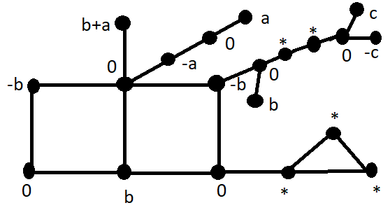
Figure 1: A vertex partition induced by a generalized kernel vector of $G$ in a graph of nullity 3: the label 0 indicates a vertex in $N(CV)$; the starred vertices are $cfv_{R}$.

Definition 3.

A graph is said to have independent core vertices if no two core vertices are adjacent.

If CV is an independent set, then the core-forbidden vertex set $CFV$ is partitioned into two subsets: $N(CV),$ the neighbours of the core vertices in $G$, and $CFV_{R},$ the remote core–forbidden vertices, as shown in Figure 1 for a graph of nullity 3. A similar concept is considered in [14, 16] for the case of trees. In this work, unless specifically stated, we consider all graphs.

Definition 4.

A core-labelled graph $G$ has an independent CV. The vertex set of $G$ is partitioned such that $V=CV\ \dot{\cup}\ N(CV)\ \dot{\cup}\ CFV_{R}$. The vertices of $CV$ are labelled first, followed by those of $N(CV)$ and then by those of $CFV_{R}.$

In Section 2, we show that removing a pendant edge from a graph not only preserves the nullity (which is well known) but also the type of vertices.

In Section 3, we determine the nullity of the submatrices of the adjacency matrix for a graph in the class of graphs with independent core vertices. The remote core–forbidden vertices do not contribute to the equations involving the nullspace vectors and can be removed to obtain a slim graph. In Section 4, bipartite minimal configurations are shown to be slim graphs with independent core vertices. Moreover all vertices in $N(CV)$ of a bipartite minimal configuration are shown to be upper core–forbidden vertices. In Section 5, we obtain results on the nullity and the number of the different types of vertices of singular trees in the light of the results obtained in Section 3. Section 6 focuses on the types of non–adjacent vertex pairs that can be joined by edges in a graph under various constraints associated with the nullspace of ${\bf A}.$

2 Graphs with Pendant Edges

By definition of $CV$ and $CFV,$ the nullspace of $\bf A$ induces a partition of the vertices of the associated graph $G$ into $CV$ and $CFV.$ The set $CV$ is empty if $G$ is non–singular and non–empty otherwise. It could happen that $CFV$ is empty in which case the graph is singular and it is a core graph. Consider two graphs on 4 vertices. The path $P_{4}$ is non–singular whereas the cycle $C_{4}$ is a core graph of nullity two.

A quick method to obtain the nullity and kernel vectors of a graph is known as the Zero Sum Rule. The neighbours of a vertex are weighted so that their weights add up to zero. Repeating this for each vertex gives the minimum number $\eta(G)$ of independent parameters in which to express the entries of a generalized vector in the nullspace of ${\bf A}$. Figure 2 shows a graph of nullity two with the entry of a generalized kernel vector next to each vertex, in terms of the parameters $a$ and $b$.

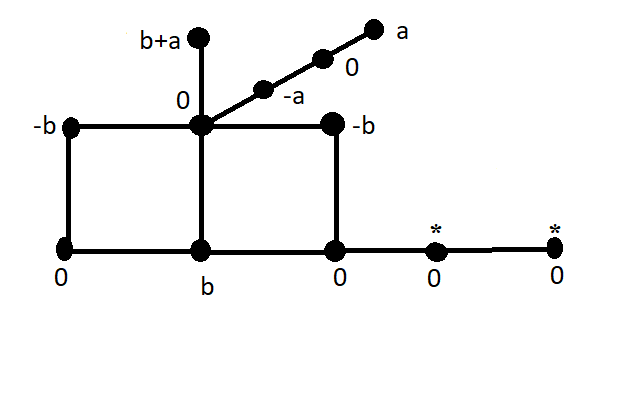
Figure 2: A graph of nullity 2 and a generalized kernel vector ${\bf x}(a,b)$ of $G$. The labels in terms of $a$ and $b$ identify the core vertices; the label 0 indicates core–forbidden vertices.

We are interested in the change in the type of vertices on the deletion of vertices and edges. Deleting a core–vertex from an odd path $P_{2k+1}$ may transform some of the core vertices to $CFV_{upp}$. Similarly, deleting a $CFV_{upp}$ vertex from the cycle $C_{6}$ on six vertices transforms some of the core–forbidden vertices to core–vertices. Removing a core vertex and a neighbouring $cfv$ may alter the nullity. Consider the 4 vertex graph obtained by identifying an edge of two 3–cycles. Removing the identified edge increases the nullity by 1, whereas removing any of the other edges decreases the nullity by 1.

However, it is well known that removing an end vertex $v,$ also known as a leaf, in the literature, and its unique neighbour $u,$ from a graph $G$, leaves the nullity unchanged in $G-u-v$ [21]. Note that the vertex $v$ may be $cv$ or $cfv.$ We give a new proof of this known result that also leads to an unusual preservation of the type of the remaining vertices after removing two vertices.

Theorem 5.

Let $w$ be an end vertex and $u$ its unique neighbour in a singular graph $G$. The nullity of $G-u-w$ is the same as that of $G$. Moreover, the type of vertices in $G-u-w$ is preserved.

Proof.

Let $u,w$ be the $n-1^{\text{th}}$ and $n^{\text{th}}$ labelled vertices, respectively, of a graph on $n$ vertices. The adjacency matrix $\mathbf{A}(G)$ satisfies

$$\mathbf{A}(G)\left(\begin{array}[]{c}\mathbf{x}\\ \hline\cr y\\ z\end{array}\right)=\left(\begin{array}[]{ccc|cc}&\mathbf{A}(G-u-w)&&{\star}&{\bf 0}\\ \hline\cr&{\star}&&0&1\\ &{\bf 0}&&1&0\end{array}\right)\left(\begin{array}[]{c}\mathbf{x}\\ \hline\cr y\\ z\end{array}\right)=\left(\begin{array}[]{c}\mathbf{0}\\ \hline\cr 0\\ 0\end{array}\right).$$

Hence $y$ is 0 and $\mathbf{A}(G-u-w)\mathbf{x}=\mathbf{0}.$ Also $z$ depends on $\mathbf{x}$ and the neighbours of $w.$ The nullity of $G-u-w$ is equal to the nullity of $G$. This is because there is a 1–1 correspondence between the kernel vectors in $G-u-w$ and the kernel vectors in $G$. Whatever $z$ is, this 1–1 correspondence holds. So the number of linearly independent vectors in the nullspace of G is equal to the number of linearly independent vectors in the nullspace of $G-u-w.$ Also, on removing the end vertex and its neighbour, the non–zero entries of $\mathbf{x}$ restricted to $G-u-w$ will be the same as for $G$. Hence, the core and core–forbidden vertices in $G-u-w$ are the same as those in $G$. ∎

In a tree, it is possible to remove end vertices and associated unique neighbours successively until no edges remain. Indeed, the graph obtained by removing all pendant edges in $T$ and in the subgraphs obtained in the process, is $\overline{K_{\eta}},$ each vertex of which, as expected from Theorem 5, is a core vertex. This leads to a well known criterion to determine the nullity of a tree.

Corollary 6.

For a tree $T,$ the number of isolated vertices, obtained by the removal of end vertices and their unique neighbours in $T$ and in its successive subgraphs, is $\eta(T).$

Since by Theorem 5, the vertices of $\overline{K_{\eta}}$ are in CV of $T,$ we can deduce the following result:

Proposition 7.

A singular tree $T$ has at least 2 core vertices which are end vertices.

Proof.

Starting from any end–vertex in $T,$ if the order of pendant–edge removals, is chosen appropriately, then at least one vertex $u$ of $\overline{K_{\eta}},$ obtained as in Corollary 6, is an end–vertex of $T$ and its type in $T$ is a cv.

Similarly, starting from the edge containing the end–vertex $u$ of $T,$ there is another end–vertex $w$ which is a cv of $T.$

∎

Corollary 6 describes a polynomial–time algorithm to determine the nullity of a tree. A matching in a bipartite graph is a set of edges, no two of which share a common vertex. The matching number $t$ is the number of edges in a maximal matching [21]. Corollary 6 and Proposition 7 provide an immediate proof of the well known result $\eta(T)=n-2t$ [21].

3 Graphs with independent core vertices

In a singular graph, core vertices may be adjacent. Indeed, in a core graph (not $\overline{K_{r}}$), each edge joins two core vertices. The family of cycles $C_{4k},k\in{\mathbb{N}}$ consists of core graphs of nullity 2.

By definition, a singular graph has a non–empty $CV.$ If in a singular graph, $N(CV)$ is empty, then $CFV$ must be empty and the graph is a core graph.

It is convenient to work with graphs for which $CFV_{R}$ is empty. Removal of $CFV_{R}$ from a graph leaves the type of vertices in the resulting subgraph unchanged.

Definition 8.

A connected singular graph $G$ is a slim graph if it has an independent $CV$ and $CFV$ is precisely $N(CV)$.

From Definition 8, it follows that a singular graph is slim if and only if its $CV$ is an independent set and its $CFV_{R}$ is empty.

For a core–labelled graph the adjacency matrix $\mathbf{A}$ is a block matrix of the form,

$$\mathbf{A}=\left[\begin{array}[]{c|c|c}\mathbf{0}&\mathbf{Q}&\mathbf{0}\\ \hline\cr\mathbf{Q}^{\intercal}&\mathbf{N}&\mathbf{R}\\ \hline\cr\mathbf{0}&\mathbf{R}^{\intercal}&\mathbf{M}\end{array}\right]$$ (1)

where $\mathbf{Q}$ is $CV\times N(CV)$, $\mathbf{R}$ is $N(CV)\times CFV_{R}$, $\mathbf{N}$ is $N(CV)\times N(CV)$ and $\mathbf{M}$ is $CFV_{R}\times CFV_{R}$. The submatrix $\mathbf{Q}$ plays an important role to relate the linear independence of its columns to the nullity of $G$.

Lemma 9.

Let $G$ be a singular core–labelled graph. Then $\eta(\mathbf{Q}^{\intercal})=\eta(G)$.

Proof.

For a core–labelling of $G$, let $\mathbf{x}^{(i)}$ be one of the $\eta(G)$ kernel vectors of $\mathbf{A}$. The vector $\mathbf{x}^{(i)}$ is of the form $\left(\mathbf{x}_{CV}^{(i)},{\bf 0}\right)$ and $\mathbf{x}_{CV}^{(i)}=\left(\alpha_{1},...,\alpha_{|CV|}\right)\not={\bf 0}.$ Now, $\mathbf{Ax}^{(i)}=\mathbf{0}$ if and only if $\mathbf{Q}^{\intercal}\mathbf{x}_{CV}^{(i)}=\mathbf{0}$. Thus there are as many linearly independent kernel vectors of ${\bf A}$ as there are of $\mathbf{Q}^{\intercal}.$ It follows that $\textup{Dim}\left(\textup{Ker}(\mathbf{Q}^{\intercal})\right)=\textup{Dim}\left(\textup{Ker}(\mathbf{A})\right)$. ∎

Lemma 10.

Let $G$ be a singular core–labelled graph. For a core–labelling of $G$, the columns of $\mathbf{Q}^{\intercal}$ are linearly dependent and $\textup{rank}(\mathbf{Q})<|CV|$.

Proof.

Since $\text{Dim}\left(\text{Ker}(\mathbf{A})\right)\geq 1$, then $\text{Ker}(\mathbf{Q}^{\intercal})\not=\{{\bf 0}\}.$ Thus there is a non-zero linear combination of the columns of $\mathbf{Q}^{\intercal}$ that is equal to $\mathbf{0}$, that is $\mathbf{Q}^{\intercal}\mathbf{x}_{CV}=\mathbf{0}$. Hence the columns of $\mathbf{Q}^{\intercal}$ are linearly dependent. Since column rank is equal to row rank, it follows that $\textup{rank}(\mathbf{Q})<|CV|$. ∎

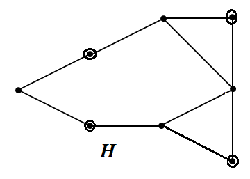
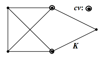
Figure 3: In graph $H,$ the number of vertices in CV and in NCV are the same and in graph $K,$ $|CV|<|N(CV)|$.

The relative number of vertices in $CV$ and in $N(CV)$ may differ. For the graphs $H$ and $K$ of Figure 3 $|CV|=|N(CV)|$ and $|CV|<|N(CV)|,$ respectively. In Section 4, we see that graphs with $|CV|>|N(CV)|$ exist, a property satisfied by minimal configurations (defined in Definition 15).

Theorem 11.

Let $G$ be a singular core-labelled graph with independent core vertices. Then $\eta(G)=|CV|-\textup{rank}(\mathbf{Q})$.

Proof.

By the well known dimension theorem,
                  Dim(Domain$({\bf Q}{{}^{\intercal}}))=$ Dim(Ker$({\bf Q}{{}^{\intercal}}))+$ Dim(Im$({\bf Q}{{}^{\intercal}})).$

Now Dim(Domain$({\bf Q}{{}^{\intercal}}))=|CV|.$ By Lemma 9, Dim(Ker$({\bf Q}{{}^{\intercal}}))=\eta(G).$ Hence rank$({\bf Q})=$ rank$({\bf Q}^{\intercal})=|CV|-\eta(G).$ ∎

It is clear that for a singular core–labelled graph, if $|CV|<|N(CV)|,$ then the columns of the $|CV|\times|N(CV)|$ matrix ${\bf Q}$ are linearly dependent. For $|CV|=|N(CV)|,$ by Theorem 11, $\textup{rank}(\mathbf{Q})<|CV|$ and thus the $|N(CV)|$ columns of $\mathbf{Q}$ are linearly dependent. We shall now determine a necessary and sufficient condition for $\mathbf{Q}$ to have full column rank.

Theorem 12.

Let $G$ be a singular core–labelled graph. The matrix $\mathbf{Q}$ has linearly independent columns if and only if $\eta(G)=|CV|-|N(CV)|$.

Proof.

The matrix $\mathbf{Q}$ has full rank if and only if rank$({\bf Q})={\rm Dim}({\rm Im}({\bf Q}))=|N(CV)|.$ By Theorem 11, the necessary and sufficient condition for the matrix $\mathbf{Q}$ to have linearly independent columns is that $\eta(G)=|CV|-|N(CV)|$. ∎

Recall that the vertex set $V$ of a core–labelled graph is partitioned into $CV$, $N(CV)$ and $CFV_{R}.$ On deleting $N(CV)$ and $CV$ from a graph, the subgraph induced by $CFV_{R}$ remains.

Theorem 13.

The subgraph induced by $CFV_{R}$ for a core–labelled graph is non–singular.

Proof.

Using an adjacency matrix ${\bf A}$ of the form (1), we need to show that $\mathbf{My=0}$ if and only if $\mathbf{y=0}.$ For a core–labelling, all kernel vectors of $\textbf{A}(G)$ are of the form ${\bf z}=\left(\begin{array}[]{c}{\bf x}\\ {\bf 0}\\ {\bf 0}\end{array}\right).$

But ${\bf My=0}$ for some ${\bf y}\not={\bf 0}$ if and only if there exists ${\bf x}$ such that ${\bf A}\left(\begin{array}[]{c}{\bf x}\\ {\bf 0}\\ {\bf y}\end{array}\right)={\bf 0}.$ This contradicts the form of the kernel vector for a core–labelling. Hence no kernel vectors exist for ${\bf M}.$ ∎

Graphs with independent core vertices include the family of half cores. A half core is a bipartite graph with one partite set being the set $CV$ and the other partite set being $CFV$. In Section 5, we shall see that trees also have independent core vertices.

At this stage, the case for unicyclic graphs is worth mentioning. The coalescence of two graphs is obtained by identifying a vertex of one graph with a vertex of the other graph. If none of the two graphs is $K_{1}$, then this vertex becomes a cut vertex. Unicyclic graphs can be considered to be the coalescence of a cycle $C_{r}$ with $r$ trees (some or all of which may be the isolated vertex $P_{1}$), each tree $T_{v}$ coalesced with $C_{r}$ at a unique vertex $v$ of the cycle. If $r\not=4k,\ k\in{\mathbb{Z}}^{+},$ then the unicyclic graph has independent core vertices. Since the nullity of $C_{4}$ is 2, using Theorem 5, the following result is immediate.

Theorem 14.

Let $G$ be a unicyclic graph with cycle $C_{r}$ where $r=4k.$

1. If the vertex $v$ of at least one tree $T_{v}$ which is coalesced with the cycle is a core–forbidden vertex, then the unicyclic graph also has independent core vertices.

2. If the vertices $v$ of each tree $T_{v}$ which is coalesced with the cycle is a core vertex, then the unicyclic graph must have nullity at least 2.

4 Bipartite Minimal Configurations

In [3, 4, 6], the concept of minimal configurations (MCs) as admissible subgraphs, that go to construct a singular graph, is introduced. It is shown that there are $\eta$ MCs as subgraphs of a singular graph $G$ of nullity $\eta>0.$ A MC is a graph of nullity 1 and its adjacency matrix ${\bf A}$ satisfies ${\bf Ax}={\bf 0}$ where ${\bf x}\not={\bf 0}$ is the generator of the nullspace of the adjacency matrix ${\bf A}$ of $G$. The core vertices of a MC induce a subgraph termed the core $F$ with respect to ${\bf x}.$ Among singular graphs with core $F$ and kernel vector ${\bf x},$ a MC has the least number of vertices and there are no edges joining pairs of core–forbidden vertices. For instance, the path $P_{7}$ on 7 vertices is a MC with ${\bf x}=(1,0,-1,0,1,0,-1)^{\intercal}.$

Definition 15.

A minimal configuration (MC) is a singular graph on a vertex set $V$ which is either $K_{1}$ or if $|V|\geq 3$, then it has a core $F=G\left[CV\right]$ and periphery $\mathcal{P}=V\backslash CV$ satisfying the following conditions,

1. $\eta(G)=1$,

2. $\mathcal{P}=\emptyset$ or $\mathcal{P}$ induces a graph consisting of isolated vertices,

3. $\left|\mathcal{P}\right|+1=\eta\left(F\right)$.

Note that a MC $\Gamma$ is connected. To see this, suppose $\Gamma$ is the disjoint union $G_{1}\dot{\cup}G_{2}$ of the graphs $G_{1}$ and $G_{2},$ labelled so that the core vertices of $G_{1}$ are labelled first followed by its cfv, then the cv of $G_{2}$ followed by its cfv. There exists a nullspace vector $({\bf x}_{1},{\bf 0},{\bf x}_{2},{\bf 0}),$ of ${\bf A}$ with each entry of ${\bf x}_{1}$ and of ${\bf x}_{2}$ non-zero. Since $({\bf x}_{1},{\bf 0},{\bf 0},{\bf 0}),$ and $({\bf 0},{\bf 0},{\bf x}_{2},{\bf 0}),$ are conformal linearly independent vectors in the nullspace of ${\bf A},$ the nullity of $G$ is at least 2, a contradiction. For the nullity to be 1, it follows without loss of generality, that $\mathbf{x}_{2}={\bf 0}.$ But then all vertices in $G_{2}$ lie in the periphery and by definition of MC, they form an independent set. Hence $G_{2}$ consists of isolated vertices that add $|G_{2}|\ (>0)$ to the nullity of $G_{1}$, a contradiction. Hence $G$ must consist of one component only.

The $n$–vertex set of a bipartite graph $G(V_{1},V_{2},E)$ is partitioned into independent sets $V_{1}$ and $V_{2}$ and has edges in $E$ between vertices in $V_{1}$ and vertices in $V_{2}.$ If the vertices in $V_{1}$ are labelled first, then the adjacency matrix of $G$ is of the form

$$\mathbf{A}=\left(\begin{array}[]{c|c}\mathbf{0}&\mathbf{S}\\ \hline\cr\mathbf{S}^{\intercal}&\mathbf{0}\end{array}\right),$$ (2)

where the $|V_{1}|\times|V_{2}|$ matrix $\mathbf{S}$ describes the edges between $V_{1}$ and $V_{2}$. The nullity of ${\bf A}$ is $n-2\ {\rm rank}({\bf S}).$ We have proved the following result:

Proposition 16.

The nullity of the adjacency matrix of an $n$–vertex bipartite graph and $n$ are of the same parity.

In [12], the result in Proposition 16 is obtained for trees, a subclass of the bipartite graphs. In particular, a bipartite non-singular graph has an even number of vertices.

To explore bipartite MCs it is convenient to consider first a singular bipartite graph of nullity 1.

Proposition 17.

A singular bipartite graph of nullity 1 admits a core–labelling.

Proof.

Let $G({V}_{1},{V}_{2},{E})$ be a singular bipartite graph with partite sets ${V}_{1}$ and ${V}_{2}.$ We show that $CV\subseteq{V}_{1},$ without loss of generality.

Suppose $CV\subseteq{V}_{1}\cup{V}_{2}.$ Then there exists ${\bf x}=\left(\alpha_{1},...,\alpha_{|{V}_{1}|},\beta_{1},...,\beta_{|{V}_{2}|}\right)^{\intercal},$ $\ {\bf x}\not={\bf 0},$ where not all the $\alpha_{i}$ are zero and not all the $\beta_{j}$ are zero. Then ${\bf A}\left(\alpha_{1},...,\alpha_{|{V}_{1}|},0,...,0\right)^{\intercal}={\bf 0}$ and ${\bf A}\left(0,...,0,\beta_{1},...,\beta_{|{V}_{2}|}\right)^{\intercal}={\bf 0},$ showing that ${\bf A}$ has two linearly independent nullspace vectors. This contradicts that the nullity of a MC is 1.

Hence without loss of generality, $\beta_{j}=0,\ 1\leq j\leq|{V}_{2}|,$ showing that the core vertices lie in ${V}_{1}.$ Thus the $CV$ of a bipartite MC is necessarily an independent set, which is the condition for the existence of a core–labelling. ∎

Theorem 18.

Let $G$ be a bipartite graph, of nullity 1, on $n$ vertices with partite vertex sets $V_{1}$ and $V_{2}$. Then,

1. $n$ is odd

2. For $|V_{1}|>|V_{2}|$, $|V_{2}|=\dfrac{n-1}{2}$ and $|V_{1}|=|V_{2}|+1$

3. $CV\subseteq V_{1}.$

Proof.

Let the adjacency matrix of $G$ be as in (2).

1. Since $\text{rank}(\mathbf{A})=2\,\text{rank}(\mathbf{S})$ and $\eta(G)=1$, then $n=2\,\text{rank}(\mathbf{S})+1$, which is odd.

2. Without loss of generality, let $|V_{1}|>|V_{2}|$. Then $\text{rank}(\mathbf{S})\leq|V_{2}|$. Hence $n-1=\text{rank}(\mathbf{A})\leq 2|V_{2}|.$ Thus $|V_{1}|+|V_{2}|-1\leq 2|V_{2}|$ and$|V_{1}|=|V_{2}|+1$. Since $n=|V_{1}|+|V_{2}|$, it follows that $|V_{2}|=\dfrac{n-1}{2}$.

3. The proof of Proposition 17 shows that $CV\subseteq{V}_{1}.$

∎

A MC has nullity equal to 1. For a bipartite MC, with partite sets $V_{1}$ and $V_{2},$ and $|V_{1}|>|V_{2}|,$ we have $|V_{1}|=|V_{2}|+1.$

Corollary 19.

Let $G$ be a bipartite MC with vertex partite sets $V_{1}$ and $V_{2},$ where $|V_{1}|>|V_{2}|.$ Then the set $CV$ of core vertices is $V_{1}$ and the set $CFV$ ( that is $\mathcal{P}$) is $V_{2}$.

Proof.

By Theorem 18(iii), $CV\subseteq{V}_{1}.$ A minimal configuration is connected and $V_{1}$ is an independent set in a bipartite MC. Note that $\mathcal{P}$ is an independent set. Thus the only neighbouring vertices of a vertex in $\mathcal{P}$ are in $CV.$ Since $\mathcal{P}=V\backslash CV,$ then $\mathcal{P}\cap V_{1}=\emptyset.$ Thus $\mathcal{P}\subseteq V_{2}$. Moreover $CV=V_{1}$ and $\mathcal{P}=V_{2}.$ ∎

Another characterization of a bipartite MC focuses on the removal of extra vertices and edges, from a singular bipartite graph of nullity 1, producing a slim graph (Definition 8, page 8).

Theorem 20.

A graph $G(V_{1},V_{2},E),$   $|V_{1}|>|V_{2}|,$ is a bipartite MC if and only if it is a slim bipartite graph of nullity 1 with $CV=V_{1}$.

Proof.

Let $G(V_{1},V_{2},E)$ be a bipartite MC, $|V_{1}|>|V_{2}|$. Then it has nullity 1 and $|V_{2}|=|V_{1}|-1$. The set $V_{1}$ is $CV$ and $V_{2}$ is $CFV={\mathcal{P}}.$ Thus it has no $CFV_{R}$ and is therefore a slim graph of nullity 1.

Conversely, let $G(V_{1},V_{2},E)$ be a slim bipartite graph of nullity 1, with $CV=V_{1}$. Then $V_{2}=CFV$ and by Theorem 18 (ii), $|V_{2}|=|V_{1}|-1.$ Removal of $V_{2}$ leaves the core $F,$ induced by $CV,$ with nullity $|CV|$ increasing the nullity from 1 to $|V_{1}|.$ But then the nullity increases by one with the removal of each vertex in $V_{2}.$ Thus $\mathcal{P}=V_{2}$ and is an independent set. Also $\eta(F)=|V_{1}|.$ Moreover $|\mathcal{P}|=|V_{2}|=\eta(F)-1.$ Hence $G$ is a bipartite MC. ∎

It is worth mentioning that stipulating that a MC is bipartite can do away with the third axiom of a general MC.

5 Nullspace Vertex Partition in Trees

Trees are the most commonly studied class of graphs [22]. In this section we explore MC trees and singular trees in general. First we need a result on the number of core vertices adjacent to any vertex of a singular graph on more than 1 vertex.

Lemma 21.

A vertex of a singular graph cannot be adjacent to exactly one core vertex.

Proof.

A graph is singular if there exists ${\bf x}\in{\mathbb{R}}^{n},\ {\bf x}\not={\bf 0},$ such that ${\bf Ax}={\bf 0}.$ Let $v\in V(G).$ The $v$th row of ${\bf Ax}={\bf 0}$ can be written as $\sum_{i\sim v}x_{i}=0.$ The neighbours of $v$ may be all $cfv$. If not, then there exists $w\in CV$ such that $w\sim v$ and $x_{w}\not=0.$ But then there exists at least one other $cv\ w^{\prime},\ w^{\prime}\sim v$ with $x_{w^{\prime}}\not=0$ to satisfy $\sum_{i\sim v}x_{i}=0.$ ∎

As a result of Lemma 21, if 2 core vertices are adjacent then an infinite path is a subgraph of a finite tree, since a tree has no cycles. This contradiction proves the following result

Proposition 22.

[10, 16] Let $T$ be a singular tree. Then $T$ has independent core vertices.

For a tree, the combinatorial properties of the subgraph induced by $CFV_{R}$ will prove useful in Theorem 28.

Theorem 23.

For a core–labelling of a singular tree $T,$ the subgraph induced by $CFV_{R}$ has a perfect matching.

Proof.

In Proposition 13, we show that $M$ as in (1) is invertible. The nullity $\eta(T)=n-2t=0.$ Hence the subgraph induced by $CFV_{R}$ has a perfect matching (a one–factor). ∎

We shall now use the concept of subdivision for the proof of the characterization of a MC tree.

Definition 24.

A subdivision $S$ of a connected graph $G$ on $n$ vertices and $m$ edges is obtained from $G$ by inserting a vertex of degree 2 in each edge. Thus $S$ has $n+m$ vertices and $2m$ edges.

Lemma 25.

Let ${\bf B}$ be the vertex–edge incidence matrix of a connected graph $G.$ The characteristic polynomial of the subdivision $S$ of a connected graph $G$ is $\phi(S,\lambda)=\lambda^{n-m}\det(\lambda^{2}{\bf I}-{\bf B}^{\intercal}{\bf B}).$

Proof.

The adjacency matrix of $S$ is

$${\bf A}(S)=\left(\begin{array}[]{c|c}{\bf 0}_{n}&{\bf B}\\ \hline\cr{\bf B}^{\intercal}&{\bf 0}_{m}\end{array}\right).$$ (3)

Expanding using Schur’s complement, $\phi(S,\lambda)=\lambda^{n}\det(\lambda{\bf I}-{\bf B}^{\intercal}(\lambda{\bf I})^{-1}{\bf B})=\lambda^{n-m}\det(\lambda^{2}{\bf I}-{\bf B}^{\intercal}{\bf B}).$ ∎

Corollary 26.

For a tree $T,$ the incidence matrix ${\bf B}$ has full rank.

Proof.

Consider ${\bf B}^{\intercal}\left(\begin{array}[]{c}\alpha_{1}\\ \alpha_{2}\\ \vdots\\ \alpha_{n}\end{array}\right)=\left(\begin{array}[]{c}0\\ 0\\ \vdots\\ 0\end{array}\right).$ Since there are only 2 non–zero entries in each column of ${\bf B},$  $\alpha_{u}=-\alpha_{w}$ for edge $\{u,w\}.$ For a connected graph, it follows that the nullspace of ${\bf B}^{\intercal}$ has dimension 1 for a bipartite graph and 0 otherwise. The tree $T$ is bipartite and $m=n-1.$ Hence the rank of ${\bf B}$ which is the same as the rank of ${\bf B}^{\intercal}$ is $m.$ ∎

Corollary 27.

The subdivision of a tree is singular with nullity 1.

Proof.

This follows immediately from Lemma 25 since from Corollary 26, the nullspace of ${\bf B}^{\intercal}{\bf B}$ is $\{\bf 0\}$ for a tree with $m=n-1.$ ∎

In [23], a characterization of MC trees is presented. Here we give a different proof by using Corollary 27.

Theorem 28.

[23] A tree is a minimal configuration if and only if it is a subdivision of another tree.

Proof.

Let $T^{\prime}$ be a MC with $|CV|=n$ and $|{\mathcal{P}}|=|N(CV)|=m.$ Then $m-n=1.$ Note that both $CV$ and $N(CV)$ are independent sets, the partite sets of $T^{\prime}.$ Also the number of edges of $T^{\prime}$ is $m+n-1=2m.$ Now a vertex of ${\mathcal{P}}(T^{\prime})$ cannot be an end vertex as otherwise its neighbour is a $cfv$, contradicting the independence of ${\mathcal{P}}(T^{\prime})$ in a MC. Thus each vertex of ${\mathcal{P}}(T^{\prime})$ has degree 2. Therefore $T^{\prime}$ is the subdivision of a tree $T$ on $n$ vertices and $m$ edges.

Conversely, let $T$ be a tree on $n$ vertices and $m$ edges and let $S$ be its subdivision. Then by Corollary 27, $S$ has nullity 1.

Since $S$ is a singular tree, then by Proposition 22, CV is an independent set. Hence $S$ has a core–labelling. Let the partite sets $V_{1}$ and $V_{2}$ in $S$ be the original vertices of $T$ and the inserted vertices, respectively. Note $|V_{1}|=|V_{2}|+1.$ By Theorem 18 (iii), $CV\subseteq V_{1}.$ Since $S$ is bipartite, $N(CV)\subseteq V_{2}.$

Recall that $V_{1}$ in $S$ was the set of original vertices of $T.$ Let $w\in V_{1}.$ The subgraph $S-w$ of $S,$ obtained from $S$ after removing $w$ has a perfect matching with edges $\{u_{i},w_{j}\},\ u_{i}\in V_{2},\ w_{j}\in V_{1}.$ Hence $S-w$ has nullity 0. This means that the nullity of $S$ decreases on deleting $w.$ Hence $w\in CV,$ that is $V_{1}\subseteq CV.$ The subset $V_{1}$ is therefore $CV$ in $S.$

We now consider $V_{2},$ which is a partition of $N(CV)$ and $CFV_{R}.$ Since the $S$ is connected, then $V_{2}=N(CV).$ It follows that $S$ is a bipartite slim graph of nullity 1, with $V_{1}=CV$. By Theorem 20, $S$ is a bipartite $MC$.

∎

Note that the subgraph of $S,$ obtained after removing $u\in V_{2},$ is a subdivision of a forest of two trees and has nullity 2. Repeating the process until all the vertices in $V_{2}$ are removed, the nullity increases to $V_{1}.$ Hence the nullity increased by 1 with each vertex deletion. It follows that each vertex in $V_{2}$ is an upper $cfv,$ a condition required for a MC. It is also worth noting that the incidence matrix $\bf B$ appearing as a submatrix of the adjacency matrix of a subdivision of a tree in (3) is precisely ${\bf Q}$ in (1).

We now show that the size of the periphery of a MC tree is related to the matching number $t.$

For a general singular tree $T$, a maximal matching consists of the pendant edges removed, until $\overline{K_{\eta(T)}}$ is obtained, starting from any end–vertex in $T.$ One can start from a slim forest and extend to a general tree $T^{\prime}$ of the same nullity with the CV preserved by adding pairs of adjacent vertices in $CFV_{R}(T^{\prime}).$ This can be done either by adding a pendant edge and joining it to a $cfv$ or by inserting two vertices of degree 2 in an edge with $cfv$s as end vertices.

Proposition 29.

If $T^{\prime}$ is a minimal configuration tree, then $t=|N(CV)|$.

Proof.

For a MC tree, $\eta(T^{\prime})=1=n(T^{\prime})-2t.$ Also, by Theorem 28, $T^{\prime}$ is the subdivision of a tree $T$ on $n$ vertices and $m$ edges. So $n(T^{\prime})=n+m$ and $2t=n+m-1=2m.$ Since the vertices in $N(CV(T^{\prime}))\ (={\mathcal{P}}(T^{\prime}))$ are the vertices inserted in the edges of $T$ to form the subdivision, $t=m=|N(CV)|$. ∎

The next result is on the rank of ${\bf Q}$ in the adjacency matrix of a core–labelled tree.

Theorem 30.

If $T$ is a core–labelled tree, then the columns of $\mathbf{Q}$ are linearly independent.

Proof.

For a core–labelled graph $G$, by Theorems 11, $\eta(G)=|CV|-\textup{rank}(\mathbf{Q})$. For a tree, $\eta(T)=n-2t.$ By Theorem 23, for a core–labelled tree, $2t=2|N(CV)|+|CFV_{R}|.$ Since $n=|CV|+|N(CV)|+|CFV_{R}|$, by eliminating t, $\eta(T)=|CV|-|N(CV)|$. By Theorem 12, $\mathbf{Q}$ has full rank and the $|N(CV)|$ columns of $\mathbf{Q}$ are linearly independent.

∎

6 Nullspace Preserving Edge Additions

In this last section, we explore which edges could be added (or removed) from a graph to preserve the nullity or the core vertex set.

By Cauchy’s Interlacing Theorem for real symmetric matrices, the nullity changes by at most 1, on adding or deleting a vertex. By definition, if the vertex is a $cfv_{mid},$ the nullity is preserved. We now explore which edge additions allow the nullity and the core vertex set to be both preserved in a graph with independent core–vertices. We use again the vertex partition into $CV$, $N(CV)$ and $CFV_{R}$ induced by a core–labelling. We consider adding an edge between two vertices within a part or between two distinct parts of the partition.

Theorem 31.

Let $G$ be a core-labelled graph. Let $u\in CV$ and $w\in N(CV)$, such that $u\nsim w$ in $G$. Let $G^{\prime}\coloneqq G+e$ be obtained from $G$ by adding an edge $e$ such that the core-labelling is preserved, where $e\coloneqq\{u,w\}$. Then $\eta(G^{\prime})\geq\eta(G).$ Moreover, there is a vector $\mathbf{x}_{{}_{CV}}$ which is in $\text{\rm Ker}\left(\mathbf{Q}^{\intercal}\right)$ but not in $\text{\rm Ker}\left(\left(\mathbf{Q^{\prime}}\right)^{\intercal}\right)$ and a vector $\mathbf{y}_{{}_{CV}}$ which is in $\text{\rm Ker}\left(\left(\mathbf{Q^{\prime}}\right)^{\intercal}\right)$ but not in $\text{\rm Ker}\left(\mathbf{Q}^{\intercal}\right)$ .

Proof.

For a core labelling of a graph $G,$ with vertices $u\in CV$ and $w\in N(CV)$ labelled 1 and $|CV|+1,$ respectively, such that $u\nsim w$ in $G,$ we write $u=1$ and $w=|CV|+1.$ Let the adjacency matrix $\mathbf{A}$ be as in (1). On adding edge $\{u,w\},$ the adjacency matrix $\mathbf{A}^{\prime}$ of $G^{\prime}$ satisfies $\mathbf{A}^{\prime}=\mathbf{A}+\mathbf{E}$ where

$$\mathbf{E}=\left(\begin{array}[]{c|c|c}0&1\ 0\ ...&0\\ \vspace*{-.35cm}\hfil&&\\ {\bf 0}&{\bf 0}&{\bf 0}\\ \hline\cr 1\ 0\ ...&\ 0\ ...&0\\ \vspace*{-.35cm}\hfil&&\\ {\bf 0}&{\bf 0}&{\bf 0}\\ \hline\cr{\bf 0}&{\bf 0}&{\bf 0}\\ \end{array}\right).$$

Since $u$ is a cv, there exists $\mathbf{x}^{(1)}$ in the nullspace of $\mathbf{A}$ with the first entry $\alpha$ non-zero. If $\eta(G)>1,$ let $\mathbf{x}^{(1)},\mathbf{x}^{(2)},...,\mathbf{x}^{\left(\eta(G)\right)}$ be a basis for the nullspace of $G$, such that only $\mathbf{x}^{(1)}$ has the first entry non-zero. Denoting column $i$ of the identity matrix by $\mathbf{e}_{i}$ and writing $\mathbf{x}^{(1)}=\left(\begin{array}[]{c}\mathbf{x}_{{}_{CV}}\\ \hline\cr{\bf 0}\\ \hline\cr{\bf 0}\end{array}\right),$ conformal with (1), row $w$ of $\mathbf{A}^{\prime}\mathbf{x}^{(1)}$ is $\mathbf{e}_{w}^{\intercal}(\mathbf{Q}^{\prime})^{\intercal}\mathbf{x}_{{}_{CV}}=\mathbf{e}_{w}^{\intercal}\mathbf{Q}^{\intercal}\mathbf{x}_{{}_{CV}}+\alpha=\alpha\neq{0}.$

Hence $\mathbf{Q}^{\prime}\mathbf{x}^{(1)}_{{}_{CV}}\neq{\bf 0}.$ By the proof of Lemma 9, $\mathbf{A}^{\prime}\mathbf{x}^{(1)}\neq{\bf 0}.$ Thus $\mathbf{x}^{(1)}$ is a vector in the nullspace of $\mathbf{A}$ but not in the nullspace of $\mathbf{A}^{\prime}.$ Moreover, $\left(\mathbf{Q^{\prime}}\right)^{\intercal}\mathbf{x}^{(i)}_{{}_{CV}}=\mathbf{0}$, for $2\leq i\leq\eta(G)$. Thus the $\eta(G)-1$ vectors $\mathbf{x}^{(2)},...,\mathbf{x}^{\left(\eta(G)\right)}$ lie in the nullspace of $G^{\prime}$.

Since $CV$ is preserved of adding edge $\{u,w\}$, $u$ is also a core vertex in $G^{\prime}$. Hence there is another vector $\mathbf{y}^{(1)}$ in the nullspace in $\mathbf{A}^{\prime}$ with the first entry non-zero. Therefore $\eta(G^{\prime})\geq\eta(G)$.

A similar argument as above yields $\eta(G^{\prime})\leq\eta(G)$, so that the graphs $G$ and $G^{\prime}$ have the same nullity. Moreover, $\mathbf{x}^{(1)}$ is a vector in the nullspace of $\mathbf{A}$ but not in the nullspace of $\mathbf{A}^{\prime}$ whereas $\mathbf{y}^{(1)}$ is a vector in the nullspace of $\mathbf{A}^{\prime}$ but not in the nullspace of $\mathbf{A}.$ ∎

As a consequence of Theorem 31, addition of an edge from a vertex in $CV$ to a vertex in $N(CV)$ which preserves the core-labelling does not change the nullity but may change the nullspace. The addition of edges between two vertices in $CV$ vertices is not possible as the core-labelling will not remain well defined. Furthermore, the addition of an edge between a $CV$ vertex and a $CFV_{R}$ vertex is not permissible either as the core-labelling changes.

Therefore, to preserve the core–labelling, only the following edge additions are left to be considered:

1. $N(CV)$ – $N(CV)$ edges,

2. $N(CV)$ – $CFV_{R}$ edges,

3. $CFV_{R}$ – $CFV_{R}$ edges.

Before presenting results on the perturbations that satisfy constraints relating to the nullspace of ${\bf A},$ we give examples to show the possible effects on the vertex types and on the nullspace on adding an edge to graphs with independent core vertices.

Figure 4: Adding edge $e=\{5,8\}$ to the tree $T$ of nullity 1 preserving the nullity but altering the core–vertex set.

Figure 4 shows tree $T$ and the unicyclic graph $T+e_{\{5,8\}}$ with core vertices $\{1,8\}$ replaced by $\{1,8,9\}.$ Figure 5 shows the half cores $H$ of nullity 2 and $H+e_{3,14}$ with the same core vertices but with different nullspace vectors of their adjacency matrix. The nullspace of ${\bf A}(H)$ is generated by

$$\{\{0,-1,0,0,0,1,0,-1,0,1,0,-1,0,1\},\{0,-1,0,-1,0,1,2,0,0,0,0,0,0,0\}\}$$

and on adding the edge $\{3,14\}$ the nullspace generator of ${\bf A}(H+e_{\{3,14\}})$ becomes

$$\{\{0,-1,0,1,0,1,0,-2,0,2,0,-2,0,2\},\{0,-1,0,-1,0,1,2,0,0,0,0,0,0,0\}\}.$$

Figure 5: Adding edge $e=\{3,14\}$ to the graph $H$ of nullity 2 preserving the nullity and the core–vertex set but altering the nullspace.

We give another example where the nullity changes from 0 to 2 on adding an edge. The perturbation to the tree $T^{\prime}$ shown in Figure 6 is the addition of edge $\{1,2\}$. The nullspace of ${\bf A}(T^{\prime})$ is generated by $\{0\}$ and on adding the edge $\{1,2\}$ the nullspace generator of ${\bf A}(T^{\prime}+e_{1,2})$ becomes $\{\{0,1,0,-1,0,1\},\{-1,0,1,0,0,0\}\}.$

Figure 6: Adding edge $e=\{1,2\}$ to the non–singular tree $T^{\prime}$ increases the nullity to 2 and creates a four core–vertex set.

Proposition 32.

Let $G$ be a graph with independent core vertices. Let $u$ and $w$ be core-forbidden vertices, such that $u\nsim w$ in $G$. Let $G^{\prime}\coloneqq G+e$ be obtained from $G$ by adding the edge $e=\{u,w\}$. If the nullity is preserved, then $G+e$ has the same nullspace and core-labelling of $G$.

Proof.

Let $G$ be labelled so that $\mathbf{A}$ is a block matrix as in (1). We show that a kernel vector $\mathbf{x}$ of $\mathbf{A}(G)$ is a kernel vector for $\mathbf{A}(G^{\prime})$.

Let $\mathbf{x}_{{}_{CV}}$ be the restriction $\left(\alpha_{1},\ldots,\alpha_{|CV|}\right)^{\intercal}$ of $\mathbf{x}$ to the core vertices of $G$. Then $\mathbf{x}=(\mathbf{x}_{{}_{CV}},{\bf 0}).$ By definition of a kernel vector, $\mathbf{A}(G)\mathbf{x}=\mathbf{0}$. Therefore $\mathbf{Q}^{\intercal}\mathbf{x}_{{}_{CV}}=\mathbf{0}.$

Now, on adding edge $e,$ the change in $\mathbf{A}(G)$ is contained in the blocks associated with the core-forbidden vertices. Therefore, $\mathbf{A}(G^{\prime})\mathbf{x}=\mathbf{Q}^{\intercal}\mathbf{x}_{CV}=\mathbf{0}.$

Therefore the kernel vectors of $\mathbf{A}(G)$ are also kernel vectors of $\mathbf{A}\left(G^{\prime}\right)$. Thus $CV(G)\subseteq CV\left(G^{\prime}\right)$, that is $\eta(G)\leq\eta\left(G^{\prime}\right)$. If a cfv in $G$ becomes a cv in $G^{\prime}$, then the nullity increases. But the nullity is preserved. Hence $CV$ is preserved and so is the nullspace. In turn, it follows that $N(CV)$ and core-labelling of $G$ are unaltered by the perturbation. ∎

The necessary condition established in Proposition 32 can be relaxed to a necessary and sufficient condition involving $CV$ only.

Theorem 33.

Let $G$ be a graph with independent core vertices. Let $u$ and $w$ be core-forbidden vertices, such that $u\nsim w$ in $G$. Let $G+e$ be an edge addition to $G$, where $e=\{u,w\}$. Then, nullity is preserved if and only if $CV(G)=CV(G+e)$.

Proof.

Let the nullity be preserved. By Proposition 32, it follows that the core-labelling is preserved and hence $CV(G)=CV(G+e)$.

Conversely, let $CV(G)=CV(G+e)$. Since the added edge is amongst the core-forbidden vertices in $G$, then $\mathbf{Q}(G)=\mathbf{Q}(G+e)$. By Theorem 11,

$$\eta(G) =|CV(G)|-\text{rank}(\mathbf{Q}(G))$$

$$=|CV(G+e)|-\text{rank}(\mathbf{Q}(G+e))$$

$$=\eta(G+e)$$

and hence nullity is preserved. ∎

The study of perturbations to networks finds many applications, in information technology and social networks in particular [17, 18, 19]. The results presented here are of interest in combinatorial optimization and the study of perturbations to singular networks with the goal of inserting or removing edges efficiently while maintaining the same core vertex set. In machine learning, to train a neural network, switches linked to edge detectors in the neural network stochastically disable specific detectors in accordance with a preconfigured probability. This technique is used to reduce over–fitting on the training data [20]. The behaviour of graph invariants, when applying changes to a graph with constraints associated with the nullspace of the adjacency matrix, leads to optimal architectures with a specified nullity, retaining the independence of the core vertex set or the core–labelling.

Many algorithms in predictive modelling depend on the processing of network graphs with underlying spanning trees in a network. The combinatorial properties of trees that we discussed shed light on their inherent structure and help to devise efficient algorithms. In the search for optimal network graphs with a constraint related to the nullspace of the adjacency matrix, one may start with a slim graph and add an admissible edge joining non–adjacent vertices. The goal can be the preservation of one or more of the three properties associated with the nullspace of the adjacency matrix. These are the nullity, the core–vertex set and the entries of the normalized basis vectors of the nullspace of the adjacency matrix.

Depending on the property to be preserved, edges can be added selectively to obtain optimal networks with a maximal number of edges having the constant property. We have shown that adding edges to a graph may alter the core vertex set, the nullity or the nullspace. Constraints may be imposed to keep one aspect unchanged. Theorem 31 shows that adding edges between the mixed types $CV$ and $N(CV)$ of vertices, while the core–labelling is unchanged, preserves the nullity but upsets the nullspace. By Theorem 33, adding edges between core–forbidden vertices is a safe operation since the core vertex set is left intact, as long as the nullity is unaltered.

References

- [1]
- [2] I. Gutman and I. Sciriha. Graphs with Maximum Singularity. Graph Theory Notes NewYork, 30:17–20, 1996.
- [3] I. Sciriha. On the coefficient of in the characteristic polynomial of singular graphs. Util. Math., 52:97–111, 1997.
- [4] I. Sciriha. On the construction of graphs of nullity one. Discrete Math., 181(1-3):193–211, 1998.
- [5] I. Sciriha. On the rank of graphs. In Y. Alavi, D.R. Lick, A. Schwenk, Combinatorics, Graph Theory and Algorithms, vol. II, New Issue Press, Western Michigan University, Kalamazoo, Michigan, 769–778, 1999.
- [6] I. Sciriha. A characterization of singular graphs. Electron. J. Linear Algebra, 16:451–462 (electronic), 2007.
- [7] I. Sciriha. Coalesced and Embedded Nut Graphs in Singular Graphs. Ars Mathematica Contemporanea, 1:20–31 (http://amc.imfm.si), 2008.
- [8] I. Sciriha and A. Farrugia. From nutgraphs to molecular structure and conductivity. Mathematical Chemistry Monographs, University of Kragujevac, Series Eds. I. Gutman and B. Furtula, 2020.
- [9] V.E.Levit and E. Mandrescu. Combinatorial properties of the family of maximum stable sets of a graph. Discret. Appl. Math. 117: 149–161, 2002.
- [10] A. Neumaier. The second largest eigenvalue of a tree. Linear Algebra Appl. 46:9–25, 1982.
- [11] S.C. Gong and G.H. Xu. On the nullity of a graph with cutpoints. Linear Algebra and its Applications, 436:1, 135–142, 2012
- [12] J.H. Bevis, G.S. Domke, and V.A. Miller. Ranks of trees and grid graphs. J. of Combinatorial Math. and Combinatorial Computing, 18:109–119, 1995.
- [13] A. J. Schwenk. On the eigenvalues of a graph. In L.W. Beineke and R. J.Wilson, editors, Selected Topics in Graph Theory, chapter 11, pages 307–336. Academic Press, 1978.
- [14] T. Sander and J.W. Sander. Tree decomposition by eigenvectors. Linear Algebra and its Applications, 430(1):133 – 144, 2009.
- [15] I. Sciriha. Maximal and extremal singular graphs. Sovremennaya Matematika i Ee Prilozheniya-Contemporary Mathematics and its Applications, 71:1–9, 2011. Journal of Mathematical Sciences, 182:2, 2012.
- [16] D. A. Jaume and G. Molina. Null decomposition of trees. Discrete Mathematics, 341(3):836 – 850, 2018.
- [17] Y. Wang and Y. Z. Fan. The least eigenvalue of signless laplacian of graphs under perturbation. Linear Algebra and its Applications, 436(7):2084 – 2092, 2012.
- [18] R. Rowlinson. More on graph perturbations. Bull. London Math. Soc., pages 209–216, 1990.
- [19] I. Sciriha and J. Briffa. On the displacement of eigenvalues when removing a twin vertex. Discussiones Mathematicae (in press), arXiv preprint arXiv:1904.05670, 2019.
- [20] G. E. Hinton, A. KrizhevskyIlya, and S. Srivastva. System and method for addressing overfitting in a neural network patent, 0347558 A1, https://patents.google.com/patent/US9406017B2/en, 2019.
- [21] I. Gutman and D. M. Cvetković. The algebraic multiplicity of the number zero in the spectrum of a bipartite graph. Matematički Vesnik, 9(24)(56):141–150, 1972.
- [22] S. Fiorini, I. Gutman, and I. Sciriha. Trees with maximum nullity. Linear Algebra Appl., 397:245–251, 2005.
- [23] I. Sciriha and I. Gutman. Minimal configuration trees. Linear Multilinear Algebra, 54(2):141–145, 2006.