Anomalous Josephson Hall effect charge and transverse spin currents
in superconductor/ferromagnetic insulator/superconductor junctions

Abstract

Interfacial spin-orbit coupling in Josephson junctions offers an intriguing way to combine anomalous Hall and Josephson physics in a single device. We study theoretically how the superposition of both effects impacts superconductor/ferromagnetic insulator/superconductor junctions’ transport properties. Transverse momentum-dependent skew tunneling of Cooper pairs through the spin-active ferromagnetic insulator interface creates sizable transverse Hall supercurrents, to which we refer as anomalous Josephson Hall effect currents. We generalize the Furusaki–Tsukada formula, which got initially established to quantify usual (tunneling) Josephson current flows, to evaluate the transverse current components and demonstrate that their amplitudes are widely adjustable by means of the spin-orbit coupling strengths or the superconducting phase difference across the junction. As a clear spectroscopic fingerprint of Josephson junctions, well-localized subgap bound states form around the interface. By analyzing the spectral properties of these states, we unravel an unambiguous correlation between spin-orbit coupling-induced asymmetries in their energies and the transverse current response, founding the currents’ microscopic origin. Moreover, skew tunneling simultaneously acts like a transverse spin filter for spin-triplet Cooper pairs and complements the discussed charge current phenomena by their spin current counterparts. The junctions’ universal spin–charge current cross ratios provide valuable possibilities to experimentally detect and characterize interfacial spin-orbit coupling.

I Introduction

Superconducting junctions offer unique possibilities to generate and control charge and spin supercurrents, and provide the key ingredients for spintronics applications Eschrig (2011); Linder and Robinson (2015). Particularly rich physics occurs when superconductivity is brought together with the antagonistic ferromagnetic phase. Prominent examples cover magnetic Josephson junctions Bulaevskii et al. (1977a); *Bulaevskii1977alt; Buzdin et al. (1982a); *Buzdin1982alt; Andreev et al. (1991); Demler et al. (1997); Golubov et al. (2004); Buzdin (2005); Bergeret et al. (2005); Annunziata et al. (2011); Campagnano et al. (2015); Gingrich et al. (2016); Minutillo et al. (2018), in which the combination of superconductivity and ferromagnetism can add intrinsic phase shifts to the junctions’ characteristic current-phase relation and reverse the Josephson currents’ directions.

The interplay of magnetism and superconductivity gets even more fascinating in the presence of Rashba Bychkov and Rashba (1984) and/or Dresselhaus Dresselhaus (1955) spin-orbit coupling (SOC) Žutić et al. (2004); Fabian et al. (2007), which induces spin-triplet correlations Bergeret et al. (2001); Volkov et al. (2003); Keizer et al. (2006); Halterman et al. (2007); Eschrig and Löfwander (2008); Eschrig (2011); Sun and Shah (2015), triggers long-range proximity effects Duckheim and Brouwer (2011); Bergeret and Tokatly (2013, 2014); Jacobsen and Linder (2015), and is furthermore expected to host Majorana states in proximitized superconducting regions Nilsson et al. (2008); Duckheim and Brouwer (2011); Lee et al. (2012); Nadj-Perge et al. (2014); Dumitrescu et al. (2015); Pawlak et al. (2016); Ruby et al. (2017); Livanas et al. (2019). Tunneling barriers invariably introduce interfacial SOC into various types of (superconducting) tunnel junctions. Earlier theoretical studies concluded that skew tunneling of spin-polarized electrons through such barriers gives rise to (extrinsic) tunneling anomalous Hall effects (TAHEs) Vedyayev et al. (2013a, b); Matos-Abiague and Fabian (2015); Dang et al. (2015); Mironov and Buzdin (2017); Dang et al. (2018). Although first experiments carried out on granular nanojunctions Zhuravlev et al. (2018) essentially confirmed the theoretical expectations, the effect is typically weak in normal-state junctions. More sizable TAHE conductances, coming along with a spontaneous transverse supercurrent response, were predicted for superconducting junctions Costa et al. (2019), opening several novel perspectives, e.g., the possibility to experimentally verify superconducting magnetoelectric effects Edelstein (1995, 2003).

From that viewpoint, integrating TAHEs into Josephson junctions could likewise attract considerable interest. The resulting dissipationless transverse supercurrent flows might be efficiently tuned by means of the phase difference between the superconducting junction electrodes, becoming exploitable for a variety of spintronics applications Eschrig (2011); Linder and Robinson (2015). However, already one of the initial works into that direction Mal’shukov and Chu (2008) demonstrated that the fundamental time-reversal (electron–hole) symmetry in stationary Josephson junctions acts against the spontaneous flow of (spin) Hall supercurrents. To overcome this obstacle, one could either apply a finite bias voltage to the system Mal’shukov and Chu (2011) or modify the considered junction geometry. Several proposals suggested to focus on intricate magnetic multilayer configurations Asano (2005, 2006); Lu and Yip (2009); Mal’shukov et al. (2010); Brydon et al. (2011); *Brydon2012; Wang et al. (2011a, b); Bujnowski et al. (2012); Ren and Wang (2013); Alidoust and Halterman (2015); Wakamura et al. (2015); Yokoyama (2015); Bergeret and Tokatly (2016); Linder et al. (2017); Mironov and Buzdin (2017); Risinggård and Linder (2019), which break time-reversal symmetry and simultaneously facilitate a mixture of spin-singlet and spin-triplet correlations (caused, e.g., by strong SOC), eventually leading not only to nonzero charge Hall supercurrents Wang et al. (2011b); Yokoyama (2011, 2015); Mironov and Buzdin (2017), but also to their spin counterparts Lu and Yip (2009); Mal’shukov et al. (2010); Wang et al. (2011a); Ren and Wang (2013); Wakamura et al. (2015); Bergeret and Tokatly (2016); Linder et al. (2017); Ouassou et al. (2017); Risinggård and Linder (2019).

In this paper, we consider a ballistic superconductor (S)/ferromagnetic insulator (F-I)/S Josephson junction, whose magnetic (F-I) tunneling barrier introduces strong interfacial SOC into the system. We demonstrate that Cooper pairs skew tunnel through the spin-active interface and spontaneously generate charge Hall supercurrents along the transverse directions (i.e., parallel to the interface), to which we refer as anomalous Josephson Hall effect (AJHE) currents . When compared to most of the previously predicted geometries, our system brings along the great advantage that its physical properties can be much better controlled in experiments. Generalizing the Green’s function-based McMillan (1968) Furusaki–Tsukada method Furusaki and Tsukada (1991), we quantify the AJHE currents for representative junction parameters and discuss their characteristic dependence on the F-I’s magnetization orientation and the phase difference across the junction.

A clear spectroscopic fingerprint of Josephson junctions is the formation of subgap bound states, which are strongly localized around the nonsuperconducting link. In fact, two distinct types of bound states play a major role in S/F-I/S junctions Costa et al. (2018); Rouco et al. (2019): the Andreev bound states (ABS) Andreev (1964a); *Andreev1964alt; Andreev (1966a); *Andreev1966alt and the Yu–Shiba–Rusinov (YSR) Yu (1965); Shiba (1968); Shiba and Soda (1969); Rusinov (1968); *Rusinov1968alt states. Up to now, it remained unclear whether one can draw connections between these states’ features and the Josephson Hall effects. To answer this question, we identify our junction’s ABS and YSR states, together with their respective energies, and formulate an alternative approach that allows us to compute the AJHE currents directly from the bound state wave functions. The additional calculations offer not only an essential cross-check for the Furusaki–Tsukada method, but enable us to resolve the single current contributions that originate from the ABS and the YSR states. We identify SOC-induced transverse momentum-dependent asymmetries in the bound state energies, most clearly apparent in the YSR branch of the spectrum, as the microscopic origin of the AJHE.

The spin-active F-I barrier simultaneously induces interfacial spin flips and converts some of the spin-singlet Cooper pairs into triplet pairs. We extend the Cooper pair skew tunneling picture to these spin-polarized triplet pairs and develop a qualitative physical understanding to unravel the most essential features of the resulting transverse spin current flows. We evaluate the spin current amplitudes once from an extended Furusaki–Tsukada spin current formula and once from the bound state wave functions, comment on their distinct magnetization angle dependence when compared to their AJHE charge current counterparts, and eventually deduce that the magnetization-independent spin–charge current cross ratios could be exploited to classify the interfacial SOC.

We structured the paper in the following way. In Sec. II, we formulate the theoretical model used to investigate our junction. After working out the qualitative skew tunneling picture, justifying the existence of nonzero AJHE currents and bringing along valuable physical insight, in Sec. III, we compute the current components for realistic parameter configurations and discuss their generic properties (see Sec. IV). Section V is dedicated to a thorough analysis of the connections between the bound states that form around the junction’s F-I barrier and the emergent AJHE. Finally, we are concerned with the charge currents’ spin counterparts in Sec. VI, before closing with a short summary (Sec. VII). The Appendices contain the most important technical details of our calculations.

II Theoretical modeling

We consider a ballistic three-dimensional S/F-I/S junction grown along the $\hat{z}$-direction, in which the two semi-infinite S regions are separated by an ultrathin F-I (could, e.g., be a thin layer of $\mathrm{EuS}$ Moodera et al. (1988), $\mathrm{EuO}$ Tedrow et al. (1986), a $\mathrm{GaAs}$/$\mathrm{Fe}$ slab Hupfauer et al. (2015), or another thin semiconducting layer proximitized by a ferromagnet); see Fig. 1(a).

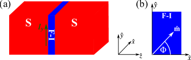
Figure 1: (a) Sketch of the regarded S/F-I/S junction, using the $C_{2v}$ principal crystallographic orientations $\hat{x}\parallel[110]$, $\hat{y}\parallel[\overline{1}10]$, and $\hat{z}\parallel[001]$; Cooper pair tunneling generates (tunneling) Josephson currents along $\hat{z}$, while the AJHE currents flow transversely along $\hat{x}$ and $\hat{y}$ ($I_{y}$ is exemplarily illustrated by the green arrow). (b) The direction of the magnetization vector inside the F-I, $\hat{\mathbf{m}}$, is determined by the angle $\Phi$.

The barrier itself introduces potential scattering and, owing to the broken space inversion symmetry, simultaneously additional strong interfacial Rashba Bychkov and Rashba (1984) and, for $C_{2v}$-symmetrical interfaces, Dresselhaus Dresselhaus (1955) SOC Žutić et al. (2004); Fabian et al. (2007). Our system is modeled by means of the stationary Bogoljubov–de Gennes (BdG) Hamiltonian De Gennes (1989),

$$\hat{\mathcal{H}}_{\mathrm{BdG}}=\left[\begin{matrix}\hat{\mathcal{H}}_{\mathrm{e}}&\hat{\Delta}_{\mathrm{S}}(z)\\ \hat{\Delta}_{\mathrm{S}}^{\dagger}(z)&\hat{\mathcal{H}}_{\mathrm{h}}\end{matrix}\right],$$ (1)

with $\hat{\mathcal{H}}_{\mathrm{e}}=[-\hbar^{2}/(2m)\,\bm{\nabla}^{2}-\mu]\,\hat{\sigma}_{0}+\hat{\mathcal{H}}_{\text{F-I}}$ representing the single-electron Hamiltonian and $\hat{\mathcal{H}}_{\mathrm{h}}=-\hat{\sigma}_{y}\,\hat{\mathcal{H}}_{\mathrm{e}}^{*}\,\hat{\sigma}_{y}$ its holelike counterpart ($\hat{\sigma}_{0}$ and $\hat{\sigma}_{i}$ indicate the two-by-two identity and the $i$th Pauli matrix). Analogously to previous studies de Jong and Beenakker (1995); Žutić and Valls (1999, 2000); Costa et al. (2017, 2018, 2019), the ultrathin F-I region is included into our model as an effective potential- and SOC-dependent deltalike barrier,

$$\hat{\mathcal{H}}_{\text{F-I}}=\Big{[}\lambda_{\mathrm{SC}}\,\hat{\sigma}_{0}+\lambda_{\mathrm{MA}}\,(\hat{\mathbf{m}}\cdot\hat{\bm{\sigma}})\\ +\alpha\,(k_{y}\,\hat{\sigma}_{x}-k_{x}\,\hat{\sigma}_{y})-\beta\,(k_{y}\,\hat{\sigma}_{x}+k_{x}\,\hat{\sigma}_{y})\Big{]}\,\delta(z),$$ (2)

where the first two parts describe scalar and magnetic tunneling with amplitudes $\lambda_{\mathrm{SC}}$ and $\lambda_{\mathrm{MA}}$, respectively. The unit vector along the magnetization direction in the F-I, $\hat{\mathbf{m}}=[\cos\Phi,\,\sin\Phi,\,0\big{]}^{\top}$, is determined with respect to the $\hat{x}\parallel[110]$-reference direction [see Fig. 1(b)], while the vector $\hat{\bm{\sigma}}=[\hat{\sigma}_{x},\,\hat{\sigma}_{y},\,\hat{\sigma}_{z}]^{\top}$ comprises the Pauli spin matrices. Finally, the remaining contributions resemble the interfacial Rashba and (linearized) Dresselhaus SOC with the effective strengths $\alpha$ in the first and $\beta$ in the second case; the SOC Hamiltonian is given with respect to the $C_{2v}$ principal crystallographic axes $\hat{x}\parallel[110]$ and $\hat{y}\parallel[\overline{1}10]$. Inside the S electrodes, the $s$-wave superconducting pairing potential, $\hat{\Delta}_{\mathrm{S}}(z)=|\Delta_{\mathrm{S}}|\,[\Theta(-z)+\mathrm{e}^{\mathrm{i}\phi_{\mathrm{S}}}\Theta(z)]$ ($|\Delta_{\mathrm{S}}|$ is the superconductors’ isotropic energy gap, which is taken to be the same in both electrodes, and $\phi_{\mathrm{S}}$ the phase difference across the junction) couples the BdG Hamiltonian’s electron and hole blocks. Writing $\hat{\Delta}_{\mathrm{S}}$ in that way is a rigid approximation as it fully neglects proximity effects. Nevertheless, this approach drastically simplifies the subsequent theoretical analyses, while still yielding reliable results for common transport calculations Likharev (1979); Beenakker (1997). For further simplification and without losing generality, we additionally consider equal effective carrier masses, $m$, and the same Fermi level, $\mu=(\hbar^{2}q_{\mathrm{F}}^{2})/(2m)$ ($q_{\mathrm{F}}$ is the associated Fermi wave vector), in all junction constituents.

Assuming translational invariance parallel to the F-I interface, the solutions of the BdG equation, $\hat{\mathcal{H}}_{\mathrm{BdG}}\,\Psi(\mathbf{r})=E\,\Psi(\mathbf{r})$, can be factorized into $\Psi(\mathbf{r})=\psi(z)\,\mathrm{e}^{\mathrm{i}(\mathbf{k_{\parallel}}\cdot\mathbf{r_{\parallel}})}$, where $\mathbf{k_{\parallel}}=[k_{x},\,k_{y},\,0]^{\top}$ ($\mathbf{r_{\parallel}}=[x,\,y,\,0]^{\top}$) is the transverse momentum (position) vector and $\psi(z)$ the BdG equation’s individual solution for the effective one-dimensional scattering problem along $\hat{z}$. The latter distinguishes between the involved quasiparticle scattering processes at the interface. Quasiparticles incident from one S may, for instance, either undergo Andreev reflection (AR) or specular reflection (SR), or may be transmitted into the second S. The AR process contains all the information concerning the transfer of Cooper pairs across the barrier and is therefore the process on which we need to focus subsequently to understand the physical origin of transverse supercurrent flows. Putting the scattering picture on a mathematical ground is rather technical and can be partly found in Appendix A and in all details in the Supplemental Material (SM) .

III Quasiparticle picture—Skew AR

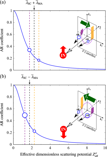
Figure 2: (a) Calculated (zero-energy) AR coefficient (determining the AR probability) for spin up electrons (IN) incident on the F-I interface and as a function of $Z_{\mathrm{eff}}^{\sigma}=(2mV_{\mathrm{eff}}^{\sigma})/(\hbar^{2}q_{\mathrm{F}})$, essentially modeling the effective scattering potential in Eq. (3). The dashed black line indicates the tunneling parameters $\overline{\lambda}_{\mathrm{SC}}=(2m\lambda_{\mathrm{SC}})/(\hbar^{2}q_{\mathrm{F}})=2$ and $\overline{\lambda}_{\mathrm{MA}}=(2m\lambda_{\mathrm{MA}})/(\hbar^{2}q_{\mathrm{F}})=0.25$, which combine to $\overline{\lambda}_{\mathrm{SC}}+\overline{\lambda}_{\mathrm{MA}}$ for up-spin electrons. Assuming the Rashba SOC strength $\overline{\lambda}_{\mathrm{R}}=(2m\alpha)/\hbar^{2}=1$, incoming electrons with $k_{y}>0$ are exposed to a raised (dashed orange line) and those with $k_{y}<0$ to a lowered (dashed violet line) effective scattering potential. AR becomes suppressed at positive $k_{y}$ and favorable at negative $k_{y}$, highlighted by the different size of the (blue) Andreev reflected holes. This skew AR generates a net transverse current along $\hat{y}$ (the direction of the current is usually defined oppositely to the electron flow direction; the latter points along $-\hat{y}$), which flows as a dissipationless AJHE current, $I_{y}$, in the superconductors. (b) Same as in (a), but for incident spin down electrons. Skew AR causes now an AJHE current along $-\hat{y}$. Since the effective tunneling strength (without SOC) for down-spin electrons is $\overline{\lambda}_{\mathrm{SC}}-\overline{\lambda}_{\mathrm{MA}}$, the skew AR coefficients for spin down are always slightly greater than for spin up so that the AJHE currents originating from both processes do not completely compensate.

On the quasiparticle level, the supercurrent generating exchange of Cooper pairs between the superconductors is mediated by the peculiar AR process. An (unpaired) electronlike quasiparticle incident on the F-I barrier from one S gets transmitted into the second S, pairs with another correlated electronlike quasiparticle, and effectively transfers a Cooper pair across the barrier. Formally, the transmission of two correlated electronlike quasiparticles is modeled by having the incident electronlike quasiparticle Andreev reflected as a holelike quasiparticle with opposite spin. As long as more Cooper pairs enter the right S than the left one (or vice versa), net (tunneling) Josephson currents start to flow. In the following, we will simply refer to electronlike (holelike) quasiparticles as electrons (holes). Electrons incident on the F-I barrier are exposed to an effective scattering potential that combines the scalar and (spin-dependent) magnetic potential terms with an additional transverse momentum- and spin-dependent contribution originating from the interfacial SOC. Assuming, for simplicity, that only Rashba SOC is present ($\alpha>0$ and $\beta=0$), the F-I’s magnetization points along $\hat{x}$ (meaning $\Phi=0$), and $k_{x}=0$, the effective scattering potential takes the form

$$V_{\mathrm{eff}}^{\sigma}=\lambda_{\mathrm{SC}}+\sigma\lambda_{\mathrm{MA}}+\sigma\alpha k_{y},$$ (3)

where $\sigma=+(-)1$ indicates a spin parallel (antiparallel) to $\hat{x}$; we will equivalently use the terms spin up (spin down). How does $V_{eff}^{\sigma}$ impact the peculiar AR process at the F-I barrier? To address this central question, Fig. 2 illustrates the dependence of the AR coefficient Note (2) on the strength of $V_{\mathrm{eff}}^{\sigma}$ [represented by the dimensionless parameter $Z_{\mathrm{eff}}^{\sigma}=(2mV_{\mathrm{eff}}^{\sigma})/(\hbar^{2}q_{\mathrm{F}})$]. We just focus on (spin-conserving) AR since this scattering process essentially drives the supercurrents we are predominantly interested in. Earlier studies Costa et al. (2019) showed that the contributions of spin-flip AR, i.e., the triplet Cooper pair currents are small within the considered limit and can be neglected when formulating a qualitative picture.

Following Eq. (3), incident up-spin electrons with $k_{y}>0$ experience a raised effective scattering potential, while $V_{\mathrm{eff}}^{\sigma}$ gets lowered for incoming $k_{y}<0$-electrons. Since the probability to undergo AR typically decreases with increasing $V_{\mathrm{eff}}^{\sigma}$, up-spin electrons get predominantly Andreev reflected for negative $k_{y}$. In that way, this skew AR generates a transverse AJHE quasiparticle current along the $\hat{y}$-direction. Although we are solely dealing with quasiparticle currents at the moment, skew AR effectively cycles Cooper pairs across the F-I interface and triggers a supercurrent response Costa et al. (2019). Therefore, the transverse AJHE quasiparticle currents building up at the interface are immediately converted into transverse AJHE supercurrents inside the two superconducting electrodes (basically generated by skew tunneling Cooper pairs). Flipping the incident electrons’ spin reverses the skew AR picture. It is now the positive range of $k_{y}$ that causes preferential ARs, leading to an AJHE current that flows along $-\hat{y}$. If the F-I barrier would be nonmagnetic, the net AJHE current amplitudes stemming from skew ARs of incoming up-spin and down-spin electrons would become equal and, as they flow along reversed directions, no net AJHE currents are expected. Already a weak exchange splitting in the F-I, however, is sufficient that skew ARs happen more likely for incoming down-spin than for up-spin electrons (see our explanations to Fig. 2). The individual AJHE currents in the (weakly) magnetic junction do then not completely cancel and nonzero AJHE currents build up.

IV AJHE currents

Measuring a finite AJHE supercurrent response is an unambiguous experimental evidence for skew ARs at the spin-active F-I interface. To mathematically access the interfacial AJHE currents in our junction (we refer to them as $I_{\eta}$ flowing along the $\hat{\eta}\in\{\hat{x};\hat{y}\}$-directions), we generalize the quasiparticle-based Furusaki–Tsukada approach Furusaki and Tsukada (1991) and end up with Note (2); Costa et al. (2019)

$$I_{\eta} \approx\frac{ek_{\mathrm{B}}T}{2\hbar}|\Delta_{\mathrm{S}}(0)|\tanh\left(1.74\sqrt{\frac{T_{\mathrm{C}}}{T}-1}\right)$$

$$\hskip 10.0pt\times\frac{A}{(2\pi)^{2}}\int\mathrm{d}^{2}\mathbf{k}_{\parallel}\sum_{\omega_{n}}\frac{k_{\eta}}{\sqrt{q_{\mathrm{F}}^{2}-\mathbf{k}_{\parallel}^{2}}}$$

$$\hskip 10.0pt\times\left[\frac{\mathcal{C}^{(1)}(\mathrm{i}\omega_{n})+\mathcal{D}^{(2)}(\mathrm{i}\omega_{n})+\mathcal{A}^{(3)}(\mathrm{i}\omega_{n})+\mathcal{B}^{(4)}(\mathrm{i}\omega_{n})}{\sqrt{\omega_{n}^{2}+|\Delta_{\mathrm{S}}(0)|^{2}\tanh^{2}\left(1.74\sqrt{T_{\mathrm{C}}/T-1}\right)}}\right],$$ (4)

where $e$ denotes the (positive) elementary charge, $k_{\mathrm{B}}$ Boltzmann’s constant, and $\omega_{n}=(2n+1)\pi k_{\mathrm{B}}T$, with integer $n$, indicates the fermionic Matsubara frequencies (at temperature $T$ and given in units of $1/\hbar$); for simplicity, we assume that the tunneling and Hall contact areas are equal and determined by $A$. All information necessary to evaluate the AJHE current components enters via the spin-conserving AR coefficients for incoming (from the left) up-spin (down-spin) electronlike quasiparticles, $\mathcal{C}^{(1)}(\mathrm{i}\omega_{n})$ [$\mathcal{D}^{(2)}(\mathrm{i}\omega_{n})$], as well as the ones belonging to incident up-spin (down-spin) holelike quasiparticles, $\mathcal{A}^{(3)}(\mathrm{i}\omega_{n})$ [$\mathcal{B}^{(4)}(\mathrm{i}\omega_{n})$]. The latter are required to properly capture the AJHE currents originating from skew ARs of electrons incident on the F-I interface from the right. Further details on the methodology are included into Appendix A and the SM Note (2).

In Fig. 3, we show the numerically extracted AJHE currents, $I_{x}$ and $I_{y}$, for one representative S/F-I/S junction.

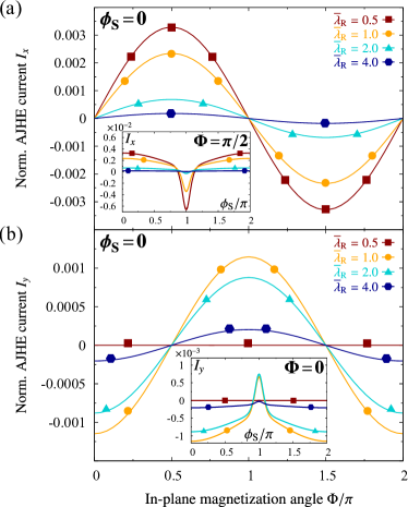
Figure 3: (a) Calculated dependence of the AJHE current along $\hat{x}$, $I_{x}$, normalized according to $(I_{x}e)/[G_{\mathrm{S}}\pi|\Delta_{\mathrm{S}}(0)|]$ [$e$ is the (positive) elementary charge and $G_{\mathrm{S}}$ represents Sharvin’s conductance of a three-dimensional point contact], on the F-I’s in-plane magnetization angle, $\Phi$, and for various indicated (dimensionless) Rashba SOC strengths, $\overline{\lambda}_{\mathrm{R}}=(2m\alpha)/\hbar^{2}$. The remaining parameters are $\overline{\lambda}_{\mathrm{SC}}=(2m\lambda_{\mathrm{SC}})/(\hbar^{2}q_{\mathrm{F}})=1$, $\overline{\lambda}_{\mathrm{MA}}=(2m\lambda_{\mathrm{MA}})/(\hbar^{2}q_{\mathrm{F}})=0.005$, and $\overline{\lambda}_{\mathrm{D}}=(2m\beta)/\hbar^{2}=0.5$. The temperature is chosen such that $T/T_{\mathrm{C}}=0.1$, where $T_{\mathrm{C}}\approx 16\,\mathrm{K}$ abbreviates the superconductors’ critical temperature. The inset shows the maximal $I_{x}$ (i.e., for $\Phi=\pi/2$) as a function of the superconducting phase difference, $\phi_{\mathrm{S}}$. (b) Similar calculations as in (a) for the AJHE current along $\hat{y}$, $I_{y}$.

For the superconducting materials’ zero-temperature gap and their critical temperature, we substituted realistic values for $s$-wave superconductors Carbotte (1990), $|\Delta_{\mathrm{S}}(0)|\approx 2.5\,\mathrm{meV}$ and $T_{\mathrm{C}}\approx 16\,\mathrm{K}$. The F-I parameters refer, e.g., to a weakly magnetic barrier (exchange couplings in the $\mathrm{meV}$-range) with a height of about $0.75\,\mathrm{eV}$ and a width of about $0.40\,\mathrm{nm}$ (assuming $q_{\mathrm{F}}\approx 8\times 10^{7}\,\mathrm{cm}^{-1}$ as a typical Fermi wave vector Martínez et al. (2020)); the chosen Dresselhaus SOC, $\overline{\lambda}_{\mathrm{D}}=(2m\beta)/\hbar^{2}=0.5$, corresponds to typical Dresselhaus SOC strengths of $\beta\approx 1.9\,\mathrm{eV}\,\text{\AA}^{2}$ (for example, $\mathrm{AlP}$ barriers with the considered height and width would have $\beta\approx 1.7\,\mathrm{eV}\,\text{\AA}^{2}$ Fabian et al. (2007); Note (2)), while the dimensionless Rashba measure got varied between $\overline{\lambda}_{\mathrm{R}}=(2m\alpha)/\hbar^{2}=0.5$ and $\overline{\lambda}_{\mathrm{R}}=4.0$, indicating bare Rashba SOC strengths between $\alpha\approx 1.9\,\mathrm{eV}\,\text{\AA}^{2}$ and $\alpha\approx 15.2\,\mathrm{eV}\,\text{\AA}^{2}$, respectively. A recent study Martínez et al. (2020) concluded that the Rashba SOC arising at $\mathrm{Fe}$/$\mathrm{MgO}$/$\mathrm{V}$ junctions’ interfaces can reach values up to $\alpha\approx 4.6\,\mathrm{eV}\,\text{\AA}^{2}$ (for a $1.7\,\mathrm{nm}$ thick $\mathrm{MgO}$ barrier), which lies well within the range we considered. Even larger Rashba couplings were furthermore predicted to appear at $\mathrm{BiTeBr}$ interfaces Ideue et al. (2017).

Let us first discuss the dependence of the AJHE currents on the in-plane magnetization angle, $\Phi$, and at zero superconducting phase difference ($\phi_{\mathrm{S}}=0$). The apparent sinelike (cosinelike) variations of $I_{x}$ ($I_{y}$) with respect to $\Phi$ are a direct consequence of the intriguing interplay of ferromagnetism and the interfacial SOC Costa et al. (2019), and a distinct (experimental) fingerprint for the junction’s magnetoanisotropic charge transport properties Matos-Abiague and Fabian (2015). To be more specific, we deduced $I_{x}\sim-(\alpha+\beta)\sin\Phi$ and $I_{y}\sim(\alpha-\beta)\cos\Phi$ in an earlier work Costa et al. (2019). The latter explains the vanishing $I_{y}$ for $\alpha\sim\overline{\lambda}_{\mathrm{R}}=0.5$ (equals the considered Dresselhaus SOC, $\beta\sim\overline{\lambda}_{\mathrm{D}}=0.5$), illustrated by the dark red curve in Fig. 3(b). In fact, inspecting the SOC part of the single-particle barrier Hamiltonian in Eq. (2) suggests that $\alpha=\beta$ completely suppresses the skew AR mechanism along $\hat{y}$, which we identified as the physical origin of nonzero AJHE currents, and thus simultaneously $I_{y}$. Already a slight change of the Rashba SOC strength (while keeping all remaining parameters fixed) typically significantly alters the AJHE currents’ amplitudes and offers hence an efficient experimental way to control skew ARs. The real interplay of all system parameters is rather intricate. This can be observed, e.g., in our simulations for $I_{y}$. Contrary to $I_{x}$, whose amplitudes get continuously damped with increasing Rashba SOC, stronger Rashba SOC reverses $I_{y}$’s direction (sign) and initially even enhances its absolute amplitudes. In the limit of strong SOC, both currents are heavily damped since strong interfacial SOC acts like large (additional) scattering potentials; see Eq. (3). Similar features, especially the reversal of the AJHE current with enlarging $\overline{\lambda}_{\mathrm{R}}$, can also appear for $I_{x}$. Reversing the AJHE currents requires a reversal of the skew AR mechanism, depicted in Fig. 2, with respect to $\mathbf{k}_{\parallel}$’s sign. This may be most conveniently achieved by varying either the scalar tunneling strength, $\lambda_{\mathrm{SC}}$, or the Rashba SOC strength, $\alpha$, both governing the effective scattering potential in Eq. (3) responsible for skew ARs, in an appropriate way Costa et al. (2019); Note (2). Overall, when compared to conventional anomalous Hall effects Matos-Abiague and Fabian (2015); Rylkov et al. (2017); Zhuravlev et al. (2018); Costa et al. (2019), the AJHE currents are sizable.

Next, we analyze the influence of the superconducting phase difference, $\phi_{\mathrm{S}}$, on the maximal AJHE currents; see the insets in Fig. 3. While the junction’s (tunneling) Josephson current always follows the well-established sinusoidal current-phase relation (not explicitly shown; see Ref. Costa et al. (2018)), the transverse AJHE currents vary with $\phi_{\mathrm{S}}$ in a remarkably different way. The greatest AJHE currents flow at those phase differences at which the (tunneling) Josephson current itself vanishes, i.e., at $\phi_{\mathrm{S}}=0\,\,(\mathrm{mod}\,\pi)$. To develop a simple understanding of the AJHE currents’ phase dependence, we may look once again into our Cooper pair skew tunneling picture (mediated by the skew ARs as outlined in the explanations to Fig. 2).

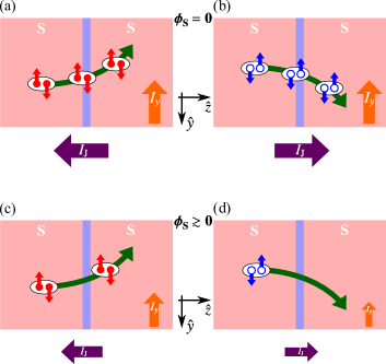
Figure 4: (a) Illustration of the electron Cooper pair tunneling from the left into the right S across the F-I barrier (light blue), generating the (tunneling) Josephson current, $I_{\mathrm{J}}$, and, owing to the skew tunneling mechanism (illustrated by the green arrows), the transverse AJHE current, $I_{y}$; the superconducting phase difference is $\phi_{\mathrm{S}}=0$ and the current amplitudes are proportional to the size of the violet and orange arrows. (b) Same as in (a), but for the tunneling of hole Cooper pairs from the left into the right S, essentially modeling electron Cooper pair tunneling from right to left. At $\phi_{\mathrm{S}}=0$, $I_{\mathrm{J}}$’s amplitude is the same as in (a), but the current flows along the opposite direction (recall that hole currents enter with opposite signs). The overall (tunneling) Josephson current vanishes. The transverse AJHE currents (both have again the same magnitude), contrarily, flow along the same direction and become maximal. (c), (d) Same as in (a) and (b), but at $\phi_{\mathrm{S}}\gtrsim 0$. Finite phase introduces a “bias” so that more electron Cooper pairs tunnel from left to right than vice versa and the overall (tunneling) Josephson current slowly starts to increase (the contributions no longer completely compensate, though they are both smaller than at $\phi_{\mathrm{S}}=0$). The decrease of the (tunneling) Cooper pair currents simultaneously damps their contributions to the generated AJHE current.

All supercurrent flows through the junction are essentially generated by the tunneling of Cooper pairs from one into the other S, each happening with certain probabilities. At zero superconducting phase difference ($\phi_{\mathrm{S}}=0$), tunnelings of Cooper pairs from the left into the right S and vice versa become equally likely. All Cooper pairs leaving one S are therefore fully compensated by others entering this S and no net (tunneling) Josephson currents flow; see Figs. 4(a)–(b) for illustration (the tunneling of Cooper pairs from right to left is modeled in terms of hole Cooper pairs that tunnel from left to right). Increasing $\phi_{\mathrm{S}}$ acts now as an effective “bias”. While the probability for forward tunneling (meaning from the left into the right S) is only barely affected, backward tunneling (meaning from the right into the left S) becomes much less likely. In the end, more (electron) Cooper pairs are transferred into the right S than leave, giving rise to a finite (tunneling) Josephson current. The imbalance (“bias”) between forward and backward tunnelings gets more distinct with further enhancing $\phi_{\mathrm{S}}$ so that simultaneously the (tunneling) Josephson current rises. Owing to the tunneling probabilities’ periodicity, the situation eventually reverses at $\phi_{\mathrm{S}}\approx\pi/2$ (assuming ideal or dirty junctions; otherwise the reversal happens at other values of $\phi_{\mathrm{S}}$) and the Josephson current decreases again, finally resembling the typical sinusoidal Josephson current-phase relation.

In sharp contrast, the AJHE current contributions stemming from forward and backward tunneling of Cooper pairs flow along the same direction and thus add up. As a consequence, the largest AJHE currents appear whenever forward and backward tunnelings become maximal (and equal in magnitudes), i.e., precisely at $\phi_{\mathrm{S}}=0\,\,(\mathrm{mod}\,\pi)$, as calculated in Fig. 3. Increasing $\phi_{\mathrm{S}}$ then primarily suppresses backward tunneling and simultaneously the total AJHE currents; see Figs. 4(c) and 4(d) for illustration.

V Bound state picture—SOC asymmetries

The formation of interfacial subgap bound states counts to the most distinct spectroscopic characteristics of Josephson junctions. Particularly interesting is the case in which the junctions additionally comprise magnetic components and the bound state spectrum splits into ABS and YSR branches. The latter turned out to possess unique spectral properties Vecino et al. (2003); Kawabata et al. (2012); Costa et al. (2018); Rouco et al. (2019) already in one-dimensional point contacts.

Those states are especially relevant to our study since all electrical current inside the F-I barrier is essentially carried by single electrons, which initially formed Cooper pairs in one of the superconductors, and now tunnel through the barrier via the available bound states. Each bound state occupied by an electron characteristically contributes to the (tunneling) Josephson and the AJHE currents. Instead of dealing with the Furusaki–Tsukada approach (see Sec. IV), one can equivalently access the current components via the bound state wave functions. The full calculations are rather cumbersome and can be looked up in Appendix B and the SM Note (2). The resulting interfacial AJHE currents, $I_{\eta}$, read as

$$I_{\eta} =-e\sum_{E_{\mathrm{B}}}\frac{|\Delta_{\mathrm{S}}(0)|\tanh\left(1.74\sqrt{T_{\mathrm{C}}/T-1}\right)}{2E_{\mathrm{B}}}$$

$$\hskip 10.0pt\times\frac{A}{(2\pi)^{2}}\int\mathrm{d}^{2}\mathbf{k}_{\parallel}\,\frac{\hbar k_{\eta}}{m}\left[\big{|}e(\mathbf{k}_{\parallel};E_{\mathrm{B}})\big{|}^{2}+\big{|}f(\mathbf{k}_{\parallel};E_{\mathrm{B}})\big{|}^{2}\right.$$

$$\hskip 20.0pt\left.+\big{|}g(\mathbf{k}_{\parallel};E_{\mathrm{B}})\big{|}^{2}+\big{|}h(\mathbf{k}_{\parallel};E_{\mathrm{B}})\big{|}^{2}\right]\times\tanh\left(\frac{E_{\mathrm{B}}}{2k_{\mathrm{B}}T}\right),$$ (5)

where $E_{\mathrm{B}}$ refers to the bound states’ energies (ABS and YSR states), while $e(\mathbf{k}_{\parallel};E_{\mathrm{B}})$, $f(\mathbf{k}_{\parallel};E_{\mathrm{B}})$, $g(\mathbf{k}_{\parallel};E_{\mathrm{B}})$, and $h(\mathbf{k}_{\parallel};E_{\mathrm{B}})$ represent the electronlike and holelike coefficients of the underlying bound state wave function (see Appendix B and the SM Note (2) for details). The thermal occupation factor, $\tanh[E_{\mathrm{B}}/(2k_{\mathrm{B}}T)]$, ensures that only occupied states are counted to the current. Simply speaking, the AJHE currents are given by the electrons’ transverse velocities, $v_{\eta}=(\hbar k_{\eta})/m$, multiplied by their charge, $-e$, and a “weighting factor”, which is mostly determined by the bound state energy (via the wave function coefficients).

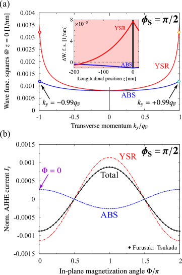
Figure 5: (a) Calculated absolute squares of the bound state wave functions at the F-I interface ($z=0$) as a function of the transverse momentum $k_{y}$ (normalized to the Fermi wave vector, $q_{\mathrm{F}}$) and for the superconducting phase difference $\phi_{\mathrm{S}}=\pi/2$; for simplicity, we set $k_{x}=0$ and $\Phi=0$. The Rashba SOC strength is $\overline{\lambda}_{\mathrm{R}}=(2m\alpha)/\hbar^{2}=1$ and all other parameters are the same as in Fig. 3. The blue curve corresponds to ABS and the red curve to YSR states. The inset shows the spatial dependence of the bound state wave functions’ absolute square differences, exemplarily in the left S and for $k_{y}=\pm 0.99q_{\mathrm{F}}$, as a deeper analysis Note (2) suggests that the dominant current contributions stem from states with $|\mathbf{k}_{\parallel}|\to q_{\mathrm{F}}$. The positive YSR tail indicates that the wave function squares at $k_{y}=0.99q_{\mathrm{F}}$ exceed those at $k_{y}=-0.99q_{\mathrm{F}}$ (and vice versa for the ABS). Though being small (as expected from the small AJHE currents), the $k_{y}$-asymmetry explained in the text becomes clearly evident. (b) Dependence of $I_{y}$ on $\Phi$ [same normalization as in Fig. 3 and for $\overline{\lambda}_{\mathrm{R}}=(2m\alpha)/\hbar^{2}=1$], calculated from the bound state spectrum. The contributions of ABS and YSR states are separately resolved; all other parameters are the same as in Fig. 3, except $\phi_{\mathrm{S}}=\pi/2$. As a cross-check, the dots show the total AJHE current evaluated from the Furusaki–Tsukada approach.

As long as the interfacial SOC remains absent, the junction’s bound state spectrum is symmetric with respect to a reversal of $\mathbf{k}_{\parallel}$. To each electron with transverse velocity $v_{\eta}=(\hbar k_{\eta})/m$, being transferred through the F-I via a bound state at energy $E_{\mathrm{B}}$, one finds a second electron with opposite velocity ($-v_{\eta}$), occupying a bound state with precisely the same energy. Consequently, two occupied states always carry the same amount of current along opposite directions so that the overall AJHE currents vanish. Since SOC scales linearly with the components of $\mathbf{k}_{\parallel}=[k_{x},\,k_{y},\,0]^{\top}$, nonzero SOC causes an asymmetry of the bound state energies with respect to $\mathbf{k}_{\parallel}$’s sign. Depending on the chosen SOC strength and the magnetic tunneling parameter, the energies of the bound states getting occupied by the propagating (with transverse velocity $v_{\eta}$) and its counterpropagating (with transverse velocity $-v_{\eta}$) electron are no longer identical and may noticeably differ. In contrast to the case without SOC, the current contributions stemming from the propagating and counterpropagating states cannot fully compensate [as the energy-dependent “weighting factors” entering Eq. (5) differ once the $E_{\mathrm{B}}$’s of the propagating and counterpropagating states are no longer equal], and finite AJHE currents start to flow. Such SOC-controlled $\mathbf{k}_{\parallel}$-asymmetries in the bound state energies are thus the microscopic physical manifestation of the AJHE.

Figure 5(a) illustrates this asymmetry for $k_{y}$ (keeping $k_{x}=0$ fixed) and the same parameters as considered in Fig. 3, except that we additionally assume $\phi_{\mathrm{S}}=\pi/2$ to stress that our explanations are general and not restricted to zero phase difference. Since the SOC asymmetry of the bound state energies is rather small and hard to visualize (owing to the small $\lambda_{\mathrm{MA}}$ used for our calculations), we focus on the absolute squares of the bound state wave functions (see the SM Note (2) for details). Apparently, the $k_{y}$-asymmetry is more pronounced for the YSR than for the ABS branch of the spectrum. Furthermore, the SOC asymmetry impacts the ABS and the YSR states in the opposite way. While the YSR states’ wave function squares are raised at $k_{y}>0$, those belonging to ABS decrease there. Translating both observations into current flows, we expect that the single current contributions stemming from the two bound state bands must flow along opposite directions and the YSR part must be the dominant one. This is also the deeper reason why sizable AJHE currents require not only interfacial SOC, but also (at least weak) ferromagnetism. If the latter would not be there, the bound state bands simply merge into the usual ABS and the $\mathbf{k}_{\parallel}$-asymmetry (and simultaneously the AJHE) immediately disappear.

Evaluating the AJHE currents from Eq. (5) [see Fig. 5(b)] essentially confirms all predicted features. The AJHE currents obtained from the bound state spectrum coincide with the results extracted from the Furusaki–Tsukada approach. Although the first method is computationally more challenging and less general, it establishes an important cross-check for the second technique and brings along more physical insight. For example, the spatial dependence of the bound state wave function squares [see Fig. 5(a)] allows us to deduce the AJHE currents’ spatial dependence, which was not covered by the Furusaki–Tsukada formula (we computed the currents at the interface there). Since the squares of the wave function coefficients directly enter the bound state current formula [see Eq. (5)], the AJHE currents decay in exactly the same way with increasing distance from the interface, i.e., exponentially over the characteristic decay length $\kappa=1/\{2\mathrm{Im}[q_{z,\mathrm{e}}(E_{\mathrm{B}})]\}$, where $q_{z,\mathrm{e}}(E_{\mathrm{B}})=q_{\mathrm{F}}[1+\mathrm{i}(|\Delta_{\mathrm{S}}|^{2}-E_{\mathrm{B}}^{2})^{1/2}/\mu-\mathbf{k}_{\parallel}^{2}/q_{\mathrm{F}}^{2}]^{1/2}$ indicates the electronlike wave vector inside the superconductors. We provide a more comprehensive discussion of the SOC-induced $\mathbf{k}_{\parallel}$-asymmetries, with special attention on the bound state spectra and their correlation to the AJHE currents, in the SM Note (2).

VI Transverse spin currents

Apart from the AJHE charge currents, also their spin current counterparts might provide indispensable ingredients for spintronics applications. When tunneling through the spin-active F-I barrier, some of the spin-singlet Cooper pairs’ electrons undergo spin flips and generate spin-polarized triplet pairs Ouassou et al. (2017). Those pairs’ spin wave functions may be composed of all possible triplet pairings, $|{\uparrow\uparrow}\rangle$, $|{\downarrow\downarrow}\rangle$, and $(|{\uparrow\downarrow}\rangle+|{\downarrow\uparrow}\rangle)/\sqrt{2}$, where $|{\uparrow}\rangle$ ($|{\downarrow}\rangle$) denotes a single electron up-spin (down-spin) state with respect to the $\hat{z}$-spin quantization axis (inside the superconductors). The $(|{\uparrow\downarrow}\rangle+|{\downarrow\uparrow}\rangle)/\sqrt{2}$-contribution is usually neglected since it decays rapidly inside real tunneling barriers Ouassou et al. (2017). The remaining $|{\uparrow\uparrow}\rangle$- and $|{\downarrow\downarrow}\rangle$-pairs, however, are also subject to the proposed skew tunneling mechanism and may separate along the transverse directions. From that point of view, skew tunneling acts like a transverse Cooper pair spin filter and generates nonzero transverse spin supercurrent flows, combining the advantages of the conventional spin Hall effect (referring to pure transverse spin currents in the absence of charge currents) Dyakonov and Perel (1971a, b); *Dyakonov1971a with the dissipationless character of supercurrents.

Anyhow, earlier studies Mal’shukov and Chu (2008) demonstrated that superconductors’ fundamental time-reversal (electron–hole) symmetry suppresses the spin Hall effect. The recent prediction of sizable tunneling spin Hall currents in metal/insulator/metal junctions Matos-Abiague and Fabian (2015), essentially triggered by interfacial skew tunneling just as in our study, boosted new hopes to efficiently integrate the spin Hall effect into superconducting tunnel junction geometries. Nonetheless, replacing one of the junction’s normal-conducting electrodes by a S will dramatically impact the underlying physics. The resulting strong competition between skew ARs and skew SRs (being another consequence of the electron–hole symmetry) will again heavily suppress the tunneling spin Hall currents Note (2).

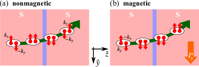
Figure 6: (a) Illustration of the Cooper pair skew tunneling from the left into the right S across the F-I barrier (light blue). Each Cooper pair initially consists of one up-spin electron with transverse momentum $k_{y}>0$ and one down-spin electron with $-k_{y}$ (assuming, for simplicity, $k_{x}=0$). When tunneling through the spin-active interface, at which the present SOC gives rise to nonzero spin-flip probabilities, some Cooper pair electrons flip their spins, converting spin-unpolarized singlet into spin-polarized triplet pairs. In the absence of exchange coupling ($\lambda_{\mathrm{MA}}=0$), interfacial spin flips generate, on average, the same amount of polarized $|{\uparrow\uparrow}\rangle$- and $|{\downarrow\downarrow}\rangle$-Cooper pairs (per transverse channel) so that eventually the overall transverse spin current vanishes. (b) If exchange coupling is present ($\lambda_{\mathrm{MA}}\neq 0$), interfacial spin flips cause an excess of either $|{\uparrow\uparrow}\rangle$- or $|{\downarrow\downarrow}\rangle$-pairs in the skew tunneling channel along $-\hat{y}$ (and vice versa along $\hat{y}$). The result is a finite transverse spin supercurrent, denoted by $I_{y}^{\mathrm{s}}$ and highlighted by the orange arrow.

Before we evaluate the transverse spin current components that flow through our Josephson junction, we therefore need to understand the connections between the triplet pair skew tunneling and the generated transverse spin currents. Both superconductors act as reservoirs for spin-singlet Cooper pairs, each consisting of two electrons with opposite spin and antiparallel momenta (recall that $\mathbf{k}_{\parallel}=[k_{x},\,k_{y},\,0]^{\top}$). To be more specific, the allowed spin and transverse momenta configurations of the Cooper pairs are $({\mathbf{k}_{\parallel},\uparrow};{-\mathbf{k}_{\parallel},\downarrow})$, $({-\mathbf{k}_{\parallel},\downarrow};{\mathbf{k}_{\parallel},\uparrow})$, $({\mathbf{k}_{\parallel},\downarrow};{-\mathbf{k}_{\parallel},\uparrow})$, and $({-\mathbf{k}_{\parallel},\uparrow};{\mathbf{k}_{\parallel},\downarrow})$; the two parts always indicate the transverse momentum and spin of the two electrons forming a singlet pair. Approaching the barrier, the Cooper pairs are exposed to the aforementioned skew tunneling mechanism. As a consequence, they are spatially separated along the transverse $\hat{\eta}\in\{\hat{x};\hat{y}\}$-directions, i.e., if the $({\mathbf{k}_{\parallel},\uparrow};{-\mathbf{k}_{\parallel},\downarrow})$- and $({-\mathbf{k}_{\parallel},\downarrow};{\mathbf{k}_{\parallel},\uparrow})$-pairs are predominantly transmitted at $\eta<0$, the remaining pairs tunnel mostly at positive $\eta$. For a further characterization, we distinguish between nonmagnetic and magnetic junctions.

Nonmagnetic junctions.

As long as the barrier is nonmagnetic, the numbers of Cooper pairs involved in the skew tunneling processes at $\eta<0$ and $\eta>0$ are always equal. Therefore, both channels generate the same charge current flows along reversed directions and no net transverse charge currents build up. Close to the barrier, the interfacial SOC gives additionally rise to nonzero spin-flip probabilities, determined by the respective spin-flip potential, $V_{\mathrm{flip}}$. In the nonmagnetic junction (and assuming $\beta=0$, as well as $k_{x}=0$, to further simplify our considerations), we deduce $V_{\mathrm{flip}}\sim\alpha k_{y}\sigma$, where $k_{y}$ and $\sigma$ denote one Cooper pair electron’s $\hat{y}$-component of $\mathbf{k}_{\parallel}$ and its spin [note the close analogy with Eq. (3)]. In our case, this means that an up-spin electron with $k_{y}>0$ flips its spin with the same probability as a down-spin electron with $-k_{y}$. On average, each transverse skew tunneling channel (along $\pm\hat{y}$) contains then the same amount of $|{\uparrow\uparrow}\rangle$- and $|{\downarrow\downarrow}\rangle$-triplet pairs, and the overall transverse spin current components must vanish [see Fig. 6(a) for illustration]. To get the full picture, one would also need to include the electron Cooper pairs tunneling from right to left (or hole pairs tunneling from left to right). Since similar arguments apply to hole Cooper pairs, this would still not lead to finite transverse spin currents.

Magnetic junctions.

The situation starts to change if the barrier becomes (at least weakly) magnetic. The Cooper pair electrons’ spin-flip probabilities are then governed by the spin-flip potential $V_{\mathrm{flip}}\sim(\lambda_{\mathrm{MA}}\sin\Phi)\sigma+\alpha k_{y}\sigma$, and become asymmetric with respect to the electrons’ spins. A $k_{y}$-electron with spin up flips its spin now with a different probability than a $(-k_{y})$-spin down electron. Therefore, the skew tunneling channel along $-\hat{y}$ comprises an excess of either $|{\uparrow\uparrow}\rangle$- or $|{\downarrow\downarrow}\rangle$-pairs and the channel along $\hat{y}$ either more $|{\downarrow\downarrow}\rangle$- or $|{\uparrow\uparrow}\rangle$-pairs. The result is a nonzero transverse spin current; see Fig. 6(b). Note that, aside from the configuration involving magnetic barriers, one could achieve similar effects, e.g., by replacing one of the superconducting electrodes by a two-dimensional S with strong bulk Rashba SOC Zhi-Hong et al. (2012). Furthermore, our qualitative explanations suggest that a reversal of $\lambda_{\mathrm{MA}}$’s sign must be sufficient to reverse the direction of the spin current (since this simultaneously reverses the sign of the spin-dependent magnetization part of $V_{\mathrm{flip}}$).

To access and quantify the particle  spin currents in our junction, we can either generalize the Furusaki–Tsukada technique or our bound state approach. Within an extended Furusaki–Tsukada formulation Asano (2005), the interfacial $\hat{\sigma}_{z}$-spin currents along the $\hat{\eta}$-direction are given by

$$\small I_{\eta,\hat{z}}^{\mathrm{s}}\approx\frac{k_{\mathrm{B}}T}{4}|\Delta_{\mathrm{S}}(0)|\tanh\left(1.74\sqrt{\frac{T_{\mathrm{C}}}{T}-1}\right)\frac{A}{(2\pi)^{2}}\int\mathrm{d}^{2}\mathbf{k}_{\parallel}\,\sum_{\omega_{n}}\frac{k_{\eta}}{\sqrt{q_{\mathrm{F}}^{2}-\mathbf{k}_{\parallel}^{2}}}\left[\frac{\mathcal{C}^{(1)}(\mathrm{i}\omega_{n})-\mathcal{D}^{(2)}(\mathrm{i}\omega_{n})-\mathcal{A}^{(3)}(\mathrm{i}\omega_{n})+\mathcal{B}^{(4)}(\mathrm{i}\omega_{n})}{\sqrt{\omega_{n}^{2}+|\Delta_{\mathrm{S}}(0)|^{2}\tanh^{2}\left(1.74\sqrt{T_{\mathrm{C}}/T-1}\right)}}\right],$$ (6)

while the bound state modeling yields

$$I_{\eta,\hat{z}}^{\mathrm{s}}=\frac{\hbar}{2}\sum_{E_{\mathrm{B}}}\frac{|\Delta_{\mathrm{S}}(0)|\tanh\left(1.74\sqrt{T_{\mathrm{C}}/T-1}\right)}{2E_{\mathrm{B}}}\frac{A}{(2\pi)^{2}}\int\mathrm{d}^{2}\mathbf{k}_{\parallel}\,\frac{\hbar k_{\eta}}{m}\left[\big{|}e(\mathbf{k}_{\parallel};E_{\mathrm{B}})\big{|}^{2}-\big{|}f(\mathbf{k}_{\parallel};E_{\mathrm{B}})\big{|}^{2}-\big{|}g(\mathbf{k}_{\parallel};E_{\mathrm{B}})\big{|}^{2}+\big{|}h(\mathbf{k}_{\parallel};E_{\mathrm{B}})\big{|}^{2}\right]\tanh\left(\frac{E_{\mathrm{B}}}{2k_{\mathrm{B}}T}\right).$$ (7)

Reasoning for the two formulas is given in Appendix C and the SM Note (2).

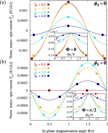
Figure 7: (a) Calculated dependence of the $\hat{\sigma}_{z}$-spin current along $\hat{x}$, $I_{x,\hat{z}}^{\mathrm{s}}$, given in units of $\hbar/(2e)$ and normalized according to $(I_{x,\hat{z}}^{\mathrm{s}}e)/[G_{\mathrm{S}}\pi|\Delta_{\mathrm{S}}(0)|]$, on the F-I’s in-plane magnetization angle, $\Phi$, and for the same parameters as considered in Fig. 3. The inset shows the maximal $I_{x,\hat{z}}^{\mathrm{s}}$ (i.e., for $\Phi=0$) as a function of the superconducting phase difference, $\phi_{\mathrm{S}}$. (b) Similar calculations as in (a) for the $\hat{\sigma}_{z}$-spin current along $\hat{y}$, $I_{y,\hat{z}}^{\mathrm{s}}$.

Figure 7 presents the numerically computed [by means of Eq. (6)] transverse spin current components, $I_{x,\hat{z}}^{\mathrm{s}}$ and $I_{y,\hat{z}}^{\mathrm{s}}$, for the same set of junction parameters considered when evaluating the AJHE charge currents in Fig. 3. As stated above, putting the F-I’s magnetic tunneling parameter to zero (which basically means that the barrier becomes nonmagnetic) would immediately lead to vanishing transverse spin currents. In contrast, already the weak magnetic tunneling strength assumed for our AJHE charge current calculations is sufficient to trigger sizable transverse spin current responses.

Regarding the spin currents’ dependence on the F-I’s in-plane magnetization angle, $\Phi$, we observe an experimentally promising trend. While the charge currents scale according to $I_{x}\sim\sin\Phi$ and $I_{y}\sim\cos\Phi$, the spin currents obey $I_{x,\hat{z}}^{\mathrm{s}}\sim\cos\Phi$ and $I_{y,\hat{z}}^{\mathrm{s}}\sim\sin\Phi$. These well-distinct $\Phi$-variations come along with another particularly auspicious property. The spin current components become maximal precisely at those magnetization angles at which the AJHE charge current counterparts simultaneously vanish. As a result, tuning the magnetization angle allows for an experimental switch between the pure AJHE charge current and the pure transverse spin current regimes. Owing to its analogy with conventional spin Hall effects, the latter phenomenon could be termed anomalous Josephson spin Hall effect; anomalous stresses that our junction needs to be weakly magnetic, in contrast to the conventional spin Hall effect which occurs already in nonmagnetic systems. Altering $\Phi$ essentially modulates the spin-flip potential, controlling the spin-flip probabilities of Cooper pair electrons and thereby the generation rate of triplet pairs. Particularly at $\Phi=\pi/2$, the negative amplitudes of $I_{y,\hat{z}}^{\mathrm{s}}$ indicate that each transverse skew tunneling channel along $\hat{y}$ involves an excess of $|{\downarrow\downarrow}\rangle$-pairs. Moreover, the spin-flip potential does not depend on the superconducting phase difference, $\phi_{\mathrm{S}}$. Thus, varying $\phi_{\mathrm{S}}$ does not qualitatively impact the spin current flow (i.e., not reverse its direction, in sharp contrast to the AJHE charge currents), but simply changes its overall amplitudes by introducing the “bias” between the mutually enhancing electron and hole Cooper pairs we encountered when analyzing the AJHE currents. At $\phi_{\mathrm{S}}=\pi$, maximal AJHE charge currents come again along with vanishing transverse spin currents, which might offer another interesting parameter configuration for following experiments. As claimed earlier when investigating the generic form of the spin-flip potential, switching the magnetic tunneling parameter’s sign would reverse the directions of the transverse spin currents.

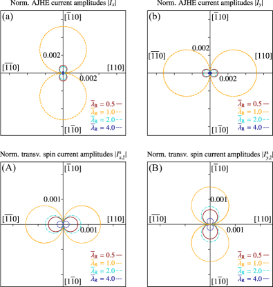
Figure 8: (a) Calculated angular dependence of the AJHE charge current amplitudes along $\hat{x}$, $I_{x}$, on the F-I’s in-plane magnetization angle, $\Phi$. All parameters and the normalization are the same as in Fig. 3, except that we assume $\overline{\lambda}_{\mathrm{D}}=(2m\beta)/\hbar^{2}=0$ now. (b) Similar calculations as in (a) for the AJHE charge current amplitudes along $\hat{y}$, $I_{y}$. (A), (B) Similar calculations as in (a) and (b), but for the transverse $\hat{\sigma}_{z}$-spin current amplitudes, $I_{x,\hat{z}}^{\mathrm{s}}$ and $I_{y,\hat{z}}^{\mathrm{s}}$, given in units of $\hbar/(2e)$ and normalized as in Fig. 7.

We also computed all AJHE charge and transverse spin current parts assuming that just Rashba SOC is present and Dresselhaus SOC is absent ($\beta\sim\overline{\lambda}_{\mathrm{D}}=0$); all remaining parameters were not changed. This situation might often be the experimentally more realistic one since tunneling barriers inevitably introduce interfacial Rashba SOC due to the broken space inversion symmetry, whereas only those additionally lacking bulk inversion symmetry give rise to nonzero Dresselhaus SOC. The results of our calculations are summarized in Fig. 8. Contrary to the tunneling Josephson (charge) current, whose magnetoanisotropy disappears if only either interfacial Rashba or Dresselhaus SOC is considered, the AJHE charge and spin currents’ still clearly reveal their unique and well-distinct scaling with respect to the magnetization angle we mentioned in the previous paragraph. Since $I_{x}\sim-(\alpha+\beta)\sin\Phi$ and $I_{y}\sim(\alpha-\beta)\cos\Phi$ (and adapted relations hold for the spin currents), the maximal amplitudes of the $\hat{x}$- and $\hat{y}$-current components become exactly equal once Dresselhaus SOC is no longer there (i.e., when setting $\beta=0$). For appropriately chosen Rashba SOC strengths, the current amplitudes can now even overcome those we extracted in the simultaneous presence of Rashba and Dresselhaus SOC. Measuring the currents’ angular dependencies for concrete junction geometries and fitting the results to our modeling might provide valuable insight into the characteristics of the system’s interfacial SOC.

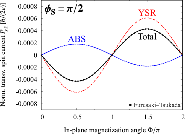
Figure 9: Calculated (from the bound state spectrum) dependence of the $\hat{\sigma}_{z}$-spin current along $\hat{y}$, $I_{y,\hat{z}}^{\mathrm{s}}$, given in units of $\hbar/(2e)$ and normalized as in Fig. 7, on the F-I’s in-plane magnetization angle, $\Phi$, for the Rashba SOC parameter $\overline{\lambda}_{\mathrm{R}}=(2m\alpha)/\hbar^{2}=1$ and the superconducting phase difference $\phi_{\mathrm{S}}=\pi/2$; all other parameters are the same as in Fig. 3. The individual contributions of ABS and YSR states are separately resolved. As a cross-check, the dots represent the total spin current extracted from the Furusaki–Tsukada formula.

Similarly to our analyses of the AJHE charge currents, we finally evaluate the transverse spin currents from the junction’s bound state spectrum [by means of Eq. (7)]. Figure 9 illustrates the total spin current along $\hat{y}$, $I_{y,\hat{z}}^{\mathrm{s}}$, together with its individual contributions stemming from the junction’s ABS and YSR states, and, for comparison, the related $I_{y,\hat{z}}^{\mathrm{s}}$ obtained from the Furusaki–Tsukada method [using Eq. (6)]. We regarded the same junction parameters as in Fig. 7 (i.e., Rashba and Dresselhaus SOC are both nonzero), except that we keep the superconducting phase difference at $\phi_{\mathrm{S}}=\pi/2$ (as in Fig. 5 to stress that the trends are general). Analogously to the AJHE charge currents, the transverse spin currents are also mostly dominated by the YSR states, which contribute again with an opposite sign to the overall spin current compared to the ABS. The negative (positive) sign of the YSR states (ABS) parts (at $0<\Phi<\pi$) actually entails that down-spin (up-spin) electrons with transverse momenta $\mathbf{k}_{\parallel}=[k_{x}>0,\,k_{y}>0,\,0]^{\top}$ tunnel predominantly through the F-I interface via the available YSR states (ABS). This observation has its physical origin in the peculiar spin characteristics associated with ABS and YSR states in magnetic Josephson junctions Costa et al. (2018). For the considered parameters, the YSR states (at fixed $\mathbf{k}_{\parallel}=[k_{x}>0,\,k_{y}>0,\,0]^{\top}$) correspond to down-spin states (through which the down-spin Cooper pair electrons tunnel) and the ABS to up-spin states (through which the up-spin Cooper pair electrons tunnel); see the comprehensive analysis of the states’ spin characteristics provided in Ref. Costa et al. (2018). An excess of down-spin electrons with momentum $\mathbf{k}_{\parallel}$ that skew tunnel through the interface yields a negative spin current (essentially, this is then precisely the case for the YSR states) and an excess of up-spin electrons (in the ABS) a positively counted spin current contribution. The perfect agreement of the bound state and the Furusaki–Tsukada approach persuades that our results are reliable.

Spin–charge current cross ratios.

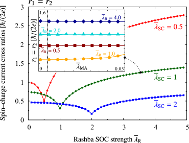
Figure 10: Calculated dependence of the universal spin–charge current cross ratios, $r_{1}$ and $r_{2}$, given in units of $\hbar/(2e)$, on the Rashba SOC strength, $\overline{\lambda}_{\mathrm{R}}=(2m\alpha)/\hbar^{2}$. Since the Dresselhaus SOC parameter is $\overline{\lambda}_{\mathrm{D}}=(2m\beta)/\hbar^{2}=0$, $r_{1}=r_{2}$; all other parameters are the same as in Fig. 3 (i.e., also $\phi_{\mathrm{S}}=0$), except that the scalar tunneling gets gradually increased from $\overline{\lambda}_{\mathrm{SC}}=(2m\lambda_{\mathrm{SC}})/(\hbar^{2}q_{\mathrm{F}})=0.5$ (red) to $\overline{\lambda}_{\mathrm{SC}}=1$ (dark green), and finally to $\overline{\lambda}_{\mathrm{SC}}=2$ (blue). The inset shows $r_{1}$ ($=r_{2}$) as a function of the magnetic tunneling parameter, $\overline{\lambda}_{\mathrm{MA}}=(2m\lambda_{\mathrm{MA}})/(\hbar^{2}q_{\mathrm{F}})$, and for various Rashba SOC parameters, $\overline{\lambda}_{\mathrm{R}}=(2m\alpha)/\hbar^{2}$ (again assuming $\overline{\lambda}_{\mathrm{D}}=(2m\beta)/\hbar^{2}=0$ for the Dresselhaus SOC); $\overline{\lambda}_{\mathrm{SC}}=(2m\lambda_{\mathrm{SC}})/(\hbar^{2}q_{\mathrm{F}})=1$ is kept constant. The dotted vertical line indicates $\overline{\lambda}_{\mathrm{MA}}=0.005$, which we assumed for all previous calculations and for which the $r$-ratios become indeed universal.

In weakly magnetic junctions, both the AJHE charge and transverse spin currents increase linearly with the magnetic tunneling parameter, $\overline{\lambda}_{\mathrm{MA}}$. The spin–charge current cross ratios ,

$$r_{1}:=\left|\frac{I_{x,\hat{z}}^{\mathrm{s}}}{I_{y}}\right|\quad\quad\text{and}\quad\quad r_{2}:=\left|\frac{I_{y,\hat{z}}^{\mathrm{s}}}{I_{x}}\right|,$$ (8)

turn then into universal, magnetization-independent, measures, which are uniquely determined by the interfacial SOC strengths (keeping $\overline{\lambda}_{\mathrm{SC}}$ and $\phi_{\mathrm{S}}$ constant, and restricting ourselves to parameters for which all currents are nonzero). If only Rashba SOC is present, both ratios become equal ($r_{1}=r_{2}$), whereas the constructive (destructive) interferences of finite Rashba and Dresselhaus SOC impact the $\hat{x}$- and $\hat{y}$-currents in a different manner so that generally $r_{1}\neq r_{2}$ (as $r_{1}$ and $r_{2}$ basically relate $\hat{x}$- and $\hat{y}$-currents at the same time). Figure 10 illustrates the spin–charge current cross ratios’ characteristic scaling with respect to the Rashba SOC parameter, $\overline{\lambda}_{\mathrm{R}}$, in the absence of Dresselhaus SOC ($\overline{\lambda}_{\mathrm{D}}=0$). Extracting $r_{1}$ and $r_{2}$ from experimental transport data and fitting the results to our model provides one way to identify the SOC parameters of the junction’s F-I interface, without having exact knowledge of $\overline{\lambda}_{\mathrm{MA}}$ or the magnetization orientation.

As soon as $\overline{\lambda}_{\mathrm{MA}}$ overcomes some critical value, the charge and spin current parts are additionally governed by nonlinear $\overline{\lambda}_{\mathrm{MA}}$-terms and the $r$-ratios are no longer universal quantities of the system. To estimate the relevance of these nonlinearities, the inset of Fig. 10 shows $r_{1}$ ($r_{1}=r_{2}$ since Dresselhaus SOC is not present) as a function of $\overline{\lambda}_{\mathrm{MA}}$ and for various Rashba SOC strengths. Apparently, the spin–charge current cross ratios remain indeed universal (magnetization independent) for the small magnetic tunneling strengths considered in all previously discussed current calculations (i.e., for $\overline{\lambda}_{\mathrm{MA}}\approx 10^{-3}$) and can therefore be used to reliably quantify the present SOC in experiments. Nonlinear $\overline{\lambda}_{\mathrm{MA}}$-terms do not affect the AJHE charge and spin currents unless $\overline{\lambda}_{\mathrm{MA}}$ gets further enhanced by at least one order of magnitude.

Another peculiar feature becomes visible once the Rashba SOC measure approaches the scalar tunneling strength, i.e., at $\overline{\lambda}_{\mathrm{R}}\approx\overline{\lambda}_{\mathrm{SC}}$, as the spin–charge current cross ratios’ amplitudes always drop into a sharp dip there. To strengthen the generality of this observation, we considered three different $\overline{\lambda}_{\mathrm{SC}}$-values in Fig. 10, essentially all causing the same behavior. Recalling our qualitative picture formulated in Sec. III, the AJHE charge currents are generated by skew ARs of incident up-spin and down-spin electrons at the effective interfacial scattering potential. The latter is stated in Eq. (3) for the limiting case of restricting ourselves to the current along $\hat{y}$, $I_{y}$; similar arguments hold, nevertheless, also for the $I_{x}$-current. Inspecting Eq. (3), we deduce that incoming down-spin (up-spin) electrons are exposed to the lowest (largest) possible interfacial scattering potential exactly when the Rashba SOC and the scalar tunneling measures become equal. As a result, the down-spin channel carries its maximal amount of AJHE current, while the (oppositely oriented) contribution of the up-spin channel becomes simultaneously minimal. The overall AJHE current, $I_{y}$, reaches its maximal value and even significantly overcomes the related spin currents. Our numerical calculations discussed in Figs. 8(a)–8(d) essentially confirm these characteristics. Note that Dresselhaus SOC is not present; otherwise, the interference of Rashba and Dresselhaus terms would give rise to more intricate features. Since the AJHE charge currents enter the spin–charge current cross ratios’ denominators, maximal $I_{y}$ ($I_{x}$) eventually comes along with strongly suppressed $r$-ratios, manifested by the $r$-$\overline{\lambda}_{\mathrm{R}}$ relations’ sharp dips at $\overline{\lambda}_{\mathrm{R}}\approx\overline{\lambda}_{\mathrm{SC}}$. Moreover, an increase of $\overline{\lambda}_{\mathrm{SC}}$ notably damps the current cross ratios at large Rashba SOC ($\overline{\lambda}_{\mathrm{R}}>\overline{\lambda}_{\mathrm{SC}}$) since strong interfacial scalar tunneling usually suppresses the generated spin currents much faster than their charge current counterparts.

VII Summary

To conclude, we investigated the intriguing interplay of SOC and ferromagnetism arising at the interface of S/F-I/S Josephson junctions. Starting from simplified qualitative arguments, we understood that skew tunneling of Cooper pairs through the spin-active interface can give rise to spontaneous transverse AJHE charge current flows, which may become relevant to various superconducting spintronics applications, especially due to their dissipationless character and their wide tunability. We demonstrated the latter by evaluating the AJHE current amplitudes from a generalized Furusaki–Tsukada Green’s function technique and for a variety of realistic junction parameters. The interfacial Rashba SOC strength, which is mostly determined by the material composition of the system, and the magnetically adjustable phase difference between the superconductors offer particularly auspicious possibilities to vary the AJHE current magnitudes over several orders of magnitude. Maximal AJHE currents can reach a few percent of the (tunneling) Josephson current and thereby significantly exceed normal-state TAHE conductances, which remain usually far below $1\,\%$ of the respective tunneling conductances Matos-Abiague and Fabian (2015). The AJHE currents’ unique sinelike (cosinelike) variations with the magnetization angle inside the F-I were identified as a clear evidence that all the fascinating physics really stems from the combination of SOC with ferromagnetism in one single junction.

To establish an alternative approach, which brings along more physical insight, we connected nonzero AJHE currents to pronounced SOC-induced asymmetries in the junctions’ ABS and YSR bound state energies, and elucidated that the AJHE on the one hand and these bound state energy asymmetries on the other hand are uniquely correlated. Resolving the individual states’ current contributions, we convinced ourselves that the huge AJHE current flows are predominantly maintained by the YSR states, whose appearance counts to the most peculiar features of magnetic Josephson junctions.

Finally, we outlined that SOC triggers interfacial spin flips of Cooper pair electrons and produces spin-polarized triplet pairs. Since these triplet pairs are also subject to the skew tunneling mechanism, while carrying a net spin, we proposed that the AJHE charge current phenomena come along with their transverse spin current counterparts. We qualitatively unraveled the spin currents’ general properties and computed their amplitudes once from Green’s functions and once exploiting the bound state asymmetries, again revealing a great tunability by means of the Rashba SOC parameter or the superconducting phase difference. We illustrated the spin currents’ well-distinct magnetization angle dependence when compared to the AJHE charge currents and characterized the universal (magnetization-independent) spin–charge current cross ratios, which might provide a valuable experimental tool to probe interfacial SOC in superconducting tunnel junctions.

Appendix A Generalized Furusaki–Tsukada method

Assuming translational invariance parallel to the F-I interface, the solutions of the BdG equation, $\hat{\mathcal{H}}_{\mathrm{BdG}}\Psi(\mathbf{r})=E\Psi(\mathbf{r})$, describing quasiparticle excitations of energy $E$, factorize into

$$\Psi(\mathbf{r})=\psi(z)\mathrm{e}^{\mathrm{i}(\mathbf{k}_{\parallel}\cdot\mathbf{r}_{\parallel})};$$ (9)

$\mathbf{k}_{\parallel}=[k_{x},\,k_{y},\,0]^{\top}$ ($\mathbf{r}_{\parallel}=[x,\,y,\,0]^{\top}$) refers to the transverse wave vector (vector of transverse spatial coordinates). Substituting Eq. (9) into the BdG equation, the most general solutions for the $\hat{z}$-projected scattering states inside the superconductors are found to read as

$$\psi^{(i)}(z<0)=\psi^{(i)}_{\mathrm{incoming}}(z<0)\\ +\mathcal{A}^{(i)}\left[\begin{matrix}u\\ \phantom{a}0\phantom{a}\\ v\\ 0\end{matrix}\right]\mathrm{e}^{-\mathrm{i}q_{z,\mathrm{e}}z}+\mathcal{B}^{(i)}\left[\begin{matrix}\phantom{a}0\phantom{a}\\ u\\ 0\\ v\end{matrix}\right]\mathrm{e}^{-\mathrm{i}q_{z,\mathrm{e}}z}\\ +\mathcal{C}^{(i)}\left[\begin{matrix}v\\ \phantom{a}0\phantom{a}\\ u\\ 0\end{matrix}\right]\mathrm{e}^{\mathrm{i}q_{z,\mathrm{h}}z}+\mathcal{D}^{(i)}\left[\begin{matrix}\phantom{a}0\phantom{a}\\ v\\ 0\\ u\end{matrix}\right]\mathrm{e}^{\mathrm{i}q_{z,\mathrm{h}}z},$$ (10)

as well as

$$\psi^{(i)}(z>0)=\mathcal{E}^{(i)}\left[\begin{matrix}u\mathrm{e}^{\mathrm{i}\phi_{\mathrm{S}}}\\ 0\\ v\\ 0\end{matrix}\right]\mathrm{e}^{\mathrm{i}q_{z,\mathrm{e}}z}+\mathcal{F}^{(i)}\left[\begin{matrix}0\\ u\mathrm{e}^{\mathrm{i}\phi_{\mathrm{S}}}\\ 0\\ v\end{matrix}\right]\mathrm{e}^{\mathrm{i}q_{z,\mathrm{e}}z}\\ +\mathcal{G}^{(i)}\left[\begin{matrix}v\mathrm{e}^{\mathrm{i}\phi_{\mathrm{S}}}\\ 0\\ u\\ 0\end{matrix}\right]\mathrm{e}^{-\mathrm{i}q_{z,\mathrm{h}}z}+\mathcal{H}^{(i)}\left[\begin{matrix}0\\ v\mathrm{e}^{\mathrm{i}\phi_{\mathrm{S}}}\\ 0\\ u\end{matrix}\right]\mathrm{e}^{-\mathrm{i}q_{z,\mathrm{h}}z},$$ (11)

where the electronlike and holelike wave vectors’ $\hat{z}$-projections are given by

$$q_{z,\mathrm{e}} =q_{z,\mathrm{e}}(\mathbf{k}_{\parallel};E)=\sqrt{\frac{2m}{\hbar^{2}}\left[\mu+\sqrt{E^{2}-|\Delta_{\mathrm{S}}|^{2}}\right]-\mathbf{k}_{\parallel}^{2}}$$ (12)

and

$$q_{z,\mathrm{h}} =q_{z,\mathrm{h}}(\mathbf{k}_{\parallel};E)=\sqrt{\frac{2m}{\hbar^{2}}\left[\mu-\sqrt{E^{2}-|\Delta_{\mathrm{S}}|^{2}}\right]-\mathbf{k}_{\parallel}^{2}},$$ (13)

and the coherence factors, $u=u(E)$ and $v=v(E)$, need to satisfy

$$u(E)=\sqrt{\frac{1}{2}\left(1+\sqrt{1-\frac{|\Delta_{\mathrm{S}}|^{2}}{E^{2}}}\right)}=\sqrt{1-v^{2}(E)}.$$ (14)

The incoming waves, $\psi_{\mathrm{incoming}}^{(i)}$, differentiate between (1) up-spin electronlike, (2) down-spin electronlike, (3) up-spin holelike, and (4) down-spin holelike quasiparticles incident on the F-I from the left superconductor. Formally, they can be written as

$$\psi^{(1)}_{\mathrm{incoming}}(z<0) =[u,\,0,\,v,\,0]^{\top}\mathrm{e}^{\mathrm{i}q_{z,\mathrm{e}}z},$$ (15)

$$\psi^{(2)}_{\mathrm{incoming}}(z<0) =[0,\,u,\,0,\,v]^{\top}\mathrm{e}^{\mathrm{i}q_{z,\mathrm{e}}z},$$ (16)

$$\psi^{(3)}_{\mathrm{incoming}}(z<0) =[v,\,0,\,u,\,0]^{\top}\mathrm{e}^{-\mathrm{i}q_{z,\mathrm{h}}z},$$ (17)

and

$$\psi^{(4)}_{\mathrm{incoming}}(z<0) =[0,\,v,\,0,\,u]^{\top}\mathrm{e}^{-\mathrm{i}q_{z,\mathrm{h}}z}.$$ (18)

To attain the unknown reflection and transmission coefficients entering the scattering states, we apply the interfacial ($z=0$) boundary conditions

$$\psi(z)\big{|}_{z=0_{-}}=\psi(z)\big{|}_{z=0_{+}},$$ (19)

as well as

$$\left\{\left[\frac{\hbar^{2}}{2m}\frac{\mathrm{d}}{\mathrm{d}z}+\lambda_{\mathrm{SC}}\right]\bm{\eta}+\lambda_{\mathrm{MA}}\bm{\omega}\right\}\psi(z)\big{|}_{z=0_{-}}\\ +\left[\begin{matrix}\bm{\Omega}\cdot\hat{\bm{\sigma}}&\mathbf{0}\\ \mathbf{0}&-(\bm{\Omega}\cdot\hat{\bm{\sigma}})\end{matrix}\right]\psi(z)\big{|}_{z=0_{-}}=\frac{\hbar^{2}}{2m}\frac{\mathrm{d}}{\mathrm{d}z}\bm{\eta}\psi(z)\big{|}_{z=0_{+}},$$ (20)

with

$$\bm{\eta}=\left[\begin{matrix}1&0&0&0\\ 0&1&0&0\\ 0&0&-1&0\\ 0&0&0&-1\end{matrix}\right]\hskip 5.0pt\text{and}\hskip 5.0pt\bm{\omega}=\left[\begin{matrix}0&\mathrm{e}^{-\mathrm{i}\Phi}&0&0\\ \mathrm{e}^{\mathrm{i}\Phi}&0&0&0\\ 0&0&0&\mathrm{e}^{-\mathrm{i}\Phi}\\ 0&0&\mathrm{e}^{\mathrm{i}\Phi}&0\end{matrix}\right],$$ (21)

to the states and numerically solve the resulting linear systems of equations; $\bm{\Omega}=\big{[}(\alpha-\beta)k_{y},\,-(\alpha+\beta)k_{x},\,0\big{]}$ contains the single-particle Hamiltonians’ Rashba and Dresselhaus SOC parts.

After identifying the AR coefficients belonging to the four stated quasiparticle injections, $\mathcal{C}^{(1)}$, $\mathcal{D}^{(2)}$, $\mathcal{A}^{(3)}$, and $\mathcal{B}^{(4)}$, the interfacial AJHE charge currents can be evaluated from the extended Furusaki–Tsukada formula Furusaki and Tsukada (1991)

$$I_{\eta} \approx\frac{ek_{\mathrm{B}}T}{2\hbar}|\Delta_{\mathrm{S}}(0)|\tanh\left(1.74\sqrt{\frac{T_{\mathrm{C}}}{T}-1}\right)$$

$$\times\frac{A}{(2\pi)^{2}}\int\mathrm{d}^{2}\mathbf{k}_{\parallel}\sum_{\omega_{n}}\frac{k_{\eta}}{\sqrt{q_{\mathrm{F}}^{2}-\mathbf{k}_{\parallel}^{2}}}$$

$$\times\left[\frac{\mathcal{C}^{(1)}(\mathrm{i}\omega_{n})+\mathcal{D}^{(2)}(\mathrm{i}\omega_{n})+\mathcal{A}^{(3)}(\mathrm{i}\omega_{n})+\mathcal{B}^{(4)}(\mathrm{i}\omega_{n})}{\sqrt{\omega_{n}^{2}+|\Delta_{\mathrm{S}}(0)|^{2}\tanh^{2}\left(1.74\sqrt{T_{\mathrm{C}}/T-1}\right)}}\right],$$ (22)

where $e$ indicates the (positive) elementary charge, $k_{\mathrm{B}}$ resembles Boltzmann’s constant, and $\omega_{n}=(2n+1)\pi k_{\mathrm{B}}T$, where $n$ is an integer, represents the fermionic Matsubara frequencies (at temperature $T$ and given in units of $1/\hbar$). This current formula is essentially given as Eq. (4) in Sec. IV. To simplify our considerations, we assumed that the junction’s tunneling and Hall contact areas are equal and denoted by $A$. To account for temperature effects, we substituted the Bardeen-Cooper-Schrieffer–type scaling of the superconducting energy gap, i.e., $|\Delta_{\mathrm{S}}(T\neq 0)|=|\Delta_{\mathrm{S}}(0)|\tanh(1.74\sqrt{T_{\mathrm{C}}/T-1})$, with $|\Delta_{\mathrm{S}}(0)|$ referring to the gap at absolute zero and $T_{\mathrm{C}}$ to the superconductors’ critical temperature. Further details can be looked up in the SM Note (2).

Appendix B Bound state technique

To access our junction’s characteristic ABS and YSR bound state energies, we revisit the general ansatz for $\psi(z)$, Eqs. (10)–(11), without considering incoming waves. Restricting ourselves to positive bound state energies, $E>0$, we can write

$$\psi(z<0;\mathbf{k}_{\parallel};E)=a(\mathbf{k}_{\parallel};E)\left[\begin{matrix}u(E)\\ 0\\ v(E)\\ 0\end{matrix}\right]\mathrm{e}^{-\mathrm{i}q_{z,\mathrm{e}}(\mathbf{k}_{\parallel};E)z}+b(\mathbf{k}_{\parallel};E)\left[\begin{matrix}0\\ u(E)\\ 0\\ v(E)\end{matrix}\right]\mathrm{e}^{-\mathrm{i}q_{z,\mathrm{e}}(\mathbf{k}_{\parallel};E)z}\\ +c(\mathbf{k}_{\parallel};E)\left[\begin{matrix}v(E)\\ 0\\ u(E)\\ 0\end{matrix}\right]\mathrm{e}^{\mathrm{i}q_{z,\mathrm{h}}(\mathbf{k}_{\parallel};E)z}+d(\mathbf{k}_{\parallel};E)\left[\begin{matrix}0\\ v(E)\\ 0\\ u(E)\end{matrix}\right]\mathrm{e}^{\mathrm{i}q_{z,\mathrm{h}}(\mathbf{k}_{\parallel};E)z}$$ (23)

and likewise

$$\psi(z>0;\mathbf{k}_{\parallel};E)=e(\mathbf{k}_{\parallel};E)\left[\begin{matrix}u(E)\mathrm{e}^{\mathrm{i}\phi_{\mathrm{S}}}\\ 0\\ v(E)\\ 0\end{matrix}\right]\mathrm{e}^{\mathrm{i}q_{z,\mathrm{e}}(\mathbf{k}_{\parallel};E)z}+f(\mathbf{k}_{\parallel};E)\left[\begin{matrix}0\\ u(E)\mathrm{e}^{\mathrm{i}\phi_{\mathrm{S}}}\\ 0\\ v(E)\end{matrix}\right]\mathrm{e}^{\mathrm{i}q_{z,\mathrm{e}}(\mathbf{k}_{\parallel};E)z}\\ +g(\mathbf{k}_{\parallel};E)\left[\begin{matrix}v(E)\mathrm{e}^{\mathrm{i}\phi_{\mathrm{S}}}\\ 0\\ u(E)\\ 0\end{matrix}\right]\mathrm{e}^{-\mathrm{i}q_{z,\mathrm{h}}(\mathbf{k}_{\parallel};E)z}+h(\mathbf{k}_{\parallel};E)\left[\begin{matrix}0\\ v(E)\mathrm{e}^{\mathrm{i}\phi_{\mathrm{S}}}\\ 0\\ u(E)\end{matrix}\right]\mathrm{e}^{-\mathrm{i}q_{z,\mathrm{h}}(\mathbf{k}_{\parallel};E)z}.$$ (24)

Requiring these states to satisfy the boundary conditions in Eqs. (19) and (20) yields a homogeneous system of equations, whose nontrivial solutions correspond to the bound state energies, $E=E_{\mathrm{B}}$, we are looking for. Owing to the BdG Hamiltonian’s fundamental time-reversal (electron–hole) symmetry, each of those states comes along with a second one located at energy $-E_{\mathrm{B}}$.

After we identified all bound state energies, we need to determine the unknown coefficients that appear in the bound state wave function ansatz. All those coefficients depend, in general, on the transverse wave vector, $\mathbf{k}_{\parallel}$, and on the previously computed bound state energies, $E=E_{\mathrm{B}}$. Properly normalizing the bound state wave functions according to

$$\int_{-\infty}^{\infty}\mathrm{d}z\,\big{|}\psi(z;\mathbf{k}_{\parallel};E_{\mathrm{B}})\big{|}^{2}=1$$ (25)

leads to an equation which contains the (known) coherence factors and wave vectors, as well as the (unknown) absolute squares of all eight wave function coefficients. Making use of the boundary conditions in Eqs. (19) and (20) for another time, we can consecutively express seven coefficients in terms of the remaining eighth one and finally immediately invert the equation resulting from the wave function normalization condition to attain this coefficient. Afterwards, we go back with the same set of equations and determine all other coefficients. The obtained analytical expressions are rather cumbersome and can be found in the SM Note (2).

Inside our junction’s F-I layer (i.e., at $z=0$), all electrical current is carried by single particles that occupy the available bound states. At a given temperature $T$, each occupied state of energy $E_{\mathrm{B}}$ contributes on average an amount of

$$j_{\eta}(\mathbf{k}_{\parallel};E_{\mathrm{B}})=\lim_{z\to 0_{+}}\Bigg{\{}\bigg{\langle}\psi(z>0;\mathbf{k}_{\parallel};E_{\mathrm{B}})\mathrm{e}^{\mathrm{i}(\mathbf{k}_{\parallel}\cdot\mathbf{r}_{\parallel})}\bigg{|}\hat{j}_{\eta}\bigg{|}\\ \psi(z>0;\mathbf{k}_{\parallel};E_{\mathrm{B}})\mathrm{e}^{\mathrm{i}(\mathbf{k}_{\parallel}\cdot\mathbf{r}_{\parallel})}\bigg{\rangle}\tanh\left(\frac{E_{\mathrm{B}}}{2k_{\mathrm{B}}T}\right)\Bigg{\}}$$ (26)

to the electrical current density along the $\hat{\eta}$-direction ($\hat{\eta}\in\{\hat{x};\hat{y}\}$), with

$$\hat{j}_{\eta}=-e\left[\begin{matrix}-\mathrm{i}\frac{\hbar}{m}\frac{\partial}{\partial\eta}&0&0&0\\ 0&-\mathrm{i}\frac{\hbar}{m}\frac{\partial}{\partial\eta}&0&0\\ 0&0&-\mathrm{i}\frac{\hbar}{m}\frac{\partial}{\partial\eta}&0\\ 0&0&0&-\mathrm{i}\frac{\hbar}{m}\frac{\partial}{\partial\eta}\end{matrix}\right]$$ (27)

corresponding to the respective electron current density operator. As before, $e$ represents the (positive) elementary charge and $k_{\mathrm{B}}$ stands for Boltzmann’s constant. Substituting the previously given bound state wave function ansatz and evaluating Eq. (26) provides an alternative way to derive the AJHE current components directly from the junction’s bound state spectrum. After averaging over all transverse channels and the distinct bound state branches (ABS and YSR states), we eventually arrive at

$$I_{\eta} =-e\sum_{E_{\mathrm{B}}}\frac{|\Delta_{\mathrm{S}}(0)|\tanh\left(1.74\sqrt{T_{\mathrm{C}}/T-1}\right)}{2E_{\mathrm{B}}}$$

$$\hskip 10.0pt\times\frac{A}{(2\pi)^{2}}\int\mathrm{d}^{2}\mathbf{k}_{\parallel}\,\frac{\hbar k_{\eta}}{m}\left[\big{|}e(\mathbf{k}_{\parallel};E_{\mathrm{B}})\big{|}^{2}+\big{|}f(\mathbf{k}_{\parallel};E_{\mathrm{B}})\big{|}^{2}\right.$$

$$\hskip 20.0pt\left.+\big{|}g(\mathbf{k}_{\parallel};E_{\mathrm{B}})\big{|}^{2}+\big{|}h(\mathbf{k}_{\parallel};E_{\mathrm{B}})\big{|}^{2}\right]\times\tanh\left(\frac{E_{\mathrm{B}}}{2k_{\mathrm{B}}T}\right);$$ (28)

note that we approximated the Hall contact area again by the tunneling contact area, $A$, and relied on the Bardeen-Cooper-Schrieffer–type scaling of the superconducting energy gap. We stated this current formula as Eq. (5) in Sec. V. All ingredients required to evaluate the current, i.e., the bound state energies and the absolute squares of the wave function coefficients, can be extracted from the previously outlined methodology. The bound state approach allows us to individually resolve the current contributions stemming from ABS and YSR states, as discussed when analyzing the results presented in Fig. 5.

Appendix C Transverse spin current formulas

In Sec. VI, we study the transverse (interfacial) $\hat{\sigma}_{z}$-spin (super)currents, $I_{\eta,\hat{z}}^{\mathrm{s}}$, resulting from the skew tunneling of triplet Cooper pairs through the F-I barrier. Inspecting the generic form of the scattering states inside the superconductors [see, e.g., Eqs. (10) and (11)] suggests that the $\hat{\sigma}_{x}$- and $\hat{\sigma}_{y}$-spin current projections must simultaneously vanish.

Simply speaking, we can obtain $I_{\eta,\hat{z}}^{\mathrm{s}}$ from the AJHE charge current Furusaki–Tsukada formula in Eq. (22) by replacing the electron charge, $-e$, in the equation’s prefactor by $\hbar/(2e)$, and weighting all individual quasiparticle scattering processes with proper signs depending on the quasiparticles’ (transverse) propagation directions and their spins. Recall that we are calculating particle spin currents, which count up-spin and down-spin particles’ contributions with opposite signs, but do not additionally differentiate between electrons’ and holes’ different charge. To give one example, let us consider the AR coefficient in case of an incident up-spin electronlike quasiparticle, $\mathcal{C}^{(1)}$ [see Eq. (10)]. Although the retro-reflected hole has still the same spin (as the incoming electron), it moves along the opposite transverse direction and counts therefore negatively to the particle spin current. In the same manner, we consistently identify the signs belonging to the spin current contributions caused by the remaining scattering processes and end up with the extended Furusaki–Tsukada spin current formula Asano (2005)

$$I_{\eta,\hat{z}}^{\mathrm{s}} \approx\frac{k_{\mathrm{B}}T}{4}|\Delta_{\mathrm{S}}(0)|\tanh\left(1.74\sqrt{\frac{T_{\mathrm{C}}}{T}-1}\right)$$

$$\times\frac{A}{(2\pi)^{2}}\int\mathrm{d}^{2}\mathbf{k}_{\parallel}\sum_{\omega_{n}}\frac{k_{\eta}}{\sqrt{q_{\mathrm{F}}^{2}-\mathbf{k}_{\parallel}^{2}}}$$

$$\times\left[\frac{\mathcal{C}^{(1)}(\mathrm{i}\omega_{n})-\mathcal{D}^{(2)}(\mathrm{i}\omega_{n})-\mathcal{A}^{(3)}(\mathrm{i}\omega_{n})+\mathcal{B}^{(4)}(\mathrm{i}\omega_{n})}{\sqrt{\omega_{n}^{2}+|\Delta_{\mathrm{S}}(0)|^{2}\tanh^{2}\left(1.74\sqrt{T_{\mathrm{C}}/T-1}\right)}}\right].$$ (29)

Alternatively, we could extract $I_{\eta,\hat{z}}^{\mathrm{s}}$ from the bound state AJHE current formula in Eq. (28). Replacing the electron charge, $-e$, by $\hbar/(2e)$, and recognizing that the up-spin (down-spin) electronlike parts, scaling with $|e(\mathbf{k}_{\parallel};E_{\mathrm{B}})|^{2}$ [$|f(\mathbf{k}_{\parallel};E_{\mathrm{B}})|^{2}$], must enter the spin current with a positive (negative) sign, and vice versa for the holelike parts [$|g(\mathbf{k}_{\parallel};E_{\mathrm{B}})|^{2}$ and $|h(\mathbf{k}_{\parallel};E_{\mathrm{B}})|^{2}$], which describe states that effectively propagate along the opposite transverse directions, we obtain

$$I_{\eta,\hat{z}}^{\mathrm{s}} =\frac{\hbar}{2}\sum_{E_{\mathrm{B}}}\frac{|\Delta_{\mathrm{S}}(0)|\tanh\left(1.74\sqrt{T_{\mathrm{C}}/T-1}\right)}{2E_{\mathrm{B}}}$$

$$\hskip 10.0pt\times\frac{A}{(2\pi)^{2}}\int\mathrm{d}^{2}\mathbf{k}_{\parallel}\,\frac{\hbar k_{\eta}}{m}\left[\big{|}e(\mathbf{k}_{\parallel};E_{\mathrm{B}})\big{|}^{2}-\big{|}f(\mathbf{k}_{\parallel};E_{\mathrm{B}})\big{|}^{2}\right.$$

$$\hskip 20.0pt\left.-\big{|}g(\mathbf{k}_{\parallel};E_{\mathrm{B}})\big{|}^{2}+\big{|}h(\mathbf{k}_{\parallel};E_{\mathrm{B}})\big{|}^{2}\right]\times\tanh\left(\frac{E_{\mathrm{B}}}{2k_{\mathrm{B}}T}\right);$$ (30)

The two equivalent spin current formulas were given as Eqs. (6) and (7) in Sec. VI.

See pages 1 of SM.pdf See pages 2 of SM.pdf See pages 3 of SM.pdf See pages 4 of SM.pdf See pages 5 of SM.pdf See pages 6 of SM.pdf See pages 7 of SM.pdf See pages 8 of SM.pdf See pages 9 of SM.pdf See pages 10 of SM.pdf See pages 11 of SM.pdf See pages 12 of SM.pdf See pages 13 of SM.pdf See pages 14 of SM.pdf See pages 15 of SM.pdf See pages 16 of SM.pdf See pages 17 of SM.pdf

References

- Eschrig (2011) M. Eschrig, Phys. Today 64, 43 (2011).
- Linder and Robinson (2015) J. Linder and J. W. A. Robinson, Nature Phys. 11, 307 (2015).
- Bulaevskii et al. (1977a) L. N. Bulaevskii, V. V. Kuzii, and A. A. Sobyanin, Pis’ma Zh. Eksp. Teor. Fiz. 25, 314 (1977a).
- Bulaevskii et al. (1977b) L. N. Bulaevskii, V. V. Kuzii, and A. A. Sobyanin, JETP Lett. 25, 290 (1977b).
- Buzdin et al. (1982a) A. I. Buzdin, L. N. Bulaevskii, and S. V. Panyukov, Pis’ma Zh. Eksp. Teor. Fiz. 35, 147 (1982a).
- Buzdin et al. (1982b) A. I. Buzdin, L. N. Bulaevskii, and S. V. Panyukov, JETP Lett. 35, 178 (1982b).
- Andreev et al. (1991) A. V. Andreev, A. I. Buzdin, and R. M. Osgood, Phys. Rev. B 43, 10124 (1991).
- Demler et al. (1997) E. A. Demler, G. B. Arnold, and M. R. Beasley, Phys. Rev. B 55, 15174 (1997).
- Golubov et al. (2004) A. A. Golubov, M. Y. Kupriyanov, and E. Il’ichev, Rev. Mod. Phys. 76, 411 (2004).
- Buzdin (2005) A. I. Buzdin, Rev. Mod. Phys. 77, 935 (2005).
- Bergeret et al. (2005) F. S. Bergeret, A. F. Volkov, and K. B. Efetov, Rev. Mod. Phys. 77, 1321 (2005).
- Annunziata et al. (2011) G. Annunziata, H. Enoksen, J. Linder, M. Cuoco, C. Noce, and A. Sudbø, Phys. Rev. B 83, 144520 (2011).
- Campagnano et al. (2015) G. Campagnano, P. Lucignano, D. Giuliano, and A. Tagliacozzo, J. Phys. Condens. Matter 27, 205301 (2015).
- Gingrich et al. (2016) E. C. Gingrich, B. M. Niedzielski, J. A. Glick, Y. Wang, D. L. Miller, R. Loloee, W. P. Pratt Jr, and N. O. Birge, Nat. Phys. 12, 564 (2016).
- Minutillo et al. (2018) M. Minutillo, D. Giuliano, P. Lucignano, A. Tagliacozzo, and G. Campagnano, Phys. Rev. B 98, 144510 (2018).
- Bychkov and Rashba (1984) Y. A. Bychkov and E. I. Rashba, J. Phys. C 17, 6039 (1984).
- Dresselhaus (1955) G. Dresselhaus, Phys. Rev. 100, 580 (1955).
- Žutić et al. (2004) I. Žutić, J. Fabian, and S. Das Sarma, Rev. Mod. Phys. 76, 323 (2004).
- Fabian et al. (2007) J. Fabian, A. Matos-Abiague, C. Ertler, P. Stano, and I. Žutić, Acta Phys. Slovaca 57, 565 (2007).
- Bergeret et al. (2001) F. S. Bergeret, A. F. Volkov, and K. B. Efetov, Phys. Rev. Lett. 86, 4096 (2001).
- Volkov et al. (2003) A. F. Volkov, F. S. Bergeret, and K. B. Efetov, Phys. Rev. Lett. 90, 117006 (2003).
- Keizer et al. (2006) R. S. Keizer, S. T. B. Goennenwein, T. M. Klapwijk, G. Miao, G. Xiao, and A. Gupta, Nature 439, 825 (2006).
- Halterman et al. (2007) K. Halterman, P. H. Barsic, and O. T. Valls, Phys. Rev. Lett. 99, 127002 (2007).
- Eschrig and Löfwander (2008) M. Eschrig and T. Löfwander, Nat. Phys. 4, 138 (2008).
- Sun and Shah (2015) K. Sun and N. Shah, Phys. Rev. B 91, 144508 (2015).
- Duckheim and Brouwer (2011) M. Duckheim and P. W. Brouwer, Phys. Rev. B 83, 054513 (2011).
- Bergeret and Tokatly (2013) F. S. Bergeret and I. V. Tokatly, Phys. Rev. Lett. 110, 117003 (2013).
- Bergeret and Tokatly (2014) F. S. Bergeret and I. V. Tokatly, Phys. Rev. B 89, 134517 (2014).
- Jacobsen and Linder (2015) S. H. Jacobsen and J. Linder, Phys. Rev. B 92, 024501 (2015).
- Nilsson et al. (2008) J. Nilsson, A. R. Akhmerov, and C. W. J. Beenakker, Phys. Rev. Lett. 101, 120403 (2008).
- Lee et al. (2012) E. J. H. Lee, X. Jiang, R. Aguado, G. Katsaros, C. M. Lieber, and S. De Franceschi, Phys. Rev. Lett. 109, 186802 (2012).
- Nadj-Perge et al. (2014) S. Nadj-Perge, I. K. Drozdov, J. Li, H. Chen, S. Jeon, J. Seo, A. H. MacDonald, B. A. Bernevig, and A. Yazdani, Science 346, 602 (2014).
- Dumitrescu et al. (2015) E. Dumitrescu, B. Roberts, S. Tewari, J. D. Sau, and S. Das Sarma, Phys. Rev. B 91, 094505 (2015).
- Pawlak et al. (2016) R. Pawlak, M. Kisiel, J. Klinovaja, T. Meier, S. Kawai, T. Glatzel, D. Loss, and E. Meyer, npj Quantum Inf. 2, 16035 (2016).
- Ruby et al. (2017) M. Ruby, B. W. Heinrich, Y. Peng, F. von Oppen, and K. J. Franke, Nano Lett. 17, 4473 (2017).
- Livanas et al. (2019) G. Livanas, M. Sigrist, and G. Varelogiannis, Sci. Rep. 9, 6259 (2019).
- Vedyayev et al. (2013a) A. Vedyayev, N. Ryzhanova, N. Strelkov, and B. Dieny, Phys. Rev. Lett. 110, 247204 (2013a).
- Vedyayev et al. (2013b) A. V. Vedyayev, M. S. Titova, N. V. Ryzhanova, M. Y. Zhuravlev, and E. Y. Tsymbal, Appl. Phys. Lett. 103, 032406 (2013b).
- Matos-Abiague and Fabian (2015) A. Matos-Abiague and J. Fabian, Phys. Rev. Lett. 115, 056602 (2015).
- Dang et al. (2015) T. H. Dang, H. Jaffrès, T. L. Hoai Nguyen, and H.-J. Drouhin, Phys. Rev. B 92, 060403(R) (2015).
- Mironov and Buzdin (2017) S. Mironov and A. Buzdin, Phys. Rev. Lett. 118, 077001 (2017).
- Dang et al. (2018) T. H. Dang, D. Quang To, E. Erina, T. Hoai Nguyen, V. Safarov, H. Jaffrès, and H.-J. Drouhin, J. Magn. Magn. Mater. 459, 37 (2018).
- Zhuravlev et al. (2018) M. Y. Zhuravlev, A. Alexandrov, L. L. Tao, and E. Y. Tsymbal, Appl. Phys. Lett. 113, 172405 (2018).
- Costa et al. (2019) A. Costa, A. Matos-Abiague, and J. Fabian, Phys. Rev. B 100, 060507(R) (2019).
- Edelstein (1995) V. M. Edelstein, Phys. Rev. Lett. 75, 2004 (1995).
- Edelstein (2003) V. M. Edelstein, Phys. Rev. B 67, 020505(R) (2003).
- Mal’shukov and Chu (2008) A. G. Mal’shukov and C. S. Chu, Phys. Rev. B 78, 104503 (2008).
- Mal’shukov and Chu (2011) A. G. Mal’shukov and C. S. Chu, Phys. Rev. B 84, 054520 (2011).
- Asano (2005) Y. Asano, Phys. Rev. B 72, 092508 (2005).
- Asano (2006) Y. Asano, Phys. Rev. B 74, 220501(R) (2006).
- Lu and Yip (2009) C.-K. Lu and S. Yip, Phys. Rev. B 80, 024504 (2009).
- Mal’shukov et al. (2010) A. G. Mal’shukov, S. Sadjina, and A. Brataas, Phys. Rev. B 81, 060502(R) (2010).
- Brydon et al. (2011) P. M. R. Brydon, Y. Asano, and C. Timm, Phys. Rev. B 83, 180504(R) (2011).
- Brydon et al. (2012) P. M. R. Brydon, Y. Asano, and C. Timm, Phys. Rev. B 85, 139901(E) (2012).
- Wang et al. (2011a) J. Wang, Z. H. Yang, Y. H. Yang, and K. S. Chan, Supercond. Sci. Technol. 24, 125002 (2011a).
- Wang et al. (2011b) J. Wang, L. Hao, Y. H. Yang, and K. S. Chan, J. Appl. Phys. 110, 113717 (2011b).
- Bujnowski et al. (2012) B. Bujnowski, C. Timm, and P. M. R. Brydon, J. Phys. Condens. Matter 24, 045701 (2012).
- Ren and Wang (2013) C.-D. Ren and J. Wang, Eur. Phys. J. B 86, 190 (2013).
- Alidoust and Halterman (2015) M. Alidoust and K. Halterman, New J. Phys. 17, 033001 (2015).
- Wakamura et al. (2015) T. Wakamura, H. Akaike, Y. Omori, Y. Niimi, S. Takahashi, A. Fujimaki, S. Maekawa, and Y. Otani, Nat. Mater. 14, 675 (2015).
- Yokoyama (2015) T. Yokoyama, Phys. Rev. B 92, 174513 (2015).
- Bergeret and Tokatly (2016) F. S. Bergeret and I. V. Tokatly, Phys. Rev. B 94, 180502(R) (2016).
- Linder et al. (2017) J. Linder, M. Amundsen, and V. Risinggård, Phys. Rev. B 96, 094512 (2017).
- Risinggård and Linder (2019) V. Risinggård and J. Linder, Phys. Rev. B 99, 174505 (2019).
- Yokoyama (2011) T. Yokoyama, (2011), arXiv:1107.4202 .
- Ouassou et al. (2017) J. A. Ouassou, S. H. Jacobsen, and J. Linder, Phys. Rev. B 96, 094505 (2017).
- Note (1) In an earlier study Yokoyama (2015), the term AJHE refers to the anomalous Hall conductances appearing in the nonsuperconducting electrode of magnet/triplet S junctions. Although we use the same terminology, it shall be noted that the physics is different in our case.
- McMillan (1968) W. L. McMillan, Phys. Rev. 175, 559 (1968).
- Furusaki and Tsukada (1991) A. Furusaki and M. Tsukada, Solid State Commun. 78, 299 (1991).
- Costa et al. (2018) A. Costa, J. Fabian, and D. Kochan, Phys. Rev. B 98, 134511 (2018).
- Rouco et al. (2019) M. Rouco, I. V. Tokatly, and F. S. Bergeret, Phys. Rev. B 99, 094514 (2019).
- Andreev (1964a) A. F. Andreev, Zh. Eksp. Teor. Fiz. 46, 1823 (1964a).
- Andreev (1964b) A. F. Andreev, J. Exp. Theor. Phys. 19, 1228 (1964b).
- Andreev (1966a) A. F. Andreev, Zh. Eksp. Teor. Fiz. 49, 655 (1966a).
- Andreev (1966b) A. F. Andreev, J. Exp. Theor. Phys. 22, 455 (1966b).
- Yu (1965) L. Yu, Acta Phys. Sin. 21, 75 (1965).
- Shiba (1968) H. Shiba, Progr. Theoret. Phys. 40, 435 (1968).
- Shiba and Soda (1969) H. Shiba and T. Soda, Progr. Theoret. Phys. 41, 25 (1969).
- Rusinov (1968) A. I. Rusinov, Zh. Eksp. Teor. Fiz. Pis. Red. 9, 146 (1968).
- Rusinov (1969) A. I. Rusinov, JETP Lett. 9, 85 (1969).
- Moodera et al. (1988) J. S. Moodera, X. Hao, G. A. Gibson, and R. Meservey, Phys. Rev. Lett. 61, 637 (1988).
- Tedrow et al. (1986) P. M. Tedrow, J. E. Tkaczyk, and A. Kumar, Phys. Rev. Lett. 56, 1746 (1986).
- Hupfauer et al. (2015) T. Hupfauer, A. Matos-Abiague, M. Gmitra, F. Schiller, J. Loher, D. Bougeard, C. H. Back, J. Fabian, and D. Weiss, Nat. Commun. 6, 7374 (2015).
- De Gennes (1989) P. G. De Gennes, Superconductivity of Metals and Alloys (Addison Wesley, Redwood City, 1989).
- de Jong and Beenakker (1995) M. J. M. de Jong and C. W. J. Beenakker, Phys. Rev. Lett. 74, 1657 (1995).
- Žutić and Valls (1999) I. Žutić and O. T. Valls, Phys. Rev. B 60, 6320 (1999).
- Žutić and Valls (2000) I. Žutić and O. T. Valls, Phys. Rev. B 61, 1555 (2000).
- Costa et al. (2017) A. Costa, P. Högl, and J. Fabian, Phys. Rev. B 95, 024514 (2017).
- Likharev (1979) K. K. Likharev, Rev. Mod. Phys. 51, 101 (1979).
- Beenakker (1997) C. W. J. Beenakker, Rev. Mod. Phys. 69, 731 (1997).
- Note (2) See the attached Supplemental Material, which includes Refs. Martínez et al. (2020); Fabian et al. (2007); Matos-Abiague and Fabian (2009); Moser et al. (2007); Bychkov and Rashba (1984); Dresselhaus (1955); Žutić et al. (2004); de Jong and Beenakker (1995); Žutić and Valls (1999, 2000); Costa et al. (2017, 2018, 2019); De Gennes (1989); McMillan (1968); Furusaki and Tsukada (1991); Carbotte (1990); Rouco et al. (2019); Andreev (1964a); *Andreev1964alt; Andreev (1966a); *Andreev1966alt; Yu (1965); Shiba (1968); Shiba and Soda (1969); Rusinov (1968); *Rusinov1968alt; Blonder et al. (1982); Furusaki (1999); Dyakonov and Perel (1971a, b); *Dyakonov1971a; Matos-Abiague and Fabian (2015); Asano (2005); Högl et al. (2015a); *Hogl2015; Beenakker (1991); Golubov et al. (2004); Bulaevskii et al. (1977a); *Bulaevskii1977alt, for more details.
- Carbotte (1990) J. P. Carbotte, Rev. Mod. Phys. 62, 1027 (1990).
- Martínez et al. (2020) I. Martínez, P. Högl, C. González-Ruano, J. P. Cascales, C. Tiusan, Y. Lu, M. Hehn, A. Matos-Abiague, J. Fabian, I. Žutić, and F. G. Aliev, Phys. Rev. Appl. 13, 014030 (2020).
- Ideue et al. (2017) T. Ideue, K. Hamamoto, S. Koshikawa, M. Ezawa, S. Shimizu, Y. Kaneko, Y. Tokura, N. Nagaosa, and Y. Iwasa, Nat. Phys. 13, 578 (2017).
- Rylkov et al. (2017) V. V. Rylkov, S. N. Nikolaev, K. Y. Chernoglazov, V. A. Demin, A. V. Sitnikov, M. Y. Presnyakov, A. L. Vasiliev, N. S. Perov, A. S. Vedeneev, Y. E. Kalinin, V. V. Tugushev, and A. B. Granovsky, Phys. Rev. B 95, 144202 (2017).
- Vecino et al. (2003) E. Vecino, A. Martín-Rodero, and A. Levy Yeyati, Phys. Rev. B 68, 035105 (2003).
- Kawabata et al. (2012) S. Kawabata, Y. Tanaka, A. A. Golubov, A. S. Vasenko, and Y. Asano, J. Magn. Magn. Mater. 324, 3467 (2012).
- Dyakonov and Perel (1971a) M. I. Dyakonov and V. I. Perel, Phys. Lett. A 35, 459 (1971a).
- Dyakonov and Perel (1971b) M. I. Dyakonov and V. I. Perel, Zh. Eksp. Teor. Fiz. Pis. Red. 13, 657 (1971b).
- Dyakonov and Perel (1971c) M. I. Dyakonov and V. I. Perel, JETP Lett. 13, 467 (1971c).
- Zhi-Hong et al. (2012) Y. Zhi-Hong, Y. Yong-Hong, and W. Jun, Chin. Phys. B 21, 057402 (2012).
- Note (3) We compute particle spin currents, which only distinguish between spin up and spin down, but do not take care of electrons’ and holes’ opposite charge. In the literature, some authors prefer to rather calculate charge spin currents, additionally accounting for the electron and hole charges.
- Note (4) An alternative (and probably more intuitive) definition of and might read as and . However, owing to the distinct -dependencies of and ( and ), these ratios would not become completely magnetization independent, i.e., only the -dependence would drop out, but the -dependence would remain.
- Matos-Abiague and Fabian (2009) A. Matos-Abiague and J. Fabian, Phys. Rev. B 79, 155303 (2009).
- Moser et al. (2007) J. Moser, A. Matos-Abiague, D. Schuh, W. Wegscheider, J. Fabian, and D. Weiss, Phys. Rev. Lett. 99, 056601 (2007).
- Blonder et al. (1982) G. E. Blonder, M. Tinkham, and T. M. Klapwijk, Phys. Rev. B 25, 4515 (1982).
- Furusaki (1999) A. Furusaki, Superlattices Microstruct. 25, 809 (1999).
- Högl et al. (2015a) P. Högl, A. Matos-Abiague, I. Žutić, and J. Fabian, Phys. Rev. Lett. 115, 116601 (2015a).
- Högl et al. (2015b) P. Högl, A. Matos-Abiague, I. Žutić, and J. Fabian, Phys. Rev. Lett. 115, 159902(E) (2015b).
- Beenakker (1991) C. W. J. Beenakker, Phys. Rev. Lett. 67, 3836 (1991).