Temperature-driven dynamics of quantum liquids: Logarithmic nonlinearity, phase structure and rising force

Abstract

We study a large class of strongly interacting condensate-like materials, which can be characterized by a normalizable complex-valued function. A quantum wave equation with logarithmic nonlinearity is known to describe such systems, at least in a leading-order approximation, wherein the nonlinear coupling is related to temperature. This equation can be mapped onto the flow equations of an inviscid barotropic fluid with intrinsic surface tension and capillarity; the fluid is shown to have a nontrivial phase structure controlled by its temperature. It is demonstrated that in the case of a varying nonlinear coupling an additional force occurs, which is parallel to a gradient of the coupling. The model predicts that the temperature difference creates a direction in space in which quantum liquids can flow, even against the force of gravity. We also present arguments explaining why superfluids; be it superfluid components of liquified cold gases, or Cooper pairs inside superconductors, can affect closely positioned acceleration-measuring devices.

I Introduction

Superfluids are a well-known example of quantum materials of a macroscopic size, which have been produced in a laboratory kap38 ; am38 . Examples include liquid helium-4 below the 2.17 K (at the normal pressure), known as superfluid helium-4 or helium II, and “bosonized” fermionic fluid of Cooper pairs of electrons in BCS-type superconductors. While in the latter materials superfluidity manifests itself in measurements of mostly electromagnetic properties, superfluid helium-4 displays visible phenomena of a purely mechanical kind which are hard to explain using only classical physics ttbook .

For example, there is an intriguing phenomenon when superfluid helium-4 creeps up the inside wall of its container and comes down on the outside. An everyday physics’ explanation would be that this is a capillary force of some kind, but this effect has certain features, which make it somewhat different from conventional capillarity and counterflow phenomena eh81 ; gol10arx . Firstly, a conventional capillary force is of a conservative type, which means that it not only elevates a portion of the liquid up but also holds it, thus preventing it from dripping, unless additional effects step in. On the contrary, superfluid helium flows out of an open container continuously, without any sign of reversing, or of stopping its flow at some point. Secondly, a question arises why does the superfluid escape by flowing down on the external side of a container’s wall, instead of flowing down on the internal side, thus returning back to its original point.

These two features indicate that, over and above the conventional capillary and counterflow, an additional force comes into play, one which is directed from the center of the container towards its walls, thus pushing the fluid not only up but also out. Such a horizontal force would be mutually compensated inside the fluid’s bulk, but not near container’s walls where it gets enhanced by molecular bonding with the material the walls are made of.

To summarize these observations, an additional phenomenon to the conventional capillarity one should occur, which is not related to the interaction of superfluid with the molecular structure of the container, but it is intrinsic to superfluid itself. In this paper, we reveal the nature of this additional force. Moreover, we demonstrate that this is a universal phenomenon which could occur in a large class of materials; the latter will be specified as well.

II The Model

Following the discovery of Bose-Einstein condensation and related phenomena, an understanding came that quantum Bose liquids are not a mere collection of particles interacting via some interparticle potential. Instead, a new phenomenon occurs: collective degrees of freedoms emerge, which are no longer identical to the constituent particles, so that the liquid starts behaving as an independent quantum object. Correspondingly, wavefunctions related to new degrees of freedom are to be considered fundamental within the frameworks of the collective approach. Even for ground states, these wavefunctions do not obey the conventional (linear) Schrödinger equations, but some nonlinear quantum wave equations in which nonlinearities account for many-body effects.

The fluids with logarithmic nonlinearity, or logarithmic fluids, are one of such models. The logarithmic fluid approach was originally proposed in a non-perturbative theory of physical vacuum z10gc ; z11appb ; az11 . Subsequently, the logarithmic models have been generalized and applied for a large class of condensate-like materials in which the interaction potentials between constituent particles are substantially larger than the kinetic energies thereof z18zna . Such materials seem to include not only low-temperature liquids, but also materials flowing under special conditions dmf03 ; gl08 ; gl14 ; z18epl , which are a subset of materials described by the so-called diffuse interface models ds85 ; amw98 . Yet another class of systems where logarithmic models might find applications would be neutron stars and quark-gluon plasma objects where interaction energies dominate kinetic ones and superfluid components are expected to exist. Moreover, such models can take into account relativistic and vacuum effects in those systems, because the local Lorentz symmetry naturally emerges in dynamic equations with logarithmic nonlinearity z11appb ; szm16 .

Following the line of reasoning of Ref. z18zna , let us consider a fluid, which is connected to a reservoir of infinitely large heat capacity. Then this fluid can be regarded as a many-body system, whose particles’ interaction energies are larger than their kinetic ones; in what follows we call such materials condensate-like. As mentioned above, this class includes not only low-temperature strongly coupled fluids like superfluid helium-4, but also any matter in which density or geometrical constraints allow the interparticle interaction dominate over kinetic motion.

From the viewpoint of statistical mechanics, the microstates are naturally represented by a canonical ensemble, therefore their probability $P_{i}$ is given by a standard expression: $P_{i}\propto\exp{(-{\cal E}_{i}/T)}$, where $T$ is the absolute temperature, and ${\cal E}_{i}$ is the energy of an $i$th state; we use the units where the Boltzmann constant $k_{B}=1$. For above-mentioned materials, one can neglect the kinetic energy, therefore the microstate’s probability can be approximated by the formula $P\propto\exp{(-{\rm U}/T)},$ where ${\rm U}$ is a characteristic internal potential energy.

Our second assumption here is that the state of such a material can be described by a single complex-valued function written in the Madelung form ry99 :

$$\Psi=\sqrt{n}\exp{(iS)},$$ (1)

where $n=n(\textbf{x},t)=|\Psi(\textbf{x},t)|^{2}$ is particle density, and $S=S(\textbf{x},t)$ is a phase. The latter is related to the fluid velocity u through the relation $\textbf{u}\propto\boldsymbol{\nabla}S$.

This wavefunction naturally obeys a normalization condition

$$\int_{V}|\Psi|^{2}dV={N},$$ (2)

where ${N}$ and $V$ are the total amount of particles in the system and its volume, respectively. This condition imposes conditions upon functions $\Psi$, which reveal the quantum-mechanical nature of our fluid: a complete set of all normalizable functions constitutes a Hilbert space.

Let us assume that the dynamics in such space is of a Hamiltonian flow type z18zna , therefore $\hat{\rm H}|\Psi\rangle=\left(\frac{\hat{\textbf{p}}^{2}}{2m}+\hat{\rm U}+V_{\text{ext}}\right)|\Psi\rangle$, where $\hat{\textbf{p}}\propto i\boldsymbol{\nabla}$ is a generator of spatial translations, $V_{\text{ext}}=V_{\text{ext}}(\textbf{x},t)$ is an external or trapping potential and $m$ is the mass of a fluid’s constituent particle. Since $|\Psi|^{2}\propto P\propto\exp{(-{\rm U}/T)}$, one can choose a potential operator to be $\hat{\rm U}=-\kappa(T-T_{c})\ln{(|\Psi|^{2}/{n_{c}})}$, where $\kappa$ is a dimensionless proportionality constant, and ${n_{c}}$ and $T_{c}$ are, respectively, values of density and temperature at which the statistical effect vanishes. Here $\hat{\rm U}$ must be regarded as a multiplication operator $\hat{O}_{f}$ satisfying the equation $\hat{O}_{f}|\Psi\rangle\propto\ln{(|f|^{2})}|\Psi\rangle$, which is evaluated on the constraint surface $f-\frac{1}{\sqrt{n_{c}}}\langle\textbf{x}|\Psi\rangle=0$, further details can be found in z10gc .

In summary, the energy conservation law can be written in the position representation as a logarithmic Schrödinger-like equation (LogSE):

$$i\partial_{t}\Psi=\left[-\frac{\hbar}{2m}\boldsymbol{\nabla}^{2}+\frac{1}{\hbar}V_{\text{ext}}(\textbf{x},t)-b\ln\left(|\Psi|^{2}/{n_{c}}\right)\right]\Psi,$$ (3)

where $\Psi=\Psi(\textbf{x},t)=\langle\textbf{x}|\Psi\rangle$, and $b$ is a real-valued parameter of the model. This equation has long since been known to the physics community ros68 ; bb76 ; but was previously used for purposes not related to quantum liquids. In our context, this equation describes collective degrees of freedom which emerge in the above-mentioned condensate-like Bose systems, due to quantum interactions between original constituent particles, such as helium atoms. These collective degrees of freedom thus become new fundamental degrees of freedom z12eb .

It also follows from statistical considerations that the nonlinear coupling must be related to thermodynamic values such as temperature:

$$b\sim T\sim T_{\Psi},$$ (4)

where $T$ and $T_{\Psi}$ are the thermal and quantum-mechanical temperature, respectively, and symbol “$\sim$” means “a linear function of” throughout the paper. The quantum-mechanical temperature is defined as a thermodynamical conjugate of the quantum information entropy function $S_{\Psi}=-\int_{V}|\Psi|^{2}\ln{\!(|\Psi|^{2}/{n_{c}})}\,dV$, which was proposed by Everett, and extensively studied by Hirschman, Babenko, Beckner and others (some bibliography can be found in Ref. z18zna ). In particular, this entropy function directly emerges from the logarithmic term in (3) when the latter is averaged using a Hilbert space’s inner product bra91 ; z10gc ; az11 .

From now on, we shall use a more specific version of Eq. (4):

$$b=-\frac{\kappa}{\hbar}(T-T_{c}),$$ (5)

where $\kappa$ is assumed to be positive.

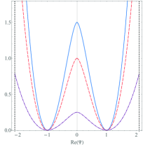
(a) $b<0$

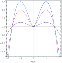
(b) $b>0$

Figure 1: Potential density ${\cal V}(|\Psi|^{2})$ in units of ${n_{c}}$, versus $\text{Re}(\Psi)$ in units of $|\Psi_{e}|=\sqrt{{n_{c}}}$, for these values of $b$: $\pm 3/2$ (solid curve), $\pm 1$ (dashed), $\pm 1/2$ (dash-dotted), given in units of inverse time. Vertical dotted lines represent the condition $|\Psi|\leqslant|\Psi_{\text{cut}}|<\infty$ which is induced by the normalization (2) acting as a constraint.

III Phase Structure

Let us discuss the phase structure of a generic logarithmic fluid described by Eqs. (3) and (2). For simplicity, let us neglect the boundary effects and consider a trapless flow, i.e., $V_{\text{ext}}\equiv 0$. By analogy with Refs. z11appb ; z18zna , by substituting Eq. (1) into (3) and assuming $\textbf{u}=(\hbar/m)\boldsymbol{\nabla}S$ and $\rho=m\,n$, one recovers the hydrodynamic equations for mass and momentum conservation describing a two-phase inviscid fluid with capillarity and internal surface tension:

$$\partial_{t}\rho+\boldsymbol{\nabla}\cdot(\rho\,\textbf{u})=0,$$ (6)

$$\frac{D\textbf{u}}{Dt}\equiv\partial_{t}\textbf{u}+\textbf{u}\cdot\boldsymbol{\nabla}\textbf{u}=\frac{1}{\rho}\boldsymbol{\nabla}\cdot\mathbb{T},$$ (7)

with the stress tensor $\mathbb{T}$ being of the Korteweg form with capillarity ds85 :

$$\mathbb{T}=-\frac{\hbar^{2}}{4m^{2}\rho}\boldsymbol{\nabla}\rho\otimes\boldsymbol{\nabla}\rho-\tilde{p}\,\mathbb{I},$$ (8)

where $\mathbb{I}$ is the identity matrix, $\tilde{p}=p(\rho)-(\hbar/2m)^{2}\boldsymbol{\nabla}^{2}\rho$, and $p(\rho)=-(\hbar b/m)\rho$ is a barotropic equation of state for the pressure $p$.

On the other hand, Eq. (3) can be derived by minimizing an action functional with the following Galilean-invariant Lagrangian density:

$${\cal L}/\hbar=\frac{i}{2}(\Psi\partial_{t}\Psi^{*}-\Psi^{*}\partial_{t}\Psi)+\frac{\hbar}{2m}|\boldsymbol{\nabla}\Psi|^{2}+{\cal V}(|\Psi|^{2}),$$ (9)

with the potential density

$${\cal V}(n)=-bn\left[\ln{(n/{n_{c}})}-1\right]+{\cal V}_{0},$$ (10)

where ${\cal V}_{0}={\cal V}(0)$ is a potential’s shift constant; its value is chosen as to ensure that the function (10) always vanishes at its local minima: ${\cal V}_{0}={n_{c}}(|b|-b)/2$. For complex $\Psi$’s, this potential has nontrivial local extrema at $|\Psi_{e}|=\sqrt{{n_{c}}}$. Correspondingly, they become minima (maxima) if $b$ is negative (positive), as shown in Fig. 1.

These features indicate a symmetry breaking/restoration, and the existence of at least two phases in the fluid. Let us separately study what happens in each of these phases.

III.1 Phase A

When the liquid temperature is above the critical value, $T>T_{c}$, then the nonlinear coupling $b$ is negative, according to (5). The potential density ${\cal V}$ acquires the conventional Mexican hat shape if plotted in a space of real and imaginary parts of $\Psi$, with local degenerate minima located at $|\Psi_{e}|$, see fig. 1a. Therefore, topologically nontrivial solutions exist which interpolate between the local minima z11appb .

Due to separability of Eq. (3) in Cartesian coordinates (which makes it different from other nonlinear wave equations), one can impose the ansatz $\Psi(\textbf{x},t)=\prod\limits_{j=1}^{\bar{d}}\psi_{j}(x_{j},t)$, where $\int_{X_{j}}|\psi_{j}|^{2}dx_{j}=\int_{X_{j}}{\eta}_{j}\,dx_{j}={N}^{1/{\bar{d}}}$, and ${\eta}_{j}=|\psi_{j}|^{2}$ and $X_{j}$ are fluid’s linear density and extent along a $j$th coordinate, respectively.

Then Eq. (3) splits into ${\bar{d}}$ one-dimensional equations:

$$i\partial_{t}\psi_{j}=\left[-\frac{\hbar}{2m}\partial_{x_{j}x_{j}}^{2}+|b|\ln\left(|\psi_{j}|^{2}/{{\eta}_{c}}\right)\right]\psi_{j},$$ (11)

where ${{\eta}_{c}}={n_{c}}^{1/{\bar{d}}}$, and $\partial_{x_{j}}$ is a spatial derivative with respect to $j$th coordinate; a parametric change $b\mapsto-|b|$ is introduced for uniform notations in subsequent formulae. Therefore, in this case we deal with only one 1D differential equation, so the index $j$ can be omitted for brevity.

Furthermore, our solitons are expected to saturate the Bogomolny-Prasad-Sommerfield (BPS) bound Rajaraman:1982is , i.e., obey an equation $d\psi/dx=\pm\sqrt{2\tilde{U}(\psi)},$ where $\tilde{U}(\psi)=(2m|b|/\hbar)\left\{|\psi|^{2}\left[\ln{(|\psi|^{2}/{{\eta}_{c}})}-1\right]+{{\eta}_{c}}\right\}$ is a soliton particle potential, $x\in\{x_{1},...,x_{\bar{d}}\}$, and the sign $\pm$ refers to the soliton and anti-soliton branches. While the analytical solution for this case is unknown, numerical studies reveal the existence of topological solitons of a kink type, see fig. 2. Despite these solutions not being ground-state ones, their longer lifetime is guaranteed by a topological charge, $Q={{\eta}_{c}}^{-1/2}[\psi(+\infty)-\psi(-\infty)]$ which is nonzero for kinks. This separates the topologically nontrivial sector our solitons belong to from the sector with $Q\equiv 0$. The latter has a trivial topology and contains all states with $|\psi|=\text{const}$, including the ground state. Though, in real physical conditions, i.e., in the presence of quantum fluctuations and environment’s influence, these metastable states would eventually decay by emitting waves, which corresponds to a transition to a gas phase.

In a single-soliton setup, these solutions extend for the whole spatial axis, but in a real fluid kinks match with antikinks with periods of order $\ell$. This matching can be visualized by repeating the merged fig. 2 along all spatial directions. According to this figure, the kink soliton’s density increases from its center of mass outwards.

Therefore, a logarithmic fluid in this phase tends to nucleate bubbles with a characteristic size $\ell$, thus forming a foam-like structure, which precedes the process of releasing of vapor or previously dissolved gas, i.e., boiling. If the temperature continues to grow, then boiling eventually occurs, thus indicating a standard vapor-liquid phase transition whose properties can be studied using conventional kinetic theory.

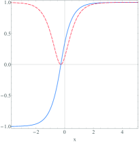
(a) LogSE kink

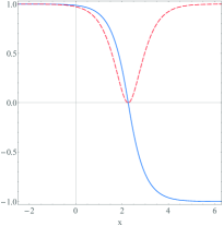
(b) LogSE anti-kink

Figure 2: Profiles of the topological solitons $\psi_{\pm}$ (in units of $\sqrt{{{\eta}_{c}}}$, solid curves) and corresponding densities ${\eta}_{\pm}$ (in units of ${{\eta}_{c}}$, dashed curves), versus the Cartesian coordinate $x$ (in units of $\ell$); the upper (lower) sign corresponds to the kink (anti-kink) solution. For computations we used the boundary condition $\psi(\infty)=\pm\sqrt{{{\eta}_{c}}}$.

III.2 Phase B

When temperature drops below a critical value, $T<T_{c}$, then the nonlinear coupling $b$ turns positive. Therefore, the potential density ${\cal V}$ acquires an upside-down Mexican hat shape if plotted in a space of real and imaginary parts of $\Psi$, with local degenerate maxima located at $|\Psi_{e}|=\sqrt{{n_{c}}}$, see fig. 1b.

For a positive $b$, the ground state solution of Eq. (3) can be found analytically ros68 ; bb76 . It can be written in a form of a Gaussian packet modulated by a plane wave:

$$\Psi_{(g)}(\textbf{x},t)=\pm\sqrt{n_{g}(\textbf{x})}\exp{\left(-i\omega_{g}t\right)},$$ (12)

where

$$n_{g}(\textbf{x}) = \tilde{n}\exp{\left[-\frac{(\textbf{x}-\textbf{x}_{0})^{2}}{\ell^{2}}\right]},$$ (13)

$$\omega_{g} = b\left[{\bar{d}}-\ln{\left(\tilde{n}/{n_{c}}\right)}\right],$$ (14)

where ${\bar{d}}=3$ is a number of spatial dimensions, and $\ell=\sqrt{\hbar/2m|b|}$, $\tilde{n}={N}/\tilde{V}$ and $\tilde{V}=\pi^{{\bar{d}}/2}\ell^{\bar{d}}$ are, respectively, a Gaussian width of the solution, its density’s peak value and its effective volume. The solutions’ profiles are plotted in fig. 3.

The stability of such solutions was confirmed in az11 ; bo15 ; z17zna , therefore in this phase our fluid tends to fragment into a cluster of Gaussian density inhomogeneities, each described by Eq. (13), referred to here as fluid elements. This structure can be visualized by repeating the merged fig. 3 in all directions.

One can treat these elements as point particles of mass $M$ (in general, $M\not=m$), while effectively encoding their nonzero size in the nonlocal two-body interaction potential $\mathbb{U}\left(|\textbf{x}-\textbf{x}^{\prime}|\right)$. In the leading-order approximation, it can be written as

$$\mathbb{U}(r)\approx\frac{U_{0}}{\ell}(r-{\ell_{0}})\,\exp{\left[-(r/\ell)^{2}\right]},$$ (15)

where $r=|\textbf{x}-\textbf{x}^{\prime}|$, $U_{0}$ is the proportionality factor, and $\ell_{0}=\ell\left[1/2+1/(\text{e}\sqrt{\pi}\,\text{erf}(1))\right]+\delta\approx 0.75\ell+\delta$, where $\delta$ being a small parameter responsible for size fluctuations, $\delta\ll\ell$, see Ref. z12eb for further details.

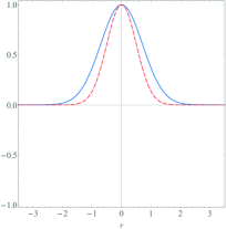
(a) LogSE gausson

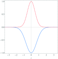
(b) LogSE anti-gausson

Figure 3: Profiles of the Gaussian solitary waves $\Psi_{(g)}(\textbf{x})$, in units of $\sqrt{\tilde{n}}$ (solid curves), and corresponding densities $n_{g}(\textbf{x})$, in units of $\tilde{n}$ (dashed curves), versus the Cartesian axis projected coordinate $r$, in units of $\ell$.

IV Empirical Evidence

In this section, we shall give a brief overview of previous results on logarithmic models’ usage for quantum liquids and dense Bose-Einstein condensates; an emphasis will be given on the experimental evidence existing to date, which supports applicability of these models in the theory of superfluidity of liquid helium.

To begin with, if one assumes that

$$T_{c}\lessapprox T_{\lambda}\approx 2.17\,\text{K}$$ (16)

at normal atmospheric pressure, then the above-mentioned phase structure explains why liquid helium-4 is actively boiling above the $\lambda$-point but remains totally still just under, thus contributing to the effect caused by a jump of heat conductivity.

The logarithmic model analytically describes not only the superfluidity of helium-4, which will be discussed below, but also the phase transition between the foam-like (pre-boiling) and gausson (still) phases, referred to above as phases A  and B, respectively. Strictly speaking, this is an effect, which is separate from the inviscid flow phenomenon per se. It merely states that the formation of bubbles in quantum Bose liquids is a topological effect, which is allowed when the logarithmic nonlinear coupling $b$ is negative, and is forbidden otherwise. In other words, the topological structure of liquid helium changes drastically when crossing the $\lambda$-point. Further above this point, bubble formation eventually leads to the evaporation of the helium, so that the original requirements for a condensate-like material are no longer valid; hence one has to use the methods and notions of the standard kinetic theory.

Furthermore, the above-mentioned Gaussian droplet-like phase is important for understanding the behavior of liquid helium-4 below the $\lambda$-point, historically referred as the helium II phase. In Ref. z12eb , it was shown that this model is very instrumental for describing the superfluid component of helium-4.

For instance, the Landau’s form of an excitation spectrum, i.e., the one which contains a local maximum (“maxon”) followed by a local minimum (“roton”), is a well-known sufficient condition for superfluidity to occur. For helium II, the experimental data coming from neutron scattering put a stringent constraint on a position of both these local extrema, let alone that a candidate model is also expected to reproduce the structure factor curve (coming from X-ray scattering experiments) and speed of sound. Nevertheless, the logarithmic fluid model managed to analytically reproduce with high accuracy three main observable facts of this liquid – Landau spectrum of excitations, structure factor and speed of sound – while using only one non-scale parameter to fit the excitation spectrum’s experimental data.

The resulting theory turned out to be a two-scale model, where the shorter-scale part invoked the wave equation (3), with positive nonlinear coupling, for describing the ground state of the superfluid component of liquid helium and the formation of the effective degrees of freedom called Gaussian fluid elements or parcels. The longer-scale theory picks up from there, deriving the potential (15) as a leading order approximation for interaction between Gaussian elements. It should be emphasized that, while for describing the Landau spectrum the potential (15) is formally sufficient, for describing the structure factor and speed of sound, one needs both this potential and the wave equation (3). This confirms the logarithmic model’s applicability for the superfluid helium phenomenon at different levels.

For superfluid helium-4, the numerical values of the parameters of the two-scale model are

$$b\approx 0.45\,\Delta/\hbar,\ m=m_{\text{He}}\approx 6.64\times 10^{-24}\text{g},$$

$$\ell\approx 1.25\ \text{\AA},\ U_{0}\approx 69\,\Delta,\ M/m\approx 1.23,$$ (17)

where $\Delta\approx 8.65$ K is a “roton” energy gap for helium-4; one can impose that $n_{c}\approx 1/\ell^{3}$ here.

For the phase A, at $T>T_{c}$, the analytical form of interaction potential between the fluid elements is currently unknown. However, one can naturally expect that such a potential belongs to a class of hard-sphere potentials which are popular in the theory of cold quantum liquids psb18 . The common feature of such potentials is that they have a global maximum of repulsive energy at a sphere surface’s radius, and abruptly become zero when moving away from it outwards. This qualitatively resembles behaviour of bubbles which nucleate in superfluid and compose the phase A, as was shown before.

On formal grounds, the logarithmic fluid in this phase is still having a zero viscosity, according to Eq. (7). However, this is different from phase B, because the topological solitons representing the phase-A  bubbles are not ground states of Eq. (3). Instead, they are excited states, although the metastable (or long-lived) ones, due to topological arguments discussed above. This means that phase A  describes a critical superfluid which is just about to boil, i.e., it is an intermediate phase between the phase B  and the phase of active boiling and vaporizing.

Obviously, due to thermal fluctuations, logarithmic superfluid in the vicinity of the critical temperature $T_{c}$ must be a mixture of both phases. Therefore, the statistical mechanical properties of fluid elements of such liquid must be governed by a potential, which is a combination of the potential (15) and a potential of a hard-sphere type.

To conclude, an analytical simplicity of a model together with its good agreement with experiment, clearly indicates that the quantum fluid with logarithmic nonlinearity should be a main component of models of liquid helium at low temperatures. This, of course, does not preclude from using other ingredients, such as the Gross-Pitaevskii condensate (contact two-body interactions, pertinent to weakly-interacting cold gases) and sextic fluid (three-body interactions and Efimov states), which can provide higher-order corrections.

V Additional Force

Until now we have been dealing with an isothermal logarithmic fluid. If, assuming the liquid to be in the phase B, one substitutes a solution (13) into a right-hand side of (7) then it turns out to be zero, which means that the material derivative of the flow’s averaged velocity vanishes. This indicates that inside the ground-state superfluid flow of constant temperature all forces are compensated. What would happen if one introduced a small temperature gradient into the system while keeping its temperature below $T_{c}$?

The simplest way to do so is to recall Eq. (5) and assume that the nonlinear coupling is no longer a constant but a function

$$b=b(\textbf{x},t)\ \Rightarrow\ T=T(\textbf{x},t).$$ (18)

Then the mass conservation equation (6) remains intact, but the momentum equation changes from Eq. (7) to this one:

$$\frac{D\textbf{u}}{Dt}=\frac{1}{\rho}\boldsymbol{\nabla}\cdot\mathbb{T}+\textbf{a},$$ (19)

where the additional acceleration term reads:

$$\textbf{a}=\frac{\hbar}{m}\ln{\!(\rho/\rho_{c})}\,\boldsymbol{\nabla}b(\textbf{x},t),$$ (20)

where $\rho_{c}=m{n_{c}}$. This acceleration looks as if it were caused by an external force $\textbf{f}=\rho\,\textbf{a}$ acting on a fluid parcel, which is parallel to the gradient of $b(\textbf{x},t)$, whence f must be parallel to the temperature gradient, according to Eq. (5).

Let us consider small variations of temperature which do not violate the condition $T<T_{c}$. Using relation (5), formula (20) can be rewritten as

$$\textbf{a}=-\frac{\kappa}{m}\ln{\!(\rho/\rho_{c})}\boldsymbol{\nabla}T\approx-\frac{\kappa}{m}\delta\,\boldsymbol{\nabla}T,$$ (21)

where $\delta=(n-{n_{c}})/{n_{c}}=(\rho-\rho_{c})/\rho_{c}$ is a relative deviation of density from its critical value; the approximation in this equation is valid only if $\delta$ is small. Since $\kappa$ was chosen to be positive by construction, vector a is parallel to the temperature gradient if $\delta<0$, and anti-parallel otherwise.

Let us study a behaviour of that part of force and acceleration, which is related to density only, by re-writing the additional force and acceleration as

$$\textbf{f}=\frac{\kappa}{m}\rho_{c}K_{f}\boldsymbol{\nabla}T,\ \ \textbf{a}=\frac{\kappa}{m}K_{a}\boldsymbol{\nabla}T,$$ (22)

where $K_{f}=-(\rho/\rho_{c})\ln{\!(\rho/\rho_{c})}$ and $K_{a}=-\ln{\!(\rho/\rho_{c})}$ are dimensionless functions of density. Notice that at $\rho\to 0$, vector a does not vanish (moreover, it actually diverges), but the force nevertheless tends to zero. For a fixed value of temperature gradient, it is the function $K_{f}$ which determines a parallel or anti-parallel direction of the force acting on our system, see fig. 4.

One can see that the force changes its direction when density goes across the critical value $\rho_{c}$. Moreover, at densities below $\rho_{c}$ the density-related magnitude of the force has a local maximum, at $\rho\to\rho_{c}/\text{e}$. This can be used for establishing a value of $\rho_{c}$ empirically, without placing superfluid into the critical regime, as well as for searching the conditions under which this force is most visible.

Some concluding remarks are in order here. Firstly, $\rho_{c}$ or ${n_{c}}$ is not necessarily the density of all fluid at $T=T_{c}$. Due to quantum fluctuations, the actual density can be different from this value, let alone that it can be a function of space and time in general. Therefore, ${n_{c}}$ must be treated as a parameter of the logarithmic model, which marks a critical density value at which the logarithmic nonlinearity flips its sign. Secondly, the presented analysis is based on a simplified setup of the irrotational superfluid being free of any external forces and containers (logarithmic fluids in certain types of external potential traps, such as harmonic or Coulomb potentials, were discussed in, e.g., refs. bb76 ; bo15 ; ss18 ). If one considers other physical setups then both the value and direction of this additional acceleration can be different from formula (21), but the fundamental reasons for the effect remain intact.

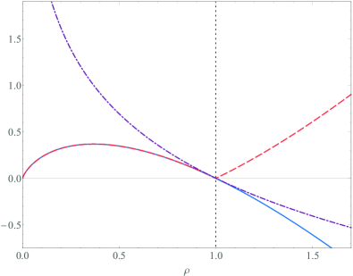
Figure 4: Profiles of dimensionless magnitude functions from Eq. (22), versus density in units of $\rho_{c}$: $K_{f}$ (solid curve), $|K_{f}|$ (dashed curve) and $K_{a}$ (dash-dotted curve).

VI Conclusion

In this paper, we used statistical mechanical arguments to derive an evolution equation for quantum liquid in a condensate-like state, i.e., when average kinetic energies of constituent particles are small compared to the interaction potentials. This equation was shown to contain logarithmic nonlinearity with respect to the condensate function. In the classical hydrodynamics context, this equation can be mapped on the flow of the Korteweg-type materials and diffuse interface models with capillarity and intrinsic surface tension.

The corresponding nonlinear (logarithmic) coupling is shown to be a linear function of the liquid’s temperature. It can take both positive and negative values depending on whether the liquid is, respectively, below or above a critical value. Therefore, the nonlinear coupling’s sign marks two different phases the liquid could be in.

The higher-temperature phase, or phase A in our notations, is characterized by metastable (long-lived) states described by topological solitons with a kink profile, which belong to a topological sector different from the one with the trivial solution. Such solitons can be naturally interpreted as the nucleating bubbles. The foam-like structure which occurs facilitates release of vapor or any gas previously dissolved in the fluid, which is a phase preceding the process of boiling.

The lower-temperature phase, or phase B, is characterized by fluid being in a ground state described by the well-known solution whose density has a Gaussian profile. In a multi-solution picture, this gives rise to a fluid consisting of cell-like inhomogeneities. For such a cellular structure, both an effective interaction potential and many-body Hamiltonian were presented.

It was shown that the logarithmic fluid can be used to model superfluid components of quantum Bose liquids, such as liquid helium-4. The corresponding experimental evidence was discussed.

Furthermore, it turns out that if one introduces a temperature gradient into the logarithmic fluid then the additional force per element arises. This leads to our model being able to predict or explain a number of mechanical phenomena occurring in quantum liquids.

For instance, in the case of superfluid being confined inside a container at a homogeneous gravitational field, at least two temperature gradients usually exist. The first gradient, a horizontal one, occurs when the temperature of the superfluid at its center is slightly different from the temperature on its border adjacent to the container’s walls. The second gradient, a vertical one, occurs along the container’s walls, because the part of a usually non-full container which is in direct contact with superfluid has a slightly different temperature than its rim.

It has been shown that logarithmic superfluid tends to flow along the horizontal gradient of temperature away from a container’s center, as well as along the vertical gradient of temperature between the near-wall parts of superfluid and the container’s rim. This does resemble the known behaviour of liquid helium-4 below the $\lambda$-point: it creeps up to the highest point, which corresponds to an equilibrium between the gravity force, additional force f and molecular bonding with container’s walls, but does not stay there, nor does it return to the inside of its vessel, but instead flows away on the outside wall.

Yet another prediction which follows from our model is that quantum Bose liquids, be it superfluid components of liquified cold gases or Cooper pairs inside superconductors, should affect closely positioned acceleration-measuring devices, such as gyroscopes, which resembles the outcomes of a frame-dragging phenomenon in general relativity (see also remarks about relativistic effects in Sec. II). This becomes possible due to superfluid being a macroscopical yet quantum object, therefore it is not sharply localized within its classical borders. In our model, a wavefunction has a Gaussian “tail”, whereby it can interact with surrounding objects, while the strength of such interaction is determined by the formula (21) or version thereof.

The magnitude of the above-mentioned effects is determined by a product of temperature gradient and density difference $\delta$, on top of a magnitude of the numerical factor $\kappa/m$. Both the temperature gradient and density variations are small in a typical experimental setup eh81 ; gol10arx , which should result in a statistical smallness of the overall effect in the experiments akin to those described in refs. chi82 ; tfc90 ; tps09 ; tp10 . Therefore, in order to achieve a viable effect, it is important to have substantial control over these two parameters.

On the theoretical side, future studies will be devoted to extended models of trapped quantum liquids, which would take into account boundary effects from vessels, rotational dynamics and external potentials, such as harmonic traps or homogeneous gravitational field; those might provide corrections or modifications of the formula (21).

Acknowledgments
I am grateful to participants of the 8th International Conference on Applied Physics and Mathematics ICAPM-2018 in Phuket, Thailand (27-29 January 2018) z18cs1 , and XXIII Fluid Mechanics Conference KKMP-2018 in Zawiercie, Poland (9-12 September 2018) z18cs2 for stimulating discussions and remarks. This work is based on the research supported by the National Research Foundation of South Africa (under Grants Nos. 95965, 98892 and 117769), as well as by the Department of Higher Education and Training of South Africa. Proofreading of the manuscript by P. Stannard is greatly appreciated.

References

- (1) P. L. Kapitsa, Nature 141, 74 (1938).
- (2) J. F. Allen and A. D. Misener, Nature 141, 75 (1938).
- (3) D. R. Tilley and J. Tilley, Superfluidity and Superconductivity (IOP Publishing, Bristol, 1990).
- (4) D. T. Ekholm and R. B. Hallock, J. Low Temp. Phys. 42, 339 (1981).
- (5) V. A. Golovko, arXiv:1103.0517.
- (6) K. G. Zloshchastiev, Grav. Cosmol. 16, 288 (2010).
- (7) K. G. Zloshchastiev, Acta Phys. Polon. 42, 261 (2011).
- (8) A. V. Avdeenkov and K. G. Zloshchastiev, J. Phys. B: At. Mol. Opt. Phys. 44, 195303 (2011).
-
(9)
K. G. Zloshchastiev,
Z. Naturforsch. A 73, 619 (2018).
K. G. Zloshchastiev, arXiv:1906.01816. - (10) S. De Martino, M. Falanga, C. Godano and G. Lauro, Europhys. Lett. 63, 472 (2003).
- (11) G. Lauro, Geophys. Astrophys. Fluid Dyn. 102, 373 (2008).
- (12) G. Lauro, Acta Appl. Math. 132, 405 (2014).
- (13) K. G. Zloshchastiev, Europhys. Lett. (EPL) 122, 39001 (2018).
- (14) J. E. Dunn and J. B. Serrin, Arch. Rat. Mech. Anal. 88, 95 (1985).
- (15) D. M. Anderson, G. B. McFadden and A. A. Wheeler, Annu. Rev. Fluid Mech. 30, 139 (1998).
- (16) T. C. Scott, X. Zhang, R. B. Mann, and G. J. Fee, Phys. Rev. D 93, 084017 (2016).
- (17) Yu. A. Rylov, J. Math. Phys. 40, 256 (1999).
- (18) G. Rosen, J. Math. Phys. 9, 996 (1968).
- (19) I. Bialynicki-Birula and J. Mycielski, Ann. Phys. (N. Y.) 100, 62 (1976).
- (20) J. D. Brasher, Int. J. Theor. Phys. 30, 979 (1991).
- (21) K. G. Zloshchastiev, Eur. Phys. J. B 85, 273 (2012).
- (22) B. Bouharia, Mod. Phys. Lett. B 29, 1450260 (2015).
- (23) K. G. Zloshchastiev, Z. Naturforsch. A 72, 677 (2017).
- (24) R. Rajaraman, Solitons and Instantons (North-Holland, Amsterdam, 1982).
- (25) S. Prestipino, A. Sergi and E. Bruno, Phys. Rev. B 98, 104104 (2018).
- (26) T.C. Scott and J. Shertzer, J. Phys. Commun. 2, 075014 (2018).
- (27) R. Y. Chiao, Phys. Rev. B 25, 1655-1662 (1982).
- (28) J. Tate, S. B. Felch and B. Cabrera, Phys. Rev. B 42, 7885-7893 (1990).
- (29) M. Tajmar, F. Plesescu and B. Seifert, J. Phys.: Conf. Ser. 150, 032101 (2009).
- (30) M. Tajmar and F. Plesescu, AIP Conf. Proc. 1208, 220 (2010).
- (31) K. G. Zloshchastiev, J. Phys.: Conf. Ser. 1039, 012014 (2018).
- (32) K. G. Zloshchastiev, J. Phys.: Conf. Ser. 1101, 012051 (2018).