Nuclear structure uncertainties in coherent elastic neutrino-nucleus scattering

Abstract

The effects of the nuclear structure uncertainties on the description of processes induced by coherent scattering of neutrinos on nuclei are investigated. A reference calculation based on a specific nuclear model is defined and the cross sections and also the expected number of events produced by neutrinos generated by the explosion of a supernova in our galaxy, and by a spallation neutron source are evaluated. By changing the input parameters of the reference calculation their relevance on cross sections and on the number of the detected events is estimated. Seven spherical nuclei with different proton to neutron ratios are considered as possible targets of the neutrinos in the detector, the lightest being ¹²C and the heaviest ²⁰⁸Pb. The effects generated by the uncertainties of the nuclear model are much smaller than those due to the supernova neutrino flux models. This makes the coherent elastic neutrino-nucleus scattering a reliable tool to investigate the details of the neutrino sources, the neutrino-nucleus interaction, and, eventually, also to extract information about neutron distributions in nuclei.

I Introduction

Elastic neutrino scattering processes where the energy of the recoiling nucleus is detected, was proposed some decades ago as an investigation tool for a plethora of conventional neutrino physics topics and new-physics open issues fre74 ; dru84 . Since for neutrinos with energy up to about 100 MeV the individual nucleonic scattering amplitudes overlap in phase bed18 , the process is called Coherent Elastic Neutrino-Nucleus Scattering (CE$\nu$NS) sch15 . Due to its elastic character, there is not a neutrino energy threshold preventing CE$\nu$NS to happen and, thus, for neutrino energies of few tens of MeV, CE$\nu$NS cross sections are remarkably larger than those of other competing processes aki17a ; ric19 ; lin18 . The experimental study of CE$\nu$NS shares various technical problems with direct dark matter searches, therefore many detectors take advantage of the experiences accumulated in this latter investigation field.

The first observation of CE$\nu$NS was reported by the COHERENT collaboration aki17a , making use of the pulsed neutrino emission of the Spallation Neutron Source (SNS) at Oak Ridge National Laboratory. Following this pioneering experience, a remarkable number of new experiments has been planned: CONNIE agu16 , CONUS lin18 , MINER agn17 , $\nu$-gen bel15 , RED-100 aki17b , RICOCHET bil17 , TEXONO won10 NU-CLEUS str17a ; rot19 .

From the theoretical point of view, the main uncertainties in the evaluation of the CE$\nu$NS cross sections come from the proton and neutron density distributions of the target nuclei. Proton density distributions can be obtained from the experimental charge densities extracted from elastic electron scattering data dej87 . Unfortunately, these empirical charge distributions are known only for a limited number of nuclei. Furthermore, one has to consider that the main contribution to CE$\nu$NS cross sections is due to the neutron density distributions which are hardly constrained by experimental data. As a consequence, the information about proton and neutron density distributions is mainly based on nuclear models. In these last years these models have improved a lot their performances in describing nuclear ground states, and, even if formulated in different manners, they show a high degree of agreement in their results co12a .

The present study aims at evaluating the effects of the ambiguities inherent to the description of the proton and neutron distributions on the CE$\nu$NS cross sections. The strategy of our work consists in defining a reference calculation (RC) where a specific nuclear model, which we have developed, tested and perfected in these last years ang14 ; ang15 ; ang16a ; co18a ; ang19 , is used, and then in comparing its results with those of calculations carried out by, reasonably, modifying the input parameters.

A set of nuclei of interest for CE$\nu$NS experiments, and selected in various regions of the nuclear chart, has been investigated. We considered ¹²C, ¹⁶O, ²⁰Ne, ⁴⁰Ar, ⁷⁶Ge, ¹³²Xe and ²⁰⁸Pb. Since our model can be applied only to spherical nuclei, we neglected the slight deformation of the ground states of ¹²C and ²⁰Ne nuclei.

In section II.1, the expressions used to calculate the CE$\nu$NS cross section are shown and related to the proton and neutron density distributions obtained with our model. The details of the nuclear model used to perform the RC are presented in section II.2. Our model has been applied to two specific situations generating neutrinos, and interesting for CE$\nu$NS detection: the case of a supernova explosion in our galaxy, and the neutrino production induced by a spallation neutron source (SNS) sch06 . The information regarding the input parameters needed to estimate the number of detected events expected for these two physical cases is presented in section II.3.

In section III, we study how the CE$\nu$NS cross sections and the number of detected events are modified under various hypotheses about the shape of nuclear form factors. These changes are compared to those induced by the astrophysics uncertainties.

In section IV we summarize the results of our study and conclude that, from the nuclear physics point of view, the CE$\nu$NS processes are well understood. This makes CE$\nu$NS a reliable tool to investigate sources and properties of supernova neutrino fluxes.

II The model

II.1 The CE$\nu$NS cross section

In this section, we present the basic equations describing the elastic scattering of neutrinos off a nucleus. In our expressions we shall use natural units ($\hbar=c=1$). The elastic neutrino scattering process is ruled by weak neutral currents, and we describe them by considering that a single $Z^{0}$ boson is exchanged between the neutrino and the target nucleus. For elastic scattering, in the center of mass reference system, the relation between the neutrino initial and final momenta, ${\bf k}_{i}$ and ${\bf k}_{f}$ respectively, and the neutrino energy $\epsilon_{\nu}$ is

$$|{\bf k}_{i}|=|{\bf k}_{f}|=\epsilon_{\nu}\,.$$ (1)

In the laboratory frame, one has to take into account the recoil of the target, which is zero in the limit of an infinite target mass. Because the nuclear rest masses are much larger than the neutrino energies, the relation (1) is numerically satisfied also in the laboratory frame, therefore the momentum transfer ${\bf q}={\bf k}_{i}-{\bf k}_{f}$ depends only on $\epsilon_{\nu}$ and on the angle $\theta$ between ${\bf k}_{i}$ and ${\bf k}_{f}$, specifically,

$$q^{2}\,=\,({\bf k}_{i}\,-\,{\bf k}_{f})^{2}\,=\,2\,\epsilon_{\nu}^{2}\,(1\,-\,\cos\theta)\,,$$ (2)

where $q=|{\bf q}|$. The recoil energy of the target nucleus can be expressed as

$$T_{\rm rec}\,=\,\frac{q^{2}}{2\,M}\,,$$ (3)

where $M$ indicates the rest mass of the nucleus. For neutrino energies of the order of tens of MeV the nuclear recoil energies are of the order of keV.

We evaluate the cross section by using traditional trace techniques bjo64 , and we obtain, (see eq. (9) of ref. pap15 ),

$$\frac{{\rm d}\sigma}{{\rm d}(\cos\theta)}\,=\,\frac{G_{\rm F}^{2}}{2\,\pi}\,\epsilon_{\nu}^{2}\,(1\,+\,\cos\theta)\,\left|{\cal A}\right|^{2}\,,$$ (4)

where $G_{\rm F}=1.1663787\cdot 10^{-11}\,{\rm MeV}^{-2}$ is the Fermi constant, and ${\cal A}$ the nuclear transition amplitude. In terms of the nuclear recoil energy $T_{\rm rec}$ we obtain the expression,

$$\frac{{\rm d}\sigma}{{\rm d}T_{\rm rec}}\,=\,\frac{G^{2}_{\rm F}\,M}{\pi}\,\left(1\,-\,\frac{M\,T_{\rm rec}}{2\epsilon_{\nu}^{2}}\right)\,\left|{\cal A}\right|^{2}\,.$$ (5)

The nuclear transition amplitude can be expressed as pap15

$${\cal A}\,=\,\left(\frac{1}{2}\,-\,2\,\sin^{2}\theta_{\rm W}\right)\,Z\,F_{\rm p}(q)\,-\,\frac{1}{2}\,N\,F_{\rm n}(q)\,,$$ (6)

where $\theta_{\rm W}$ is the Weinberg angle, with $\sin^{2}\theta_{\rm W}=0.23129$, $Z$ and $N$ are the proton and neutron numbers, respectively, and $F_{\rm p}$ and $F_{\rm n}$ are the proton and neutron nuclear form factors defined as

$$F_{\rm p}(q)\,=\,\frac{4\,\pi}{Z}\displaystyle\int{\rm d}r\,r^{2}\,\frac{\sin(qr)}{qr}\,\rho_{\rm p}^{\rm fold}(r)$$ (7)

and

$$F_{\rm n}(q)\,=\,\frac{4\,\pi}{N}\displaystyle\int{\rm d}r\,r^{2}\,\frac{\sin(qr)}{qr}\,\rho_{\rm n}^{\rm fold}(r)\,.$$ (8)

The proton and neutron, folded, density distributions are normalised to the proton and neutron numbers. In this manner, the value of the nuclear form factors (7) and (8) in the limit for $q\rightarrow 0$ is 1.

An appropriate description of the interaction between the Z⁰ and each nucleon requires to go beyond the approximation where nucleons are assumed to be dimensionless and without internal structure. This is the reason why $F_{\rm p}$ and $F_{\rm n}$ are defined in terms of the corresponding folded density distributions:

$$\rho_{i}^{\rm fold}(r)\,=\,\displaystyle\int{\rm d}r^{\prime}\,\rho_{i}(r\,-\,r^{\prime})\,G^{i}_{\rm w}(r^{\prime})\,=\,\frac{1}{2\,\pi}\,\int\,{\rm d}p\,\exp({i\,p\,r})\,\tilde{\rho}_{i}(p)\,\tilde{G}^{i}_{\rm w}(p)\,,\,\,\,i\equiv{\rm p,n}\,.$$ (9)

Here $\rho_{i}(r)$ is the point-like density distribution and $G^{i}_{\rm w}$ the nucleon weak form factor. Folded densities are actually calculated as indicated in the second equality where $\tilde{\rho}_{i}(p)$ and $\tilde{G}^{i}_{\rm w}(p)$ are the Fourier transforms of the point-like density distribution and of the weak nucleon form factor, respectively.

The isotopic invariance of the strong interactions allows us to connect the nucleonic weak form factor to the electromagnetic one alb02 ; bot04t , therefore

$$\tilde{G}^{i}_{\rm w}(p)\,=\,G_{\rm E}(p)\,,$$ (10)

where $G_{\rm E}(p)$ is the Sachs proton electric form factor. In our calculations we have used the simple dipole parameterization:

$$G_{\rm E}(p)\,=\,\frac{1}{(1\,+\,0.05833\,p^{2})^{2}}\,.$$ (11)

We obtain the total cross section by integrating eq. (4) on $\cos\theta$ or eq. (5) on $T_{\rm rec}$:

$$\sigma\,=\,\displaystyle\int_{-1}^{1}{\rm d}(\cos\theta)\,\frac{{\rm d}\sigma}{{\rm d}(\cos\theta)}\,=\,\int_{0}^{T_{\rm rec}^{\rm max}}{\rm d}T_{\rm rec}\,\frac{{\rm d}\sigma}{{\rm d}T_{\rm rec}}\,.$$ (12)

For a given value of the neutrino energy, $\epsilon_{\nu}$, the maximum value of the target recoil energy is

$$T_{\rm rec}^{\rm max}\,=\,\frac{2\,\epsilon_{\nu}^{2}}{M}\,.$$ (13)

II.2 The nuclear model of the reference calculation

In the calculations of the CE$\nu$NS cross sections, all the information regarding the nuclear target is contained in the proton and neutron form factors that depend only on the nucleon density distributions $\rho_{i}(r)$ of eq. (9). In our RC we use the nucleon distributions obtained with a Hartree-Fock (HF) plus Bardeen-Cooper-Schrieffer (BCS) model that we have developed in these last years ang14 ; ang15 ; ang19 .

As already stated above, the nuclear model used in the present investigation is only valid for spherical nuclei. The solution of the corresponding spherical HF equations rin80 ; suh07 provides a set of single-particle (s.p.) levels characterized by the orbital and total angular momenta, $l$ and $j$ respectively, and the principal quantum number that we label as $n=1,2,\ldots$. The ground state of the nucleus considered is built up by filling separately the various proton and neutron s.p. levels, in ascending order of energy and by taking into account the $2j+1$ degeneracy of each of them.

In the three magic nuclei considered, ¹²C, ¹⁶O and ²⁰⁸Pb, the single particle levels below the Fermi surface are fully occupied. For these nuclei, the role of the pairing is negligible, meaning that its effects on binding and single particle energies, and also on the proton and neutron distributions, are within the numerical accuracy of our calculations.

		protons				neutrons
		s.p. state	$2j+1$	occupancy		s.p. state	$2j+1$	occupancy
20Ne		$1d_{5/2}$	6	2		$1d_{5/2}$	6	2
40Ar		$1d_{3/2}$	4	2		$1f_{7/2}$	8	2
76Ge		$2p_{3/2}$	4	4		$1g_{9/2}$	10	4
132Xe		$2d_{5/2}$	6	4		$1h_{11/2}$	12	8

Table 1: The s.p. Fermi levels for the open shell nuclei considered in the present work. The $2j+1$ column indicates the number of nucleons when the levels are fully occupied. In the column labelled as “occupancy”, we give the number of nucleon occupying the Fermi level for the specific isotope.

In the case of the other nuclei studied, ²⁰Ne, ⁴⁰Ar, ⁷⁶Ge and ¹³²Xe, the s.p. levels with maximum energy are only partially occupied (see table 1) and we carried out HF calculations in the so-called equal filling approximation, that is by considering an average occupancy given by the number of nucleons occupying the level divided by the total occupancy $2j+1$. For these nuclei, the effects of the pairing are not any more negligible and the BCS calculations rin80 ; suh07 , performed on top of the HF ones, permit to take care of them. The RC has been carried out by using an effective nucleon-nucleon finite-range interaction of Gogny type in its D1M parameterization gor09 in both steps of our calculations, the HF and the BCS, where in the latter case it acts as pairing force.

The pairing changes the HF occupation numbers and this modifies the proton and neutron density distributions that, in our model, are obtained as:

$$\rho_{i}(r)\,=\,\sum_{k_{i}}v_{k_{i}}^{2}\,(2j_{k_{i}}+1)\,{\cal R}^{2}_{k_{i}}(r)\,,\,\,\,i\equiv{\rm p,n}\,,$$ (14)

where the index $k_{i}\equiv(n_{k_{i}},l_{k_{i}},j_{k_{i}})$ labels the s.p. state. We have indicated with $v_{k_{i}}^{2}$ its occupation probability and with ${\cal R}_{k_{i}}(r)$ the radial part of its wave function. The sum on ${k_{i}}$ is restricted to proton or neutron states to calculate the respective densities.

We show in table 2 the occupation probabilities obtained in our RC, i.e. HF+BCS with the D1M interaction, for those s.p. states where the differences with the corresponding HF values are larger than 0.01, in absolute value. This occurs only for ⁴⁰Ar, ⁷⁶Ge and ¹³²Xe. In the case of ²⁰Ne this does not happens even if its proton and neutron $1d_{5/2}$ s.p. levels are only partially occupied (see table 1).

		protons				neutrons
		s.p. state	$v_{\rm BCS}^{2}$	$v_{\rm HF}^{2}$		s.p. state	$v_{\rm BCS}^{2}$	$v_{\rm HF}^{2}$
40Ar		$2s_{1/2}$	0.824	1.000		$1d_{3/2}$	0.988	1.000
		$1d_{3/2}$	0.591	0.500
76Ge		$2p_{3/2}$	0.465	1.000		$2p_{1/2}$	0.982	1.000
		$2p_{1/2}$	0.041	0.000		$1f_{5/2}$	0.977	1.000
		$1f_{5/2}$	0.342	0.000		$1g_{9/2}$	0.418	0.400
132Xe		$2d_{5/2}$	0.121	0.670		$3s_{1/2}$	0.972	1.000
		$2d_{3/2}$	0.012	0.000		$2d_{3/2}$	0.940	1.000
		$1g_{7/2}$	0.396	0.000		$1g_{7/2}$	0.981	1.000
		$1h_{11/2}$	0.010	0.000		$1h_{11/2}$	0.705	0.670

Table 2: Occupation probabilities obtained with the D1M interaction in HF+BCS, $v^{2}_{\rm BCS}$, and HF, $v^{2}_{\rm HF}$, calculations for those s.p. levels where the differences are larger than 0.01, in absolute value.

The quality of the nuclear part of the RC in describing experimental observables can be deduced by the results presented in table 3 where we compare the binding energies per nucleon, $B/A$, and the proton and neutron root mean square (rms) radii, calculated as

$$r_{i}\,=\,\left[4\,\pi\,\int{\rm d}r\,r^{4}\,\rho_{i}^{\rm fold}\right]^{1/2}\,,\,\,\,i\equiv{\rm p,n}\,,$$ (15)

with the experimental values bnlw ; ang13 .

The results of table 3 show that the relative differences with the experimental values of both the binding energies and the rms radii, are smaller than 6.5%, in absolute value. The good description of the nuclear binding energies is a test of the validity of the general fit carried out to define the D1M force cha98 . Descriptions of the experimental data of the same quality are obtained by using other parameterizations of the Gogny interaction such as D1S ber91 , D1ST2a gra13 or D1MTd co18a .

		$B/A$ (MeV)				$r_{\rm p}$ (fm)				$r_{\rm n}$ (fm)
		HF+BCS	HFB	exp		HF+BCS	HFB	exp		HF+BCS	HFB
12C		7.246	7.492	7.680		2.544	2.727	2.470		2.526	2.709
16O		7.975	8.000	7.976		2.762	2.934	2.699		2.741	2.911
20Ne		7.508	7.759	8.032		2.951	2.832	3.006		2.911	2.802
40Ar		8.455	8.599	8.595		3.412	3.538	3.427		3.480	3.609
76Ge		8.559	8.648	8.705		4.037	4.153	4.081		4.137	4.276
132Xe		8.327	8.376	8.428		4.765	4.861	4.786		4.861	4.991
208Pb		7.797	7.815	7.867		5.472	5.557	5.501		5.563	5.690

Table 3: Binding energies per nucleon, and proton and neutron rms radii, obtained in the HF+BCS approach with the D1M interaction and in HFB calculations performed with the SLy5 Skyrme force. The experimental values are taken from the compilations of Refs. bnlw and ang13 .

The neutron, $\rho_{\rm n}^{\rm fold}$, and proton, $\rho_{\rm p}^{\rm fold}$, folded densities obtained in the RC are shown in panels (a) and (b) of Fig. 1, respectively. We compare the $\rho_{\rm p}^{\rm fold}$ densities with the empirical charge distributions taken from the compilation of ref. dej87 . The corresponding differences are shown in panel (c) where the largest values, of about 0.015 fm^-3, occur at the nuclear center.

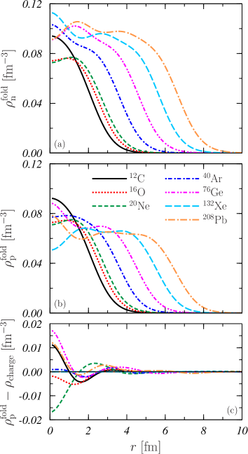
Figure 1: Folded neutron (panel (a)) and proton (panel (b)) densities obtained in the RC according to eq. (9). Panel (c) shows the differences with the empirical charge distributions taken from the compilation of ref. dej87 . In this last panel, the results for ¹³²Xe are not included because the experimental charge density is not available for this nucleus.

The proton and neutron form factors obtained in the RC for all the nuclei considered are shown in Fig. 2. The largest is the nucleus the faster is the decrease towards the first minimum, whose position is located at lower $q$ values.

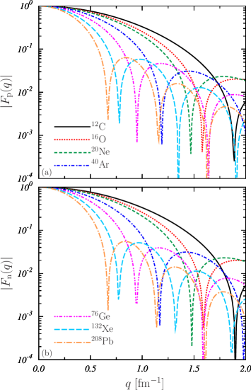
Figure 2: Proton (panel (a)) and neutron (panel (b)) form factors as defined in eq. (7), obtained in the RC for the various nuclei investigated.

The RC total cross sections for the nuclei considered in the present work are presented in Fig. 3. Despite the, expected, quantitative differences, all the curves show analogous behavior. There is a rapid increase of the cross section up to about 30 MeV, then this increase slows down and the cross sections reach a plateau value after $\sim 50\,$MeV. On the other hand the cross sections increase with the atomic number, those of ¹²C being two orders of magnitude smaller than those of ²⁰⁸Pb.

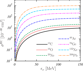
Figure 3: Total cross sections obtained in the RC for all the nuclei considered in the present work.

II.3 Applications

We have used the expression (5) of the differential cross section to estimate the number of events expected for two physical situations. The first one is related to the possibility offered by CE$\nu$NS of detecting neutrinos produced by a supernova explosion in our galaxy. We have assumed the model of supernova cooling described in detail in ref. cos03t . The neutrino emission is characterized by the energy distributions, $f_{\nu_{e}}$ and $f_{\overline{\nu}_{e}}$ of the electron neutrinos, $\nu_{e}$, and antineutrinos, $\overline{\nu}_{e}$, and $f_{\nu_{x}}$ that takes into account the emission of neutrinos and antineutrinos of the other families all together.

The total number of events generated by neutrinos of a given flavour ($\nu_{e}$, $\overline{\nu}_{e}$ or $\nu_{x}$) collected by a detector situated at a distance $D$ from the source, and with a detection threshold energy $E_{\rm th}$ is:

$${\cal N}_{\nu}(E_{\rm th})\,=\,\frac{{\cal I}_{\rm target}\,N_{\nu}}{4\,\pi\,D^{2}}\,\displaystyle\int_{0}^{\infty}{\rm d}\epsilon_{\nu}\,f^{\rm SN}_{\nu}(\epsilon_{\nu})\,\displaystyle\int_{E_{\rm th}}^{T_{\rm rec}^{\rm max}}{\rm d}T_{\rm rec}\,\frac{{\rm d}\sigma}{{\rm d}T_{\rm rec}}\,,$$ (16)

where ${\cal I}_{\rm target}$ indicates the number of target nuclei in the detector,

$$N_{\nu}\,=\,\frac{(1-a_{\rm fl})\,{\cal E}_{B}\,s_{\nu}}{\langle\epsilon_{\nu}\rangle}$$ (17)

is the total number of neutrinos of flavour $\nu$ emitted by the supernova, and $f^{\rm SN}_{\nu}(\epsilon_{\nu})$ the corresponding energy distribution. In the above expression $a_{\rm fl}\simeq 0.01$ indicates the fraction of energy emitted in the neutrino de-leptonization burst, ${\cal E}_{B}$ is the total energy released by the supernova explosion and $s_{\nu}$ is the fraction of these energy carried by each neutrino flavor. Assuming an equal partition of the energy between the different flavours we have $s_{\nu_{e}}=s_{\overline{\nu}_{e}}=1/6$ and $s_{\nu_{x}}=4/6$. Finally,

$$\langle\epsilon_{\nu}\rangle\,=\,\int_{0}^{\infty}{\rm d}\epsilon_{\nu}\,\epsilon_{\nu}\,f^{\rm SN}_{\nu}(\epsilon_{\nu})$$ (18)

is the average neutrino energy.

In the RC we used a recent energy distribution employed in Refs. tam12 ; luj14 and based on a new fit of the numerical simulations of supernovae explosions gal17 :

$$f^{\rm SN}_{\nu}(\epsilon_{\nu})\,=\,{\cal K}\,\frac{\epsilon_{\nu}^{\alpha_{\nu}}\,\exp\left(-\displaystyle\frac{\epsilon_{\nu}}{T_{\nu}}\right)}{\Gamma(\alpha_{\nu}+2)\,T_{\nu}^{\alpha_{\nu}+2}}\,.$$ (19)

In the above equation, $\Gamma(x)$ is the Euler gamma function, and the constant ${\cal K}$ has been inserted to normalize the energy distributions to unity. The values of the parameters $T_{\nu}$ and $\alpha_{\nu}$ for the three neutrino flavors are given in table 4. In this table, we also indicate the average energies, for each neutrino flavor, calculated with eq. (18).

		$f^{\rm SN}_{\nu}(\epsilon_{\nu})$				$f^{\rm MB}_{\nu}(\epsilon_{\nu})$			$f^{\rm FD}_{\nu}(\epsilon_{\nu})$
		$T_{\nu}$ (MeV)	$\alpha_{\nu}$	$\langle\epsilon_{\nu}\rangle$ (MeV)		$T_{\nu}$ (MeV)	$\langle\epsilon_{\nu}\rangle$ (MeV)		$T_{\nu}$ (MeV)	$\eta_{\nu}$	$\langle\epsilon_{\nu}\rangle$ (MeV)
$\nu_{e}$		2.71	2.5	9.49		3.5	10.5		2.5	4.0	11.17
$\overline{\nu}_{e}$		3.43	2.5	12.01		5.0	15.0		3.6	2.0	12.98
$\nu_{x}$		4.46	2.5	15.61		8.0	24.0		4.8	1.0	15.96

Table 4: Parameters used in the expressions of the supernova neutrino energy distributions (19), (30) and (31) taken from Refs. pap15 ; gal17 . The corresponding average energy values $\langle\epsilon_{\nu}\rangle$ are also shown.

In the RC we considered the neutrinos emitted by a supernova which releases a total energy of ${\cal E}_{B}=3.0\times 10^{53}\,$erg at a distance $D=10\,$kpc from the earth laboratory where a $1\,$t detector is used.

The second application of our model is related to the production of neutrinos induced by a SNS. In a first step the neutrons generated by the source interact with a nuclear target and produce $\pi^{+}$ pions. By stopping these pions we obtain monochromatic neutrinos from the decay of $\pi^{+}$ at rest:

$$\pi^{+}\,\rightarrow\,\mu^{+}\,+\,\nu_{\mu}\,.$$ (20)

These are the prompt, monochromatic, neutrinos whose energy distribution is

$$f^{\rm SNS}_{\nu_{\mu}}(\epsilon_{\nu_{\mu}})\,=\,\delta(\epsilon_{\nu_{\mu}}\,-\,E_{\nu_{\mu}})$$ (21)

where

$$E_{\nu_{\mu}}\,=\,\frac{m^{2}_{\pi}\,-\,m^{2}_{\mu}}{2\,m_{\pi}}\,=\,29.79\,{\rm MeV}\,.$$ (22)

In the previous expression, we have indicated with $m_{\pi}$ and $m_{\mu}$ the pion and muon mass, respectively. We neglect the tiny fraction of electron neutrinos coming from the $\pi^{+}$ decay.

In addition to the prompt neutrinos, there are also the delayed neutrinos coming from the decay of $\mu^{+}$:

$$\mu^{+}\,\rightarrow\,e^{+}\,+\,\overline{\nu}_{\mu}\,+\,\nu_{e}\,.$$ (23)

The energy distributions of this three-body decay are well described as avi03 :

$$f^{\rm SNS}_{\nu_{e}}(\epsilon_{\nu_{e}}) = \frac{96\,\epsilon^{2}_{\nu_{e}}}{m_{\mu}^{4}}\,\left(m_{\mu}\,-\,2\,\epsilon_{\nu_{e}}\right)\,\theta\left(\epsilon_{\nu_{e}}\,-\,\frac{m_{\mu}}{2}\right)\,,$$ (24)

$$f^{\rm SNS}_{\overline{\nu}_{\mu}}(\epsilon_{\overline{\nu}_{\mu}}) = \frac{16\,\epsilon^{2}_{\overline{\nu}_{\mu}}}{m_{\mu}^{4}}\,\left(3\,m_{\mu}\,-\,4\epsilon_{\overline{\nu}_{\mu}}\right)\,\theta\left(\epsilon_{\overline{\nu}_{\mu}}\,-\,\frac{m_{\mu}}{2}\right)\,,$$ (25)

where $\theta(x)$ is the step, or Heaviside, function.

The total number of events generated by neutrinos of a given flavour and collected by a detector with a threshold energy $E_{\rm th}$, is given by

$${\cal N}_{\nu}(E_{\rm th})\,=\,\Phi\,{\cal I}_{\rm target}\,t\,\,\displaystyle\int_{0}^{\infty}{\rm d}\epsilon_{\nu}\,f^{\rm SNS}_{\nu}(\epsilon_{\nu})\,\displaystyle\int_{E_{\rm th}}^{T_{\rm rec}^{\rm max}}{\rm d}T_{\rm rec}\,\frac{{\rm d}\sigma}{{\rm d}T_{\rm rec}}\,,$$ (26)

where we have indicated with $\Phi$ the neutrino flux reaching the detector and with $t$ the exposure time.

In the case of the SNS, for the RC, we have assumed a detection time of one year with a detector of $1\,$t situated at a distance from the source such as it can receive a flux of $10^{7}\,$neutrinos per cm² in one second.

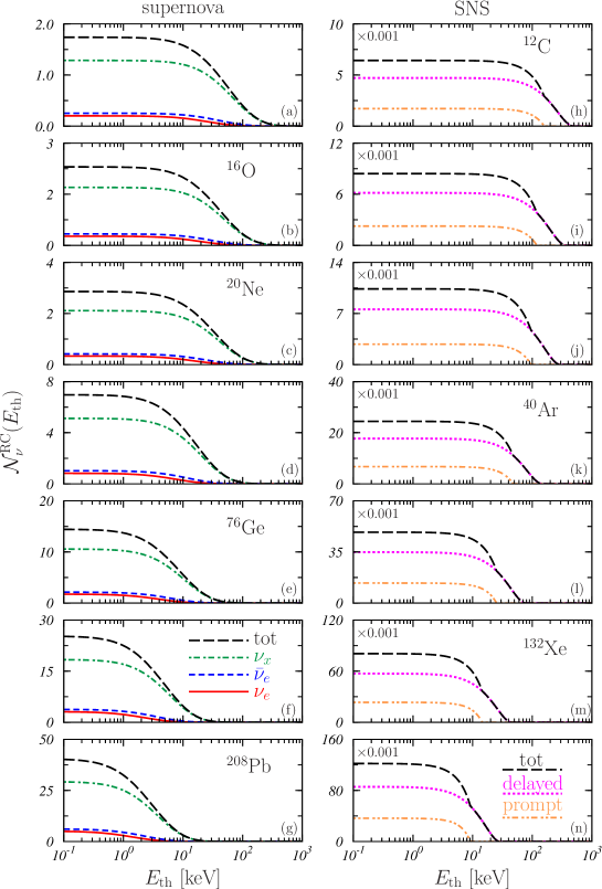
Figure 4: Number of detected events obtained in the RC as a function of the detection threshold energy for the cases of supernova explosion (left-handed panels) and SNS (right-handed panels), according to Eqs. (16) and (26), respectively. Each couple of aligned panels shows the results obtained for a specific target nucleus. In the left-handed panels, solid red, dashed blue and dashed-dotted green curves correspond to $\nu_{e}$, $\bar{\nu}_{e}$ and $\nu_{x}$, respectively. In the right-handed panels, the dotted pink and dashed double-dotted orange curves show the contributions of delayed and prompt neutrinos, respectively. All the values of the SNS results have been divided by 1000. In both supernova and SNS cases, the long-dashed black curves indicate the total number of events.

In Fig. 4 the number of events obtained in the RC are shown as a function of the detection threshold energy $E_{\rm th}$. The results of the left panels (a-g) correspond to the supernova explosion, eq. (16), while those of the right panels (h-n) have been obtained for the SNS, eq. (26). Each couple of aligned panels presents results for the same target nucleus. In each panel, the dashed black curve indicates the total number of events, calculated as

$${\cal N}(E_{\rm th})\,=\,\sum_{\nu}{\cal N}_{\nu}(E_{\rm th})\,,$$ (27)

where the sum runs over the three flavors considered in each case, $\nu_{e}$, $\overline{\nu}_{e}$ and $\nu_{x}$ for the supernova, and $\nu_{\mu}$, $\nu_{e}$ and $\overline{\nu}_{\mu}$ for the SNS. In the figure, all the SNS results are divided by a factor 1000.

As expected, in both cases, the number of events increases with the mass number of the target nucleus and with the lowering of the detection threshold energy $E_{\rm th}$. At the lowest value of $E_{\rm th}$ we have considered, $10^{-1}$ keV, the number of the expected events in ²⁰⁸Pb is 20 times larger than in ¹²C. On the other hand, light nuclei extend their sensitivity at higher values of $E_{\rm th}$. The value of the detection threshold energy at which ${\cal N}(E_{\rm th})=0$ in ¹²C is about one order of magnitude larger than in ²⁰⁸Pb.

In the case of supernova neutrinos, the smallest contribution is given by $\nu_{e}$, solid red curves, while the largest one is due to $\nu_{x}$, dashed-dotted green curves. The contribution of $\overline{\nu}_{e}$ (short dashed blue curves) is similar to that of $\nu_{e}$. The main reason for this result is that all the neutrino flavors other than electron neutrinos and antineutrinos are summed up on the $\nu_{x}$ contribution and this collective contribution is weighted 4/6, while that of $\nu_{e}$ and $\overline{\nu}_{e}$ count 1/6 each.

For the SNS neutrinos, we separately show the contribution of the prompt neutrinos, dashed double-dotted orange curves, and that of the delayed ones, dotted violet lines, which is about two times larger than the previous one. This is mainly due to the fact that there are two delayed neutrino flavors, $\nu_{e}$ and $\overline{\nu}_{\mu}$, while the prompt neutrinos are only $\nu_{\mu}$.

III Comparison with the reference calculation

As already pointed out in the introduction, the strategy of our investigation consists in comparing the results of the RC with those obtained by changing some of the reference inputs. This comparison will be done by considering mainly the total cross section, $\sigma(\epsilon_{\nu})$, and the total number of events, ${\cal N}(E_{\rm th})$. For this reason, we have considered two quantities which emphasize the differences between the results of both calculations. For the total cross section, given by eq. (12), we have used the absolute value of the corresponding relative difference:

$$\Delta\sigma(\epsilon_{\nu})\,=\,\frac{\left|\sigma(\epsilon_{\nu})\,-\,\sigma^{\rm RC}(\epsilon_{\nu})\right|}{\sigma^{\rm RC}(\epsilon_{\nu})}\,.$$ (28)

Here $\sigma(\epsilon_{\nu})$ refers to the new calculation. For the total number of events, defined in eq. (27), we have calculated:

$$\Delta{\cal N}(E_{\rm th})\,=\,\frac{\left|{\cal N}(E_{\rm th})\,-\,{\cal N}^{\rm RC}\,(E_{\rm th})\right|}{{\cal N}^{\rm RC}\,(E_{\rm th}=0)}\,,$$ (29)

a quantity normalized to the maximum total number of events obtained in the RC, ${\cal N}^{\rm RC}\,(E_{\rm th}=0)$.

III.1 The nuclear form factors

If one assumes the low-$q$ limit of the form factors by setting $F_{\rm p}(q)=F_{\rm n}(q)=1$, the transition amplitude ${\cal A}$, eq. (6), depends only on the proton and neutron numbers, $Z$ and $N$ respectively, and the total cross section (12) increases as $\epsilon_{\nu}^{2}$. This can be observed in Fig. 6(a) where the relative differences $\Delta\sigma$, defined in eq. (28), are shown for all the nuclei studied as a function of $\epsilon_{\nu}$. As it can be seen, $\Delta\sigma$ increases with the nuclear mass.

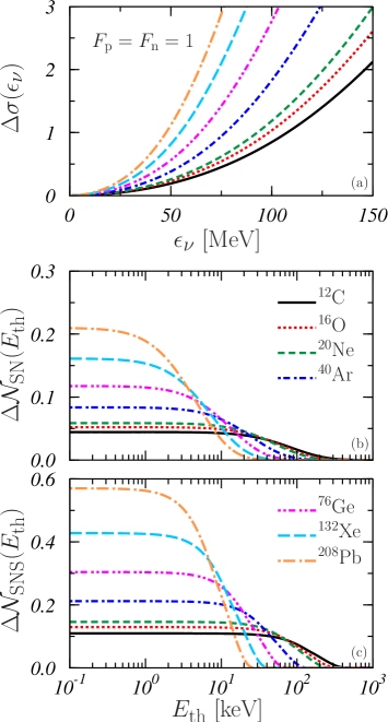
Figure 5: Relative differences $\Delta\sigma$ (panel (a)), defined in eq. (28), and $\Delta{\cal N}$, defined in eq. (29), for supernova (panel (b)) and SNS (panel (c)), obtained by making $F_{\rm p}=F_{\rm n}=1$ in the RC.

Figure 6: Same as in Fig. 6 but for $F_{\rm p}=0$.

The effects of this approximation on the number of events are shown in panels (b) and (c) of Fig. 6 where we present the values of $\Delta{\cal N}$, eq. (29) for supernova and SNS neutrinos, respectively, as a function of $E_{\rm th}$. Despite the quadratic increase of the cross section with the neutrino energy, the total number of events is limited in both cases. This is due to the neutrino energy distributions which impose a maximum value of $\epsilon_{\nu}$; specifically, about $50\,$MeV in the case of the supernova (see below), and $m_{\mu}/2$, in the case of SNS (see Eqs. (24) and (25)).

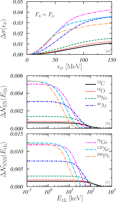
Figure 7: Same as in Fig. 6 but for $F_{\rm n}=F_{\rm p}$.

According to eq. (6), the proton contribution to the transition amplitude is multiplied by a factor containing the Weinberg angle, whose value is about 0.037. This implies that the contribution of the protons to the CE$\nu$NS cross section is strongly suppressed, and the process is mainly sensitive to the neutron density distribution. The relevance of the proton distribution can be deduced from Fig. 6, where the quantities $\Delta\sigma$ and $\Delta{\cal N}$, for supernova and SNS, calculated by setting $F_{\rm p}=0$, are shown.

As it can be seen in panel (a), the values of $\Delta\sigma$ are almost independent of $\epsilon_{\nu}$ and coincide for the three nuclei with $N=Z$. For the other nuclei we have considered, where $N>Z$, the contribution of the protons becomes smaller and, consequently, the values of $\Delta\sigma$ reduce. As expected, the lowest value is that of ²⁰⁸Pb, the nucleus with the largest difference between neutron and proton numbers.

The consequences of neglecting the proton contribution on the detected number of events, are shown in panels (b) and (c) of Fig. 6. The results for supernova and SNS neutrinos are very similar. The behavior of $\Delta{\cal N}$ follows that of $\Delta\sigma$. For the nuclei with $N=Z$ we obtained similar values of $\Delta{\cal N}$, about 17% at $E_{\rm th}=0.1\,$keV. For the other nuclei this value becomes smaller as $N-Z$ increases until a minimum of $\sim 10\%$ is reached in ²⁰⁸Pb.

The results of Fig. 2 show that there are not large differences between the proton and neutron nuclear form factors used in the RC. Since the charge distributions are known for a remarkable number of nuclei dej87 , one could use these empirical distributions also for neutrons. We have carried out calculations where we substitute the neutron form factors with those of the protons. The results obtained are compared with those of the RC in Fig. 7.

In this case, the values of $\Delta\sigma$ and $\Delta{\cal N}$ are much smaller than those presented in the previous two figures. The behavior of $\Delta\sigma$ shows an increase with $\epsilon_{\nu}$. This is because the larger is the neutrino energy, the larger becomes the value of the momentum transfer, and, therefore, the differences between the form factors are more relevant.

The consequences of using the same form factors for protons and neutrons on ${\cal N}$ are very small in comparison with those we have previously discussed. In general, $\Delta{\cal N}$ grows with $A$ at low $E_{\rm th}$, and reaches a value of about 0.5% for ⁷⁶Ge, ¹³²Xe and ²⁰⁸Pb nuclei in the case of the supernova and roughly the double in SNS.

In the interaction between neutrino and nucleons we considered the weak form factor of each nucleon defined in eq. (10) to generate the folded nucleon densities according to eq. (9). The differences between the point-like distributions generated in our HF+BCS nuclear model and those obtained after the folding with the nucleonic form factor are shown in Fig. 9. The effects of this folding are more relevant at the nuclear interior where they reach $\sim 15\%$ of the maximum density values in some of the nuclei studied. We have also considered parameterizations of the nucleonic form factor different from that used in our RC (see eq. (11)), but the changes in the folded density distributions are within the numerical accuracy of our calculations.

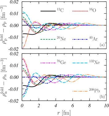
Figure 8: Differences between folded and point-like density distributions for the nuclei considered in the present work. Protons (panel (a)) and neutrons (panel (b)) results are shown.

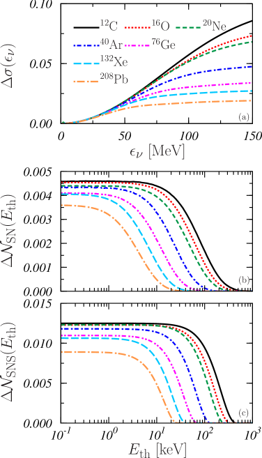
Figure 9: Relative differences $\Delta\sigma$ and $\Delta{\cal N}$ between results obtained by using point-like and folded densities.

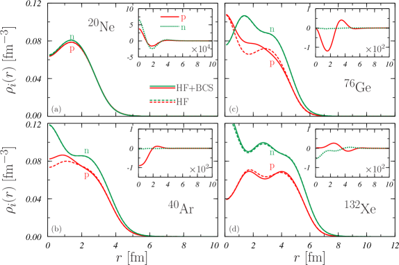
Figure 10: Proton (red curves) and neutron (green curves) point-like densities obtained according to eq. (14). HF densities (dashed curves) are compared to the HF+BCS ones (full lines), for those nuclei with s.p. levels not fully occupied. The insets show the differences between the two distributions.

The differences between the RC results and those obtained by using the point-like nucleon distributions are presented in Fig. 9. The results shown in panel (a) indicate that, at high $\epsilon_{\nu}$, $\Delta\sigma$ reaches values of about $10\%$ in ¹²C and 2% in ²⁰⁸Pb. We show in panels (b) and (c) the values of $\Delta{\cal N}$ for supernova and SNS. In both cases these differences are very small, 0.5% at most in the former case and 1.5% in the latter one.

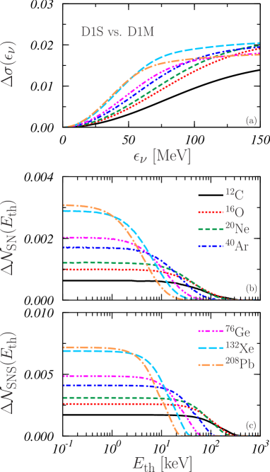
Figure 11: Relative differences $\Delta\sigma$ and $\Delta{\cal N}$ corresponding to the results obtained by using the D1S interaction instead of the D1M in the RC.

III.2 The nuclear models

In this section, we study the impact on the quantities of interest for CE$\nu$NS processes of the uncertainties related to the various hypotheses used in developing the nuclear model.

We consider first the effect of the pairing on the proton and neutron distributions. In Fig. 10, the point-like HF densities (dashed lines) are compared with the point-like densities obtained in a HF+BCS calculation (full lines). We have considered here the four nuclei with open shells where pairing effects are expected to be more relevant. However, the figure clearly shows that the differences between the densities obtained in both calculations are very small, and their effects on the cross sections and on the number of the detected events are within the numerical accuracy of our calculations.

Another source of uncertainty in the nuclear model is related to the effective nucleon-nucleon interaction. We compare the results of our RC with those obtained by carrying out the same HF+BCS calculations with a different effective nucleon-nucleon interaction. In these latter calculations we have used the D1S parameterization of the Gogny interaction ber91 instead of the D1M used in our RC. The effects on the total cross sections and on the number of detected events are shown in Fig. 11. The differences in the total cross sections are below 2% while in the total number of events they are smaller than 0.3%, in the case of the supernova, and 0.8%, in the case of the SNS.

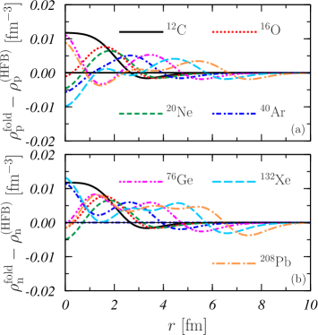
Figure 12: Differences between the proton, panel (a), and neutron, panel (b), folded densities used in our RC and those obtained in HFB calculations with the SLy5 force.

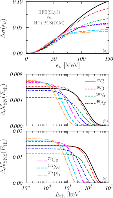
Figure 13: Relative differences $\Delta\sigma$ and $\Delta{\cal N}$ corresponding to the results obtained by using the nucleon distributions obtained in a HFB calculation with the SLy5 Skyrme interaction instead of those considered in the RC.

An additional test of the reliability of our RC has been done by making a comparison with the results of Hartree-Fock-Bogolioubov (HFB) calculations performed with the SLy5 Skyrme interaction. We have carried out these latter calculations with the HFBRAD code ben05 . As it usually occurs in HFB when a zero-range effective nucleon-nucleon interaction is used in the HF sector, the force considered in the pairing sector is not the same. In our case, we have used a so-called volume pairing field that follows the density shape (see ref. ben05 for details).

The quality of these HFB calculations in describing the empirical values of binding energies and rms charge radii is indicated in table 3. We observe that the performances are rather similar to those of our RC calculations.

We show in Fig. 13 the differences between the folded densities calculated within our RC and those obtained in the HFB approach. The largest differences are located at the center of the nuclei and they are about the 10% of the maximum values of the densities.

The effects of these differences on the cross sections and on the number of detected events are shown in Fig. 13. Even though $\Delta\sigma$ reaches values up to about 10% (in the case of ¹²C and for $\epsilon_{\nu}$=150 MeV), the differences $\Delta{\cal N}$ are below 0.8% and 2% for the supernova and SNS, respectively.

Our work is based on the assumption that our model, describing well the experimental values of binding energies, charge radii and distributions, provides also a good description of the, experimentally unknown, neutron densities. The recent measurements of the PREX collaboration PREX12 indicates, for the ²⁰⁸Pb nucleus a neutron radius of $r_{\rm n}=5.78^{+0.16}_{-0.18}\,$fm, slightly larger than the value of $5.563\,$fm of our RC (see table 3). Also the estimate of Horowitz et al. Hor12 , $r_{\rm n}=5.751\pm 0.175({\rm exp})\pm 0.026({\rm model})\pm 0.005({\rm strange})\,$fm, is larger than our RC result. The value of $r_{\rm n}$ measured by the PREX collaboration for ²⁰⁸Pb is an open problem, since it is remarkably larger than values obtained with a variety of experimental procedures which are closer to our RC result Kra13 .

Despite the fact that the difference between the PREX result and those obtained with other techniques has not yet been clarified, we have considered the effects generated by a neutron density larger than that of our RC. For this purpose, we have rescaled our RC neutron density to generate a new $\rho^{\rm fold}_{\rm n}$ with $r_{\rm n}=5.780\,$fm. In panel (a) of Fig. 14 we compare the new density with that obtained in our RC. We calculated the total cross section and the total number of events for supernova and SNS with the rescaled neutron density. The relative differences with respect to the RC results are shown in panels (b) and (c) of this figure.

We observe a maximum value of $\Delta\sigma$ of about 8% at $\epsilon_{\nu}$ = 150 MeV, and values of about 3% for $\Delta{\cal N}$ in the SNS case, and even smaller, 1.5%, for the supernova case. These values are of the same order of magnitude of those obtained by setting $F_{\rm n}=F_{\rm p}$ (see Fig. 7) or by using the D1S interaction instead than the D1M (see Fig. 11).

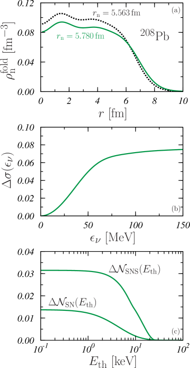
Figure 14: Effects of the consideration of an enlarged neutron density for ²⁰⁸Pb. In panel (a) this density (green solid curve) is compared to that used in the RC (black dotted curves). Panel (b) and (c) show the relative difference differences $\Delta\sigma$ and $\Delta{\cal N}$ obtained for the enlarged neutron density.

III.3 Uncertainties on neutrino sources

The aim of our work is to evaluate the robustness of our RC in the evaluation of the CE$\nu$NS cross sections, in order to asses its reliability in the investigation of the supernova neutrino sources. In the previous sections we have analyzed how the uncertainties on the various inputs of our nuclear model affect the cross sections and the number of detected events in the cases of a supernova explosion and the SNS.

One of the main goals of the neutrino detection of an eventual supernova explosion in our galaxy is to identify the temperature and the average energy related to the energy distribution. This would provide important information on the explosion mechanism and the cooling phase. Therefore, we study now how the number of detected events is sensitive to one of the major uncertainties related to the supernova neutrino models in that case: the energy distribution of the neutrino flux.

In our RC, the neutrino energy distribution considered for the case of the supernova explosion is the $f^{\rm SN}_{\nu}$ defined in eq. (19). There are various plausible alternatives, and among them we have selected a Maxwell-Boltzmann distribution gio06 ; pap15 ,

$$f^{\rm MB}_{\nu}(\epsilon_{\nu})\,=\,\frac{\epsilon_{\nu}^{2}}{2\,T_{\nu}^{3}}\,\exp\left(-\,\displaystyle\frac{\epsilon_{\nu}}{T_{\nu}}\right)\,,$$ (30)

and a Fermi-Dirac like distribution pag09 ,

$$f^{\rm FD}_{\nu}(\epsilon_{\nu})\,=\,{\cal C}\,\frac{\epsilon_{\nu}^{2}}{1\,+\,\exp\left(\displaystyle\frac{\epsilon_{\nu}}{T_{\nu}}\,-\,\eta_{\nu}\right)}\,.$$ (31)

Here ${\cal C}$ is a constant included to normalize to unity the integral of the distribution. The values of $T_{\nu}$ and $\eta_{\nu}$ for each neutrino type and the average neutrino energies are given in table 4.

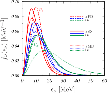
Figure 15: Energy distributions of the neutrino emitted by a supernova. The red curves indicate $\nu_{e}$, the blue curves $\overline{\nu}_{e}$ and the green curves $\nu_{x}$. Dotted, dashed and solid curves correspond to the $f^{\rm MB}_{\nu}$, $f^{\rm FD}_{\nu}$ and $f^{\rm SN}_{\nu}$ distributions as given by Eqs. (30), (31) and (19), respectively. The parameters shown in table 4 have been used.

In Fig. 15 we show the behavior of these energy distributions for the three neutrino flavors. The most remarkable result is the large difference between $f_{\nu}^{\rm MB}$ and the other two distributions, in the case of $\nu_{x}$. In this latter case, the distribution is still relatively large for neutrino energies above 40 MeV, where all the other distributions are negligible.

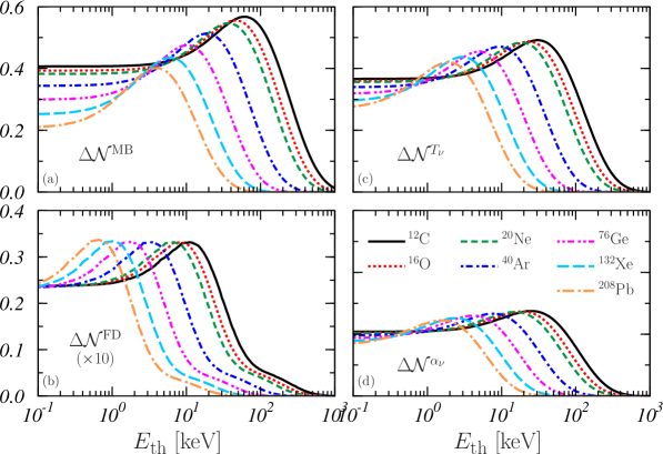
Figure 16: Relative differences $\Delta{\cal N}$ between the number of events from supernova explosion obtained by changing the neutrino energy distribution. In panel (a) we show the results obtained by using the Boltzmann energy distribution eq. (30). In panel (b) those found for the Fermi-like energy distribution of eq. (31). The differences shown in panel (c) and (d) are defined in eq. (32) and correspond to varying by $\pm 20\%$ the values of the parameters $T_{\nu}$ and $\alpha_{\nu}$ of $f$ given in table 4. Note that the values of the panel (b) are multiplied by 10.

In panels (a) and (b) of Fig. 16 we show the relative differences $\Delta{\cal N}$ between the results obtained by using $f^{\rm MB}_{\nu}$ and $f^{\rm FD}_{\nu}$ instead of $f^{\rm SN}_{\nu}$ in the RC. These differences are remarkable larger than those obtained by changing the nuclear physics inputs (compare with the analogous results shown in Figs. 11 and 13).

The calculations done with $f^{\rm FD}_{\nu}$ (panel (b)) produce differences $\Delta{\cal N}^{\rm FD}$ up to about 3.5% (the results in the figure are multiplied by a factor 10). The values of $\Delta{\cal N}^{\rm MB}$ (panel (a)) are much larger at the maximum, ranging from about $40\%$ in ²⁰⁸Pb up to roughly $60\%$ in ¹²C. We expected such large values because of the strong differences between $f^{\rm SN}_{\nu}$ and $f^{\rm MB}_{\nu}$ observed in Fig. 15.

We further estimate the sensitivity of our results to the neutrino energy distributions by carrying out calculations with different values of the $T_{\nu}$ or $\alpha_{\nu}$ parameters in the $f_{\nu}$ energy distribution. In panels (c) and (d) of Fig. 16 we show the relative differences

$$\Delta{\cal N}^{\lambda}(E_{\rm th})\,=\,\frac{{\cal N}^{\lambda+}(E_{\rm th})\,-\,{\cal N}^{\lambda-}(E_{\rm th})}{{\cal N}^{\rm RC}(E_{\rm th}=0)}\,,\,\,\,\lambda\equiv{T_{\nu},\alpha_{\nu}}\,,$$ (32)

where ${\cal N}^{\lambda+}$ and ${\cal N}^{\lambda-}$ indicate the total number of events obtained by increasing and reducing the parameter $\lambda$ ($T_{\nu}$ or $\alpha_{\nu}$) by 20%, respectively.

The values of $\Delta{\cal N}^{T_{\nu}}$ are larger than those of $\Delta{\cal N}^{\alpha_{\nu}}$ and they are of the same order as the differences found when $f^{\rm MB}_{\nu}$ is used instead of $f^{\rm SN}_{\nu}$ in the RC. In the peak $\Delta{\cal N}^{T_{\nu}}$ varies between $\sim 50\%$, in ¹²C, and $\sim 40\%$, in ²⁰⁸Pb, whereas $\Delta{\cal N}^{\alpha_{\nu}}$ is below 20% in all nuclei considered.

IV Summary and conclusions

The aim of our work was to investigate the effects on CE$\nu$NS generated by the uncertainties on the description of the nuclei which are the target of the neutrinos. The evaluation of the CE$\nu$NS cross section requires the knowledge of the proton and neutron density distributions of the target nucleus. We defined a type of calculation, which we called RC, containing reasonable, and up to date, ingredients for a description of the nuclear ground state. The obtained CE$\nu$NS cross sections were used to study two specific physical situations: the detection of neutrinos coming from supernova explosions and those from SNS. We evaluated the expected number of detected events for these two cases by considering an ideal detector and some specific characteristics of the incoming neutrino fluxes. Our working strategy consisted in modifying the various inputs of the RC and then by comparing the new results with those of RC.

We first pointed out the importance of the role of the nucleon form factors, defined as the Fourier transform of the proton and neutron distributions. If the low-$q$ limit is considered, $F_{\rm p}=F_{\rm n}=1$ and, though the CE$\nu$NS cross section rises as $\epsilon_{\nu}^{2}$, the number of the detected events is limited since the neutrino energy distributions have a maximum energy. In this situation the differences with respect to the RC results are rather large arriving at about 60% for SNS neutrino with ²⁰⁸Pb  target.

The main contribution to the CE$\nu$NS is provided by the neutrons, however, the presence of the protons is not negligible. We found that, if $F_{\rm p}$ is neglected, the effects produced are worth up to 15% in $N=Z$ nuclei. Clearly, for nuclei with neutron excess the effect becomes smaller, even though it is always larger than 10%.

These two basic requirements of the calculation are those producing the largest effects. We studied the use of the same form factors for protons and neutrons, the role of the weak nucleonic form factor, that of the pairing, that of the effective nucleon-nucleon interaction, and that of an alternative nuclear structure model. In the case of the ²⁰⁸Pb nucleus, we have also investigated the effects produced by a rescaling of the neutron distribution to obtain larger rms radius. All these changes, with respect to our RC, generate effects that are, at least, one order of magnitude smaller than those produced in the two cases quoted above. We are talking about effects of the order of few percents.

We compared these tiny effects due to the nuclear structure with those related to the uncertainties on the supernova neutrino flux models. Specifically, we concentrated on the energy distributions of the neutrino emitted by a supernova. First we adopted two, reasonable, energy distributions different from to that used in our RC. In a second step we modify by 20% the parameters of the energy distributions used in the RC. These changes of the neutrino energy distributions produce effects of about 10%, at least one order of magnitude larger than those induced by the nuclear structure uncertainties. Our results agree with those obtained using other simpler, analytical, nucleon densities and/or form factors pap15 ; Ari19 .

We conclude that CE$\nu$NS processes can be reliably used to study the details of the neutrino sources generated by a supernova explosion, since the nuclear structure uncertainties generate effects orders of magnitude smaller than those related to the neutrino emission.

On the other hand, the use of CE$\nu$NS experiments to get information on the neutron distribution, as it has been recently envisaged pat12 ; cad18 ; ciu18 ; Pay19 , requires a knowledge of the neutrino flux of few percent.

References

- (1) D. Z. Freeman, Coherent effects of a weak neutral current, Phys Rev. D 9 (1974) 1389.
- (2) A. Drukier, L. Stodolsky, Principles and applications of a neutral-current detector for neutrino physics and astronomy, Phys Rev. D 30 (1984) 2295.
- (3) V. A. Bednyakov, D. V. Naumov, Coherency and incoherency in neutrino-nucleus elastic and inelastic scattering, Phys. Rev. D 98 (2018) 053004.
- (4) K. Scholberg, Coherent elastic neutrino-nucleus scattering, J. Phys. G Conference Series 606 (2015) 012010.
- (5) D. Y. Akimov, et al., Observation of coherent elastic neutrino-nucleus scattering, Science 357 (2017) 1123.
- (6) G. C. Rich, Coherent elastic neutrino-nucleus scattering, Proceedings of Science NOW 2018 (2019) 084.
- (7) M. Lindner, New neutrino states and interactions 2018. Talk at NOW 2018, http://www.ba.infn.it/ now/now2018/assets/lindner-now2018.pdf.
- (8) A. Aguilar-Arevalo, et al., The CONNIE experiment, J. Phys. Conf. Series 761 (2016) 012057.
- (9) G. Agnolet, et al., MINER coll., Background studies for the MINER coherent neutrino scattering reactor experiment, Nucl. Instrum. Meth. A 853 (2017) 53.
- (10) V. Belov, et al., The GeN experiment at the Kalinin nuclear power plant, JINST 10 (2015) P12011.
- (11) D. Y. Akimov, et al., The RED-100 two-phase emission detector, Instrum. Exp. Tech. 60 (2017) 175.
- (12) J. Billard, et al., Coherent neutrino scattering with low temperature bolometers at Chooz reactor complex, J. Phys. G 44 (2017) 105101.
- (13) H. T. Wong, et al., Neutrino-nucleus coherent scattering and dark matter searches with sub-keV germanium detector, Nucl. Phys. A 844 (2010) 229c.
- (14) R. Strauss, et al., The -cleus experiment: A gram-scale fiducial-volume cryogenic detector for the first detection of coherent neutrino-nucleus scattering, Eur. Phys. J. C 77 (2017) 506.
- (15) J. Rothe, CENS at the low-energy frontier in NU-CLEUS, Proceedings of Science NOW 2018 (2019) 092.
- (16) C. W. De Jager, C. De Vries, Nuclear charge density distribution parameters from elastic electron scattering, At. Data Nucl. Data Tables 36 (1987) 495.
- (17) G. Co’, V. De Donno, P. Finelli, M. Grasso, M. Anguiano, A. M. Lallena, C. Giusti, A. Meucci, F. D. Pacati, Mean-field calculations of the ground states of exotic nuclei, Phys. Rev. C 85 (2012) 024322.
- (18) M. Anguiano, A. M. Lallena, G. Co’, V. De Donno, A study of self-consistent Hartree-Fock plus Bardeen-Cooper-Schrieffer calculations with finite-range interactions, J. Phys. G 41 (2014) 025102.
- (19) M. Anguiano, A. M. Lallena, G. Co’, V. De Donno, Corrigendum: A study of self-consistent Hartree-Fock plus Bardeen-Cooper-Schrieffer calculations with finite-range interactions., J. Phys. G 42 (2015) 079501.
- (20) M. Anguiano, R. N. Bernard, A. M. Lallena, G. Co’, V. De Donno, Interplay between pairing and tensor effects in the even-even isotone chain, Nucl. Phys. A 955 (2016) 181.
- (21) G. Co’, M. Anguiano, V. De Donno, A. M. Lallena, Matter distribution and spin-orbit force in spherical nuclei, Phys. Rev. C 97 (2018) 034313.
- (22) M. Anguiano, A. M. Lallena, R. Bernard, G. Co’, Neutron gas and pairing, Phys. Rev. C 99 (2019) 034302.
- (23) K. Scholberg, Prospects for measuring coherent neutrino-nucleus elastic scattering at a stopped-pion neutrino source, Phys. Rev. D 73 (2006) 033005.
- (24) J. D. Bjorken, S. D. Drell, Relativistic Quantum Mechanics, Mc-Graw Hill, New York, 1964.
- (25) D. K. Papoulias, T. K. Kosmas, Standard and nonstandard neutrino-nucleus reactions cross sections and event rates to neutrino detection experiments, Adv. High Energy Phys. 2015 (2015) 763648.
- (26) W. M. Alberico, S. M. Bilenky, C. Maieron, Strangeness in the nucleon: neutrino-nucleon and polarized electron-nucleon scattering, Phys. Rep. 358 (2002) 227.
- (27) A. Botrugno, Interazione neutrino-nucleo, Ph.D. thesis, Università di Lecce, unpublished (2004).
- (28) P. Ring, P. Schuck, The nuclear many-body problem, Springer, Berlin, 1980.
- (29) J. Suhonen, From nucleons to nucleus, Springer, Berlin, 2007.
- (30) S. Goriely, S. Hilaire, M. Girod, S. Péru, First Gogny-Hartree-Fock-Bogoliubov nuclear mass model, Phys. Rev. Lett. 102 (2009) 242501.
- (31) Brookhaven National Laboratory, National nuclear data center, http://www.nndc.bnl.gov/.
- (32) I. Angeli, K. P. Marinova, Table of experimental nuclear ground state charge radii: An update, At. Data Nucl. Data Tables 99 (2013) 69.
- (33) E. Chabanat, P. Bonche, P. Haensel, J. Meyer, F. Schaeffer, A Skyrme parametrization from subnuclear to neutron star densities, Nucl. Phys. A 635 (1998) 231.
- (34) J. F. Berger, M. Girod, D. Gogny, Time-dependent quantum collective dynamics applied to nuclear fission, Comput. Phys. Comm. 63 (1991) 365.
- (35) M. Grasso, M. Anguiano, Tensor parameters in Skyrme and Gogny effective interactions: Trends from a ground-state-focused study, Phys. Rev. C 88 (2013) 054328.
- (36) M. L. Costantini, Oscillazioni ed emissione di neutrini da Supernovae a collasso gravitazionale, Master’s thesis, Università dell’Aquila (Italy), unpublished (2003).
- (37) I. Tamborra, B. Muller, L. Hudepohl, H. T. Janka, G. Raffelt, High-resolution supernova neutrino spectra represented by a simple fit, Phys. Rev. D 86 (2012) 125031.
- (38) C. Lujan-Peschard, G. Pagliaroli, F. Vissani, Spectrum of supernova neutrinos in ultra-pure scintillators, JCAP 07 (2014) 051.
- (39) A. Gallo Rosso, F. Vissani, M. C. Volpe, What can we learn on supernova neutrino spectra with water Cherenkov detectors? 1712.05584 [hep-ph].
- (40) F. T. Avignone III, Y. V. Efremenko, Neutrino-nucleus cross-section measurements at intense, pulsed spallation sources, J. Phys. G 29 (2003) 2615.
- (41) K. Bennaceur, J. Dobaczewski, Coordinate-space solution of the Skyrme–Hartree–Fock–Bogolyubov equations within spherical symmetry. The program HFBRAD, Comput. Phys. Comm. 168 (2005) 96.
- (42) S. Abrahamyan, et al., Measurement of the neutron radius of 208Pb through parity violation in electron scattering, Phys. Rev. Lett. 108 (2012) 112502.
- (43) C. J. Horowitz, et al., Weak charge form factor and radius of 208Pb through parity violation in electron scattering, Phys. Rev. C 85 (2012) 032501(R).
- (44) A. Krasznahorkay, N. Paar, D. Vretenar, M. N. Harakeh, Neutron-skin thickness of 208Pb from the energy of the anti-analogue giant dipole resonance, Phys. Scr. T154 (2013) 014018.
- (45) Y. Giomataris, J. D. Vergados, A network of neutral current spherical TPCs for dedicated supernova detection, Phys. Lett. B 634 (2006) 23.
- (46) G. Pagliaroli, F. Vissani, M. L. Costantini, A. Ianni, Improved analysis of SN1987A antineutrino events, Astropart. Phys. 2009 (2009) 163.
- (47) D. A. Sierra, J. Liao, D. Marfatia, Impact of form factor uncertainties on interpretations of coherent elastic neutrino-nucleus scattering data, JHEP 06 (2019) 141.
- (48) K. Patton, J. Engels, G. C. McLaughlin, N. Schunck, Neutrino-nucleus coherent scattering as a probe on neutron density distributions, Phys. Rev. C 86 (2012) 024612.
- (49) M. Cadeddu, C. Giunti, Y. F. Li, Y. Y. Zhang, Average CsI neutron density distribution from COHERENT data, Phys. Rev. Lett. 120 (2018) 072501.
- (50) E. Ciuffoli, J. Evslin, Q. Fu, J. Tang, Extracting nuclear form factors with coherent neutrino scattering, Phys. Rev. D 97 (2018) 113003.
- (51) C. G. Payne, S. Bacca, G. Hagen, W. G Jiang, T. Papenbrock, Coherent elastic neutrino-nucleus scattering on 40Ar from first principles, Phys. Rev. C 100 (2019) 061304(R).