The Cauchy problem for the infinitesimal model in the regime of small variance

Abstract.

We study the asymptotic behavior of solutions of the Cauchy problem associated to a quantitative genetics model with a sexual mode of reproduction. It combines trait-dependent mortality and a nonlinear integral reproduction operator ”the infinitesimal model” with a parameter describing the standard deviation between the offspring and the mean parental traits. We show that under mild assumptions upon the mortality rate $m$, when the deviations are small, the solutions stay close to a Gaussian profile with small variance, uniformly in time. Moreover we characterize accurately the dynamics of the mean trait in the population. Our study extends previous results on the existence and uniqueness of stationary solutions for the model. It relies on perturbative analysis techniques together with a sharp description of the correction measuring the departure from the Gaussian profile.

1. Introduction

We investigate solutions $f_{\varepsilon}\in L^{1}(\mathbb{R}_{+}\times\mathbb{R})$ of the following Cauchy problem:

($$P_{t}f_{\varepsilon} \left\{\begin{array}[]{ll}\varepsilon^{2}\partial_{t}f_{\varepsilon}(t,z)+m(z)f_{\varepsilon}(t,z)=\mathcal{B}_{\varepsilon}(f_{\varepsilon})(t,z),\quad t>0,\ z\in\mathbb{R},\\ f_{\varepsilon}(0,z)=f_{\varepsilon}^{0}(z).\end{array}\right.$$)

where $\mathcal{B}_{\varepsilon}(f)$ is the following nonlinear, homogeneous mixing operator associated with the infinitesimal model Fisher, (1918), see also Barton et al., (2017) for a modern perspective :

(1.1) $$\mathcal{B}_{\varepsilon}(f)(z):=\dfrac{1}{\varepsilon\sqrt{\pi}}\iint_{\mathbb{R}^{2}}\exp\left[-\dfrac{1}{\varepsilon^{2}}\left(z-\dfrac{z_{1}+z_{2}}{2}\right)^{2}\right]f(z_{1})\dfrac{f(z_{2})}{\int_{\mathbb{R}}f(z_{2}^{\prime})\,dz_{2}^{\prime}}\,dz_{1}dz_{2}.$$

This problem originates from quantitative genetics in the context of evolutionary biology. The variable $z$ denotes a phenotypic trait, $f_{\varepsilon}$ is the distribution of the population with respect to $z$ and $m$ is the trait-dependent mortality rate.

The mixing operator $\mathcal{B}_{\varepsilon}$ models the inheritance of quantitative traits in the population, under the assumption of a sexual mode of reproduction. As formulated in equation 1.1, it is assumed that offspring traits are distributed normally around the mean of the parental traits $(z_{1}+z_{2})/2$, with a constant variance, here $\varepsilon^{2}/2$. We are interested in the evolutionary dynamics resulting in the selection of well fitted (low mortality) individuals i.e. the concentration of the distribution around some dominant traits with standing variance.

In theoretical evolutionary biology, a broad literature deals with this model to describe sexual reproduction, see e.g. Slatkin, (1970); Roughgarden, (1972); Slatkin and Lande, (1976); Bulmer, (1980); Turelli and Barton, (1994); Tufto, (2000); Barfield et al., (2011); Huisman and Tufto, (2012); Cotto and Ronce, (2014); Barton et al., (2017); Turelli, (2017).

We are interested in the asymptotic behavior of the trait distribution $f_{\varepsilon}$ as $\varepsilon^{2}$ vanishes. It is expected that the profile concentrates around some particular traits under the influence of selection.

The asymptotic description of concentration around some particular trait(s) has been extensively investigated for various linear operators $\mathcal{B}_{\varepsilon}$ associated with asexual reproduction such as, for instance, the diffusion operator $f_{\varepsilon}(t,z)+\varepsilon^{2}\Delta f_{\varepsilon}(t,z)$, or the convolution operator $\frac{1}{\varepsilon}K(\frac{z}{\varepsilon})*f_{\varepsilon}(t,z)$ where $K$ is a probability kernel with unit variance, see Diekmann et al., (2005); Perthame, (2007); Barles and Perthame, (2007); Barles et al., (2009); Lorz et al., (2011) for the earliest investigations, and Méléard and Mirrahimi, (2015); Mirrahimi, (2018); Bouin et al., (2018) for the case of fat-tailed kernel $K$. In those linear cases, the asymptotic analysis usually leads to a Hamilton-Jacobi equation after performing the Hopf-Cole transform $u_{\varepsilon}=-\varepsilon\log f_{\varepsilon}$. Those problems require a careful well-posedness analysis for uniqueness and convergence as $\varepsilon\to 0$ see: Barles et al., (2009); Mirrahimi and Roquejoffre, (2015); Calvez and Lam, (2018).

Much less is known about the operator $\mathcal{B}_{\varepsilon}$ defined by equation 1.1. From a mathematical viewpoint, in the field of probability theory Barton et al., (2017) derived the model from a microscopic framework. In Mirrahimi and Raoul, (2013); Raoul, (2017), the authors deal with a different scaling than the current small variance assumption $\varepsilon^{2}\ll 1$ , and add a spatial structure in order to derive the celebrated Kirkpatrick and Barton system Kirkpatrick and Barton, (1997).

Gaussian distributions will play a pivotal role in our analysis as they are left invariant by the infinitesimal operator $\mathcal{B}_{\varepsilon}$, see Turelli and Barton, (1994); Mirrahimi and Raoul, (2013). In Calvez et al., (2019), the authors studied special ”stationary” solutions, having the form:

$$\exp\left(\dfrac{\lambda_{\varepsilon}\,t}{\varepsilon^{2}}\right)F_{\varepsilon}(z),\quad\text{ with }F_{\varepsilon}(z)=\frac{1}{\varepsilon\sqrt{2\pi}}\exp\left(-\frac{(z-\operatorname{z_{\ast}})^{2}}{2\varepsilon^{2}}-U_{\varepsilon}^{s}(z)\right).$$

In this paper we tackle the Cauchy equation $P_{t}f_{\varepsilon}$, and we hereby look for solutions that are close to Gaussian distributions uniformly in time:

(1.2) $$f_{\varepsilon}(t,z)=\frac{1}{\varepsilon\sqrt{2\pi}}\exp\left(\dfrac{\lambda(t)}{\varepsilon^{2}}-\dfrac{(z-\operatorname{z_{\ast}}(t))^{2}}{2\varepsilon^{2}}-U_{\varepsilon}(t,z)\right).$$

The scalar function $\lambda$ measures the growth (or decay according to its sign) of the population. The mean of the Gaussian density, $\operatorname{z_{\ast}}$ is also the trait at which the population concentrates when $\varepsilon\to 0$. The pair $(\lambda,\operatorname{z_{\ast}})$ will be determined by the analysis at all times. It is somehow related to invariant properties of the operator $\mathcal{B}_{\varepsilon}$. The function $U_{\varepsilon}$ measures the deviation from the Gaussian profile induced by the selection function $m$. It is a cornerstone of our analysis that $U_{\varepsilon}$ is Lipschitz continuous with respect to $z$, uniformly in $t$ and $\varepsilon$. Plugging the transformation equation 1.2 into equation $P_{t}f_{\varepsilon}$ yields the following equivalent one:

(1.3) $$-\varepsilon^{2}\partial_{t}U_{\varepsilon}(t,z)+\dot{\lambda}(t)+(z-\operatorname{z_{\ast}}(t))\operatorname{\dot{z}_{\ast}}(t)+m(z)=\\ I_{\varepsilon}(U_{\varepsilon})(t,z)\exp\Big{(}U_{\varepsilon}(t,z)-2U_{\varepsilon}\left(t,\bar{z}(t)\right)+U_{\varepsilon}(t,\operatorname{z_{\ast}}(t))\Big{)},$$

where $\bar{z}(t)$ is the midpoint between $z$ and $\operatorname{z_{\ast}}(t)$ :

$$\bar{z}(t)=\dfrac{z+\operatorname{z_{\ast}}(t)}{2},$$

and the functional $I_{\varepsilon}$ is defined by

(1.4) $$I_{\varepsilon}(U_{\varepsilon})(t,z)=\\ \dfrac{\displaystyle\iint_{\mathbb{R}^{2}}\exp\left[-\dfrac{1}{2}y_{1}y_{2}-\dfrac{3}{4}\left(y_{1}^{2}+y_{2}^{2}\right)+2U_{\varepsilon}\left(t,\overline{z}\right)-U_{\varepsilon}\left(t,\overline{z}+\varepsilon y_{1}\right)-U_{\varepsilon}\left(t,\overline{z}+\varepsilon y_{2}\right)\right]dy_{1}dy_{2}}{\displaystyle\sqrt{\pi}\int_{\mathbb{R}}\exp\left[-\frac{1}{2}y^{2}+U_{\varepsilon}(t,\operatorname{z_{\ast}})-U_{\varepsilon}(t,\operatorname{z_{\ast}}+\varepsilon y)\right]dy}.$$

This functional is the residual shape of the infinitesimal operator equation 1.1 after suitable transformations. It was first introduced in the formal analysis of Bouin et al., (2019) and in the study of the corresponding stationary problem in Calvez et al., (2019). The Lipschitz continuity of $U_{\varepsilon}$ is pivotal here as it ensures that $I_{\varepsilon}(U_{\varepsilon})\to 1$ when $\varepsilon\to 0$. Thus for small $\varepsilon$, we expect that the equation $P_{t}f_{\varepsilon}$ is well approximated by the following one :

(1.5) $$\dot{\lambda}(t)+(z-\operatorname{z_{\ast}}(t))\operatorname{\dot{z}_{\ast}}(t)+m(z)=\exp\Big{(}U_{0}(t,z)-2U_{0}\left(t,\bar{z}(t)\right)+U_{0}(t,\operatorname{z_{\ast}}(t))\Big{)}.$$

Interestingly, this characterizes the dynamics of $(\lambda(t),\operatorname{z_{\ast}}(t))$. By differentiating equation 1.5 and evaluating at the point $z=\operatorname{z_{\ast}}(t)$, then simply evaluating equation 1.5 at $z=\operatorname{z_{\ast}}(t)$, we find the following pair of relationships:

(1.6) $$\operatorname{\dot{z}_{\ast}}(t)+m^{\prime}(\operatorname{z_{\ast}}(t))=0,$$

(1.7) $$\dot{\lambda}(t)+m(\operatorname{z_{\ast}}(t))=1.$$

Then, a more compact way to write the limit problem for $\varepsilon=0$ is

($$P_{t}U_{0} M(t,z)=\exp\Big{(}U_{0}(t,z)-2U_{0}\left(t,\bar{z}(t)\right)+U_{0}(t,\operatorname{z_{\ast}}(t))\Big{)},$$)

with the notation

(1.8) $$M(t,z):=1+m(z)-m(\operatorname{z_{\ast}}(t))-m^{\prime}(\operatorname{z_{\ast}}(t))(z-\operatorname{z_{\ast}}(t)).$$

It verifies from equations 1.7 and 1.6:

(1.9) $$M(t,\operatorname{z_{\ast}}(t))=1,\quad\partial_{z}M(t,\operatorname{z_{\ast}}(t))=0.$$

An explicit solution of equation $P_{t}U_{0}$ exists under the form of an infinite series:

(1.10) $$V^{\ast}(t,z):=\sum_{k\geqslant 0}2^{k}\log\Big{(}M\left(t,\operatorname{z_{\ast}}(t)+2^{-k}(z-\operatorname{z_{\ast}}(t))\right)\Big{)}.$$

Interestingly this series is convergent thanks to the relationships of equation 1.9. The function $V^{\ast}$ is a solution of equation $P_{t}U_{0}$, but not the only one. There are two degrees of freedom when solving equation $P_{t}U_{0}$, since adding any affine function to $U_{0}$ leaves the right hand side unchanged. Therefore, a general expression of solutions is the following, where the scalar functions $p_{0}$ and $q_{0}$ are arbitrary:

(1.11) $$U_{0}(t,z)=p_{0}(t)+q_{0}(t)(z-\operatorname{z_{\ast}}(t))+V^{\ast}(t,z).$$

We have foreseen that the Lipschitz regularity of $U_{\varepsilon}$ was the way to guarantee that $I_{\varepsilon}(U_{\varepsilon})\to 1$ as $\varepsilon\to 0$. As a matter of fact, an important part of Calvez et al., (2019) is dedicated to prove such regularity for $U_{\varepsilon}^{s}$ the solution of the stationary problem :

($$PU_{\varepsilon} \lambda_{\varepsilon}^{s}+m(z) =I_{\varepsilon}(U_{\varepsilon}^{s})(z)\exp\left(U_{\varepsilon}^{s}(z)-2U_{\varepsilon}^{s}\left(\frac{z+\operatorname{z_{\ast}^{s}}}{2}\right)+U_{\varepsilon}^{s}(\operatorname{z_{\ast}^{s}})\right),\quad z\in\mathbb{R}.$$ stat)

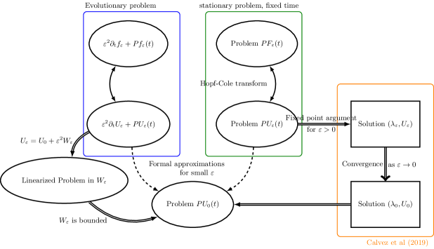
Figure 1. Scope of our paper compared to precedent work

The authors introduced an appropriate functional space controlling Lipschitz bound. They were then able to show the existence of $U_{\varepsilon}^{s}$ and its (local) uniqueness in that space. They also proved that $U_{\varepsilon}^{s}$ was converging when $\varepsilon\to 0$ towards solutions of equation $P_{t}U_{0}$, see Figure 1 for a schematic comparison of the scope of the present article article compared to previous work.

Here, to tackle the non stationary equation 1.3, we make the following assumptions of asymptotic growth on the selection function $m$, when $\left\lvert z\right\rvert\to\infty$.

Assumption 1.1.

We suppose that the function $m$ is a $\mathcal{C}^{5}(\mathbb{R})$ function, bounded below. We define the scalar function $\operatorname{z_{\ast}}$ as the following gradient flow:

(1.12) $$\operatorname{\dot{z}_{\ast}}(t)=-m^{\prime}(\operatorname{z_{\ast}}(t)),\quad t>0,$$

associated to an initial data $\operatorname{z_{\ast}}(0)$ prescribed. Next, we make the following assumptions :

• We suppose that $\operatorname{z_{\ast}}(0)$ lies next to a non-degenerate local minimum of $m$, $\operatorname{z_{\ast}^{s}}$ such that

  (1.13) $$\operatorname{z_{\ast}}(t)\xrightarrow[t\to\infty]{}\operatorname{z_{\ast}^{s}}.$$

• We also require that there exists a uniform positive lower bound on $M$ :

  (1.14) $$\inf_{(t,z)\in\mathbb{R}_{+}\times\mathbb{R}}M(t,z)>0.$$

• We make growth assumptions on $M$ in the following way:

  (1.15) $$\text{for }\,k=1,2,3,4,5:\quad(1+\left\lvert z-\operatorname{z_{\ast}}\right\rvert)^{\alpha}\dfrac{\partial_{z}^{k}M(t,z)}{M(t,z)}\in L^{\infty}(\mathbb{R}_{+}\times\mathbb{R})\,,$$

  for some $0<\alpha<1$, the same than in definition 1.3.

• We make a final assumption upon the behavior of $m$ at infinity, that is roughly that it has superlinear growth, uniformly in time:

  (1.16) $$\limsup_{z\to\infty}\left\lvert\frac{M(t,\overline{z})}{M(t,z)}\right\rvert:=a<\frac{1}{2},\quad\limsup_{z\to\infty}\left\lvert\frac{\partial_{z}M(t,\overline{z})}{\partial_{z}M(t,z)}\right\rvert<\infty.$$

The first assumption on $m$ and $\operatorname{z_{\ast}}$ guarantee the following local convexity property, at least for times $t$ large enough :

(1.17) $$\exists\,\mu_{0}>0,\ \exists t_{0}>0,\text{ such that~}\forall t\geqslant t_{0},\,m^{\prime\prime}(\operatorname{z_{\ast}}(t))\geqslant\mu_{0}.$$

Remark 1.2.

Based on the formulation of equation $P_{t}U_{0}$, the function $M$ must be positive. We require a uniform bound in equation 1.14 for technical reasons. It corresponds to a global assumption on the behavior of $\operatorname{z_{\ast}}$ and $m$, that further reduces the choice of $\operatorname{z_{\ast}}(0)$. This condition holds true for globally convex functions $m$. However we do not want to restrict our analysis to that case, so we suppose more generally that equation 1.14 is verified. A more detailed discussion on the behavior of the solution whether this condition is verified or not is carried out in section 9 with some numerical simulations displayed. Moreover, the decay assumptions equation 1.15 and equation 1.16 hold true if $m$ behaves like a polynomial function at least quadratic as $\left\lvert z\right\rvert\to+\infty$.

The purpose of this work is to rigorously prove the convergence of the solution of equation 1.3 towards a particular solution of equation $P_{t}U_{0}$. Given the general shape of $U_{0}$, see equation 1.11, it is natural to decompose $U_{\varepsilon}$ by separating the affine part from the rest:

(1.18) $$U_{\varepsilon}(t,z)=p_{\varepsilon}(t)+q_{\varepsilon}(t)(z-\operatorname{z_{\ast}}(t))+V_{\varepsilon}(t,z).$$

We require accordingly that at all times $t>0$,

$$V_{\varepsilon}(t,\operatorname{z_{\ast}})=\partial_{z}V_{\varepsilon}(t,\operatorname{z_{\ast}})=0,$$

which is another way of saying that the pair $(p_{\varepsilon},q_{\varepsilon})$ tune the affine part of $U_{\varepsilon}$. The pair $(q_{\varepsilon},V_{\varepsilon})$ is the main unknown of this problem. It is expected that $V_{\varepsilon}$ converges to $V^{\ast}$ when $\varepsilon\to 0$. Our analysis will be able to determine the limit of $q_{\varepsilon}$ even if it cannot be identified by the problem at $\varepsilon=0$. Indeed in equation $P_{t}U_{0}$, the linear part $q_{0}$ can be any constant. Our limit candidate for $q_{\varepsilon}$ is $q^{\ast}$, that we define as the solution of the following differential equation

(1.19) $$\dot{q}^{\ast}(t)=-m^{\prime\prime}(\operatorname{z_{\ast}}(t))q^{\ast}(t)+\frac{m^{(3)}(\operatorname{z_{\ast}}(t))}{2}-2m^{\prime\prime}(\operatorname{z_{\ast}}(t))m^{\prime}(\operatorname{z_{\ast}}(t)),$$

corresponding to an initial value of $q^{\ast}(0)$. Moreover we define $p^{\ast}$ as the function which verifies for a given $p^{\ast}(0)$,

(1.20) $$\dot{p}^{\ast}(t)=-m^{\prime}(\operatorname{z_{\ast}}(t))q^{\ast}(t)+m^{\prime\prime}(\operatorname{z_{\ast}}(t)).$$

Finally, the function

(1.21) $$U^{\ast}(t,z):=p^{\ast}(t)+q^{\ast}(t)(z-\operatorname{z_{\ast}}(t))+V^{\ast}(t,z)$$

will be our candidate for the limit of $U_{\varepsilon}$ when $\varepsilon\to 0$. The problem for $V_{\varepsilon}$ equivalent to equation 1.3, using equation 1.18, is:

(1.21) $$M(t,z)-\varepsilon^{2}\Big{(}\dot{p}_{\varepsilon}(t)+\dot{q}_{\varepsilon}(t)(z-\operatorname{z_{\ast}}(t))+m^{\prime}(\operatorname{z_{\ast}}(t))q_{\varepsilon}(t)\Big{)}-\varepsilon^{2}\partial_{t}V_{\varepsilon}(t,z)\\ =\mathcal{I}_{\varepsilon}(q_{\varepsilon},V_{\varepsilon})(t,z)\exp\Big{(}V_{\varepsilon}(t,z)-2V_{\varepsilon}\left(t,\bar{z}(t)\right)+V_{\varepsilon}(t,\operatorname{z_{\ast}}(t))\Big{)}.$$

One can notice that thanks to cancellations the functional $I_{\varepsilon}(U_{\varepsilon})$ does not depend on $p_{\varepsilon}$, which explains for the most part why we focus upon $(q_{\varepsilon},V_{\varepsilon})$. We choose to write $\mathcal{I}_{\varepsilon}(q_{\varepsilon},V_{\varepsilon})(t,z):=I_{\varepsilon}(U_{\varepsilon})(t,z)$ as a functional of both unknowns because we will study variations in both directions. One of the main difficulties to prove the link between equations 1.21 and $P_{t}U_{0}$ is that formally, the terms with the time derivatives in $q_{\varepsilon}$ and $V_{\varepsilon}$ vanish when $\varepsilon\to 0$. This makes our study belong to the class of singular limit problems.

Before stating our main result we need to define appropriate functional spaces. We first define a reference space $\mathcal{E}$, similar to the one introduced in Calvez et al., (2019) for the study of the stationary equation $PU_{\varepsilon}$ stat. However, compared to that case we will need more precise controls, which is why we introduce a subspace $\mathcal{F}$ with more stringent conditions.

Definition 1.3 (Functional spaces).

We define $\alpha<2-\frac{\ln 3}{\ln 2},$ such that $\alpha\in\left(0,1\right)$ and the corresponding functional space

$$\mathcal{E}=\Big{\{}v\in\mathcal{C}^{3}(\mathbb{R}_{+}\times\mathbb{R})\,|\,\forall t>0,\,v(t,\operatorname{z_{\ast}}(t))=\partial_{z}v(t,\operatorname{z_{\ast}}(t))=0\Big{\}}\\ \bigcap\left\{v\in\mathcal{C}^{3}(\mathbb{R}_{+}\times\mathbb{R})~\left|\begin{array}[]{rrr}\displaystyle\hfil&\left\lvert\partial_{z}v(t,z)\right\rvert\\ \displaystyle\hfil&\Big{(}1+\left\lvert z-\operatorname{z_{\ast}}(t)\right\rvert\Big{)}^{\alpha}\left\lvert\partial_{z}^{2}v(t,z)\right\rvert\\ \displaystyle\hfil&\Big{(}1+\left\lvert z-\operatorname{z_{\ast}}(t)\right\rvert\Big{)}^{\alpha}\left\lvert\partial_{z}^{3}v(t,z)\right\rvert\end{array}\right.\in L^{\infty}(\mathbb{R}_{+}\times\mathbb{R})\right\}$$

equipped with the norm

$$\left\lVert v\right\rVert_{\mathcal{E}}=\max\left(\sup_{(t,z)\in\mathbb{R}_{+}\times\mathbb{R}}\left\lvert\partial_{z}v(t,z)\right\rvert,\ \sup_{(t,z)\in\mathbb{R}_{+}\times\mathbb{R}}\Big{(}1+\left\lvert z-\operatorname{z_{\ast}}(t)\right\rvert\Big{)}^{\alpha}\left\lvert\partial_{z}^{2}v(t,z)\right\rvert\right.,\\ \left.\sup_{(t,z)\in\mathbb{R}_{+}\times\mathbb{R}}\Big{(}1+\left\lvert z-\operatorname{z_{\ast}}(t)\right\rvert\Big{)}^{\alpha}\left\lvert\partial_{z}^{3}v(t,z)\right\rvert\right).$$

We also define the subspace :

$$\mathcal{F}:=\mathcal{E}\cap\left\{v\in\mathcal{C}^{1}(\mathbb{R}_{+}\times\mathbb{R})~\left|\begin{array}[]{rrr}\displaystyle\hfil&\left\lvert 2v(t,\overline{z}(t))-v(t,z)\right\rvert\\ \displaystyle\hfil&\Big{(}1+\left\lvert z-\operatorname{z_{\ast}}(t)\right\rvert\Big{)}^{\alpha}\left\lvert\partial_{z}v(t,\overline{z}(t))-\partial_{z}v(t,z)\right\rvert\end{array}\right.\in L^{\infty}(\mathbb{R}_{+}\times\mathbb{R})\right\}$$

and we associate the corresponding norm :

$$\left\lVert v\right\rVert_{\mathcal{F}}=\max\left(\left\lVert v\right\rVert_{\mathcal{E}},\sup_{(t,z)\in\mathbb{R}_{+}\times\mathbb{R}}\left\lvert 2v(t,\overline{z}(t))-v(t,z)\right\rvert,\sup_{(t,z)\in\mathbb{R}_{+}\times\mathbb{R}}\Big{(}1+\left\lvert z-\operatorname{z_{\ast}}(t)\right\rvert\Big{)}^{\alpha}\left\lvert\partial_{z}v(t,\overline{z}(t))-\partial_{z}v(t,z)\right\rvert\right).$$

We will use the notational shortcut $\varphi_{\alpha}$ for the weight function :

$$\varphi_{\alpha}(t,z):=\Big{(}1+\left\lvert z-\operatorname{z_{\ast}}(t)\right\rvert\Big{)}^{\alpha}.$$

Since most of this paper is focused around the pair $(q_{\varepsilon},V_{\varepsilon})\in\mathbb{R}\times\mathcal{F}$, we will use the convenient notation $\left\lVert(q,V)\right\rVert:=\max\Big{(}\left\lvert q\right\rvert,\left\lVert V\right\rVert_{\mathcal{F}}\Big{)}$. Our main theorem is the following convergence result :

Theorem 1.4 (Convergence).

There exist $K_{0}$, $K^{\prime}_{0}$ and $\varepsilon_{0}>0$ such that if we make the following assumptions on the initial condition, for all $\varepsilon\leqslant\varepsilon_{0}$ :

$$\quad\left\lVert V_{\varepsilon}(0,\cdot)-V^{\ast}(0,\cdot)\right\rVert_{\mathcal{F}} \leqslant~\varepsilon^{2}K_{0},$$

$$\left\lvert q_{\varepsilon}(0)-q^{\ast}(0)\right\rvert \leqslant\varepsilon^{2}K_{0},\text{~and }$$

$$\quad\left\lvert p_{\varepsilon}(0)-p^{\ast}(0)\right\rvert \leqslant\varepsilon^{2}K_{0},$$

then we have uniform estimates of the solutions of the Cauchy problem:

$$\sup_{t>0}\ \left\lVert V_{\varepsilon}-V^{\ast}\right\rVert_{\mathcal{F}} \leqslant\varepsilon^{2}K^{\prime}_{0},$$

$$\sup_{t>0}\left\lvert q_{\varepsilon}(t)-q^{\ast}(t)\right\rvert \leqslant\varepsilon^{2}K^{\prime}_{0}$$

$$\sup_{t>0}\left\lvert p_{\varepsilon}(t)-p^{\ast}(t)\right\rvert \leqslant\varepsilon^{2}K^{\prime}_{0},$$

where $q^{\ast}$ is the solution of equation 1.19 associated to $q^{\ast}(0)$ and $p^{\ast}$ is the solution of equation 1.20 associated to $p^{\ast}(0)$. The function $V^{\ast}$ is defined in equation 1.10.

Therefore, as predicted, the limit of $U_{\varepsilon}$ when $\varepsilon\to 0$ is the function $p^{\ast}(t)+q^{\ast}(t)(z-\operatorname{z_{\ast}}(t))+V^{\ast}(t,z)$. Theorem 1.4 establish the stability, with respect to $\varepsilon$ and uniformly in time, of Gaussian distributions around the dynamics of the dominant trait driven by a gradient flow differential equation.

In Calvez et al., (2019) a fixed point argument was used to build solutions of the stationary problem when $\varepsilon\ll 1$. However, this method can no longer be applied in this case since the derivative in time breaks the structure that made the stationary problem equivalent to a fixed point mapping. In fact, in the present article, equation 1.5 and equation 1.3 are of different nature due to the fast time relaxation dynamics. This is one of the main difficulty of this work compared to Calvez et al., (2019). For this reason we replace the fixed point argument by a perturbative analysis. We introduce the following corrector terms, $\kappa_{\varepsilon},W_{\varepsilon}$, our aim is to bound them uniformly :

(1.22) $$V_{\varepsilon}(t,z) =V^{\ast}(t,z)+\varepsilon^{2}W_{\varepsilon}(t,z),$$

(1.23) $$q_{\varepsilon}(t) =q^{\ast}(t)+\varepsilon^{2}\kappa_{\varepsilon}(t).$$

The scalar $q^{\ast}$ , perturbed by $\varepsilon^{2}\kappa_{\varepsilon}$, will tune further the affine part of the solution. The function $W_{\varepsilon}$ measures the error made when approximating equation 1.3 by equation $P_{t}U_{0}$. We choose not to perturb $p_{\varepsilon}$ because we will see in section 5.2 that it can be straightforwardly deduced from the analysis.

This decomposition highlights a crucial part of our analysis, coming back to the initial equation $P_{t}f_{\varepsilon}$. Strikingly, the main contribution (in $\varepsilon$) to the solution is quadratic, see equation 1.2, and therefore it does not belong to the space of the corrective term $V_{\varepsilon}$. The order of precision is quite high since we are investigating the error made when approximating $f_{\varepsilon}$ by almost Gaussian distributions : $W_{\varepsilon}$ is of order $\varepsilon^{2}$, while $U_{\varepsilon}$ is of order $1$ in $\varepsilon$. The objective of this article is to show that $\kappa_{\varepsilon}$ and $W_{\varepsilon}$ are uniformly bounded with respect to time and $\varepsilon$.

2. Heuristics and method of proof

For this section only, we focus on the function $U_{\varepsilon}$ instead of $V_{\varepsilon}$ to get a heuristic argument in favor of the decomposition equation 1.18 and some elements supporting Theorem 1.4. We will denote $R_{\varepsilon}$ the perturbation such that we look for solutions of equation 1.3 under the following form:

$$U_{\varepsilon}(t,z)=U^{\ast}(t,z)+\varepsilon^{2}R_{\varepsilon}(t,z).$$

The function $U^{\ast}$, defined in equation 1.21 also solves equation $P_{t}U_{0}$. Plugging this perturbation into equation 1.3 yields the following perturbed equation for $R_{\varepsilon}$:

$$M(t,z)-\varepsilon^{2}\partial_{t}U^{\ast}(t,z)-\varepsilon^{4}\partial_{t}R_{\varepsilon}(t,z)=I_{\varepsilon}(U^{\ast}+\varepsilon^{2}R_{\varepsilon})(t,z)\times\\ \exp\Big{(}U^{\ast}(t,z)-2U^{\ast}\left(t,\bar{z}(t)\right)+U^{\ast}(t,\operatorname{z_{\ast}}(t))\Big{)}\exp\left(\varepsilon^{2}\Big{(}R_{\varepsilon}(t,z)-2R_{\varepsilon}\left(t,\bar{z}(t)\right)+R_{\varepsilon}(t,\operatorname{z_{\ast}}(t))\Big{)}\right).$$

By using equation $P_{t}U_{0}$, one gets that $R_{\varepsilon}$ solves the following :

$$M(t,z)-\varepsilon^{2}\partial_{t}U^{\ast}(t,z)-\varepsilon^{4}\partial_{t}R_{\varepsilon}(t,z)=\\ I_{\varepsilon}(U^{\ast}+\varepsilon^{2}R_{\varepsilon})(t,z)M(t,z)\exp\left(\varepsilon^{2}\Big{(}R_{\varepsilon}(t,z)-2R_{\varepsilon}\left(t,\bar{z}(t)\right)+R_{\varepsilon}(t,\operatorname{z_{\ast}}(t))\Big{)}\right).$$

To prove the boundedness of $R_{\varepsilon}$, solution to this nonlinear equation, we shall linearize it and show a stability result on the linearized problem (see Theorem 7.1). We explain here the heuristics about the linearization. We have already said that $I_{\varepsilon}$ is expected to converge to 1. Therefore by linearizing the exponential, a natural linearized equation appears to be :

(2.1) $$\varepsilon^{2}\partial_{t}\widetilde{R_{\varepsilon}}(t,z)=M(t,z)\Big{(}-\widetilde{R_{\varepsilon}}(t,z)+2\widetilde{R_{\varepsilon}}\left(t,\bar{z}(t)\right)-\widetilde{R_{\varepsilon}}(t,\operatorname{z_{\ast}}(t))\Big{)},$$

For clarity we denote by $T$ the linear operator:

$$T(R)(t,z):=M(t,z)\Big{(}2R(t,\overline{z}(t))-R(t,z)+R(t,\operatorname{z_{\ast}}(t))\Big{)}.$$

We know precisely what are the eigen-elements of this linear operator. The eigenvalue $0$ has multiplicity two, the eigenspace consisting of affine functions. More generally one can get every eigenvalue by differentiating iteratively the operator and evaluating at $z=\operatorname{z_{\ast}}$. This corresponds to the following table:

Eigenvalue :	$0$	$0$	$-\frac{1}{2}$	$-\frac{3}{4}$	…
Dual eigenvector :	$\delta_{\operatorname{z_{\ast}}(t)}$	$\delta^{\prime}_{\operatorname{z_{\ast}}(t)}$	$\delta^{\prime\prime}_{\operatorname{z_{\ast}}(t)}$	$\delta^{(3)}_{\operatorname{z_{\ast}}(t)}$	…

Table 1. Eigen-elements of $T$.

This explains why $R_{\varepsilon}$ should be decomposed between affine parts and the rest, and as a consequence, also the solution $U_{\varepsilon}$ we are investigating. The scalars $p_{\varepsilon}$ and $q_{\varepsilon}$ of the decomposition equation 1.18 correspond to the projection of $U_{\varepsilon}$ upon the eigenspace associated to the (double) eigenvalue $0$. On the other hand the rest is expected to remain uniformly bounded since the corresponding eigenvalues are negative, below $-\frac{1}{2}$.

Beyond the heuristics about the stability, this linear analysis also illustrates the discrepancy between $V_{\varepsilon}$ and $q_{\varepsilon}$ in Theorem 1.4. While $V_{\varepsilon}$ is expected to relax to a n explicit bounded value arbitrary quickly as $\varepsilon\to 0$ (fast dynamics), this is not true for $q^{\ast}$ which solves a differential equation (slow dynamics):

$$\dot{q}^{\ast}(t)=-m^{\prime\prime}(\operatorname{z_{\ast}}(t))q^{\ast}(t)+\frac{m^{(3)}(\operatorname{z_{\ast}}(t))}{2}-2m^{\prime\prime}(\operatorname{z_{\ast}}(t))m^{\prime}(\operatorname{z_{\ast}}(t)).$$

We can infer that the second eigenvalue $0$ in Table 1 is in fact inherited from $-\varepsilon^{2}m^{\prime\prime}(\operatorname{z_{\ast}}(t))$ at $\varepsilon>0$, which explains that we can read $q^{\ast}$ at this order.

The technique we will use in the following sections to bound $W_{\varepsilon}$ in $\mathcal{F}$ will seem more natural in the light of this formal analysis. The first step will be to work around $\operatorname{z_{\ast}}$, the base point of the dual eigen-elements in Table 1. We will derive uniform bounds up to the third derivative to estimate $W_{\varepsilon}$, see Theorem 7.1.

By plugging the expansions of equation 1.22 and equation 1.23 associated to the decomposition equation 1.18 and the logarithmic transform equation 1.2 into our original model equation $P_{t}f_{\varepsilon}$, we obtain the following main reference equation that we will study in the rest of this article :

(2.2) $$M(t,z)-\varepsilon^{2}\Big{(}\dot{p}_{\varepsilon}(t)+\dot{q}^{\ast}(t)(z-\operatorname{z_{\ast}})+m^{\prime}(\operatorname{z_{\ast}})q^{\ast}(t)+\partial_{t}V^{\ast}(t,z)\Big{)}\\ -\varepsilon^{4}\Big{(}\dot{\kappa}_{\varepsilon}(t)(z-\operatorname{z_{\ast}})+m^{\prime}(\operatorname{z_{\ast}})\kappa_{\varepsilon}(t)+\partial_{t}W_{\varepsilon}(t,z)\Big{)}=M(t,z)\mathcal{I}_{\varepsilon}(q^{\ast}+\varepsilon^{2}\kappa_{\varepsilon},V^{\ast}+\varepsilon^{2}W_{\varepsilon})\times\\ \exp\left(\varepsilon^{2}\Big{(}W_{\varepsilon}(t,z)-2W_{\varepsilon}\left(t,\bar{z}(t)\right)+W_{\varepsilon}(\operatorname{z_{\ast}}(t))\Big{)}\right).$$

Our main objective will be to linearize equation 2.2, in order to deduce the boundedness of the unknowns, $(\kappa_{\varepsilon}\,W_{\varepsilon})$, by working on the linear part of the equations. We will need to investigate different scales (in $\varepsilon$) to capture the different behaviors of each contribution.

We will pay attention to the remaining terms. We will use the classical notation $O(1)$ and $O(\varepsilon)$, and we will write $\left\lVert(\kappa_{\varepsilon},W_{\varepsilon})\right\rVert O(\varepsilon)$ to illustrate when the constants of $O(\varepsilon)$ depend on $(\kappa_{\varepsilon},W_{\varepsilon})$. We also define a refinement of the classical notation $O(\varepsilon)$ :

Definition 2.1 ($O^{\ast}(\varepsilon^{\alpha})$).

For $\alpha\in\mathbb{N}$, we say that a function $g(\varepsilon,t,z)$ is such that $g(\varepsilon,t,z)=O^{\ast}(\varepsilon^{\alpha})$ if there exists $\varepsilon^{\ast}$ such that for all $\varepsilon~\leqslant\varepsilon^{\ast}$ it verifies :

$$\left\lvert g(\varepsilon,t,z)\right\rvert\leqslant C^{\ast}\varepsilon^{\alpha},$$

and the constants $\varepsilon^{\ast},C^{\ast}$ depend only on the pair $(q^{\ast},V^{\ast})$.

More generally, when we write $O(\varepsilon)$, the constants involved may a priori depend upon the pair $(\kappa_{\varepsilon},W_{\varepsilon})$. Our intent is to make the dependency of the constants clear when we linearize. This will prove to be a crucial point when we will go back to the non-linear problem equation 2.2. We will see that all the terms that do not have a sufficient order in $\varepsilon$ to be negligible will be $O^{\ast}(1)$, and therefore uniformly bounded independently of $(\kappa_{\varepsilon},W_{\varepsilon})$. A key point of our analysis is to segregate those terms when doing the linearization.

The rest of the paper is organized as follows :

• First we prove some properties upon the reference pair $(q^{\ast},V^{\ast})$ around which all the terms of equation 2.2 are linearized.

• A key part of our perturbative analysis is to be able to linearize $\mathcal{I}_{\varepsilon}$, which we do in section 4 thanks to cautious estimates upon the directional derivatives.

• We derive an equation on $\kappa_{\varepsilon}$ in section 5.1, and later a linear approximated equation for $W_{\varepsilon}$, and more importantly for all of its derivatives in section 6, while controlling precisely the error terms.

• We show the boundedness of the solutions of the linear problem in the space $\mathcal{F}$, see section 7, mainly through maximum principles and a dyadic division of the space to take into account the non local behavior of the infinitesimal operator. This is the content of Theorem 7.1.

• Finally, we tackle the proof of Theorem 1.4 in the section 8.

• To conclude, in section 9 we discuss some of our assumptions made in Assumption 1.1, illustrated by some numerical simulations.

Index of Notations

$U_{\varepsilon}$	Perturbation of Gaussian distribution to solve the Cauchy problem equation $P_{t}f_{\varepsilon}$, see equation 1.2
$m$	Selection function
$I_{\varepsilon}$	Residual shape of the infinitesimal operator after transformation, defined in equation 1.4
$\operatorname{z_{\ast}}$	Dominant trait in the population, solves a gradient flow ODE: equation 1.12
$\bar{z}$	$\frac{z+\operatorname{z_{\ast}}}{2}$
$M$	$1+m(z)-m(\operatorname{z_{\ast}}(t))-m^{\prime}(\operatorname{z_{\ast}}(t))(z-\operatorname{z_{\ast}}(t))$
$p_{\varepsilon},q_{\varepsilon},V_{\varepsilon}$	$U_{\varepsilon}(t,z)=p_{\varepsilon}(t)+q_{\varepsilon}(t)(z-\operatorname{z_{\ast}}(t))+V_{\varepsilon}(t,z)$
$\mathcal{I}_{\varepsilon}$	Same thing as $I_{\varepsilon}$ but as a function of two variables : $\mathcal{I}_{\varepsilon}(q_{\varepsilon},V_{\varepsilon})=I_{\varepsilon}(U_{\varepsilon})$
$U^{\ast}$	Limit of $U_{\varepsilon}$ when $\varepsilon\to 0$
$p^{\ast},q^{\ast},V^{\ast}$	$U^{\ast}(t,z)=p^{\ast}(t)+q^{\ast}(t)(z-\operatorname{z_{\ast}}(t))+V^{\ast}(t,z)$
$(\kappa_{\varepsilon},W_{\varepsilon})$	$q_{\varepsilon}=\kappa_{\varepsilon}+\varepsilon^{2}\kappa_{\varepsilon},V_{\varepsilon}=V^{\ast}+\varepsilon^{2}W_{\varepsilon}$
$\Xi_{\varepsilon}(t,z)$	$W_{\varepsilon}(t,z)-2W_{\varepsilon}(t,\overline{z})$
$\mathcal{E}$	Functional space to measure $V_{\varepsilon}$
$\varphi_{\alpha}$	Weight function, $\varphi_{\alpha}(t,z)=\Big{(}1+\left\lvert z-\operatorname{z_{\ast}}(t)\right\rvert\Big{)}^{\alpha}$
$\mathcal{F}$	Functional space to measure $W_{\varepsilon}$
$\left\lVert(g,W)\right\rVert$	$\max\Big{(}\left\lvert g\right\rvert,\left\lVert W\right\rVert_{\mathcal{F}}\Big{)}$, or $\max\Big{(}\left\lvert g\right\rvert,\left\lVert W\right\rVert_{\mathcal{E}}\Big{)}$ depending on the context
$\mathcal{E}^{\ast}$	Functional space to measure $V^{\ast}$
$K^{\ast}$	Uniform bound of $V^{\ast}$ in $\mathcal{E}^{\ast}$
$O^{\ast}(\varepsilon)$	Special negligible term $O(\varepsilon)$ where the constants depend only on $K^{\ast}$
$\mathcal{I}_{\varepsilon}^{\ast}$	$\mathcal{I}_{\varepsilon}(q^{\ast},V^{\ast})$
$Q(y_{1},y_{2})$	$\frac{1}{2}y_{1}y_{2}+\frac{3}{4}(y_{1}^{2}+y_{2}^{2})$
$Y$	$(y_{1},y_{2})$
$\mathcal{D}_{\varepsilon}(V)(Y,t,z)$	$V(t,\overline{z})-\frac{1}{2}V(t,\overline{z}+\varepsilon y_{1})-\frac{1}{2}V(t,\overline{z}+\varepsilon y_{2})$
$\mathcal{D}_{\varepsilon}^{\ast}(V)(y,t)$	$V(t,\operatorname{z_{\ast}})-V(t,\operatorname{z_{\ast}}+\varepsilon y)$
$\left\lVert W\right\rVert_{\infty}$	$\displaystyle\sup_{(t,z)\in\mathbb{R}_{+}\times\mathbb{R}}\left\lvert W(t,z)\right\rvert$
$dG_{\varepsilon}^{\ast},dN_{\varepsilon}^{\ast}$	Probability densities that simplify some notations in section 4.3, defined in equation 4.26 and equation 4.27.
$O^{\ast}_{0}(1)$	$\max\Big{(}O^{\ast}(1),O^{\ast}(1)\left\lVert W_{\varepsilon}(0,\cdot)\right\rVert_{\mathcal{F}}\Big{)}$ (where we slightly abuse notation)
$B_{0}$	Ball that contains $\operatorname{z_{\ast}}$, see figure 2
$D_{n}$	The nth dyadic ring defined in equation 7.2, see figure 2
$\left\lVert W\right\rVert_{\infty}^{0}$,   $\left\lVert W\right\rVert_{\infty}^{n}$	$\displaystyle\sup_{(t,z)\in\mathbb{R}_{+}\times B_{0}}\left\lvert W(t,z)\right\rvert$ ,  $\displaystyle\sup_{(t,z)\in\mathbb{R}_{+}\times D_{n}}\left\lvert W(t,z)\right\rvert$

3. Preliminary results : estimates of $\mathcal{I}_{\varepsilon}^{\ast}$ and $V^{\ast}$

3.1. Control of $(q^{\ast},V^{\ast})$

Before tackling the main difficulties of this article, we first state some controls on the function $V^{\ast}$, solution of equation $P_{t}U_{0}$. Most of them use the explicit expression of equation 1.10 and were proved in Calvez et al., (2019). To be able to measure this function we introduce another functional space, with more constraints.

Definition 3.1 (Subspace $\mathcal{E}^{\ast}$).

We define $\mathcal{E}^{\ast}$ as the following subspace of $\mathcal{E}$ :

$$\mathcal{E}^{\ast}:=\mathcal{E}\cap\left\{v\in\mathcal{C}^{5}(\mathbb{R}_{+}\times\mathbb{R})~\left|\begin{array}[]{rrr}\displaystyle\hfil&\varphi_{\alpha}(t,z)\left\lvert\partial_{z}^{4}v(t,z)\right\rvert\\ \displaystyle\hfil&\varphi_{\alpha}(t,z)\left\lvert\partial_{z}^{5}v(t,z)\right\rvert\end{array}\right.\in L^{\infty}(\mathbb{R}_{+}\times\mathbb{R})\right\}$$

We equip it with the norm $\left\lVert\cdot\right\rVert_{\ast}$ :

$$\left\lVert v\right\rVert_{\ast}=\max\left(\left\lVert v\right\rVert_{\mathcal{E}},\sup_{(t,z)\in\mathbb{R}_{+}\times\mathbb{R}}\varphi_{\alpha}(t,z)\left\lvert\partial_{z}^{4}v(t,z)\right\rvert,\sup_{(t,z)\in\mathbb{R}_{+}\times\mathbb{R}}\varphi_{\alpha}(t,z)\left\lvert\partial_{z}^{5}v(t,z)\right\rvert\right).$$

Our intention with the successive definitions of the functional spaces is to be able to measure each term of the decomposition made in equation 1.22 as follows:

$$\underbrace{V_{\varepsilon}}_{\mathcal{E}}=\underbrace{V^{\ast}}_{\mathcal{E}^{\ast}}+\varepsilon^{2}\underbrace{W_{\varepsilon}}_{\mathcal{F}}.$$

The fact that $V^{\ast}\in\mathcal{E}^{\ast}$ is part of the claim of the following lemma.

Lemma 3.2 (Properties of $V^{\ast}$).

The function $V^{\ast}$ belongs to the space $\mathcal{E}^{\ast}$. Moreover,

(3.1) $$\partial_{z}^{2}V^{\ast}(t,\operatorname{z_{\ast}})=2m^{\prime\prime}(\operatorname{z_{\ast}}),\quad\quad\partial_{z}^{3}V^{\ast}(t,\operatorname{z_{\ast}})=\frac{4}{3}m^{(3)}(\operatorname{z_{\ast}}).$$

Proof.

Precise estimates of the summation operator that defines $V^{\ast}$ in equation 1.10 are studied in Calvez et al., (2019). They can be applied there thanks to the decay assumptions about $M$, equation 1.15. The only difference here is that an uniform bound for the fourth and fifth derivative are required. The proofs of those bounds rely solely upon the assumption made in equation 1.15, for the fourth and fifth derivative of $M$. This shows that $V^{\ast}\in\mathcal{E}^{\ast}$. Explicit computations based on the formula equation 1.10 prove the relationships equation 3.1. ∎

A consequence of Lemma 3.2 is that since $m^{\prime\prime}(\operatorname{z_{\ast}}(t))>0$ for $t>t_{0}$, thanks to equation 1.17, which implies that $V^{\ast}$ is locally convex around $\operatorname{z_{\ast}}(t)$. However we need more information upon $V^{\ast}$ than the space it belongs to. We will bound $(q^{\ast},V^{\ast})$ independently of time. This is the content of the following result:

Proposition 3.3 (Uniform bound on $(q^{\ast},V^{\ast})$).

There exists a constant $K^{\ast}$ such that for $j=0,1,2$ and $3$, we have

$$\max~\Big{(}\left\lVert V^{\ast}\right\rVert_{\ast},\left\lVert q^{\ast}\right\rVert_{L^{\infty}(\mathbb{R}_{+})},\left\lVert\partial_{t}\,\partial_{z}^{j}V^{\ast}\right\rVert_{L^{\infty}(\mathbb{R}_{+}\times\mathbb{R})}\Big{)} \leqslant K^{\ast}.$$

Proof of Proposition 3.3.

For the estimates upon $V^{\ast}$ and $\partial_{t}V^{\ast}$, it is a direct consequence of the definition of $\mathcal{E}^{\ast}$ and the explicit formula equation 1.10. The technique to bound the sums is to distinguish between the small and large indices, it was detailed in Calvez et al., (2019).

For $q^{\ast}$, one must look to equation 1.19. The boundedness of $q^{\ast}$ is a straightforward consequence of the convexity of $m$ at $\operatorname{z_{\ast}}(t)$ for large times, see equation 1.17 and the convergence of $\operatorname{z_{\ast}}$ to bound the other terms.∎

3.2. Estimates of $\mathcal{I}_{\varepsilon}^{\ast}$ and its derivatives

We next define a notational shortcut for the functional $\mathcal{I}_{\varepsilon}$ introduced in equation 1.4, when it is evaluated at the reference pair $(q^{\ast},V^{\ast})$:

$$\mathcal{I}_{\varepsilon}^{\ast}:=\mathcal{I}_{\varepsilon}(q^{\ast},V^{\ast}).$$

This section is devoted to get precise estimates of this function. This will be crucial for the linearization of $\mathcal{I}_{\varepsilon}(q^{\ast}+\varepsilon^{2}\kappa_{\varepsilon},V^{\ast}+\varepsilon^{2}W_{\varepsilon})$ as can be seen on the full equation 2.2.

Proposition 3.4 (Estimation of $\mathcal{I}_{\varepsilon}^{\ast}$).

$$\mathcal{I}_{\varepsilon}^{\ast}(t,z)=1+O^{\ast}(\varepsilon^{2}),$$

where the constants of $O^{\ast}(\varepsilon^{2})$ depend only on $K^{\ast}$, introduced in Proposition 3.3, as defined by definition 2.1.

The proof consists in exact Taylor expansion in $\varepsilon$. Very similar expansions were performed in (Calvez et al.,, 2019, Lemma 3.1), we adapt the method of proof here, since it will be used extensively throughout this article.

Proof of Proposition 3.4.

We recall that by Proposition 3.3, $\max(\left\lvert q^{\ast}\right\rvert,\left\lVert V^{\ast}\right\rVert_{\ast})\leqslant K^{\ast}$ , and, by definition

$$\mathcal{I}_{\varepsilon}^{\ast}(t,z)=~\\ \frac{\displaystyle\iint_{\mathbb{R}^{2}}e^{-Q(y_{1},y_{2})}\exp\Big{(}-\varepsilon q^{\ast}(t)(y_{1}+y_{2})+2V^{\ast}(t,\overline{z})-V^{\ast}(t,\overline{z}+\varepsilon y_{1})-V^{\ast}(t,\overline{z}+\varepsilon y_{2})\Big{)}dy_{1}dy_{2}}{\displaystyle\sqrt{\pi}\int_{\mathbb{R}}e^{-\frac{1}{2}\left\lvert y\right\rvert^{2}}\exp\Big{(}-\varepsilon q^{\ast}(t)y+V^{\ast}(t,\operatorname{z_{\ast}})-V^{\ast}(t,\operatorname{z_{\ast}}+\varepsilon y)\Big{)}dy}\\ :=\frac{N(t,z)}{D(t)},$$

where $Q$ the quadratic form appearing after the rescaling of the infinitesimal operator in equation 1.4:

$$Q(y_{1},y_{2}):=\frac{1}{2}y_{1}y_{2}+\frac{3}{4}(y_{1}^{2}+y_{2}^{2}).$$

This quadratic form will appear very frequently in what follows, mostly, as here, through the bi-variate Gaussian distribution it defines. Once and for all we state that a correct normalization of this Gaussian distribution is:

$$\frac{1}{\sqrt{2}\pi}\iint_{\mathbb{R}^{2}}e^{-Q(y_{1},y_{2})}dy_{1}dy_{2}=1.$$

We start the estimates with the more complicated term, the numerator $N$. With an exact Taylor expansion inside the exponential, there exists generic $0<\xi_{i}<1$, for $j=1,2$, such that

$$N(t,z)=\displaystyle\dfrac{1}{\sqrt{2}\pi}\iint_{\mathbb{R}^{2}}e^{-Q(y_{1},y_{2})}\exp\Big{[}-\varepsilon q^{\ast}(t)(y_{1}+y_{2})-\varepsilon(y_{1}+y_{2})\partial_{z}V^{\ast}(t,\overline{z})\\ -\frac{\varepsilon^{2}}{2}\Big{(}y_{1}^{2}\partial_{z}^{2}V^{\ast}(t,\overline{z}+\varepsilon\xi_{1}y_{1})+y_{2}^{2}\partial_{z}^{2}V^{\ast}(t,\overline{z}+\varepsilon\xi_{2}y_{2})\Big{)}\Big{]}dy_{1}dy_{2}$$

Moreover we can write for some $\theta=\theta(y_{1},y_{2})\in(0,1)$,

$$\exp(-\varepsilon P)=1-\varepsilon P+\frac{\varepsilon^{2}P^{2}}{2}\exp(-\theta\varepsilon P)\,,$$

$$P=(y_{1}+y_{2})\Big{(}q^{\ast}(t)+\partial_{z}V^{\ast}(t,\overline{z})\Big{)}+\dfrac{\varepsilon}{2}\Big{(}y_{1}^{2}\partial_{z}^{2}V^{\ast}(t,\overline{z}+\varepsilon\xi_{1}y_{1})+y_{2}^{2}\partial_{z}^{2}V^{\ast}(t,\overline{z}+\varepsilon\xi_{2}y_{2})\Big{)}.$$

such that

(3.2) $$\quad|P|\leqslant K^{\ast}\left(\left\lvert y_{1}\right\rvert+\left\lvert y_{2}\right\rvert+\frac{\varepsilon(y_{1}^{2}+y_{2}^{2})}{2}\right),$$

Combining the expansions, we find:

$$N(t,z) =\frac{1}{\sqrt{2}\pi}\iint_{\mathbb{R}^{2}}e^{-Q(y_{1},y_{2})}\Big{(}1-\varepsilon P+\frac{\varepsilon^{2}P^{2}}{2}\exp(-\theta\varepsilon P)\Big{)}dy_{1}dy_{2},$$

(3.3) $$=1-\varepsilon\frac{1}{\sqrt{2}\pi}\iint_{\mathbb{R}^{2}}e^{-Q(y_{1},y_{2})}Pdy_{1}dy_{2}+\frac{\varepsilon^{2}}{2\sqrt{2}\pi}\iint_{\mathbb{R}^{2}}e^{-Q(y_{1},y_{2})}P^{2}\exp(-\theta\varepsilon P)dy_{1}dy_{2}$$

The key part is the cancellation of the terms $O(\varepsilon)$ due to the symmetry of $Q$ :

$$\frac{1}{\sqrt{2}\pi}\iint_{\mathbb{R}^{2}}e^{-Q(y_{1},y_{2})}(y_{1}+y_{2})dy_{1}dy_{2}=0.$$

Therefore :

$$\frac{\varepsilon}{\sqrt{2}\pi}\iint_{\mathbb{R}^{2}}e^{-Q(y_{1},y_{2})}Pdy_{1}dy_{2}=\frac{\varepsilon^{2}}{2\sqrt{2}\pi}\iint_{\mathbb{R}^{2}}e^{-Q(y_{1},y_{2})}\Big{(}y_{1}^{2}\partial_{z}^{2}V^{\ast}(t,\overline{z}+\varepsilon\xi_{1}y_{1})+y_{2}^{2}\partial_{z}^{2}V^{\ast}(t,\overline{z})+\varepsilon\xi_{2}y_{2})\Big{)}dy_{1}dy_{2}.$$

And we get the estimate

$$\left\lvert\frac{\varepsilon}{\sqrt{\pi}}\iint_{\mathbb{R}^{2}}e^{-Q(y_{1},y_{2})}Pdy_{1}dy_{2}\right\rvert \leqslant\frac{\varepsilon^{2}}{2\sqrt{2}\pi}\iint_{\mathbb{R}^{2}}e^{-Q(y_{1},y_{2})}\Big{(}y_{1}^{2}+y_{2}^{2}\Big{)}K^{\ast}dy_{1}dy_{2}$$

$$\leqslant O^{\ast}(\varepsilon^{2}).$$

Thanks to equation 3.2 it is easy to verify that the last term of equation 3.3 behaves similarly:

$$\frac{\varepsilon^{2}}{2\sqrt{2}\pi}\iint_{\mathbb{R}^{2}}e^{-Q(y_{1},y_{2})}P^{2}\exp(-\theta\varepsilon P)dy_{1}dy_{2}=O^{\ast}(\varepsilon^{2}).$$

Indeed, it states that the term $P$ is at most quadratic with respect to $y_{i}$ so $Q+\theta\varepsilon P$ is uniformly bounded below by a positive quadratic form for $\varepsilon$ small enough. This shows that

$$N(t,z)=1+O^{\ast}(\varepsilon^{2}).$$

The denominator is easier, with the same arguments, using the Gaussian density :

$$D(t)=1+O^{\ast}(\varepsilon^{2}).$$

Combining the estimates of $N$ and $D$, we get the desired result. ∎

There exists a link between $q^{\ast}$ and $\partial_{z}\mathcal{I}_{\varepsilon}^{\ast}(t,\operatorname{z_{\ast}})$, which is in fact the motivation behind the choice of $q^{\ast}$.

Proposition 3.5 (Link between $q^{\ast}$ and $\partial_{z}\mathcal{I}_{\varepsilon}^{\ast}(t,\operatorname{z_{\ast}})$).

$$\partial_{z}\mathcal{I}_{\varepsilon}^{\ast}(t,\operatorname{z_{\ast}}(t))=\varepsilon^{2}\left(m^{\prime\prime}(\operatorname{z_{\ast}}(t))q^{\ast}(t)-\frac{m^{(3)}(\operatorname{z_{\ast}}(t))}{2}\right)+O^{\ast}(\varepsilon^{4}),$$

where the constants of $O^{\ast}(\varepsilon^{4})$ only depend on $K^{\ast}$.

The proof of this result was the content of (Calvez et al.,, 2019, Lemma 3.1) and only requires that $(q^{\ast},V^{\ast})$ is uniformly bounded, as stated in Proposition 3.3. Its proof follows the same procedure of exact Taylor expansions as in the one of Proposition 3.4.

It will be useful to dispose of estimates of $\partial_{z}\mathcal{I}_{\varepsilon}^{\ast}$ not only at the point $\operatorname{z_{\ast}}$. They are less precise, as stated in the following proposition:

Proposition 3.6 (Estimates of the decay of the derivatives of $\mathcal{I}_{\varepsilon}^{\ast}$).

There exists a constant $\varepsilon_{\ast}$ that depends only on $K^{\ast}$ such that for all $\varepsilon\leqslant\varepsilon\ast$, for $j=1,2,3$:

$$\sup_{(t,z)\in\mathbb{R}_{+}\times\mathbb{R}}\varphi_{\alpha}(t,z)\left\lvert\partial_{z}^{(j)}\mathcal{I}_{\varepsilon}^{\ast}(t,z)\right\rvert=O^{\ast}(\varepsilon^{2}).$$

To shortcut notations, we introduce the following difference operator that appears in the integral $\mathcal{I}_{\varepsilon}$ see equation 1.4 :

(3.4) $$\mathcal{D}_{\varepsilon}(V)(Y,t,z) :=V(t,\overline{z})-\frac{1}{2}V(t,\overline{z}+\varepsilon y_{1})-\frac{1}{2}V(t,\overline{z}+\varepsilon y_{2}),\quad Y=(y_{1},y_{2}),$$

(3.5) $$\mathcal{D}_{\varepsilon}^{\ast}(V)(y,t) :=V(t,\operatorname{z_{\ast}})-V(t,\operatorname{z_{\ast}}+\varepsilon y).$$

We will use the following technical lemma giving an estimate of the weight function against the derivatives of a given function.

Lemma 3.7 (Influence of the weight function.).

There exists a constant $C$ such that for each ball $B$ of $\mathcal{E}^{\ast}$ or $\mathcal{F}$, there exists $\varepsilon_{B}$ such that for every $W\in B$, for every $y\in\mathbb{R}$ and $\varepsilon\leqslant\varepsilon_{B}$, for $j=2,3,4$ or $5$:

$$\varphi_{\alpha}(t,z)\left\lvert\partial_{z}^{(j)}W(t,\overline{z}(t)+\varepsilon y)\right\rvert \leqslant C\left\lVert W\right\rVert \text{ if}~\left\lvert y\right\rvert\leqslant\left\lvert z-\operatorname{z_{\ast}}(t)\right\rvert,$$

$$\leqslant(1+\left\lvert y\right\rvert^{\alpha})\left\lVert W\right\rVert.$$ otherwise,

with $\left\lVert W\right\rVert=\left\lVert W\right\rVert_{\ast}$ or $\left\lVert W\right\rVert_{\mathcal{F}}$ depending on the case.

The Proposition 3.6 is a prototypical result. It will be followed by a series of similar statements. Therefore, we propose two different proofs. In the first one, we write exact Taylor expansions. However the formalism is heavy, which is why we propose next a formal argument, where the Taylor expansions are written without exact rests for the sake of clarity.

In the rest of this paper more complicated estimates will be proved, in the spirit of Proposition 3.6, see Propositions 4.1 and 4.8 for instance. The notations and formulas will be very long, so we shall only write the ”formal” parts of the argument. However it can all be made rigorous, as below.

Proof of Proposition 3.6.

First, write the expression for the derivative, using our notation $\mathcal{D}_{\varepsilon}$ introduced in equation 3.4 :

(3.6) $$\partial_{z}\mathcal{I}_{\varepsilon}^{\ast}(t,z) =\frac{\displaystyle\iint_{\mathbb{R}^{2}}e^{-Q(y_{1},y_{2})}\exp\Big{(}-\varepsilon q^{\ast}(y_{1}+y_{2})+2\mathcal{D}_{\varepsilon}(V^{\ast})(Y,t,z)\Big{)}\mathcal{D}_{\varepsilon}(\partial_{z}V^{\ast})(Y,t,z)dy_{1}dy_{2}}{\displaystyle\sqrt{\pi}\int_{\mathbb{R}}e^{-\frac{1}{2}\left\lvert y\right\rvert^{2}}\exp\Big{(}-\varepsilon q^{\ast}y+\mathcal{D}_{\varepsilon}^{\ast}(V^{\ast})(y,t)\Big{)}dy},$$

$$:=\frac{N(t,z)}{D(t)}.$$

We only focus on the numerator. The denominator $D$ can be handled similarly as in the proof of Proposition 3.4, where we show that it is essentially $1+O^{\ast}(\varepsilon^{2})$. We perform two Taylor expansions in the numerator $N$, namely:

(3.7) $$\begin{cases}2\mathcal{D}_{\varepsilon}(V^{\ast})(Y,t,\overline{z})=-\varepsilon(y_{1}+y_{2})\partial_{z}V^{\ast}(t,\overline{z})-\dfrac{\varepsilon^{2}}{2}\Big{(}y_{1}^{2}\partial_{z}^{2}V^{\ast}(t,\overline{z}+\varepsilon\xi_{1}y_{1})+y_{2}^{2}\partial_{z}^{2}V^{\ast}(t,\overline{z}+\varepsilon\xi_{2}y_{2})\Big{)},\vskip 6.0pt plus 2.0pt minus 2.0pt\\ \displaystyle\mathcal{D}_{\varepsilon}(\partial_{z}V^{\ast})(Y,t,\overline{z})=-\dfrac{\varepsilon(y_{1}+y_{2})}{2}\partial_{z}^{2}V^{\ast}(t,\overline{z})-\dfrac{\varepsilon^{2}}{4}\Big{(}y_{1}^{2}\partial_{z}^{3}V^{\ast}(t,\overline{z}+\varepsilon\xi_{1}y_{1})+y_{2}^{2}\partial_{z}^{3}V^{\ast}(t,\overline{z}+\varepsilon\xi_{2}y_{2})\Big{)},\end{cases}$$

where $\xi_{i}$ denote some generic number such that $0<\xi<1$ for $i=1,2$. Moreover, we can write

(3.8) $$\exp(-\varepsilon P)=1-\varepsilon P\exp(-\theta\varepsilon P)\,\quad\text{~with }\\ P:=(y_{1}+y_{2})\Big{(}\partial_{z}V^{\ast}(t,\overline{z})+q^{\ast}\Big{)}+\dfrac{1}{2}\Big{(}y_{1}^{2}\partial_{z}^{2}V^{\ast}(t,\overline{z}+\varepsilon\xi_{1}y_{1})+y_{2}^{2}\partial_{z}^{2}V^{\ast}(t,\overline{z}+\varepsilon\xi_{2}y_{2})\Big{)}\,$$

for some $\theta=\theta(y_{1},y_{2})\in(0,1)$. Combining the expansions, we find:

$$\varphi_{\alpha}(t,z)\partial_{z}\mathcal{I}_{\varepsilon}^{\ast}(t,z)=\dfrac{\varphi_{\alpha}(t,z)}{\sqrt{2}\pi}\displaystyle\iint_{\mathbb{R}^{2}}e^{-Q(y_{1},y_{2})}\left(1-\varepsilon P\exp(-\theta\varepsilon P)\right)\\ \times\left(-\dfrac{\varepsilon(y_{1}+y_{2})}{2}\partial_{z}^{2}V^{\ast}(t,\overline{z})-\dfrac{\varepsilon^{2}}{4}\Big{(}y_{1}^{2}\partial_{z}^{3}V^{\ast}(t,\overline{z}+\varepsilon\xi_{1}y_{1})+y_{2}^{2}\partial_{z}^{3}V^{\ast}(t,\overline{z}+\varepsilon\xi_{2}y_{2})\Big{)}\right)dy_{1}dy_{2}\,.$$

The crucial point is the cancellation of the $O(\varepsilon)$ contribution due to the symmetry of $Q$, as already observed above:

$$\iint_{\mathbb{R}^{2}}e^{-Q(y_{1},y_{2})}(y_{1}+y_{2})dy_{1}dy_{2}=0\,.$$

So, it remains

$$\varphi_{\alpha}(t,z)N(t,z)=\\ -\varepsilon^{2}\dfrac{\varphi_{\alpha}(t,z)}{4\sqrt{2}\pi}\iint_{\mathbb{R}^{2}}e^{-Q(y_{1},y_{2})}\left[y_{1}^{2}\partial_{z}^{3}V^{\ast}(t,\overline{z}+\varepsilon\xi_{1}y_{1})+y_{2}^{2}\partial_{z}^{3}V^{\ast}(t,\overline{z}+\varepsilon\xi_{2}y_{2}))\right]dy_{1}dy_{2}\\ +\varepsilon^{2}\frac{\varphi_{\alpha}(t,z)}{2\sqrt{2}\pi}\iint_{\mathbb{R}^{2}}e^{-Q(y_{1},y_{2})}P\exp(-\theta\varepsilon P)(y_{1}+y_{2})\partial_{z}^{2}V^{\ast}(t,\overline{z})dy_{1}dy_{2}\\ +\varepsilon^{3}\frac{\varphi_{\alpha}(t,z)}{4\sqrt{2}\pi}\iint_{\mathbb{R}^{2}}e^{-Q(y_{1},y_{2})}P\exp(-\theta\varepsilon P)\left(y_{1}^{2}\partial_{z}^{3}V^{\ast}\!(t,\overline{z}+\varepsilon\xi_{1}y_{1})+y_{2}^{2}\partial_{z}^{3}V^{\ast}\!(t,\overline{z}+\varepsilon\xi_{2}y_{2})\right)dy_{1}dy_{2}.$$

If we forget about the weight in front of each term, clearly the last two contributions are uniform $O^{\ast}(\varepsilon)$ since $\varepsilon\leqslant\varepsilon_{\ast}$ small enough and $V^{\ast}$ and $q^{\ast}$ are uniformly bounded by $K^{\ast}$, see Proposition 3.3. The term $P$ is at most quadratic with respect to $y_{i}$, see equation 3.8, so $Q+\theta\varepsilon P$ is uniformly bounded below by a positive quadratic form for $\varepsilon$ small enough.

A difficulty is to add the weight to those estimates. To do so, we use Lemma 3.7, for each integral term appearing in the previous formula, because each time appears a term of the form :

$$\varphi_{\alpha}(t,z)\partial_{z}^{(j)}V^{\ast}(t,\overline{z}+\varepsilon\xi_{i}y_{i}).$$

Since every $\xi_{i}$ verifies $0<\xi_{i}<1$, the bounds given by Lemma 3.7 ensure that each integral remains bounded by moments of the bivariate Gaussian defined by $Q$, as if there were no weight function. This concludes the proof of the first estimate Proposition 3.6.

Bounding the quantity $\varphi_{\alpha}(t,z)\left\lvert\partial_{z}^{(j)}\mathcal{I}_{\varepsilon}^{\ast}(t,z)\right\rvert$ for $j=2,3$ follows the same steps, as it can be seen on the explicit formulas :

(3.9) $$\partial_{z}^{2}\mathcal{I}_{\varepsilon}^{\ast}(t,z)=\\ \frac{\displaystyle\iint_{\mathbb{R}^{2}}\!\!\!\exp\Big{(}\!-Q(y_{1},y_{2})-\varepsilon g(y_{1}+y_{2})+2\mathcal{D}_{\varepsilon}(V^{\ast})(Y,t,z)\Big{)}\!\!\left[\mathcal{D}_{\varepsilon}(\partial_{z}V^{\ast})^{2}+\frac{1}{2}\mathcal{D}_{\varepsilon}(\partial_{z}^{2}V^{\ast})\right](Y,t,z)dy_{1}y_{2}}{\displaystyle\sqrt{\pi}\int_{\mathbb{R}}e^{-\frac{1}{2}\left\lvert y\right\rvert^{2}}\exp\Big{(}-\varepsilon q^{\ast}y+\mathcal{D}_{\varepsilon}^{\ast}(V^{\ast})(y,t)\Big{)}dy},$$

(3.10) $$\partial_{z}^{3}\mathcal{I}_{\varepsilon}^{\ast}(t,z)=\displaystyle\iint_{\mathbb{R}^{2}}\exp\Big{(}-Q(y_{1},y_{2})-\varepsilon g(y_{1}+y_{2})+2\mathcal{D}_{\varepsilon}(V^{\ast})(Y,t,z)\Big{)}\times\\ \frac{\left[\mathcal{D}_{\varepsilon}(\partial_{z}V^{\ast})^{3}+\dfrac{3}{2}\mathcal{D}_{\varepsilon}(\partial_{z}V^{\ast})\mathcal{D}_{\varepsilon}(\partial_{z}^{2}V^{\ast})+\dfrac{1}{4}\mathcal{D}_{\varepsilon}(\partial_{z}^{3}V^{\ast})\right](Y,t,z)}{\displaystyle\sqrt{\pi}\int_{\mathbb{R}}e^{-\frac{1}{2}\left\lvert y\right\rvert^{2}}\exp\Big{(}-\varepsilon q^{\ast}y+\mathcal{D}_{\varepsilon}^{\ast}(V^{\ast})(y,t)\Big{)}dy}dy_{1}y_{2}.$$

The motivation behind going up to the order $5$ of differentiation for $V^{\ast}$ in the definition 3.1 lies in the terms

$$\frac{1}{2}\mathcal{D}_{\varepsilon}(\partial_{z}^{2}V^{\ast})\text{ and }\dfrac{1}{4}\mathcal{D}_{\varepsilon}(\partial_{z}^{3}V^{\ast}).$$

To gain an order $\varepsilon^{2}$ as needed in Proposition 3.6 for the estimates, one needs to go up by two orders in the Taylor expansions, which involve fourth and fifth order derivatives. The importance of the order $\varepsilon^{2}$ will later appear in Proposition 4.2 and the section 7. ∎

We now propose a formal argument, much simpler to read.

Formal proof of Proposition 3.6..

We tackle the first derivative. We use the same notations as previously, see equation 3.6, and again focus on the numerator $N$. Formally,

$$N(t,z)=\iint_{\mathbb{R}^{2}}e^{-Q(y_{1},y_{2})}\exp\Big{[}-\varepsilon(y_{1}+y_{2})\Big{(}q^{\ast}+\partial_{z}V^{\ast}(t,\overline{z})\Big{)}+(y_{1}^{2}+y_{2}^{2})O^{\ast}(\varepsilon^{2})\Big{]}\\ \times\Big{[}-\varepsilon(y_{1}+y_{2})\partial_{z}^{2}V^{\ast}(t,\overline{z})+(y_{1}^{2}+y_{2}^{2})O^{\ast}(\varepsilon^{2})\Big{]}dy_{1}dy_{2}.$$

Thanks to the linear approximation of the exponential, we find:

(3.11) $$N(t,z)=\iint_{\mathbb{R}^{2}}e^{-Q(y_{1},y_{2})}\Big{[}1-\varepsilon(y_{1}+y_{2})\Big{(}q^{\ast}+\partial_{z}V^{\ast}(t,\overline{z})\Big{)}+(y_{1}^{2}+y_{2}^{2})O^{\ast}(\varepsilon^{2})\Big{]}\times\\ \Big{[}-\varepsilon(y_{1}+y_{2})\partial_{z}^{2}V^{\ast}(t,\overline{z})+(y_{1}^{2}+y_{2}^{2})O^{\ast}(\varepsilon^{2})\Big{]}dy_{1}dy_{2}.$$

By sorting out the orders in $\varepsilon$, this can be rewritten:

$$N(t,z)=\varepsilon N_{1}+O^{\ast}(\varepsilon^{2}).$$

By symmetry :

$$N_{1}:=-\iint_{\mathbb{R}^{2}}e^{-Q(y_{1},y_{2})}\Big{[}\varepsilon(y_{1}+y_{2})\partial_{z}^{2}V^{\ast}(t,\overline{z})\Big{]}dy_{1}dy_{2}=0.$$

To conclude, we notice that we can add the weight function to those estimates and make the same arguments as in the previous proof. ∎

Proof of Lemma 3.7.

If $\left\lvert z-\operatorname{z_{\ast}}\right\rvert~\leqslant 1$, then $1+\left\lvert z-\operatorname{z_{\ast}}\right\rvert\leqslant 2$ and the result is immediate by the definitions 3.1 and 1.3 of the adequate functional spaces. Therefore, one can suppose that $\left\lvert z-\operatorname{z_{\ast}}\right\rvert>1$. We first look at the regime $\left\lvert y\right\rvert\leqslant\left\lvert z-\operatorname{z_{\ast}}\right\rvert$. Then, by definition of the norms,

$$\varphi_{\alpha}(t,z)\left\lvert\partial_{z}^{(j)}W(t,\overline{z}+\varepsilon y)\right\rvert\leqslant \,2\dfrac{\left\lvert z-\operatorname{z_{\ast}}\right\rvert^{\alpha}}{\left\lvert\overline{z}+\varepsilon y-\operatorname{z_{\ast}}\right\rvert^{\alpha}}\Big{(}\left\lvert\overline{z}+\varepsilon y-\operatorname{z_{\ast}}\right\rvert\Big{)}^{\alpha}\left\lvert\partial_{z}^{(j)}W(t,\overline{z}+\varepsilon y)\right\rvert$$

(3.12) $$\leqslant 2\dfrac{\left\lvert z-\operatorname{z_{\ast}}\right\rvert^{\alpha}}{\left\lvert\overline{z}+\varepsilon y-\operatorname{z_{\ast}}\right\rvert^{\alpha}}\left\lVert W\right\rVert.$$

To bound the last quotient, we use the following inequality, that holds true because we are in the regime $\left\lvert y\right\rvert~\leqslant\left\lvert z-\operatorname{z_{\ast}}\right\rvert$ :

$$\left\lvert\overline{z}+\varepsilon y-\operatorname{z_{\ast}}\right\rvert\geqslant-\left\lvert\varepsilon y\right\rvert+\left\lvert\overline{z}-\operatorname{z_{\ast}}\right\rvert\geqslant\frac{1}{2}\left\lvert z-\operatorname{z_{\ast}}\right\rvert-\varepsilon\left\lvert z-\operatorname{z_{\ast}}\right\rvert.$$

This yields

(3.13) $$2\dfrac{\left\lvert z-\operatorname{z_{\ast}}\right\rvert}{\left\lvert\overline{z}+\varepsilon y-\operatorname{z_{\ast}}\right\rvert}\leqslant\frac{2}{\frac{1}{2}-\varepsilon}.$$

Bridging together equations 3.12 and 3.13, one gets the Lemma 3.7 in the regime $\left\lvert y\right\rvert\leqslant\left\lvert z-\operatorname{z_{\ast}}\right\rvert$; on the condition that $\varepsilon<\frac{1}{2}$.

On the contrary, when $\left\lvert z-\operatorname{z_{\ast}}\right\rvert\leqslant\left\lvert y\right\rvert$, we have immediately:

$$\Big{(}1+\left\lvert z-\operatorname{z_{\ast}}\right\rvert^{\alpha}\Big{)}\left\lvert\partial_{z}^{(j)}W(t,\overline{z}+\varepsilon y)\right\rvert~\leqslant(1+\left\lvert y\right\rvert^{\alpha})\left\lVert W\right\rVert.$$

∎

4. Linearization of $\mathcal{I}_{\varepsilon}$ and its derivatives

The first step to obtain a linearized equation on $W_{\varepsilon}$ is to study the nonlinear terms of equation 2.2. A key point is the study of the functional $\mathcal{I}_{\varepsilon}$ defined in equation 1.4, which plays a major role in our study. We will show that it converges uniformly to $1$, as we claimed in the section 1 and that its derivatives are uniformly small, with some decay for large $z$, similarly to what we proved for the function $\mathcal{I}_{\varepsilon}^{\ast}$ in the previous section. This will enable us to linearize $\mathcal{I}_{\varepsilon}$ and its derivatives in Propositions 4.2 and 4.5.

4.1. Linearization of $\mathcal{I}_{\varepsilon}$

We first bound uniformly all the terms that appear during the linearization of $\mathcal{I}_{\varepsilon}$ by Taylor expansions. One starts by measuring the first order directional derivatives.

Proposition 4.1 (Bounds on the directional derivatives of $\mathcal{I}_{\varepsilon}$).

For any ball $B$ of $\mathbb{R}\times\mathcal{E}$, there exists a constant $\varepsilon_{B}$ that depends only on $B$ such that for all $\varepsilon\leqslant\varepsilon_{B}$ we have for all $(g,W)\in B$, and $H\in\mathcal{E}$ :

(4.1) $$\sup_{(t,z)\in\mathbb{R}_{+}\times\mathbb{R}}\left\lvert\partial_{g}\mathcal{I}_{\varepsilon}(g,W)(t,z)\right\rvert \leqslant\left\lVert(g,W)\right\rVert O(\varepsilon^{2}),$$

(4.2) $$\sup_{(t,z)\in\mathbb{R}_{+}\times\mathbb{R}}\left\lvert\partial_{V}\mathcal{I}_{\varepsilon}(g,W)\cdot H(t,z)\right\rvert \leqslant\left\lVert(g,W)\right\rVert\left\lVert H\right\rVert_{\mathcal{E}}O(\varepsilon^{2}).$$

Proof of Proposition 4.1.

As in the estimates of $\mathcal{I}_{\varepsilon}^{\ast}$ and its derivatives in the previous section, the argument to obtain the result will be to perform exact Taylor expansions. As explained before we will not pay attention to the exact rests that can be handled exactly as before, and we refer to the proof of Propositions 3.4 and 3.6 to see the details. However our computations will make clear the order $\varepsilon^{2}$ of equations 4.1 and 4.2. First, thanks to the derivation with respect to $g$ an order of $\varepsilon$ is gained straightforwardly:

(4.3) $$\partial_{g}\mathcal{I}_{\varepsilon}(g,W)(t,z)=\\ -\varepsilon\left(\frac{\displaystyle\iint_{\mathbb{R}^{2}}\exp\Big{[}-Q(y_{1},y_{2})-\varepsilon g(y_{1}+y_{2})+2\mathcal{D}_{\varepsilon}(W)(Y,t,z)\Big{]}(y_{1}+y_{2})dy_{1}dy_{2}}{\displaystyle\sqrt{\pi}\int_{\mathbb{R}}e^{-\frac{1}{2}\left\lvert y\right\rvert^{2}}\exp\Big{(}-\varepsilon gy+\mathcal{D}_{\varepsilon}^{\ast}(W)(y,t)\Big{)}dy}\right.\\ \left.-\mathcal{I}_{\varepsilon}(g,W)(t,z)\frac{\displaystyle\int_{\mathbb{R}}e^{-\frac{1}{2}\left\lvert y\right\rvert^{2}}\exp\Big{(}-\varepsilon gy+\mathcal{D}_{\varepsilon}^{\ast}(W)(y,t)\Big{)}y\,dy}{\sqrt{\pi}\displaystyle\int_{\mathbb{R}}e^{-\frac{1}{2}\left\lvert y\right\rvert^{2}}\exp\Big{(}-\varepsilon gy+\mathcal{D}_{\varepsilon}^{\ast}(W)(y,t)\Big{)}dy}\right).$$

The common denominator is bounded :

$$\displaystyle\int_{\mathbb{R}}e^{-\frac{1}{2}\left\lvert y\right\rvert^{2}}\exp\Big{(}-\varepsilon gy+\mathcal{D}_{\varepsilon}^{\ast}(W)(y,t)\Big{)}dy\geqslant\displaystyle\int_{\mathbb{R}}\exp\left[-\frac{1}{2}|y|^{2}-2\varepsilon\left\lvert y\right\rvert\left\lVert(g,W)\right\rVert\right]dy.$$

For the numerators, a supplementary order in $\varepsilon$ is gained by symmetry of $Q$, as in other estimates, see Proposition 3.6 for instance. For the single integral we write:

$$\int_{\mathbb{R}}e^{-\frac{1}{2}\left\lvert y\right\rvert^{2}}y\exp\Big{(}-\varepsilon gy+\mathcal{D}_{\varepsilon}^{\ast}(W)(y,t)\Big{)}dy\leqslant\displaystyle\int_{\mathbb{R}}e^{-\frac{1}{2}\left\lvert y\right\rvert^{2}}y\exp\Big{(}-\varepsilon gy+2\varepsilon\left\lvert y\right\rvert\left\lVert(g,W)\right\rVert\Big{)}dy\\ ~\leqslant\displaystyle\int_{\mathbb{R}}e^{-\frac{1}{2}\left\lvert y\right\rvert^{2}}y\Big{[}1-\varepsilon gy+O(\varepsilon)\left\lvert y\right\rvert\left\lVert(g,W)\right\rVert\Big{]}dy.$$

Finally

(4.4) $$\displaystyle\int_{\mathbb{R}}e^{-\frac{1}{2}\left\lvert y\right\rvert^{2}}y\exp\Big{(}-\varepsilon gy+\mathcal{D}_{\varepsilon}^{\ast}(W)(y,t)\Big{)}dy\leqslant\left\lVert(g,W)\right\rVert O(\varepsilon).$$

For the first numerator of equation 4.3, computations work in the same way :

$$\displaystyle\iint_{\mathbb{R}^{2}}\exp\Big{(}-Q(y_{1},y_{2})-\varepsilon g(y_{1}+y_{2})+2\mathcal{D}_{\varepsilon}(W)(Y,t,z)\Big{)}(y_{1}+y_{2})dy_{1}dy_{2}$$

$$\leqslant\displaystyle\iint_{\mathbb{R}^{2}}\exp\Big{(}-Q(y_{1},y_{2})+O(\varepsilon)(y_{1}+y_{2})\left\lVert(g,W)\right\rVert\Big{)}(y_{1}+y_{2})dy_{1}dy_{2},$$

$$\leqslant\displaystyle\iint_{\mathbb{R}^{2}}\exp\Big{(}-Q(y_{1},y_{2})\Big{)}\Big{[}1+O(\varepsilon)(y_{1}+y_{2})\left\lVert(g,W)\right\rVert\Big{]}(y_{1}+y_{2})dy_{1}dy_{2}$$

(4.5) $$\leqslant\left\lVert(g,W)\right\rVert O(\varepsilon).$$

Therefore, combining equations 4.3, 4.4 and 4.5 we have proven the bound upon the first derivative of $\mathcal{I}_{\varepsilon}$ in equation 4.1.

Concerning equation 4.2, one starts by writing the following formula for the Fréchet derivative:

(4.6) $$\partial_{V}\mathcal{I}_{\varepsilon}(g,W)\cdot H(t,z)=\\ \frac{\displaystyle\iint_{\mathbb{R}^{2}}\exp\Big{[}-Q(y_{1},y_{2})-\varepsilon g(y_{1}+y_{2})+2\mathcal{D}_{\varepsilon}(W)(Y,t,z)\Big{]}2\mathcal{D}_{\varepsilon}(H)(Y,t,z)dy_{1}dy_{2}}{\displaystyle\sqrt{\pi}\int_{\mathbb{R}}e^{-\frac{1}{2}\left\lvert y\right\rvert^{2}}\exp\Big{(}-\varepsilon gy+\mathcal{D}_{\varepsilon}^{\ast}(W)(y,t)\Big{)}dy}\\ -\mathcal{I}_{\varepsilon}(g,W)(t,z)\frac{\displaystyle\int_{\mathbb{R}}e^{-\frac{1}{2}\left\lvert y\right\rvert^{2}}\exp\Big{(}-\varepsilon gy+\mathcal{D}_{\varepsilon}^{\ast}(W)(y,t)\Big{)}\mathcal{D}_{\varepsilon}^{\ast}(H)(y,t)dy}{\sqrt{\pi}\displaystyle\int_{\mathbb{R}}e^{-\frac{1}{2}\left\lvert y\right\rvert^{2}}\exp\Big{(}-\varepsilon gy+\mathcal{D}_{\varepsilon}^{\ast}(W)(y,t)\Big{)}dy}.$$

The claimed order $\varepsilon^{2}$ holds true, by similar symmetry arguments. For instance, when we do the Taylor expansions on the numerator of the first term of equation 4.6:

$$\iint_{\mathbb{R}^{2}}\exp\Big{[}-Q(y_{1},y_{2})-\varepsilon g(y_{1}+y_{2})+2\mathcal{D}_{\varepsilon}(W)(Y,t,z)\Big{]}2\mathcal{D}_{\varepsilon}(H)(Y,t,z)dy_{1}dy_{2}\\ =2\displaystyle\iint_{\mathbb{R}^{2}}\exp\Big{(}-Q(y_{1},y_{2})\Big{)}\Big{[}1-\varepsilon(y_{1}+y_{2})\Big{(}g+\partial_{z}W(t,\overline{z})\Big{)}+O(\varepsilon^{2})\left\lVert W\right\rVert_{\mathcal{E}}\Big{]}\\ \times\Big{[}-\varepsilon(y_{1}+y_{2})\partial_{z}H(t,\overline{z})+O(\varepsilon^{2})(y_{1}^{2}+y_{2}^{2})\left\lVert H\right\rVert_{\mathcal{E}}\Big{]}dy_{1}dy_{2},$$

(4.7) $$\quad\quad=-2\varepsilon\partial_{z}H(t,\overline{z})\displaystyle\iint_{\mathbb{R}^{2}}\exp\Big{(}-Q(y_{1},y_{2})\Big{)}(y_{1}+y_{2})dy_{1}dy_{2}+\varepsilon^{2}\partial_{z}H(t,\overline{z})\Big{(}g+\partial_{z}W(t,\overline{z})\Big{)}\times\\ \left(\iint_{\mathbb{R}^{2}}\exp\Big{(}-Q(y_{1},y_{2})\Big{)}(y_{1}+y_{2})^{2}dy_{1}dy_{2}\right)+O(\varepsilon^{2})\left\lVert H\right\rVert_{\mathcal{E}}\left\lVert(g,W)\right\rVert\\ \leqslant\left\lVert(g,W)\right\rVert\left\lVert H\right\rVert_{\mathcal{E}}O(\varepsilon^{2}).$$

For the second term of equation 4.6, we also gain an order $\varepsilon^{2}$ when making Taylor expansions of $\mathcal{D}_{\varepsilon}^{\ast}(W)$, since $\partial_{z}H(t,\operatorname{z_{\ast}})=0$:

$$\displaystyle\int_{\mathbb{R}}e^{-\frac{1}{2}\left\lvert y\right\rvert^{2}} \exp\Big{(}-\varepsilon gy+\mathcal{D}_{\varepsilon}^{\ast}(W)(y,t)\Big{)}\mathcal{D}_{\varepsilon}^{\ast}(H)(y,t)dy$$

$$=-\displaystyle\int_{\mathbb{R}}e^{-\frac{1}{2}\left\lvert y\right\rvert^{2}}\exp\Big{(}-\varepsilon gy+2\varepsilon\left\lvert y\right\rvert\left\lVert(g,W)\right\rVert\Big{)}y^{2}O(\varepsilon^{2})\left\lVert H\right\rVert_{\mathcal{E}}dy,~$$

$$=-\displaystyle\int_{\mathbb{R}}e^{-\frac{1}{2}\left\lvert y\right\rvert^{2}}\Big{[}1-\varepsilon gy+2\varepsilon\left\lvert y\right\rvert\left\lVert(g,W)\right\rVert\Big{]}y^{2}O(\varepsilon^{2})\left\lVert H\right\rVert_{\mathcal{E}}dy$$

(4.8) $$\leqslant\left\lVert(g,W)\right\rVert\left\lVert H\right\rVert_{\mathcal{E}}O(\varepsilon^{2}).$$

As before the denominator of equation 4.6 has a universal lower bound, therefore combining equations 4.6, 4.7 and 4.8 concludes the proof. ∎

We have proven all the tools to linearize $\mathcal{I}_{\varepsilon}$ as follows, thanks to the previous estimates on the directional derivatives of $\mathcal{I}_{\varepsilon}$.

Proposition 4.2 (Linearization of $\mathcal{I}_{\varepsilon}$).

For any ball $B$ of $\mathbb{R}\times\mathcal{E}$, there exists a constant $\varepsilon_{B}$ that depends only on $B$ such that for all $\varepsilon\leqslant\varepsilon_{B}$ we have for all $(g,W)\in B$ :

(4.9) $$\mathcal{I}_{\varepsilon}(q^{\ast}+\varepsilon^{2}g,V^{\ast}+\varepsilon^{2}W)(t,z) =\mathcal{I}_{\varepsilon}^{\ast}(t,z)+O(\varepsilon^{3})\left\lVert(g,W)\right\rVert,$$

(4.10) $$=1+O^{\ast}(\varepsilon^{2})+O(\varepsilon^{3})\left\lVert(g,W)\right\rVert,$$

where $O(\varepsilon^{3})$ only depends on the ball $B$.

Proof of proposition Proposition 4.2.

We write an exact Taylor expansion:

$$\mathcal{I}_{\varepsilon}(q^{\ast}+\varepsilon^{2}g,V^{\ast}+\varepsilon^{2}W)=\mathcal{I}_{\varepsilon}^{\ast}+\\ \varepsilon^{2}\Big{[}\partial_{g}\mathcal{I}_{\varepsilon}(q^{\ast}+\varepsilon^{2}\xi g,V^{\ast}+\varepsilon^{2}\xi W)+\partial_{V}\mathcal{I}_{\varepsilon}(q^{\ast}+\varepsilon^{2}\xi g,V^{\ast}+\varepsilon^{2}\xi W)\cdot W\Big{]}.$$

for some $0<\xi<1$. Therefore equation 4.9 is a direct application of Proposition 4.1 to $g^{\prime}=q^{\ast}+\varepsilon^{2}\xi g$, $W^{\prime}=V^{\ast}+\varepsilon^{2}\xi W$ and $H=W$. One deduces the estimation of equation 4.10 from Proposition 3.4. ∎

As a matter of fact, in equation 4.10, we have even shown an estimate $1+O^{\ast}(\varepsilon^{2})+O(\varepsilon^{4})\left\lVert(g,W)\right\rVert$. However we choose to reduce arbitrarily the order in $\varepsilon$ for consistency reasons with further estimates of this article. It suffices to our purposes.

4.2. Linearization of $\partial_{z}\mathcal{I}_{\varepsilon}$ and decay estimates

To prove Theorem 1.4, we need to bound uniformly $\left\lVert W_{\varepsilon}\right\rVert_{\mathcal{F}}$, and this implies $L^{\infty}$ bounds of the derivatives of $W_{\varepsilon}$. To obtain those, our method is to work on the linearized equations they verify. Therefore, linearizing $\mathcal{I}_{\varepsilon}$ is not enough, we need to linearize $\partial_{z}^{(j)}\mathcal{I}_{\varepsilon}$ as well, for $j=1,2$ and $3$. For that purpose we need more details than previously upon the nature of the negligible terms. More precisely we need to know how it behaves relatively to the weight function of the space $\mathcal{E}$ and $\mathcal{F}$, that acts by definition upon the second and third derivatives. The objective of this section is to linearize $\partial_{z}^{(j)}\mathcal{I}_{\varepsilon}$ to obtain similar results to Proposition 4.2. We first prove the following estimates on the derivatives of $\mathcal{I}_{\varepsilon}$:

Proposition 4.3 (Decay estimate of $\partial_{z}\mathcal{I}_{\varepsilon}$).

For any ball $B$ of $\mathbb{R}\times\mathcal{E}$, there exists a constant $\varepsilon_{B}$ that depends only on $B$ such that for any pair $(g,W)$ in $B$ , for all $\varepsilon\leqslant\varepsilon_{B}$ :

$$\sup_{(t,z)\in\mathbb{R}_{+}\times\mathbb{R}}\varphi_{\alpha}(t,z)\left\lvert\partial_{z}\mathcal{I}_{\varepsilon}(g,W)(t,z)\right\rvert \leqslant\left\lVert(g,W)\right\rVert O(\varepsilon),$$

$$\sup_{(t,z)\in\mathbb{R}_{+}\times\mathbb{R}}\varphi_{\alpha}(t,z)\left\lvert\partial_{z}^{2}\mathcal{I}_{\varepsilon}(g,W)(t,z)\right\rvert \leqslant\left\lVert(g,W)\right\rVert O(\varepsilon),$$

$$\sup_{(t,z)\in\mathbb{R}_{+}\times\mathbb{R}}\varphi_{\alpha}(t,z)\left\lvert\partial_{z}^{3}\mathcal{I}_{\varepsilon}(g,W)(t,z)\right\rvert \leqslant\left\lVert(g,W)\right\rVert O(\varepsilon^{\alpha})+\frac{1}{2^{1-\alpha}}\left\lVert\varphi_{\alpha}\partial_{z}^{3}W\right\rVert_{\infty}.$$

where all $O(\varepsilon)$ depend only on the ball $B$, and $\displaystyle\left\lVert\varphi_{\alpha}\partial_{z}^{3}W\right\rVert_{\infty}=\sup_{(t,z)\in\mathbb{R}_{+}\times\mathbb{R}}\varphi_{\alpha}(t,z)\left\lvert\partial_{z}^{3}W_{\varepsilon}(t,z)\right\rvert$.

This proposition has to be put in parallel with (Calvez et al.,, 2019, Proposition 4.6). We are not able to propagate an order $\varepsilon$ for all derivatives, but the factor $\frac{1}{2^{1-\alpha}}\left\lVert\varphi_{\alpha}\partial_{z}^{3}W\right\rVert_{\infty}$ that we pay can, and will, be involved in a contraction argument, just as in Calvez et al., (2019), mostly since $2^{\alpha-1}<k(\alpha)<1$, where $k(\alpha)$ plays the same role in Theorem 7.1. This is the core of the perturbative analysis strategy we use.

Proof of Proposition 4.3.

We focus on the first derivative, the proof for the second one can be straightforwardly adapted.

(4.11) $$\varphi_{\alpha}(t,z)\partial_{z}\mathcal{I}_{\varepsilon}(g,W)(t,z)=\varphi_{\alpha}(t,z)\times\\ \frac{\displaystyle\iint_{\mathbb{R}^{2}}\exp\Big{[}-Q(y_{1},y_{2})-\varepsilon g(y_{1}+y_{2})+2\mathcal{D}_{\varepsilon}(W)(Y,t,z)\Big{]}\mathcal{D}_{\varepsilon}\left(\partial_{z}W\right)(Y,t,z)dy_{1}dy_{2}}{\displaystyle\sqrt{\pi}\int_{\mathbb{R}}e^{-\frac{1}{2}\left\lvert y\right\rvert^{2}}\exp\Big{(}-\varepsilon gy+\mathcal{D}_{\varepsilon}^{\ast}(W)(y,t)\Big{)}dy}.$$

As before the following formal Taylor expansions hold true for the numerator, ignoring the weight in a first step:

(4.12) $$\iint_{\mathbb{R}^{2}}\exp\Big{[}-Q(y_{1},y_{2})-\varepsilon g(y_{1}+y_{2})+2\mathcal{D}_{\varepsilon}(W)(Y,t,z)\Big{]}\mathcal{D}_{\varepsilon}(\partial_{z}W)(Y,t,z)dy_{1}dy_{2}\\ =\displaystyle\iint_{\mathbb{R}^{2}}\exp\Big{[}-Q(y_{1},y_{2})\Big{]}\Big{[}1-O(\varepsilon)(y_{1}+y_{2})\left\lVert(g,W)\right\rVert\Big{]}\Big{[}-O(\varepsilon)(y_{1}+y_{2})\left\lVert(g,W)\right\rVert\Big{]}dy_{1}dy_{2},\\ \leqslant O(\varepsilon)\left\lVert(g,W)\right\rVert.$$

Meanwhile the denominator has a uniform lower bound :

$$\displaystyle\int_{\mathbb{R}}e^{-\frac{1}{2}\left\lvert y\right\rvert^{2}}\exp\Big{(}-\varepsilon gy+\mathcal{D}_{\varepsilon}^{\ast}(W)(y,t)\Big{)}dy\geqslant\displaystyle\int_{\mathbb{R}}\exp\left[-\frac{1}{2}|y|^{2}-2\varepsilon\left\lvert y\right\rvert\left\lVert(g,W)\right\rVert\right]dy.$$

The estimate of equation 4.12 can be made rigorous as in the proof of Proposition 3.6 for instance. Moreover, one can add the weight to bound equation 4.11 thanks to Lemma 3.7, as explained in the proof of Proposition 3.6. Therefore, the proof of the first estimate of Proposition 4.3 is achieved.

For the second term of Proposition 4.3, involving the second order derivative, the arguments and decomposition of the space are the same, we follow the same steps, with the formula

$$\partial_{z}^{2}\mathcal{I}_{\varepsilon}(g,W)(t,z)=\\ \frac{\displaystyle\iint_{\mathbb{R}^{2}}\exp\Big{(}-Q(y_{1},y_{2})-\varepsilon g(y_{1}+y_{2})+2\mathcal{D}_{\varepsilon}(W)(Y,t,z)\Big{)}\Big{[}\mathcal{D}_{\varepsilon}(\partial_{z}W)^{2}+\frac{1}{2}\mathcal{D}_{\varepsilon}(\partial_{z}^{2}W)\Big{]}(Y,t,z)dy_{1}y_{2}}{\displaystyle\sqrt{\pi}\int_{\mathbb{R}}e^{-\frac{1}{2}\left\lvert y\right\rvert^{2}}\exp\Big{(}-\varepsilon gy+\mathcal{D}_{\varepsilon}^{\ast}(W)(y,t)\Big{)}dy}.$$

Things are a little bit different for the third derivative, as can be seen on the following explicit formula:

(4.13) $$\partial_{z}^{3}\mathcal{I}_{\varepsilon}(t,z)=\frac{\displaystyle\iint_{\mathbb{R}^{2}}\exp\Big{(}-Q(y_{1},y_{2})-\varepsilon g(y_{1}+y_{2})+2\mathcal{D}_{\varepsilon}(W)(Y,t,z)\Big{)}}{\displaystyle\sqrt{\pi}\int_{\mathbb{R}}e^{-\frac{1}{2}\left\lvert y\right\rvert^{2}}\exp\Big{(}-\varepsilon gy+\mathcal{D}_{\varepsilon}^{\ast}(W)(y,t)\Big{)}dy}\times\\ \left[\mathcal{D}_{\varepsilon}(\partial_{z}W)^{3}+\dfrac{3}{2}\mathcal{D}_{\varepsilon}(\partial_{z}W)\mathcal{D}_{\varepsilon}(\partial_{z}^{2}W)+\dfrac{1}{4}\mathcal{D}_{\varepsilon}(\partial_{z}^{3}W)\right](Y,t,z)dy_{1}y_{2}.$$

All terms in this formula will provide an order $\varepsilon$ exactly as before, except for the linear contribution $\mathcal{D}_{\varepsilon}(\partial_{z}^{3}W)$ since we lack a priori controls of the fourth derivative of $W$ in $\mathcal{F}$. Therefore, for this term we proceed as follows :

$$\varphi_{\alpha}(t,z)\left\lvert\mathcal{D}_{\varepsilon}(\partial_{z}^{3}W)(Y,t,z)\right\rvert =\Big{(}1+\left\lvert z-\operatorname{z_{\ast}}\right\rvert\Big{)}^{\alpha}\left\lvert\partial_{z}^{3}W(t,\overline{z})-\frac{1}{2}\partial_{z}^{3}W(t,\overline{z}+\varepsilon y_{1})-\frac{1}{2}\partial_{z}^{3}W(t,\overline{z}+\varepsilon y_{2})\right\rvert$$

$$\leqslant\Big{(}1+\left\lvert z-\operatorname{z_{\ast}}\right\rvert\Big{)}^{\alpha}\left(\left\lvert\partial_{z}^{3}W(t,\overline{z})\right\rvert+\frac{1}{2}\left\lvert\partial_{z}^{3}W(t,\overline{z}+\varepsilon y_{1})\right\rvert+\frac{1}{2}\left\lvert\partial_{z}^{3}W(t,\overline{z}+\varepsilon y_{2})\right\rvert\right),~$$

(4.14) $$\leqslant 2^{\alpha+1}\left\lVert\varphi_{\alpha}\partial_{z}^{3}W\right\rVert_{\infty}\Big{(}1+{\varepsilon^{\alpha}}(\left\lvert y_{1}\right\rvert^{\alpha}+\left\lvert y_{2}\right\rvert^{\alpha})\Big{)}.$$

For this computation, we used the following property of the weight function, which was also of crucial importance in (Calvez et al.,, 2019, Lemma 4.5):

$$\sup_{(t,z)\in\mathbb{R}_{+}\times\mathbb{R}}\frac{\varphi_{\alpha}(t,z)}{\varphi_{\alpha}(t,\overline{z})}\leqslant 2^{\alpha}.$$

As a consequence, take $i=1$ or $2$, then:

$$\varphi_{\alpha}(t,z)\left\lvert\partial^{3}_{z}W(\overline{z}+\varepsilon y_{i})\right\rvert \leqslant\dfrac{2^{\alpha}\varphi_{\alpha}(t,\overline{z})}{\Big{(}1+\left\lvert\overline{z}+\varepsilon y_{i}-\operatorname{z_{\ast}}\right\rvert\Big{)}^{\alpha}}\left\lVert\varphi_{\alpha}\partial_{z}^{3}W\right\rVert_{\infty},$$

$$\leqslant 2^{\alpha}\left(1+\dfrac{|\varepsilon y_{i}|}{1+|\overline{z}+\varepsilon y_{i}-\operatorname{z_{\ast}}|}\right)^{\alpha}\left\lVert\varphi_{\alpha}\partial_{z}^{3}W\right\rVert_{\infty}\leqslant 2^{\alpha}(1+\varepsilon^{\alpha}|y_{i}|^{\alpha})\left\lVert\varphi_{\alpha}\partial_{z}^{3}W\right\rVert_{\infty}.$$

As a consequence, we deduce that

$$\varphi_{\alpha}(t,z)\frac{\displaystyle\iint_{\mathbb{R}^{2}}\exp\Big{(}-Q(y_{1},y_{2})-\varepsilon g(y_{1}+y_{2})+2\mathcal{D}_{\varepsilon}(W)(Y,t,z)\Big{)}\left[\frac{1}{4}\mathcal{D}_{\varepsilon}(\partial_{z}^{3}W)(Y,t,z)\right]dy_{1}y_{2}}{\displaystyle\sqrt{\pi}\int_{\mathbb{R}}e^{-\frac{1}{2}\left\lvert y\right\rvert^{2}}\exp\Big{(}-\varepsilon gy+\mathcal{D}_{\varepsilon}^{\ast}(W)(y,t)\Big{)}dy}\\ \leqslant\frac{1}{2^{1-\alpha}}\left\lVert\varphi_{\alpha}\partial_{z}^{3}W\right\rVert_{\infty}+O(\varepsilon^{\alpha})\left\lVert(g,W)\right\rVert,$$

by sub-additivity of $\left\lvert\cdot\right\rvert^{\alpha}$. This justifies equation 4.14. Once added to other estimates of the terms of equation 4.13, obtained by Taylor expansions of $\mathcal{D}_{\varepsilon}$ as before we get the desired estimate. ∎

One can notice in the proof that the order $O(\varepsilon)$ is not the sharpest one can possibly get for the first derivative, see equation 4.12. However it is sufficient for our purposes. We now detail the control upon the directional derivatives of $\mathcal{I}_{\varepsilon}$.

Proposition 4.4 (Bound of the directional derivatives of $\mathcal{I}_{\varepsilon}$).

For any ball $B$ of $\mathbb{R}\times\mathcal{E}$, there exists a constant $\varepsilon_{B}$ that depends only on $B$ such that for any pair $(g,W)$ in $B$ and any function $H\in\mathcal{E}$, for every $\varepsilon\leqslant\varepsilon_{B}$ :

(4.15) $$\sup_{(t,z)\in\mathbb{R}_{+}\times\mathbb{R}}\left(\varphi_{\alpha}(t,z)\left\lvert\partial_{g}\partial_{z}^{(j)}\mathcal{I}_{\varepsilon}(g,W)(t,z)\right\rvert\right) \leqslant O(\varepsilon)\left\lVert(g,W)\right\rVert_{\mathcal{E}}, (j=1,2,3),$$

(4.16) $$\sup_{(t,z)\in\mathbb{R}_{+}\times\mathbb{R}}\left(\varphi_{\alpha}(t,z)\left\lvert\partial_{V}\partial_{z}^{(j)}\mathcal{I}_{\varepsilon}(g,W)\cdot H(t,z)\right\rvert\right) \leqslant O(\varepsilon)\left\lVert H\right\rVert_{\mathcal{E}}, (j=1,2),$$

(4.17) $$\sup_{(t,z)\in\mathbb{R}_{+}\times\mathbb{R}}\Big{(}\varphi_{\alpha}(t,z)\left\lvert\partial_{V}\partial_{z}^{3}\mathcal{I}_{\varepsilon}(g,W)\cdot H(t,z)\right\rvert\Big{)} \leqslant O(\varepsilon^{\alpha})\left\lVert H\right\rVert_{\mathcal{E}}+\frac{1}{2^{1-\alpha}}\left\lVert\varphi_{\alpha}\partial_{z}^{3}H\right\rVert_{\infty}.$$

where the $O(\varepsilon)$ depends only on the ball $B$.

As for Proposition 4.3, in those estimates, the order of precision $O(\varepsilon)$ is not optimal and we could improve it without it being useful. We will not give the full proof for each estimate of this Proposition. However, we see that it follows the same pattern than in Proposition 4.3, and we will even use those results for the proof. In particular for the third derivative, it is not possible to completely recover an order $\varepsilon$, hence the term $\frac{1}{2^{1-\alpha}}\left\lVert\varphi_{\alpha}\partial_{z}^{3}H\right\rVert_{\infty}$. It comes from the linear part $\mathcal{D}_{\varepsilon}(\partial_{z}^{3}W)$ that appears in $\partial_{z}^{3}\mathcal{I}_{\varepsilon}$, see equation 4.13. However, it does not prevent us from carrying our analysis since the factor $\frac{1}{2^{1-\alpha}}$ will be absorbed by a contraction argument, see section 8.

Proof of Proposition 4.4.

We first detail the proof of equation 4.15, because derivatives in $g$ are somehow easier to estimate. The formula for the first derivative is:

(4.18) $$\partial_{g}\partial_{z}\mathcal{I}_{\varepsilon}(g,W)(t,z)=\\ -\varepsilon\left(\frac{\displaystyle\iint_{\mathbb{R}^{2}}\exp\Big{[}-Q(y_{1},y_{2})-\varepsilon g(y_{1}+y_{2})+2\mathcal{D}_{\varepsilon}(W)(Y,t,z)\Big{]}(y_{1}+y_{2})\mathcal{D}_{\varepsilon}(\partial_{z}W)(Y,t,z)dy_{1}dy_{2}}{\displaystyle\sqrt{\pi}\int_{\mathbb{R}}e^{-\frac{1}{2}\left\lvert y\right\rvert^{2}}\exp\Big{(}-\varepsilon gy+\mathcal{D}_{\varepsilon}^{\ast}(W)(y,t)\Big{)}dy}\right.\\ \left.-\partial_{z}\mathcal{I}_{\varepsilon}(g,W)(t,z)\frac{\displaystyle\int_{\mathbb{R}}e^{-\frac{1}{2}\left\lvert y\right\rvert^{2}}\exp\Big{(}-\varepsilon gy+\mathcal{D}_{\varepsilon}^{\ast}(W)(y,t)\Big{)}ydy}{\sqrt{\pi}\displaystyle\int_{\mathbb{R}}e^{-\frac{1}{2}\left\lvert y\right\rvert^{2}}\exp\Big{(}-\varepsilon gy+\mathcal{D}_{\varepsilon}^{\ast}(W)(y,t)\Big{)}dy}\right).$$

The first term of this formula closely resembles the one for $\partial_{z}I_{\varepsilon}(g,W)$, with an additional factor $\varepsilon(y_{1}+y_{2})$. We do not detail how to bound it, as it follows the same steps, see the work done following equation 4.11. For the second term we first use the following bound :

(4.19) $$\frac{\displaystyle\int_{\mathbb{R}}e^{-\frac{1}{2}\left\lvert y\right\rvert^{2}}\exp\Big{(}-\varepsilon gy+\mathcal{D}_{\varepsilon}^{\ast}(W)(y,t)\Big{)}ydy}{\sqrt{\pi}\displaystyle\int_{\mathbb{R}}e^{-\frac{1}{2}\left\lvert y\right\rvert^{2}}\exp\Big{(}-\varepsilon gy+\mathcal{D}_{\varepsilon}^{\ast}(W)(y,t)\Big{)}dy}\leqslant\frac{\displaystyle\int_{\mathbb{R}}\exp\left[-\frac{1}{2}|y|^{2}+2\varepsilon\left\lvert y\right\rvert\left\lVert(g,W)\right\rVert\right]ydy}{\displaystyle\int_{\mathbb{R}}\exp\left[-\frac{1}{2}|y|^{2}-2\varepsilon\left\lvert y\right\rvert\left\lVert(g,W)\right\rVert\right]dy}.$$

For $\varepsilon$ sufficiently small that depends only on $\left\lVert(g,W)\right\rVert$ we deduce an uniform bound with moments of the Gaussian distribution. We then use the estimate from Proposition 4.3 on $\partial_{z}I_{\varepsilon}(g,W)$, which takes the weight into account, to conclude.

Every other estimate of Proposition 4.4 works along the same lines. We illustrate this with the second derivative in $g$ and $z$:

(4.20) $$\partial_{g}\partial_{z}^{2}\mathcal{I}_{\varepsilon}(g,W)(t,z)=-\varepsilon\left(\frac{\displaystyle\iint_{\mathbb{R}^{2}}\exp\Big{(}-Q(y_{1},y_{2})-\varepsilon g(y_{1}+y_{2})+2\mathcal{D}_{\varepsilon}(W)(Y,t,z)\Big{)}}{\displaystyle\sqrt{\pi}\int_{\mathbb{R}}e^{-\frac{1}{2}\left\lvert y\right\rvert^{2}}\exp\Big{(}-\varepsilon gy+\mathcal{D}_{\varepsilon}^{\ast}(W)(y,t)\Big{)}dy}\right.\\ ~\times\left.(y_{1}+y_{2})\left[\mathcal{D}_{\varepsilon}(\partial_{z}W)^{2}+\frac{1}{2}\mathcal{D}_{\varepsilon}(\partial_{z}^{2}W)\right](Y,t,z)dy_{1}y_{2}\right.\\ ~\left.-\partial_{z}^{2}\mathcal{I}_{\varepsilon}(g,W)\dfrac{\displaystyle\int_{\mathbb{R}}e^{-\frac{1}{2}\left\lvert y\right\rvert^{2}}y\exp\Big{(}-\varepsilon gy+\mathcal{D}_{\varepsilon}^{\ast}(W)(y,t)\Big{)}\,dy}{\displaystyle\int_{\mathbb{R}}e^{-\frac{1}{2}\left\lvert y\right\rvert^{2}}\exp\Big{(}-\varepsilon gy+\mathcal{D}_{\varepsilon}^{\ast}(W)(y,t)\Big{)}dy}\right).$$

This is very close to $\partial_{z}^{2}I_{\varepsilon}$ that has already been estimated in Proposition 4.3, and therefore the same arguments as before hold.

The structure is different for the derivatives in $V$, as can be seen for $\partial_{V}\partial_{z}\mathcal{I}_{\varepsilon}(g,W)\cdot H$ :

(4.21) $$\partial_{V}\partial_{z}\mathcal{I}_{\varepsilon}(g,W)\cdot H(t,z)=\\ \frac{\displaystyle\iint_{\mathbb{R}^{2}}\!\!\!\exp\Big{(}\!\!-\!Q(y_{1},y_{2})\!-\!\varepsilon g(y_{1}+y_{2})\!+\!2\mathcal{D}_{\varepsilon}(W)(Y,t,z)\Big{)}\!\Big{[}\!2\mathcal{D}_{\varepsilon}(\partial_{z}W)\mathcal{D}_{\varepsilon}(H)\!+\!\mathcal{D}_{\varepsilon}(\partial_{z}H)\Big{]}\!(Y,t,z)dy_{1}dy_{2}}{\displaystyle\sqrt{\pi}\int_{\mathbb{R}}e^{-\frac{1}{2}\left\lvert y\right\rvert^{2}}\exp\Big{(}-\varepsilon gy+\mathcal{D}_{\varepsilon}^{\ast}(W)(y,t)\Big{)}dy}\\ -\partial_{z}\mathcal{I}_{\varepsilon}(g,W)(t,z)\frac{\displaystyle\int_{\mathbb{R}}e^{-\frac{1}{2}\left\lvert y\right\rvert^{2}}\exp\Big{(}-\varepsilon gy+\mathcal{D}_{\varepsilon}^{\ast}(W)(y,t)\Big{)}\mathcal{D}_{\varepsilon}^{\ast}(H)(y,t)dy}{\sqrt{\pi}\displaystyle\int_{\mathbb{R}}e^{-\frac{1}{2}\left\lvert y\right\rvert^{2}}\exp\Big{(}-\varepsilon gy+\mathcal{D}_{\varepsilon}^{\ast}(W)(y,t)\Big{)}dy}.$$

The second term can still be bounded using Proposition 4.3 and the estimate equation 4.19, and the following immediate result :

$$\left\lvert\mathcal{D}_{\varepsilon}^{\ast}(W)(y,t)\right\rvert\leqslant\varepsilon\left\lvert y\right\rvert\left\lVert W\right\rVert_{\mathcal{E}}.$$

For the first term, we must do Taylor expansions of $2\mathcal{D}_{\varepsilon}(\partial_{z}W)\mathcal{D}_{\varepsilon}(H)+\mathcal{D}_{\varepsilon}(\partial_{z}H)$ to control them with the weight. One ends up with moments of the multidimensional Gaussian distribution just as in all the previous proofs. For instance,

$$2\varphi_{\alpha}(t,z)\left\lvert\mathcal{D}_{\varepsilon}(\partial_{z}W)\mathcal{D}_{\varepsilon}(H)\right\rvert(t,z) \leqslant\varphi_{\alpha}(t,z)\left\lvert\mathcal{D}_{\varepsilon}(\partial_{z}W)(t,z)\right\rvert O(\varepsilon)(\left\lvert y_{1}\right\rvert+\left\lvert y_{2}\right\rvert)\left\lVert H\right\rVert_{\mathcal{E}},$$

$$\leqslant O(\varepsilon)(\left\lvert y_{1}\right\rvert+\left\lvert y_{2}\right\rvert+\left\lvert y_{1}\right\rvert^{\alpha+1}+\left\lvert y_{2}\right\rvert^{1+\alpha})(\left\lvert y_{1}\right\rvert+\left\lvert y_{2}\right\rvert)\left\lVert H\right\rVert_{\mathcal{E}}\left\lVert W\right\rVert_{\mathcal{E}}.$$

The same method holds for the second derivative in $V$ and $z$.

The estimate of the third derivative in $g$ and $z$ is similar to the previous computations with the following formula:

(4.22) $$\partial_{g}\partial_{z}^{3}\mathcal{I}_{\varepsilon}(t,z)=-\varepsilon\left(\frac{\displaystyle\iint_{\mathbb{R}^{2}}\exp\Big{(}-Q(y_{1},y_{2})-\varepsilon g(y_{1}+y_{2})+2\mathcal{D}_{\varepsilon}(W)(Y,t,z)\Big{)}}{\displaystyle\sqrt{\pi}\int_{\mathbb{R}}e^{-\frac{1}{2}\left\lvert y\right\rvert^{2}}\exp\Big{(}-\varepsilon gy+\mathcal{D}_{\varepsilon}^{\ast}(W)(y,t)\Big{)}dy}\times\right.\\ (y_{1}+y_{2})\left[\mathcal{D}_{\varepsilon}(\partial_{z}W)^{3}+\dfrac{3}{2}\mathcal{D}_{\varepsilon}(\partial_{z}W)\mathcal{D}_{\varepsilon}(\partial_{z}^{2}W)+\dfrac{1}{4}\mathcal{D}_{\varepsilon}(\partial_{z}^{3}W)\right](Y,t,z)dy_{1}y_{2}\\ \left.+\partial_{z}^{3}\mathcal{I}_{\varepsilon}(t,z)~\dfrac{\displaystyle\int_{\mathbb{R}}e^{-\frac{1}{2}\left\lvert y\right\rvert^{2}}y\exp\Big{(}-\varepsilon gy+\mathcal{D}_{\varepsilon}^{\ast}(W)(y,t)\Big{)}\,dy}{\displaystyle\int_{\mathbb{R}}e^{-\frac{1}{2}\left\lvert y\right\rvert^{2}}\exp\Big{(}-\varepsilon gy+\mathcal{D}_{\varepsilon}^{\ast}(W)(y,t)\Big{)}dy}\right).$$

However, to get the bound equation 4.17, things are a little bit different, because of the linear term of higher order $\mathcal{D}_{\varepsilon}(\partial_{z}^{3}H)$:

$$\partial_{V}\partial_{z}^{3}\mathcal{I}_{\varepsilon}(g,W)\cdot H(t,z)=\frac{\displaystyle\iint_{\mathbb{R}^{2}}\exp\Big{(}-Q(y_{1},y_{2})-\varepsilon g(y_{1}+y_{2})+2\mathcal{D}_{\varepsilon}(W)(Y,t,z)\Big{)}}{\displaystyle\sqrt{\pi}\int_{\mathbb{R}}e^{-\frac{1}{2}\left\lvert y\right\rvert^{2}}\exp\Big{(}-\varepsilon gy+\mathcal{D}_{\varepsilon}^{\ast}(W)(y,t)\Big{)}dy}\times\\ \left[\mathcal{D}_{\varepsilon}(H)\left(2\mathcal{D}_{\varepsilon}(\partial_{z}W)^{3}+3\mathcal{D}_{\varepsilon}(\partial_{z}W)\mathcal{D}_{\varepsilon}(\partial_{z}^{2}W)+\dfrac{1}{2}\mathcal{D}_{\varepsilon}(\partial_{z}^{3}W)\right)+\right.\\ \left.\left(3\mathcal{D}_{\varepsilon}(\partial_{z}H)\mathcal{D}_{\varepsilon}(\partial_{z}W)^{2}\!+\!\frac{3}{2}\Big{(}\!\mathcal{D}_{\varepsilon}(\partial_{z}W)\mathcal{D}_{\varepsilon}(\partial_{z}^{2}H)\!+\!\mathcal{D}_{\varepsilon}(\partial_{z}H)\mathcal{D}_{\varepsilon}(\partial_{z}^{2}W)\Big{)}\!+\!\dfrac{1}{4}\mathcal{D}_{\varepsilon}(\partial_{z}^{3}H)\right)\right](Y,t,z)dy_{1}y_{2}\\ +\partial_{z}^{3}\mathcal{I}_{\varepsilon}(t,z)\frac{\displaystyle\int_{\mathbb{R}}e^{-\frac{1}{2}\left\lvert y\right\rvert^{2}}\exp\Big{(}-\varepsilon gy+\mathcal{D}_{\varepsilon}^{\ast}(W)(y,t)\Big{)}\mathcal{D}_{\varepsilon}^{\ast}(H)(y,t)dy}{\sqrt{\pi}\displaystyle\int_{\mathbb{R}}e^{-\frac{1}{2}\left\lvert y\right\rvert^{2}}\exp\Big{(}-\varepsilon gy+\mathcal{D}_{\varepsilon}^{\ast}(W)(y,t)\Big{)}dy}.$$

We do not get an order $\varepsilon$ from the linear part $\mathcal{D}_{\varepsilon}(\partial_{z}^{3}H)$, since we do not control the fourth derivative in $\mathcal{E}$. We then proceed with arguments following equation 4.13 in the proof of Proposition 4.3. ∎

Thanks to those estimates we are able to write our main result for this part, which is a precise control of the linearization of the derivatives of $\mathcal{I}_{\varepsilon}$ :

Proposition 4.5 (Linearization with weight).

For any ball $B$ of $\mathbb{R}\times\mathcal{E}$, there exists a constant $\varepsilon_{B}$ that depends only on $B$ such that for all $\varepsilon\leqslant\varepsilon_{B}$ we have for all $(g,W)\in B$ :

(4.23) $$\partial_{z}\mathcal{I}_{\varepsilon}(q^{\ast}+\varepsilon^{2}g,V^{\ast}+\varepsilon^{2}W)(t,z)=\partial_{z}\mathcal{I}_{\varepsilon}^{\ast}(t,z)+\frac{\left\lVert(g,W)\right\rVert}{\varphi_{\alpha}(t,z)}O(\varepsilon^{3}),$$

(4.24) $$\partial_{z}^{2}\mathcal{I}_{\varepsilon}(q^{\ast}+\varepsilon^{2}g,V^{\ast}+\varepsilon^{2}W)(t,z)=\partial_{z}^{2}\mathcal{I}_{\varepsilon}^{\ast}(t,z)+\frac{\left\lVert(g,W)\right\rVert}{\varphi_{\alpha}(t,z)}O(\varepsilon^{3}),$$

(4.25) $$\partial_{z}^{3}\mathcal{I}_{\varepsilon}(q^{\ast}+\varepsilon^{2}g,V^{\ast}+\varepsilon^{2}W)(t,z)=\partial_{z}^{3}\mathcal{I}_{\varepsilon}^{\ast}(t,z)+\frac{\varepsilon^{2}\left\lVert\varphi_{\alpha}\partial_{z}^{3}W\right\rVert_{\infty}}{2^{1-\alpha}\varphi_{\alpha}(t,z)}+\frac{\left\lVert(g,W)\right\rVert}{\varphi_{\alpha}(t,z)}O(\varepsilon^{2+\alpha}).$$

where $O(\varepsilon^{3})$ only depends on the ball $B$.

Proof of Proposition 4.5.

The methodology for equations 4.23, 4.24 and 4.25 is the same. We detail for instance how to prove equation 4.23. One begins by writing the following exact Taylor expansion up to the second order:

$$\partial_{z}\mathcal{I}_{\varepsilon}(q^{\ast}+\varepsilon^{2}g,V^{\ast}+\varepsilon^{2}W)(t,z)=\\ \partial_{z}\mathcal{I}_{\varepsilon}^{\ast}(t,z)+\varepsilon^{2}\Big{[}\partial_{g}\partial_{z}\mathcal{I}_{\varepsilon}(q^{\ast}+\varepsilon^{2}\xi g,V^{\ast}+\varepsilon^{2}\xi W)(t,z)+\partial_{V}\partial_{z}\mathcal{I}_{\varepsilon}(q^{\ast}+\varepsilon^{2}\xi g,V^{\ast}+\varepsilon^{2}\xi W)\cdot W(t,z)\Big{]}.$$

with $0<\xi<1$. The result for equation 4.23 is then given by the directional decay estimates of Proposition 4.4 applied to $g^{\prime}=q^{\ast}+\varepsilon^{2}\xi g$, $W^{\prime}=V^{\ast}+\varepsilon^{2}\xi W$, $H=W$.∎

Together with Proposition 3.6, we know exactly how $\partial_{z}^{j}I_{\varepsilon}$ behaves when $\varepsilon$ is small:

$$\partial_{z}^{(j)}\mathcal{I}_{\varepsilon}(q^{\ast}+\varepsilon^{2}g,V^{\ast}+\varepsilon^{2}W)(t,z)=O^{\ast}(\varepsilon^{2})+\frac{\left\lVert(g,W)\right\rVert}{\varphi_{\alpha}(t,z)}O(\varepsilon^{3}),$$

where $j=1,2$, and only slightly different for $j=3$.

4.3. Refined estimates of $\mathcal{I}_{\varepsilon}^{\ast}$ at $z=\operatorname{z_{\ast}}$

To conclude this section dedicated to estimates of $\mathcal{I}_{\varepsilon}$, we now show that our estimates above can be made much more precise when looking at the particular case of the function $\mathcal{I}_{\varepsilon}^{\ast}$ evaluated at the point $\operatorname{z_{\ast}}$. In particular we will gain information upon the sign of the derivatives, that will prove crucial regarding the stability of $\kappa_{\varepsilon}$. This additional precision is similar to what was needed in the stationary case, (Calvez et al.,, 2019, Lemma 3.1), where detailed expansions of $\mathcal{I}_{\varepsilon}$ were needed for the study of the affine part, thereby named $\gamma_{\varepsilon}$. We will find convenient to use the following notations, as in Calvez et al., (2019):

Definition 4.6 (Measures notation).

We introduce the following measures :

(4.26) $$dG^{\ast}_{\varepsilon}(Y,z,t):=\dfrac{G_{\varepsilon}^{\ast}(Y,t,z)}{\displaystyle\iint_{\mathbb{R}^{2}}G_{\varepsilon}^{\ast}(Y,t,z)dy_{1}dy_{2}},\quad\text{~with }Y=(y_{1},y_{2}),\\ =\dfrac{\displaystyle\exp\Big{[}-Q(y_{1},y_{2})-\varepsilon q^{\ast}(y_{1}+y_{2})+2\mathcal{D}_{\varepsilon}(V^{\ast})(Y,t,z)\Big{]}}{\displaystyle\iint_{\mathbb{R}^{2}}\!\!\!\exp\!\Big{[}\!-\!Q(y_{1},y_{2})-\varepsilon q^{\ast}(y_{1}+y_{2})+2\mathcal{D}_{\varepsilon}(V^{\ast})(Y,t,z)\Big{]}dy_{1}dy_{2}}.$$

And :

(4.27) $$dN^{\ast}_{\varepsilon}(y,t):=\dfrac{N_{\varepsilon}^{\ast}(y,t)}{\displaystyle\int_{\mathbb{R}^{2}}N_{\varepsilon}^{\ast}(\cdot,t)}:=\dfrac{\displaystyle\exp\left[-\frac{1}{2}|y|^{2}-\varepsilon q^{\ast}y+\mathcal{D}_{\varepsilon}^{\ast}(V^{\ast})(y,t)\right]}{\displaystyle\int_{\mathbb{R}}\exp\left[-\frac{1}{2}|y|^{2}-\varepsilon q^{\ast}y+\mathcal{D}_{\varepsilon}^{\ast}(V^{\ast})(y,t)\right]dy}.$$

Proposition 4.7 (Uniform control of the directional derivatives of $\partial_{z}\mathcal{I}_{\varepsilon}^{\ast}$ ).

There exist a function of time $R_{\varepsilon}^{\ast}$, such that for any ball $B$ of $\mathcal{E}$, there exists a constant $\varepsilon^{\ast}$ that depends only on $K^{\ast}$, that verifies for all $\varepsilon\leqslant\varepsilon^{\ast}$, for all $H\in\mathcal{E}$:

(4.28) $$\partial_{g}\partial_{z}\mathcal{I}_{\varepsilon}^{\ast}(t,\operatorname{z_{\ast}})=\varepsilon^{2}R_{\varepsilon}^{\ast}(t)+O^{\ast}(\varepsilon^{3}),$$

(4.29) $$\partial_{V}\partial_{z}\mathcal{I}_{\varepsilon}^{\ast}\cdot H(t,\operatorname{z_{\ast}})=O^{\ast}(\varepsilon^{2})\left\lVert H\right\rVert_{\mathcal{E}}.$$

where all $O^{\ast}(\varepsilon^{j})$ depends only on $K^{\ast}$ defined in Proposition 3.3 and $R_{\varepsilon}^{\ast}$ is given by the following formula:

$$R_{\varepsilon}^{\ast}(t):=m^{\prime\prime}(t,\operatorname{z_{\ast}})\iint_{\mathbb{R}^{2}}dG_{\varepsilon}^{\ast}(Y,t,\operatorname{z_{\ast}})(y_{1}+y_{2})^{2}dy_{1}dy_{2},$$

Finally, $R_{\varepsilon}^{\ast}$ is uniformly bounded and there exists a constant $R_{0}$ and a time $t_{0}$ such that $R_{\varepsilon}^{\ast}\geqslant R_{0}>0$ for all $t\geqslant t_{0}$.

The sign of $R_{\varepsilon}^{\ast}$ is directly connected to the behavior of $\operatorname{z_{\ast}}$ we assumed in the introduction, see equation 1.17. The derivative in $V$ admits a lower order in $\varepsilon$ as in previous estimates, see equation 4.25 and equation 4.17 for instance. This lower order term will be absorbed by a contraction argument, see section 8, once we have a definitive estimate of $\left\lVert W_{\varepsilon}\right\rVert_{\mathcal{F}}$, see the estimate equation 8.2.

Proof of proposition Proposition 4.7.

First we focus on the bound of equation 4.28. Similarly to equation 4.18, the explicit formula for the derivative is:

(4.30) $$\partial_{g}\partial_{z}\mathcal{I}_{\varepsilon}^{\ast}(t,\operatorname{z_{\ast}}):=-\varepsilon(I_{1}+I_{2})=\\ -\varepsilon\!\left(\!\frac{\displaystyle\iint_{\mathbb{R}^{2}}\!\!\exp\Big{[}\!\!-\!Q(y_{1},y_{2})-\varepsilon q^{\ast}(y_{1}+y_{2})+2\mathcal{D}_{\varepsilon}(V^{\ast})(Y,t,\operatorname{z_{\ast}})\Big{]}\!(y_{1}+y_{2})\mathcal{D}_{\varepsilon}(\partial_{z}V^{\ast})(Y,t,\operatorname{z_{\ast}})dy_{1}dy_{2}}{\displaystyle\sqrt{\pi}\int_{\mathbb{R}}e^{-\frac{1}{2}\left\lvert y\right\rvert^{2}}\exp\Big{(}-\varepsilon q^{\ast}y+\mathcal{D}_{\varepsilon}^{\ast}(V^{\ast})(y,t)\Big{)}dy}\right.\\ \left.-\partial_{z}\mathcal{I}_{\varepsilon}^{\ast}(t,\operatorname{z_{\ast}})\frac{\displaystyle\int_{\mathbb{R}}e^{-\frac{1}{2}\left\lvert y\right\rvert^{2}}y\exp\Big{(}-\varepsilon q^{\ast}y+\mathcal{D}_{\varepsilon}^{\ast}(V^{\ast})(y,t)\Big{)}dy}{\sqrt{\pi}\displaystyle\int_{\mathbb{R}}e^{-\frac{1}{2}\left\lvert y\right\rvert^{2}}\exp\Big{(}-\varepsilon q^{\ast}y+\mathcal{D}_{\varepsilon}^{\ast}(V^{\ast})(y,t)\Big{)}dy}\right).$$

Thanks to the Proposition 4.4, we already know that $\left\lvert\partial_{z}\mathcal{I}_{\varepsilon}^{\ast}(t,\operatorname{z_{\ast}})\right\rvert=O^{\ast}(\varepsilon^{2})$. Moreover we bound uniformly the second term:

$$\left\lvert\frac{\displaystyle\int_{\mathbb{R}}e^{-\frac{1}{2}\left\lvert y\right\rvert^{2}}y\exp\Big{(}-\varepsilon q^{\ast}y+\mathcal{D}_{\varepsilon}^{\ast}(V^{\ast})(y,t)\Big{)}dy}{\sqrt{\pi}\displaystyle\int_{\mathbb{R}}e^{-\frac{1}{2}\left\lvert y\right\rvert^{2}}\exp\Big{(}-\varepsilon q^{\ast}y+\mathcal{D}_{\varepsilon}^{\ast}(V^{\ast})(y,t)\Big{)}dy}\right\rvert~ \leqslant\frac{\displaystyle\int_{\mathbb{R}}\!\exp\Big{(}\!-\!\frac{1}{2}\left\lvert y\right\rvert^{2}+2\varepsilon K^{\ast}~\left\lvert y\right\rvert\!\Big{)}\left\lvert y\right\rvert dy}{\sqrt{\pi}\displaystyle\int_{\mathbb{R}}\!\!\exp\Big{(}-\frac{1}{2}\left\lvert y\right\rvert^{2}-2\varepsilon K^{\ast}\left\lvert y\right\rvert\!\Big{)}dy}$$

$$\leqslant O^{\ast}(1),$$

where $K^{\ast}$ was defined in Proposition 3.3. This shows that $I_{2}=O^{\ast}(\varepsilon^{2})$. Therefore one can focus on $I_{1}$. In order to gather information upon the sign of this quantity and not only get a bound in absolute value, we perform exact Taylor expansions of $\mathcal{D}_{\varepsilon}(\partial_{z}V^{\ast})$. We divide $I_{1}$ by $\mathcal{I}_{\varepsilon}^{\ast}(t,\operatorname{z_{\ast}})$, and thanks to the definitions of equations 4.26 and 4.27 we get :

$$\frac{I_{1}}{\mathcal{I}_{\varepsilon}^{\ast}(t,\operatorname{z_{\ast}})}=\displaystyle\iint_{\mathbb{R}^{2}}dG_{\varepsilon}^{\ast}(Y,t,\operatorname{z_{\ast}})(y_{1}+y_{2})\mathcal{D}_{\varepsilon}(\partial_{z}V^{\ast})(Y,t,\operatorname{z_{\ast}})dy_{1}dy_{2}.$$

As usual, we make Taylor expansions : there exists $0<\xi_{1},\xi_{2}<1$ such that

(4.31) $$\frac{I_{1}}{\mathcal{I}_{\varepsilon}^{\ast}(t,\operatorname{z_{\ast}})}=\displaystyle\iint_{\mathbb{R}^{2}}dG_{\varepsilon}^{\ast}(Y,t,\operatorname{z_{\ast}})\left[-\varepsilon\dfrac{(y_{1}+y_{2})^{2}}{2}\partial_{z}^{2}V^{\ast}(t,\operatorname{z_{\ast}})-\frac{\varepsilon^{2}y_{1}^{2}(y_{1}+y_{2})}{4}\partial_{z}^{3}V^{\ast}(t,\operatorname{z_{\ast}}+\varepsilon\xi_{1}y_{1})\right.\\ \left.-\frac{\varepsilon^{2}y_{2}^{2}(y_{1}+y_{2})}{4}\partial_{z}^{3}V^{\ast}(t,\operatorname{z_{\ast}}+\varepsilon\xi_{2}y_{2})\right]dy_{1}dy_{2}.$$

We next define $R_{\varepsilon}^{\ast}$ as :

$$\varepsilon\partial_{z}^{2}V^{\ast}(t,\operatorname{z_{\ast}})\iint_{\mathbb{R}^{2}}dG_{\varepsilon}^{\ast}(Y,t,\operatorname{z_{\ast}})\dfrac{(y_{1}+y_{2})^{2}}{2}dy_{1}dy_{2}=:\varepsilon R_{\varepsilon}^{\ast}(t),$$

with the following uniform bounds, that come from bounding by moments of a Gaussian distribution:

$$0<R_{0}\leqslant R_{\varepsilon}^{\ast}(t)\quad\forall t\geqslant t_{0}.$$

Moreover, it is easy to see that $R_{\varepsilon}^{\ast}$ is uniformly bounded. The next terms of equation 4.31 are of order superior to $\varepsilon^{2}$ , and can be bounded uniformly by :

$$\frac{\varepsilon^{2}}{4}\displaystyle\left\lvert\iint_{\mathbb{R}^{2}}dG_{\varepsilon}^{\ast}(Y,t,\operatorname{z_{\ast}})\Big{[}y_{1}^{2}(y_{1}+y_{2})+y_{2}^{2}(y_{1}+y_{2})\Big{]}K^{\ast}dy_{1}dy_{2}\right\rvert\leqslant O^{\ast}(\varepsilon^{2}).$$

Therefore one can rewrite equation 4.31 as

$$\frac{I_{1}}{\mathcal{I}_{\varepsilon}^{\ast}(t,\operatorname{z_{\ast}})}=-\varepsilon R_{\varepsilon}^{\ast}(t)+O^{\ast}(\varepsilon^{2}).$$

Thanks to Proposition 3.4 we recover a similar estimate for $I_{1}$ :

$$I_{1}=-\varepsilon R_{\varepsilon}^{\ast}(t)+O^{\ast}(\varepsilon^{2}).$$

Finally coming back to equation 4.30, we have shown that

$$\partial_{g}\partial_{z}\mathcal{I}_{\varepsilon}^{\ast}(t,\operatorname{z_{\ast}})=\varepsilon^{2}R_{\varepsilon}^{\ast}(t)+O^{\ast}(\varepsilon^{3}).$$

This concludes the proof of the estimate equation 4.28. Next, we tackle the proof of the estimate upon the Fréchet derivative equation 4.29, where, again, we first divide by $\mathcal{I}_{\varepsilon}^{\ast}(t,\operatorname{z_{\ast}})$ :

(4.32) $$\frac{\partial_{V}\partial_{z}\mathcal{I}_{\varepsilon}^{\ast}\cdot H(t,\operatorname{z_{\ast}})}{\mathcal{I}_{\varepsilon}^{\ast}(t,\operatorname{z_{\ast}})}=\displaystyle\iint_{\mathbb{R}^{2}}dG_{\varepsilon}^{\ast}(Y,t,\operatorname{z_{\ast}})\Big{[}\mathcal{D}_{\varepsilon}(\partial_{z}V^{\ast})2\mathcal{D}_{\varepsilon}(H)+\mathcal{D}_{\varepsilon}(\partial_{z}H)\Big{]}(Y,t,\operatorname{z_{\ast}})dy_{1}dy_{2}\\ -\frac{\partial_{z}\mathcal{I}_{\varepsilon}^{\ast}(t,\operatorname{z_{\ast}})}{\mathcal{I}_{\varepsilon}^{\ast}(t,\operatorname{z_{\ast}})}\displaystyle\int_{\mathbb{R}}dN_{\varepsilon}^{\ast}(y,t)\mathcal{D}_{\varepsilon}^{\ast}(H)(y,t)dy.$$

Thanks to Propositions 3.6 and 3.4, and a uniform bound on $\mathcal{D}_{\varepsilon}^{\ast}(W)$ :

(4.33) $$\left\lvert\frac{\partial_{z}\mathcal{I}_{\varepsilon}^{\ast}(t,\operatorname{z_{\ast}})}{\mathcal{I}_{\varepsilon}^{\ast}(t,\operatorname{z_{\ast}})}\displaystyle\int_{\mathbb{R}}dN_{\varepsilon}^{\ast}(y,t)\mathcal{D}_{\varepsilon}^{\ast}(H)(y,t)dy.\right\rvert~\leqslant O^{\ast}(\varepsilon^{3})\left\lVert H\right\rVert_{\mathcal{E}}.$$

For the first term of equation 4.32, we first make a bound based on Taylor expansions of $\mathcal{D}_{\varepsilon}(H)$ :

$$\left\lvert\mathcal{D}_{\varepsilon}(H)(Y,t,\operatorname{z_{\ast}})~\right\rvert\leqslant\frac{\varepsilon^{2}}{2}(\left\lvert y_{1}\right\rvert^{2}+\left\lvert y_{2}\right\rvert^{2})\left\lVert H\right\rVert_{\mathcal{E}}.$$

The key element here is that since $\mathcal{D}_{\varepsilon}$ is evaluated at $\operatorname{z_{\ast}}$ one gains an order in $\varepsilon$ because $\partial_{z}H(t,\operatorname{z_{\ast}})=0$, by definition of $\mathcal{E}$. Therefore, one gets

(4.34) $$\left\lvert\displaystyle\iint_{\mathbb{R}^{2}}dG_{\varepsilon}^{\ast}(Y,t,\operatorname{z_{\ast}})\Big{[}\mathcal{D}_{\varepsilon}(\partial_{z}V^{\ast})2\mathcal{D}_{\varepsilon}(H)\Big{]}(Y,t,\operatorname{z_{\ast}})dy_{1}dy_{2}\right\rvert\leqslant O^{\ast}(\varepsilon^{3})\left\lVert H\right\rVert_{\mathcal{E}},$$

where the additional order in $\varepsilon$ is gained through a Taylor expansion of $\mathcal{D}_{\varepsilon}(\partial_{z}V^{\ast})$. We finally tackle the last term of equation 4.32 we did not yet estimate, involving $\mathcal{D}_{\varepsilon}(\partial_{z}H)$. Based only on Taylor expansions in $\mathcal{E}$, we do not gain an order $\varepsilon^{3}$ as in the previous terms, which explains our estimate of order $\varepsilon^{2}$ in equation 4.32. Rather, we obtain, for some $0<\xi<1$ :

(4.35) $$\iint_{\mathbb{R}^{2}}dG_{\varepsilon}^{\ast}(Y,t,\operatorname{z_{\ast}})\mathcal{D}_{\varepsilon}(\partial_{z}H)(Y,t,\operatorname{z_{\ast}})dy_{1}dy_{2}=\varepsilon\frac{\partial_{z}^{2}H(t,\operatorname{z_{\ast}})}{2}\displaystyle\iint_{\mathbb{R}^{2}}dG_{\varepsilon}^{\ast}(Y,t,\operatorname{z_{\ast}})(y_{1}+y_{2})dy_{1}dy_{2}\\ +\frac{\varepsilon^{2}}{4}\displaystyle\iint_{\mathbb{R}^{2}}dG_{\varepsilon}^{\ast}(Y,t,\operatorname{z_{\ast}})\Big{[}y_{1}^{2}\partial_{z}^{3}H(t,\operatorname{z_{\ast}}+\varepsilon\xi y_{1})+y_{2}^{2}\partial_{z}^{3}H(t,\operatorname{z_{\ast}}+\varepsilon\xi y_{2})\Big{]}dy_{1}dy_{2}$$

It is straightforward, based on multiple similar computations, to deduce that the first moment of $dG_{\varepsilon}^{\ast}$ is zero at the leading order. Therefore,

(4.36) $$\varepsilon\frac{\partial_{z}^{2}H(t,\operatorname{z_{\ast}})}{2}\displaystyle\iint_{\mathbb{R}^{2}}dG_{\varepsilon}^{\ast}(Y,t,\operatorname{z_{\ast}})(y_{1}+y_{2})dy_{1}dy_{2}=\varepsilon\frac{\partial_{z}^{2}H(t,\operatorname{z_{\ast}})}{2}O^{\ast}(\varepsilon)=O^{\ast}(\varepsilon^{2})\left\lVert H\right\rVert_{\mathcal{E}}.$$

See for instance the proof of Proposition 3.4 for similar computations. In the second term of equation 4.35, we also cannot do better than an order $\varepsilon^{2}$.

$$\frac{\varepsilon^{2}}{4}\displaystyle\iint_{\mathbb{R}^{2}}dG_{\varepsilon}^{\ast}(Y,t,\operatorname{z_{\ast}})\Big{[}y_{1}^{2}\partial_{z}^{3}H(t,\operatorname{z_{\ast}}+\varepsilon\xi y_{1})+y_{2}^{2}\partial_{z}^{3}H(t,\operatorname{z_{\ast}}+\varepsilon\xi y_{2})\Big{]}dy_{1}dy_{2}\\ ~\leqslant\frac{\varepsilon^{2}\left\lVert H\right\rVert_{\mathcal{E}}}{4}\displaystyle\iint_{\mathbb{R}^{2}}dG_{\varepsilon}^{\ast}(Y,t,\operatorname{z_{\ast}})\Big{[}y_{1}^{2}+y_{2}^{2}\Big{]}dy_{1}dy_{2}=~O^{\ast}(\varepsilon^{2})\left\lVert H\right\rVert_{\mathcal{E}}.$$

Finally, by putting together equation 4.33, equation 4.34, equation 4.35 and finally equation 4.36, the estimate equation 4.29 is proven. ∎

The order $\varepsilon^{3}$ of equation 4.29 will be crucial in our analysis around $\kappa_{\varepsilon}$ the perturbation of the linear part $q_{\varepsilon}$ defined in equation 1.23. Next, we provide an accurate linearization of $\partial_{z}\mathcal{I}_{\varepsilon}$ compared to the one provided before in Propositions 4.5 and 4.23. This is possible thanks to an evaluation at $z=\operatorname{z_{\ast}}$, and it will prove useful when tackling the perturbation of the linear part $\kappa_{\varepsilon}$. This is the content of the following lemma.

Lemma 4.8 (Uniform control of the second Fréchet derivative of $\partial_{z}\mathcal{I}_{\varepsilon}$).

For any ball $B$ of $\mathbb{R}\times\mathcal{E}$, there exists a constant $\varepsilon_{B}$ that depends only on $B$ such that for all $\varepsilon\leqslant\varepsilon_{B}$ we have for all $(g,W)\in B$ :

(4.37) $$\partial_{z}\mathcal{I}_{\varepsilon}(q^{\ast}+\varepsilon^{2}g,V^{\ast}+\varepsilon^{2}W)(t,\operatorname{z_{\ast}})=\partial_{z}\mathcal{I}_{\varepsilon}^{\ast}(t,\operatorname{z_{\ast}})+\\ \varepsilon^{2}\Big{[}\partial_{g}\partial_{z}\mathcal{I}_{\varepsilon}^{\ast}(t,\operatorname{z_{\ast}})g+(\partial_{V}\partial_{z}\mathcal{I}_{\varepsilon}^{\ast}\cdot W)(t,\operatorname{z_{\ast}})\Big{]}+O(\varepsilon^{5})\left\lVert(g,W)\right\rVert.$$

Proof of Lemma 4.8.

We will denote $f(p):=\partial_{z}\mathcal{I}_{\varepsilon}(q^{\ast}+pg,V^{\ast}+pW)(t,z)$. We recognize in the formula equation 4.37 a Taylor expansion of $f$. Then, to prove the estimate of equation 4.37 it is sufficient to bound $f^{\prime\prime}(\varepsilon^{2})$ uniformly:

$$f^{\prime\prime}(\varepsilon^{2})\leqslant O(\varepsilon)\left\lVert(g,W)\right\rVert.$$

The formula for $f^{\prime\prime}$ is very long, so for clarity we will denote respectively $A_{\varepsilon}(p)$ the numerator and $B_{\varepsilon}(p)$ the denominator of $f(p)$, so that when we differentiate we have the structure :

(4.38) $$f^{\prime\prime}(p)=\frac{A_{\varepsilon}^{\prime\prime}(p)}{B_{\varepsilon}(p)}-2\frac{A_{\varepsilon}^{\prime}(p)B_{\varepsilon}^{\prime}(p)}{B_{\varepsilon}(p)^{2}}-\frac{A_{\varepsilon}(p)B_{\varepsilon}^{\prime\prime}(p)}{B_{\varepsilon}(p)^{2}}+2\frac{A_{\varepsilon}(p)B_{\varepsilon}^{\prime}(p)^{2}}{B_{\varepsilon}(p)^{3}}.$$

The numerator is defined as :

$$A_{\varepsilon}(p):=\displaystyle\iint_{\mathbb{R}^{2}}\exp\Big{[}-Q(y_{1},y_{2})+2\mathcal{D}_{\varepsilon}(V^{\ast}+pW)(Y,t,\operatorname{z_{\ast}})-\varepsilon(q^{\ast}+pg)(y_{1}+y_{2})\Big{]}\\ \times\Big{(}\mathcal{D}_{\varepsilon}(\partial_{z}V^{\ast}+pW)\Big{)}(Y,t,\operatorname{z_{\ast}})dy_{1}dy_{2},$$

while the denominator reads :

$$B_{\varepsilon}(p):=\int_{\mathbb{R}}e^{-\frac{1}{2}\left\lvert y\right\rvert^{2}}\exp\Big{(}-\varepsilon(q^{\ast}+pg)y+\mathcal{D}_{\varepsilon}^{\ast}(V^{\ast}+pW)(y,t)\Big{)}\,dy.$$

Therefore we will divide each term by $\mathcal{I}_{\varepsilon}^{\ast}$ to simplify the notations, this will make appear the measures $dG_{\varepsilon}^{\ast},dN_{\varepsilon}^{\ast}$ introduced in equations 4.26 and 4.27. For instance :

$$\frac{A_{\varepsilon}(p)}{\mathcal{I}_{\varepsilon}^{\ast}(t,\operatorname{z_{\ast}})B_{\varepsilon}(p)}:=\frac{\displaystyle\iint_{\mathbb{R}^{2}}dG_{\varepsilon}^{\ast}(Y,t,\operatorname{z_{\ast}})\exp\Big{(}-\varepsilon pg(y_{1}+y_{2})+2p\mathcal{D}_{\varepsilon}(W)(Y,t,\operatorname{z_{\ast}})\Big{)}}{\displaystyle\int_{\mathbb{R}}dN_{\varepsilon}^{\ast}(y,t)\exp\Big{(}p\mathcal{D}_{\varepsilon}^{\ast}(W)(y,t)-\varepsilon pgy\Big{)}dy}\times\\ \Big{[}\mathcal{D}_{\varepsilon}(\partial_{z}V^{\ast}+p\partial_{z}V^{\ast})(Y,t,\operatorname{z_{\ast}})\Big{]}dy_{1}dy_{2}.$$

We notice that any factor of the sum in equation 4.38 (divided by $\mathcal{I}_{\varepsilon}^{\ast}$) is a sum (and a product) of terms of the form

$$\frac{A_{\varepsilon}^{(j)}(p)B_{\varepsilon}^{(k)}(p)}{B_{\varepsilon}(p)\mathcal{I}_{\varepsilon}^{\ast}(t,\operatorname{z_{\ast}})}=\frac{A_{\varepsilon}^{(j)}(p)}{\mathcal{I}_{\varepsilon}^{\ast}(t,\operatorname{z_{\ast}})B_{\varepsilon}(p)}\frac{B_{\varepsilon}^{(k)}(p)}{B_{\varepsilon}(p)},$$

with $j=0,1,2$, $k=1,2$ and the constraint $j+k=2$. It is rather convenient to bound separately each of those terms. For instance we deal with the second one:

(4.39) $$\frac{A_{\varepsilon}^{\prime}(p)B_{\varepsilon}^{\prime}(p)}{B_{\varepsilon}(p)^{2}\mathcal{I}_{\varepsilon}^{\ast}(t,\operatorname{z_{\ast}})}=\frac{A_{\varepsilon}^{\prime}(p)}{\mathcal{I}_{\varepsilon}^{\ast}(t,\operatorname{z_{\ast}})B_{\varepsilon}(p)}\frac{B_{\varepsilon}^{\prime}(p)}{B_{\varepsilon}(p)},$$

The first term of this product is

$$\frac{A_{\varepsilon}^{\prime}(p)}{\mathcal{I}_{\varepsilon}^{\ast}(t,\operatorname{z_{\ast}})B_{\varepsilon}(p)}:=\\ \frac{\displaystyle\iint_{\mathbb{R}^{2}}dG_{\varepsilon}^{\ast}(Y,t,\operatorname{z_{\ast}})\Big{[}\exp\Big{(}2p\mathcal{D}_{\varepsilon}(W)-\varepsilon gp(y_{1}+y_{2})\Big{)}\mathcal{D}_{\varepsilon}(\partial_{z}W)\Big{]}~dy_{1}dy_{2}}{\displaystyle\int_{\mathbb{R}}dN_{\varepsilon}^{\ast}(y,t)\exp\Big{(}2\mathcal{D}_{\varepsilon}^{\ast}(W)(y,t)-\varepsilon gy\Big{)}dy}+\\ \frac{\displaystyle\iint_{\mathbb{R}^{2}}\!\!\!dG_{\varepsilon}^{\ast}(Y,t,\operatorname{z_{\ast}})\exp\Big{(}\!2p\mathcal{D}_{\varepsilon}(W)\!-\!\varepsilon gp(y_{1}\!+\!y_{2})\Big{)}2\mathcal{D}_{\varepsilon}(\partial_{z}V^{\ast}\!+\!p\partial_{z}W)\!\Big{(}\!\mathcal{D}_{\varepsilon}(W)\!-\!\varepsilon g(y_{1}+y_{2})\Big{)}dy_{1}dy_{2}}{\displaystyle\int_{\mathbb{R}}dN_{\varepsilon}^{\ast}(y,t)\exp\Big{(}2\mathcal{D}_{\varepsilon}^{\ast}(W)(y,t)-\varepsilon gy\Big{)}dy}.$$

The numerator and denominator can be bounded by estimating naively $\mathcal{D}_{\varepsilon}$ :

(4.40) $$\left\lvert\frac{A_{\varepsilon}^{\prime}(p)}{B_{\varepsilon}(p)\mathcal{I}_{\varepsilon}^{\ast}(t,z)}\right\rvert\leqslant\\ \frac{\displaystyle\iint_{\mathbb{R}^{2}}dG_{\varepsilon}^{\ast}(Y,t,\operatorname{z_{\ast}})\exp\Big{(}3\varepsilon\left\lVert(g,W)\right\rVert(\left\lvert y_{1}\right\rvert+\left\lvert y_{2}\right\rvert)\Big{)}\varepsilon(\left\lvert y_{1}\right\rvert+\left\lvert y_{2}\right\rvert)\left\lVert(g,W)\right\rVert dy_{1}dy_{2}}{\displaystyle\int_{\mathbb{R}}dN_{\varepsilon}^{\ast}(y,t)\exp\Big{(}-3\varepsilon\left\lVert(g,W)\right\rVert\left\lvert y\right\rvert\Big{)}dy}+\\ ~\frac{\displaystyle\iint_{\mathbb{R}^{2}}dG_{\varepsilon}^{\ast}(Y,t,\operatorname{z_{\ast}})\exp\Big{(}3\varepsilon\left\lVert(g,W)\right\rVert\!(\left\lvert y_{1}\right\rvert+\left\lvert y_{2}\right\rvert)\Big{)}\varepsilon^{2}(\left\lvert y_{1}\right\rvert+\left\lvert y_{2}\right\rvert)^{2}(3\left\lVert(g,W)\right\rVert+\!2K^{\ast})3\!\left\lVert(g,W)\right\rVert\!dy_{1}dy_{2}}{\displaystyle\int_{\mathbb{R}}dN_{\varepsilon}^{\ast}(y,t)\exp\Big{(}-3\varepsilon\left\lVert(g,W)\right\rVert\left\lvert y\right\rvert\Big{)}dy}.$$

Therefore, we only get moments of a Gaussian distribution, so the previous bound is in fact

$$\left\lvert\frac{A_{\varepsilon}^{\prime}(p)}{B_{\varepsilon}(p)\mathcal{I}_{\varepsilon}^{\ast}(t,z)}\right\rvert\leqslant O(\varepsilon)\left\lVert(g,W)\right\rVert.$$

With the exact same arguments but more convoluted formulas, one shows that

(4.41) $$\left\lvert\frac{A_{\varepsilon}^{\prime\prime}(p)}{B_{\varepsilon}(p)\mathcal{I}_{\varepsilon}^{\ast}(t,z)}\right\rvert\leqslant O(\varepsilon)\left\lVert(g,W)\right\rVert.$$

For the quotients of $B$ in equation 4.38, we loose the structure of the measures $dG_{\varepsilon}^{\ast}$ and $dN_{\varepsilon}^{\ast}$, but they are replaced by an actual Gaussian measure $\exp(-y^{2}/2)$. Therefore, with the same arguments as before, we bound the quotient by the moments of a Gaussian distribution. For instance,

$$\left\lvert\frac{B_{\varepsilon}^{\prime}(p)}{B_{\varepsilon}(p)}\right\rvert =\left\lvert\frac{\displaystyle\int_{\mathbb{R}}e^{-\frac{1}{2}\left\lvert y\right\rvert^{2}}\exp\Big{(}2\mathcal{D}_{\varepsilon}^{\ast}(V^{\ast}+pW)-\varepsilon(q^{\ast}+gp)y\Big{)}\Big{(}2\mathcal{D}_{\varepsilon}^{\ast}(W)-\varepsilon gy\Big{)}dy}{\displaystyle\int_{\mathbb{R}}e^{-\frac{1}{2}\left\lvert y\right\rvert^{2}}\exp\Big{(}2\mathcal{D}_{\varepsilon}^{\ast}(V^{\ast}+pW)-\varepsilon(q^{\ast}+gp)y\Big{)}dy}\right\rvert$$

$$\leqslant\frac{\displaystyle\int_{\mathbb{R}}e^{-\frac{1}{2}\left\lvert y\right\rvert^{2}}\exp\Big{(}3\varepsilon\left\lvert y\right\rvert K^{\ast}+3\varepsilon\left\lVert(g,W)\right\rVert\left\lvert y\right\rvert\Big{)}\Big{(}3\varepsilon\left\lVert(g,W)\right\rVert\left\lvert y\right\rvert\Big{)}dy}{\displaystyle\int_{\mathbb{R}}e^{-\frac{1}{2}\left\lvert y\right\rvert^{2}}\exp\Big{(}-3\varepsilon K^{\ast}\left\lvert y\right\rvert-3\varepsilon\left\lVert(g,W)\right\rVert\left\lvert y\right\rvert\Big{)}dy},$$

(4.42) $$\leqslant O(\varepsilon)\left\lVert(g,W)\right\rVert.$$

When multiplying each term of equation 4.41 by equation 4.42 and then combining them yields the desired estimate result, given the separation of terms made in equation 4.38 :

$$\left\lvert\frac{f^{\prime\prime}(p)}{\mathcal{I}_{\varepsilon}^{\ast}(t,z)}\right\rvert\leqslant O(\varepsilon)\left\lVert(g,W)\right\rVert.$$

Thanks to Proposition 3.4 , Lemma 4.8 is proven. ∎

5. Linearized equation for $\kappa_{\varepsilon}$, convergence of $p_{\varepsilon}$

5.1. Uniform boundedness of $\kappa_{\varepsilon}$

Thanks to the estimates of the previous sections, every useful tools to look at the perturbation $\kappa_{\varepsilon}$ are made available. We recall that our final goal is to show that $\kappa_{\varepsilon}$ is bounded as it is the perturbation from $q^{\ast}$, see equation 1.23. We show in this section that one gets an approximated Ordinary Differential Equation (ODE) on $\kappa_{\varepsilon}$ with good properties when linearizing, see Proposition 5.1. It is obtained by differentiating equation 2.2 and evaluating at $z=\operatorname{z_{\ast}}$. This is exactly what suggested the spectral analysis of the formal linearized operator in Table 1. Now, thanks to our previous set of estimates of section 4, we are able to carefully justify our linearization. Finally, the limit ODE we introduced for $q^{\ast}$ in equation 1.19 will appear clearly when we do our analysis to balance contributions of smaller order.

To shortcut expressions, we introduce the following alternative notations for all $t,z\in\mathbb{R}_{+}\times\mathbb{R}$:

(5.1) $$\Xi_{\varepsilon}(t,z) :=W_{\varepsilon}(t,z)-2W_{\varepsilon}(t,\overline{z}(t)).$$

Compared to previous sections, and for the rest of this article, we will work in the space $\mathcal{F}$ that is well suited to measure $W_{\varepsilon}$ and build the linearization results, here for $\kappa_{\varepsilon}$. All our previous estimates that were established in $\mathcal{E}$ remain true in $\mathcal{F}$.

Proposition 5.1 (Equation on $\kappa_{\varepsilon}$).

For any ball $B$ of $\mathbb{R}\times\mathcal{F}$ there exists a constant $\varepsilon_{B}$ that depends only on $B$ such that if $(\kappa_{\varepsilon},W_{\varepsilon})\in B$ is a solution of equation 2.2, then for all $\varepsilon\leqslant\varepsilon_{B}$, $\kappa_{\varepsilon}$ is a solution of the following ODE:

(5.2) $$-\dot{\kappa}_{\varepsilon}(t)=R_{\varepsilon}^{\ast}(t)\kappa_{\varepsilon}+O^{\ast}(1)\left\lVert W_{\varepsilon}\right\rVert_{\mathcal{F}}+O^{\ast}(1)+O(\varepsilon)\left\lVert(\kappa_{\varepsilon},W_{\varepsilon})\right\rVert.$$

where the $O(\varepsilon)$ depends only on $B$, and $R_{\varepsilon}^{\ast}$ are defined in Proposition 4.7.

Proof of Proposition 5.1.

As announced, one starts by differentiating equation 2.2. This yields, with the notation $\Xi_{\varepsilon}$ introduced in equation 5.1 :

$$\partial_{z}M(t,z)-\varepsilon^{2}\dot{q}^{\ast}(t)-\varepsilon^{2}\partial_{z}\partial_{t}V^{\ast}(t,z)-\varepsilon^{4}\dot{\kappa}_{\varepsilon}(t)-\varepsilon^{4}\partial_{z}\partial_{t}W_{\varepsilon}(t,z)=\\ M(t,z)\partial_{z}\mathcal{I}_{\varepsilon}(q^{\ast}+\varepsilon^{2}\kappa_{\varepsilon},V^{\ast}+\varepsilon^{2}W_{\varepsilon})(t,z)\exp(\varepsilon^{2}\Xi_{\varepsilon}(t,z))\\ +\partial_{z}M(t,z)\mathcal{I}_{\varepsilon}(q^{\ast}+\varepsilon^{2}\kappa_{\varepsilon},V^{\ast}+\varepsilon^{2}W_{\varepsilon})(t,z)\exp(\varepsilon^{2}\Xi_{\varepsilon}(t,z))\\ +\varepsilon^{2}M(t,z)\mathcal{I}_{\varepsilon}(q^{\ast}+\varepsilon^{2}\kappa_{\varepsilon},V^{\ast}+\varepsilon^{2}W_{\varepsilon})(t,z)\exp(\varepsilon^{2}\Xi_{\varepsilon}(t,z))\partial_{z}\Xi_{\varepsilon}(t,z).$$

When we evaluate the expression at $z=\operatorname{z_{\ast}}$, the last two terms vanish, since $\partial_{z}M(t,\operatorname{z_{\ast}})=\partial_{z}\Xi_{\varepsilon}(t,\operatorname{z_{\ast}})=0$. Therefore, the equation becomes, since $\Xi_{\varepsilon}(t,\operatorname{z_{\ast}})=0$ and $M(t,\operatorname{z_{\ast}})=1$,

(5.3) $$-\varepsilon^{2}\dot{q}^{\ast}(t)-\varepsilon^{2}\partial_{z}\partial_{t}V^{\ast}(t,\operatorname{z_{\ast}})-\varepsilon^{4}\dot{\kappa}_{\varepsilon}(t)-\varepsilon^{4}\partial_{z}\partial_{t}W_{\varepsilon}(t,\operatorname{z_{\ast}})=\partial_{z}\mathcal{I}_{\varepsilon}(q^{\ast}+\varepsilon^{2}\kappa_{\varepsilon},V^{\ast}+\varepsilon^{2}W_{\varepsilon})(t,\operatorname{z_{\ast}}).$$

We then use directly the linearization result of Lemma 4.8 that we prepared for that purpose :

(5.4) $$\partial_{z}\mathcal{I}_{\varepsilon}(q^{\ast}+\varepsilon^{2}\kappa_{\varepsilon},V^{\ast}+\varepsilon^{2}W_{\varepsilon})(t,\operatorname{z_{\ast}})=\\ \partial_{z}\mathcal{I}_{\varepsilon}^{\ast}(t,\operatorname{z_{\ast}})+\varepsilon^{2}\Big{[}\partial_{g}\partial_{z}\mathcal{I}_{\varepsilon}^{\ast}(t,\operatorname{z_{\ast}})\kappa_{\varepsilon}+(\partial_{V}\partial_{z}\mathcal{I}_{\varepsilon}^{\ast}\cdot W_{\varepsilon})(t,\operatorname{z_{\ast}})\Big{]}+O(\varepsilon^{5})\left\lVert(\kappa_{\varepsilon},W_{\varepsilon})\right\rVert.$$

We see that for most of the terms, we provided a careful estimate in the previous section 4. First, by Proposition 3.5,

$$\partial_{z}\mathcal{I}_{\varepsilon}^{\ast}(t,\operatorname{z_{\ast}})=\varepsilon^{2}\left(m^{\prime\prime}(\operatorname{z_{\ast}})q^{\ast}(t)-\frac{m^{(3)}(\operatorname{z_{\ast}})}{2}\right)+O^{\ast}(\varepsilon^{4}).$$

Plugging this in the asymptotic development of equation 5.4, we get the following :

$$\partial_{z}\mathcal{I}_{\varepsilon}(q^{\ast}+\varepsilon^{2}\kappa_{\varepsilon},V^{\ast}+\varepsilon^{2}W_{\varepsilon})(t,\operatorname{z_{\ast}})=\varepsilon^{2}\left(m^{\prime\prime}(\operatorname{z_{\ast}}(t))q^{\ast}(t)-\frac{m^{(3)}(\operatorname{z_{\ast}}(t))}{2}\right)+\\ \varepsilon^{2}\Big{[}\partial_{g}\partial_{z}\mathcal{I}_{\varepsilon}^{\ast}(t,\operatorname{z_{\ast}})\kappa_{\varepsilon}+\partial_{V}\partial_{z}\mathcal{I}_{\varepsilon}^{\ast}\cdot W_{\varepsilon}(t,\operatorname{z_{\ast}})\Big{]}+O^{\ast}(\varepsilon^{4})+O(\varepsilon^{5})\left\lVert(\kappa_{\varepsilon},W_{\varepsilon})\right\rVert.$$

Combining this with the Proposition 4.7 where we got precise estimates at the point $\operatorname{z_{\ast}}$, we complete the expansion of $\partial_{z}\mathcal{I}_{\varepsilon}$:

$$\partial_{z}\mathcal{I}_{\varepsilon}(q^{\ast}+\varepsilon^{2}\kappa_{\varepsilon},V^{\ast}+\varepsilon^{2}W_{\varepsilon})(t,\operatorname{z_{\ast}})=\\ \varepsilon^{2}\left(m^{\prime\prime}(\operatorname{z_{\ast}})q^{\ast}(t)-\frac{m^{(3)}(\operatorname{z_{\ast}})}{2}\right)+\varepsilon^{4}R_{\varepsilon}^{\ast}(t)\kappa_{\varepsilon}+O^{\ast}(\varepsilon^{4})\left\lVert W_{\varepsilon}\right\rVert_{\mathcal{F}}+O^{\ast}(\varepsilon^{4})+O(\varepsilon^{5})\left\lVert(\kappa_{\varepsilon},W_{\varepsilon})\right\rVert.$$

When we turn back to equation 5.3, we have shown at this point the following relationship:

(5.5) $$-\varepsilon^{2}\dot{q}^{\ast}(t)-\varepsilon^{2}\partial_{z}\partial_{t}V^{\ast}(t,\operatorname{z_{\ast}})-\varepsilon^{4}\dot{\kappa}_{\varepsilon}(t)-\varepsilon^{4}\partial_{z}\partial_{t}W_{\varepsilon}(t,\operatorname{z_{\ast}})=\\ \varepsilon^{2}\left(m^{\prime\prime}(\operatorname{z_{\ast}})q^{\ast}(t)-\frac{m^{(3)}(\operatorname{z_{\ast}})}{2}\right)+\varepsilon^{4}R_{\varepsilon}^{\ast}(t)\kappa_{\varepsilon}+O^{\ast}(\varepsilon^{4})\left\lVert W_{\varepsilon}\right\rVert_{\mathcal{F}}+O^{\ast}(\varepsilon^{4})+O(\varepsilon^{5})\left\lVert(\kappa_{\varepsilon},W_{\varepsilon})\right\rVert.$$

To get a stable equation on $\kappa_{\varepsilon}$, the terms of order $\varepsilon^{2}$ must cancel out. This is precisely the role played by the dynamics of $q^{\ast}$ defined in equation 1.19. To see it, we just rewrite a term of equation 5.5 using that $\partial_{z}V^{\ast}(t,\operatorname{z_{\ast}})=0$, and Lemma 3.2:

$$\partial_{z}\partial_{t}V^{\ast}(t,\operatorname{z_{\ast}})=m^{\prime}(\operatorname{z_{\ast}})\partial_{z}^{2}V^{\ast}(t,\operatorname{z_{\ast}})=2m^{\prime}(\operatorname{z_{\ast}})m^{\prime\prime}(\operatorname{z_{\ast}}).$$

Therefore, we recognize that by definition of $q^{\ast}$ in equation 1.19, the following terms cancel:

$$\varepsilon^{2}\left(\dot{q}^{\ast}(t)+m^{\prime\prime}(\operatorname{z_{\ast}})q^{\ast}(t)-\frac{m^{(3)}(\operatorname{z_{\ast}})}{2}+2m^{\prime\prime}(\operatorname{z_{\ast}})m^{\prime}(\operatorname{z_{\ast}})\right)=0.$$

We then rewrite the second term of equation 5.5 of order $\varepsilon^{4}$ :

$$\partial_{z}\partial_{t}W_{\varepsilon}(t,\operatorname{z_{\ast}})=m^{\prime}(\operatorname{z_{\ast}})\partial_{z}^{2}W_{\varepsilon}(t,\operatorname{z_{\ast}})=O^{\ast}(1)\left\lVert W_{\varepsilon}\right\rVert_{\mathcal{F}}.$$

Finally, we deduce from equation 5.5 the following relationship:

$$-\dot{\kappa}_{\varepsilon}(t)=R_{\varepsilon}^{\ast}(t)\kappa_{\varepsilon}+O^{\ast}(1)\left\lVert W_{\varepsilon}\right\rVert_{\mathcal{F}}+O^{\ast}(1)+O(\varepsilon)\left\lVert(\kappa_{\varepsilon},W_{\varepsilon})\right\rVert.$$

We have proven equation 5.2. ∎

In this ODE solved by $\kappa_{\varepsilon}$, each term play a separate part. First the function $R_{\varepsilon}^{\ast}$ is what guarantees the stability of $\kappa_{\varepsilon}$ because it is negative for large times. The other terms come from our perturbative analysis methodology. The term $O^{\ast}(1)+O(\varepsilon)\left\lVert(\kappa_{\varepsilon},W_{\varepsilon})\right\rVert$ measures the error made when linearizing to obtain the ODE, and it ensures that it is of superior order in $\varepsilon$ except for the part that comes from the reference point of our linearization : $O^{\ast}(1)$. Interestingly there is also an error term that is not of superior order when linearizing, $O^{\ast}(1)\left\lVert W_{\varepsilon}\right\rVert_{\mathcal{F}}$, but what saves our contraction argument of section 8 is that this term only involves $W_{\varepsilon}$, which we can bound independently, see section 7.

5.2. Equation on $p_{\varepsilon}$

We did not perturb the number $p_{\varepsilon}$ as we did for $(q_{\varepsilon},V_{\varepsilon})$ since it can be straightforwardly computed from our reference equation 2.2. Given the spectral decomposition of heuristics section 2, it is consistent to evaluate equation 2.2 at $z=\operatorname{z_{\ast}}$ to gain the necessary information upon $p_{\varepsilon}$. This yields :

(5.6) $$1-\varepsilon^{2}\Big{(}\dot{p}_{\varepsilon}(t)+m^{\prime}(\operatorname{z_{\ast}})q^{\ast}(t)\Big{)}-\varepsilon^{4}m^{\prime}(\operatorname{z_{\ast}})\kappa_{\varepsilon}(t)=\mathcal{I}_{\varepsilon}(q^{\ast}+\varepsilon^{2}\kappa_{\varepsilon},V^{\ast}+\varepsilon^{2}W_{\varepsilon})(t,\operatorname{z_{\ast}}).$$

Thanks to Propositions 3.3 and 4.2, and as long as $\kappa_{\varepsilon}$ is bounded, which we will show in section 8,

$$\varepsilon^{2}\Big{(}\dot{p}_{\varepsilon}(t)+m^{\prime}(\operatorname{z_{\ast}}(t))q^{\ast}(t)\Big{)}=O(\varepsilon^{2})$$

In this last equation, the order of precision is not enough to recover the equation on $p^{\ast}$ when $\varepsilon\to 0$. The problem is that the linearization of $\mathcal{I}_{\varepsilon}$ made in equation 4.10 is a little too rough. Coming back to Proposition 3.4, we make the more precise following estimate :

(5.7) $$\mathcal{I}_{\varepsilon}^{\ast}(t,\operatorname{z_{\ast}})=1-\frac{\varepsilon^{2}}{2}\partial_{z}^{2}V^{\ast}(t,\operatorname{z_{\ast}})+O^{\ast}(\varepsilon^{4}).$$

The proof of this result is a direct adaptation of the one of Proposition 3.4, by making Taylor expansions up to the fourth derivative of $V^{\ast}$, as made possible by the introduction of $\mathcal{E}^{\ast}$, see definition 3.1. This involves computing the moments of the Gaussian distribution $\exp(-Q)$ :

(5.8) $$\displaystyle\dfrac{1}{\sqrt{2}\pi}\iint_{\mathbb{R}^{2}}e^{-Q(y_{1},y_{2})}(y_{1}^{2}+y_{2}^{2})dy_{1}dy_{2}=\frac{1}{2}.$$

By plugging equation 5.7 into equation 5.6, and using equation 4.9, we find

$$\dot{p}_{\varepsilon}(t)+m^{\prime}(\operatorname{z_{\ast}})q^{\ast}(t) =\frac{\partial_{z}^{2}V^{\ast}(t,\operatorname{z_{\ast}})}{2}+O(\varepsilon^{2}),$$

(5.9) $$=m^{\prime\prime}(\operatorname{z_{\ast}})+O(\varepsilon^{2}).$$

We used equation 3.1 for the last equality. From equation 5.9, the convergence of $p_{\varepsilon}$ towards $p^{\ast}$ defined by equation 1.20, stated in Theorem 1.4 is straightforward.

6. Linearization results

We finally tackle the complete linearization of equation 2.2. A foretaste was given when we studied the equation on $\kappa_{\varepsilon}$, however it was local since we had beforehand evaluated at $\operatorname{z_{\ast}}(t)$. Here, we will provide global (in space) results.

6.1. Linearization for $W_{\varepsilon}$

A first step is to control the function $\Xi_{\varepsilon}$, which we recall, is a byproduct of $W_{\varepsilon}$, introduced in equation 5.1.

Lemma 6.1 (Control of $\Xi_{\varepsilon}$).

For any ball $B$ of $\mathcal{F}$, there exists a constant $\varepsilon_{B}$ that depends only on $B$ such that for all $\varepsilon\leqslant\varepsilon_{B},$ if $W_{\varepsilon}\in B$ , $\Xi_{\varepsilon}$ defined in equation 5.1 verifies

$$\exp(\varepsilon^{2}\Xi_{\varepsilon}(t,z))=1+\varepsilon^{2}\Xi_{\varepsilon}(t,z)+O(\varepsilon^{4})\left\lVert W_{\varepsilon}\right\rVert_{\mathcal{F}}.$$

where $O(\varepsilon^{4})$ depends only on the ball $B$.

Proof of Lemma 6.1.

By the choice of the norm in $\mathcal{F}$, and in the setting of $W_{\varepsilon}\in B$ we have the uniform control for all $t,z$ :

$$\left\lvert\Xi_{\varepsilon}(t,z)\right\rvert\leqslant\left\lVert W_{\varepsilon}\right\rVert_{\mathcal{F}}.$$

Then, by performing an exact Taylor expansion, there exists $0<\xi<1$ such that

$$\exp(\varepsilon^{2}\Xi_{\varepsilon}(t,z))=1+\varepsilon^{2}\Xi_{\varepsilon}(t,z)+\frac{\varepsilon^{4}}{2}\Xi_{\varepsilon}(t,z)^{2}\exp\Big{(}\varepsilon^{2}\xi\Xi_{\varepsilon}(t,z)\Big{)}.$$

To conclude we uniformly bound the rest for $\varepsilon^{2}\leqslant 1/\left\lVert W_{\varepsilon}\right\rVert_{\mathcal{F}}$ :

$$\left\lvert\frac{\varepsilon^{4}}{2}\Xi_{\varepsilon}(t,z)^{2}\exp\Big{(}\varepsilon^{2}\xi\Xi_{\varepsilon}(t,z)\Big{)}\right\rvert~\leqslant e\varepsilon^{4}\frac{\left\lVert W_{\varepsilon}\right\rVert_{\mathcal{F}}^{2}}{2}.$$

∎

This first result is prototypical of the tools we will employ to linearize the problem equation 2.2 solved by $(\kappa_{\varepsilon},W_{\varepsilon})$. We now write the linearized problem verified by $W_{\varepsilon}$.

Proposition 6.2 (Linearization for $W_{\varepsilon}$).

For any ball $B$ of $\mathbb{R}\times\mathcal{F}$, there exists a constant $\varepsilon_{B}$ that depends only on $B$ such that for all $\varepsilon\leqslant\varepsilon_{B}$, any pair $(\kappa_{\varepsilon},W_{\varepsilon})\in B$ solution of equation 2.2 verifies the following estimate :

(6.1) $$-\varepsilon^{2}\partial_{t}W_{\varepsilon}(t,z)=M(t,z)\Big{(}\Xi_{\varepsilon}(t,z)+O^{\ast}(1)+O(\varepsilon)\left\lVert(\kappa_{\varepsilon},W_{\varepsilon})\right\rVert\Big{)},$$

where $O(\varepsilon)$ depends only on $B$.

Proof of Proposition 6.2.

One starts from the equation equation 2.2,

(6.2) $$M(t,z)-\varepsilon^{2}\Big{(}\dot{p}_{\varepsilon}(t)+m^{\prime}(\operatorname{z_{\ast}})q^{\ast}(t)+\dot{q}^{\ast}(t)(z-\operatorname{z_{\ast}})+\partial_{t}V^{\ast}(t,z)\Big{)}\\ ~-\varepsilon^{4}\Big{(}\dot{\kappa}_{\varepsilon}(t)(z-\operatorname{z_{\ast}})+m^{\prime}(\operatorname{z_{\ast}})\kappa_{\varepsilon}(t)+\partial_{t}W_{\varepsilon}(t,z)\Big{)}\\ =M(t,z)\mathcal{I}_{\varepsilon}(q^{\ast}+\varepsilon^{2}\kappa_{\varepsilon},V^{\ast}+\varepsilon^{2}W_{\varepsilon})(t,z)\exp\left(\varepsilon^{2}\Xi_{\varepsilon}(t,z)\right)$$

Thanks to Lemmas 6.1 and 4.2 where we linearized $\mathcal{I}_{\varepsilon}$ and the term in $\Xi_{\varepsilon}$, one can expand the right hand side :

(6.3) $$M(t,z)\mathcal{I}_{\varepsilon}(q^{\ast}+\varepsilon^{2}\kappa_{\varepsilon},V^{\ast}+\varepsilon^{2}W_{\varepsilon})(t,z)\exp\left(\varepsilon^{2}\Xi_{\varepsilon}(t,z)\right)=\\ M(t,z)\Big{(}1+O^{\ast}(\varepsilon^{2})+O(\varepsilon^{3})\left\lVert(\kappa_{\varepsilon},W_{\varepsilon})\right\rVert\Big{)}\Big{(}1+\varepsilon^{2}\Xi_{\varepsilon}(t,z)+O(\varepsilon^{4})\left\lVert(\kappa_{\varepsilon},W_{\varepsilon})\right\rVert\Big{)}\\ =M(t,z)+\varepsilon^{2}M(t,z)\Xi_{\varepsilon}(t,z)+M(t,z)\Big{(}O^{\ast}(\varepsilon^{2})+O(\varepsilon^{3})\left\lVert(\kappa_{\varepsilon},W_{\varepsilon})\right\rVert\Big{)}.$$

The left hand side of equation 6.2 is a little bit more involved. We will use our previous work on $(p_{\varepsilon},\kappa_{\varepsilon})$. First, thanks to equation 5.6 that states the relationship verified by $p_{\varepsilon}$, we have

$$-\varepsilon^{2}\Big{(}\dot{p}_{\varepsilon}(t)+m^{\prime}(\operatorname{z_{\ast}})q^{\ast}(t)\Big{)}-~\varepsilon^{4}\kappa_{\varepsilon}m^{\prime}(\operatorname{z_{\ast}})=1-\mathcal{I}_{\varepsilon}(q^{\ast}+\varepsilon^{2}\kappa_{\varepsilon},V^{\ast}+\varepsilon^{2}W_{\varepsilon})(t,\operatorname{z_{\ast}}).$$

We then use Proposition 4.2 about the linearization of $\mathcal{I}_{\varepsilon}$ to get that

(6.4) $$-\varepsilon^{2}\Big{(}\dot{p}_{\varepsilon}(t)+m^{\prime}(\operatorname{z_{\ast}})q^{\ast}(t)\Big{)}-~\varepsilon^{4}\kappa_{\varepsilon}m^{\prime}(\operatorname{z_{\ast}})=O^{\ast}(\varepsilon^{2})+O(\varepsilon^{3})\left\lVert(\kappa_{\varepsilon},W_{\varepsilon})\right\rVert.$$

From Proposition 3.3, we have the following uniform bound :

(6.5) $$\left\lvert\partial_{t}V^{\ast}(t,z)\right\rvert\leqslant K^{\ast}.$$

Thanks to our preliminary work on $\kappa_{\varepsilon}$, and more precisely the equation 5.5 we know that

$$\dot{q}^{\ast}(t)+\varepsilon^{2}\dot{\kappa}_{\varepsilon}(t)=O^{\ast}(1)+O(\varepsilon)\left\lVert(\kappa_{\varepsilon},W_{\varepsilon})\right\rVert.$$

Therefore, the affine terms are comparable to $M$, since $M$ is a superlinear function that admits a uniform lower bound by hypothesis, see equation 1.14:

(6.6) $$\left\lvert\frac{\Big{(}\dot{q}^{\ast}(t)+\varepsilon^{2}\dot{\kappa}_{\varepsilon}(t)\Big{)}(z-\operatorname{z_{\ast}})}{M(t,z)}\right\rvert=O^{\ast}(1)+O(\varepsilon)\left\lVert(\kappa_{\varepsilon},W_{\varepsilon})\right\rVert.$$

When adding up the estimates of equation 6.5 and equation 6.6, we have shown :

(6.7) $$-\varepsilon^{2}\Big{(}\dot{p}_{\varepsilon}(t)+m^{\prime}(\operatorname{z_{\ast}})q^{\ast}(t)+\dot{q}^{\ast}(t)(z-\operatorname{z_{\ast}})+\partial_{t}V^{\ast}(t,z)\Big{)}\\ -\varepsilon^{4}\Big{(}\dot{\kappa}_{\varepsilon}(t)(z-\operatorname{z_{\ast}})+m^{\prime}(\operatorname{z_{\ast}}(t))\kappa_{\varepsilon}(t)+\partial_{t}W_{\varepsilon}(t,z)\Big{)}\\ =M(t,z)\Big{(}O^{\ast}(\varepsilon^{2})+O(\varepsilon^{3})\Big{)}\left\lVert(\kappa_{\varepsilon},W_{\varepsilon})\right\rVert-\varepsilon^{4}\partial_{t}W_{\varepsilon}(t,z).$$

We have divided by $M$ the relationships equation 6.4 and equation 6.5, which is possible thanks to the uniform lower bound of $M$.

Finally, when putting together equation 6.6 and equation 6.3 in equation 6.2, the terms $M$ cancel each other, and we find equation 6.1 factoring out $\varepsilon^{2}$. ∎

One can notice the similarity between what we just proved rigorously and the heuristics made in equation 2.1. From this result one can straightforwardly deduce a linear approximated equation verified by $\Xi_{\varepsilon}$.

Corollary 6.3 (Linearization in $\Xi_{\varepsilon}(t,z)$).

For any ball $B$ of $\mathbb{R}\times\mathcal{F}$, there exists a constant $\varepsilon_{B}$ that depends only on $B$ such that for all $\varepsilon\leqslant\varepsilon_{B}$, any pair $(\kappa_{\varepsilon},W_{\varepsilon})\in B$ verifies the following estimate

(6.8) $$\varepsilon^{2}\partial_{t}\Xi_{\varepsilon}(t,z)=M(t,z)\left(2\frac{M(t,\overline{z}(t))}{M(t,z)}\Xi_{\varepsilon}(t,\bar{z})-\Xi_{\varepsilon}(t,z)+O^{\ast}(1)+O(\varepsilon)\left\lVert(\kappa_{\varepsilon},W_{\varepsilon})\right\rVert\right)$$

where the $O(\varepsilon)$ depends only on $B$.

Remark 6.4.

• A careful reader may notice that the computation of $\partial_{t}\Xi_{\varepsilon}$ yields a parasite term $~\varepsilon^{2}\operatorname{\dot{z}_{\ast}}\partial_{z}\Xi_{\varepsilon}(t,\bar{z})$ not dealt by equation 6.1. However this is a lower order term since it verifies:

  (6.9) $$\varepsilon^{2}\operatorname{\dot{z}_{\ast}}(t)\partial_{z}\Xi_{\varepsilon}(t,z)=O(\varepsilon^{2})\left\lVert(\kappa_{\varepsilon},W_{\varepsilon})\right\rVert$$

• Under the same assumption as 6.3, $W_{\varepsilon}$ also verifies the following linear equation:

  $$-\varepsilon^{2}\partial_{t}W_{\varepsilon}(t,z)=M(t,z)\Big{(}\Xi_{\varepsilon}(t,z)+O(1)\Big{)}.$$

  However in section 7, we will study the stability of the solution of the linear problem. We will see that one needs precise estimates about the structure of the nonlinear negligible terms, which explains the more detailed equation 6.1, and is the purpose of all our previous sections.

6.2. Linearization for $\partial_{z}W_{\varepsilon}$

The computations for $\partial_{z}W_{\varepsilon}$ are slightly more complex because of the differentiation of the triple product in the right-hand side equation 2.2. However, the key point is that when we linearize $\mathcal{I}_{\varepsilon}(q^{\ast}+\varepsilon^{2}\kappa_{\varepsilon},V^{\ast}+\varepsilon^{2}\kappa_{\varepsilon})$ the derivatives of $\mathcal{I}_{\varepsilon}$ are negligible in $\varepsilon$. Therefore the intuitive linearized problem for $\partial_{z}W_{\varepsilon}$, given by the derivation of the linearized equation for $W_{\varepsilon}$, actually holds true. This is the content of the following proposition :

Proposition 6.5 (Linearization in $\partial_{z}W_{\varepsilon}$).

For any ball $B$ of $\mathbb{R}\times\mathcal{F}$, there exists a constant $\varepsilon_{B}$ that depends only on $B$ such that for all $\varepsilon\leqslant\varepsilon_{B}$, any pair $(\kappa_{\varepsilon},W_{\varepsilon})\in B$ solution of equation 2.2 verifies the following estimate :

(6.10) $$-\varepsilon^{2}\partial_{t}\partial_{z}W_{\varepsilon}(t,z)=M(t,z)\left(\partial_{z}\Xi_{\varepsilon}(t,z)+\frac{O^{\ast}(1)+O(\varepsilon)\left\lVert(\kappa_{\varepsilon},W_{\varepsilon})\right\rVert}{\varphi_{\alpha}(t,z)}\right)\\ +\partial_{z}M(t,z)\Big{(}\Xi_{\varepsilon}(t,z)+O^{\ast}(1)+O(\varepsilon)\left\lVert(\kappa_{\varepsilon},W_{\varepsilon})\right\rVert\Big{)},$$

where $O(\varepsilon)$ depends only on $B$.

Proof of Proposition 6.5.

One starts by differentiating equation 2.2 as in the proof of Proposition 5.1 to highlight $\kappa_{\varepsilon}$. This yields :

$$\partial_{z}M(t,z)-\varepsilon^{2}\dot{q}^{\ast}(t)-\varepsilon^{2}\partial_{z}\partial_{t}V^{\ast}(t,z)- \varepsilon^{4}\dot{\kappa}_{\varepsilon}(t)-\varepsilon^{4}\partial_{z}\partial_{t}W_{\varepsilon}(t,z)=$$

$$M(t,z)\partial_{z}\mathcal{I}_{\varepsilon}(q^{\ast}+\varepsilon^{2}\kappa_{\varepsilon},V^{\ast}+\varepsilon^{2}W_{\varepsilon})(t,z)\exp(\varepsilon^{2}\Xi_{\varepsilon}(t,z))$$

$$+ \,\partial_{z}M(t,z)\mathcal{I}_{\varepsilon}(q^{\ast}+\varepsilon^{2}\kappa_{\varepsilon},V^{\ast}+\varepsilon^{2}W_{\varepsilon})(t,z)\exp(\varepsilon^{2}\Xi_{\varepsilon}(t,z))$$

$$+ \,\varepsilon^{2}M(t,z)\mathcal{I}_{\varepsilon}(q^{\ast}+\varepsilon^{2}\kappa_{\varepsilon},V^{\ast}+\varepsilon^{2}W_{\varepsilon})(t,z)\exp(\varepsilon^{2}\Xi_{\varepsilon}(t,z))\partial_{z}\Xi_{\varepsilon}(t,z).$$

However contrary to the case where we were studying $\dot{\kappa}_{\varepsilon}$, we will not evaluate in $\operatorname{z_{\ast}}$. We introduce the notations $R_{i}$ corresponding to each of the three terms of the right hand side of the previous equation. We will linearize each $R_{i}$ starting with $R_{1}$ which we estimate thanks to Propositions 4.5 and 6.1, paired with the estimate of Proposition 3.6 :

$$R_{1}:= \partial_{z}\mathcal{I}_{\varepsilon}(q^{\ast}+\varepsilon^{2}\kappa_{\varepsilon},V^{\ast}+\varepsilon^{2}W_{\varepsilon})(t,z)M(t,z)\exp(\varepsilon^{2}\Xi_{\varepsilon}(t,z))$$

$$= M(t,z)\left(\partial_{z}\mathcal{I}_{\varepsilon}^{\ast}(t,z)+\frac{O(\varepsilon^{3})\left\lVert(\kappa_{\varepsilon},W_{\varepsilon})\right\rVert}{\varphi_{\alpha}(t,z)}\right)\Big{(}1+\varepsilon^{2}\Xi_{\varepsilon}(t,z)+O(\varepsilon^{4})\left\lVert(\kappa_{\varepsilon},W_{\varepsilon})\right\rVert\Big{)}$$

$$= M(t,z)\left(\frac{O^{\ast}(\varepsilon^{2})+O(\varepsilon^{3})\left\lVert(\kappa_{\varepsilon},W_{\varepsilon})\right\rVert}{\varphi_{\alpha}(t,z)}\right)\Big{(}1+\varepsilon^{2}\Xi_{\varepsilon}(t,z)+O(\varepsilon^{4})\left\lVert(\kappa_{\varepsilon},W_{\varepsilon})\right\rVert\Big{)}.$$

Therefore, the final contribution of $R_{1}$ is:

(6.11) $$R_{1}=M(t,z)\left(\frac{O^{\ast}(\varepsilon^{2})+O(\varepsilon^{3})\left\lVert(\kappa_{\varepsilon},W_{\varepsilon})\right\rVert}{\varphi_{\alpha}(t,z)}\right).$$

Next, one looks at $R_{2}$. Thanks to Proposition 4.2,

$$R_{2}:= \partial_{z}M(t,z)\mathcal{I}_{\varepsilon}(q^{\ast}+\varepsilon^{2}\kappa_{\varepsilon},V^{\ast}+\varepsilon^{2}W_{\varepsilon})(t,z)\exp(\varepsilon^{2}\Xi_{\varepsilon}(t,z))$$

$$= \partial_{z}M(t,z)\Big{(}1+O^{\ast}(\varepsilon^{2})+O(\varepsilon^{3})\left\lVert(\kappa_{\varepsilon},W_{\varepsilon})\right\rVert\Big{)}\Big{(}1+\varepsilon^{2}\Xi_{\varepsilon}(t,z)+O(\varepsilon^{4})\left\lVert(\kappa_{\varepsilon},W_{\varepsilon})\right\rVert\Big{)},$$

(6.12) $$= \partial_{z}M(t,z)+\varepsilon^{2}\partial_{z}M(t,z)\Xi_{\varepsilon}(t,z)+\partial_{z}M(t,z)\Big{(}O^{\ast}(\varepsilon^{2})+O(\varepsilon^{3})\left\lVert(\kappa_{\varepsilon},W_{\varepsilon})\right\rVert\Big{)}.$$

We finally tackle $R_{3}$ with the same techniques, using Propositions 4.2 and 6.1 :

$$R_{3}:= \varepsilon^{2}M(t,z)\mathcal{I}_{\varepsilon}(q^{\ast}+\varepsilon^{2}\kappa_{\varepsilon},V^{\ast}+\varepsilon^{2}W_{\varepsilon})(t,z)\exp(\varepsilon^{2}\Xi_{\varepsilon}(t,z))\partial_{z}\Xi_{\varepsilon}(t,z),$$

$$= \varepsilon^{2}M(t,z)\partial_{z}\Xi_{\varepsilon}(t,z)\Big{(}1+O^{\ast}(\varepsilon^{2})+O(\varepsilon^{3})\left\lVert(\kappa_{\varepsilon},W_{\varepsilon})\right\rVert\Big{)}\Big{(}1+\varepsilon^{2}\Xi_{\varepsilon}(t,z)+O(\varepsilon^{4})\left\lVert(\kappa_{\varepsilon},W_{\varepsilon})\right\rVert\Big{)},$$

(6.13) $$= \varepsilon^{2}M(t,z)+M(t,z)\frac{O(\varepsilon^{4})\left\lVert(\kappa_{\varepsilon},W_{\varepsilon})\right\rVert}{\varphi_{\alpha}(t,z)}.$$

In that last estimate, we chose to write $O^{\ast}(\varepsilon^{4})$ as a regular $O(\varepsilon^{4})$. If we come back to our initial problem, when we assemble equations 6.11, 6.12 and 6.13, we obtain:

(6.14) $$\partial_{z}M(t,z)-\varepsilon^{2}\dot{q}^{\ast}(t)-\varepsilon^{2}\partial_{z}\partial_{t}V^{\ast}(t,z)-\varepsilon^{4}\dot{\kappa}_{\varepsilon}(t)-\varepsilon^{4}\partial_{z}\partial_{t}W_{\varepsilon}(t,z)\\ =\partial_{z}M(t,z)+\varepsilon^{2}\partial_{z}M(t,z)\Big{(}\Xi_{\varepsilon}(t,z)+O^{\ast}(1)+O(\varepsilon)\left\lVert(\kappa_{\varepsilon},W_{\varepsilon})\right\rVert\Big{)}+\\ \varepsilon^{2}M(t,z)\left(\partial_{z}\Xi_{\varepsilon}(t,z)+\frac{O^{\ast}(1)+O(\varepsilon)\left\lVert(\kappa_{\varepsilon},W_{\varepsilon})\right\rVert}{\varphi_{\alpha}(t,z)}\right).$$

We now deal with the left hand side of equation 6.14. First, the terms $\partial_{z}M(t,z)$ on each side cancel. Next, using the ODE that defines $q^{\ast}$ in equation 1.19, our linearized equation on $\dot{\kappa}_{\varepsilon}$ stated in equation 5.2 and finally our bound of $\partial_{t}V^{\ast}$ made in Proposition 3.3, we find:

(6.15) $$-\varepsilon^{2}\Big{(}\dot{q}^{\ast}(t)+\partial_{z}\partial_{t}V^{\ast}(t,z)+\varepsilon^{2}\dot{\kappa}_{\varepsilon}(t)\Big{)}=O^{\ast}(\varepsilon^{2})+O(\varepsilon^{3})\left\lVert(\kappa_{\varepsilon},W_{\varepsilon})\right\rVert.$$

Finally, if we divide by $M$, the following estimate holds true since $\alpha<1$:

$$\left\lvert\frac{O^{\ast}(\varepsilon^{2})+O(\varepsilon^{3})\left\lVert(\kappa_{\varepsilon},W_{\varepsilon})\right\rVert}{M(t,z)}\right\rvert\leqslant\frac{O^{\ast}(\varepsilon^{2})+O(\varepsilon^{3})\left\lVert(\kappa_{\varepsilon},W_{\varepsilon})\right\rVert}{\varphi_{\alpha}(t,z)}.$$

Plugging this into equation 6.14, and dividing each side by $\varepsilon^{2}$, we therefore recover the relationship we wanted to prove :

$$-\varepsilon^{2}\partial_{t}\partial_{z}W_{\varepsilon}(t,z)=M(t,z)\left(\partial_{z}\Xi_{\varepsilon}(t,z)+\frac{O^{\ast}(1)+O(\varepsilon)\left\lVert(\kappa_{\varepsilon},W_{\varepsilon})\right\rVert}{\varphi_{\alpha}(t,z)}\right)\\ ~+\partial_{z}M(t,z)\Big{(}\Xi_{\varepsilon}(t,z)+O^{\ast}(1)+O(\varepsilon)\left\lVert(\kappa_{\varepsilon},W_{\varepsilon})\right\rVert\Big{)}.$$

∎

We deduce straightforwardly a linearization result upon the quantity $\partial_{z}\Xi_{\varepsilon}$.

Corollary 6.6 (Linearization for $\partial_{z}\Xi_{\varepsilon}(t,z)$).

For any ball $B$ of $\mathbb{R}\times\mathcal{F}$, there exists a constant $\varepsilon_{B}$ that depends only on $B$ such that for all $\varepsilon\leqslant\varepsilon_{B}$, any pair $(\kappa_{\varepsilon},W_{\varepsilon})\in B$ solution of equation 2.2 verifies the following estimate :

$$\varepsilon^{2}\partial_{t}\partial_{z}\Xi_{\varepsilon}(t,z)=M(t,z)\left[\frac{M(t,\overline{z})}{M(t,z)}\partial_{z}\Xi_{\varepsilon}(t,\overline{z})-\partial_{z}\Xi_{\varepsilon}(t,z)+\frac{O^{\ast}(1)+O(\varepsilon)\left\lVert(\kappa_{\varepsilon},W_{\varepsilon})\right\rVert}{\varphi_{\alpha}(t,z)}\right]\\ +\partial_{z}M(t,z)\left[\frac{\partial_{z}M(t,\overline{z})}{\partial_{z}M(t,z)}\Xi_{\varepsilon}(t,\overline{z})-\Xi_{\varepsilon}(t,z)+O^{\ast}(1)+O(\varepsilon)\left\lVert(\kappa_{\varepsilon},W_{\varepsilon})\right\rVert\right].$$

where the $O(\varepsilon)$ depends only on $B$.

6.3. Linearization for $\partial_{z}^{2}W_{\varepsilon}(t,z)$

We now tackle the linearized equation for $\partial_{z}^{2}W_{\varepsilon}$.

Proposition 6.7 (Linearization for $\partial_{z}^{2}W_{\varepsilon}$).

For any ball $B$ of $\mathbb{R}\times\mathcal{F}$, there exists a constant $\varepsilon_{B}$ that depends only on $B$ such that for all $\varepsilon\leqslant\varepsilon_{B}$, any pair $(\kappa_{\varepsilon},W_{\varepsilon})\in B$ solution of equation 2.2 verifies the following estimate:

(6.16) $$-\varepsilon^{2}\partial_{z}^{2}\partial_{t}W_{\varepsilon}(t,t)=\partial_{z}^{2}M(t,z)\Big{(}\Xi_{\varepsilon}(t,z)+O^{\ast}(1)+O(\varepsilon)\left\lVert(\kappa_{\varepsilon},W_{\varepsilon})\right\rVert\Big{)}\\ +2\partial_{z}M(t,z)\left(\partial_{z}\Xi_{\varepsilon}(t,z)+\frac{O^{\ast}(1)+O(\varepsilon)\left\lVert(\kappa_{\varepsilon},W_{\varepsilon})\right\rVert}{\varphi_{\alpha}(t,z)}\right)+~M(t,z)\left(\partial_{z}^{2}\Xi_{\varepsilon}(t,z)+\frac{O^{\ast}(1)+O(\varepsilon)\left\lVert(\kappa_{\varepsilon},W_{\varepsilon})\right\rVert}{\varphi_{\alpha}(t,z)}\right).$$

where the $O(\varepsilon)$ depends only on $B$.

We will choose later to write the second derivative $\partial_{z}^{2}\Xi_{\varepsilon}(t,z)$ in full : $\partial_{z}^{2}W_{\varepsilon}(t,z)-\frac{1}{2}~\partial_{z}^{2}W_{\varepsilon}(t,\overline{z})$ in the next sections as the factor $\frac{1}{2}$ will be the key to ensure the uniform boundedness of $\partial_{z}^{2}W_{\varepsilon}$, see section 7.

Proof of Proposition 6.7.

We start by differentiating twice equation 2.2. This yields :

$$\partial_{z}^{2}M(t,z)-\varepsilon^{2}\partial_{z}^{2}\partial_{t}V^{\ast}(t,z)-\varepsilon^{4}\partial_{z}^{2}\partial_{t}W_{\varepsilon}(t,z)=R_{1}+R_{2}+R_{3}+R_{4}+R_{5}+R_{6},$$

with the following notations :

$$R_{1}:=\partial_{z}^{2}\mathcal{I}_{\varepsilon}(q^{\ast}+\varepsilon^{2}\kappa_{\varepsilon},V^{\ast}+\varepsilon^{2}W_{\varepsilon})(t,z)M(t,z)\exp(\varepsilon^{2}\Xi_{\varepsilon}(t,z)),$$

$$R_{2}:=2\partial_{z}M(t,z)\partial_{z}\mathcal{I}_{\varepsilon}(q^{\ast}+\varepsilon^{2}\kappa_{\varepsilon},V^{\ast}+\varepsilon^{2}W_{\varepsilon})(t,z)\exp(\varepsilon^{2}\Xi_{\varepsilon}(t,z)),$$

$$R_{3}:=2M(t,z)\varepsilon^{2}\partial_{z}\mathcal{I}_{\varepsilon}(q^{\ast}+\varepsilon^{2}\kappa_{\varepsilon},V^{\ast}+\varepsilon^{2}W_{\varepsilon})(t,z)\exp(\varepsilon^{2}\Xi_{\varepsilon}(t,z))\partial_{z}\Xi_{\varepsilon}(t,z),$$

$$R_{4}:=\mathcal{I}_{\varepsilon}(q^{\ast}+\varepsilon^{2}\kappa_{\varepsilon},V^{\ast}+\varepsilon^{2}W_{\varepsilon})(t,z)\partial_{z}^{2}M(t,z)\exp(\varepsilon^{2}\Xi_{\varepsilon}(t,z)),$$

$$R_{5}:=2\varepsilon^{2}\mathcal{I}_{\varepsilon}(q^{\ast}+\varepsilon^{2}\kappa_{\varepsilon},V^{\ast}+\varepsilon^{2}W_{\varepsilon})(t,z)\partial_{z}M(t,z)\exp(\varepsilon^{2}\Xi_{\varepsilon}(t,z))\partial_{z}\Xi_{\varepsilon}(t,z),$$

and finally :

$$R_{6}:=\varepsilon^{2}M(t,z)\mathcal{I}_{\varepsilon}(q^{\ast}+\varepsilon^{2}\kappa_{\varepsilon},V^{\ast}+\varepsilon^{2}W_{\varepsilon})(t,z)\exp(\varepsilon^{2}\Xi_{\varepsilon}(t,z))\Big{(}\varepsilon^{2}\partial_{z}\Xi_{\varepsilon}(t,z)^{2}+\partial_{z}^{2}\Xi_{\varepsilon}(t,z)\Big{)}.$$

We will estimate each term separately, starting with $R_{1}$, for which we apply the Propositions 4.5, 6.1 and 3.6 :

$$R_{1}= M(t,z)\left(\partial_{z}^{2}\mathcal{I}_{\varepsilon}^{\ast}(t,z)+\frac{O(\varepsilon^{3})\left\lVert(\kappa_{\varepsilon},W_{\varepsilon})\right\rVert}{\varphi_{\alpha}(t,z)}\right)\Big{(}1+\varepsilon^{2}\Xi_{\varepsilon}(t,z)+O(\varepsilon^{4})\left\lVert(\kappa_{\varepsilon},W_{\varepsilon})\right\rVert\Big{)}$$

$$= M(t,z)\left(\frac{O^{\ast}(\varepsilon^{2})+O(\varepsilon^{3})\left\lVert(\kappa_{\varepsilon},W_{\varepsilon})\right\rVert}{\varphi_{\alpha}(t,z)}\right)\Big{(}1+\varepsilon^{2}\Xi_{\varepsilon}(t,z)+O(\varepsilon^{4})\left\lVert(\kappa_{\varepsilon},W_{\varepsilon})\right\rVert\Big{)}.$$

Therefore, the final estimate of $R_{1}$ is :

(6.17) $$R_{1}=M(t,z)\left(\frac{O^{\ast}(\varepsilon^{2})+O(\varepsilon^{3})\left\lVert(\kappa_{\varepsilon},W_{\varepsilon})\right\rVert}{\varphi_{\alpha}(t,z)}\right).$$

Next, for the other term $R_{2}$ we use Propositions 4.5 and 3.6 :

$$R_{2}= 2\left(\partial_{z}\mathcal{I}_{\varepsilon}^{\ast}(t,z)+\frac{O(\varepsilon^{3})\left\lVert(\kappa_{\varepsilon},W_{\varepsilon})\right\rVert}{\varphi_{\alpha}(t,z)}\right)\partial_{z}M(t,z)\Big{(}1+\varepsilon^{2}\Xi_{\varepsilon}(t,z)+O(\varepsilon^{4})\left\lVert(\kappa_{\varepsilon},W_{\varepsilon})\right\rVert\Big{)},$$

$$= 2\partial_{z}M(t,z)\left(\frac{O^{\ast}(\varepsilon^{2})+O(\varepsilon^{3})\left\lVert(\kappa_{\varepsilon},W_{\varepsilon})\right\rVert}{\varphi_{\alpha}(t,z)}\right)\Big{(}1+\varepsilon^{2}\Xi_{\varepsilon}(t,z)+O(\varepsilon^{4})\left\lVert(\kappa_{\varepsilon},W_{\varepsilon})\right\rVert\Big{)}.$$

We can simplify this expression :

(6.18) $$R_{2} =\partial_{z}M(t,z)\left(\frac{O^{\ast}(\varepsilon^{2})+O(\varepsilon^{3})\left\lVert(\kappa_{\varepsilon},W_{\varepsilon})\right\rVert}{\varphi_{\alpha}(t,z)}\right).$$

The term, $R_{3}$ will not contribute at the order $\varepsilon^{2}$, because of Proposition 3.6, and $\left\lvert\partial_{z}\Xi_{\varepsilon}(t,z)\right\rvert~\leqslant\left\lVert W_{\varepsilon}\right\rVert_{\mathcal{F}}$:

$$R_{3}= 2\varepsilon^{2}M(t,z)\partial_{z}\Xi_{\varepsilon}(t,z)\left(\frac{O^{\ast}(\varepsilon^{2})+O(\varepsilon^{3})\left\lVert(\kappa_{\varepsilon},W_{\varepsilon})\right\rVert}{\varphi_{\alpha}(t,z)}\right)\Big{(}1+\varepsilon^{2}\Xi_{\varepsilon}(t,z)+O(\varepsilon^{4})\left\lVert(\kappa_{\varepsilon},W_{\varepsilon})\right\rVert\Big{)}$$

(6.19) $$= \frac{O(\varepsilon^{3})\left\lVert(\kappa_{\varepsilon},W_{\varepsilon})\right\rVert}{\varphi_{\alpha}(t,z)}M(t,z).$$

For $R_{4}$, zeroth order terms are more entangled. With Propositions 4.2 and 6.1 :

$$R_{4} =\partial_{z}^{2}M(t,z)\Big{(}1+O^{\ast}(\varepsilon^{2})+O(\varepsilon^{3})\left\lVert(\kappa_{\varepsilon},W_{\varepsilon})\right\rVert\Big{)}\Big{(}1+\varepsilon^{2}\Xi_{\varepsilon}(t,z)+O(\varepsilon^{4})\left\lVert(\kappa_{\varepsilon},W_{\varepsilon})\right\rVert\Big{)},$$

(6.20) $$=\partial_{z}^{2}M(t,z)+\varepsilon^{2}\partial_{z}^{2}M(t,z)\Big{(}\Xi_{\varepsilon}(t,z)+O^{\ast}(1)+O(\varepsilon)\left\lVert(\kappa_{\varepsilon},W_{\varepsilon})\right\rVert\Big{)}.$$

We see in $R_{4}$ the appearance of the term $\varepsilon^{2}\partial_{z}^{2}M(t,z)\Xi_{\varepsilon}(t,z)$ that is also in equation 6.16, and so it is a good opportunity to do a first a summary of the computations when adding equations 6.17, 6.18, 6.19 and 6.20 :

(6.21) $$R_{1}+R_{2}+R_{3}+R_{4}=\partial_{z}^{2}M(t,z)+\varepsilon^{2}\partial_{z}^{2}M(t,z)\Big{(}\Xi_{\varepsilon}(t,z)+O^{\ast}(1)+O(\varepsilon)\left\lVert(\kappa_{\varepsilon},W_{\varepsilon})\right\rVert\Big{)}\\ +\varepsilon^{2}M(t,z)\frac{O^{\ast}(1)+O(\varepsilon)\left\lVert(\kappa_{\varepsilon},W_{\varepsilon})\right\rVert}{\varphi_{\alpha}(t,z)}+\varepsilon^{2}\partial_{z}M(t,z)\frac{O^{\ast}(1)+O(\varepsilon)\left\lVert(\kappa_{\varepsilon},W_{\varepsilon})\right\rVert}{\varphi_{\alpha}(t,z)}.$$

We continue the estimations by looking at $R_{5}$, thanks to Proposition 4.2 :

$$R_{5}= 2\varepsilon^{2}\partial_{z}M(t,z)\partial_{z}\Xi_{\varepsilon}(t,z)\Big{(}1+O^{\ast}(\varepsilon^{2})+O(\varepsilon^{3})\left\lVert(\kappa_{\varepsilon},W_{\varepsilon})\right\rVert\Big{)}\Big{[}1+\varepsilon^{2}\Xi_{\varepsilon}(t,z)+O(\varepsilon^{4})\left\lVert(\kappa_{\varepsilon},W_{\varepsilon})\right\rVert\Big{]},$$

(6.22) $$= 2\varepsilon^{2}\partial_{z}M(t,z)\partial_{z}\Xi_{\varepsilon}(t,z)+\varepsilon^{2}\partial_{z}M(t,z)\frac{O^{\ast}(\varepsilon)+O(\varepsilon^{2})\left\lVert(\kappa_{\varepsilon},W_{\varepsilon})\right\rVert}{\varphi_{\alpha}(t,z)}.$$

Finally, we tackle the last term, $R_{6}$, with Proposition 4.2

$$R_{6}=\varepsilon^{2}M(t,z)\Big{(}1+O^{\ast}(\varepsilon^{2})+O(\varepsilon^{3})\left\lVert(\kappa_{\varepsilon},W_{\varepsilon})\right\rVert\Big{)}\Big{(}1+\varepsilon^{2}\Xi_{\varepsilon}(t,z)+O(\varepsilon^{4})\left\lVert(\kappa_{\varepsilon},W_{\varepsilon})\right\rVert\Big{)}$$

$$\times\left(\frac{O(\varepsilon^{2})\left\lVert(\kappa_{\varepsilon},W_{\varepsilon})\right\rVert}{\varphi_{\alpha}(t,z)}+\partial_{z}^{2}\Xi_{\varepsilon}(t,z)\right),$$

(6.23) $$=\varepsilon^{2}M(t,z)\partial_{z}^{2}\Xi_{\varepsilon}(t,z)+\varepsilon^{2}M(t,z)\frac{O(\varepsilon^{2})\left\lVert(\kappa_{\varepsilon},W_{\varepsilon})\right\rVert}{\varphi_{\alpha}(t,z)}.$$

Thanks to those last two estimates equation 6.22 and equation 6.23, that we add with the previous result of equation 6.21, we obtain for the full equation :

$$\partial_{z}^{2}M(t,z)-\varepsilon^{2}\partial_{z}^{2}\partial_{t}V^{\ast}(t,z)-\varepsilon^{4}\partial_{z}^{2}\partial_{t}W_{\varepsilon}(t,z)=\\ \partial_{z}^{2}M(t,z)+\varepsilon^{2}\partial_{z}^{2}M(t,z)\Big{(}\Xi_{\varepsilon}(t,z)+O^{\ast}(1)+O(\varepsilon)\left\lVert(\kappa_{\varepsilon},W_{\varepsilon})\right\rVert\Big{)}+\\ ~2\varepsilon^{2}\partial_{z}M(t,z)\left(\partial_{z}\Xi_{\varepsilon}(t,z)+\frac{O^{\ast}(1)`+O(\varepsilon)\left\lVert(\kappa_{\varepsilon},W_{\varepsilon})\right\rVert}{\varphi_{\alpha}(t,z)}\right)\\ +\varepsilon^{2}M(t,z)\left(\partial_{z}^{2}\Xi_{\varepsilon}(t,z)+\frac{O^{\ast}(1)+O(\varepsilon)\left\lVert(\kappa_{\varepsilon},W_{\varepsilon})\right\rVert}{\varphi_{\alpha}(t,z)}\right).$$

Thanks to Proposition 3.3 we know that $\left\lVert\varepsilon^{2}\partial_{z}^{2}\partial_{t}V^{\ast}(t,z)\right\rVert_{\infty}\leqslant O^{\ast}(\varepsilon^{2})$. Then,

$$-\varepsilon^{4}\partial_{z}^{2}\partial_{t}W_{\varepsilon}(t,t)=\varepsilon^{2}\partial_{z}^{2}M(t,z)\Big{(}\Xi_{\varepsilon}(t,z)+O^{\ast}(1)+O(\varepsilon)\left\lVert(\kappa_{\varepsilon},W_{\varepsilon})\right\rVert\Big{)}\\ +2\varepsilon^{2}\partial_{z}M(t,z)\left(\partial_{z}\Xi_{\varepsilon}(t,z)+\frac{O^{\ast}(1)+O(\varepsilon)\left\lVert(\kappa_{\varepsilon},W_{\varepsilon})\right\rVert}{\varphi_{\alpha}(t,z)}\right)\\ +~\varepsilon^{2}M(t,z)\left(\partial_{z}^{2}\Xi_{\varepsilon}(t,z)+\frac{O^{\ast}(1)+O(\varepsilon)\left\lVert(\kappa_{\varepsilon},W_{\varepsilon})\right\rVert}{\varphi_{\alpha}(t,z)}\right).$$

which proves equation 6.16 after dividing by $\varepsilon^{2}$. ∎

6.4. Linearization of $\partial_{z}^{3}W_{\varepsilon}(t,z)$

Our last linearized equation is the one for $\partial_{z}^{3}W_{\varepsilon}$ and we proceed with the same technique, with slightly more complex formulas.

Proposition 6.8 (Linearization in $\partial_{z}^{3}W_{\varepsilon}$).

For any ball $B$ of $\mathbb{R}\times\mathcal{F}$, there exists a constant $\varepsilon_{B}$ that depends only on $B$ such that for all $\varepsilon\leqslant\varepsilon_{B}$, any pair $(\kappa_{\varepsilon},W_{\varepsilon})\in B$ solution of equation 2.2 verifies the following estimate:

(6.24) $$-\varepsilon^{2}\partial_{t}\partial_{z}^{3}W_{\varepsilon}(t,z)=\partial_{z}^{3}M(t,z)\Big{(}\Xi_{\varepsilon}(t,z)+O^{\ast}(1)+O(\varepsilon)\left\lVert(\kappa_{\varepsilon},W_{\varepsilon})\right\rVert\Big{)}\\ +~3\partial_{z}^{2}M(t,z)\left(\partial_{z}\Xi_{\varepsilon}(t,z)+\frac{O^{\ast}(1)+O(\varepsilon)\left\lVert(\kappa_{\varepsilon},W_{\varepsilon})\right\rVert}{\varphi_{\alpha}(t,z)}\right)\\ ~+~3\partial_{z}M(t,z)\times\left(\partial_{z}^{2}\Xi_{\varepsilon}(t,z)+\frac{O^{\ast}(1)+O(\varepsilon)\left\lVert(\kappa_{\varepsilon},W_{\varepsilon})\right\rVert}{\varphi_{\alpha}(t,z)}\right)\\ +M(t,z)\left(\partial_{z}^{3}\Xi_{\varepsilon}(t,z)+\frac{\left\lVert\varphi_{\alpha}\partial_{z}^{3}W_{\varepsilon}\right\rVert_{\infty}}{2^{1-\alpha}\varphi_{\alpha}(t,z)}+\right.~\left.\frac{O^{\ast}(1)+O(\varepsilon^{\alpha})\left\lVert(\kappa_{\varepsilon},W_{\varepsilon})\right\rVert}{\varphi_{\alpha}(t,z)}\right).$$

where the $O(\varepsilon)$ depend only on $B$.

Proof of Proposition 6.7.

We start, as ever, by differentiating equation 2.2, but now three times. This yields for the right hand side ten terms :

(6.25) $$\partial_{z}^{3}M(t,z)\!-\!\varepsilon^{2}\partial_{z}^{3}\partial_{t}V^{\ast}(t,z)-\varepsilon^{4}\partial_{z}^{3}\partial_{t}W_{\varepsilon}(t,t)\!=\!R_{1}+R_{2}+R_{3}+R_{4}+R_{5}+R_{6}+R_{7}+R_{8}+R_{9}+R_{10},$$

with the following notations :

$$R_{1}:=\partial_{z}^{3}\mathcal{I}_{\varepsilon}(q^{\ast}+\varepsilon^{2}\kappa_{\varepsilon},V^{\ast}+\varepsilon^{2}W_{\varepsilon})(t,z)M(t,z)\exp(\varepsilon^{2}\Xi_{\varepsilon}(t,z)),$$

$$R_{2}:=3\partial_{z}^{2}\mathcal{I}_{\varepsilon}(q^{\ast}+\varepsilon^{2}\kappa_{\varepsilon},V^{\ast}+\varepsilon^{2}W_{\varepsilon})(t,z)\partial_{z}M(t,z)\exp(\varepsilon^{2}\Xi_{\varepsilon}(t,z)),$$

$$R_{3}:=3\varepsilon^{2}\partial_{z}^{2}\mathcal{I}_{\varepsilon}(q^{\ast}+\varepsilon^{2}\kappa_{\varepsilon},V^{\ast}+\varepsilon^{2}W_{\varepsilon})(t,z)M(t,z)\exp(\varepsilon^{2}\Xi_{\varepsilon}(t,z))\partial_{z}\Xi_{\varepsilon}(t,z),$$

$$R_{4}:=6\varepsilon^{2}\partial_{z}\mathcal{I}_{\varepsilon}(q^{\ast}+\varepsilon^{2}\kappa_{\varepsilon},V^{\ast}+\varepsilon^{2}W_{\varepsilon})(t,z)\partial_{z}M(t,z)\exp(\varepsilon^{2}\Xi_{\varepsilon}(t,z))\partial_{z}\Xi_{\varepsilon}(t,z),$$

$$R_{5}:=3\partial_{z}\mathcal{I}_{\varepsilon}(q^{\ast}+\varepsilon^{2}\kappa_{\varepsilon},V^{\ast}+\varepsilon^{2}W_{\varepsilon})(t,z)\partial_{z}^{2}M(t,z)\exp(\varepsilon^{2}\Xi_{\varepsilon}(t,z)),$$

and moreover :

$$R_{6}:=3\varepsilon^{2}\partial_{z}\mathcal{I}_{\varepsilon}(q^{\ast}+\varepsilon^{2}\kappa_{\varepsilon},V^{\ast}+\varepsilon^{2}W_{\varepsilon})(t,z)M(t,z)\exp(\varepsilon^{2}\Xi_{\varepsilon}(t,z))\Big{(}\varepsilon^{2}\partial_{z}\Xi_{\varepsilon}(t,z)^{2}+\partial_{z}^{2}\Xi_{\varepsilon}(t,z)\Big{)},$$

$$R_{7}:=3\varepsilon^{2}\mathcal{I}_{\varepsilon}(q^{\ast}+\varepsilon^{2}\kappa_{\varepsilon},V^{\ast}+\varepsilon^{2}W_{\varepsilon})(t,z)\partial_{z}M(t,z)\exp(\varepsilon^{2}\Xi_{\varepsilon}(t,z))\Big{(}\varepsilon^{2}\partial_{z}\Xi_{\varepsilon}(t,z)^{2}+\partial_{z}^{2}\Xi_{\varepsilon}(t,z)\Big{)},$$

$$R_{8}:=3\varepsilon^{2}\mathcal{I}_{\varepsilon}(q^{\ast}+\varepsilon^{2}\kappa_{\varepsilon},V^{\ast}+\varepsilon^{2}W_{\varepsilon})(t,z)\partial_{z}^{2}M(t,z)\exp(\varepsilon^{2}\Xi_{\varepsilon}(t,z))\partial_{z}\Xi_{\varepsilon}(t,z),$$

$$R_{9}:=\mathcal{I}_{\varepsilon}(q^{\ast}+\varepsilon^{2}\kappa_{\varepsilon},V^{\ast}+\varepsilon^{2}W_{\varepsilon})(t,z)\partial_{z}^{3}M(t,z)\exp(\varepsilon^{2}\Xi_{\varepsilon}(t,z)).$$

The last term corresponds to the third derivative of the exponential term $\exp(\varepsilon^{2}\Xi_{\varepsilon})$.

$$R_{10}:=\varepsilon^{2}\mathcal{I}_{\varepsilon}(q^{\ast}+\varepsilon^{2}\kappa_{\varepsilon},V^{\ast}+\varepsilon^{2}W_{\varepsilon})(t,z)M(t,z)\exp(\varepsilon^{2}\Xi_{\varepsilon}(t,z))\\ ~\times\Big{(}\varepsilon^{4}\partial_{z}\Xi_{\varepsilon}(t,z)^{3}+3\varepsilon^{2}\partial_{z}\Xi_{\varepsilon}(t,z)\partial_{z}^{2}\Xi_{\varepsilon}(t,z)+\partial_{z}^{3}\Xi_{\varepsilon}(t,z)\Big{)}.$$

We first tackle $R_{1}$. We use the linearization of the third derivative of $\mathcal{I}_{\varepsilon}$ in Proposition 4.5.

$$R_{1}= M(t,z)\left(\partial_{z}^{3}\mathcal{I}_{\varepsilon}^{\ast}(t,z)+\frac{\varepsilon^{2}\left\lVert\varphi_{\alpha}\partial_{z}^{3}W_{\varepsilon}\right\rVert_{\infty}}{2^{1-\alpha}\varphi_{\alpha}(t,z)}+\frac{O(\varepsilon^{2+\alpha})\left\lVert(\kappa_{\varepsilon},W_{\varepsilon})\right\rVert}{\varphi_{\alpha}(t,z)}\right)\Big{(}1+\varepsilon^{2}\Xi_{\varepsilon}(t,z)+O(\varepsilon^{4})\left\lVert(\kappa_{\varepsilon},W_{\varepsilon})\right\rVert\Big{)}$$

$$= \varepsilon^{2}M(t,z)\left(\frac{\left\lVert\varphi_{\alpha}\partial_{z}^{3}W_{\varepsilon}\right\rVert_{\infty}}{2^{1-\alpha}\varphi_{\alpha}(t,z)}+\frac{O^{\ast}(1)+O(\varepsilon^{\alpha})\left\lVert(\kappa_{\varepsilon},W_{\varepsilon})\right\rVert}{\varphi_{\alpha}(t,z)}\right)\Big{(}1+\varepsilon^{2}\Xi_{\varepsilon}(t,z)+O(\varepsilon^{4})\left\lVert(\kappa_{\varepsilon},W_{\varepsilon})\right\rVert\Big{)}.$$

We end up with the following estimate

(6.26) $$R_{1}=\varepsilon^{2}M(t,z)\left(\frac{\left\lVert\partial_{z}^{3}W_{\varepsilon}\right\rVert_{\infty}}{2^{1-\alpha}\varphi_{\alpha}(t,z)}+\frac{O^{\ast}(1)+O(\varepsilon^{\alpha})\left\lVert(\kappa_{\varepsilon},W_{\varepsilon})\right\rVert}{\varphi_{\alpha}(t,z)}\right).$$

For $R_{2}$, with Proposition 4.5 we have

$$R_{2}= 3\partial_{z}M(t,z)\left(\partial_{z}^{2}\mathcal{I}_{\varepsilon}^{\ast}(t,z)+\frac{O(\varepsilon^{3})\left\lVert(\kappa_{\varepsilon},W_{\varepsilon})\right\rVert}{\varphi_{\alpha}(t,z)}\right)\Big{(}1+\varepsilon^{2}\Xi_{\varepsilon}(t,z)+O(\varepsilon^{4})\left\lVert(\kappa_{\varepsilon},W_{\varepsilon})\right\rVert\Big{)},$$

$$= 3\partial_{z}M(t,z)\left(\frac{O^{\ast}(\varepsilon^{2})+O(\varepsilon^{3})\left\lVert(\kappa_{\varepsilon},W_{\varepsilon})\right\rVert}{\varphi_{\alpha}(t,z)}\right)\Big{(}1+\varepsilon^{2}\Xi_{\varepsilon}(t,z)+O(\varepsilon^{4})\left\lVert(\kappa_{\varepsilon},W_{\varepsilon})\right\rVert\Big{)}.$$

We can simplify this expression to

(6.27) $$R_{2}=\varepsilon^{2}\partial_{z}M(t,z)\left(\frac{O^{\ast}(1)+O(\varepsilon)\left\lVert(\kappa_{\varepsilon},W_{\varepsilon})\right\rVert}{\varphi_{\alpha}(t,z)}\right).$$

For $R_{3}$ we get

$$R_{3}= 3\varepsilon^{2}M(t,z)\partial_{z}\Xi_{\varepsilon}(t,z)\left(\partial_{z}^{2}\mathcal{I}_{\varepsilon}^{\ast}(t,z)+\frac{O(\varepsilon^{3})\left\lVert(\kappa_{\varepsilon},W_{\varepsilon})\right\rVert}{\varphi_{\alpha}(t,z)}\right)\Big{(}1+\varepsilon^{2}\Xi_{\varepsilon}(t,z)+O(\varepsilon^{4})\left\lVert(\kappa_{\varepsilon},W_{\varepsilon})\right\rVert\Big{)},$$

$$= 3\varepsilon^{2}M(t,z)\partial_{z}\Xi_{\varepsilon}(t,z)\left(\frac{O^{\ast}(\varepsilon^{2})+O(\varepsilon^{3})\left\lVert(\kappa_{\varepsilon},W_{\varepsilon})\right\rVert}{\varphi_{\alpha}(t,z)}\right)\Big{(}1+\varepsilon^{2}\Xi_{\varepsilon}(t,z)+O(\varepsilon^{4})\left\lVert(\kappa_{\varepsilon},W_{\varepsilon})\right\rVert\Big{)}.$$

We can simplify roughly this expression to

(6.28) $$R_{3}=\frac{O(\varepsilon^{3})\left\lVert(\kappa_{\varepsilon},W_{\varepsilon})\right\rVert}{\varphi_{\alpha}(t,z)}M(t,z).$$

For $R_{4}$ one has very similarly

$$R_{4}= 6\varepsilon^{2}\partial_{z}M(t,z)\partial_{z}\Xi_{\varepsilon}(t,z)\left(\partial_{z}\mathcal{I}_{\varepsilon}^{\ast}(t,z)+\frac{O(\varepsilon^{3})\left\lVert(\kappa_{\varepsilon},W_{\varepsilon})\right\rVert}{\varphi_{\alpha}(t,z)}\right)\Big{(}1+\varepsilon^{2}\Xi_{\varepsilon}(t,z)+O(\varepsilon^{4})\left\lVert(\kappa_{\varepsilon},W_{\varepsilon})\right\rVert\Big{)},$$

$$= 6\varepsilon^{2}\partial_{z}M(t,z)\partial_{z}\Xi_{\varepsilon}(t,z)\left(\frac{O^{\ast}(\varepsilon^{2})+O(\varepsilon^{3})\left\lVert(\kappa_{\varepsilon},W_{\varepsilon})\right\rVert}{\varphi_{\alpha}(t,z)}\right)\Big{(}1+\varepsilon^{2}\Xi_{\varepsilon}(t,z)+O(\varepsilon^{4})\left\lVert(\kappa_{\varepsilon},W_{\varepsilon})\right\rVert\Big{)}.$$

We can simplify this expression to

(6.29) $$R_{4}=\frac{O(\varepsilon^{3})\left\lVert(\kappa_{\varepsilon},W_{\varepsilon})\right\rVert}{\varphi_{\alpha}(t,z)}\partial_{z}M(t,z).$$

The expression for $R_{5}$ still follows the same road

$$R_{5}= 3\partial_{z}^{2}M(t,z)\left(\partial_{z}\mathcal{I}_{\varepsilon}^{\ast}(t,z)+\frac{O(\varepsilon^{3})\left\lVert(\kappa_{\varepsilon},W_{\varepsilon})\right\rVert}{\varphi_{\alpha}(t,z)}\right)\Big{(}1+\varepsilon^{2}\Xi_{\varepsilon}(t,z)+O(\varepsilon^{4})\left\lVert(\kappa_{\varepsilon},W_{\varepsilon})\right\rVert\Big{)},$$

$$= 3\partial_{z}^{2}M(t,z)\left(\frac{O^{\ast}(\varepsilon^{2})+O(\varepsilon^{3})\left\lVert(\kappa_{\varepsilon},W_{\varepsilon})\right\rVert}{\varphi_{\alpha}(t,z)}\right)\Big{(}1+\varepsilon^{2}\Xi_{\varepsilon}(t,z)+O(\varepsilon^{4})\left\lVert(\kappa_{\varepsilon},W_{\varepsilon})\right\rVert\Big{)}.$$

The last expression can be shortened in

(6.30) $$R_{5}=3\varepsilon^{2}\partial_{z}^{2}M(t,z)\frac{O^{\ast}(1)+O(\varepsilon)\left\lVert(\kappa_{\varepsilon},W_{\varepsilon})\right\rVert}{\varphi_{\alpha}(t,z)}.$$

For $R_{6}$, the expression is a little more involved due to the second derivative of the exponential

$$R_{6}=\varepsilon^{2}M(t,z)\left(\frac{O^{\ast}(\varepsilon^{2})+O(\varepsilon^{3})\left\lVert(\kappa_{\varepsilon},W_{\varepsilon})\right\rVert}{\varphi_{\alpha}(t,z)}\right)\Big{(}1+\varepsilon^{2}\Xi_{\varepsilon}(t,z)+O(\varepsilon^{4})\left\lVert(\kappa_{\varepsilon},W_{\varepsilon})\right\rVert\Big{)}\\ \times\left(\frac{O(\varepsilon^{2})\left\lVert(\kappa_{\varepsilon},W_{\varepsilon})\right\rVert}{\varphi_{\alpha}(t,z)}+\partial_{z}^{2}\Xi_{\varepsilon}(t,z)\right).$$

We eventually shorten $R_{6}$ as

(6.31) $$R_{6}=3M(t,z)\frac{O(\varepsilon^{3})\left\lVert(\kappa_{\varepsilon},W_{\varepsilon})\right\rVert}{\varphi_{\alpha}(t,z)}.$$

If we bridge together all of our previous estimates in equation 6.26, equation 6.27, equation 6.28, equation 6.29 and equation 6.30, equation 6.31 we obtain that

(6.32) $$R_{1}+R_{2}+R_{3}+R_{4}+R_{5}+R_{6}=\varepsilon^{2}M(t,z)\left(\frac{O^{\ast}(1)+O(\varepsilon^{\alpha})\left\lVert(\kappa_{\varepsilon},W_{\varepsilon})\right\rVert}{\varphi_{\alpha}(t,z)}\right)\\ ~+\varepsilon^{2}\partial_{z}M(t,z)\left(\frac{O^{\ast}(1)+O(\varepsilon)\left\lVert(\kappa_{\varepsilon},W_{\varepsilon})\right\rVert}{\varphi_{\alpha}(t,z)}\right)+\varepsilon^{2}\partial_{z}^{2}M(t,z)\left(\frac{O^{\ast}(1)+O(\varepsilon)\left\lVert(\kappa_{\varepsilon},W_{\varepsilon})\right\rVert}{\varphi_{\alpha}(t,z)}\right)\\ +\frac{\varepsilon^{2}\left\lVert\varphi_{\alpha}\partial_{z}^{3}W_{\varepsilon}\right\rVert_{\infty}}{2^{1-\alpha}\varphi_{\alpha}(t,z)}M(t,z).$$

In that first round of estimates, we have shown that all the contributions of the terms with the derivatives of $\mathcal{I}_{\varepsilon}$ do not appear when linearizing because they are of high order in $\varepsilon$. Therefore, the most meaningful contribution will now appear, because $\mathcal{I}_{\varepsilon}$ now contributes mainly as $1$ and no longer vanishes.

We start with $R_{7}$ :

$$R_{7}=3\varepsilon^{2}\partial_{z}M(t,z)\Big{(}1+O^{\ast}(\varepsilon^{2})+O(\varepsilon^{3})\left\lVert(\kappa_{\varepsilon},W_{\varepsilon})\right\rVert\Big{)}\Big{(}1+\varepsilon^{2}\Xi_{\varepsilon}(t,z)+O(\varepsilon^{4})\left\lVert(\kappa_{\varepsilon},W_{\varepsilon})\right\rVert\Big{)}\\ \times\left(\frac{O(\varepsilon^{2})\left\lVert(\kappa_{\varepsilon},W_{\varepsilon})\right\rVert}{\varphi_{\alpha}(t,z)}+\partial_{z}^{2}\Xi_{\varepsilon}(t,z)\right),$$

which can be rewritten as

$$R_{7}=3\varepsilon^{2}\partial_{z}M(t,z)\Big{(}1+O^{\ast}(\varepsilon)+O(\varepsilon^{2})\left\lVert(\kappa_{\varepsilon},W_{\varepsilon})\right\rVert\Big{)}\left(\partial_{z}^{2}\Xi_{\varepsilon}(t,z)+\frac{O(\varepsilon^{2})\left\lVert(\kappa_{\varepsilon},W_{\varepsilon})\right\rVert}{\varphi_{\alpha}(t,z)}\right).$$

Finally, for $R_{7}$ :

(6.33) $$R_{7}=3\varepsilon^{2}\partial_{z}M(t,z)\partial_{z}^{2}\Xi_{\varepsilon}(t,z)+\partial_{z}M(t,z)\left(\frac{O^{\ast}(\varepsilon^{3})+O(\varepsilon^{4})\left\lVert(\kappa_{\varepsilon},W_{\varepsilon})\right\rVert}{\varphi_{\alpha}(t,z)}\right).$$

For $R_{8}$, the following estimates hold true,

$$R_{8}=3\varepsilon^{2}\partial_{z}^{2}M(t,z)\partial_{z}\Xi_{\varepsilon}(t,z)\Big{(}1+O^{\ast}(\varepsilon)+O(\varepsilon^{2})\left\lVert(\kappa_{\varepsilon},W_{\varepsilon})\right\rVert\Big{)}\Big{(}1+\varepsilon^{2}\Xi_{\varepsilon}(t,z)+O(\varepsilon^{4})\left\lVert(\kappa_{\varepsilon},W_{\varepsilon})\right\rVert\Big{)}.$$

Therefore

(6.34) $$R_{8}=3\varepsilon^{2}\partial_{z}^{2}M(t,z)\partial_{z}\Xi_{\varepsilon}(t,z)+\partial_{z}^{2}M(t,z)\left(\frac{O^{\ast}(\varepsilon^{3})+O(\varepsilon^{4})\left\lVert(\kappa_{\varepsilon},W_{\varepsilon})\right\rVert}{\varphi_{\alpha}(t,z)}\right).$$

For the last two terms, the derivatives up to the third order appear. The simplest is given by $R_{9}$ :

$$R_{9} =\partial_{z}^{3}M(t,z)\Big{(}1+O^{\ast}(\varepsilon^{2})+O(\varepsilon^{3})\left\lVert(\kappa_{\varepsilon},W_{\varepsilon})\right\rVert\Big{)}\Big{(}1+\varepsilon^{2}\Xi_{\varepsilon}(t,z)+O(\varepsilon^{4})\left\lVert(\kappa_{\varepsilon},W_{\varepsilon})\right\rVert\Big{)},$$

(6.35) $$=\partial_{z}^{3}M(t,z)+\varepsilon^{2}\partial_{z}^{3}M(t,z)\Big{(}\Xi_{\varepsilon}(t,z)+O^{\ast}(1)+O(\varepsilon)\left\lVert(\kappa_{\varepsilon},W_{\varepsilon})\right\rVert\Big{)}.$$

At last, for the term $R_{10}$,

(6.36) $$R_{10}=\varepsilon^{2}M(t,z)\Big{(}1+O^{\ast}(\varepsilon^{2})+O(\varepsilon^{3})\left\lVert(\kappa_{\varepsilon},W_{\varepsilon})\right\rVert\Big{)}\Big{(}1+\varepsilon^{2}\Xi_{\varepsilon}(t,z)+O(\varepsilon^{4})\left\lVert(\kappa_{\varepsilon},W_{\varepsilon})\right\rVert\Big{)}\\ \times\left(\frac{O(\varepsilon^{2})\left\lVert(\kappa_{\varepsilon},W_{\varepsilon})\right\rVert}{\varphi_{\alpha}(t,z)}+\partial_{z}^{3}\Xi_{\varepsilon}(t,z)\right).$$

It is shortened to

(6.37) $$R_{10}=\varepsilon^{2}M(t,z)\partial_{z}^{3}\Xi_{\varepsilon}(t,z)+\varepsilon^{2}M(t,z)\frac{O(\varepsilon^{2})\left\lVert(\kappa_{\varepsilon},W_{\varepsilon})\right\rVert}{\varphi_{\alpha}(t,z)}.$$

We now add every estimate, starting from equation 6.32 and with equation 6.33, equation 6.34, equation 6.35 and equation 6.37 to obtain

(6.38) $$\sum_{j=1}^{10}R_{j}=\partial_{z}^{3}M(t,z)+\varepsilon^{2}\partial_{z}^{3}M(t,z)\Big{(}\Xi_{\varepsilon}(t,z)+O^{\ast}(\varepsilon^{2})+O(\varepsilon^{3})\left\lVert(\kappa_{\varepsilon},W_{\varepsilon})\right\rVert\Big{)}\\ ~+3\varepsilon^{2}\partial_{z}^{2}M(t,z)\left(\partial_{z}\Xi_{\varepsilon}(t,z)+\frac{O^{\ast}(1)+O(\varepsilon)\left\lVert(\kappa_{\varepsilon},W_{\varepsilon})\right\rVert}{\varphi_{\alpha}(t,z)}\right)\\ +3\varepsilon^{2}\partial_{z}M(t,z)\left(\partial_{z}^{2}\Xi_{\varepsilon}(t,z)+\frac{O^{\ast}(1)+O(\varepsilon)\left\lVert(\kappa_{\varepsilon},W_{\varepsilon})\right\rVert}{\varphi_{\alpha}(t,z)}\right)\\ +\varepsilon^{2}M(t,z)\left(\partial_{z}^{3}\Xi_{\varepsilon}(t,z)+\frac{\left\lVert\varphi_{\alpha}\partial_{z}^{3}W_{\varepsilon}\right\rVert_{\infty}}{2^{1-\alpha}\varphi_{\alpha}(t,z)}+\frac{O^{\ast}(1)+O(\varepsilon^{\alpha})\left\lVert(\kappa_{\varepsilon},W_{\varepsilon})\right\rVert}{\varphi_{\alpha}(t,z)}\right).$$

To conclude the proof, we deal with the left hand side of equation 6.25 as in the linearization of the second derivative, noticing that the terms $\partial_{z}^{3}M$ cancel on each side. ∎

7. Stability of the linearized equations

Building upon the series of linear approximations, we can study the stability of $W_{\varepsilon}$ in the space $\mathcal{F}$. The first result is to control the different terms of $\mathcal{F}$ in the norm $\left\lVert\cdot\right\rVert_{\mathcal{F}}$, see Definition 1.3. The weight function introduced in the definition of $\mathcal{E}$ is meant to enable controlling the behavior at infinity.

Theorem 7.1 (Stability analysis).

For any ball $B$ of $\mathbb{R}\times\mathcal{F}$, there exists a constant $\varepsilon_{B}$ that depends only on $B$ such that for all $\varepsilon\leqslant\varepsilon_{B}$, any pair $(\kappa_{\varepsilon},W_{\varepsilon})\in B$ solution of equation 2.2 verifies the following bounds :

$$\left\lVert\Xi_{\varepsilon}\right\rVert_{\infty}\leqslant O^{\ast}_{0}(1)+O(\varepsilon)\left\lVert(\kappa_{\varepsilon},W_{\varepsilon})\right\rVert,$$

$$\left\lVert\partial_{z}W_{\varepsilon}\right\rVert_{\infty}\leqslant O^{\ast}_{0}(1)+O(\varepsilon)\left\lVert(\kappa_{\varepsilon},W_{\varepsilon})\right\rVert,$$

$$\left\lVert\varphi_{\alpha}\partial_{z}\Xi_{\varepsilon}\right\rVert_{\infty}\leqslant O^{\ast}_{0}(1)+O(\varepsilon)\left\lVert(\kappa_{\varepsilon},W_{\varepsilon})\right\rVert,$$

$$\left\lVert\varphi_{\alpha}\partial_{z}^{2}W_{\varepsilon}\right\rVert_{\infty}\leqslant O_{0}^{\ast}(1)+O(\varepsilon)\left\lVert(\kappa_{\varepsilon},W_{\varepsilon})\right\rVert,$$

$$\left\lVert\varphi_{\alpha}\partial_{z}^{3}W_{\varepsilon}\right\rVert_{\infty}\leqslant O_{0}^{\ast}(1)+O(\varepsilon^{\alpha})\left\lVert(\kappa_{\varepsilon},W_{\varepsilon})\right\rVert+k(\alpha)\left\lVert W_{\varepsilon}\right\rVert_{\mathcal{F}}.$$

where $O^{\ast}_{0}(1)=\max\Big{(}O^{\ast}(1),O(1)\left\lVert W_{\varepsilon}(0,\cdot)\right\rVert_{\mathcal{F}}\Big{)}$, and $k(\alpha)<1$ is a uniform constant.

The proof of this theorem is quite intricate and will be divided in several subsections. The plan is a follows :

• First, we focus on a small ball around $\operatorname{z_{\ast}}(t)$. The first step is to get bounds only on a small time interval on this ball, and the second step is to propagate this bound uniformly in time, locally in space.

• Next, we propagate this bound on the whole space by dividing it in successive dyadic rings $D_{n}$ centered around $\operatorname{z_{\ast}}$, see equation 7.2.

The main arguments are the maximum principle coupled with a suitable division of the space that accounts for the non local nature of the infinitesimal operator. The purpose of this dyadic decomposition in rings is to obtain a decay of the norm with respect to the radius of the ring.

7.1. Division of the space in a ball surrounded by dyadic rings

Let us first consider a time $T_{\ast}$. Then for all times such that $0\leqslant t,s\leqslant T_{\ast}$, the inequality

$$\left\lvert\operatorname{z_{\ast}}(t)-\operatorname{z_{\ast}}(s)\right\rvert\leqslant\sup_{s\geqslant 0}\left\lvert m^{\prime}(\operatorname{z_{\ast}}(s))\right\rvert T_{\ast}:=r_{\ast}$$

holds true, and the supremum is finite because $\operatorname{z_{\ast}}$ lives in a bounded domain uniquely determined by $m$ and $\operatorname{z_{\ast}}(0)$, see equation 1.6.

We slightly expand this ball by a constant $r_{0}$ to be defined later and define

$$B_{0}:=\left\{z\text{~such that}~\left\lvert z-\operatorname{z_{\ast}}(0)\right\rvert\leqslant r_{0}+r_{\ast}\right\}.$$

Our intention behind this choice is that the ball $B_{0}$ verifies the following property :

(7.1) $$\forall t\leqslant T_{\ast},\forall z\in B_{0},\quad\left\lvert z-\bar{z}(t)\right\rvert=\frac{\left\lvert z-\operatorname{z_{\ast}}(t)\right\rvert}{2}=\frac{\left\lvert z-\operatorname{z_{\ast}}(0)+\operatorname{z_{\ast}}(0)-\operatorname{z_{\ast}}(t)\right\rvert}{2}\leqslant\frac{r_{0}}{2}+r_{\ast}.$$

We recall that $\overline{z}(t):=\dfrac{z+\operatorname{z_{\ast}}(t)}{2}$. We will split the rest of the space around $B_{0}$ in successive dyadic rings. The first ring is defined as $D_{1}=\left\{~z:r_{0}+r_{\ast}\leqslant\left\lvert z-\operatorname{z_{\ast}}(0)\right\rvert\leqslant 2r_{0}+r_{\ast}\right\}$. It verifies for every $t\leqslant T_{\ast}$ the following identity on the middle point :

$$\left\lvert\bar{z}-\operatorname{z_{\ast}}(0)\right\rvert=\left\lvert\frac{z+\operatorname{z_{\ast}}(t)}{2}-\operatorname{z_{\ast}}(0)\right\rvert \leqslant\left\lvert\frac{z-\operatorname{z_{\ast}}(0)}{2}\right\rvert+\left\lvert\frac{\operatorname{z_{\ast}}(0)-\operatorname{z_{\ast}}(t)}{2}\right\rvert,$$

$$\leqslant r_{0}+r_{\ast}.$$

This shows that for any $z\in D_{1}$, and time $t\leqslant T_{\ast}$, any middle point $\overline{z}(t)$ lies in $B_{0}$. More generally, the following lemma holds true if we define for $n\geqslant 2$ :

(7.2) $$D_{n}:=\left\{~2^{n-1}r_{0}+r_{\ast}\leqslant\left\lvert z-\operatorname{z_{\ast}}(0)\right\rvert\leqslant 2^{n}r_{0}+r_{\ast}\right\},$$

Lemma 7.2 (Middle point property).

For every time $0\leqslant t\leqslant T_{\ast}$ :

$$\forall n\geqslant 1\ \forall z\in D_{n},\quad\overline{z}(t)~\in D_{n-1},$$

with the convention $D_{0}=B_{0}$.

Figure 2. Illustration of the division of the space in successive dyadic rings.

Moreover, the following inequalities are a direct consequence of the definition of $D_{n}$ and $T^{\ast}$ :

(7.3) $$\forall t\leqslant T_{\ast},\forall z\in D_{n},\quad 2^{n-1}r_{0}\leqslant\left\lvert z-\operatorname{z_{\ast}}(t)\right\rvert\leqslant 2^{n}r_{0}+2r_{\ast}.$$

Notations for this section :

We will denote $\left\lVert\cdot\right\rVert_{\infty}^{n}$ the $L^{\infty}$ norm on $\mathbb{R}_{+}\times D_{n}$.

7.2. Local bounds on $B_{0}$

Our first step consists in getting bounds on the ball $B_{0}$, uniformly in time.

Proposition 7.3 (Local bounds).

For a convenient choice of $T^{\ast}$ and $r_{0}$ introduced above, and made explicit in equation 7.5, there exists a constant $\varepsilon_{B}$ that depends only on $B$, such that upon the conditions of Theorem 7.1, $W_{\varepsilon}$ verifies for $\varepsilon\leqslant\varepsilon_{B}$

$$\left\lVert\Xi_{\varepsilon}\right\rVert_{\infty}^{0}\leqslant O^{\ast}_{0}(1)+O(\varepsilon)\left\lVert(\kappa_{\varepsilon},W_{\varepsilon})\right\rVert,$$

$$\left\lVert\partial_{z}W_{\varepsilon}\right\rVert_{\infty}^{0}\leqslant O^{\ast}_{0}(1)+O(\varepsilon)\left\lVert(\kappa_{\varepsilon},W_{\varepsilon})\right\rVert,$$

$$\left\lVert\varphi_{\alpha}\partial_{z}\Xi_{\varepsilon}\right\rVert_{\infty}^{0}\leqslant O^{\ast}_{0}(1)+O(\varepsilon)\left\lVert(\kappa_{\varepsilon},W_{\varepsilon})\right\rVert,$$

$$\left\lVert\varphi_{\alpha}\partial_{z}^{2}W_{\varepsilon}\right\rVert_{\infty}^{0}\leqslant O_{0}^{\ast}(1)+O(\varepsilon)\left\lVert(\kappa_{\varepsilon},W_{\varepsilon})\right\rVert,$$

where $\displaystyle\left\lVert W\right\rVert_{\infty}^{0}:=\sup_{(t,z)\in~\mathbb{R}_{+}\times B_{0}}\left\lvert W(t,z)\right\rvert$ and $O^{\ast}_{0}(1)=\max\Big{(}O^{\ast}(1),O^{\ast}(1)\left\lVert W_{\varepsilon}(0,\cdot)\right\rVert_{\mathcal{F}}\Big{)}$.

To prove this ”local” bound, i.e. in the ball $B_{0}$, one must start with the higher order derivative to build a contraction argument. Estimates of the lower order derivatives are then successively deduced by integration. Clearly, our argument for the third derivative is the more technical because it involves a lot of terms through the linearized approximation made in Proposition 6.8. Therefore, for clarity reason, third derivatives are left out from Proposition 7.3, we will deal with them, locally and on the rings, in Proposition 7.7. We present here our argument on the simpler derivatives up to order two, and we refer to section 7.6 for the generalization of the method to the third derivative.

Interestingly, to prove the non local estimates on the rings, we will proceed in the reverse way by first dealing with the lower order derivatives.

Proof of Proposition 7.3.

By the derivation of the linearized equation in Proposition 6.7, $W_{\varepsilon}$ verifies, see equation 5.1:

$$\varepsilon^{2}\partial_{t}\partial_{z}^{2}W_{\varepsilon}(t,z)=-\partial_{z}^{2}M(t,z)\Big{(}W_{\varepsilon}(t,z)-2W_{\varepsilon}\left(t,\overline{z}\right)+O^{\ast}(1)+O(\varepsilon)\left\lVert(\kappa_{\varepsilon},W_{\varepsilon})\right\rVert\Big{)}\\ -2\partial_{z}M(t,z)\Big{[}\partial_{z}W_{\varepsilon}(t,z)-\partial_{z}W_{\varepsilon}(t,\overline{z})+O^{\ast}(1)+O(\varepsilon)\left\lVert(\kappa_{\varepsilon},W_{\varepsilon})\right\rVert\Big{]}\\ +M(t,z)\left(\frac{1}{2}\partial_{z}^{2}W_{\varepsilon}(t,\overline{z})-\partial_{z}^{2}W_{\varepsilon}(t,z)+O^{\ast}(1)+O(\varepsilon)\left\lVert(\kappa_{\varepsilon},W_{\varepsilon})\right\rVert\right).$$

We will use the maximum principle on the ball $B_{0}$. The key point is that on this ball, all other factors are controlled by $\left\lVert\partial_{z}^{2}W_{\varepsilon}\right\rVert_{\infty}$. To compare all those terms with $\partial_{z}^{2}W_{\varepsilon}$, we perform Taylor expansions with respect to the space variable. First, we write that for any $z\in B_{0}$, thanks to equation 7.1,

$$\partial_{z}W_{\varepsilon}(t,\overline{z})-\partial_{z}W_{\varepsilon}(t,z)\leqslant\left(\dfrac{r_{0}}{2}+r_{\ast}\right)\left\lVert\partial_{z}^{2}W_{\varepsilon}(t,\cdot)\right\rVert_{L^{\infty}\left(B_{0}\right)}.$$

Similarly, there exists $\xi\in\left(z,\overline{z}\right)$ and $\xi^{\prime}\in\left(\operatorname{z_{\ast}},\overline{z}\right)$ such that

(7.4) $$\Xi_{\varepsilon}(t,z)=W_{\varepsilon}(t,z)-2W_{\varepsilon}(t,\overline{z})+W_{\varepsilon}(t,\operatorname{z_{\ast}})=\left(\frac{z-\operatorname{z_{\ast}}}{2}\right)\partial_{z}W(t,\bar{z})+\frac{1}{2}\dfrac{(z-\operatorname{z_{\ast}})^{2}}{4}\partial_{z}^{2}W(t,\xi)\\ -\left(\frac{z-\operatorname{z_{\ast}}}{2}\right)\partial_{z}W(\bar{z})+\frac{1}{2}\dfrac{(z-\operatorname{z_{\ast}})^{2}}{4}\partial_{z}^{2}W(\xi^{\prime})\leqslant\frac{1}{4}\left(\dfrac{r_{0}}{2}+r_{\ast}\right)^{2}\left\lVert\partial_{z}^{2}W_{\varepsilon}(t,\cdot)\right\rVert_{L^{\infty}\left(B_{0}\right)}.\$$

Moreover by the hypothesis made in equation 1.15 on $M$, for $j=1,2$

$$\sup_{(t,z)\in\mathbb{R}_{+}\times B_{0}}\left\lvert\frac{\partial_{z}^{(j)}M(t,z)}{M(t,z)}\right\rvert\leqslant O^{\ast}(1).$$

Thanks to those a priori bounds, when we evaluate equation 6.16 at the point of maximum of $\partial_{z}^{2}W_{\varepsilon}$ on $B_{0}$ we get

$$\varepsilon^{2}\partial_{t}\left(\left\lVert\partial_{z}^{2}W_{\varepsilon}(t,\cdot)\right\rVert_{L^{\infty}\left(B_{0}\right)}\right)\leqslant M(t,z)\left[~\frac{1}{2}\left\lVert\partial_{z}^{2}W_{\varepsilon}(t,\cdot)\right\rVert_{L^{\infty}\left(B_{0}\right)}-\left\lVert\partial_{z}^{2}W_{\varepsilon}(t,\cdot)\right\rVert_{L^{\infty}\left(B_{0}\right)}\right.\\ +O^{\ast}(1)\left(\frac{1}{4}\left(\dfrac{r_{0}}{2}+r_{\ast}\right)^{2}+\frac{r_{0}}{2}+r_{\ast}\right)\left\lVert\partial_{z}^{2}W_{\varepsilon}(t,\cdot)\right\rVert_{L^{\infty}\left(B_{0}\right)}+O^{\ast}(1)+O(\varepsilon)\left\lVert(\kappa_{\varepsilon},W_{\varepsilon})\right\rVert\Big{]}.$$

The crucial step is that we choose $T^{\ast}$ and $r^{\ast}$ so small so that

(7.5) $$O^{\ast}(1)\left(\frac{1}{4}\left(\dfrac{r_{0}}{2}+r_{\ast}\right)^{2}+\frac{r_{0}}{2}+r_{\ast}\right)\leqslant\frac{1}{4}.$$

The consequence is that

$$\varepsilon^{2}\partial_{t}\left(\left\lVert\partial_{z}^{2}W_{\varepsilon}(t,\cdot)\right\rVert_{L^{\infty}\left(B_{0}\right)}\right)\leqslant M(t,z)\left[-\frac{1}{4}\left\lVert\partial_{z}^{2}W_{\varepsilon}(t,\cdot)\right\rVert_{L^{\infty}\left(B_{0}\right)}+O^{\ast}(1)+O(\varepsilon)\left\lVert(\kappa_{\varepsilon},W_{\varepsilon})\right\rVert\right].$$

The function $M(t,z)$ admits a lower bound. Therefore, we can apply the maximum principle, on the ball $B_{0}$ :

$$\left\lVert\partial_{z}^{2}W_{\varepsilon}\right\rVert_{L^{\infty}\left(\left[0,T^{\ast}\right]\times B_{0}\right)}\leqslant\max\Big{(}O^{\ast}(1)+O(\varepsilon)\left\lVert(\kappa_{\varepsilon},W_{\varepsilon})\right\rVert,\left\lVert\partial_{z}^{2}W_{\varepsilon}(0,\cdot)\right\rVert_{L^{\infty}\left(B_{0}\right)}\Big{)}.$$

We now detail how to propagate this bound uniformly in time. One can renew every previous estimate on each interval $I_{k}:=\left[kT_{\ast},(k+1)T_{\ast}\right]$. By going over the same steps, we notice that the only argument that changes for different $k$ is the center of the ball $B_{0}$ around $\operatorname{z_{\ast}}$, but interestingly not its radius see equation 7.5. Every other estimate is the same and is independent of $k$. Therefore, since the condition equation 7.5 is uniform in time ($O^{\ast}(1)$ does not depend on time), once the radius is chosen small enough depending only on $K^{\ast}$, see equation 7.5, we can repeat recursively the estimates on each interval $I_{k}$. Considering all $k\in\mathbb{N}$, we have therefore proven that

$$\left\lVert\partial_{z}^{2}W_{\varepsilon}\right\rVert_{\infty}^{0} \leqslant\max\Big{(}O^{\ast}(1)+O(\varepsilon)\left\lVert(\kappa_{\varepsilon},W_{\varepsilon})\right\rVert,\left\lVert\partial_{z}^{2}W_{\varepsilon}(0,\cdot)\right\rVert_{L^{\infty}(B_{0})}\Big{)},$$

(7.6) $$\leqslant O_{0}^{\ast}(1)+O(\varepsilon)\left\lVert(\kappa_{\varepsilon},W_{\varepsilon})\right\rVert.$$

We will use this estimate as the starting point in order to prove the rest of Proposition 7.3. First, notice that adding the weight function $\varphi_{\alpha}$ is straightforward, since it is uniformly bounded on $B_{0}$ :

$$\left\lVert\varphi_{\alpha}\partial_{z}^{2}W_{\varepsilon}\right\rVert_{\infty}^{0}\leqslant O_{0}^{\ast}(1)+O(\varepsilon)\left\lVert(\kappa_{\varepsilon},W_{\varepsilon})\right\rVert.$$

Next, taking advantage that both $W_{\varepsilon}$ and $\partial_{z}W_{\varepsilon}$ vanish at $z^{\ast}$, we write

$$\left\lvert\partial_{z}W_{\varepsilon}(t,z)\right\rvert=\left\lvert\int_{\operatorname{z_{\ast}}(t)}^{z}\partial_{z}^{2}W_{\varepsilon}(t,z^{\prime})dz^{\prime}\right\rvert\leqslant(r_{0}+2r_{\ast})\left\lVert\partial_{z}^{2}W_{\varepsilon}\right\rVert_{\infty}^{0}.$$

As a consequence, using again the expansion of equation 7.4,

$$\left\lvert\Xi_{\varepsilon}(t,z)\right\rvert=\left\lvert 2W_{\varepsilon}(t,\overline{z}(t))-W_{\varepsilon}(t,z)\right\rvert\leqslant\frac{1}{4}\left(\frac{r_{0}}{2}+r_{\ast}\right)^{2}\left\lVert\partial_{z}^{2}W_{\varepsilon}\right\rVert_{\infty}^{0}.$$

Similarly, we get a uniform bound on $\partial_{z}\Xi_{\varepsilon}$. Combining those estimates with the first one in equation 7.6, that comes from the maximum principle, the proof of Proposition 7.3 is concluded. ∎

7.3. Bound in the rings, $\Xi_{\varepsilon}$

We will now propagate those bounds beyond the small ball. It is very important to keep the level of precision of $O^{\ast}(1)+O(\varepsilon)\left\lVert(\kappa_{\varepsilon},W_{\varepsilon})\right\rVert$, to which we will add some decay property due to the increasing size of the rings.

Proposition 7.4 (In the rings, $\Xi_{\varepsilon}$).

There exists a constant $\varepsilon_{B}$ that depends only on $B$ such that upon the conditions of Theorem 7.1, $W_{\varepsilon}$ verifies for $\varepsilon\leqslant\varepsilon_{B}$

(7.7) $$\left\lVert\Xi_{\varepsilon}\right\rVert_{\infty}^{n} \leqslant O_{0}^{\ast}(1)+~O(\varepsilon)\left\lVert(\kappa_{\varepsilon},W_{\varepsilon})\right\rVert,$$

for all $n\geqslant 1$.

Proof of Proposition 7.4.

For any $n\geqslant 1$, take $z$ in the ring $D_{n}$ defined previously. Then, $\overline{z}\in D_{n-1}$ by Lemma 7.2. Next, we use the linearized equation given by 6.3. For $t\in\mathbb{R}_{+}$ and $z\in D_{n}$ the following inequality holds true

$$\varepsilon^{2}\partial_{t}\Xi_{\varepsilon}(t,z)\leqslant M(t,z)\left(2\frac{M(t,\overline{z})}{M(t,z)}\left\lVert\Xi_{\varepsilon}\right\rVert_{\infty}^{n-1}-\Xi_{\varepsilon}(t,z)+O^{\ast}(1)+O(\varepsilon)\left\lVert(\kappa_{\varepsilon},W_{\varepsilon})\right\rVert\right)$$

We define $a_{n}$ such that the quotient of $M$ verifies :

$$\sup_{(t,z)\in\mathbb{R}_{+}\times D_{n}}\left\lvert\frac{M(t,\overline{z})}{M(t,z)}\right\rvert:=a_{n},$$

where the sequence $a_{n}$ is bounded and verifies $a_{n}\to a<\frac{1}{2}$ as $n\to\infty$ by the hypothesis made in equation 1.16.

Moreover since $M$ admits a uniform lower bound by equation 1.14, we can apply the maximum principle:

(7.8) $$\left\lVert\Xi_{\varepsilon}\right\rVert_{\infty}^{n}\leqslant\max\Big{(}2a_{n}\left\lVert\Xi_{\varepsilon}\right\rVert_{\infty}^{n-1}+O^{\ast}(1)+O(\varepsilon)\left\lVert(\kappa_{\varepsilon},W_{\varepsilon})\right\rVert,\left\lVert\Xi_{\varepsilon}(0,\cdot)\right\rVert_{L^{\infty}(D_{n})}\Big{)}.$$

The interplay between the recursion and the $\max$ in the formula above requires a careful argument. We first notice that for all $n\in\mathbb{N}$:

$$\left\lVert\Xi_{\varepsilon}(0,\cdot)\right\rVert_{L^{\infty}(D_{n})}\leqslant O_{0}^{\ast}(1).$$

Therefore, from equation 7.8,

(7.9) $$\left\lVert\Xi_{\varepsilon}\right\rVert_{\infty}^{n}\leqslant 2a_{n}\left\lVert\Xi_{\varepsilon}\right\rVert_{\infty}^{n-1}+O_{0}^{\ast}(1)+O(\varepsilon)\left\lVert(\kappa_{\varepsilon},W_{\varepsilon})\right\rVert.$$

Here lies the motivation behind the introduction of the notation $O_{0}^{\ast}(1)$. It allows to take into account the initial data and to make recursive estimates that were a priori not possible with equation 7.8.

Since $2a_{n}\to 2a<1$ when $n\to\infty$, we know from equation 7.9 that the sequence $\left(\left\lVert\Xi_{\varepsilon}\right\rVert_{\infty}^{n}\right)_{n}$ is a contraction, with, for instance, a factor $\theta=a+\frac{1}{2}$, such that $2a<\theta<1$. Since $2a_{n}\leqslant\theta$ but for a finite number of terms, we deduce

$$\left\lVert\Xi_{\varepsilon}\right\rVert_{\infty}^{n} \leqslant\max\left(\frac{O_{0}^{\ast}(1)+~O(\varepsilon)\left\lVert(\kappa_{\varepsilon},W_{\varepsilon})\right\rVert}{1-\theta},\left\lVert\Xi_{\varepsilon}\right\rVert_{\infty}^{0}\right),$$

$$\leqslant O_{0}^{\ast}(1)+~O(\varepsilon)\left\lVert(\kappa_{\varepsilon},W_{\varepsilon})\right\rVert.$$

∎

7.4. Bound on the rings : $\partial_{z}\Xi_{\varepsilon}$

We now state a similar result for $\partial_{z}\Xi_{\varepsilon}$. We see the appearance of the weight function $\varphi_{\alpha}$ in the estimates. It slightly worsen the expressions but the methodology is the same than the one deployed to prove Proposition 7.4.

Proposition 7.5 (In the rings, $\partial_{z}\Xi_{\varepsilon}$).

There exists a constant $\varepsilon_{B}$ that depends only on $B$ such that upon the condition of Theorem 7.1, $W_{\varepsilon}$ verifies for $\varepsilon\leqslant\varepsilon_{B}$

$$\left\lVert\varphi_{\alpha}\partial_{z}\Xi_{\varepsilon}\right\rVert_{\infty}^{n} \leqslant O_{0}^{\ast}(1)+~O(\varepsilon)\left\lVert(\kappa_{\varepsilon},W_{\varepsilon})\right\rVert,$$

for $n\geqslant 1$.

Proof of Proposition 7.5.

The proof is similar to the bound on $\Xi_{\varepsilon}$, but we have to take the weight function into account. We first make the following computation:

$$\partial_{t}(\varphi_{\alpha}\partial_{z}\Xi_{\varepsilon})(t,z)=\varphi_{\alpha}(t,z)\partial_{t}\partial_{z}\Xi_{\varepsilon}(t,z)+\partial_{z}\Xi_{\varepsilon}(t,z)\partial_{t}\varphi_{\alpha}(t,z).$$

First,

$$\partial_{z}\Xi_{\varepsilon}(t,z)\partial_{t}\varphi_{\alpha}(t,z)=\alpha\partial_{z}\Xi_{\varepsilon}(t,z)\frac{m^{\prime}(\operatorname{z_{\ast}})\mathrm{sign}(z-\operatorname{z_{\ast}})}{\Big{(}1+\left\lvert z-\operatorname{z_{\ast}}\right\rvert\Big{)}^{1-\alpha}}=O^{\ast}(1)\partial_{z}\Xi_{\varepsilon}(t,z),$$

and therefore,

(7.10) $$\varepsilon^{2}\partial_{z}\Xi_{\varepsilon}(t,z)\partial_{t}\varphi_{\alpha}(t,z)=O^{\ast}(\varepsilon^{2})\left\lVert(\kappa_{\varepsilon},W_{\varepsilon})\right\rVert.$$

Second, we gave an linear equation verified by $\partial_{t}\partial_{z}\Xi_{\varepsilon}$ in the 6.6. With those two ingredients, we find that for $z\in D_{n}$ and $t\in\mathbb{R}_{+}$:

(7.11) $$\varepsilon^{2}\partial_{t}\partial_{z}\Xi_{\varepsilon}(t,z)\leqslant M(t,z)\left[a_{n}\partial_{z}\Xi_{\varepsilon}(t,\bar{z})-\partial_{z}\Xi_{\varepsilon}(t,z)+\frac{O^{\ast}(1)+O(\varepsilon)\left\lVert(\kappa_{\varepsilon},W_{\varepsilon})\right\rVert}{\varphi_{\alpha}(t,z)}\right.\\ ~+\left.\frac{O^{\ast}(1)}{\varphi_{\alpha}(t,z)}\left(b_{n}\left\lVert\Xi_{\varepsilon}\right\rVert_{\infty}^{n-1}+\left\lVert\Xi_{\varepsilon}\right\rVert_{\infty}^{n}+O^{\ast}(1)+O(\varepsilon)\left\lVert(\kappa_{\varepsilon},W_{\varepsilon})\right\rVert\right)\right],$$

with the following notations:

$$\sup_{(t,z)\in\mathbb{R}_{+}\times D_{n}}\left\lvert\frac{M(t,\overline{z})}{M(t,z)}\right\rvert:=a_{n},\quad\quad\sup_{(t,z)\in\mathbb{R}_{+}\times D_{n}}\left\lvert\frac{\partial_{z}M(t,\overline{z})}{\partial_{z}M(t,z)}\right\rvert:=b_{n}.$$

We used that, thanks to equation 1.15:

$$\sup_{(t,z)\in\mathbb{R}_{+}\times\mathbb{R}}\left(\varphi_{\alpha}(t,z)\left\lvert\frac{\partial_{z}M(t,z)}{M(t,z)}\right\rvert\right)\leqslant O^{\ast}(1).$$

Coming back to equation 7.11, we first know thanks to our assumption made in equation 1.16, that the sequence $b_{n}$ is uniformly bounded. Moreover, thanks to Proposition 7.4 we can estimate the terms involving $\Xi_{\varepsilon}$ on the rings. Therefore, by multiplying equation 7.11 by $\varphi_{\alpha}$, one gets, with equation 7.10:

(7.12) $$\varepsilon^{2}\partial_{t}\Big{[}\varphi_{\alpha}\partial_{z}\Xi_{\varepsilon}\Big{]}(t,z)\leqslant M(t,z)\left[a_{n}\left\lvert\frac{\varphi_{\alpha}(t,z)}{\varphi_{\alpha}(t,\bar{z})}\right\rvert\left\lVert\partial_{z}\Xi_{\varepsilon}\right\rVert_{\infty}^{n-1}+O_{0}^{\ast}(1)+O(\varepsilon)\left\lVert(\kappa_{\varepsilon},W_{\varepsilon})\right\rVert\right.\\ \left.-\varphi_{\alpha}(t,z)\partial_{z}\Xi_{\varepsilon}(t,z)+\frac{O^{\ast}(\varepsilon^{2})\left\lVert(\kappa_{\varepsilon},W_{\varepsilon})\right\rVert}{M(t,z)}\right].$$

The weight function was chosen precisely to satisfy the following scaling estimate:

(7.13) $$\sup_{\mathbb{R}_{+}\times\mathbb{R}}\left\lvert\frac{\varphi_{\alpha}(t,z)}{\varphi_{\alpha}(t,\overline{z})}\right\rvert\leqslant 2^{\alpha}.$$

The function $1/M$ has a uniform upper bound. Therefore, thanks again to the maximum principle on the equation equation 7.12 we get

$$\left\lVert\varphi_{\alpha}\partial_{z}\Xi_{\varepsilon}\right\rVert_{\infty}^{n}\leqslant\max\left(2^{\alpha}a_{n}\left\lVert\partial_{z}\Xi_{\varepsilon}\right\rVert_{\infty}^{n-1}+O_{0}^{\ast}(1)+O(\varepsilon)\left\lVert(\kappa_{\varepsilon},W_{\varepsilon})\right\rVert,\left\lVert\varphi_{\alpha}\partial_{z}\Xi_{\varepsilon}(0,\cdot)\right\rVert_{\infty}^{n}\right).$$

To deduce any result by recursion, we proceed as in the previous proof. Notice that for all $n\in\mathbb{N}$,

$$\left\lVert\varphi_{\alpha}\partial_{z}\Xi_{\varepsilon}(0,\cdot)\right\rVert_{L^{\infty}(D_{n})}\leqslant\left\lVert W_{\varepsilon}(0,\cdot)\right\rVert_{\mathcal{F}}\leqslant O_{0}^{\ast}(1).$$

Therefore,

$$\left\lVert\varphi_{\alpha}\partial_{z}\Xi_{\varepsilon}\right\rVert_{\infty}^{n}\leqslant 2^{\alpha}a_{n}\left\lVert\partial_{z}\Xi_{\varepsilon}\right\rVert_{\infty}^{n-1}+O_{0}^{\ast}(1)+O(\varepsilon)\left\lVert(\kappa_{\varepsilon},W_{\varepsilon})\right\rVert.$$

As before, by hypothesis, $2^{\alpha}a_{n}\to 2^{\alpha}a<1$ when $n\to\infty$, and therefore, but for a finite number of terms, $2^{\alpha}a_{n}\leqslant 2^{\alpha}a<1$. We deduce that the sequence $\left(\left\lVert\varphi_{\alpha}\partial_{z}\Xi_{\varepsilon}\right\rVert_{\infty}^{n}\right)_{n}$ is a contraction, with, for instance, a factor $\theta=a+\frac{1}{2}<1$. Therefore, using the initialization on the small ball $B_{0}$ made in Proposition 7.3:

$$\left\lVert\varphi_{\alpha}\partial_{z}\Xi_{\varepsilon}\right\rVert_{\infty}^{n} \leqslant\max\left(\frac{O_{0}^{\ast}(1)+O(\varepsilon)\left\lVert(\kappa_{\varepsilon},W_{\varepsilon})\right\rVert}{1-\theta},\left\lVert\varphi_{\alpha}\partial_{z}\Xi_{\varepsilon}\right\rVert_{\infty}^{0}\right),$$

$$\leqslant O_{0}^{\ast}(1)+O(\varepsilon)\left\lVert(\kappa_{\varepsilon},W_{\varepsilon})\right\rVert.$$

∎

7.5. Bound on the rings : $\partial_{z}^{2}W_{\varepsilon}$

We now make a similar statement upon the second derivative.

Proposition 7.6 (In the rings, $\partial_{z}^{2}W_{\varepsilon}$).

There exists a constant $\varepsilon_{B}$ that depends only on $B$ such that upon the condition of Theorem 7.1, $W_{\varepsilon}$ verifies for $\varepsilon\leqslant\varepsilon_{B}$

$$\left\lVert\varphi_{\alpha}\partial_{z}^{2}W_{\varepsilon}\right\rVert_{\infty}^{n} \leqslant O_{0}^{\ast}(1)+~O(\varepsilon)\left\lVert(\kappa_{\varepsilon},W_{\varepsilon})\right\rVert,$$

for $n\geqslant 1$.

Proof of Proposition 7.6.

We proceed as in the proof of Proposition 7.5. We already know a linearized approximation for $\partial_{z}^{2}W_{\varepsilon}$, thanks to equation 6.16. Taking this into account, one finds that $\varphi_{\alpha}\partial_{z}^{2}W_{\varepsilon}$ solves :

(7.14) $$\varepsilon^{2}\partial_{t}\Big{[}\varphi_{\alpha}(t,z)\partial_{z}^{2}W_{\varepsilon}\Big{]}(t,z)=-\partial_{z}^{2}M(t,z)\varphi_{\alpha}(t,z)\Big{(}\Xi_{\varepsilon}\left(t,z\right)+O^{\ast}(1)+O(\varepsilon)\left\lVert(\kappa_{\varepsilon},W_{\varepsilon})\right\rVert\Big{)}\\ -2\partial_{z}M(t,z)\Big{[}\varphi_{\alpha}(t,z)~\partial_{z}\Xi_{\varepsilon}(t,z)+O^{\ast}(1)+O(\varepsilon)\left\lVert(\kappa_{\varepsilon},W_{\varepsilon})\right\rVert\Big{]}\\ +M(t,z)\left(\frac{\varphi_{\alpha}(t,z)}{2}\partial_{z}^{2}W_{\varepsilon}(t,\overline{z})-\varphi_{\alpha}(t,z)\partial_{z}^{2}W_{\varepsilon}(t,z)+O^{\ast}(1)+O(\varepsilon)\left\lVert(\kappa_{\varepsilon},W_{\varepsilon})\right\rVert\right)\\ ~+O(\varepsilon^{2})\left\lVert(\kappa_{\varepsilon},W_{\varepsilon})\right\rVert.$$

The last term comes from the same computation of $\partial_{t}\varphi_{\alpha}$ as the one made in equation 7.10. We can estimate on the rings most of the terms involved in equation 7.14. First, we dispose of the following uniform controls on the ring by equation 1.15:

$$\sup_{(t,z)\in\mathbb{R}_{+}\times\mathbb{R}}\left(\varphi_{\alpha}(t,z)\left\lvert\frac{\partial_{z}^{2}M(t,z)}{M(t,z)}\right\rvert\right)\leqslant O^{\ast}(1),\quad\sup_{(t,z)\in\mathbb{R}_{+}\times\mathbb{R}}\left\lvert\frac{\partial_{z}M(t,z)}{M(t,z)}\right\rvert\leqslant O^{\ast}(1).$$

We also need the scaling estimate of the weight function, stated in equation 7.13. Then, we can bound the right hand side of equation 7.14 after factorizing by $M$, for $t\in\mathbb{R}_{+}$ and $z\in D_{n}$:

$$\varepsilon^{2}\partial_{t}\Big{[}\varphi_{\alpha}(t,z)\partial_{z}^{2}W_{\varepsilon}\Big{]}(t,z)\leqslant M(t,z)\left[-\varphi_{\alpha}(t,z)\partial_{z}^{2}W_{\varepsilon}(t,z)~+\dfrac{1}{2^{1-\alpha}}\left\lVert\varphi_{\alpha}\partial_{z}^{2}W_{\varepsilon}\right\rVert_{\infty}^{n-1}\right.\\ ~+O^{\ast}(1)+O(\varepsilon)\left\lVert(\kappa_{\varepsilon},W_{\varepsilon})\right\rVert+O^{\ast}(1)\Big{(}\left\lVert\Xi_{\varepsilon}\right\rVert_{\infty}^{n}+O^{\ast}(1)+O(\varepsilon)\left\lVert(\kappa_{\varepsilon},W_{\varepsilon})\right\rVert\Big{)}\\ +\left.O^{\ast}(1)\Big{(}\left\lVert\varphi_{\alpha}\partial_{z}\Xi_{\varepsilon}\right\rVert_{\infty}^{n}+O^{\ast}(1)+O(\varepsilon)\left\lVert(\kappa_{\varepsilon},W_{\varepsilon})\right\rVert\Big{)}\right].$$

We also control $\Xi_{\varepsilon}$ and $\partial_{z}\Xi_{\varepsilon}$ on the rings thanks to Propositions 7.4 and 7.5. We therefore can write our last bound as

$$\varepsilon^{2}\partial_{t}\Big{[}\varphi_{\alpha}(t,z)\partial_{z}^{2}W_{\varepsilon}\Big{]}(t,z)\leqslant M(t,z)\Big{[}-\varphi_{\alpha}(t,z)\partial_{z}^{2}W_{\varepsilon}(t,z)\\ \left.+\dfrac{1}{2^{1-\alpha}}\left\lVert\varphi_{\alpha}\partial_{z}^{2}W_{\varepsilon}\right\rVert_{\infty}^{n-1}+O_{0}^{\ast}(1)+O(\varepsilon)\left\lVert(\kappa_{\varepsilon},W_{\varepsilon})\right\rVert\right].$$

The function $M(t,z)$ admits a positive lower bound by equation 1.14. We can apply the maximum principle:

$$\left\lVert\varphi_{\alpha}\partial_{z}^{2}W_{\varepsilon}\right\rVert_{\infty}^{n}\leqslant\max\left(\dfrac{1}{2^{1-\alpha}}\left\lVert\varphi_{\alpha}\partial_{z}^{2}W_{\varepsilon}\right\rVert_{\infty}^{n-1}+O_{0}^{\ast}(1)+O(\varepsilon)\left\lVert(\kappa_{\varepsilon},W_{\varepsilon})\right\rVert,\left\lVert\varphi_{\alpha}\partial_{z}^{2}W_{\varepsilon}(0,\cdot)\right\rVert_{\infty}^{n}\right).$$

The recursive arguments are somehow a little easier in that case compared to the proofs of Propositions 7.4 and 7.5 since the geometric term, $2^{\alpha-1}$, does not depend on $n$. However, first, as earlier, we get rid of the maximum before any recursion, by stating that for all $n\in\mathbb{N}$,

(7.15) $$\left\lVert\varphi_{\alpha}\partial_{z}^{2}W_{\varepsilon}(0,\cdot)\right\rVert_{\infty}^{n}\leqslant\left\lVert W_{\varepsilon}(0,\cdot)\right\rVert_{\mathcal{F}}\leqslant O_{0}^{\ast}(1).$$

Then,

$$\left\lVert\varphi_{\alpha}\partial_{z}^{2}W_{\varepsilon}\right\rVert_{\infty}^{n}\leqslant\dfrac{1}{2^{1-\alpha}}\left\lVert\varphi_{\alpha}\partial_{z}^{2}W_{\varepsilon}\right\rVert_{\infty}^{n-1}+O_{0}^{\ast}(1)+O(\varepsilon)\left\lVert(\kappa_{\varepsilon},W_{\varepsilon})\right\rVert.$$

Therefore, straightforwardly, we get, because $2^{\alpha-1}<1$ :

$$\left\lVert\varphi_{\alpha}\partial_{z}^{2}W_{\varepsilon}\right\rVert_{\infty}^{n} \leqslant\max\left(\frac{O_{0}^{\ast}(1)+~O(\varepsilon)\left\lVert(\kappa_{\varepsilon},W_{\varepsilon})\right\rVert}{1-2^{\alpha-1}},\left\lVert\varphi_{\alpha}\partial_{z}^{2}W_{\varepsilon}\right\rVert_{\infty}^{0}\right),$$

$$\leqslant O_{0}^{\ast}(1)+~O(\varepsilon)\left\lVert(\kappa_{\varepsilon},W_{\varepsilon})\right\rVert.$$

∎

7.6. Local and on the rings bound for $\partial_{z}^{3}W_{\varepsilon}$

We dedicate this section to the study of $\partial_{z}^{3}W_{\varepsilon}$ since it does not exactly fits the mold of the previous estimates due to the additional factor $\frac{1}{2^{1-\alpha}}\left\lVert\varphi_{\alpha}\partial_{z}^{3}W_{\varepsilon}\right\rVert_{\infty}$ in the linearized equation in Proposition 6.8.

$\triangleright$ We highlight the difference by first proving the initial bound on the small $B_{0}$. We write the linear equation solved by $\varphi_{\alpha}\partial_{z}^{3}W_{\varepsilon}$:

(7.16) $$-\varepsilon^{2}\partial_{t}\Big{[}\varphi_{\alpha}\partial_{z}^{3}W_{\varepsilon}\Big{]}(t,z)=\varphi_{\alpha}(t,z)\partial_{z}^{3}M(t,z)\Big{(}\Xi_{\varepsilon}(t,z)+O^{\ast}(1)+O(\varepsilon)\left\lVert(\kappa_{\varepsilon},W_{\varepsilon})\right\rVert\Big{)}~\\ +~3\partial_{z}^{2}M(t,z)\Big{(}\varphi_{\alpha}(t,z)\partial_{z}\Xi_{\varepsilon}(t,z)+O^{\ast}(1)+O(\varepsilon)\left\lVert(\kappa_{\varepsilon},W_{\varepsilon})\right\rVert\Big{)}\\ +~3\partial_{z}M(t,z)\Big{(}\varphi_{\alpha}(t,z)\partial_{z}^{2}\Xi_{\varepsilon}(t,z)+O^{\ast}(1)+O(\varepsilon)\left\lVert(\kappa_{\varepsilon},W_{\varepsilon})\right\rVert\Big{)}\\ +M(t,z)\left(\varphi_{\alpha}(t,z)\partial_{z}^{3}\Xi_{\varepsilon}(t,z)+\frac{\left\lVert\varphi_{\alpha}\partial_{z}^{3}W_{\varepsilon}\right\rVert_{\infty}}{2^{1-\alpha}}+O^{\ast}(1)+O(\varepsilon^{\alpha})\left\lVert(\kappa_{\varepsilon},W_{\varepsilon})\right\rVert\right)\\ -\varepsilon^{2}\partial_{z}^{3}W_{\varepsilon}(t,z)\partial_{t}\varphi_{\alpha}(t,z).$$

Straightforwradly, one finds

$$\varepsilon^{2}\partial_{z}^{3}\Xi_{\varepsilon}(t,z)\partial_{t}\varphi_{\alpha}(t,z)=O^{\ast}(\varepsilon^{2})\left\lVert(\kappa_{\varepsilon},W_{\varepsilon})\right\rVert.$$

We recall that $\Xi_{\varepsilon},\partial_{z}\Xi_{\varepsilon}$ and $\partial_{z}^{2}\Xi_{\varepsilon}$ are all uniformly bounded on $B_{0}$, with the weight, by Proposition 7.3. Moreover, from equation 1.14, for $j=1,2$

(7.17) $$\sup_{(t,z)\in\mathbb{R}_{+}\times\mathbb{R}}\left\lvert\frac{\partial_{z}^{(j)}M(t,z)}{M(t,z)}\right\rvert\leqslant O^{\ast}(1),\quad\sup_{(t,z)\in\mathbb{R}_{+}\times\mathbb{R}}\left(\varphi_{\alpha}(t,z)\left\lvert\frac{\partial_{z}^{3}M(t,z)}{M(t,z)}\right\rvert\right)\leqslant O^{\ast}(1).$$

Finally,

$$\varphi_{\alpha}(t,z)\partial_{z}^{3}W_{\varepsilon}(t,\overline{z})\leqslant\frac{2^{\alpha}}{4}\left\lvert\varphi_{\alpha}(t,\bar{z})\partial_{z}^{3}W_{\varepsilon}(t,\bar{z})\right\rvert.$$

When plugging all of this into equation 7.16, we obtain, by evaluating at the point of maximum on $B_{0}$,

$$\varepsilon^{2}\partial_{t}\left\lVert\varphi_{\alpha}(t,\cdot)\partial_{z}^{3}W_{\varepsilon}(t,\cdot)\right\rVert_{L^{\infty}(B_{0})}\leqslant M(t,z)\left[-\left\lVert\varphi_{\alpha}(t,\cdot)\partial_{z}^{3}W_{\varepsilon}(t,\cdot)\right\rVert_{L^{\infty}(B_{0})}+\frac{1}{2^{2-\alpha}}\left\lVert\varphi_{\alpha}(t,\cdot)\partial_{z}^{3}W_{\varepsilon}(t,\cdot)\right\rVert_{L^{\infty}(B_{0})}\right.\\ \left.+\frac{\left\lVert\varphi_{\alpha}\partial_{z}^{3}W_{\varepsilon}\right\rVert_{\infty}}{2^{1-\alpha}}+O_{0}^{\ast}(1)+O(\varepsilon^{\alpha})\left\lVert(\kappa_{\varepsilon},W_{\varepsilon})\right\rVert\right].$$

Since there is a positive lower bound of $M$, we recognize a contraction argument on the ball $B_{0}$, and for bounded times $0<t\leqslant T^{\ast}$:

$$\left\lVert\varphi_{\alpha}\partial_{z}^{3}W_{\varepsilon}\right\rVert_{L^{\infty}(\left[0,T^{\ast}\right]\times B_{0})}\leqslant\\ \max~\left(\left(\frac{1}{1-2^{\alpha-2}}\right)\left[O_{0}^{\ast}(1)+O(\varepsilon^{\alpha})\left\lVert(\kappa_{\varepsilon},W_{\varepsilon})\right\rVert+\frac{1}{2^{1-\alpha}}\left\lVert\varphi_{\alpha}\partial_{z}^{3}W_{\varepsilon}\right\rVert_{\infty}\right],\left\lVert\varphi_{\alpha}(0,\cdot)\partial_{z}^{3}W_{\varepsilon}(0,\cdot)\right\rVert_{L^{\infty}(B_{0})}\right).$$

Therefore, since the initial data is conctrolled by $O_{0}^{\ast}(1)$, we may write :

$$\left\lVert\varphi_{\alpha}\partial_{z}^{3}W_{\varepsilon}\right\rVert_{L^{\infty}(\left[0,T^{\ast}\right]\times B_{0})}\leqslant O_{0}^{\ast}(1)+O(\varepsilon^{\alpha})\left\lVert(\kappa_{\varepsilon},W_{\varepsilon})\right\rVert+\frac{2^{\alpha-1}}{1-2^{\alpha-2}}\left\lVert\varphi_{\alpha}\partial_{z}^{3}W_{\varepsilon}\right\rVert_{\infty}.$$

As explained before, we can now repeat the procedure on each interval of time $I_{k}:=\left[kT_{\ast},(k+1)T_{\ast}\right]$ and end up with a bound uniform in time on the ball $B_{0}$:

(7.18) $$\left\lVert\varphi_{\alpha}\partial_{z}^{3}W_{\varepsilon}\right\rVert_{\infty}^{0}\leqslant O_{0}^{\ast}(1)+O(\varepsilon^{\alpha})\left\lVert(\kappa_{\varepsilon},W_{\varepsilon})\right\rVert+\frac{2^{\alpha-1}}{1-2^{\alpha-2}}\left\lVert\varphi_{\alpha}\partial_{z}^{3}W_{\varepsilon}\right\rVert_{\infty}.$$

$\triangleright$ We now proceed to propagate this bound on the rings, starting again from equation 7.16 and using the maximum principle. For any $t\in\mathbb{R}_{+}$ and $z\in D_{n}$, we have:

$$\varepsilon^{2}\partial_{t}\Big{[}\varphi_{\alpha}\partial_{z}^{3}W_{\varepsilon}\Big{]}(t,z)\leqslant M(t,z)\left[-\varphi_{\alpha}(t,z)\partial_{z}^{3}W_{\varepsilon}(t,z)+\frac{1}{2^{2-\alpha}}\left\lVert\partial_{z}^{3}W_{\varepsilon}\right\rVert_{\infty}^{n-1}+\frac{1}{2^{1-\alpha}}\left\lVert\varphi_{\alpha}\partial_{z}^{3}W_{\varepsilon}\right\rVert_{\infty}\right.\\ +O_{0}^{\ast}(1)+O(\varepsilon^{\alpha})\left\lVert(\kappa_{\varepsilon},W_{\varepsilon})\right\rVert+\left\lvert\varphi_{\alpha}(t,z)\frac{\partial_{z}^{3}M(t,z)}{M(t,z)}\right\rvert\Big{(}\left\lVert\Xi_{\varepsilon}\right\rVert^{n}_{\infty}+O^{\ast}(1)+O(\varepsilon)\left\lVert(\kappa_{\varepsilon},W_{\varepsilon})\right\rVert\Big{)}\\ +\left.3\left\lvert\frac{\partial_{z}^{2}M(t,z)}{M(t,z)}\right\rvert\Big{(}\left\lVert\varphi_{\alpha}\partial_{z}\Xi_{\varepsilon}\right\rVert_{\infty}^{n}+O^{\ast}(1)+O(\varepsilon)\left\lVert(\kappa_{\varepsilon},W_{\varepsilon})\right\rVert\Big{)}\right.\\ ~\left.+3\left\lvert\frac{\partial_{z}M(t,z)}{M(t,z)}\right\rvert\Big{(}\left\lVert\varphi_{\alpha}\partial_{z}^{2}\Xi_{\varepsilon}\right\rVert_{\infty}^{n}+O^{\ast}(1)+O(\varepsilon)\left\lVert(\kappa_{\varepsilon},W_{\varepsilon})\right\rVert\Big{)}\right].$$

We will use once more our hypothesis equation 1.15, under the form stated in equation 7.17. We also need all our previous estimates on the rings, Propositions 7.4, 7.5 and 7.6. We then obtain

$$\varepsilon^{2}\partial_{t}\Big{[}\varphi_{\alpha}\partial_{z}^{3}W_{\varepsilon}\Big{]}(t,z)\leqslant M(t,z)\left[-\varphi_{\alpha}(t,z)\partial_{z}^{3}W_{\varepsilon}(t,z)+\frac{1}{2^{2-\alpha}}\left\lVert\partial_{z}^{3}W_{\varepsilon}\right\rVert_{\infty}^{n-1}\right.\\ \left.+\frac{1}{2^{1-\alpha}}\left\lVert\varphi_{\alpha}\partial_{z}^{3}W_{\varepsilon}\right\rVert_{\infty}+O_{0}^{\ast}(1)+O(\varepsilon^{\alpha})\left\lVert(\kappa_{\varepsilon},W_{\varepsilon})\right\rVert\right].$$

We recall that the term $\left\lVert\varphi_{\alpha}\partial_{z}^{3}W_{\varepsilon}\right\rVert_{\infty}$ is a control on the whole space $\mathbb{R}$ and not only on the ball $B_{0}$. By applying the maximum principle, one gets

$$\left\lVert\varphi_{\alpha}\partial_{z}^{3}W_{\varepsilon}\right\rVert_{\infty}^{n}\leqslant\\ \max\left(\frac{1}{2^{2-\alpha}}\left\lVert\partial_{z}^{3}W_{\varepsilon}\right\rVert_{\infty}^{n-1}+\frac{1}{2^{1-\alpha}}\left\lVert\varphi_{\alpha}\partial_{z}^{3}W_{\varepsilon}\right\rVert_{\infty}+O_{0}^{\ast}(1)+O(\varepsilon^{\alpha})\left\lVert(\kappa_{\varepsilon},W_{\varepsilon})\right\rVert,\left\lVert\varphi_{\alpha}(0,\cdot)\partial_{z}^{3}W_{\varepsilon}(0,\cdot)\right\rVert_{\infty}^{n}\right).$$

We can absorb the initial data in the $O_{0}^{\ast}(1)$ to deduce:

$$\left\lVert\varphi_{\alpha}\partial_{z}^{3}W_{\varepsilon}\right\rVert_{\infty}^{n}\leqslant\frac{1}{2^{2-\alpha}}\left\lVert\partial_{z}^{3}W_{\varepsilon}\right\rVert_{\infty}^{n-1}+\frac{1}{2^{1-\alpha}}\left\lVert\varphi_{\alpha}\partial_{z}^{3}W_{\varepsilon}\right\rVert_{\infty}+O_{0}^{\ast}(1)+O(\varepsilon^{\alpha})\left\lVert(\kappa_{\varepsilon},W_{\varepsilon})\right\rVert.$$

This sequence is bounded, because its ratio verifies: $2^{\alpha-2}<1$.

(7.19) $$\left\lVert\varphi_{\alpha}\partial_{z}^{3}\Xi_{\varepsilon}\right\rVert_{\infty}^{n} \leqslant\max\left(\frac{O_{0}^{\ast}(1)+~O(\varepsilon^{\alpha})\left\lVert(\kappa_{\varepsilon},W_{\varepsilon})\right\rVert}{1-2^{\alpha-2}}+\frac{2^{\alpha-1}}{1-2^{\alpha-2}}\left\lVert\varphi_{\alpha}\partial_{z}^{3}W_{\varepsilon}\right\rVert_{\infty},\left\lVert\varphi_{\alpha}\partial_{z}^{3}W_{\varepsilon}\right\rVert_{\infty}^{0}\right).$$

We define $k(\alpha)$ as follows:

$$\boxed{k(\alpha):=\frac{2^{\alpha-1}}{1-2^{\alpha-2}}}$$

and from equation 7.19 we finally conclude, taking the initial data equation 7.18 into account:

$$\left\lVert\varphi_{\alpha}\partial_{z}^{3}\Xi_{\varepsilon}\right\rVert_{\infty}^{n}\leqslant O_{0}^{\ast}(1)+~O(\varepsilon^{\alpha})\left\lVert(\kappa_{\varepsilon},W_{\varepsilon})\right\rVert+k(\alpha)\left\lVert\varphi_{\alpha}\partial_{z}^{3}W_{\varepsilon}\right\rVert_{\infty}.$$

We have therefore proven the following proposition :

Proposition 7.7 (In the rings, $\partial_{z}^{3}W_{\varepsilon}$).

There exists a constant $\varepsilon_{B}$ that depends only on $B$ such that upon the condition of Theorem 7.1, $W_{\varepsilon}$ verifies for $\varepsilon\leqslant\varepsilon_{B}$

$$\left\lVert\partial_{z}^{3}W_{\varepsilon}\right\rVert_{\infty}^{n}\leqslant O_{0}^{\ast}(1)+~O(\varepsilon^{\alpha})\left\lVert(\kappa_{\varepsilon},W_{\varepsilon})\right\rVert+k(\alpha)\left\lVert\varphi_{\alpha}\partial_{z}^{3}W_{\varepsilon}\right\rVert_{\infty},$$

for $n\geqslant 1$, with

(7.20) $$0<k(\alpha):=\frac{2^{\alpha-1}}{1-2^{\alpha-2}}<1.$$

The scalar $k(\alpha)$ is a contraction factor, only upon the condition

(7.21) $$\alpha<2-\frac{\ln 3}{\ln 2}\approx 0.415.$$

We make that assumption retrospectively when we introduce $\mathcal{E}$ in definition 1.3. It appears to be the same threshold than in the stationary case, see (Calvez et al.,, 2019, Equation 5.11). It appeared in that case for seemingly very different reasons than here. Another reason for which $\alpha$ cannot be taken too large is that is worsens the contraction estimate $\varphi_{\alpha}(t,z)\leqslant 2^{\alpha}\varphi_{\alpha}(t,\overline{z})$.

7.7. Conclusion : proof of Theorem 7.1

All our previous estimates of Propositions 7.4, 7.5, 7.6 and 7.7 are uniform in $n$, and therefore apply to the whole space. Thus, every bound of Theorem 7.1 has been proved except for the one upon $\partial_{z}W_{\varepsilon}$. Its proof can be straightforwardly adapted of the one of Proposition 7.5, starting from the linearized equation of Proposition 6.5. A more elegant argument is to notice that we dispose of the following uniform bound for all times $t>0$ and $z\in\mathbb{R}$:

$$\partial_{z}\Xi_{\varepsilon}(t,z)=\partial_{z}W_{\varepsilon}(t,z)-\partial_{z}W_{\varepsilon}(t,\overline{z})\leqslant\frac{O_{0}^{\ast}(1)+O(\varepsilon)\left\lVert(\kappa_{\varepsilon},W_{\varepsilon})\right\rVert}{\varphi_{\alpha}(t,z)}.$$

Therefore, since $\partial_{z}W_{\varepsilon}(t,\operatorname{z_{\ast}})=0$, we get that, by means of a series, for all $h\in\mathbb{R}$ :

$$\partial_{z}W_{\varepsilon}(t,\operatorname{z_{\ast}}+h)\leqslant\Big{(}O_{0}^{\ast}(1)+O(\varepsilon)\left\lVert(\kappa_{\varepsilon},W_{\varepsilon})\right\rVert\Big{)}\sum_{k\geqslant 0}\frac{1}{\varphi_{\alpha}(t,\operatorname{z_{\ast}}+2^{-k}h)}.$$

The series $\displaystyle\sum_{k\geqslant 0}2^{\alpha k}$ converge, and therefore

$$\left\lVert\partial_{z}W_{\varepsilon}\right\rVert_{\infty}\leqslant O_{0}^{\ast}(1)+~O(\varepsilon)\left\lVert(\kappa_{\varepsilon},W_{\varepsilon})\right\rVert.$$

One sees that if $\alpha=0$, the series above does not converge. This shows that the weight $\varphi_{\alpha}$ is necessary to ensure uniform Lipschitz bounds of $W_{\varepsilon}$.

8. Proof of Theorem 1.4

We now prove the main result of this paper, that is the boundedness of $(\kappa_{\varepsilon},W_{\varepsilon})$ in $\mathbb{R}\times\mathcal{F}$. We first suppose that there exists $K_{0}$ such that

(8.1) $$\left\lvert\kappa_{\varepsilon}(0)\right\rvert\leqslant K_{0}\quad\text{ and~}\left\lVert W_{\varepsilon}(0,\cdot)\right\rVert_{\mathcal{F}}\leqslant K_{0},$$

and we look to prove

$$\left\lvert\kappa_{\varepsilon}\right\rvert\leqslant K^{\prime}_{0}\quad\text{ and~}\left\lVert W_{\varepsilon}\right\rVert_{\mathcal{F}}\leqslant K^{\prime}_{0},$$

with $K$ to be determined by the analysis.

By Theorem 7.1, that we can apply with our assumption equation 8.1, we have precise bounds of $W_{\varepsilon}$. More precisely, there exists a constant $C_{0}^{\ast}$ that depends only on $K_{0}$ and $K^{\ast}$ and a constant $C^{\prime}_{K}$ that depends only $K^{\prime}_{0}$, such that :

$$\left\lVert W_{\varepsilon}\right\rVert_{\mathcal{F}}\leqslant C_{0}^{\ast}+C^{\prime}_{K}\varepsilon^{\alpha}K^{\prime}_{0}+k(\alpha)\left\lVert W_{\varepsilon}\right\rVert_{\mathcal{F}}.$$

Therefore, up to renaming the constants,

(8.2) $$\left\lVert W_{\varepsilon}\right\rVert_{\mathcal{F}}\leqslant\frac{C_{0}^{\ast}+C^{\prime}_{K}\varepsilon^{\alpha}K^{\prime}_{0}}{1-k(\alpha)}\leqslant C_{0}^{\ast}+C^{\prime}_{K}\varepsilon^{\alpha}K^{\prime}_{0}.$$

Now we work on $\kappa_{\varepsilon}$. We go back to Proposition 5.1 since we made suitable assumptions and we get that $\kappa_{\varepsilon}$ solves

(8.3) $$-\dot{\kappa}_{\varepsilon}(t)=R_{\varepsilon}^{\ast}(t)\kappa_{\varepsilon}+O^{\ast}(1)+O(\varepsilon)\left\lVert(\kappa_{\varepsilon},W_{\varepsilon})\right\rVert+O^{\ast}(1)\left\lVert W_{\varepsilon}\right\rVert_{\mathcal{F}}.$$

Thanks to our previous contraction argument, we have an estimate of the term $\left\lVert W_{\varepsilon}(t,\operatorname{z_{\ast}})\right\rVert_{\mathcal{F}}$. Keeping in mind this estimate equation 8.2, we can finally conclude the argument on $\kappa_{\varepsilon}$.

Since $R_{\varepsilon}^{\ast}$ is a positive function that admits for $t\geqslant t_{0}$ a uniform lower bound $R_{0}$, see Proposition 4.7, it is straightforward from equation 8.2 and equation 8.3, and our subsequent bounds, that there exists $C_{0}^{\ast}$ and $C^{\prime}_{K}$ such that for all time $t$

(8.4) $$\left\lvert\kappa_{\varepsilon}(t)\right\rvert\leqslant C_{0}^{\ast}+C^{\prime}_{K}\varepsilon^{\alpha}K^{\prime}_{0}.$$

Coupled with equation 8.2, those are the stability results we needed. Set a scalar $K$ such that

(8.5) $$K^{\prime}_{0}\geqslant 2C_{0}^{\ast}.$$

Then, choose $\varepsilon_{0}$ in the following way

$$\varepsilon_{0}:=\left(\frac{1}{2C^{\prime}_{K}}\right)^{\frac{1}{\alpha}},$$

where $C_{K}$ is the constant corresponding to the choice made in equation 8.5 of the size of the ball $K$. Then for $\varepsilon\leqslant\varepsilon_{0}$, starting from an initial data that verifies equation 8.1, the bound is propagated in time and

$$\boxed{\left\lVert W_{\varepsilon}\right\rVert_{\mathcal{F}}\leqslant K^{\prime}_{0},\quad\left\lvert\kappa_{\varepsilon}\right\rvert\leqslant K^{\prime}_{0}.}$$

Since $V_{\varepsilon}=V^{\ast}+\varepsilon^{2}W_{\varepsilon},\quad q_{\varepsilon}=q^{\ast}+\varepsilon^{2}\kappa_{\varepsilon},$ Theorem 1.4 is proven.

9. Numerical simulations and discussion

In this section we will display some numerical simulations showing the behavior of the solution of the Cauchy problem for positive $\varepsilon$, and we will provide an insight on the structural assumption we made in equation 1.14.

Influence of the condition equation 1.14. A first example for our study is to consider quadratic selection function, as depicted in Figure 3. In that case, according to Theorem 1.4, starting from any initial data $\operatorname{z_{\ast}}(0)$, the solution $f_{\varepsilon}$ stays close to a Gaussian density with variance $\varepsilon^{2}$. In addition, its mean $\operatorname{z_{\ast}}$ converges to the unique minimum of $m$ when the time is large.

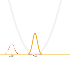
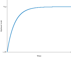
Figure 3. On the left, in dotted red, the initial data $f_{\varepsilon}(0,\cdot)$, and in orange the distribution $f_{\varepsilon}$ after a long time. In the background the selection function $m$ with a global optimum $z_{opt}$. On the right, the trajectory of the dominant trait $\operatorname{z_{\ast}}$.

Our framework encompasses more general selection functions with multiple local minima, as depicted in Figure 4. The condition in equation 1.14 restricts somehow the position of those minima. If one assumes that $\operatorname{z_{\ast}}$ starts from a local minimum, that is $m^{\prime}(\operatorname{z_{\ast}}(0))=0$, then this condition is that the selective difference between minima must be inferior to $1$ : $m(\operatorname{z_{\ast}}(0))-m(z_{opt})<1$. We recover the structural condition under which the analysis for the stationary case was performed, see Calvez et al., (2019).

The selection function depicted in Figure 4, coupled with $\operatorname{z_{\ast}}(0)$ verifies the condition equation 1.14. Then as stated by Theorem 1.4 the population density $f_{\varepsilon}$ concentrates around the local minimum, accordingly to the gradient flow dynamics of Assumption 1.1.

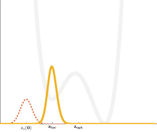
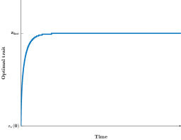
Figure 4. On the left, in dotted red, the initial data $f_{\varepsilon}(0,\cdot)$, and in orange the distribution $f_{\varepsilon}$ after a long time. In the background the selection function $m$ with a global optimum $z_{opt}$ and a local optimum $z_{loc}$. On the right, the trajectory of the dominant trait $\operatorname{z_{\ast}}$. The function $M$ is uniformly positive.

A case not taken into account by our methodology is when equation 1.14 is not verified at all times. This is the case if the slopes of the lines between local and global minima are too sharp. For instance, this is true in the case of Figure 5. Interestingly, what is observed is a critical behavior. The solution will first concentrate around the first local minimum before jumping sharply in the attraction basin of the global minimum see the right hand picture of Figure 5.

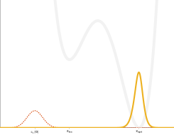
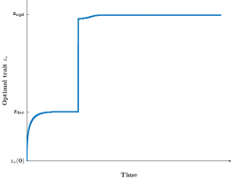
Figure 5. On the left, in dotted red, the initial data $f_{\varepsilon}(0,\cdot)$, and in orange the distribution $f_{\varepsilon}$ after a long time. In the background the selection function $m$ with a global optimum $z_{opt}$ and a local optimum $z_{loc}$. On the right, the trajectory of the dominant trait $\operatorname{z_{\ast}}$. The function $M$ is not uniformly positive.

Under this model it would seem that the population will concentrate around the global minimum of selection if it is much better than the other selective optima. Interestingly, the value of the local maximum in between the two minima, that could act as an obstacle between the two convex selection valleys, do not appear to play a role. On the other hand if the global minimum is not much better than a local minima, in the sense that each of them falls under the regime of equation 1.14, the population can concentrate around this local minimum.

Influence of the sign of $q_{\varepsilon}$. We introduced the scalar $q_{\varepsilon}$ in equation 1.18 as part of the decomposition of $U_{\varepsilon}$ between the affine parts and the rest of the function, which we later justified by heuristics on the linearized problem, see Table 1. We can propose a different interpretation of this scalar,related to the Gaussian distribution.

The logarithmic transform equation 1.2 coupled with the decomposition equation 1.18 can be rewritten as the following transform on the solution of equation $P_{t}f_{\varepsilon}$ :

(9.1) $$f_{\varepsilon}(t,z)=\frac{1}{\varepsilon\sqrt{2\pi}}\exp\left(\dfrac{\lambda(t)-\varepsilon^{2}p_{\varepsilon}(t)+\varepsilon^{4}q_{\varepsilon}(t)^{2}}{\varepsilon^{2}}-\dfrac{\Big{(}z-(\operatorname{z_{\ast}}(t)-\varepsilon^{2}q_{\varepsilon}(t))\Big{)}^{2}}{2\varepsilon^{2}}-V_{\varepsilon}(t,z)\right).$$

Therefore one can see that $q_{\varepsilon}$ is the correction to the mean of the Gaussian distribution at the next order in $\varepsilon$. Its sign corresponds to the sign of the error made on the mean of the Gaussian distribution. If $q_{\varepsilon}$ is positive, the correction of $\operatorname{z_{\ast}}$ lies on its left. This is consistent with the following reasoning on the limit value $q^{\ast}=\displaystyle~\lim_{\varepsilon\to 0}q_{\varepsilon}$, defined in equation 1.19. For clarity, suppose that $\operatorname{z_{\ast}}$ does not depend on time, that is the regime of the stationary case. Then from equation 1.19, we find an explicit value for $q^{\ast}$, which coincides with (Calvez et al.,, 2019, equation 3.2) :

$$q^{\ast}=\frac{m^{(3)}(\operatorname{z_{\ast}})}{2m^{\prime\prime}(\operatorname{z_{\ast}})}.$$

By local convexity of $m$ around $\operatorname{z_{\ast}}$, see equation 1.13, the sign of $q^{\ast}$ is the same than the sign of $m^{(3)}(\operatorname{z_{\ast}})$. Therefore, if this scalar is positive, selection leans the profile towards the left, which has better selective values than the right, since it is flatter. Therefore, we recover what we deduced from equation 9.1, the sign of $q_{\varepsilon}$ is linked to the skewness of the selection function $m$ around $\operatorname{z_{\ast}}$.

References

- Barfield et al., (2011) Barfield, M., Holt, R. D., and Gomulkiewicz, R. (2011). Evolution in Stage-Structured Populations. The American naturalist, 177(4):397–409.
- Barles et al., (2009) Barles, G., Mirrahimi, S., and Perthame, B. (2009). Concentration in Lotka-Volterra parabolic or integral equations: a general convergence result. Methods and Applications of Analysis, 16(3):321–340.
- Barles and Perthame, (2007) Barles, G. and Perthame, B. (2007). Concentrations and constrained hamilton-jacobi equations arising in adaptive dynamics. Contemporary Mathematics, 439:57–68.
- Barton et al., (2017) Barton, N., Etheridge, A., and Véber, A. (2017). The infinitesimal model: Definition, derivation, and implications. Theoretical population biology, 118:50–73.
- Bouin et al., (2019) Bouin, E., Bourgeron, T., Calvez, V., Cotto, O., Garnier, J., Lepoutre, T., and Ronce, O. (2019). Equilibria of quantitative genetics models beyond the gaussian approximation i: Maladaptation to a changing environment. In preparation.
- Bouin et al., (2018) Bouin, E., Garnier, J., Henderson, C., and Patout, F. (2018). Thin Front Limit of an Integro-differential Fisher-KPP Equation with Fat-Tailed Kernels. SIAM Journal on Mathematical Analysis, 50(3):3365–3394.
- Bulmer, (1980) Bulmer, M. G. (1980). The mathematical theory of quantitative genetics. Clarendon Press.
- Calvez et al., (2019) Calvez, V., Garnier, J., and Patout, F. (2019). Asymptotic analysis of a quantitative genetics model with nonlinear integral operator. Journal de l’École polytechnique — Mathématiques, 6:537–579.
- Calvez and Lam, (2018) Calvez, V. and Lam, K.-Y. (2018). Uniqueness of the viscosity solution of a constrained Hamilton-Jacobi equation. arXiv:1809.05317 [math]. arXiv: 1809.05317.
- Cotto and Ronce, (2014) Cotto, O. and Ronce, O. (2014). Maladaptation as a source of senescence in habitats variable in space and time. Evolution, 68(9):2481–2493.
- Diekmann et al., (2005) Diekmann, O., Jabin, P.-E., Mischler, S., and Perthame, B. (2005). The dynamics of adaptation: an illuminating example and a Hamilton-Jacobi approach. Theoretical Population Biology, 67(4):257–271.
- Fisher, (1918) Fisher, R. A. (1918). The correlation between relatives on the supposition of mendelian inheritance. Transactions of the Royal Society of Edinburgh, 52:399–433.
- Huisman and Tufto, (2012) Huisman, J. and Tufto, J. (2012). Comparison of non-gaussian quantitative genetic models for migration and stabilizing selection. Evolution: International Journal of Organic Evolution, 66(11):3444–3461.
- Kirkpatrick and Barton, (1997) Kirkpatrick, M. and Barton, N. H. (1997). Evolution of a species’ range. The American Naturalist, 150(1):1–23.
- Lorz et al., (2011) Lorz, A., Mirrahimi, S., and Perthame, B. (2011). Dirac mass dynamics in multidimensional nonlocal parabolic equations. Communications in Partial Differential Equations, 36(6):1071–1098.
- Mirrahimi, (2018) Mirrahimi, S. (2018). Singular limits for models of selection and mutations with heavy-tailed mutation distribution. arXiv preprint arXiv:1807.10475.
- Mirrahimi and Raoul, (2013) Mirrahimi, S. and Raoul, G. (2013). Dynamics of sexual populations structured by a space variable and a phenotypical trait. Theoretical population biology, 84:87–103.
- Mirrahimi and Roquejoffre, (2015) Mirrahimi, S. and Roquejoffre, J.-M. (2015). A class of Hamilton-Jacobi equations with constraint: uniqueness and constructive approach. arXiv:1505.05994 [math]. arXiv: 1505.05994.
- Méléard and Mirrahimi, (2015) Méléard, S. and Mirrahimi, S. (2015). Singular Limits for Reaction-Diffusion Equations with Fractional Laplacian and Local or Nonlocal Nonlinearity. Communications in Partial Differential Equations, 40(5):957–993.
- Perthame, (2007) Perthame, B. (2007). Transport equations in biology. Frontiers in mathematics. Birkhäuser, Basel.
- Raoul, (2017) Raoul, G. (2017). Macroscopic limit from a structured population model to the kirkpatrick-barton model. arXiv preprint arXiv:1706.04094.
- Roughgarden, (1972) Roughgarden, J. (1972). Evolution of niche width. The American Naturalist, 106(952):683–718.
- Slatkin, (1970) Slatkin, M. (1970). Selection and polygenic characters. Proceedings of the National Academy of Sciences, 66(1):87–93.
- Slatkin and Lande, (1976) Slatkin, M. and Lande, R. (1976). Niche Width in a Fluctuating Environment-Density Independent Model. The American Naturalist, 110(971):31–55.
- Tufto, (2000) Tufto, J. (2000). Quantitative genetic models for the balance between migration and stabilizing selection. Genetics Research, 76(3):285–293.
- Turelli, (2017) Turelli, M. (2017). Commentary: Fisher’s infinitesimal model: A story for the ages. Theoretical Population Biology, 118:46–49.
- Turelli and Barton, (1994) Turelli, M. and Barton, N. H. (1994). Genetic and statistical analyses of strong selection on polygenic traits: what, me normal? Genetics, 138(3):913–941.