Modular representations and reflection subgroups

Abstract.

The Hecke category is at the heart of several fundamental questions in modular representation theory. We emphasise the role of the “philosophy of deformations” both as a conceptual and computational tool, and suggest possible connections to Lusztig’s “philosophy of generations”. On the geometric side one can understand deformations in terms of localisation in equivariant cohomology. Recently Treumann and Leslie-Lonergan have added Smith theory, which provides a useful tool when considering mod $p$ coefficients. In this context, we make contact with some remarkable work of Hazi. Using recent work of Abe on Soergel bimodules, we are able to reprove and generalise some of Hazi’s results. Our aim is to convince the reader that the work of Hazi and Leslie-Lonergan can usefully be viewed as some kind of localisation to “good” reflection subgroups. These are notes for my lectures at the 2019 Current Developments in Mathematics at Harvard.

1. Introduction

The following notes revolve around modular representations of algebraic groups, symmetric groups and the Hecke category. There are already a number of surveys on this topic [JW17, Wil17a, AR18a, Wil18] and there is even a book on the way [EMTW19]. It would be silly to repeat this content. Instead I have tried to take a more speculative perspective, and to dream a little. The main inspiration is recent work of Treumann [Tre19], Hazi [Haz17], Abe [Abe19] and Leslie-Lonergan [LL18]. As I was finishing these notes I became aware of the work of McDonnell [McD19], which comes to similar conclusions to these notes. Our hope is that our account complements McDonnell’s.

Let us point out that these notes are rather inhomogeneous in their demands on the reader. §1 is introductory, and intended for a general audience. §2 assumes quite a lot of background from Lie theory. The material of §2 served as a principal motivation for the writing of these notes, and so we thought it would be unfortunate not to include it. §3 and §4 are more accessible. The road gets steeper in §5 and steeper still in §6, where I am writing for experts.

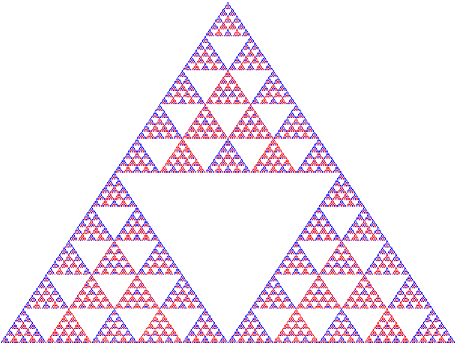
Figure 1. A little mystery.

1.1. A mystery

The reader is asked to contemplate the picture in Figure 1. What could it be? It is appears to be some Sierpiński like figure, but we promise the reader that there is a little more going on. For example, the colours have a meaning. In Figure 2 one has a close up, as well as a close up of a related picture.

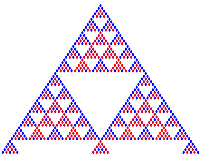
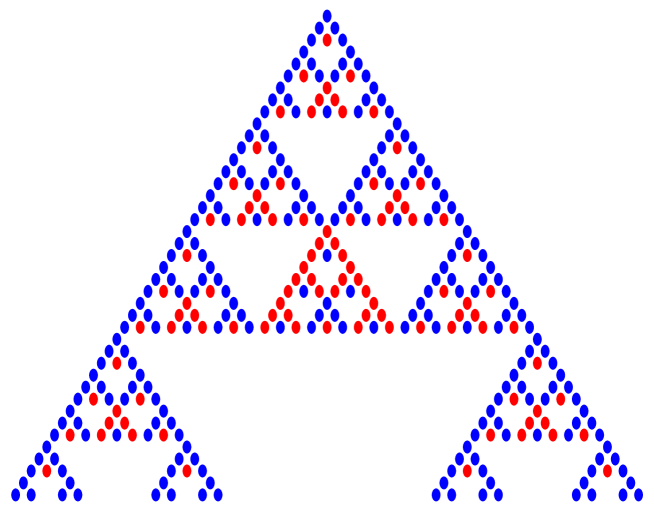
Figure 2. Close ups, for $p=5$ (top) and $p=3$ (bottom).

Remark 1.1.

From the zoomed in pictures it is clear that the apparent fractal nature of Figure 1 actually terminates as we zoom in.

The answer is that we are staring at Pascal’s triangle. More precisely, we are staring at Pascal’s triangle modulo $p$, for $p=3$ and $5$. The (non-trivial) colours encode the (non-trivial) residue classes modulo $p$:

$$\begin{array}[]{c}\leavevmode\hbox to82.8pt{\vbox to70.02pt{\text{[drawing]}}}\end{array}\stackrel{{\scriptstyle\text{mod $3$}}}{{\longrightarrow}}\begin{array}[]{c}\leavevmode\hbox to82.8pt{\vbox to70.02pt{\text{[drawing]}}}\end{array}=\begin{array}[]{c}\includegraphics[width=85.35826pt]{pics/cp3zoomzoom}\end{array} 1 1 1 1 2 1 1 3 3 1 1 4 6 4 1 1 5 10 10 5 1 1 1 1 1 2 1 1 0 0 1 1 1 0 1 1 1 2 1 1 2 1 1 1 1 1 2 1 1 3 3 1 1 4 6 4 1 1 5 10 10 5 1 1 1 1 1 2 1 1 0 0 1 1 1 0 1 1 1 2 1 1 2 1$$

1.2. Modular representations

What on earth does this have to do with modular representations and reflection subgroups, the title of these notes? To begin explaining the connection, we start with one of the most fundamental of all groups

$$G=\operatorname{SL}_{2}$$

which we view as an algebraic group over $\Bbbk=\overline{{\mathbb{F}}}_{p}$, an algebraic closure of the finite field with $p$ elements. The reader can think of $G$ as being the collection of $2\times 2$-matrices

$$\left\{\left(\begin{matrix}a&b\\ c&d\end{matrix}\right)\in\operatorname{Mat}_{2}(\Bbbk)\;\middle|\;ad-bc=1\right\}.$$

A key feature in characteristic $p$ is the Frobenius endomorphism:

$$\operatorname{Fr}:\operatorname{SL}_{2} \rightarrow\operatorname{SL}_{2}$$

$$\left(\begin{matrix}a&b\\ c&d\end{matrix}\right) \mapsto\left(\begin{matrix}a^{p}&b^{p}\\ c^{p}&d^{p}\end{matrix}\right)$$

Nothing like this exists in characteristic $0$. It can be thought of as a kind of “everywhere contracting mapping”.

The questions in these notes are motivated by the study of algebraic representations of groups like $\operatorname{SL}_{2}$. This means we are studying homomorphisms

$$\rho:\operatorname{SL}_{2}\rightarrow\operatorname{GL}(V)$$

for some $\Bbbk$-vector space $V$, which are defined by polynomials in $a,b,c$ and $d$. One of the first results in the theory is that all representations are direct limits of finite-dimensional representations, so we usually assume that $V$ is finite-dimensional. In other words, we are studying polynomial homomorphisms into $GL_{n}$.

Remark 1.2.

If the reader is like the author, they might initially find the study of algebraic representations somewhat artificial. Why not stick to finite groups like $\operatorname{SL}_{2}({\mathbb{F}}_{q})$? In fact there is a close connection between representations of finite groups of Lie type like $\operatorname{SL}_{2}({\mathbb{F}}_{q})$ in “their own” characteristic, and the theory of algebraic representations. It turns out that the extra structures arising from the theory of algebraic groups are tremendously useful. One can think of the finite groups $\operatorname{SL}_{2}({\mathbb{F}}_{q})$ as somewhat like lattices in the “Lie group” $\operatorname{SL}_{2}$. Thus the passage from $\operatorname{SL}_{2}({\mathbb{F}}_{q})$ to $\operatorname{SL}_{2}$ is akin to the more familiar fact that the representation theory of connected Lie groups is easier than that of finite groups.

1.3. Some examples of algebraic representations

Here are a few examples of representations (of dimensions $1$, $2$ and $3$):

$$\left(\begin{matrix}a&b\\ c&d\end{matrix}\right) \mapsto(1)$$

$$\left(\begin{matrix}a&b\\ c&d\end{matrix}\right) \mapsto\left(\begin{matrix}a&b\\ c&d\end{matrix}\right)$$

$$\left(\begin{matrix}a&b\\ c&d\end{matrix}\right) \mapsto\left(\begin{matrix}a^{2}&ab&b^{2}\\ 2ac&ad+bc&2bd\\ c^{2}&cd&d^{2}\end{matrix}\right)$$

The first is the trivial representation. The second is the “natural representation”, so called because it arises from the definition of $\operatorname{SL}_{2}$ as a matrix group. The third arises as follows. The natural representation gives us a linear action of $\operatorname{SL}_{2}$ on

$$\operatorname{SL}_{2}\hskip 2.84526pt\lefttorightarrow\hskip 2.84526ptV=\Bbbk X\oplus\Bbbk Y.$$

For example,

$$\left(\begin{matrix}a&b\\ c&d\end{matrix}\right)\cdot X=aX+cY.$$

Thus $\operatorname{SL}_{2}$ also acts on the second symmetric power

$$\operatorname{SL}_{2}\hskip 2.84526pt\lefttorightarrow\hskip 2.84526ptS^{2}(V)=\Bbbk X^{2}\oplus\Bbbk XY\oplus\Bbbk Y^{2}.$$

Writing out this action in the basis of monomials produces the above matrices. For example

$$\left(\begin{matrix}a&b\\ c&d\end{matrix}\right)\cdot X^{2}=(aX+cY)^{2}=a^{2}X+2acXY+c^{2}Y^{2}$$

which is the first column of our matrix. (This also makes it clear why our third representation above is actually a representation, which is not clear when presented with a formula.)

1.4. Chevalley’s theorem

Of course there was no reason to stop at the second symmetric power above. We can consider the module

$$\operatorname{SL}_{2}\hskip 2.84526pt\lefttorightarrow\hskip 2.84526pt\nabla_{n}:=S^{n}V=\Bbbk X^{n}\oplus\Bbbk X^{n-1}Y\Bbbk\oplus\dots\oplus\Bbbk Y^{n}$$

for any $n\geq 0$. The modules $\nabla_{0},\nabla_{1}$ and $\nabla_{2}$ being the cases considered above. We have

$$\dim\nabla_{n}=n+1.$$

If our field were of characteristic zero, these modules would provide a complete list of inequivalent irreducible representations of $\operatorname{SL}_{2}$.

However, in the current setting the situation is a little more interesting. Let us for concreteness assume that $p=3$, and consider

$$\nabla_{3}=\Bbbk X^{3}\oplus\Bbbk X^{2}Y\oplus\Bbbk XY^{2}\oplus\Bbbk Y^{3}.$$

If we act on the vector $X^{3}\in\nabla_{3}$ we have

$$\left(\begin{matrix}a&b\\ c&d\end{matrix}\right)\cdot X^{3}=(aX+cY)^{3}=a^{3}X^{3}+c^{3}Y^{3}$$

by the “Freshman’s dream” in characteristic 3. A similar calculation for $Y^{3}$ shows that

$$\Bbbk X^{2}\oplus\Bbbk Y^{3}\subset\nabla_{3}$$

is a non-trivial $\operatorname{SL}_{2}$-invariant submodule. Moreover, this submodule affords the representation

$$\left(\begin{matrix}a&b\\ c&d\end{matrix}\right)\mapsto\left(\begin{matrix}a^{3}&b^{3}\\ c^{3}&d^{3}\end{matrix}\right)$$

obtained by pulling the natural module back along the Frobenius morphism $\operatorname{Fr}$ from earlier. This operation on representations is called Frobenius twist and is fundamental to the theory.

It turns out that $\nabla_{n}$ always has a unique simple submodule. Moreover, if we denote this submodule by $L_{n}\subset\nabla_{n}$ then we have a bijection:

$${\mathbb{Z}}_{\geq 0} \stackrel{{\scriptstyle\sim}}{{\rightarrow}}\left\{\begin{array}[]{c}\text{simple algebraic}\\ \operatorname{SL}_{2}\text{-modules}\end{array}\right\}_{/\cong}$$

$$n \mapsto\hskip 42.67912ptL_{n}$$

Remark 1.3.

This is a example of Chevalley’s theorem, which is true for any reductive algebraic group. In the context of a general algebraic group it tells us that simple modules are always classified by highest weight, just as over ${\mathbb{C}}$. (The reader is cautioned that although they are classified independently of $p$, their structure varies subtly based on $p$.)

1.5. Characters

Inside $\operatorname{SL}_{2}$ we can consider the maximal torus

$$T:=\left\{\left(\begin{matrix}a&0\\ 0&a^{-1}\end{matrix}\right)\right\}\subset\operatorname{SL}_{2}.$$

Any algebraic representation $V$ of $\operatorname{SL}_{2}$ splits as a direct sum

$$V=\bigoplus_{m\in{\mathbb{Z}}}V_{m}$$

of its weight spaces

$$V_{m}:=\left\{v\in V\;\middle|\;\left(\begin{matrix}a&0\\ 0&a^{-1}\end{matrix}\right)\cdot v=a^{m}v\text{ for all $a\in\Bbbk^{*}$}\right\}.$$

Probably the most basic invariant of a representation aside from its dimension is its character

$$\operatorname{ch}(V):=\sum_{m\in{\mathbb{Z}}}(\dim V_{m})e^{m}\in{\mathbb{Z}}_{\geq 0}[e^{\pm 1}].$$

For example, $X^{i}Y^{n-i}\in\nabla_{n}$ satisfies

$$\left(\begin{matrix}a&0\\ 0&a^{-1}\end{matrix}\right)\cdot X^{i}Y^{n-i}=a^{i}a^{i-n}X^{i}Y^{n-i}=a^{-n+2i}X^{i}Y^{n-i}.$$

Thus all weight spaces of $\nabla_{n}$ are either 0 or 1-dimensional and

$$\operatorname{ch}(\nabla_{n})=e^{-n}+e^{-n+2}+\dots+e^{n-2}+e^{n}=\frac{e^{n}-e^{-n-2}}{1-e^{-2}}.$$

Remark 1.4.

The last equality is an example of Weyl’s character formula, which is of central importance in the theory of compact Lie groups, as it is to the theory of algebraic groups over ${\mathbb{C}}$. It is also very important in the theory we consider here, as it gives us the characters of certain building blocks of all representations (so-called Weyl modules and induced modules, of which $\nabla_{n}$ is an example).

1.6. Characters of simples

Let us assume $p=3$. A few lines of calculations give the following descriptions of $L_{n}\subset\nabla_{n}$ for $n=0,1,\dots,6$:

The third line is our calculation using the Freshman’s dream from earlier. Thus the characters (for $n=0,1,\dots,6$ as earlier) are given as follows:

This should remind the reader of the picture earlier:

$$\begin{array}[]{c}\includegraphics[width=341.43306pt]{pics/cp3}\end{array}$$

This is not an accident: the non-zero $(n-2i)^{th}$ weight space in $L_{n}$ is non-zero (hence one-dimensional), if and only $n\choose i$ is non-zero modulo $p$.

1.7. Steinberg tensor product theorem

Let us continue our running example of $p=3$. We have seen that

(1) $$\nabla_{0},\nabla_{1},\nabla_{2}$$

are simple, but that $\nabla_{3}$ is not. In fact, we saw that it contains a two-dimensional submodule $L_{3}$ which is isomorphicto a Frobenius twist

$$L_{3}\cong\nabla_{1}^{(1)}\subset\nabla_{3}.$$

where $V\mapsto V^{(m)}$ denotes the operation of precomposing $m$ times with the Frobenius map.

In fact, our three modules (1) above are the building blocks of any representation. Given $m$ we consider its $3$-adic expansion

$$m=\sum_{i=1}^{\ell}m_{i}p^{i}\quad\text{with $0\leq m_{i}<3$}$$

and we have

(2) $$L_{m}:=\nabla_{m_{0}}\otimes\nabla_{m_{1}}^{(1)}\otimes\dots\otimes\nabla_{m_{\ell}}^{(\ell)}.$$

More precisely, one has an evident map given by multiplication from the above into $\nabla_{m}$, and the claim is that its image is simple.

Of course there is nothing special about $p=3$. For general $p$ we consider its $p$-adic expansion

$$m=\sum_{i=1}^{\ell}m_{i}p^{i}\quad\text{with $0\leq m_{i}<p$}$$

and the above tensor decomposition holds. Taking characters this implies

$$\operatorname{ch}(L_{m})=\prod_{i=1}^{\ell}(e^{-m_{i}}+e^{-m_{i}+2}+\dots+e^{m_{i}-2}+e^{m_{i}})^{(i)}$$

where $f\mapsto f^{(i)}$ is induced by the map $e\mapsto e^{p^{i}}$ on ${\mathbb{Z}}[e^{\pm 1}]$.

Remark 1.5.

The reader can use this formula to check that the $(n-2i)^{th}$ weight space of $L_{m}$ is non-zero if and only if there are no carries when $i$ and $m$ are added $p$-adically, which is the condition for the binomial coefficient $n\choose i$ to be non-zero, by Kummer’s theorem on valuations of binomial coefficients.

Remark 1.6.

Equation (2) is an instance of the Steinberg tensor product theorem, which is valid for any reductive group. For a general group however, the question of the description of the building blocks ($\nabla_{0},\dots,\nabla_{p-1}$ for $\operatorname{SL}_{2}$) is much more complicated. This is the subject of Lusztig’s character formula [Lus80, Wil17a, Lus15].

1.8. Generations

It is interesting to consider Pascal’s triangle, where we replace the binomial coefficients with their Gaußian cousins

(3) $${n\choose i}\rightsquigarrow\left[\begin{matrix}n\\ i\end{matrix}\right]_{v}:=\frac{[n]_{v}![n-1]_{v}!\dots[n-i+1]_{v}!}{[i]_{v}![i-1]_{v}!\dots[2]_{v}![1]_{v}!}\in{\mathbb{Z}}[v^{\pm 1}].$$

where

(4) $$\small[n]_{v}!=[n]_{v}[n-1]_{v}\dots[2]_{v}[1]_{v}=\frac{v^{n}-v^{-n}}{v-v^{-1}}\cdot\frac{v^{n-1}-v^{-n+1}}{v-v^{-1}}\cdot\dots\cdot(v+v^{-1})\cdot 1.$$

That is we replace

$$\tiny\begin{array}[]{c}\leavevmode\hbox to70.32pt{\vbox to110.41pt{\text{[drawing]}}}\end{array}\rightsquigarrow\tiny\begin{array}[]{c}\leavevmode\hbox to215.41pt{\vbox to110.98pt{\text{[drawing]}}}\end{array} 1 1 1 1 2 1 1 3 3 1 1 4 6 4 1 1 5 10 10 5 1 \vdots \vdots \vdots 1 1 1 1 [2]_{v} 1 1 [3]_{v} [3]_{v} 1 1 [4]_{v} [3]_{v}[2]_{v^{2}} [4]_{v} 1 1 [5]_{v} [5]_{v}[2]_{v^{2}} [5]_{v}[2]_{v^{2}} [5]_{v} 1 \vdots \vdots \vdots 1 1 1 1 2 1 1 3 3 1 1 4 6 4 1 1 5 10 10 5 1 \vdots \vdots \vdots 1 1 1 1 [2]_{v} 1 1 [3]_{v} [3]_{v} 1 1 [4]_{v} [3]_{v}[2]_{v^{2}} [4]_{v} 1 1 [5]_{v} [5]_{v}[2]_{v^{2}} [5]_{v}[2]_{v^{2}} [5]_{v} 1 \vdots \vdots \vdots$$

It has been observed in several circumstances that Gaußian binomial coefficients at a $p^{th}$-root of unity “imitate characteristic $p$.” (This observation goes back at least to [Lus89].) We can see this here: if we specialise $v:=e^{{2\pi i}/3}$ we get a vanishing behaviour that looks like the “first level” of the picture that we began with (for clarity we have replaced zeroes with empty space):

From the perspective of these notes, the most important thing to notice about this picture is that its vanishing behaviour approximates the earlier pictures, but is markedly simpler.

There exists an object (Lusztig’s form of the quantum group of $\mathfrak{sl}_{2}$ specialised at a $p^{th}$-root of unity) whose simple modules have characters determined by the vanishing behaviour in the above picture. This is a shadow of the fact that the quantum group at a root of unity imitates the representation theory of a reductive algebraic group in characteristic $p$, but is simpler.

Remark 1.7.

The analogue of the questions discussed in this note for quantum group was discussed by Wolfgang Soergel at the Current Developments in 1997. (More precisely, due to the intervention of a border agent they were not discussed; but that is another story. However the notes are available [Soe99].)

1.9. Themes of these notes

This discussion of $\operatorname{SL}_{2}$ is intended to suggest two themes, which are major motivations for the considerations in these notes.

Self-similarity: We expect fractal-like behaviour in modular representation theory; both on a numerical level (dimensions, characters); and on a categorical level. This behaviour is often tied to the Frobenius endomorphism

$$\operatorname{Fr}:G\rightarrow G$$

which implies that the category of representations of $G$ is self-similar. Indeed, it contains copies of itself given by the essential images of the Frobenius twist and their variants. We suggest that this similarity is connected to the self-similarity of affine Weyl groups, which contain many isomorphic copies of themselves.

Philosophy of generations: We seek “blueprints” for the fractal-like behaviour, which behave in a simpler fashion. The archetypal example of this is Pascal’s triangle for Gaußian binomial coefficients, discussed in the previous section. These often involve deformations of our categories (either over polynomial rings, or to characteristic 0). This philosophy has first been enunciated by Lusztig [Lus15], where he shows that simple characters display a “generational behaviour”. It is also pursued in [LW18b, LW18a] for tilting characters, where it is a very useful guiding principle. Despite its usefulness, we still lack a rigorous definition of generations (aside from the case of quantum groups at roots unity, which provide “generation 1”). A second aim of these notes is to point out that the self-similarity of affine Weyl groups suggests a possible approach to a rigorous definition.

Remark 1.8.

(Highly speculative!) Following on from Remark 1.1 one can hope to replace $G$ with an object which has simple characters displaying a genuinely fractal nature. It seems likely that such an object is given by the projective limit

$$\hat{G}:=\lim_{\leftarrow}G$$

over the tower of Frobenius maps. I believe this is a perfectoid space in Scholze’s sense [Sch13]. At least one can make a sensible guess as to what its algebra of distributions is, and study its representation theory that way. Its representation theory is potentially tied to the generic cohomology of [CPSvdK77].

2. Philosophy of deformations

In the following I will try to explain the philosophy of deformations as it applies to representation theory, and give a few examples.

2.1. Deformations

The notion of deformation is fundamental to algebraic geometry. We are particularly interested in deformations relating smooth and singular varieties. This is encapsulated in the classic picture

of a smooth affine conic degenerating to a singular one. In algebraic geometry the relationship between smooth and singular goes both ways. For example, smooth varieties are used to construct interesting objects on singular varieties (e.g. “vanishing cycles”), or singular varieties are used to understand smooth varieties (e.g. in the Gross-Siebert program in mirror symmetry).

One can draw a similar picture in the modular representation theory of finite groups. Consider a finite group $G$. Then one can think of $\operatorname{Rep}{\mathbb{Z}}G$ as being a family of categories lying over the line $\operatorname{Spec}{\mathbb{Z}}$ with generic fibre $\operatorname{Rep}{\mathbb{Q}}G$ (which is semi-simple, therefore “smooth”) and other fibres $\operatorname{Rep}{\mathbb{F}}_{p}G$ (which is never of finite homological dimension if $p$ divides the order of $G$, and is therefore “singular” at these points):

The reader is cautioned not to take this picture literally. A slightly more accurate picture would have finitely many reduced points (the simple representations of $G$ over ${\mathbb{Q}}_{p}$) degenerating to some complicated non-reduced scheme at the singular fibre. In representation theory the flow of information is almost always from the “smooth” to the “singular”.

The above setting of modular representations of finite groups is extraordinarily complicated, and there are few groups where we understand well what happens at the “singular fibre”. However quantum objects (Hecke algebras, quantum groups) give us simpler problems which we can attempt to study (both for their own interest, and in the hope that they may shed some light on modular representation theory).

2.2. The Hecke algebra

The simplest example of this phenomenon is the Hecke algebra of the symmetric group. Recall that the symmetric group $S_{n}$ has a presentation with generators the $i^{th}$ simple transposition $s_{i}=(i,i+1)$, for $i=1,\dots,n-1$, and relations:

(5) $$s_{i}^{2} =\operatorname{id},$$

(6) $$s_{i}s_{i+1}s_{i} =s_{i+1}s_{i}s_{i+1},$$

(7) $$s_{i}s_{j} =s_{j}s_{i}\qquad\text{if $|i-j|>1$}.$$

The Hecke algebra $\textrm{H}_{S_{n}}$ of the symmetric group is a ${\mathbb{Z}}[v^{\pm 1}]$-algebra with generators $\delta_{i}$, for $i=1,\dots,n-1$, and relations:

(8) $$\delta_{i}^{2} =(v^{-1}-v)\delta_{i}+1,$$

(9) $$\delta_{i}\delta_{i+1}\delta_{i} =\delta_{i+1}\delta_{i}\delta_{i+1},$$

(10) $$\delta_{i}\delta_{j} =\delta_{j}\delta_{i}\qquad\text{if $|i-j|>1$}.$$

Setting $v=1$ we recover the relations of the symmetric group. The Hecke algebra is free over ${\mathbb{Z}}[v^{\pm 1}]$ with a “standard basis” $\{\delta_{x}\;|\;x\in S_{n}\}$, which becomes the standard basis of the group algebra when we specialise $v:=1$. It is useful to think of the Hecke algebra as a flat deformation of the group algebra of the symmetric group over $\operatorname{Spec}{\mathbb{Z}}[v^{\pm 1}]$.

In the group algebra of $S_{n}$ one has the central element

$$e=\sum_{x\in S_{n}}x$$

which satisfies

(11) $$e^{2}=|S_{n}|\cdot e=n!\cdot e.$$

One can use this to show that $kS_{n}$ is semi-simple if and only if $n!$ is non-zero in $k$.

The analogue in $\textrm{H}_{S_{n}}$ of $e$ is

$$e_{v}=\sum_{x\in S_{n}}v^{N-\ell(x)}\delta_{x}$$

where $\ell$ is the usual length a permutation, and $N=n(n-1)/2$ is the length of the permutation that switches $1$ and $n$, $2$ and $n-1$, etc. The analogue of (11) is

(12) $$e_{v}^{2}=[n]_{v}!\cdot e_{v}.$$

where $[n]_{v}!$ is as in (4). Similarly to the case of $S_{n}$, one can use (11) to show that, for any field and non-zero $\lambda\in k$, the specialisation (“fibre”) $\textrm{H}_{S_{n}}\otimes_{v\mapsto\lambda}k$ is semi-simple if and only if the evaluation of $[n]_{v}!$ at $v=\lambda$ is non-zero in $k$. If we specialise $v\mapsto\lambda\in{\mathbb{C}}$ then we deduce from (4) that $\textrm{H}_{S_{n}}\otimes_{v\mapsto\lambda}{\mathbb{C}}$ is semi-simple if and only if $\lambda$ is not an $m^{th}$-root of unity, for $m=2,\dots,n$.

Now $\operatorname{Spec}{\mathbb{Z}}[v^{\pm 1}]$ is of dimension 2 and hence has two directions: a “geometric” direction (corresponding to specialisations of $v$); and an “arithmetic” direction (corresponding to specialisations of ${\mathbb{Z}}$ to various fields. There has been significant progress in our understanding of the geometric direction (e.g. the LLT conjecture [LLT96], proved by Ariki [Ari96]). Progress in the arithmetic direction has been more modest, but the picture with Hecke algebras has been a fruitful source of problems and motivation (e.g. the James conjecture [Jam90, Wil17b]).

2.3. Higher-dimensional bases

In algebraic geometry one also encounters deformations over higher dimensional bases. It is a fundamental observation (developed by Jantzen [Jan79], Gabber-Joseph [GJ81], Soergel [Soe92], …) that a similar picture exists in the infinite-dimensional representation theory of complex semi-simple Lie algebras.

Let $\mathfrak{g}$ denote a complex semi-simple Lie algebra, with Cartan and Borel subalgebra ${\mathfrak{h}}\subset{\mathfrak{b}}\subset\mathfrak{g}$, root system $\Phi\subset{\mathfrak{h}}^{*}$ and Weyl group $W$. Let ${\mathcal{O}}$ denote the BGG category of certain infinite-dimensional representations of $\mathfrak{g}$. Recall that we have a decomposition via central character

$${\mathcal{O}}=\bigoplus_{\lambda\in{\mathfrak{h}}^{*}/(W\cdot)}{\mathcal{O}}_{\lambda}$$

and the most complicated pieces are ${\mathcal{O}}_{\lambda}$, where $\lambda$ is dominant integral.

Let us fix $\lambda$, and suppose we wish to study ${\mathcal{O}}_{\lambda}$. Deformed category ${\mathcal{O}}$ defines a deformation of ${\mathcal{O}}_{\lambda}$ over $\operatorname{Spec}\hat{R}$, where $\hat{R}$ denotes the completion of the symmetric algebra on ${\mathfrak{h}}$ at the maximal ideal generated by the point $\lambda$; it should be thought of as an infinitesimal neighbourhood of $\lambda\in{\mathfrak{h}}^{*}$. The picture of the fibres of deformed category ${\mathcal{O}}$ are as follows:

Here we have drawn the picture for ${\mathfrak{sl}}_{3}$. The lines in $\operatorname{Spec}\hat{R}$ are the root hyperplanes passing through $\lambda$. The fibres are as follows:

1. ${\mathcal{O}}_{\lambda}$ is the fibre over the central point; it is the category that we are interested in.

2. ${\mathcal{O}}_{{\mathfrak{sl}}_{2}}$ is the fibre over all points that lie in precisely one root hyperplane. Each such fibre is equivalent to a direct sum of blocks of category ${\mathcal{O}}$ for ${\mathfrak{sl}}_{2}({\mathbb{C}})$.

3. ${\mathcal{O}}_{\mathrm{gen}}$ is the fibre over points which do not lie on any root hyperplane. Each such fibre is a semi-simple category, equivalent to $|W|$ copies of the category of finite-dimensional ${\mathbb{C}}$-vector spaces.

The reason why this picture is so powerful is that it allows one to see ${\mathcal{O}}_{\lambda}$ (a very complicated category) as glued together out of simple categories (copies of vector spaces, and categories ${\mathcal{O}}$ for ${\mathfrak{sl}}_{2}$, which may be described explicitly).

Remark 2.1.

A similar setting occurs in the localisation theorem in equivariant cohomology, where the cohomology injects into equivariant cohomology of fixed points, with image described by conditions coming from one-dimensional orbits. This similarity is more than a coincidence and has been exploited in Soergel’s work.

Remark 2.2.

This example may appear unrelated to the earlier examples from modular representation theory. In fact, the examples from modular representation theory were an important motivation for Jantzen to introduce deformed category ${\mathcal{O}}$: he was seeking a way to apply the ideas from his study of Weyl modules in characteristic $p$ (and in particular their Jantzen filtrations) to category ${\mathcal{O}}$.

2.4. The anti-spherical category

In this section we discuss the various localisations of the anti-spherical category. The goal is to try to understand the anti-spherical category via the philosophy of deformations.

Remark 2.3.

The case of the anti-spherical module was the principle motivating example when writing these notes. We thus feel it is important not to defer the discussion of this case until the very end, which would perhaps be logical from a mathematical perspective. The discussion of this section is necessarily more technical than the previous sections. The reader unfamiliar with the Hecke category should defer the reading of this section until they have read the section on the Hecke category. It would also be very helpful to have read the introductions of [RW18] and [LW].

Let ${\mathcal{H}}$ denote the Hecke category of an affine Weyl group $W$. As a right module over itself it is linear over $R$, where $R$ denotes the symmetric algebra on ${\mathscr{X}}_{\mathrm{rot}}$, the characters of the extended torus

$$T_{\mathrm{rot}}:=T\times{\mathbb{C}}^{*}_{\mathrm{rot}}$$

where $T$ is a maximal torus of a reductive group $G$, and ${\mathbb{C}}^{*}_{\mathrm{rot}}$ is the loop rotation ${\mathbb{C}}^{*}$ inside the loop group ${\mathbb{C}}^{*}_{\mathrm{rot}}\ltimes G((t))$. Thus we have

$${\mathscr{X}}_{\mathrm{rot}}:={\mathbb{Z}}\delta\oplus{\mathscr{X}}$$

where ${\mathscr{X}}$ denotes the character lattice of $T$. Here $\delta$ (which will play a crucial role below), is the identity character of the loop rotation ${\mathbb{C}}^{\times}_{\mathrm{rot}}\subset T_{\mathrm{rot}}$.

Let us consider the Hecke category ${\mathcal{H}}_{{\mathbb{Z}}_{p}}$ over the $p$-adic integers ${\mathbb{Z}}_{p}$. The anti-spherical module is by definition the quotient of additive categories

$${\mathcal{A}}:={\mathcal{H}}_{{\mathbb{Z}}_{p}}/\langle B_{w}\;|\;w\notin{}^{f}W\rangle_{\oplus}$$

where ${}^{f}W$ denotes minimal coset representatives for the right action of the finite Weyl group $W_{f}$. This is naturally a right ${\mathcal{H}}_{{\mathbb{Z}}_{p}}$-module, as $\langle B_{w}\;|\;w\notin{}^{f}W\rangle_{\oplus}$ is an ideal. (We have not covered all notation, see [RW18, §1.3] for more details.)

When we form this quotient we are forced to kill certain symmetries of ${\mathcal{H}}_{{\mathbb{Z}}_{p}}$. For example, if $\alpha_{s}\in{\mathscr{X}}$ denotes a simple root then $\alpha_{s}$ (viewed as an endomorphism of ${\mathcal{H}}$) factors through $B_{s}$, and hence is zero in ${\mathcal{A}}$. Hence all of ${\mathscr{X}}$ necessarily acts by zero. If we denote by $\mathbb{1}_{{\mathcal{A}}}$ the image of the unit in ${\mathcal{H}}_{{\mathbb{Z}}_{p}}$ in ${\mathcal{A}}$, then it turns out that

(13) $$\operatorname{End}^{\bullet}(\mathbb{1}_{{\mathcal{A}}})={\mathbb{Z}}_{p}[\delta]$$

where $\delta$ has degree 2. (In other words, the obvious endomorphisms $\alpha_{s}$ just discussed are killed, and the rest survives.)

Figure 3. Localisations and specialisations of ${\mathcal{A}}$.

$$\begin{array}[]{c}\leavevmode\hbox to347.82pt{\vbox to249.97pt{\text{[drawing]}}}\end{array} {\mathbb{F}}_{p}[\delta^{\pm 1}]\otimes_{{\mathbb{Z}}_{p}[\delta]}{\mathcal{A}} \cong \bigoplus_{x\in{}^{r}W}{\mathbb{F}}_{p}[\delta^{\pm 1}]\otimes_{{\mathbb{Z}}_{p}[\delta]}{\mathcal{A}}_{x} {\mathbb{Q}}_{p}[\delta^{\pm 1}]\otimes_{{\mathbb{Z}}_{p}[\delta]}{\mathcal{A}} \cong \bigoplus_{x\in{}^{f}W}{\mathbb{Q}}_{p}[\delta^{\pm 1}]-\textrm{mod} {\mathbb{F}}_{p}\otimes_{{\mathbb{Z}}_{p}[\delta]}{\mathcal{A}} \cong \mathrm{Tilt}_{0}(G^{\vee}_{{\mathbb{F}}_{p}}) {\mathbb{Q}}_{p}\otimes_{{\mathbb{Z}}_{p}[\delta]}{\mathcal{A}} \cong \mathrm{Tilt}_{0}(U_{\epsilon}(\mathfrak{g}^{\vee})) {\mathbb{F}}_{p} {\mathbb{Q}}_{p} \delta\neq 0 \delta=0 {\mathbb{F}}_{p}[\delta^{\pm 1}]\otimes_{{\mathbb{Z}}_{p}[\delta]}{\mathcal{A}} \cong \bigoplus_{x\in{}^{r}W}{\mathbb{F}}_{p}[\delta^{\pm 1}]\otimes_{{\mathbb{Z}}_{p}[\delta]}{\mathcal{A}}_{x} {\mathbb{Q}}_{p}[\delta^{\pm 1}]\otimes_{{\mathbb{Z}}_{p}[\delta]}{\mathcal{A}} \cong \bigoplus_{x\in{}^{f}W}{\mathbb{Q}}_{p}[\delta^{\pm 1}]-\textrm{mod} {\mathbb{F}}_{p}\otimes_{{\mathbb{Z}}_{p}[\delta]}{\mathcal{A}} \cong \mathrm{Tilt}_{0}(G^{\vee}_{{\mathbb{F}}_{p}}) {\mathbb{Q}}_{p}\otimes_{{\mathbb{Z}}_{p}[\delta]}{\mathcal{A}} \cong \mathrm{Tilt}_{0}(U_{\epsilon}(\mathfrak{g}^{\vee})) {\mathbb{F}}_{p} {\mathbb{Q}}_{p} \delta\neq 0 \delta=0$$

The crucial equality (13) allows us to view ${\mathcal{A}}$ as a family over the two-dimensional base ${\mathbb{Z}}_{p}[\delta]$. Figure 3 depicts the various localisations and specialisations of ${\mathcal{A}}$. Here are some more details:

1. (${\mathbb{Z}}_{p}[\delta]\rightsquigarrow{\mathbb{F}}_{p}$): This is the source of our interest in ${\mathcal{A}}$. Let $G^{\vee}_{{\mathbb{F}}_{p}}$ denote the (split) Langlands dual group over ${\mathbb{F}}_{p}$, and let $\mathrm{Tilt}_{0}(G^{\vee}_{{\mathbb{F}}_{p}})$ denote the full subcategory of tilting modules in the same block as the trivial module (the “principal block”). We have a functor

   $$\phi:{\mathbb{F}}_{p}\otimes_{{\mathbb{Z}}_{p}[\delta]}{\mathcal{A}}\rightarrow\mathrm{Tilt}_{0}(G^{\vee}_{{\mathbb{F}}_{p}})$$

   which satisfies $\phi\circ[1]\cong\phi$ and

   $$\phi:\bigoplus_{m\in{\mathbb{Z}}}\operatorname{Hom}({\mathcal{E}},{\mathcal{F}}[m])\stackrel{{\scriptstyle\sim}}{{\rightarrow}}\operatorname{Hom}(\phi({\mathcal{E}}),\phi({\mathcal{F}})).$$

   (In other words, $\phi$ induces an equivalence between $\mathrm{Tilt}_{0}(G^{\vee}_{{\mathbb{F}}_{p}})$ and the anti-spherical module specialised over ${\mathbb{F}}_{p}$ with $\delta=0$, once we forget the grading on the latter.) This allows one to deduce a character formula for tilting modules in terms of the $p$-Kazhdan-Lusztig basis.

2. (${\mathbb{Z}}_{p}[\delta]\rightsquigarrow{\mathbb{Q}}_{p}$): Let $\mathfrak{g}^{\vee}$ denote the complex semi-simple Lie algebra which is Langlands dual to $G$. Let $U_{\epsilon}(\mathfrak{g}^{\vee})$ denote the quantum group at a $p^{th}$ root of $1$ and let $\mathrm{Tilt}_{0}(U_{\varepsilon}(\mathfrak{g}^{\vee}))$ denote its full subcategory of tilting modules. We have a functor

   $$\phi:{\mathbb{Q}}_{p}\otimes_{{\mathbb{Z}}_{p}[\delta]}{\mathcal{A}}\rightarrow\mathrm{Tilt}_{0}(U_{\epsilon}(\mathfrak{g}^{\vee}))$$

   which is an “equivalence up to degrading” (as above). Because our coefficients are of characteristic zero, the combinatorics of the left-hand side are governed by Kazhdan-Lusztig theory. In this way one obtains a formula for the characters of tilting modules in terms of the anti-spherical module, recovering the result of [Soe97a, Soe99].

3. (${\mathbb{Z}}_{p}[\delta]\rightsquigarrow{\mathbb{Q}}_{p}[\delta^{\pm 1}]$): Here the category is semi-simple, with objects parametrised by dominant alcoves. In terms of the previous equivalence, this is the statement that the principal block of $U_{\epsilon}(\mathfrak{g}^{\vee})$ is semi-simple away from roots of unity. This semi-simplicity at the generic point is a key feature of [LW].

4. (${\mathbb{Z}}_{p}[\delta]\rightsquigarrow{\mathbb{F}}_{p}[\delta^{\pm 1}]$): This is the starting point of this work. In a remarkable recent work, Hazi [Haz17] showed that one has an equivalence

   (14) $$R[\delta^{-1}]\otimes_{{\mathbb{F}}_{p}}{\mathcal{H}}_{{\mathbb{F}}_{p}}\stackrel{{\scriptstyle\sim}}{{\rightarrow}}\bigoplus_{w\in{}^{r}W}R[\delta^{-1}]\otimes_{{\mathbb{F}}_{p}}{\mathcal{H}}_{{\mathbb{F}}_{p}}.$$

   (At first pass, this is an equivalence of additive categories. We emphasise that it is not monoidal. We will see later on that it is naturally interpreted as an equivalence of certain bimodule categories for the Hecke categories of $W$ and a reflection subgroup, see Theorem 6.9 as well as §6.11, for a geometric (resp. algebraic) version). In other words, ${\mathcal{H}}$ demonstrates some self-similarity after localisation. The equivalence

   (15) $${\mathbb{F}}_{p}[\delta^{\pm 1}]\otimes_{{\mathbb{Z}}_{p}[\delta]}{\mathcal{A}}\cong\bigoplus_{x\in{}^{r}W}{\mathbb{F}}_{p}[\delta^{\pm 1}]\otimes_{{\mathbb{Z}}_{p}[\delta]}{\mathcal{A}}$$

   is a reasonably easy consequence of (14), as we try to explain in §6.12.

The key technical motivations for these notes are the following:

1. To place (14) and (15) in a broader consequence of localisation to “good” reflection subgroups. (The background for this occurs in §3 and the details are in §6.)

2. To explain the geometric meaning of (14) and (15). When our reflection subgroup is a parabolic subgroup, such equivalences may be understood in terms of hyperbolic localisation. However when we are in characteristic $p$ (and in particular to get the equivalences (14) and (15)) we need Smith theory. Here we follow work of Treumann [Tre19] and Leslie-Lonergan [LL18].

Remark 2.4.

It was via the embedding

$${\mathcal{A}}\hookrightarrow{\mathbb{Q}}_{p}[\delta]\otimes_{{\mathbb{Z}}_{p}[\delta]}{\mathcal{A}}$$

that the author was able to compute many new tilting characters for $\operatorname{SL}_{3}$, leading to the billiards conjecture of [LW18a]. (See [LW18a, §3] for more on how this was done.) More recently, Thorge Jensen has implemented the embedding

$${\mathcal{A}}\hookrightarrow{\mathbb{Q}}_{p}[\delta^{\pm 1}]\otimes_{{\mathbb{Z}}_{p}[\delta]}{\mathcal{A}}$$

and discovered that the resulting algorithm is much quicker. (Roughly speaking, it is easier to compute in a semi-simple category than in a category given as a quiver with relations.) It is an interesting question as to whether the “new” localisation

$${\mathcal{A}}\hookrightarrow{\mathbb{Z}}_{p}[\delta^{\pm 1}]\otimes_{{\mathbb{Z}}_{p}[\delta]}{\mathcal{A}}$$

will have computational consequences.

Remark 2.5.

One of the reasons that I like the above picture is that it suggests a possible definition of the principal block for “higher generations”. Recall that such an object should complete the dots in the sequence

$$\operatorname{Rep}\mathfrak{g^{\vee}},\operatorname{Rep}U_{\epsilon}(\mathfrak{g^{\vee}}),\dots,\operatorname{Rep}G^{\vee}_{{\mathbb{F}}_{p}}.$$

with the first (semi-simple) category being generation 0, the second generation 1, and the last generation $\infty$ (see [LW18a, §2]). Let us imagine that we have a category ${\mathcal{A}}^{g}$ which is a deformed version of the principal block in generation $g$. Recent calculations of Hazi and Elias suggest that the after localiation the top left of the above digram will consist of a number of copies of ${\mathcal{A}}^{g-1}$. It might be possible to reverse this observation, and use the above deformation philosophy to define (a deformed version of) ${\mathcal{A}}^{g}$ by taking a direct sum of copies of ${\mathcal{A}}^{g-1}$.

3. Affine reflection groups and Kazhdan-Lusztig theory

In this section we review the theory of Coxeter groups, paying particular attention to the case of affine Weyl groups and their reflection subgroups. We briefly review Kazhdan-Lusztig theory and give examples of positivity phenomona tied to reflection subgroups.

3.1. Affine reflection groups

Let $V$ denote a finite-dimensional real Euclidean vector space and consider a discrete subgroup $W$ of the affine transformations of $V$ which is generated by reflections. We will refer to such a group as an affine reflection group (although it might, for example, be finite). Let us briefly review the beautiful theory that allows us to understand $W$ via its action on $V$.

We consider the set ${\mathcal{R}}$ of hyperplanes $H$ fixed by some element of $W$ (then necessarily an affine reflection). Elements of ${\mathcal{R}}$ are called reflecting hyperplanes. Of course $W$ acts on the arrangement ${\mathcal{R}}$. Our discreteness assumption guarantees that ${\mathcal{R}}$ is a locally-finite arrangement. (“Locally finite” means that any point has a neighbourhood which only meets finitely many hyperplanes.) The connected components of the complement

$$V\setminus\bigcup_{H\in{\mathcal{R}}}H$$

of all reflecting hyperplanes are called alcoves.

We denote the set of alcoves by ${\mathcal{A}}$. Any alcove $A\in{\mathcal{A}}$ is open, and its closure is homeomorphic to a product of: simplices of various dimensions; copies of ${\mathbb{R}}_{\geq 0}$; and copies of ${\mathbb{R}}$. (The most familiar setting is when our group is an irreducible affine reflection group, in which case the closure of $A$ is homeomorphic to a simplex.) On the set of alcoves we can consider something like a metric:

$$\delta(A,B):=\#\{H\in{\mathcal{R}}\;|\;H\text{ separates $A$ and $B$}\}.$$

Let us make a fixed, arbitrary choice of an alcove $A_{0}\in{\mathcal{A}}$. Any reflecting hyperplane which intersects the closure of $A_{0}$ in codimension one is called a wall of $A_{0}$. We denote by ${\mathcal{R}}_{0}$ the set of walls of $A_{0}$, and $S$ the set of reflections in the hyperplanes ${\mathcal{R}}_{0}$.

The two fundamental facts which get the theory started are:

(16) $$W S$$ is generated by ;

(17) $$\overline{A}_{0} W V$$ is a fundamental domain for the -action on .

(A sketch of why these two properties hold: First one shows that any alcove $A$ can be moved by $W$ back to $A_{0}$, by showing that $\delta(A_{0},A)$ decreases by 1 when we act by a reflection in a wall of $A_{0}$ separating $A_{0}$ and $A$. This implies that any reflection (and hence any element) in $W$ can be expressed as a word in $S$, which is (16). By induction, it also implies that

$$\delta(A_{0},xA_{0})=\ell(x)$$

where $\ell(x)$ denotes the minimal length of an expression for $x$ in the generators $S$, from which (17) follows.) From (17) it follows that our choice of $A_{0}$ leads to a bijection:

(18) $$W\stackrel{{\scriptstyle\sim}}{{\rightarrow}}{\mathcal{A}}:x\mapsto x(A_{0}).$$

We now explain why our choice of $A_{0}$ also gives rise to a Coxeter presentation of $W$. Consider two walls $H,H^{\prime}$ of $A_{0}$, and let $s$ and $t$ denote the reflections in these walls. If $H$ and $H^{\prime}$ meet then $st$ is a rotation about the axis $H\cap H^{\prime}$ of some finite order $m_{st}$. If $H$ and $H^{\prime}$ do not meet then they are parallel, and $st$ is a translation (then of infinite order, in which case we set $m_{st}=\infty$.)

The third fundamental fact is that $W$ admits a Coxeter presentation:

(21) $$W=\left\langle s\in S\;\middle|\;\begin{array}[]{c}s^{2}=1\text{ for all $s\in S$}\\ (st)^{m_{st}}=1\text{ for all $s,t\in S$}\end{array}\right\rangle$$

In other words, all relations in $W$ amongst the generator $S$ can be deduced from the “obvious” relations of the previous paragraph. Again, the action of $W$ on $V$ and the set of alcoves can be used to give a simple proof of (21).

Remark 3.1.

A canonical reference for the material above is [Bou82, §VI.2]. The book of Humphreys [Hum90] is also useful.

3.2. Reflection subgroups

A reflection subgroup of $W$ is a subgroup generated by reflections. Being itself an affine reflection group, it is clear that the above theory applies just as well to any reflection subgroup (e.g. it is itself a Coxeter group, …). However the theory just outlined also allows us to study the interaction between $W$ and its reflection subgroups, as we now explain.

Let $W_{r}\subset W$ denote a reflection subgroup. Let us denote by ${\mathcal{R}}_{r}$ and ${\mathcal{A}}_{r}$ the reflecting hyperplanes (fixed points of reflections) and alcoves for $W_{r}$ acting on $V$. Then the hyperplanes of ${\mathcal{R}}_{r}$ are amongst those of ${\mathcal{R}}$, because $W_{r}$ is a subgroup of $W$. Also, having fixed our base alcove $A_{0}$, we have a canonical choice for a base alcove $A_{r}\in{\mathcal{A}}_{r}$, namely

$$A_{r}:=\text{the unique alcove in ${\mathcal{A}}_{r}$ containing $A_{0}$.}$$

Because $A_{r}$ is a fundamental domain for the action of $W_{r}$ it follows that we can transport any alcove $A\in{\mathcal{A}}$ into $A_{r}$ in a unique way using just $W_{r}$. Interpreted via our bijection (18), this is telling us that we have a canonical bijection

$$W_{r}\setminus W\stackrel{{\scriptstyle\sim}}{{\rightarrow}}\{A\in{\mathcal{A}}\;|\;A\subset A_{r}\}.$$

Moreover, this bijection is well-adapted to the Coxeter structure. If we identify the right hand side with a subset

$${}^{r}W\subset W$$

via (18) then ${}^{r}W$ consists of representatives of each right coset of minimal length. By inverting these elements we also obtain a set

$$W^{r}\subset W$$

of minimal length of each left coset.

Remark 3.2.

The case where $W_{r}$ is generated by a subset of $S$ returns the (probably more familiar) minimal length coset representatives of standard parabolic subgroups.

Remark 3.3.

It is useful to keep in mind that $W_{r}\subset W$ is rarely a normal subgroup: it is rare for a collection of reflecting hyperplanes to be stable under $W$.

3.3. General Coxeter groups

We briefly discuss general Coxeter groups, their reflection representations and reflection subgroups. The statements below without references are proved in [Bou82, §VI] and [Hum90, §5].

The above discussion shows that affine reflection groups are examples of Coxeter groups, i.e. groups with a distinguished set $S$ of generators, and a presentation of the form (21), where now

$$m_{st}\in\{2,3,\dots,\infty\}\quad\text{for $s,t\in S$ with $s\neq t$}$$

is arbitrary.

Let $V$ be a finite-dimensional vector space. A reflection is a linear transformation of $V$ which fixes a hyperplane and sends a vector to its negative. A reflection pair is pair $(\gamma^{\vee},\gamma)\in V^{*}\times V$ such that $\langle\gamma^{\vee},\gamma\rangle=2$. Any reflection pair $(\gamma,\gamma^{\vee})$ gives rise to a reflection $s$ via the formula

$$s(v)=v-\langle\gamma^{\vee},v\rangle\gamma.$$

(Indeed, $s$ fixes the zero set of $\gamma^{\vee}$ and sends $\gamma$ to its negative.) A based reflection is a reflection given by a (fixed) reflection pair. Given a based reflection, we refer to $\gamma$ and $\gamma^{\vee}$ as its root and coroot respectively.

Remark 3.4.

Outside of characteristic 2, the condition $\langle\gamma^{\vee},\gamma\rangle=2$ forces $\gamma^{\vee}$ and $\gamma$ to be non-zero, and hence the fixed points of $s$ is precisely the zero set of $\gamma^{\vee}$, and $\gamma$ spans its $-1$-eigenspace. This determines $\gamma$ and $\gamma^{\vee}$ up to simultaneous (inverse) scaling. It follows that there is not a great difference between reflections and based reflections. In characteristic 2 however things are tricky: reflections may be the identity or unipotent.

Let $(W,S)$ be a general Coxeter group. The reflections in $W$ are the conjugates

$$T=\bigcup_{w\in W}wSw^{-1}$$

of the set $S$. A reflection representation is one in which the reflections $t\in T$ are given by based reflections. (Thus for every reflection $t$ we may refer to its root $\gamma$ and coroot $\gamma^{\vee}$.)

Remark 3.5.

For finite Coxeter groups the irreducible reflection representations are usually unique (at least up to Galois conjugacy, and ambiguity in choices of roots and coroots). For example, the natural representation of the symmetric group on $\{\lambda\in{\mathbb{Q}}^{n}\;|\;\sum\lambda_{i}=0\}$ is the unique irreducible reflection representation of $S_{n}$ over ${\mathbb{Q}}$, whereas the dihedral group of order 10 has two reflection representations. Both are of dimension 2, are defined over ${\mathbb{Q}}(\phi)$ where $\phi$ is the golden ratio, and are swapped by the action of the Galois group. Thus, up to adding copies of the trivial representation, reflection representations are almost unique for finite Coxeter groups. The situation is quite different for infinite Coxeter groups, where one may have non-trivial moduli of reflection representations. (This is the case for example for the affine Coxeter group of type $A$. A one-dimensional family of representations is described in [Eli17, §1]. In fact, the existence of deformations of the natural representation is crucial to the results of that paper.)

Any Coxeter group possesses a distinguished reflection representation, known as the geometric representation. We take $V$ to be a vector space over ${\mathbb{R}}$ with a basis $\{\alpha_{s}\;|\;s\in S\}$ and a $W$-action defined by

$$s(v):=v-B(\alpha_{s},-)\alpha_{s}$$

where $B$ is the symmetric bilinear form defined on our basis by

$$B(\alpha_{s},\alpha_{t})=-\cos\left(\frac{\pi}{m_{st}}\right).$$

(In the above language, the root and coroot of each simple reflection is $\alpha_{s}\in V$ and $B(\alpha_{s},-)\in V^{*}$ respectively.) This representation is faithful.

Remark 3.6.

The term geometric representation is common in the literature, but is perhaps unfortunate. In fact, $(W,S)$ has other reflection representations which play an important role in the structure theory of $V$, and which have an equal right to be called “geometric”. The simplest is the dual of $V$ which is crucial to the definition of the Tits cone. Another is the representation considered by Soergel [Soe07] which has the above representation as a subrepresentation, and its dual as a quotient.

If we consider the set

$$\Phi:=W\cdot\{\alpha_{s}\;|\;s\in S\}$$

then one gets something like a root system. We have a decomposition

$$\Phi=\Phi^{+}\sqcup\Phi^{-}$$

where $\Phi^{+}$ consists of those elements of $\Phi$ which can be expressed as positive linear combinations of the basis vectors $\{\alpha_{s}\;|\;s\in S\}$.

If $T\subset W$ denotes the reflection as above, one has a bijection

$$\Phi^{+}\stackrel{{\scriptstyle\sim}}{{\rightarrow}}T$$

which sends $\gamma\in\Phi^{+}$ to an element $s_{\gamma}$ which acts on $V$ via

$$s_{\gamma}(v)=v-B(v,\gamma)\gamma.$$

(That is, $\gamma$ and $B(\gamma,-)$ are the root and coroot of the reflection $s_{\gamma}$.)

A reflection subgroup is a subgroup $W_{r}\subset W$ generated by a subset of $T$. Following the intuition gained in the affine case, one might hope that any such subgroup is again a Coxeter group, with a canonical set of generators. This is indeed the case, as was proved by Dyer [Dye90] and Deodhar [Deo89].

As above one has minimal coset representatives ${}^{r}W$ and $W^{r}$ for the right and left cosets of $W$. They may be characterised as follows:

(22) $${}^{r}W=\{x\in W\;|\;x^{-1}(\alpha)>0\text{ for all $\alpha\in\Phi_{r}$}\},$$

(23) $$W^{r}=\{x\in W\;|\;x(\alpha)>0\text{ for all $\alpha\in\Phi_{r}$}\}.$$

3.4. Self-similarity

Our intuition suggests that reflection subgroups should be “smaller” than the original Coxeter group. This intuition is deceptive, for example one can find reflection subgroups with infinitely many Coxeter generators inside hyperbolic reflection groups. Here we point out that affine reflection subgroups often have natural chains of reflection subgroups which are isomorphic to the groups themselves.

Let us return to the setting of an affine reflection group acting on a affine space $V$. If we fix a base-point $b\in V$ then $V$ becomes a vector space by declaring $0:=b$. Now scaling by a real number $\ell$ makes sense.

Let us assume that there exists a real number $\ell$ such that $\ell{\mathcal{R}}\subset{\mathcal{R}}$. There is a trivial case in which all reflecting hyperplanes pass through $b$. In this case $W$ is finite, and any $\ell$ will do. In the more interesting case when $W$ is infinite we have:

Lemma 3.7.

If $W$ is infinite, then $\ell$ is an integer.

Proof.

Our local finiteness assumption implies that the hyperplanes in ${\mathcal{R}}$ consist of finitely many directions. (Otherwise, ${\mathcal{R}}$ would contain pairs of hyperplanes intersecting at arbitrarily small angles, which is impossible by the discussion of the fundamental domain earlier.) In particular, if $W$ is infinite then ${\mathcal{R}}$ contains two parallel hyperplanes.

By considering the line $L$ perpendicular to two such hyperplanes and passing through $b$ we reduce to the case of dimension $1$. We may identify $L$ with the real line and assume that our set of reflecting hyperplanes is of the form

$${\mathcal{R}}=\{\epsilon+{\mathbb{Z}}\}\subset{\mathbb{R}}$$

for some $0\leq\epsilon<1$. This set is stable under multiplication by $\ell$. In particular

$$\ell\varepsilon\in\varepsilon+{\mathbb{Z}}\quad\text{and}\quad\ell\varepsilon+\ell\in\varepsilon+{\mathbb{Z}}$$

which implies that $\ell\in{\mathbb{Z}}$ as claimed. ∎

We assume that $W$ is infinite from now on, so that $\ell$ is an integer. In this case the reflections in the hyperplane arrangements

$${\mathcal{R}}\supset\ell{\mathcal{R}}\supset\ell^{2}{\mathcal{R}}\supset\dots$$

generate reflection subgroups

$$W\supset W_{1}\supset W_{2}\supset$$

which are all abstractly isomorphic to $W$.

Let us assume that $\overline{A_{0}}$ is compact. In this case we have a sequence of fundamental alcoves

$$A_{0}\subset A_{0}^{1}\subset A_{0}^{2}\subset$$

for each of these reflection subgroups. If we delete from $A_{0}^{i+1}$ all reflecting hyperplanes in $W_{i}$ (a set of measure zero), then the resulting set is an $\ell^{n}$-sheeted covering of $A_{0}^{i}$. In particular, each $A_{0}^{i+1}$ contains $\ell^{n}$ copies of $A_{0}^{i}$.

Example 3.8.

Consider the affine Weyl group of a root system of type $A_{1}$. Here is a picture of the reflecting hyperplanes ${\mathcal{R}}$ (in grey), the reflecting hyperplanes $3{\mathcal{R}}$ (in light red), and the reflecting hyperplanes $9{\mathcal{R}}$ (in dark red):

The fundamental alcove $A_{0}$ is dark blue, $A_{0}^{1}$ is light blue, and $A_{0}^{2}$ is even lighter blue. Note that $A_{0}^{1}$ (resp. $A_{0}^{2}$) contains $3=3^{\textrm{rank}}$ (resp. $3^{2}$) copies of $A_{0}$.

Example 3.9.

Consider the affine Weyl group of a root system of type $C_{2}$. Here is a picture the reflecting hyperplanes ${\mathcal{R}}$ (in grey) and the reflecting hyperplanes $3{\mathcal{R}}$ (in red):

The fundamental alcove $A_{0}$ is dark blue, $A_{0}^{1}$ is light blue, and $A_{0}^{2}$ is even lighter blue. Note that $A_{0}^{1}$ (resp. $A_{0}^{2}$) contains $9=3^{\textrm{rank}}$ (resp. 81) copies of $A_{0}$.

3.5. Kazhdan-Lusztig theory

Fix a Coxeter system $(W,S)$ as above and let

$$\ell:W\rightarrow{\mathbb{Z}}_{\geq 0}$$

denote its length function. Let $H=H_{W}$ denote the Hecke algebra, which is free over ${\mathbb{Z}}[v^{\pm 1}]$ with basis $\{\delta_{x}\;|\;x\in W\}$, unit $1=\delta_{\operatorname{id}}$ and multiplication determined by

$$\delta_{s}\delta_{x}=\begin{cases}\delta_{sx}&\text{if $\ell(sx)=\ell(x)+1$,}\\ \delta_{sx}+(v^{-1}-v)\delta_{x}&\text{if $\ell(sx)=\ell(x)-1$.}\end{cases}$$

One checks that $\delta_{s}$ is invertible with inverse $\delta_{s}^{-1}=\delta_{s}+(v-v^{-1})$ and concludes that $\delta_{x}$ is invertible for all $x\in W$. The Kazhdan-Lusztig involution $h\mapsto\overline{h}$ is the unique algebra involution that sends $v$ to $v^{-1}$ and $\delta_{x}$ to $\delta_{x^{-1}}^{-1}$.

The following theorem of Kazhdan and Lusztig [KL79] is fundamental to geometric representation theory. We use the normalisations of [Soe97b], where one can also find a very readable proof:

Theorem 3.10.

There exists a unique basis $\{b_{x}\;|\;x\in W\}$ of $H$ satisfying the following two conditions:

1. $\overline{b_{x}}=b_{x}$;

2. $b_{x}=\delta_{x}+\sum_{y\neq x}h_{y,x}\delta_{y}$ with $h_{y,x}\in v{\mathbb{Z}}[v]$.

For example, one has

$$b_{s}=\delta_{s}+v\quad\text{for $s\in S$.}$$

It turns out that $h_{y,x}=0$ unless $y$ preceeds $x$ in Bruhat order. The basis $\{b_{x}\}$ is the Kazhdan-Lusztig basis and the polynomials $h_{y,x}$ are Kazhdan-Lusztig polynomials (up to a normalisation).

When we come to discuss the Hecke category in §5 a certain form

$$(-,-):H\times H\rightarrow{\mathbb{Z}}[v^{\pm 1}]$$

will take on great importance. It is defined by

$$(h,h^{\prime}):=\text{coefficient of $\delta_{\operatorname{id}}$ in $\tau(h)h^{\prime}$ in the standard basis.}$$

where $\tau$ is the anti-involution of $H$ which fixes $b_{s}$ and sends $v$ to $v^{-1}$. It is a nice exercise to check that $\tau(\delta_{x})=\delta_{x}^{-1}$ and that $\{\delta_{x}^{-1}\}$ and $\{\delta_{x}\}$ are dual bases for $(-,-)$.

We will also need the $p$-Kazhdan-Lusztig basis below. Assume that $(W,S)$ is crystallographic, and that we have fixed an integral root system giving rise to $W$. The following is explained in [JW17]:

Theorem 3.11.

For all primes $p$ there exists a basis $\{{}^{p}b_{x}\;|\;x\in W\}$ of $H$, given by the classes of indecomposable objects in the Hecke category in characteristic $p$. This basis is self-dual (i.e. $\overline{{}^{p}b_{x}}={}^{p}b_{x}$); has positive structure constants; and admits a positive expression

$${}^{p}b_{x}=\sum{}^{p}a_{y,x}b_{y}\quad\text{with ${}^{p}a_{y,x}\in{\mathbb{Z}}_{\geq 0}[v^{\pm 1}]$}$$

in the Kazhdan-Lusztig basis.

Note that the crucial condition $h_{y,x}\in v{\mathbb{Z}}[v]$ is missing from the $p$-Kazhdan-Lusztig basis, and in general is not satisfied. If we write

$${}^{p}b_{x}=\sum{}^{p}h_{y,x}\delta_{y}$$

we refer to ${}^{p}h_{y,x}$ as $p$-Kazhdan-Lusztig polynomials. (They are Laurent polynomials in general.)

Remark 3.12.

We should emphasise that the definition of the Kazhdan-Lusztig basis is combinatorial. This is not so for the $p$-Kazhdan-Lusztig basis, which requires the Hecke category for its calculation. It seems unlikely that the $p$-Kazhdan-Lusztig basis will admit a uniform combinatorial description for all $p$. For much more detail on the $p$-Kazhdan-Lusztig basis, see [JW17] and [EMTW19, Chapter 27].

Example 3.13.

Consider the root system of type $C_{2}$

with simple roots $\alpha=\varepsilon_{1}-\varepsilon_{2}$ and $\beta=2\varepsilon_{2}$. Let $W$ denote the corresponding Weyl group, with corresponding simple reflections $s=s_{\alpha}$ and $t=s_{\beta}$.

We can depict the elements of $W$ via their chambers as follows:

We can use such pictures to illustrate Kazhdan-Lusztig polynomials, by writing the $h_{y,x}$ in the alcove $y$ (we read off $x$ by locating the unique 1 in the picture). For example

$$b_{s}:=\delta_{s}+v\delta_{\operatorname{id}}$$

is depicted as follows:

For later use, we depict 2 elements of the Kazhdan-Lusztig basis:

$$\begin{array}[]{ccc}b_{st}=\begin{array}[]{c}\leavevmode\hbox to114.21pt{\vbox to114.21pt{\text{[drawing]}}}\end{array}&&b_{sts}=\begin{array}[]{c}\leavevmode\hbox to114.21pt{\vbox to114.21pt{\text{[drawing]}}}\end{array}\end{array} v^{2} v 1 v v^{3} v^{2} v 1 v v^{2} v^{2} v 1 v v^{3} v^{2} v 1 v v^{2}$$

We also draw 2 elements of the 2-canonical basis:

$$\begin{array}[]{ccc}{}^{2}b_{st}=\begin{array}[]{c}\leavevmode\hbox to114.21pt{\vbox to114.21pt{\text{[drawing]}}}\end{array}&&{}^{2}b_{sts}=\begin{array}[]{c}\leavevmode\hbox to114.21pt{\vbox to114.21pt{\text{[drawing]}}}\end{array}\end{array} v^{2} v 1 v v^{3}+v v v 1 v v^{2}+1 v^{2} v 1 v v^{3}+v v v 1 v v^{2}+1$$

3.6. Kazhdan-Lusztig theory and standard parabolic subgroups

In the following sections we explore various positivity properties of the Kazhdan-Lusztig basis with respect to reflection subgroups.

We start with the easiest case of a standard parabolic subgroup. Let $(W,S)$ denote a Coxeter group. Assume our reflection subgroup is of the form

$$W_{r}:=\langle s\;|\;s\in I\rangle$$

for some subset $I\subset S$. Such subgroups are called standard parabolic subgroups. Recall that ${}^{r}W$ denotes the set of distinguished representatives for the right cosets $W_{r}\setminus W$. If $H$ denotes the Hecke algebra we can consider the following set

(24) $$\{b_{v}\delta_{x}\;|\;v\in W_{r},x\in{}^{r}W\}.$$

For $v\in W_{r}$ let us write

$$b_{v}=\sum_{u\leq v}h_{u,v}\delta_{u}$$

Because the lengths add under multiplication $W_{r}\times{}^{r}W\rightarrow W$ we see that, if $x\in{}^{r}W$, then

$$b_{v}\delta_{x}=\sum_{u\in W_{r}\atop u\leq v}h_{u,v}\delta_{ux}.$$

in particular, the set (24) is a basis of $H$, which we call the mixed basis. The following “mixed positivity” is comparatively easy but useful:

Theorem 3.14.

If we write

$$b_{w}=\sum_{v\in W_{r}\atop x\in{}^{r}W}h^{r}_{v,x,w}\cdot b_{v}\delta_{x}\qquad\text{with $h^{r}_{v,x,w}\in{\mathbb{Z}}[v^{\pm 1}]$}$$

then the $h^{I}_{v,x,w}$ have non-negative coefficients.

Remark 3.15.

The case $I=\emptyset$ is equivalent to the positivity of Kazhdan-Lusztig polynomials.

Remark 3.16.

The consideration of the mixed basis is influenced by the work of Geck [Gec03]. Recently Jensen and Patimo [JP19] have been able to obtain a similar result for the $p$-Kazhdan-Lusztig basis.

Example 3.17.

We illustrate this positivity, continuing Example 3.13. Let $W_{r}=\langle t\rangle$, so that our minimal coset representatives ${}^{r}W$ are indexed by those chambers in the right-hand half-space:

Here two interesting cases are given by the elements $b_{st}$ and $b_{sts}$, which have already been written down in Example 3.13. For $b_{st}$ we have

$$\begin{array}[]{c}\leavevmode\hbox to57.31pt{\vbox to57.31pt{\text{[drawing]}}}\end{array}\quad=\quad\begin{array}[]{c}\begin{array}[]{c}\leavevmode\hbox to57.31pt{\vbox to57.31pt{\text{[drawing]}}}\end{array}\\ +\\ \begin{array}[]{c}\leavevmode\hbox to57.31pt{\vbox to57.31pt{\text{[drawing]}}}\end{array}\\ +\\ \begin{array}[]{c}\leavevmode\hbox to57.31pt{\vbox to57.31pt{\text{[drawing]}}}\end{array}\end{array}\quad=\quad\begin{array}[]{c}v\cdot b_{t}\delta_{\operatorname{id}}\\ \\ \\ +\\ \\ \\ v\cdot b_{\operatorname{id}}\delta_{s}\\ \\ \\ +\\ \\ \\ 1\cdot b_{\operatorname{id}}\delta_{st}\end{array} v^{2} v 1 v v^{2} v v 1 v^{2} v 1 v v^{2} v v 1$$

We leave it to the reader to find a similar (positive) expansion for $b_{sts}$.

3.7. Kazhdan-Lusztig theory and parabolic subgroups

We now continue a generalisation to a broader class of reflection subgroups, namely parabolic subgroups. A parabolic subgroup is a subgroup of $W$ which is conjugate to a standard parabolic subgroup. Let us fix a parabolic subgroup $W_{r}\subset W$, of course $W_{r}$ is a reflection subgroup, and hence inherits a natural set of Coxeter generators $S_{r}\subset T$, as in Sections 3.2 and 3.3. Let ${}^{r}W$ denote minimal representatives as usual. It is important to keep in mind that in general the elements of $S_{r}$ are not simple reflections, and the multiplication map

$$W_{r}\times{}^{r}W\rightarrow W$$

is not compatible with lengths.

Let us consider the group algebra ${\mathbb{Z}}[W]$ as a bimodule over the Hecke algebra of $W_{r}$ and $W$ respectively, via specialisation at $v:=1$:

(We denote the standard basis of the group algebra by $\{\hat{\delta}_{x}\}$.) When viewed as a bimodule in this way, we refer to ${\mathbb{Z}}[W]$ as the hyperbolic bimodule. In this bimodule we can consider an analogue of the mixed basis:

$$\{b_{v}\hat{\delta}_{x}\;|\;v\in W_{r},x\in{}^{r}W\}.$$

Now the multiplication $W_{r}\times{}^{r}W\rightarrow W$ does not preserve lengths, but we still have

$$b_{v}\delta_{x}=\sum_{u\in W_{r}\atop u\leq v}h_{u,v}(1)\delta_{ux}.$$

because we have specialised $v:=1$. In particular, we still get a basis.

Theorem 3.18 ([BB03]).

If we write

$$\hat{\delta}_{\operatorname{id}}\cdot b_{w}=\sum_{v\in W_{r}\atop x\in{}^{r}W}h^{r}_{v,x,w}b_{v}\hat{\delta}_{x}\qquad\text{with $h^{r}_{v,x,w}\in{\mathbb{Z}}$}$$

then the $h^{r}_{v,x,w}$ are non-negative.

Remark 3.19.

The key difference between this theorem and Theorem 3.14 in the previous section is that we have to specialise $v:=1$ to get a positivity statement. Later we will explain (in both geometric and Soergel bimodule language) that this need to specialise occurs because we lose a grading.

Example 3.20.

We illustrate this positivity in Example 3.13. Let $W_{r}=\langle u:=sts\rangle$. Now $W_{r}$ is not a standard parabolic subgroup. We have $S_{r}=\{u\}$ and our minimal coset representatives ${}^{r}W$ are indexed by those chambers in the upper half-space:

Here an interesting case is given by the element $b_{sts}$ which has already been considered in Example 3.13. We have:

$$\begin{array}[]{c}\leavevmode\hbox to80.07pt{\vbox to80.07pt{\text{[drawing]}}}\end{array}\stackrel{{\scriptstyle\small v:=1}}{{\longrightarrow}}\begin{array}[]{c}\leavevmode\hbox to57.31pt{\vbox to57.31pt{\text{[drawing]}}}\end{array}= v^{3} v^{2} v 1 v v^{2} 1 1 1 1 1 1 v^{3} v^{2} v 1 v v^{2} 1 1 1 1 1 1$$

$$=\begin{array}[]{c}\leavevmode\hbox to57.31pt{\vbox to57.31pt{\text{[drawing]}}}\end{array}+\begin{array}[]{c}\leavevmode\hbox to57.31pt{\vbox to57.31pt{\text{[drawing]}}}\end{array}+\begin{array}[]{c}\leavevmode\hbox to57.31pt{\vbox to57.31pt{\text{[drawing]}}}\end{array}+\begin{array}[]{c}\leavevmode\hbox to57.31pt{\vbox to57.31pt{\text{[drawing]}}}\end{array} 1 1 1 1 1 1 1 1 1 1 1 1$$

$$=\qquad b_{\operatorname{id}}\cdot\hat{\delta}_{ts}\qquad+\qquad b_{\operatorname{id}}\cdot\hat{\delta}_{t}\qquad+\qquad b_{u}\cdot\hat{\delta}_{\operatorname{id}}\qquad+\qquad b_{u}\cdot\hat{\delta}_{s}$$

The third term shows that we cannot expect positivity before specialising $v:=1$.

3.8. Kazhdan-Lusztig theory and good reflection subgroups

We hope that §3.4 convinced the reader that Coxeter groups may have many interesting reflection subgroups which are not parabolic. A central tenant of these notes is that some sort of positivity holds for more general reflection subgroups, which we now define.

Let us fix a finite-dimensional reflection representation $V$ of our Coxeter group, and a subspace $V^{\prime}$. Consider the reflection subgroup

$$W_{r}:=\langle s_{\gamma}\;|\;\gamma\in V^{\prime}\rangle.$$

That is, we consider the reflection subgroup generated by all reflections whose roots lie in $V^{\prime}$. Alternatively, we have

$$\gamma\in V^{\prime}\Leftrightarrow\text{ the contragredient action of $s_{\gamma}$ fixes $(V^{\prime})^{\perp}\subset V^{*}$}.$$

We will call a reflection subgroup that arises in this manner $V$-good (or simply good if the context is clear). The following principle is at the heart of this paper, it says roughly that $V$-analogues of Kazhdan-Lusztig polynomials satisfy an analogue of Theorem 3.18, for $V$-good reflection subgroups. Here is the meta theorem:

Theorem 3.21.

If we write

$$\hat{\delta}_{\operatorname{id}}\cdot b^{V}_{w}=\sum_{v\in W_{r}\atop x\in{}^{r}W}h^{r}_{v,x,w}b^{V}_{v}\hat{\delta}_{x}\qquad\text{with $h^{r}_{v,x,w}\in{\mathbb{Z}}$}$$

then the $h^{r}_{v,x,w}$ are non-negative.

Roughly, the element $b^{V}_{w}$ means some Kazhdan-Lusztig like (or $p$-Kazhdan-Lusztig like) basis computed via Soergel bimodules or variants thereof using the reflection representation $V$. We will not be precise at this stage, and instead give two examples.

Example 3.22.

Consider the root system of type $C_{2}$ again, continuing Example 3.13:

The simplest example of a reflection subgroup that is not a parabolic subgroup is the subgroup

$$W_{r}:=\langle t,u=sts\rangle=S_{2}\times S_{2}\subset W$$

generated by reflections in the long roots $2\varepsilon_{1}$ and $2\varepsilon_{2}$. We have $S_{r}=\{t,u\}$ and our minimal coset representatives ${}^{r}W$ are indexed by those chambers in the upper right quadrant:

Here an interesting case is given by the element $b_{sts}$ which has already been considered in Example 3.13. We have:

$$\begin{array}[]{c}\leavevmode\hbox to80.07pt{\vbox to80.07pt{\text{[drawing]}}}\end{array} v^{3} v^{2} v 1 v v^{2} v^{3} v^{2} v 1 v v^{2} \stackrel{{\scriptstyle\small v:=1}}{{\longrightarrow}}\begin{array}[]{c}\leavevmode\hbox to57.31pt{\vbox to57.31pt{\text{[drawing]}}}\end{array}= 1 1 1 1 1 1 1 1 1 1 1 1$$

$$=\begin{array}[]{c}\leavevmode\hbox to57.31pt{\vbox to57.31pt{\text{[drawing]}}}\end{array}+\begin{array}[]{c}\leavevmode\hbox to57.31pt{\vbox to57.31pt{\text{[drawing]}}}\end{array} 1 1 1 1 1 1 1 1 1 1 1 1$$

which does not admit a positive expansion in the mixed basis. (We do not expect it to be either, as $W_{r}$ is not a good reflection subgroup for our representation over ${\mathbb{Q}}$.)

However, if we reduce the weight lattice modulo $2$, then both long roots $2\varepsilon_{1}$ and $2\varepsilon_{2}$ become zero. In particular, $W_{r}$ is a good reflection subgroup in characteristic 2! In this case, the Theorem 3.21 amounts to the following (already rather remarkable!) positivity:

$${}^{2}b_{sts}=\begin{array}[]{c}\leavevmode\hbox to94.28pt{\vbox to91.45pt{\text{[drawing]}}}\end{array}\stackrel{{\scriptstyle\small v:=1}}{{\longrightarrow}}\begin{array}[]{c}\leavevmode\hbox to91.45pt{\vbox to91.45pt{\text{[drawing]}}}\end{array}= v+v^{3} v^{2} v 1 v 1+v^{2} 2 1 1 1 1 2 v+v^{3} v^{2} v 1 v 1+v^{2} 2 1 1 1 1 2$$

$$=\begin{array}[]{c}\leavevmode\hbox to57.31pt{\vbox to57.31pt{\text{[drawing]}}}\end{array}+\begin{array}[]{c}\leavevmode\hbox to57.31pt{\vbox to57.31pt{\text{[drawing]}}}\end{array}=(b_{t}\hat{\delta}_{s}+b_{u}\hat{\delta}_{s})+(b_{t}\hat{\delta}_{\operatorname{id}}+b_{u}\hat{\delta}_{\operatorname{id}}). 1 1 2 2 1 1 1 1 2 2 1 1$$

Remark 3.23.

In the previous example, $W_{r}$ arises as Weyl group of the centraliser (isomorphic to $\operatorname{SL}_{2}\times\operatorname{SL}_{2}$) of the element $\mathrm{diag}(1,-1,-1,1)\in\operatorname{Sp}_{4}$. The fact that this element is of order 2 explains why this subgroup is good in characteristic $2$, and not otherwise. The two cosets of $W_{r}$ correspond to two copies of ${\mathbb{P}}^{1}\times{\mathbb{P}}^{1}$ (the flag variety of $\operatorname{SL}_{2}\times\operatorname{SL}_{2}$) inside the flag variety of $\operatorname{Sp}_{4}$. These two copies of the flag variety are the fixed points under the element $\mathrm{diag}(1,-1,-1,1)\in\operatorname{Sp}_{4}$ considered above.

4. Localisation: equivariant, hyperbolic, Smith

In this section we discuss three types of localisation: equivariant localisation (for torus actions); hyperbolic localisation (for ${\mathbb{C}}^{*}$-actions); and “Smith localisation” (for ${\mathbb{Z}}/p{\mathbb{Z}}$-actions, with characteristic $p$ coefficients). Later we will apply these three theories to the Hecke category, providing a bridge between the Hecke category for a Coxeter group; and those of reflection subgroups.

There are no new results in this section, and the discussion is deliberately informal. We try to explain why the ideas are natural, and to give references.

4.1. The principle of localisation

Suppose that a group $G$ acts on a space $X$. Localisation attempts to relate $X$ and $X^{G}$. One of its core principles is easily stated: suppose that a “theory” satisfies some sort of “additivity” and takes “small” values on non-trivial $G$-orbits; then the values of this theory on $X$ and $X^{G}$ will differ by “small” values. Indeed, by additivity, the difference between the value of the theory on $X$ and $X^{G}$ will be its value on $X\setminus X^{G}$, which consists only of non-trivial orbits, which make small contributions!

The most fundamental example takes $G=S^{1}$ and the theory to be the Euler characteristic $\chi$. Because any non-trivial homogeneous space is isomorphic to $S^{1}$ and $\chi(S^{1})=0$ we expect a close relation between the Euler characteristics of $X$ and $X^{S^{1}}$. Indeed,

$$\chi(X)=\chi(X^{S^{1}})$$

for compact $S^{1}$-spaces $X$ of finite type. (The easiest way to see this is to use the compactly supported Euler characteristic, which is additive on open/closed decompositions.)

A second example of a similar nature takes $G=\mu_{p}={\mathbb{Z}}/p{\mathbb{Z}}$ and the theory to be the Euler characteristic modulo $p$. Because any non-trivial homogeneous space for $G$ has $p$ points, one may easily conclude that

$$\chi(X)=\chi(X^{\mu_{p}})\mod p$$

for a finite CW complex $X$ with $G$-action.

These two examples are fundamental but also deceptive. In both examples the value of the theory on non-trivial orbits was zero (or at least $0$ modulo $p$). Thus the theory is equal to its value on fixed points. In further examples the difference is small, but non-zero, leading to subtle and important differences between the theory evaluated on $X$ and $X^{G}$.

4.2. Equivariant localisation for ${\mathbb{C}}^{*}$

It is natural to try to upgrade the above equality of Euler characteristics to statements in cohomology. The most powerful tool to do so is equivariant cohomology. Given a variety $X$ with ${\mathbb{C}}^{*}$-action, recall that its equivariant cohomology is given by

$$H^{*}_{{\mathbb{C}}^{*}}(X,k):=H^{*}(X\times_{{\mathbb{C}}^{*}}E{\mathbb{C}}^{*},k)$$

where $E{\mathbb{C}}^{*}\rightarrow B{\mathbb{C}}^{*}$ is a universal principal ${\mathbb{C}}^{*}$-bundle (we can take ${\mathbb{C}}^{\infty}\setminus\{0\}\rightarrow{\mathbb{P}}^{\infty}{\mathbb{C}}$), and $X\times_{{\mathbb{C}}^{*}}E{\mathbb{C}}^{*}$ denotes the quotient by the diagonal action. The equivariant cohomology is a module (via the projection $X\times_{{\mathbb{C}}^{*}}E{\mathbb{C}}^{*}\rightarrow B{\mathbb{C}}^{*}$) over

$$H^{*}_{{\mathbb{C}}^{*}}(\mathrm{pt},k)=k[x]$$

where $x\in H^{2}(B{\mathbb{C}}^{*},k)$ is the Chern class of $E{\mathbb{C}}^{*}$.

For simplicity, let us assume $k={\mathbb{Q}}$. For any (algebraic) homogenous ${\mathbb{C}}^{*}$-space $X$ we have

(25) $$H^{*}_{{\mathbb{C}}^{*}}(X,{\mathbb{Q}})=\begin{cases}{\mathbb{Q}}[x]&\text{if $X=\mathrm{pt}$,}\\ {\mathbb{Q}}={\mathbb{Q}}[x]/(x)&\text{otherwise.}\end{cases}$$

The principle of localisation (where here “small” means “torsion”) leads us to guess the following:

Theorem 4.1 (Localisation theorem, easy version).

The restriction map

$$H_{{\mathbb{C}}^{*}}^{*}(X,{\mathbb{Q}})\rightarrow H_{{\mathbb{C}}^{*}}^{*}(X^{{\mathbb{C}}^{*}},{\mathbb{Q}})$$

becomes an isomorphism after inverting $x$.

The rough idea is that the map $H_{{\mathbb{C}}^{*}}^{*}(X,{\mathbb{Q}})\rightarrow H_{{\mathbb{C}}^{*}}^{*}(X^{{\mathbb{C}}^{*}},{\mathbb{Q}})$ fits into a long exact sequence whose third term is a torsion $H^{*}_{{\mathbb{C}}^{*}}(\mathrm{pt},{\mathbb{Q}})$-module, essentially by (25).

4.3. Equivariant localisation for tori

Now suppose that $T\cong({\mathbb{C}}^{*})^{m}$ is an algebraic torus with lattice of characters

$${\mathscr{X}}:=\operatorname{Hom}(T,{\mathbb{C}}^{*}).$$

As for ${\mathbb{C}}^{*}$, the equivariant cohomology of a $T$-variety $X$ is defined to be

$$H^{*}_{T}(X,\Bbbk):=H^{*}(X\times_{T}ET,\Bbbk)$$

where $ET\rightarrow BT$ is a universal principal $T$-bundle. (Once we choose an isomorphism $T=({\mathbb{C}}^{*})^{m}$ we can take a product of $m$ copies of ${\mathbb{C}}^{\infty}\setminus 0\rightarrow{\mathbb{P}}^{\infty}{\mathbb{C}}$.) Just as before, the projection map $X\times_{T}ET\rightarrow BT$ means that $H^{*}_{T}(X,\Bbbk)$ is always a module over

$$H^{*}_{T}(\mathrm{pt},\Bbbk)=H^{*}(BT,\Bbbk).$$

The Borel isomorphism gives us a canonical isomorphism

$${\mathscr{X}}\stackrel{{\scriptstyle\sim}}{{\rightarrow}}H^{2}(BT,{\mathbb{Z}})\quad\text{and}\quad H^{*}_{T}(\mathrm{pt})=S({\mathscr{X}}_{\Bbbk})$$

where ${\mathscr{X}}_{\Bbbk}={\mathscr{X}}\otimes_{\mathbb{Z}}\Bbbk$, and $S$ denotes the symmetric algebra over $\Bbbk$. Just as before we have

Theorem 4.2.

The map

$$H_{T}^{*}(X,{\mathbb{Q}})\rightarrow H_{T}^{*}(X^{{\mathbb{C}}^{*}},{\mathbb{Q}})$$

becomes an isomorphism after inverting all characters of $T$ which are non-trivial on ${\mathbb{C}}^{*}$.

Remark 4.3.

We have brushed issues around torsion and the localisation theorem under the rug above. These are dealt with systematically in [FW14].

4.4. Hyperbolic localisation: smooth case

To motivate hyperbolic localisation we first consider a simple situation, given by smooth variety equipped with a ${\mathbb{C}}^{*}$-action. I am given to understand that this setting was one of the origins of the idea (see [Kir88]).

Suppose that $X$ is a smooth projective variety over ${\mathbb{C}}$ with an algebraic ${\mathbb{C}}^{*}$-action. The famous Białynicki-Birula decomposition [BB73, BB76] yields that

1. Each component of the fixed point locus $X^{{\mathbb{C}}^{*}}$ is smooth.

2. For each component $F\subset X^{{\mathbb{C}}^{*}}$ the attracting set

   $$X_{F}^{+}:=\{x\in X\;|\;\lim_{z\rightarrow 0}z\cdot x\in F\}$$

   is locally closed.

3. The action of ${\mathbb{C}}^{*}$ on $X_{F}^{+}$ may be extended to an action of the monoid ${\mathbb{C}}$ under multiplication. In particular, the limit map

   $$p_{F}:X_{F}^{+}\rightarrow F:x\mapsto 0\cdot x=\lim_{z\rightarrow 0}z\cdot x$$

   is a morphism of algebraic varieties.

4. For any component $F$, the limit map realizes $X_{F}^{+}$ as bundle of affine spaces over $F$.

5. There exists an ordering $F_{0},F_{1},\dots$ of the components of $X^{{\mathbb{C}}^{*}}$ such that the sets

   $$X_{i}:=\bigcup_{i\leq j}X_{F_{j}}^{+}$$

   yield a filtration of $X$ by closed subvarieties.

Of course, we could replace ${\mathbb{C}}^{*}$ with its inverse action. This amounts to instead considering the repelling set

$$X_{F}^{-}:=\{x\in X\;|\;\lim_{z\rightarrow\infty}z\cdot x\in F\}$$

for which the obvious analogues of (2), (3), (4) and (5) are true.

Remark 4.4.

It is useful to consider the above statements when

$$X={\mathbb{P}}(V)$$

is the projective space of a finite-dimensional algebraic ${\mathbb{C}}^{*}$-module $V$. Write $V=\bigoplus_{i\in{\mathbb{Z}}}V_{i}$ for the decomposition of $V$ into weight spaces. By twisting by a character of ${\mathbb{C}}^{*}$ we may assume that only positive weights occur, i.e. $V=\bigoplus_{i\geq 0}V_{i}$. We use this to write points of $V$ in “homogenous coordinates” $[v_{0}:v_{1}:\dots]$, with $v_{i}\in V_{i}$. Then

$${\mathbb{P}}(V)^{{\mathbb{C}}^{*}}={\mathbb{P}}(V_{0})\sqcup{\mathbb{P}}(V_{1})\sqcup{\mathbb{P}}(V_{2})\sqcup\dots$$

and our filtration is $X_{i}={\mathbb{P}}(\bigoplus_{j\geq i}V_{j})$. We have

$$X_{{\mathbb{P}}(V_{i})}^{+}=\{[v_{0}:v_{1}:\dots]\;|\;v_{j}=0\text{ for $j<p$ and $v_{i}\neq 0$}\}$$

and the limit map is given by

$$X_{{\mathbb{P}}(V_{i})}^{+}\rightarrow{\mathbb{P}}(V_{i}):[v_{0}:v_{1}:\dots]\mapsto[v_{i}].$$

This calculation shows that the limit map realises $X_{{\mathbb{P}}(V_{i})}^{+}$ as a direct sum of line bundles (in fact, copies of ${\mathcal{O}}(1)$) over ${\mathbb{P}}(V_{i})$.

Remark 4.5.

Suppose that there exists an algebraic ${\mathbb{C}}^{*}$-module $V$ and an equivariant embedding

$$X\hookrightarrow{\mathbb{P}}(V).$$

This is often the case in practice, in which case it is easy to see why (2), (3) and (5) hold. (In fact this is always true locally, by the “equivariant embedding theorem” [Sum74].)

Now let us apply the local-global spectral sequence (see e.g. [Soe01, Proof of Prop. 3.4.4]) associated to our filtration of $X$ to calculate the cohomology of $X$. It has the form

$$E_{1}^{i,j}=H^{i+j}(X_{i}\setminus X_{i+1},u_{i}^{!}k_{X})\Rightarrow H^{i+j}(X,k)$$

where $$u_{i}:X_{F_{i}}^{+}\hookrightarrow X$$ is the inclusion.

Because $u_{j}$ is the inclusion of a smooth subvariety (of codimension $c_{j}$, say) we have $u_{j}^{!}k_{X}=k_{X}[-2c_{j}]$ and we can rewrite the terms of our spectral sequence as

$$H^{i+j}(X_{F_{j}}^{+},u_{i}^{!}k_{X})=H^{i+j+2c_{j}}(X_{F_{j}}^{+},k)=H^{i+2c_{j}}(F_{j},k)$$

where, for the last step we use that $X_{F_{j}}^{+}$ and $F_{j}$ have the same cohomology, the first being an affine space bundle over the second.

The upshot is that we have found a spectral sequence calculating the cohomology of $X$ in terms of the cohomology of the components $F_{i}$ of the fixed point locus $X^{{\mathbb{C}}^{*}}$. This spectral sequence is useful in practice. For example it degenerates in the following situations:

1. over ${\mathbb{Q}}$ for weight reasons (each differential in the spectral sequence goes between groups of distinct weights);

2. in general if the components $F_{i}$ have no odd cohomology (then the possibly non-vanishing terms in the spectral sequence resemble the black squares on a chess board, and all differentials are zero for trivial reasons).

4.5. Hyperbolic localisation for one component

Let us assume that $X$ is smooth (and not necessarily projective), and that $X^{{\mathbb{C}}^{*}}$ consists of one component $F$. Let $X_{F}^{+}$ (resp. $X_{F}^{-}$) denote its attractive (resp. repelling) set (defined as in the previous section). We consider the diagram

where $v_{+},v_{-},u_{+},u_{-}$ are the inclusions, and $p_{+}$, $p_{-}$ are the limit maps (see the previous section).

The discussion of the previous section showed that for any complex ${\mathcal{F}}$ of sheaves on $X$ there exists a spectral sequence whose terms involve the cohomology of the complex

$$(p_{+})_{*}(u_{+})^{!}{\mathcal{F}}\in D^{b}(F).$$

If we assume that ${\mathcal{F}}$ is ${\mathbb{C}}^{*}$-equivariant then the attractive proposition (see [Spr84] or [FW14, § 2.6], this is essentially a kind of homotopy invariance, using that $X_{F}^{+}$ retracts onto $F$) yields that the canonical map provides an isomorphism

$$(p_{+})_{*}(u_{+})^{!}{\mathcal{F}}\stackrel{{\scriptstyle\sim}}{{\rightarrow}}(v_{+})^{*}(u_{+})^{!}{\mathcal{F}}\in D^{b}_{{\mathbb{C}}^{*}}(F).$$

Thus the terms of our spectral sequence involve a certain variant of “restriction to fixed points”. The functor

$$D^{b}_{{\mathbb{C}}^{*}}(X) \rightarrow D^{b}_{{\mathbb{C}}^{*}}(F)$$

$${\mathcal{F}} \mapsto({\mathcal{F}})^{*!}:=(v_{+})^{*}(u_{+})^{!}{\mathcal{F}}$$

is called hyperbolic localisation. The most important basic theorem (and the reason for drawing the big diagram above) is the following [Bra03]:

Theorem 4.6 (Braden’s theorem).

For any ${\mathcal{F}}\in D^{b}_{{\mathbb{C}}^{*}}(X)$ we have canonical isomorphisms

$$(v_{+})^{*}(u_{+})^{!}{\mathcal{F}}\stackrel{{\scriptstyle\sim}}{{\rightarrow}}(v_{-})^{!}(u_{-})^{*}{\mathcal{F}}$$

Remark 4.7.

From the theorem we deduce that we have canonical maps

(26) $$\begin{array}[]{c}\leavevmode\hbox to289.26pt{\vbox to58.44pt{\text{[drawing]}}}\end{array} i^{!}{\mathcal{F}} ({\mathcal{F}})^{*!} i^{*}{\mathcal{F}} (v_{+})^{!}(u_{+})^{!}{\mathcal{F}} (v_{+})^{*}(u_{+})^{!}{\mathcal{F}}\stackrel{{\scriptstyle\sim}}{{\rightarrow}}(v_{-})^{!}(u_{-})^{*}{\mathcal{F}} (v_{-})^{*}(u_{-})^{*}{\mathcal{F}} = = = i^{!}{\mathcal{F}} ({\mathcal{F}})^{*!} i^{*}{\mathcal{F}} (v_{+})^{!}(u_{+})^{!}{\mathcal{F}} (v_{+})^{*}(u_{+})^{!}{\mathcal{F}}\stackrel{{\scriptstyle\sim}}{{\rightarrow}}(v_{-})^{!}(u_{-})^{*}{\mathcal{F}} (v_{-})^{*}(u_{-})^{*}{\mathcal{F}} = = =$$

Thus, in a certain sense, the hyperbolic localisation functor $(-)^{*!}$ sits “between $i^{!}$ and $i^{*}$”. This is somewhat analogous to the fact that the intermediate extension fucnctor $j_{!*}$ sits “between $j_{!}$ and $j_{*}$”. (One should be somewhat cautious with this analogy though, as we can have e.g. $i^{!}{\mathcal{F}}=({\mathcal{F}})^{*!}$ or $i^{*}{\mathcal{F}}=({\mathcal{F}})^{*!}$, which happens for purely repulsive or attractive actions.)

Remark 4.8.

If we apply Verdier duality to the diagram (26) we get a similar diagram with ${\mathcal{F}}$ replaced with ${\mathbb{D}}{\mathcal{F}}$, and the ${\mathbb{C}}^{*}$-action replaced by its inverse action. Thus there are really two hyperbolic localisation functors: one for the ${\mathbb{C}}^{*}$-action, and one for the inverse action. They are interchanged by Verdier duality.

Remark 4.9.

An important consequence of Braden’s theorem is that hyperbolic localisation preserves weight. (Indeed, if ${\mathcal{F}}$ is of weight $w$, then $(v_{+})^{*}(u_{+})^{!}{\mathcal{F}}=(p_{+})_{*}(u_{+})^{!}{\mathcal{F}}$ is of weight $\geq w$, as $(p_{+})_{*}$ and $(u_{+})^{!}$ only increase weight. The right hand side provides us with the opposite conclusion. Hence $(v_{+})^{*}(u_{+})^{!}{\mathcal{F}}$ is pure of weight $w$.) This implies, for example, that hyperbolic localisation preserves semi-simple complexes (with ${\mathbb{Q}}$ coefficients). This fact is very useful in practice.

4.6. Hyperbolic localisation

We now return to the general setting of §4.4. We consider the diagram

$$X^{{\mathbb{C}}^{*}}\stackrel{{\scriptstyle v_{+}}}{{\longrightarrow}}\bigsqcup_{\begin{array}[]{c}\text{\tiny components $F$}\\ \text{\tiny of $X^{{\mathbb{C}}^{*}}$}\end{array}}X_{F}^{+}\stackrel{{\scriptstyle u_{+}}}{{\longrightarrow}}X$$

and define hyperbolic localisation as before:

$$D^{b}_{{\mathbb{C}}^{*}}(X) \rightarrow D^{b}_{{\mathbb{C}}^{*}}(X^{{\mathbb{C}}^{*}})$$

$${\mathcal{F}} \mapsto({\mathcal{F}})^{*!}:=(v_{+})^{!}(u_{+})^{*}{\mathcal{F}}$$

This may be expressed as a direct sum over the components of $X^{{\mathbb{C}}^{*}}$ of the functor considered in the previous section, in particular the discussion of the previous section applies here.

If $X$ has a $G$-action, extending the action of ${\mathbb{C}}^{*}\subset G$, and if $C\subset G$ denotes the centraliser of ${\mathbb{C}}^{*}$, then the above diagram is $C$-equivariant and produces a functor

$$D^{b}_{G}(X) \rightarrow D^{b}_{C}(X^{{\mathbb{C}}^{*}})$$

$${\mathcal{F}} \mapsto{\mathcal{F}}^{*!}$$

between equivariant derived categories.

4.7. Hyperbolic localisation and cohomology

It is interesting to ask how hyperbolic localisation interacts with equivariant cohomology. Assume that $T$ acts on $X$ and we are given a cocharacter $\chi:{\mathbb{C}}^{*}\rightarrow T$ with which we perform hyperbolic localisation. Let us write $X^{\chi}$ for the fixed points under this ${\mathbb{C}}^{*}$-action. We obtain maps

$$i^{!}{\mathcal{F}}\rightarrow({\mathcal{F}})^{*!}\rightarrow i^{*}{\mathcal{F}}\quad\text{in $D^{b}_{T}(X^{\chi})$.}$$

In the following we take ${\mathbb{Q}}$-coefficients for simplicity:

Theorem 4.10.

The induced maps

$$H_{T}^{*}(X^{\chi},i^{!}{\mathcal{F}})\rightarrow H_{T}^{*}(X^{\chi},({\mathcal{F}})^{*!})\rightarrow H_{T}^{*}(X^{\chi},i^{*}{\mathcal{F}})$$

become isomorphisms when we invert all characters $\alpha$ of $T$ which are non-trivial on ${\mathbb{C}}^{*}$ (i.e. whose composition with $\chi$ is not the identity).

4.8. Smith theory

Let $\Bbbk$ denote either a field of characteristic $p$, the ring ${\mathbb{Z}}_{p}$, or a finite extension thereof. The discussion of $\mu_{p}={\mathbb{Z}}/p{\mathbb{Z}}$ earlier (in §4.1) leads us to hope for an analogue of the hyperbolic localisation functor for actions of $\mu_{p}$ on sheaves with coefficients in $\Bbbk$. We would like some functor

$$\operatorname{Sm}:D^{b}_{\mu_{p}}(X,\Bbbk)\rightarrow D^{b}_{\mu_{p}}(X^{\mu_{p}},\Bbbk)$$

($\operatorname{Sm}$ for “Smith”) lying “between” $i^{!}$ and $i^{*}$. That is, for every ${\mathcal{F}}\in D^{b}_{\mu_{p}}(X,\Bbbk)$ we would like a functorial diagram

(27) $$i^{!}{\mathcal{F}}\rightarrow\operatorname{Sm}({\mathcal{F}})\rightarrow i^{*}({\mathcal{F}})$$

in $D^{b}_{\mu_{p}}(X^{\mu_{p}},\Bbbk)$.

As far as I know, there is no such functor. However, it is a fundamental observation of Treumann [Tre19] that the cone $C$ in the triangle

(28) $$i^{!}{\mathcal{F}}\rightarrow i^{*}{\mathcal{F}}\rightarrow C$$

is a perfect complex of $\mu_{p}$-modules when $\Bbbk$ is a field, and is weakly injective in general. (For the constant sheaf, this is a consequence of the fact that the cone calculates the cohomology of a space with free $\mu_{p}$-action, which may be represented by a complex of free modules.)

Thus it makes sense to consider the Verdier quotient

$$\operatorname{Perf}(X^{\mu_{p}},{\mathcal{T}}_{\Bbbk}):=D^{b}_{\mu_{p}}(X^{\mu_{p}},\Bbbk)/(\text{weakly injective complexes}).$$

In more detail, as the $\mu_{p}$-action is trivial, we may identify

$$D^{b}_{\mu_{p}}(X^{\mu_{p}},\Bbbk)=D^{b}(X^{\mu_{p}},\Bbbk[\mu_{p}])$$

where the right hand side denotes sheaves of $\Bbbk[\mu_{p}]$-modules. Then we quotient out by the full triangulated subcategory generated by complexes with weakly injective stalks.

We now define $\operatorname{Sm}$ to be the composition

$$\operatorname{Sm}:D^{b}_{\mu_{p}}(X,\Bbbk)\stackrel{{\scriptstyle i^{!}}}{{\rightarrow}}D^{b}_{\mu_{p}}(X^{\mu_{p}},\Bbbk)\rightarrow\operatorname{Perf}(X^{\mu_{p}},{\mathcal{T}}_{\Bbbk}).$$

By Treumann’s observation, this agrees with a similar definition with $i^{*}$ in place of $i^{!}$. (It is here that the choice of coefficients is crucial.)

Remark 4.11.

The notation $\operatorname{Perf}(X^{\mu_{p}},{\mathcal{T}}_{\Bbbk})$ can be taken simply as notation for this quotient. In [Tre19] it is used to remind us that we may view objects in this category as sheaves over a certain ring spectrum. As this point of view is new to the author, it will not be used below!

Remark 4.12.

The reader is warned that $\operatorname{Perf}(X^{\mu_{p}},{\mathcal{T}}_{\Bbbk})$ is not a derived category, and takes some getting used to. For example, the “shift by 2 functor” $[2]$ is isomorphic to the identity functor on $\operatorname{Perf}(X^{\mu_{p}},{\mathcal{T}}_{\Bbbk})$. Indeed, the four-term exact sequence of $k[\mu_{p}]$-modules

$$\Bbbk\rightarrow\Bbbk[\mu_{p}]\stackrel{{\scriptstyle 1-\zeta}}{{\longrightarrow}}\Bbbk[\mu_{p}]\rightarrow\Bbbk$$

where $\zeta$ is a generator of $\mu_{p}$, gives rise to a map $\Bbbk\rightarrow\Bbbk[2]$ in $D^{b}_{\mu_{p}}(\mathrm{pt},\Bbbk)$ which becomes an isomorphism in $\operatorname{Perf}(\mathrm{pt},{\mathcal{T}}_{\Bbbk})$. Pulling this map back to $X^{\mu_{p}}$ shows that the same is true in $\operatorname{Perf}(X^{\mu_{p}},{\mathcal{T}}_{\Bbbk})$.

Remark 4.13.

An important principle explained in [Tre19] is that “$\operatorname{Sm}$ commutes with all functors” (see [Tre19, Theorem 1.3(2)]). This implies, for example, Smith’s observation [Smi38] that fixed points under $\mu_{p}$-actions on $p$-smooth spaces are $p$-smooth, as the restriction to $\mu_{p}$ fixed points commutes with Verdier duality. It also implies the following, which will be useful below. If $j:Z\hookrightarrow X$ is the inclusion of a locally-closed subset then, for $?\in\{!,*\}$,

(29) $$\operatorname{Sm}(j_{?}\Bbbk_{Z})\cong j_{?}(\operatorname{Sm}(\Bbbk_{Z}))\cong j_{?}\Bbbk_{Z^{\zeta}}\qquad\text{in $\operatorname{Perf}(X^{\mu_{p}},{\mathcal{T}}_{\Bbbk})$}.$$

4.9. Smith theory and equivariance

We now consider a slight variant of this construction, which will prove useful when we come to consider the Hecke category. Let $\Bbbk$ be as in the previous section (${\mathbb{F}}_{p},{\mathbb{Z}}_{p}$ or a finite extension thereof).

Suppose that $X$ is now a $T$-variety, for an algebraic torus $T\cong({\mathbb{C}}^{*})^{m}$. Fix an element $\zeta\in T$ of order $p$, and let $\mu_{p}\subset T$ denote the subgroup it generates. Given an equivariant sheaf ${\mathcal{F}}\in D^{b}_{T}(X,\Bbbk)$, Treumann’s observation implies that the cone ${\mathcal{G}}$ in the exact triangle

$$i^{!}{\mathcal{F}}\rightarrow i^{*}{\mathcal{F}}\rightarrow{\mathcal{G}}\stackrel{{\scriptstyle[1]}}{{\rightarrow}}$$

is weakly injective (in the same sense as the previous section), when regarded as an object in $D^{b}_{\mu_{p}}(X^{\zeta},\Bbbk)$. (More precisely, all functors above commute with the restriction to $\mu_{p}\subset T$, and so the discussion of the previous section applies.)

In particular, if we consider the full subcategory

$$(\text{$\zeta$-perfect complexes}):=\left\langle{\mathcal{F}}\in D^{b}_{T}(X^{\zeta},\Bbbk)\;\middle|\;\begin{array}[]{c}\text{the restriction of ${\mathcal{F}}$}\\ \text{to $\mu_{p}\subset T$ in $D^{b}_{\mu_{p}}(X^{\zeta},\Bbbk)$}\\ \text{is weakly-injective}\end{array}\right\rangle$$

and the Verdier quotient

$$\operatorname{Perf}_{T}(X^{\zeta},{\mathcal{T}}_{\Bbbk}):=D^{b}_{T}(X^{\zeta},\Bbbk)/(\text{$\zeta$-perfect complexes})$$

then we can define the equivariant Smith localisation functor $\operatorname{Sm}$ as the composition

$$\operatorname{Sm}:D^{b}_{T}(X,\Bbbk)\stackrel{{\scriptstyle i^{!}}}{{\rightarrow}}D^{b}_{T}(X^{\zeta},\Bbbk)\rightarrow\operatorname{Perf}_{T}(X^{\zeta},{\mathcal{T}}_{\Bbbk})$$

where $i:X^{\zeta}\hookrightarrow X$ is the inclusion. For the same reasons as earlier, $\operatorname{Sm}$ is canonically isomorphic to a similar functor defined with $*$-restriction in place of $!$-restriction. (It is here that our choice of coefficients is crucial.)

More generally, the above constructions work if we replace $T$ by a general algebraic group $G$. If $X$ has a $G$-action, extending the action of $T\subset G$, and if $C\subset G$ denotes the centraliser of $\zeta$, then we may define $\operatorname{Perf}_{C}(X^{\zeta},{\mathcal{T}}_{\Bbbk})$ by replacing $T$ by $G$ and $C$ above as appropriate. The above diagram is $C$-equivariant and produces a functor

$$D^{b}_{G}(X) \rightarrow\operatorname{Perf}_{C}(X^{\zeta},{\mathcal{T}}_{\Bbbk})$$

$${\mathcal{F}} \mapsto\operatorname{Sm}({\mathcal{F}})$$

between equivariant derived categories.

4.10. Smith theory and cohomology

We now see that a natural functor exists on the category $\operatorname{Perf}_{T}(X^{\zeta},{\mathcal{T}}_{\Bbbk})$. Consider the set

$${\mathscr{X}}_{r}:=\{\gamma\in{\mathscr{X}}\;|\;\gamma(\zeta)\neq 1\}.$$

Note that no element of ${\mathscr{X}}_{r}$ is divisible by $p$, and hence no element of ${\mathscr{X}}_{r}$ is zero in ${\mathscr{X}}_{\Bbbk}$. Define

$$R^{(r)}:=R[{\mathscr{X}}_{r}^{-1}].$$

Somewhat miraculously we have:

Proposition 4.14.

Given any $\zeta$-perfect complex ${\mathcal{F}}$, its hypercohomology $H_{T}(X^{\zeta},{\mathcal{F}})$ is torsion over any $\gamma\in{\mathscr{X}}$ such that $\gamma(\zeta)\neq 1$. In particular, the functor

$${\mathcal{F}}\mapsto R^{(r)}\otimes_{R}H^{\bullet}_{T}({\mathcal{F}})$$

is zero on $\zeta$-perfect complexes and we obtain an additive functor on $\operatorname{Perf}_{T}(X^{\zeta},{\mathcal{T}}_{\Bbbk})$.

Proof.

We give an argument for $T={\mathbb{C}}^{*}$ and leave the reduction to this case to the reader. Consider first the map

$$\pi:X\times E{\mathbb{C}}^{*}\rightarrow X\times_{{\mathbb{C}}^{*}}E{\mathbb{C}}^{*}.$$

It is a principal ${\mathbb{C}}^{*}$-bundle and the extension

$$c\in\operatorname{Ext}^{2}(\Bbbk_{X\times_{{\mathbb{C}}^{*}}E{\mathbb{C}}^{*}},\Bbbk_{X\times_{{\mathbb{C}}^{*}}E{\mathbb{C}}^{*}})=H^{2}_{{\mathbb{C}}^{*}}(X,\Bbbk)$$

corresponding to the truncation triangle

$$\Bbbk_{X\times_{{\mathbb{C}}^{*}}E{\mathbb{C}}^{*}}\rightarrow\pi_{*}\Bbbk_{X\times E{\mathbb{C}}^{*}}\rightarrow\Bbbk_{X\times_{{\mathbb{C}}^{*}}E{\mathbb{C}}^{*}}[-1]\stackrel{{\scriptstyle[1]}}{{\rightarrow}}$$

agrees with the image of the canonical generator of $H^{2}_{{\mathbb{C}}^{*}}(\mathrm{pt},\Bbbk)$ in $H^{2}_{{\mathbb{C}}^{*}}(X,\Bbbk)$. (This class is stable under pull-back, and so we can take $X=\mathrm{pt}$.)

Now if we instead consider

$$\pi^{\prime}:X^{\zeta}\times(E{\mathbb{C}}^{*}/\mu_{p})=X\times_{\mu_{p}}E{\mathbb{C}}^{*}\rightarrow X\times_{{\mathbb{C}}^{*}}E{\mathbb{C}}^{*}.$$

Then this is again a principal ${\mathbb{C}}^{*}$-bundle and the class

$$c^{\prime}\in\operatorname{Ext}^{2}(\Bbbk_{X\times_{{\mathbb{C}}^{*}}E{\mathbb{C}}^{*}},\Bbbk_{X\times_{{\mathbb{C}}^{*}}E{\mathbb{C}}^{*}})=H^{2}_{{\mathbb{C}}^{*}}(X,\Bbbk)$$

corresponding to the extension

(30) $$\Bbbk_{X\times_{{\mathbb{C}}^{*}}E{\mathbb{C}}^{*}}\rightarrow(\pi^{\prime})_{*}\Bbbk_{X\times_{\mu_{p}}E{\mathbb{C}}^{*}}\rightarrow\Bbbk_{X\times_{{\mathbb{C}}^{*}}E{\mathbb{C}}^{*}}[-1]\stackrel{{\scriptstyle[1]}}{{\rightarrow}}$$

is $p$ times the class $c$ above. (This is more or less equivalent to the fact that the Chern class of $E{\mathbb{C}}^{*}/\mu_{p}\rightarrow B{\mathbb{C}}^{*}$ is $p$ times the Chern class of $E{\mathbb{C}}^{*}\rightarrow B{\mathbb{C}}^{*}$.) The important point below is that this class is not invertible, thanks to our choice of coefficients.

Now let ${\mathcal{F}}\in D^{b}_{{\mathbb{C}}^{*}}(X,\Bbbk)$ be such that its restriction ${\mathcal{F}}^{\prime}\in D^{b}_{\mu_{p}}(X,\Bbbk)$ is free. In other words, ${\mathcal{F}}$ is a complex on $X\times_{{\mathbb{C}}^{*}}E{\mathbb{C}}^{*}$ such that its pull-back via $\pi^{\prime}$ (as above) agrees with the pushfoward of a complex ${\mathcal{G}}$ on $X\times E{\mathbb{C}}^{*}$ via

$$g:X\times E{\mathbb{C}}^{*}\rightarrow X\times_{\mu_{p}}E{\mathbb{C}}^{*}.$$

In particular, $(\pi^{\prime})^{*}{\mathcal{F}}=g_{*}{\mathcal{G}}$ has finite-dimensional total cohomology. (By definition of the constructible equivariant derived category, the pushforward of ${\mathcal{G}}$ to $X$ under the projection is a constructible sheaf.)

By the projection formula

$$(\pi^{\prime})_{*}(\pi^{\prime})^{*}{\mathcal{F}}={\mathcal{F}}\otimes_{\Bbbk}^{L}(\pi^{\prime})_{*}(\pi^{\prime})^{*}\Bbbk_{X\times_{{\mathbb{C}}^{*}}E{\mathbb{C}}^{*}}$$

and, by tensoring the truncation triangle for $(\pi^{\prime})_{*}(\pi^{\prime})^{*}\Bbbk_{X\times_{{\mathbb{C}}^{*}}E{\mathbb{C}}^{*}}$ with ${\mathcal{F}}$ we get a distinguished triangle

$${\mathcal{F}}\rightarrow(\pi^{\prime})_{*}(\pi^{\prime})^{*}{\mathcal{F}}\rightarrow{\mathcal{F}}[-1]\stackrel{{\scriptstyle[1]}}{{\rightarrow}}$$

where the connecting homomorphism (the tensor product of ${\mathcal{F}}$ with the class $c^{\prime}$ above) is not invertible. Taking the long exact sequence of cohomology gives us a long exact sequence

$$\dots\rightarrow_{p}H^{\bullet}_{{\mathbb{C}}*}(X,{\mathcal{F}})\rightarrow H^{\bullet}_{\mu_{p}}(X,{\mathcal{F}})\rightarrow H^{\bullet-1}_{{\mathbb{C}}*}(X,{\mathcal{F}})\stackrel{{\scriptstyle+1}}{{\rightarrow}}_{p}\dots$$

where the arrows labelled $p$ are not invertible. Because $H^{\bullet}_{\mu_{p}}(X,{\mathcal{F}})$ is finite dimensional, we deduce that $H^{\bullet}_{{\mathbb{C}}*}(X,{\mathcal{F}})$ is only non-zero in finitely many degrees. The proposition follows. ∎

4.11. Parity sheaves

The theory of parity sheaves has two main starting points:

1. Parity arguments can be useful to show that connecting homomorphisms are zero, and that spectral sequences degenerate.

2. The cohomology of spaces occurring in geometric representation theory (flag varieties, Springer fibres, fibres of Bott-Samelson resolutions, classifying spaces …) often satisfy parity vanishing.

We now briefly recall the theory; much more detail may be found in [JMW14] (in article form) and [Wil18] (in survey form). Let us fix a variety $X$ with a nice stratification

$$X=\bigsqcup_{\lambda\in\Lambda}X_{\lambda}$$

by locally closed subvarieties. We assume that:

(31) each stratum is simply-connected;

(32) $$H^{\textrm{odd}}(X_{\lambda},\Bbbk)=0\quad\text{for all $\lambda\in\Lambda$.}$$

We write $D^{b}_{\Lambda}(X,\Bbbk)$ for the derived category of complexes of $\Bbbk$-sheaves, which are bounded and constructible with respect to the above stratification.

Let $j_{\lambda}:X_{\lambda}\hookrightarrow X$ denote the inclusion. Fix a complex ${\mathcal{F}}\in D^{b}_{\Lambda}(X,k)$ and $?\in\{*,!\}$. We say that ${\mathcal{F}}$ is

1. $?$-even if ${\mathcal{H}}^{\textrm{odd}}(j_{\lambda}^{?}{\mathcal{F}})=0$ for all $\lambda$;

2. $?$-odd if ${\mathcal{F}}[1]$ is $?$-even;

3. even if it is both $*$-even and $!$-even;

4. odd if ${\mathcal{F}}[1]$ is even.

Finally, we say that ${\mathcal{F}}$ is parity if it may be written as a sum ${\mathcal{F}}\cong{\mathcal{F}}_{0}\oplus{\mathcal{F}}_{1}$ with ${\mathcal{F}}_{0}$ even and ${\mathcal{F}}_{1}$ odd. We write

$$\mathrm{Parity}(X,\Bbbk)\subset D^{b}_{\Lambda}(X,\Bbbk)$$

for the full subcategory of parity sheaves. Note that $\mathrm{Parity}(X,\Bbbk)$ is additive but not triangulated. The following theorem (whose proof is not difficult) is the starting point of the theory:

Theorem 4.15 ([JMW14]).

The support of any indecomposable parity complex is irreducible. Moreover, any two indecomposable complexes ${\mathcal{F}},{\mathcal{G}}\in\mathrm{Parity}(X,\Bbbk)$ with the same support are isomorphic up to a shift. Thus, for any stratum $X_{\lambda}\subset X$ there is, up to isomorphism, at most one indecomposable ${\mathcal{F}}\in\mathrm{Parity}(X,\Bbbk)$ which is supported on $\overline{X_{\lambda}}$ and whose restriction to $X_{\lambda}$ is isomorphic to $k_{X_{\lambda}}[\dim_{{\mathbb{C}}}X_{\lambda}]$.

We denote the sheaf appearing in the theorem ${\mathcal{E}}_{\lambda}$ (if it exists). One of the main points of [JMW14] is that in many settings in geometric representation theory ${\mathcal{E}}_{\lambda}$ exists for all strata, and hence one has a bijection:

$$\Lambda \stackrel{{\scriptstyle\sim}}{{\rightarrow}}\begin{array}[]{c}\left\{\begin{array}[]{c}\text{indecomposable objects}\\ \text{in $\mathrm{Parity}(X,\Bbbk)$}\end{array}\right\}_{/\text{shifts}}\end{array}$$

$$\lambda \mapsto\begin{array}[]{c}{\mathcal{E}}_{\lambda}.\end{array}$$

Remark 4.16.

One also has an equivariant version of the theory, as long as one imposes equivariant versions of the parity assumptions (31) and (32). Parity sheaves are well-adapted to equivariant cohomology, for example their global cohomology is often equivariantly formal [FW14].

Remark 4.17.

We have seen in Remark 4.9 that hyperbolic localisation preserves semi-simple complexes (with ${\mathbb{Q}}$-coefficients). In [JMW16] it is shown that (under the assumption of the existence of certain equivariant resolutions), hyperbolic localisation also preserves parity sheaves.

4.12. Parity sheaves and Smith theory

The ideas of this section (and even its title) are taken from [LL18]. Their crucial observation is that the theory of parity shaves is well-adapted to Smith theory.

The starting point for this discussion is our assumption (32) which was crucial to get the theory of parity sheaves started. We can rephrase it as

(33) $$\operatorname{Hom}_{D^{b}(X,k)}(k_{X_{\lambda}},k_{X_{\lambda}}[m])=0\quad\text{for odd $m$.}$$

At the centre of Smith theory, is the group $\mu_{p}={\mathbb{Z}}/p{\mathbb{Z}}$. This group appears at first sight to be poorly adapted to the theory of parity sheaves because

$$H^{m}_{\mu_{p}}(\mathrm{pt},\Bbbk)=\Bbbk\quad\text{for all $m\geq 0$,}$$

for any field $\Bbbk$ of characteristic $p$. With a little work (see [LL18, §2]) this calculation implies that

$$\operatorname{Hom}_{\operatorname{Perf}(\mathrm{pt},{\mathcal{T}}_{\Bbbk})}(\Bbbk_{\mathrm{pt}},\Bbbk_{\mathrm{pt}}[m])=\Bbbk$$

for all $m\in{\mathbb{Z}}$. Thus parity vanishing fails rather dramatically in $\operatorname{Perf}(\mathrm{pt},{\mathcal{T}}_{\Bbbk})$, even on a point!

If one instead instead takes $\Bbbk:={\mathbb{O}}={\mathbb{Z}}_{p}$ one has

(34) $$H^{m}_{\mu_{p}}(\mathrm{pt},{\mathbb{O}})=\begin{cases}{\mathbb{O}}&\text{if $m=0$,}\\ 0&\text{if $m$ is odd or $m<0$,}\\ {\mathbb{F}}_{p}&\text{if $m$ is even.}\end{cases}$$

This calculation shows that some parity vanishing is still present. Again, with a little work one may conclude

$$\operatorname{Hom}_{\operatorname{Perf}(\mathrm{pt},T_{\mathbb{O}})}({\mathbb{O}},{\mathbb{O}}[m]) =\begin{cases}{\mathbb{F}}_{p}&\text{if $m$ is even,}\\ 0&\text{if $m$ is odd.}\end{cases}$$

Thus we are in good shape on a point. Moreover, one can extend this argument to show that if $U$ is any variety for which $H^{\textrm{odd}}(U,{\mathbb{O}})=0$ and $H^{\textrm{even}}(X,{\mathbb{O}})$ is free over ${\mathbb{O}}$, then

$$\operatorname{Hom}_{\operatorname{Perf}(U,T_{\mathbb{O}})}({\mathbb{O}}_{U},{\mathbb{O}}_{U}[m]) =\begin{cases}H^{\textrm{even}}(U,{\mathbb{F}}_{p})&\text{if $m$ is even,}\\ 0&\text{if $m$ is odd}\end{cases}$$

(where, as always, $U$ has trivial $\mu_{p}$-action). Thus, if we think of $U$ as being a stratum in our stratification of the previous section, we are in good shape on each stratum.

Leslie-Lonergan [LL18, §3] then go on to define Tate functors

$$T^{0},T^{1}:\operatorname{Perf}(U,T_{\mathbb{O}})\rightarrow Sh(U,{\mathbb{F}}_{p})$$

where $Sh(U,{\mathbb{F}}_{p})$ denotes the abelian category of ${\mathbb{F}}_{p}$-sheaves. (These should be thought of as analogues of cohomology functors, which produce sheaves on $U$ out of complexes on $U$.) They then define Tate parity complexes by repeating the definition of parity sheaves, with $T^{0}$ and $T^{1}$ in place of ${\mathcal{H}}^{\textrm{even}}$ and ${\mathcal{H}}^{\textrm{odd}}$. Furthermore, they show that the Smith functor $\operatorname{Sm}$ takes parity sheaves with ${\mathbb{O}}$ coefficients to Tate parity complexes.

We will consider a slight variant of the setup considered by Leslie-Lonergan. As in the previous section, suppose that all spaces are equipped with a ${\mathbb{C}}^{*}$-action, which is trivial on $\mu_{p}\subset{\mathbb{C}}^{*}$. As before, consider

$$\operatorname{Perf}_{{\mathbb{C}}^{*}}(U,{\mathcal{T}}_{\Bbbk}):=D^{b}_{T}(U,\Bbbk)/(\text{$\zeta$-perfect complexes}).$$

The following gives a rather beautiful description of this category:

Lemma 4.18.

$$\operatorname{Perf}_{{\mathbb{C}}^{*}}(U,{\mathcal{T}}_{\Bbbk})\stackrel{{\scriptstyle\sim}}{{\rightarrow}}\left\{\begin{array}[]{c}\text{complexes of $\Bbbk$-sheaves on $U$ with}\\ \text{constructible and $2$-periodic cohomology}\end{array}\right\}\subset D(U,\Bbbk).$$

Remark 4.19.

In the above, $2$-periodic means “equipped with an isomorphism ${\mathcal{F}}\rightarrow{\mathcal{F}}[2]$”. Thus it is structure, rather than a property.

Sketch of proof.

We outline why this is true for $U=\mathrm{pt}$, the general case follows by a similar argument. Given ${\mathcal{F}}\in D^{b}_{{\mathbb{C}}*}(\mathrm{pt},\Bbbk)$ we can consider its cohomology, which is a complex of $\Bbbk$-modules. These cohomology sheaves are periodic in high degree, with an isomorphism given by multiplication by a fixed generator of $H^{2}_{{\mathbb{C}}^{*}}(\mathrm{pt},\Bbbk)$. (Indeed, this is true for $\Bbbk_{\mathrm{pt}}\in D^{b}_{{\mathbb{C}}*}(\mathrm{pt},\Bbbk)$, and hence is also true for the full subcategory which it generates, which is $D^{b}_{{\mathbb{C}}*}(\mathrm{pt},\Bbbk)$.) By considering cohomology in high degree we obtain a triangulated functor

$$D^{b}_{{\mathbb{C}}^{*}}(\mathrm{pt},\Bbbk)\rightarrow\left\{\begin{array}[]{c}\text{complexes of $\Bbbk$-sheaves on $pt$ with}\\ \text{constructible and $2$-periodic cohomology}\end{array}\right\}\subset D(\mathrm{pt},\Bbbk).$$

The kernel of this functor consists of those complexes ${\mathcal{F}}$ whose total cohomology is of finite type. Any $\zeta$-perfect complex belongs to this kernel, by Proposition 4.14. On the other hand, the complex computing the ${\mathbb{C}}^{*}$-equivariant cohomology of ${\mathbb{C}}^{*}$ is $\zeta$-perfect, and generates the kernel. We conclude that the kernel consists precisely of $\zeta$-perfect complexes, which concludes the proof. ∎

Via the above lemma, we obtain Tate cohomology functors (“cohomology in even degree”, “cohomology in odd degree”)

$$T^{0},T^{1}:\operatorname{Perf}_{{\mathbb{C}}^{*}}(U,T_{\Bbbk})\rightarrow Sh(U,\Bbbk).$$

This allows us to define parity sheaves in $\operatorname{Perf}_{{\mathbb{C}}^{*}}(U,T_{\Bbbk})$. It is not difficult to check that the Smith functors preserve equivariant parity sheaves.

Remark 4.20.

The work of Leslie-Lonergan [LL18] builds on the expectation that the theory of perverse sheaves is “compatible with Smith theory”. This expectation was first suggested by Treumann; see the final two sections of [Tre19]. However it is still not clear how to proceed with this expectation. For example, as $[2]=[0]$ in $\operatorname{Perf}(X^{\zeta},{\mathcal{T}}_{\Bbbk})$ one cannot expect a reasonable theory of $t$-structures.

5. The many faces of the Hecke category

The Hecke category is a categorification of the Hecke algebra. That is, it is a monoidal category ${\mathcal{H}}_{W}$ with a canonical isomorphism

$$H_{W}\stackrel{{\scriptstyle\sim}}{{\rightarrow}}[{\mathcal{H}}_{W}]$$

of its Grothendieck group with the Hecke algebra. Here $[{\mathcal{H}}]$ denotes a suitable Grothendieck group, however exactly what is meant by “Grothendieck group” varies based on context. (Below it usually means the split Grothendieck group of an additive category, however it might also mean the Grothendieck group of a triangulated category, or variants thereof.)

Let us emphasise one important point from the outset, which is a general principle of categorification. Whenever we categorify, it is worthwhile asking what extra structures we inherit on the Grothendieck group. A well-known example is that categorification by additive or abelian categories often defines some positive cone in the Grothendieck group, consisting of the classes of actual objects, rather than formal differences. This cone often leads to strong positivity on the Grothendieck group (e.g. bases with positive structure constants; bases which are positive in terms of other bases; …). In the example of the Hecke category this cone gives rise to the Kazhdan-Lusztig basis (when our coefficients are of characteristic 0) and the $p$-Kazhdan-Lusztig basis (when our coefficients are of characteristic $p$).

Another often overlooked structure is a form, obtained by decategorifying the hom pairing. That is we define

$$\langle[{\mathcal{E}}],[{\mathcal{E}}^{\prime}]\rangle:=\chi(\operatorname{Hom}({\mathcal{E}},{\mathcal{E}}^{\prime}))$$

where $\chi$ denotes some numerical invariant (e.g. Euler characteristic, rank, graded rank, …) which turns the space of homomorphisms into a number or polynomial. In the case of the Hecke category, this should yield the form

$$(-,-):H_{W}\times H_{W}\rightarrow{\mathbb{Z}}[v^{\pm 1}]$$

defined in §3.5. Usually, the most important thing to know about a potential Hecke category is that this is the case. This statement is usually referred to as “Soergel’s hom formula”, as Soergel established it in the first non-trivial case of Soergel bimodules.

We now return to generalities on the Hecke category. In a sense, there should only be “one” Hecke category. However experience has shown that it has several different realisations, and it is useful to know about all of them!

Historically the Hecke category arose from two different points of view. The first is via the so-called function-sheaf correspondence. The Hecke algebra may be realised as a convolution algebra of bi-invariant functions on a finite reductive group. As with any interesting space of functions realised on the points of a variety over a finite field, Grothendieck tells us that we should seek a categorification via a suitable category of sheaves. Doing so exposes extremely rich structure (e.g. the Kazhdan-Lusztig basis) that is invisible (or at least opaque) prior to categorification. This leads us to the geometric realisation. (For much more detail on this genesis of the Hecke algebra, see [Spr82], [Wil18] …)

The second is the observation that many categories arising in Lie theory admit endofunctors which, upon passage to Grothendieck groups, yield actions of Weyl groups or their group algebras. (The Ur-example is the action of wall-crossing functors on categories of infinite-dimensional representations of semi-simple Lie algebras.) A detailed study of these functors convinces one that it is not enough to understand them on the Grothendieck group alone; one must understand these functors as a monoidal category (i.e. understand the morphisms between them). It is probably surprising that one often comes across the same, or closely related monoidal categories, which one comes to call the Hecke category.

Remark 5.1.

In the geometric realisation the $v$ in the Hecke category has a transparent meaning (“Tate twist”, shift of weight filtration, …). However the $v$ is often well hidden in representation theory. (This is why one often sees an action of the Weyl group, and not the Hecke algebra, on the Grothendieck group.) That the grading is nevertheless there is the source of many mysteries and delights (Koszul duality, Jantzen filtration, …).

Remark 5.2.

The first geometric realisation can be thought of as a “constructible”, whereas the second is “coherent”. That both are incarnations of the Hecke category can be seen as a “coherent/constructible duality”, and is often a shadow of geometric Langlands duality. A basic example is the theory of Soergel bimodules, which provides a coherent (bimodules over polynomial rings) description of constructible sheaves. A second example is Bezrukavnikov’s seminal work [Bez16] relating the coherent and constructible realisations of the affine Hecke category.

5.1. The geometric realisation

Consider a complex reductive group ${\mathcal{G}}$ with a fixed choice of Borel subgroup ${\mathcal{B}}$ and maximal torus ${\mathcal{T}}\subset{\mathcal{B}}$. To this we may associate the character lattice ${\mathscr{X}}:=X^{*}({\mathcal{T}})$, cocharacter lattice ${\mathscr{X}}^{\vee}:=X_{*}({\mathcal{T}})$, roots $\Phi\subset{\mathscr{X}}$, coroots $\Phi^{\vee}\subset{\mathscr{X}}^{\vee}$ etc. Our choice of Borel subgroup gives rise to positive roots $\Phi^{+}$ and simple roots $\{\alpha_{s}\}_{s\in S}$. We denote by $(W,S)$ the Weyl group and its simple reflections, and $\ell:W\rightarrow{\mathbb{Z}}_{\geq 0}$ its length function.

For applications to representation theory we will also need to consider affine Kac-Moody groups and their flag varieties. There is no extra difficulty in considering general Kac-Moody groups, which we do now. However the reader is encouraged to keep the setting of the previous paragraph in mind. Let us fix a generalised Cartan matrix

$$C=(c_{st})_{s,t\in S}$$

and let $({\mathfrak{h}}_{{\mathbb{Z}}},\{\alpha_{s}\}_{s\in S},\{\alpha^{\vee}_{s}\}_{s\in S})$ be a Kac-Moody root datum, so that ${\mathfrak{h}}_{{\mathbb{Z}}}$ is a free and finitely generated ${\mathbb{Z}}$-module, $\alpha_{s}\in\operatorname{Hom}({\mathfrak{h}}_{{\mathbb{Z}}},{\mathbb{Z}})$ are “roots” and $\alpha_{s}^{\vee}\in{\mathfrak{h}}_{{\mathbb{Z}}}$ are “coroots” such that $\langle\alpha_{s}^{\vee},\alpha_{t}\rangle=c_{st}$. To this data we may associate a Kac-Moody group ${\mathcal{G}}$ (a group ind-scheme over ${\mathbb{C}}$) together with a canonical Borel subgroup ${\mathcal{B}}$ and maximal torus ${\mathcal{T}}\subset{\mathcal{B}}$.

We consider the flag variety ${\mathcal{G}}/{\mathcal{B}}$ (a projective variety in the case of a reductive group, and an ind-projective variety in general). As earlier, we denote by $W$ the Weyl group, $\ell$ the length function and $\leq$ the Bruhat order. We have the Bruhat decomposition

$${\mathcal{G}}/{\mathcal{B}}=\bigsqcup_{w\in W}X_{w}\quad\text{where}\quad X_{w}:={\mathcal{B}}\cdot w{\mathcal{B}}/{\mathcal{B}}.$$

The $X_{w}$ are isomorphic to affine spaces, and are called Schubert cells. Their closures $\overline{X}_{w}\subset{\mathcal{G}}/{\mathcal{B}}$ are projective (and usually singular), and are called Schubert varieties.

Fix a field $\Bbbk$ and consider $D^{b}_{{\mathcal{B}}}({\mathcal{G}}/{\mathcal{B}};\Bbbk)$, the bounded equivariant derived category with coefficients in $\Bbbk$ (see e.g. [BL94]). This a monoidal category under convolution: given two complexes $\mathscr{F},{\mathscr{G}}\in D^{b}_{{\mathcal{B}}}({\mathcal{G}}/{\mathcal{B}};\Bbbk)$ their convolution is

$${\mathscr{F}}*{\mathscr{G}}:=\mathrm{mult}_{*}({\mathscr{F}}\boxtimes_{\mathcal{B}}{\mathscr{G}}),$$

where: ${\mathcal{G}}\times_{\mathcal{B}}{\mathcal{G}}/{\mathcal{B}}$ denotes the quotient of ${\mathcal{G}}\times{\mathcal{G}}/{\mathcal{B}}$ by $(gb,g^{\prime}{\mathcal{B}})\sim(g,bg^{\prime}{\mathcal{B}})$ for all $g,g^{\prime}\in{\mathcal{G}}$ and $b\in{\mathcal{B}}$; $\mathrm{mult}:{\mathcal{G}}\times_{\mathcal{B}}{\mathcal{G}}/{\mathcal{B}}\rightarrow{\mathcal{G}}/{\mathcal{B}}$ is induced by the multiplication on ${\mathcal{G}}$; and ${\mathscr{F}}\boxtimes_{\mathcal{B}}{\mathcal{G}}\in D^{b}_{{\mathcal{B}}}({\mathcal{G}}\times_{\mathcal{B}}{\mathcal{G}}/{\mathcal{B}};\Bbbk)$ is obtained via descent from ${\mathscr{F}}\boxtimes{\mathscr{G}}\in D^{b}_{{\mathcal{B}}^{3}}({\mathcal{G}}\times{\mathcal{G}}/{\mathcal{B}};\Bbbk)$. (Note that $\mathrm{mult}$ is proper, and so $\mathrm{mult}_{*}=\mathrm{mult}_{!}$.)

Remark 5.3.

Under the function-sheaf correspondence the above definition categorifies convolution of $B$-biinvariant functions (if we work over ${\mathbb{F}}_{q}$ rather than ${\mathbb{C}}$, and $B$ denotes the ${\mathbb{F}}_{q}$-points of $B$).

For any $s\in S$ we can consider the parabolic subgroup

$${\mathcal{P}}_{s}:=\overline{{\mathcal{B}}s{\mathcal{B}}}={\mathcal{B}}s{\mathcal{B}}\sqcup{\mathcal{B}}\subset{\mathcal{G}}.$$

For any $s\in S$, set

$${\mathcal{E}}_{s}:=\Bbbk_{{\mathcal{P}}_{s}/{\mathcal{B}}}[1]$$

We define the Hecke category (in its geometric incarnation) as follows

$${\mathcal{H}}^{\mathrm{geom}}_{W,\Bbbk}:=\langle{\mathcal{E}}_{s}\;|\;s\in S\rangle_{*,\oplus,[{\mathbb{Z}}],\ominus}.$$

That is, we consider the full subcategory of $D^{b}_{{\mathcal{B}}}({\mathcal{G}}/{\mathcal{B}};\Bbbk)$ generated by ${\mathcal{E}}_{s}$ under convolution ($*$), direct sums ($\oplus$), homological shifts ($[{\mathbb{Z}}]$) and direct summands ($\ominus$).

Let $[{\mathcal{H}}^{\mathrm{geom}}_{W,\Bbbk}]_{\oplus}$ denote the split Grothendieck group of ${\mathcal{H}}^{\mathrm{geom}}_{W,\Bbbk}$. Because ${\mathcal{H}}^{\mathrm{geom}}_{W,\Bbbk}$ is a monoidal category, $[{\mathcal{H}}^{\mathrm{geom}}_{W,\Bbbk}]_{\oplus}$ is an algebra via $[{\mathscr{F}}]\cdot[{\mathscr{G}}]=[{\mathscr{F}}*{\mathscr{G}}]$. We view $[{\mathcal{H}}_{\mathrm{geom}}^{\Bbbk}]_{\oplus}$ as a ${\mathbb{Z}}[v^{\pm 1}]$-algebra via $v\cdot[{\mathscr{F}}]:=[{\mathscr{F}}[1]]$. Recall the Kazhdan-Lusztig basis element $b_{s}=\delta_{s}+v$ for all $s\in S$ from §3.5.

Theorem 5.4.

The assignment $b_{s}\mapsto[{\mathcal{E}}_{s}]$ for all $s\in S$ yields an isomorphism of ${\mathbb{Z}}[v^{\pm 1}]$-algebras:

$$H\stackrel{{\scriptstyle\sim}}{{\rightarrow}}[{\mathcal{H}}^{\mathrm{geom}}_{W,\Bbbk}]_{\oplus}.$$

Moreover, for any $w\in W$ there exists a unique indecomposable object ${\mathcal{E}}_{w}\in{\mathcal{H}}^{\mathrm{geom}}_{W,\Bbbk}$ (defined up to non-unique isomorphism) such that ${\mathcal{E}}_{w}$ is a direct summand of

$${\mathcal{E}}_{\underline{w}}:={\mathcal{E}}_{s}*{\mathcal{E}}_{t}*\dots*{\mathcal{E}}_{u}$$

for any reduced expression $\underline{w}=(s,t,\dots,u)$ for $w$; and such that ${\mathcal{E}}_{w}$ is not isomorphic to a shift of a summand of ${\mathcal{E}}_{\underline{v}}$ for any shorter expression $\underline{v}$. The classes $[{\mathcal{E}}_{w}]$ give a basis of $H$ under the isomorphism above.

Remark 5.5.

When $\Bbbk$ is of characteristic zero, the complex ${\mathcal{E}}_{w}$ of the theorem is the intersection cohomology complex of the Schubert variety $\overline{X_{w}}$. When $\Bbbk$ is of positive characteristic the ${\mathcal{E}}_{w}$ are parity sheaves (see §4.11 and [Wil18]). The theory of parity sheaves yields a beautiful and simple proof of the above theorem.

The inverse to the isomorphism in the theorem is given by the character map

$$\operatorname{ch}:[{\mathcal{H}}^{\mathrm{geom}}_{W,\Bbbk}]_{\oplus}\stackrel{{\scriptstyle\sim}}{{\rightarrow}}H\qquad{\mathscr{F}}\mapsto\sum_{x\in W}\dim_{\mathbb{Z}}(H^{*}({\mathscr{F}}_{x{\mathcal{B}}/{\mathcal{B}}}))v^{-\ell(x)}\delta_{x}$$

where: ${\mathscr{F}}_{x{\mathcal{B}}/{\mathcal{B}}}$ denotes the stalk of the constructible sheaf on ${\mathcal{G}}/{\mathcal{B}}$ at the point $x{\mathcal{B}}/{\mathcal{B}}$ obtained from ${\mathscr{F}}$ by forgetting ${\mathcal{B}}$-equivariance; $H^{*}$ denotes cohomology; and $\dim_{\mathbb{Z}}H^{*}:=\sum(\dim H^{i})v^{-i}\in{\mathbb{Z}}[v^{\pm 1}]$ denotes graded dimension.

Remark 5.6.

We have tried to emphasise the role of the hom form above. In the geometric setting it gives the following. We set

$$\operatorname{Hom}^{\bullet}({\mathcal{F}},{\mathcal{G}}):=\bigoplus_{n\in{\mathbb{Z}}}\operatorname{Hom}_{D^{b}_{{\mathcal{B}}}({\mathcal{G}}/{\mathcal{B}};\Bbbk)}({\mathcal{F}},{\mathcal{G}}[n])$$

which is a free module over $H^{*}_{{\mathcal{B}}}(\mathrm{pt},\Bbbk)$. Under the above isomorphism we have

$$\langle[{\mathcal{F}}],[{\mathcal{G}}]\rangle:=\begin{array}[]{c}\text{graded rank of}\\ \text{$\operatorname{Hom}^{\bullet}({\mathcal{F}},{\mathcal{G}})$ over $H^{*}_{{\mathcal{B}}}(\mathrm{pt},\Bbbk)$}\end{array}$$

which is Soergel’s hom formula in this case. A proof of this equality may be deduced from the local global spectral sequence (see [Soe01, Proof of Prop. 3.4.4]).

5.2. Realisation via Soergel bimodules

The starting point for the theory of Soergel bimodules is a Coxeter group $(W,S)$ and a representation

$$W\hskip 2.84526pt\lefttorightarrow\hskip 2.84526ptV.$$

Let us write $T$ for the reflections (conjugates of $S$) in $W$. We assume that $V$ is defined over a field of characteristic $\neq 2$ and is reflection faithful, that is, that our representation is faithful and that

$$V^{x}\subset V x\in T$$ is a hyperplane, if and only if .

Remark 5.7.

In particular, our representation is a reflection representation (see §3.3), however reflection faithfulness is a much stronger condition.

With this data, we now define $R$ to be the symmetric algebra of $V$, with $V$ placed in degree 2 and consider the monoidal category $R\mathrm{-gmod-}R$ of graded $R$-bimodules. Set

$$B_{s}:=R\otimes_{R^{s}}R(1)\in R\mathrm{-gmod-}R,$$

where the shift-grading-by-1 symbol (1) means that $1\otimes 1\in B_{s}$ lives in degree $-1$. We define the Hecke category (in its incarnation as Soergel bimodules) as follows

$${\mathcal{H}}^{\mathrm{Soe}}_{W,V}:=\langle B_{s}\;|\;s\in S\rangle_{\otimes_{R},\oplus,({\mathbb{Z}}),\ominus}.$$

In other words, Soergel bimodules is defined to be the smallest strictly full subcategory of $R\mathrm{-gmod-}R$ which contains $B_{s}$ for each $s\in S$, and is closed under tensor product ($\otimes_{R}$), direct sum ($\oplus$), shift of grading ($(\mathbb{Z})$) and direct summands ($\ominus$).

Let $[{\mathcal{H}}^{\mathrm{Soe}}_{W,V}]_{\oplus}$ denote the split Grothendieck group (see the footnote a few pages earlier) of ${\mathcal{H}}^{\mathrm{Soe}}_{W,V}$. Because ${\mathcal{H}}^{\mathrm{Soe}}_{W,V}$ is a monoidal category, $[{\mathcal{H}}^{\mathrm{Soe}}_{W,V}]_{\oplus}$ is an algebra via $[B]\cdot[B^{\prime}]=[B\otimes_{R}B^{\prime}]$. We view $[{\mathcal{H}}^{\mathrm{Soe}}_{W,V}]_{\oplus}$ as a ${\mathbb{Z}}[v^{\pm 1}]$-algebra via $v\cdot[B]:=[B(1)]$. Recall the Kazhdan-Lusztig basis element $b_{s}=\delta_{s}+v$ for all $s\in S$.

Theorem 5.8.

The assignment $b_{s}\mapsto[B_{s}]$ for all $s\in S$ yields an isomorphism of ${\mathbb{Z}}[v^{\pm 1}]$-algebras:

$$H\stackrel{{\scriptstyle\sim}}{{\rightarrow}}[{\mathcal{H}}^{\mathrm{Soe}}_{W,V}]_{\oplus}.$$

Moreover, for any $w\in W$ there exists a unique indecomposable object $B_{w}\in{\mathcal{H}}^{\mathrm{geom}}_{W,\Bbbk}$ (defined up to non-unique isomorphism) such that $B_{w}$ is a direct summand of

$$B_{\underline{w}}:=B_{s}*B_{t}*\dots*B_{u}$$

for any reduced expression $\underline{w}=(s,t,\dots,u)$ for $w$; and such that $B_{w}$ is not isomorphic to a shift of a summand of $B_{\underline{v}}$ for any shorter expression $\underline{v}$. The classes $[B_{w}]$ give a basis of $H$ under the isomorphism above.

Remark 5.9.

It is easy to see that in any reflection faithful representation distinct reflections fix distinct hyperplanes. Thus in a reflection faithful representation one has a bijection between reflections and the hyperplanes fixed by elements of $W$. This technical assumption makes the theory of Soergel bimodules work, and was discovered by Soergel following a comment by Polo on a first version of [Soe07]. It appears essential to the proofs to “classical” approaches to Soergel bimodules.

Remark 5.10.

Let us comment on Soergel’s hom formula in the setting of Soergel bimodules. We set

$$\operatorname{Hom}^{\bullet}(B,B^{\prime}):=\bigoplus_{n\in{\mathbb{Z}}}\operatorname{Hom}_{R\mathrm{-gmod-}R}(B,B^{\prime}(n))$$

and it is a non-trivial theorem that this is a free module over $R$. Under the above isomorphism we have

(35) $$\langle[B],[B^{\prime}]\rangle:=\begin{array}[]{c}\text{graded rank of $\operatorname{Hom}^{\bullet}(B,B^{\prime})$}\end{array}$$

which is Soergel’s hom formula in this case (see [Soe07, Lemma 6.13]). The proof is technical, involves the reflection faithful assumption in a crucial way, and occupies most of [Soe07].

5.3. Abe’s realisation

Although usually not Soergel bimodules themselves, a key role in the classical theory of Soergel bimodules is played by standard bimodules

$$R_{x}\in R\mathrm{-gmod-}R\quad\text{for $x\in W$}.$$

These are defined to be $R$ as a left module, with right action twisted by $x$:

$$m\cdot r:=x(r)\cdot m\quad\text{for all $m\in R_{x}$ and $r\in R$}.$$

Equivalently, they are functions on the “twisted graph”:

$$\mathrm{Graph}_{x}:=\{(xv,v)\;|\;v\in V\}\subset V\times V.$$

A basic fact used repeatedly in the classical theory is that

(36) $$\operatorname{Hom}(R_{x},R_{y})=0\quad\text{if $x\neq y$}.$$

For example, this fact is used to construct the standard and costandard filtrations on Soergel bimodules, which are crucial to Soergel’s proof of his hom formula in [Soe07].

One can check directly that (36) holds if and only if our representation $V$ is faithful. Thus the classical theory of Soergel bimodules breaks down as soon as we loose faithfulness. In recent work, Abe has found a beautiful way around this issue [Abe19], that we now describe.

Let $V$ denote our reflection representation of $W$ as above, but now we place no assumptions on $V$. Let $R$ denote the symmetric algebra on $V$, and $Q$ its fraction field.

Let ${\mathcal{M}}$ denote the category of pairs $(M,\phi)$ where $M$ is graded $R$-bimodule, and $\phi$ is an isomorphism

(37) $$\phi:Q\otimes M\stackrel{{\scriptstyle\sim}}{{\rightarrow}}\bigoplus_{x\in W}M_{x}\quad\text{in $Q\textrm{-mod-}R$}$$

satisfying:

(38) $$m\cdot r=x(r)\cdot m\quad\text{for all $m\in M_{x}$ and $r\in R$.}$$

Morphisms are morphisms of bimodules preserving the decomposition (37).

Remark 5.11.

If $W$ acts faithfully on $V$ then there is at most one $\phi$ satisfying (38). Hence in this case ${\mathcal{M}}$ is a full subcategory of $R\mathrm{-gmod-}R$.

Condition (38) guarantees that right multiplication by any non-zero $r\in R$ is an isomorphism on the right-hand side of (37), and hence on the left-hand side also. We conclude that if $(M,\phi)\in{\mathcal{M}}$ then $Q\otimes M$ is actually a $Q$-bimodule.

This observation allows us to define a monoidal structure on ${\mathcal{M}}$. Given $(M,\phi)$ and $(N,\psi)$, we define $(M,\phi)\otimes(N,\psi)$ to be the object whose underlying bimodule is $M\otimes N$ and whose decomposition is given by the convolution formula

$$(Q\otimes M\otimes_{R}N)_{x}:=\bigoplus_{x=yz}M_{y}\otimes_{Q}N_{z}.$$

For simplicity we continue to assume that $V$ is defined over a field. We make the following assumption:

(39) for all $$s\in S \alpha_{s}\in V \alpha_{s}^{\vee}\in V^{*}$$, its root and coroot are non-zero.

(This is automatic as soon as our characteristic is $\neq 2$). Recall our generating objects

$$B_{s}:=R\otimes_{R^{s}}R(1)\in R\mathrm{-gmod-}R.$$

Our assumptions guarantee that $B_{s}$ admits a unique lift to ${\mathcal{M}}$ (see [Abe19, §2.4]). We denote the resulting object by $(B_{s},\phi_{s})$. Abe’s definition is the following:

$${\mathcal{H}}^{\mathrm{Abe}}_{W,V}:=\langle(B_{s},\phi_{s})\;|\;s\in S\rangle_{\otimes_{R},\oplus,({\mathbb{Z}}),\ominus}\subset{\mathcal{M}}.$$

Following Abe, let us make one additional assumption:

(40) $$\begin{array}[]{c}\text{for all $s,t\in S$, which generate a finite parabolic subgroup}\\ \text{the restriction of $V$ to $\langle s,t\rangle\subset W$ is reflection faithful.}\end{array}$$

Under this assumption, Abe shows the analogue of Theorem 5.8 holds for ${\mathcal{H}}^{\mathrm{Abe}}_{W,V}$ [Abe19, Theorem 1.1], and that his category is equivalent to the diagrammatic category of [EW16]. Thus ${\mathcal{H}}^{\mathrm{Abe}}_{W,V}$ is a reasonable candidate to be called a Hecke category.

Remark 5.12.

One of the reasons Abe’s observation is so useful is that it often allows one to carry out proofs in the setting of more general realisations, using intuition from the case of Soergel bimodules. We will see examples of this below. In principle one could carry these out in the diagrammatic language of [EW16], but this often involves formidable calculations (see, for example, some of the calculations necessary in [Haz17]).

Remark 5.13.

As appears always to be the case, a key step in Abe’s proof of the above results is that the analogue of (35) holds in his category. It is interesting to note that here he cannot follow the lines of Soergel’s proof, and instead has to imitate the construction of the Libedinsky’s light leaves basis [Lib08b]. Thus this part of the proof more closely follows [EW16].

Remark 5.14.

Note that the assumption (40) is fairly harmless. For example, for affine groups in characteristic $p$ it rules out only a small number of primes, which can be read off the rank 2 sub root systems. (This should be contrasted with the fact that $V$ is never reflection faithful on all of $W$ in these settings.)

5.4. Other realisations

Let us briefly mention that we have ignored entirely two other important realisations of the Hecke category:

1. The theory of sheaves on moment graphs, developed by Braden-MacPherson [BM01] and Fiebig [Fie08b, Fie08a].

2. The diagrammatic description, which presents the Hecke category by generators and relations. The first steps in this program were carried out by Elias-Khovanov [EK10] and Libedinsky [Lib10], and an (almost) complete presentation was obtained by Elias and the author [EW16]. A detailed survey of the diagrammatic category in the context of the present survey is available in [Wil18].

6. The Hecke category and its localisations

6.1. Hyperbolic localisation of the Hecke category

Let ${\mathcal{G}},{\mathcal{B}},{\mathcal{T}}$ be a Kac-Moody group as above. (We have the example of a reductive group or its loop group in mind.) Choose a cocharacter

$$\chi:{\mathbb{C}}^{*}\rightarrow{\mathcal{T}}$$

and let ${\mathcal{L}}\subset{\mathcal{G}}$ be its centraliser. (In case ${\mathcal{G}}$ is a reductive group, then ${\mathcal{L}}$ is a Levi subgroup of ${\mathcal{G}}$.)

Set

$${\mathscr{X}}_{r}:=\{\gamma\in{\mathscr{X}}\;|\;\langle\chi,\gamma\rangle=0\},$$

$$\Phi_{r}:=\Phi\cap{\mathscr{X}}_{r}\quad\text{and}\quad\Phi_{r}^{+}:=\Phi^{+}\cap{\mathscr{X}}_{r},$$

$$W_{r}:=\langle s_{\alpha}\;|\;\alpha\in\Phi_{r}\rangle.$$

Because the Lie algebra of ${\mathcal{L}}$ is the $\chi$-fixed points on the Lie algebra of ${\mathcal{G}}$, we deduce that $\Phi_{r}$ (resp. $\Phi_{r}^{+}$, $W_{r}$) are the roots (resp. positive roots, Weyl group) of ${\mathcal{L}}$. In particular,

$${\mathcal{B}}_{{\mathcal{L}}}:={\mathcal{B}}\cap{\mathcal{L}}$$

is a Borel subgroup of ${\mathcal{L}}$.

Proposition 6.1.

$({\mathcal{G}}/{\mathcal{B}})^{{\mathbb{C}}^{*}}$ is a disjoint union of flag varieties for ${\mathcal{L}}$. These flag varieties are naturally parametrized by ${}^{r}W$.

Sketch of proof:.

The map $x\mapsto x{\mathcal{B}}/{\mathcal{B}}$ provides a bijection between $W$ and the ${\mathcal{T}}$-fixed points on the flag variety ${\mathcal{G}}/{\mathcal{B}}$. We first claim that the ${\mathcal{L}}$-orbit through a point $x{\mathcal{B}}/{\mathcal{B}}$ corresponding to $x\in{}^{r}W$ is a flag variety for ${\mathcal{L}}$. Indeed, the stabiliser of $x{\mathcal{B}}/{\mathcal{B}}$ in ${\mathcal{L}}$ is ${\mathcal{L}}\cap x{\mathcal{B}}x^{-1}$ with Lie algebra

$$x^{-1}\cdot{\mathfrak{l}}\cdot x\cap{\mathfrak{b}}$$

(${\mathfrak{l}}$ is the Lie algebra of ${\mathcal{L}}$, and ${\mathfrak{b}}$ is the Lie algebra of ${\mathfrak{b}}$). The weights in the Lie algebra are

$$x^{-1}(\Phi_{r})\cap\Phi^{+}=\Phi_{r}^{+}.$$

(The equality follows from (22).) Thus that the stabiliser is the standard Borel ${\mathcal{B}}_{{\mathcal{L}}}$ and our claim follows. It also follows that the ${\mathcal{T}}$-fixed points in ${\mathcal{L}}\cdot x{\mathcal{B}}/{\mathcal{B}}$ consists of the coset $W_{r}x\subset W$.

Thus the ${\mathcal{L}}$-orbits through the ${\mathcal{T}}$-fixed points corresponding to $x\in{}^{r}W$ give us distinct copies of the flag variety of ${\mathcal{L}}$. It is also immediate that all these flag varieties belong to the fixed point locus $({\mathcal{G}}/{\mathcal{B}})^{{\mathbb{C}}^{*}}$. Finally, a tangent space calculation at each fixed point shows that these orbits exhaust $({\mathcal{G}}/{\mathcal{B}})^{{\mathbb{C}}^{*}}$ and the proposition follows. ∎

We now consider the hyperbolic localisation functor. The above proposition shows that we may regard it as a functor:

$$D^{b}_{{\mathcal{B}}}({\mathcal{G}}/{\mathcal{B}},k) \rightarrow\bigoplus_{x\in W_{r}}D^{b}_{{\mathcal{B}}_{{\mathcal{L}}}}({\mathcal{L}}/{\mathcal{B}}_{\mathcal{L}},k)$$

$${\mathcal{F}} \mapsto{\mathcal{F}}^{*!}$$

Because hyperbolic localisation preserves parity sheaves, we obtain a functor

$${\mathcal{H}}^{\mathrm{geom}}_{W,k}\stackrel{{\scriptstyle(-)^{*!}}}{{\longrightarrow}}\bigoplus_{x\in W_{r}}{\mathcal{H}}^{\mathrm{geom}}_{W_{r},k}$$

Question 6.2.

Except in several easy cases (e.g. when ${\mathcal{L}}={\mathcal{T}}$) I don’t know whether one can define a monoidal structure on the right hand side in order to make the above a monoidal functor.

6.2. Hyperbolic localisation and Grothendieck groups

Recall the hyperbolic localisation bimodule from §3.7. Hyperbolic localisation categorifies the hyperbolic bimodule. More precisely:

Theorem 6.3.

We have a commutative diagram

where:

1. $\operatorname{ch}$ is defined as in §5.1;

2. $\hat{\operatorname{ch}}$ is $\operatorname{ch}$ at $v:=1$;

3. $\oplus\hat{\operatorname{ch}}$ is defined via

   $$\oplus\hat{\operatorname{ch}}(({\mathcal{F}}_{x})_{x\in{}^{r}W}):=\sum_{x\in{}^{r}W}(\hat{\operatorname{ch}}({\mathcal{F}}_{x}))\hat{\delta}_{x}.$$

Proof.

The commutativity of the left and right squares (or more accurately rombhi) is a specialisation at $v:=1$ of the fact that $\operatorname{ch}$ is a homomorphism of algebras (see §5.1). Thus we only need to check commutativity of the middle triangle. The basic reason for the commutativity of this triangle is that hyperbolic localisation preserves Euler characteristic. We need to be a little more careful though, as $\hat{\operatorname{ch}}$ is not quite given by the Euler characteristic at $T$-fixed points. It is enough to check commutativity for a parity sheaf ${\mathcal{F}}$, in which case $\hat{\operatorname{ch}}$ is given by the Euler characteristic at $T$-fixed points up to a sign, depending on whether ${\mathcal{F}}$ is even or odd. Now we only need to check that hyperbolic localisation preserves being even or odd, which follows from the fact (again) that hyperbolic localisation preserves Euler characteristics. ∎

Remark 6.4.

We leave it to the reader to take $k={\mathbb{Q}}$ above and deduce the positivity properties in Theorem 3.18.

6.3. Smith localisation of the Hecke category

Let ${\mathcal{G}},{\mathcal{B}},{\mathcal{T}}$ be as in the previous section. (Again, we have the example of a reductive group or its loop group in mind.) We now fix a prime $p$ and assume that our coefficients $\Bbbk$ are either a finite field of characteristic $p$, ${\mathbb{Z}}_{p}$, or a finite extension of one of these. Fix an element of order $p$

$$\zeta\in{\mathcal{T}}$$

and let ${\mathcal{L}}\subset{\mathcal{G}}$ be the identity compotent of its centraliser.

Remark 6.5.

If ${\mathcal{G}}$ is reductive then such ${\mathcal{L}}$ (as $\zeta$ varies over all elements of finite but not necessarily prime order) constitute all closed connected reductive subgroups of ${\mathcal{G}}$ with maximal torus ${\mathcal{T}}$. If we assume that ${\mathcal{G}}$ is semi-simple and simply connected, then the centraliser is already connected and is determined by a subset of the extended Dynkin diagram of ${\mathcal{G}}$ (Borel-de Siebenthal theory). Note that ${\mathcal{L}}$ need not be a Levi subgroup of ${\mathcal{G}}$.

Example 6.6.

The reader is encouraged to keep two examples in mind:

1. ${\mathcal{G}}=\operatorname{Sp}_{4}$, $p=2$, and $\zeta=\mathrm{diag}(1,-1,-1,1)$. In which case

   $${\mathcal{L}}=\operatorname{SL}_{2}\times\operatorname{SL}_{2}.$$

2. ${\mathcal{G}}$ a loop group (a central extension of ${\mathbb{C}}^{*}_{\mathrm{rot}}\ltimes G((t))$ for a reductive group $G$, where ${\mathbb{C}}^{*}_{\mathrm{rot}}$ acts by “loop rotation”), $p$ is arbitrary and $\zeta\in{\mathbb{C}}^{*}_{\mathrm{rot}}$ is a $p^{th}$ root of unity, in which case ${\mathcal{L}}$ is a central extension of

   $${\mathbb{C}}^{*}_{\mathrm{rot}}\ltimes G((t^{p})).$$

Echoing earlier notation, set

$${\mathscr{X}}_{r}:=\{\gamma\in{\mathscr{X}}\;|\;\chi(\zeta)=1\},$$

$$\Phi_{r}:=\Phi\cap{\mathscr{X}}_{r}\quad\text{and}\quad\Phi_{r}^{+}:=\Phi^{+}\cap{\mathscr{X}}_{r},$$

$$W_{r}:=\langle s_{\alpha}\;|\;\alpha\in\Phi_{r}\rangle.$$

Because the Lie algebra of ${\mathcal{L}}$ is the $\zeta$-fixed points on the Lie algebra of ${\mathcal{G}}$, we deduce that $\Phi_{r}$ (resp. $\Phi_{r}^{+}$, $W_{r}$) are the roots (resp. positive roots, Weyl group) of ${\mathcal{L}}$. In particular,

$${\mathcal{B}}_{{\mathcal{L}}}:={\mathcal{B}}\cap{\mathcal{L}}$$

is a Borel subgroup of ${\mathcal{L}}$. As earlier we have (with essentially the same proof):

Proposition 6.7.

$({\mathcal{G}}/{\mathcal{B}})^{\zeta}$ is a disjoint union of flag varieties for ${\mathcal{L}}$. These flag varieties are naturally parametrised by ${}^{r}W$.

Example 6.8.

We continue Example 6.6. Part (1) is dicussed in Remark 3.23. For (2), let

$${\mathcal{F}l}:=G((t))/{\textrm{Iw}}$$

denote the affine flag variety (the flag variety for the loop group under consideration). For $\zeta$ as above we have

$$({\mathcal{F}l})^{\zeta}=\bigoplus_{x\in{}^{r}W}G((t^{p}))/({\textrm{Iw}}\cap G((t^{p}))).$$

Thus each of the components is again isomorphic to an affine flag variety.

We now consider the Smith localisation functor. The above proposition shows that we may regard it as a functor:

$$D^{b}_{{\mathcal{B}}}({\mathcal{G}}/{\mathcal{B}},\Bbbk) \rightarrow\bigoplus_{x\in W_{r}}\operatorname{Perf}_{{\mathcal{B}}_{\mathcal{L}}}({\mathcal{L}}/{\mathcal{B}}_{\mathcal{L}},{\mathcal{T}}_{\Bbbk})$$

$${\mathcal{F}} \mapsto\operatorname{Sm}({\mathcal{F}})$$

As we have already noted, one may check easily that $\operatorname{Sm}$ preserves parity sheaves. Thus, if we define

$${\mathcal{H}}^{\operatorname{Sm}}_{W_{r},\Bbbk}:=\text{image of ${\mathcal{H}}^{\mathrm{geom}}_{W_{r},\Bbbk}$ in $\operatorname{Perf}_{{\mathcal{B}}_{\mathcal{L}}}({\mathcal{L}}/{\mathcal{B}}_{{\mathcal{L}}},{\mathcal{T}}_{\Bbbk})$}$$

we obtain a Smith localisation functor between Hecke categories:

$${\mathcal{H}}^{\mathrm{geom}}_{W,\Bbbk}\stackrel{{\scriptstyle\operatorname{Sm}}}{{\longrightarrow}}\bigoplus_{x\in W_{r}}{\mathcal{H}}^{\operatorname{Sm}}_{W_{r},\Bbbk}.$$

6.4. Smith localisation and Grothendieck groups

Recall the hyperbolic localisation bimodule from §3.7, now considered for a reflection subgroup $W_{r}$ which is potentially not a parabolic subgroup. Smith localisation categorifies the hyperbolic bimodule. More precisely, we have the following theorem, whose proof is similar to that of Theorem 6.3.

Theorem 6.9.

We have a commutative diagram

where:

1. $\operatorname{ch}$ is defined as in §5.1;

2. $\hat{\operatorname{ch}}$ is $\operatorname{ch}$ at $v:=1$;

3. $\oplus\hat{\operatorname{ch}}$ is defined via

   $$\oplus\hat{\operatorname{ch}}(({\mathcal{F}}_{x})_{x\in{}^{r}W}):=\sum_{x\in{}^{r}W}(\hat{\operatorname{ch}}({\mathcal{F}}_{x}))\hat{\delta}_{x}.$$

Remark 6.10.

We leave it to the reader to use this theorem to deduce instances of the positive properties in Theorem 3.21.

6.5. Soergel bimodules for reflection subgroups

Let $V$ denote our reflection representation with roots $\alpha$, coroots $\alpha^{\vee}$ etc. as in 5.2. Fix a subspace

$$V_{r}\subset V$$

and let $W_{r}$ denote the reflection subgroup generated by the reflections $s_{\alpha}$ in roots $\alpha\in V_{r}$. We have seen in §3.2 and §3.3 that $W_{r}$ is a Coxeter group with natural Coxeter generators $S_{r}\subset W_{r}$. (We try to write $t$ for reflections in $S_{r}$, to remind ourselves that these are different from the simple reflections in $S$.)

Note that $V_{r}$ is certainly $W_{r}$ stable because

$$s_{\alpha}(\lambda)=\lambda-\langle\alpha^{\vee},\lambda\rangle\alpha$$

for all $\lambda\in V_{r}$. We make the following assumption.

(41) $$V_{r} W_{r}$$ is reflection faithful, as a representation of .

Remark 6.11.

This assumption is to make sure that Soergel bimodules behave well. However, the reader may check that this assumption can be replace with a much weaker one if one instead uses Abe’s realisation of the Hecke category. We had originally planned on explaining the necessary changes below, but ran out of time when preparing these notes.

We denote by $R$ (resp. $R_{r}$) the symmetric algebra on $V$ (resp. $V_{r}$). We have a canonical $W_{r}$-equivariant embedding

$$R_{r}\hookrightarrow R.$$

Because $(W_{r},S_{r})$ is a Coxeter group, we can consider Soergel bimodules with respect to either or $V$ or $V_{r}$. Our notation is as follows:

$${\mathcal{H}}^{\mathrm{Soe}}_{W_{r},V_{r}}:\text{Soergel bimodules for $W_{r}$ and the ``little'' representation $V_{r}$;}$$

$${\mathcal{H}}^{\mathrm{Soe}}_{W_{r},V}:\text{Soergel bimodules for $W_{r}$ and the ``big'' representation $V$.}$$

(We will often drop the superscript $\mathrm{Soe}$ below, to reduce clutter.)

The goal of this section is to see that there is not a great difference between these two categories. More precisely:

Theorem 6.12.

There is an equivalence of additive categories:

$${\mathcal{H}}_{W_{r},V_{r}}\otimes_{R_{r}}R\stackrel{{\scriptstyle\sim}}{{\rightarrow}}{\mathcal{H}}_{W_{r},V}.$$

Remark 6.13.

The issue is that (as far as we know) there is no natural monoidal equivalence. (Except in special situations, for example, when the inclusion $V_{r}\hookrightarrow V$ admits a $W_{r}$-equivariant splitting.) Thus establishing this equivalence requires a little care. We will deduce the theorem from considerations of a bimodule category on which both categories act. This issue of changing representations for Soergel bimodules was first addressed in [Lib08a], which has influenced the discussion below.

Consider $R_{r}\mathrm{-gmod-}R$, the category of graded $(R_{r},R)$-bimodules. This category is naturally a bimodule for the monoidal category of graded $R_{r}$-bimodules on the left, and graded $R$-bimodules on the right. In particular this category is a bimodule for the appropriate categories of Soergel bimodules acting on the left and the right:

$${\mathcal{H}}_{W_{r},V_{r}}\hskip 2.84526pt\lefttorightarrow\hskip 2.84526ptR_{r}\mathrm{-gmod-}R\hskip 2.84526pt\righttoleftarrow\hskip 2.84526pt{\mathcal{H}}_{W_{r},V}$$

Given $t\in S_{r}$ we denote the generators of the appropriate Hecke categories as follows:

$$B_{r,t}:=R_{r}\otimes_{(R_{r})^{t}}R_{r}(1)\in{\mathcal{H}}_{W_{r},V_{r}}\quad\text{and}\quad B^{r}_{t}:=R\otimes_{R^{t}}R(1)\in{\mathcal{H}}_{W_{r},V}.$$

(The sub- and superscripts are in order to distinguish these objects from Soergel bimodules for the larger group, which will be considered momentarily.) Given an expression $\underline{w}=(t_{1},t_{2},\dots,t_{m})$ in $S_{r}$ we consider the corresponding Bott-Samelson bimodules

$$B_{r,\underline{w}}:=B_{r,t_{1}}B_{r,t_{2}}\dots B_{r,t_{m}}\in{\mathcal{H}}_{W_{r},V_{r}}\quad\text{and}\quad B^{r}_{\underline{w}}:=B^{r}_{t_{1}}B^{r}_{t_{2}}\dots B^{r}_{t_{m}}\in{\mathcal{H}}_{W_{r},V}.$$

The following relates the left and right action considered above:

Proposition 6.14.

For any expression $\underline{w}=(t_{1},t_{2},\dots,t_{m})$ in $S_{r}$ we have a canonical isomorphism

$$B_{r,\underline{w}}\otimes_{R_{r}}R=R\otimes_{R}B^{r}_{\underline{w}}\quad\text{in $R_{r}\mathrm{-gmod-}R$,}$$

where on both sides of the equality $R$ is regarded as an $(R_{r},R)$-bimodule.

Proof.

It is enough to check this when $\underline{w}$ consists of a single simple reflection. In this case the left hand side is

$$B_{r,t}\otimes_{R_{r}}R=R_{r}\otimes_{(R_{r})^{t}}R_{r}\otimes_{R_{r}}R(1)=R_{r}\otimes_{(R_{r})^{t}}R(1)$$

and the right hand side is

$$R\otimes_{R}B_{t}^{r}=R\otimes_{R^{t}}R(1).$$

As graded right $R$-modules, both sides are free of graded rank $(v+v^{-1})$ with basis $\{1\otimes 1,\alpha_{t}\otimes 1\}$. The obvious map from the left hand side to the right hand side maps a basis to a basis, and hence is an isomorphism. ∎

Proposition 6.15.

1. Given Soergel bimodules $B^{\prime},B^{\prime\prime}\in{\mathcal{H}}_{W_{r},V_{r}}$, action on $R\in R_{r}\mathrm{-gmod-}R$ yields an isomorphism

   $$\operatorname{Hom}_{{\mathcal{H}}_{W_{r},V_{r}}}(B^{\prime},B^{\prime\prime})\otimes_{R_{r}}R\stackrel{{\scriptstyle\sim}}{{\rightarrow}}\operatorname{Hom}_{R_{r}\mathrm{-gmod-}R}(B^{\prime}\otimes_{R}R,B^{\prime\prime}\otimes_{R^{\prime}}R).$$

2. Given Soergel bimodules $B^{\prime},B^{\prime\prime}\in{\mathcal{H}}_{W_{r},V}$, action on $R\in R_{r}\mathrm{-gmod-}R$ yields an isomorphism

   $$\operatorname{Hom}_{{\mathcal{H}}_{W_{r},V}}(B^{\prime},B^{\prime\prime})\stackrel{{\scriptstyle\sim}}{{\rightarrow}}\operatorname{Hom}_{R_{r}\mathrm{-gmod-}R}(R\otimes_{R}B^{\prime},R\otimes_{R}B^{\prime\prime}).$$

Proof.

The isomorphism in (1) is a commutative algebra fact: As $R_{r}\otimes R$ is a flat $R_{r}\otimes R_{r}$-algebra, and $B^{\prime}$ is finitely-generated (hence finitely-presented) over $R_{r}\otimes R_{r}$ this follows from [Eis95, Proposition 2.10].

The isomorphism (2) is more delicate. Certainly restriction of scalars yields an embedding

$$\operatorname{Hom}_{{\mathcal{H}}_{W_{r},V}}(B^{\prime},B^{\prime\prime})\hookrightarrow\operatorname{Hom}_{R_{r}\mathrm{-gmod-}R}(R\otimes_{R}B^{\prime},R\otimes_{R}B^{\prime\prime})$$

and our task is to see that it is an isomorphism. Now we may assume that $B^{\prime}$ and $B^{\prime\prime}$ are Bott-Samelson bimodules corresponding to expressions $\underline{w}$ and $\underline{w}^{\prime}$. In this case we have:

$$\operatorname{Hom}_{{\mathcal{H}}_{W_{r},V}}(B^{r}_{\underline{w}},B^{r}_{\underline{w}^{\prime}}) \hookrightarrow\operatorname{Hom}_{R_{r}\mathrm{-gmod-}R}(R\otimes_{R}B^{r}_{\underline{w}},R\otimes_{R}B^{r}_{\underline{w}^{\prime}})$$

$$=\operatorname{Hom}_{R_{r}\mathrm{-gmod-}R}(B_{r,\underline{w}}\otimes_{R_{r}}R,B_{r,\underline{w}^{\prime}}\otimes_{R_{r}}R)$$

$$=\operatorname{Hom}_{{\mathcal{H}}_{W_{r},V_{r}}}(B_{r,\underline{w}},B_{r,\underline{w}^{\prime}})\otimes_{R_{r}}R.$$

The first equals sign follows from Proposition 6.14 and the second equals sign follows from part (1). Now Soergel’s hom formula (see Remark 5.10) tells us that

$$\operatorname{Hom}_{{\mathcal{H}}_{W_{r},V}}(B^{r}_{\underline{w}},B^{r}_{\underline{w}^{\prime}})\quad\text{and}\quad\operatorname{Hom}_{{\mathcal{H}}_{W_{r},V_{r}}}(B_{r,\underline{w}},B_{r,\underline{w}^{\prime}})\otimes_{R_{r}}R$$

have graded rank (as free right $R$-modules respectively) given by the same expression in the Hecke algebra. We conclude that our injection is in fact an isomorphism. ∎

We can now prove the main theorem of this section:

Proof of Theorem 6.12.

Consider ${\mathcal{Q}}$, the strictly full, additive, graded and Karoubian subcategory of $R_{r}\mathrm{-gmod-}R$ generated by $R\in R_{r}\mathrm{-gmod-}R$ under the left action of ${\mathcal{H}}_{W_{r},V_{r}}$. (That is, objects of ${\mathcal{C}}$ are those graded $(R_{r},R)$-bimodules which are isomorphic to direct sums of shifts of direct summands of objects of the form $B_{r,\underline{w}}\otimes_{R_{r}}R\in R_{r}\mathrm{-gmod-}R$.) By Proposition 6.14 this coincides with the full subcategory generated by $R\in R_{r}\mathrm{-gmod-}R$ under the right action of ${\mathcal{H}}_{W_{r},V}$. Thus we can view ${\mathcal{Q}}$ as a bimodule category:

By Proposition 6.15 we have equivalences of additive categories

$${\mathcal{H}}_{W_{r},V_{r}}\otimes_{R_{r}}R\stackrel{{\scriptstyle\sim}}{{\rightarrow}}{\mathcal{Q}}\stackrel{{\scriptstyle\sim}}{{\leftarrow}}{\mathcal{H}}_{W_{r},V}$$

and the theorem follows. ∎

6.6. The endomorphism ring of a Soergel bimodule

In the next subsection we will prove an important result concerning localisations of Soergel bimodules. However before we come to this we need to recall some structure theory concerning endomorphism rings.

Remark 6.16.

The material in this subsection is an easy consequence of properties of the light leaves and double leaves basis, see in particular [EW16, §6] and [EMTW19, §11.3]. The light leaves basis was introduced in [Lib08b].

Let $B\in{\mathcal{H}}_{W,V}$ denote an indecomposable Soergel bimodule. We wish to study the endomorphism ring of $B$. By the classification of indecomposable Soergel bimodules, $B$ is isomorphic (up to a shift) to $B_{w}$ for some $w\in W$. Thus we may assume:

$$B=B_{w}\quad\text{for $w\in W$.}$$

Now we may filter $\operatorname{End}(B_{w})$ as follows. For any $x\in W$, let $({\mathcal{H}}_{(W,V)})_{\leq x}$ (resp. $({\mathcal{H}}_{(W,V)})_{<x}$) denote the full graded additive subcategory generated by indecomposable Soergel bimodules $B_{y}$ with $y\leq x$ (resp. $y<x$). We consider

$$I_{\leq x}=\left\{f\in\operatorname{End}(B_{w})\;\middle|\;\begin{array}[]{c}\text{$f$ admits a factorisation}\\ \text{$B_{w}\rightarrow B^{\prime}\rightarrow B_{w}$ with $B^{\prime}\in({\mathcal{H}}_{(W,V)})_{\leq x}$}\end{array}\right\}$$

and define $I_{<x}$ similarly.

Clearly $I_{\leq x}$ and $I_{<x}$ are ideals in $\operatorname{End}(B_{w})$. It is known that:

(42) $$I_{\leq w}/I_{<w}=\operatorname{id}_{B_{w}}\cdot R;$$

(43) $$I_{\leq x}/I_{<x}\text{ is free as a right $R$-module, for all $x\in W$};$$

(44) $$I_{\leq x}\cdot I_{\leq y}\subset\sum_{z\in W\atop z\leq x;z\leq y}I_{\leq z}\quad\text{for all $x,y\in W$};$$

(45) $$I_{\leq x}\cdot I_{\leq x}\subset\sum I_{\leq x}\cdot R^{+}+\sum_{z<x}I_{\leq z}\quad\text{for all $x\in W$ with $x<w$}$$

where $R^{+}$ denotes the elements of $R$ of positive degree.

By property (43) we can choose a basis $\{f_{i}\}_{i=0}^{m}$ for $\operatorname{End}(B_{w})$ such that $f_{0}=\operatorname{id}_{B}$ and all $f_{i}\in I_{<w}$.

Lemma 6.17.

There exists a positive integer $M$ such that any product of $M$ elements of the set $\{f_{i}\;|\;1\leq i\leq m\}$ belongs to $\operatorname{End}(B_{w})\cdot R^{+}$.

Proof.

Let us fix an enumeration

$$w=w_{0}>w_{1}>\dots>w_{N}=\operatorname{id}$$

of the elements less than $w$, refining the Bruhat order. We will prove the following statement, by induction on $j$:

(46) $$\begin{array}[c]{c}\text{Any product of $2^{j}$ elements of the set $\{f_{i}\;|\;1\leq i\leq m\}$ belongs to }\\ \text{$I_{j}:=\operatorname{End}(B_{w})\cdot R^{+}+\sum_{k>j}I_{\leq w_{k}}$.}\end{array}$$

where we interpret $I_{\leq w_{k}}=0$ if $k>N$. Clearly the statement for $j=N$ implies the lemma (with $M=2^{N}$).

The statement clearly holds for $j=0$. Now consider a product $\pi$ of $2^{j}$ elements of $\{f_{i}\;|\;1\leq i\leq m\}$. We can write this as the product $\pi=\pi_{1}\pi_{2}$, where $\pi_{1}$ and $\pi_{2}$ belong to $\operatorname{End}(B_{w})\cdot R^{+}+\sum_{k>j-1}I_{\leq w_{k}}$. Then properties (44), (45) and the fact that $\operatorname{End}(B_{w})\cdot R^{+}$ is an ideal imply that $\pi\in I_{j}.$ The lemma follows. ∎

6.7. Localising Soergel bimodules for reflection subgroups

Recall our representation $V$ and its subspace $V_{r}\subset V$. As above we let $R$ denote the symmetric algebra on $V$. Let ${\mathfrak{m}}$ denote the ideal generated by $V_{r}\subset V$, and $R_{\mathfrak{m}}$ with the corresponding local ring, with maximal ideal ${\mathfrak{m}}$. Set

$$\hat{R}:=\lim_{\leftarrow}R_{{\mathfrak{m}}}/(\mathfrak{m}^{\ell})$$

for the completion of $R_{{\mathfrak{m}}}$ along ${\mathfrak{m}}$. It will be important below that $\hat{R}$ is a complete local ring.

Note that $W_{r}$ acts naturally on $\mathfrak{m}$, $R_{{\mathfrak{m}}}$ and $\hat{R}$. This allows us to imitate the definition of Soergel bimodules for the reflection subgroup, with $R$ replaced by $\hat{R}$. Define

$$\hat{B}^{r}_{t}:=\hat{R}\otimes_{\hat{R}^{t}}\hat{R}$$

and

$$\hat{{\mathcal{H}}}_{W_{r},V}:=\langle\hat{B}^{r}_{t}\;|t\in S_{r}\;\rangle_{\otimes,\oplus,\ominus}\subset\hat{R}\textrm{-mod-}\hat{R}$$

to be the smallest strictly full subcategory of $\hat{R}$-bimodules containing $\hat{B}^{r}_{t}$ for all $t\in S_{r}$, and closed under taking tensor products, direct sums and direct summands.

Remark 6.18.

Note that $\hat{R}$ is no longer graded. Hence any grading (on $R$-bimodules etc.) is lost after passage to these rings.

Proposition 6.19.

Given any $M\in{\mathcal{H}}_{W_{r},V}$ the $(R,\hat{R})$-bimodule $M\otimes_{R}\hat{R}$ is naturally an $\hat{R}$-bimodule. We obtain in this way a monoidal functor:

$${\mathcal{H}}_{W_{r},V} \rightarrow\hat{{\mathcal{H}}}_{W_{r},V}$$

$$M \mapsto M\otimes_{R}\hat{R}.$$

Proof.

Suppose that $\underline{w}=(t_{1},\dots,t_{m})$ is an expression in $S_{r}$. We will prove that the natural inclusion

$$B^{r}_{\underline{w}}\otimes_{R}\hat{R}\rightarrow\hat{R}\otimes_{\hat{R}^{t_{1}}}\dots\otimes_{\hat{R}^{t_{m}}}\hat{R}$$

is an isomorphism. This implies the proposition.

By induction it is enough to check this when $\underline{w}=(t)$. That is, we want to show that the natural map

$$R\otimes_{R^{t}}R\otimes_{R}\hat{R}=R\otimes_{R^{t}}\hat{R}\rightarrow\hat{R}\otimes_{\hat{R}^{t}}\hat{R}$$

is an isomorphism. Now $B_{t}^{r}$ (resp. $\hat{R}\otimes_{\hat{R}^{t}}\hat{R}$) is free as a right $R$- (resp. $\hat{R}$-) module with basis $1\otimes 1$ and $\alpha_{t}\otimes 1$. Hence $B_{t}^{r}\otimes_{R}\hat{R}$ is a free $\hat{R}$-module with basis $1\otimes 1\otimes 1$ and $\alpha_{t}\otimes 1\otimes 1$. The natural map above sends this basis to our basis of $\hat{R}\otimes_{\hat{R}^{t}}\hat{R}$, and hence is an isomorphism as claimed. ∎

Remark 6.20.

For a related result, see [EW16, Lemma 3.20].

6.8. The Krull-Schmidt property

Recall that an additive category is Krull-Schmidt if: every object is isomorphic to a finite direct sum of indecomposable objects, and an object is indecomposable if and only if its endomorphism ring is local. In a Krull-Schmidt category every object decomposes uniquely as a direct sum of indecomposables.

Proposition 6.21.

$\hat{{\mathcal{H}}}_{W_{r},V}$ is Krull-Schmidt.

Before we prove it, we need a preparatory lemma:

Lemma 6.22.

Let $B,B^{\prime}\in{\mathcal{H}}_{W_{r},V}$. We have an isomorphism

$$\operatorname{Hom}_{{\mathcal{H}}_{W_{r},V}}(B,B^{\prime})\otimes_{R}\hat{R}\stackrel{{\scriptstyle\sim}}{{\rightarrow}}\operatorname{Hom}_{\hat{{\mathcal{H}}}_{W_{r},V}}(B\otimes_{R}\hat{R},B^{\prime}\otimes_{R}\hat{R}).$$

Proof.

Because $B$ is finitely-generated over $R\otimes R$, we have

$$\operatorname{Hom}_{R\textrm{-mod-}R}(B,B^{\prime})\otimes_{R}\hat{R}\stackrel{{\scriptstyle\sim}}{{\rightarrow}}\operatorname{Hom}_{R\textrm{-mod-}\hat{R}}(B\otimes_{R}\hat{R},B^{\prime}\otimes_{R}\hat{R})$$

by elementary facts in commutative algebra (e.g. [Eis95, Proposition 2.10]). Then we have

$$\operatorname{Hom}_{R\textrm{-mod-}\hat{R}}(B\otimes_{R}\hat{R},B^{\prime}\otimes_{R}\hat{R})=\operatorname{Hom}_{\hat{{\mathcal{H}}}_{W_{r},V}}(B\otimes_{R}\hat{R},B^{\prime}\otimes_{R}\hat{R})$$

by Proposition 6.19. ∎

Proof.

It is known (see e.g. [EMTW19, §11.4.2]) that an additive category is Krull-Schmidt if it is Karoubian and the endomorphism ring of any object is semi-perfect.(Recall that a ring is $A$ is semi-perfect if we can write the identity as a sum $e_{1}+\dots+e_{m}$ of orthogonal idempotents, with each $e_{i}Ae_{i}$ local.) Our category $\hat{{\mathcal{H}}}_{W_{r},V}$ is Karoubian by definition, so it remains to check that endomorphism rings are semi-perfect.

Any object in $\hat{{\mathcal{H}}}_{W_{r},V}$ is a direct summand of an object of a form $B\otimes_{R}\hat{R}$ for some $B\in{\mathcal{H}}_{W_{r},V}$. By Lemma 6.22 we have

$$\operatorname{End}_{\hat{{\mathcal{H}}}_{W_{r},V}}(B\otimes_{R}\hat{R})=\operatorname{End}_{R\textrm{-mod-}\hat{R}}(B\otimes_{R}\hat{R})=\operatorname{End}_{{\mathcal{H}}_{W_{r},V}}(B)\otimes_{R}\hat{R}.$$

By Soergel’s hom formula, $\operatorname{End}_{{\mathcal{H}}_{W_{r},V}}(B)$ is free and finitely generated as a right $R$-module. Hence $\operatorname{End}_{\hat{{\mathcal{H}}}_{W_{r},V}}(B\otimes_{R}\hat{R})$ is free and finitely-generated over $\hat{R}$. Thus the same follows for any object of $\hat{{\mathcal{H}}}_{W_{r},V}$. We are done, because it is known (see e.g. [EMTW19, §11.4.4], which apparently goes back to [Azu51]) that any algebra which is finite over a complete local ring is semi-perfect. ∎

6.9. Indecomposable objects stay indecomposable

The goal of this section is to prove:

Theorem 6.23.

If $B\in{\mathcal{H}}_{W_{r},V}$ is indecomposable, then so is

$$B\otimes_{R}\hat{R}\in\hat{{\mathcal{H}}}_{W_{r},V}.$$

Proof of Theorem 6.23:.

By the discussion in §6.5, we can find a Soergel bimodule $B^{\prime}\in{\mathcal{H}}_{W_{r},V_{r}}$ such that

(47) $$B^{\prime}\otimes_{R_{r}}R=R\otimes_{R}B\quad\text{in $R_{r}\mathrm{-gmod-}R$}.$$

and moreover

(48) $$\operatorname{End}_{R_{r}\mathrm{-gmod-}R}(B^{\prime}\otimes_{R_{r}}R)=\operatorname{End}_{{\mathcal{H}}_{W_{r},V}}(B).$$

Let us choose a basis $\{f_{i}\}_{i=0}^{m}$ as for $\operatorname{End}(B^{\prime})$ as right $R_{r}$-module as in §6.6. In particular:

(49) $$f_{0}=\operatorname{id}_{B^{\prime}};$$

(50) $$\text{$\{f_{1},\dots,f_{m}\}$ is a basis (as a right $R_{r}$-module) for an ideal $I\subset\operatorname{End}(B^{\prime})$};$$

(51) $$\operatorname{id}_{B^{\prime}}\cdot R\stackrel{{\scriptstyle\sim}}{{\rightarrow}}\operatorname{End}(B^{\prime})/I.$$

By Lemma 6.17 there exists an $M$ such that any product of at least $M$ elements of $\{f_{i}\}_{i=1}^{m}$ belongs to $\operatorname{End}(B^{\prime})\cdot{\mathfrak{m}}$. If we set $f_{i}^{\prime}\in\operatorname{End}(B)$ to be the image of $f_{i}\otimes 1$ under the isomorphism (48), then the analogue (with $B^{\prime}$ replaced by $B$, and $f_{i}$ replaced with $f_{i}^{\prime}$) of properties (49), (50) and (51) still hold. Moreover, it is still the case that any product of $M$ elements of $\{f_{i}^{\prime}\}_{i=1}^{m}$ belongs to $\operatorname{End}(B)\cdot{\mathfrak{m}}$.

Now let $e\in\operatorname{End}(B\otimes_{R}\hat{R})$ be an idempotent. By Lemma 6.22 we can write

$$e=\sum f^{\prime}_{i}\otimes r_{i}$$

with our $f^{\prime}_{i}$ as above, and $r_{i}\in\hat{R}$. By considering the image of $e$ under the quotient map

$$\operatorname{End}(B\otimes_{R}\hat{R})=\operatorname{End}(B)\otimes_{R}\hat{R}\twoheadrightarrow(\operatorname{End}(B)/I)\otimes_{R}\hat{R}=(\operatorname{id}_{B}\cdot R)\otimes_{R}\hat{R}$$

we deduce that $r_{0}$ is either 0 or 1. By replacing $e$ with $1-e$ if necessary, we may assume that $r_{0}=0$. Now, $e$ is an idempotent, and hence

$$\sum f_{i}\otimes r_{i}=e=e^{M}=\sum_{1\leq i_{1},\dots,i_{M}\leq m}(f_{i_{1}}\circ\dots\circ f_{i_{M}})\otimes r_{i_{1}}\dots r_{i_{M}}\in\operatorname{End}(B)\otimes_{R}{\mathfrak{m}}$$

(where $M$ is the same $M$ from earlier). Hence, for any $j\geq 0$, $e=e^{j}\in\operatorname{End}(B)\otimes_{R}{\mathfrak{m}}^{j}\subset\operatorname{End}(B)\otimes_{R}\hat{R}$ from which it follows that $e=0$, by a version of the graded Nakayama lemma. Hence $B\otimes_{R}\hat{R}$ is indecomposable as claimed. ∎

6.10. Indecomposable objects in the localised category

Proposition 6.24.

Any indecomposable object in $\hat{{\mathcal{H}}}_{W_{r},V}$ is isomorphic to $B_{x}^{r}\otimes_{R}\hat{R}$ for some $x\in W_{r}$.

Proof.

Any indecomposable object in $\hat{{\mathcal{H}}}_{W_{r},V}$ is isomorphic to a direct summand of $B\otimes_{R}\hat{R}$, for some $B\in{\mathcal{H}}_{W_{r},V}$. By the classification of indecomposable Soergel bimodules, we can choose a decomposition

$$B=\bigoplus_{x\in W_{r}}(B^{r}_{x})^{\oplus m_{x}}$$

for certain $m_{x}\in{\mathbb{Z}}_{\geq 0}$. Now each $B^{r}_{x}$ stays indecomposable when we apply $(-)\otimes_{R}\hat{R}$ (by Theorem 6.23). Hence

$$B\otimes_{R}\hat{R}=\bigoplus_{x\in W_{r}}(B^{r}_{x}\otimes_{R}\hat{R})^{\oplus m_{x}}$$

is one possible decomposition of $B\otimes_{R}\hat{R}$ into indecomposables. As $\hat{{\mathcal{H}}}_{W_{r},V}$ is Krull-Schmidt, we deduce that any summand of $B\otimes_{R}\hat{R}$ is isomorphic to some $B_{x}^{r}\otimes_{R}\hat{R}$. This concludes the proof. ∎

6.11. The hyperbolic bimodule

In this subsection everything will revolve around a certain bimodule for the Hecke categories corresponding to $W$ and our reflection subgroup $W_{r}$.

Let $\hat{R}$ be as in the previous section, and consider the bimodule category $\hat{R}\textrm{-mod-}R$. Tensor product over $\hat{R}$ (resp. $R$) equips this category with a left (resp. right) action of $\hat{{\mathcal{H}}}_{W_{r},V}$ (resp. ${\mathcal{H}}_{W,V}$). Let ${\mathcal{C}}$ denote the strictly full additive subcategory generated, under the actions of ${\mathcal{H}}^{(r)}_{W_{r},V}$ and ${\mathcal{H}}_{W,V}$, by $\hat{R}\in\hat{R}\textrm{-mod-}R$. (So any object of ${\mathcal{C}}$ is isomorphic to a finite direct sum of direct summands of $(\hat{R},R)$-bimodules of the form $B^{r}\otimes_{\hat{R}}\hat{R}\otimes_{R}B$ for $B^{r}\in{\mathcal{H}}^{(r)}_{W_{r},V}$ and $B\in{\mathcal{H}}_{W,V}$.) We call ${\mathcal{C}}$ the categorified hyperbolic bimodule. In formulas:

For any $x\in W$, consider

$$\hat{R}_{x}:=\hat{R}\otimes_{R}R_{x}.$$

Thus $\hat{R}_{x}$ is isomorphic to $\hat{R}$ as a left $\hat{R}$-module, and the right $R$-action is given by $m\cdot r=x(r)m$ for $m\in\hat{R}_{x}$ and $r\in R$.

Recall the minimal coset representatives ${}^{r}W$ from §3.2.

Lemma 6.25.

Suppose that $z\in{}^{r}W$ and $s\in S$. We have:

(52) $$\hat{R}_{z}\cdot B_{s}=\begin{cases}\hat{R}_{z}\oplus\hat{R}_{zs}&\text{if $zs\in{}^{r}W$;}\\ B^{r}_{t}\cdot\hat{R}_{z}&\text{if $zs=tz$ with $t\in S_{r}$.}\end{cases}$$

(These two cases are mutually exclusive, see §3.2.)

Proof.

We have an isomorphism of $(\hat{R},R)$-bimodules

$$\hat{R}_{z}\cdot B=\hat{R}_{z}\otimes_{R^{s}}R\cong\hat{R}\otimes_{R^{t}}R_{z}=(\hat{R}\otimes_{\hat{R}^{t}}\hat{R})\otimes_{\hat{R}}R_{z}$$

where $t=zsz^{-1}$.

If $\alpha_{t}$ is invertible in $\hat{R}$ (which is the case and only if $\alpha_{t}\notin V_{r}$, which is the case if and only if $zs\in{}^{r}W$) then

$$(\hat{R}\otimes_{\hat{R}^{t}}\hat{R})\cong\hat{R}\oplus\hat{R}_{t}$$

(see [EW16, (3.7)], alternatively this can be done by hand). This implies the first isomorphism of the lemma. If $zs=tz$ with $t\in S_{r}$ then $\hat{R}\otimes_{\hat{R}^{t}}\hat{R}=\hat{B}_{t}^{r}$ and the second isomorphism of the lemma follows. ∎

The following gives a kind of “block decomposition” of ${\mathcal{C}}$:

Lemma 6.26.

Suppose $z,z^{\prime}\in{}^{r}W$ with $z\neq z^{\prime}$. Then for $\hat{B},\hat{B}^{\prime}\in\hat{{\mathcal{H}}}_{W_{r},V}$ we have

$$\operatorname{Hom}_{{\mathcal{C}}}(\hat{B}\otimes_{\hat{R}}\hat{R}_{z},\hat{B}^{\prime}\otimes_{\hat{R}}\hat{R}_{z^{\prime}})=0.$$

Proof.

We may assume without loss of generality that $\hat{B}$ and $\hat{B}^{\prime}$ are obtained via extension of scalars (i.e. $(-)\otimes_{R}\hat{R}$) from bimodules $B,B^{\prime}\in{\mathcal{H}}_{W_{r},V}$. Now, $B$ and $B^{\prime}$ are Soergel bimodules, and hence admit “standard” filtrations

$$0\subset\Gamma_{x_{0}}B\subset\Gamma_{x_{0},x_{1}}B\subset\dots\subset B,$$

$$0\subset\Gamma_{x_{0}}B^{\prime}\subset\Gamma_{x_{0},x_{1}}B^{\prime}\subset\dots\subset B^{\prime}$$

with $i^{th}$ subquotient isomorphic to direct sums of shifts of $R_{x_{i}}$, for some enumeration $\operatorname{id}=x_{0},x_{1},x_{2},\dots$ of $W_{r}$ compatible with the Bruhat order. Now the result follows easily from the vanishing

$$\operatorname{Hom}_{\hat{R}\textrm{-mod-}R}(\hat{R}_{x_{i}}\otimes_{\hat{R}}\hat{R}_{z},\hat{R}_{x_{j}}\otimes_{\hat{R}}\hat{R}_{z^{\prime}})=0$$

which holds because $\hat{R}_{x_{i}}\otimes_{\hat{R}}\hat{R}_{z}\cong\hat{R}_{x_{i}z}$ and $\hat{R}_{x_{j}}\otimes_{\hat{R}}\hat{R}_{z^{\prime}}\cong\hat{R}_{x_{j}z^{\prime}}$, and $x_{i}z$ and $x_{j}z^{\prime}$ never coincide, as our assumptions mean that they lie in different $W_{r}$-cosets. ∎

We can now prove:

Theorem 6.27.

The additive category ${\mathcal{C}}$ is Krull-Schmidt. Moreover, we have a bijection:

$$W_{r}\times{}^{r}W \stackrel{{\scriptstyle\sim}}{{\rightarrow}}\left\{\begin{array}[]{c}\text{indecomposable }\\ \text{objects in ${\mathcal{C}}$}\end{array}\right\}_{/\cong}$$

$$(x,z) \mapsto\hat{B}_{x}\otimes_{\hat{R}}\hat{R}_{z}.$$

Proof.

We first establish that ${\mathcal{C}}$ is Krull-Schmidt. As in § 6.8, we only need to check that the endomorphism ring of any object in ${\mathcal{C}}$ is semi-perfect. By Lemma 6.25, any object in ${\mathcal{C}}$ is isomorphic to a finite direct sum of objects of the form $\hat{B}^{r}\otimes_{\hat{R}}R_{z}$, for $\hat{B}^{r}\in\hat{{\mathcal{H}}}_{W_{r},V}$. By Lemma 6.26 it is enough to check that the endomorphisms of such objects are semi-perfect. We have

(53) $$\operatorname{End}_{\mathcal{C}}(\hat{B}^{r}\otimes_{\hat{R}}R_{z})=\operatorname{End}_{\hat{R}\textrm{-mod-}R}(\hat{B}^{r})=\operatorname{End}_{\hat{{\mathcal{H}}}_{W_{r},V}}(\hat{B}^{r})$$

and the result follows from Proposition 6.21.

We now turn to the classification of indecomposable objects. By (53) we see that $\hat{B}^{r}\otimes_{\hat{R}}R_{z}$ is indecomposable if and only if $\hat{B}^{r}$ is. By Proposition 6.24 (the classification of indecomposable objects in $\hat{{\mathcal{H}}}_{W_{r},V}$) this is the case if and only if $\hat{B}^{r}\cong\hat{B}^{r}_{x}$ for some $x\in W_{r}$. The fact that $\hat{B}_{x}\otimes_{\hat{R}}\hat{R}_{z}$ and $\hat{B}_{x^{\prime}}\otimes_{\hat{R}}\hat{R}_{z^{\prime}}$ are isomorphic if and only if $x=x^{\prime}$ and $z=z^{\prime}$ follows from Lemma 6.26 and Proposition 6.24. ∎

The following is the bimodule analogue of Theorems 6.3 and 6.9, and shows that ${\mathcal{C}}$ deserves to be called the categorified hyperbolic bimodule:

Theorem 6.28.

We have a commutative diagram

where $\operatorname{ch}$ are the isomorphisms of Theorem 5.8, and $\hat{ch}$ is the unique isomorphism making the right hand square commute.

Remark 6.29.

We leave it to the reader to combine the above theorem with the classification of the indecomposable objects in ${\mathcal{C}}$ (Theorem 6.27) to deduce the positivity statements in Theorem 3.21.

6.12. Localisation and the anti-spherical module

We keep $(W,S)$ and $V$ as above. We fix the following:

1. A standard parabolic subgroup $W_{f}\subset W$ with simple reflections $S_{f}\subset S$;

2. A $V$-good (in the sense of §3.8) reflection subgroup $W_{r}\subset W$ with canonical Coxeter generators $S_{r}$.

The following assumption is fundamental:

(54) $$W_{f}\subset W_{r}\quad\text{and hence $S_{f}\subset S_{r}$ and ${}^{f}W\supset{}^{r}W$.}$$

(We have the alcove picture from §3 in mind.)

Remark 6.30.

The example we have in mind is $W=W_{\textrm{finite}}\ltimes{\mathbb{Z}}\Phi^{\vee}$ an affine Weyl group, $W_{f}=W_{\textrm{finite}}$ and $W_{r}=W_{\textrm{finite}}\ltimes p{\mathbb{Z}}\Phi^{\vee}$, which is good in characteristic $p$.

We briefly recall how (following [AB09, RW18]) to $W_{f}\subset W$ we may associate its anti-spherical module. We set

$${\mathcal{A}}:={\mathcal{H}}_{W,V}/{\mathcal{I}}\quad\text{where}\quad{\mathcal{I}}:=\langle B_{x}\;|\;x\notin{}^{f}W\rangle_{\oplus}.$$

It turns out that ${\mathcal{I}}$ is a right ideal in ${\mathcal{H}}_{W,V}$ and hence ${\mathcal{A}}$ is a right ${\mathcal{H}}_{W,V}$-module category (see [RW18, Lemma 4.2.3]).

Consider the quotient (of additive categories)

$$\hat{{\mathcal{A}}}:={\mathcal{C}}/{\mathcal{I}}\quad\text{where}\quad{\mathcal{I}}:=\langle B^{r}_{u}\otimes_{\hat{R}}\hat{R}_{z}\;|\;z\in{}^{r}W;u\notin{}^{f}W\rangle_{\oplus}.$$

One can check (by an analogue of [RW18, Lemma 4.2.3] again) that ${\mathcal{I}}$ is stable under the right action of ${\mathcal{H}}_{W,V}$. Hence $\hat{{\mathcal{A}}}$ has the structure of a right ${\mathcal{H}}_{W,V}$-module category. Our next goal is to explain that $\hat{{\mathcal{A}}}$ admits functor (of right ${\mathcal{H}}_{W,V}$-module categories) from the anti-spherical category, and that $\hat{{\mathcal{A}}}$ is a rather simple localisation of the anti-spherical category. For this we need the following lemma:

Lemma 6.31.

Suppose that $x\notin{}^{f}W$. Let us write

(55) $$\hat{R}\otimes B_{x}\cong\bigoplus_{u\in W_{r};z\in{}^{r}W}(B^{r}_{u}\otimes_{\hat{R}}\hat{R}_{z})^{\oplus a(u,z,x)}$$

for $a(u,z,x)\in{\mathbb{Z}}_{\geq 0}$. Then

$$a(u,z,x)=0\quad\text{if $u\in{}^{f}W$.}$$

Proof.

Because $x\notin{}^{f}W$ there exists $s\in S_{f}$ such that $sx<x$. Hence ${}^{p}h_{y,x}=v\cdot{}^{p}h_{sy,x}$ for all $y\in W$ with $sy>y$. (This echoes a well-known property of the Kazhdan-Lusztig basis. It can be deduced from this by [JW17, Proposition 4.2(5)]). In particular:

(56) $${}^{p}h_{y,x}(1)={}^{p}h_{sy,x}(1)\quad\text{for all $y\in{}^{s}W.$}$$

Let us fix such a $y$, and write $y=vz$ with $v\in W_{r}$ and $z\in{}^{r}W$. Note that $y\in{}^{s}W$ is equivalent to $v\in{}^{s}W_{r}$.

The left-hand side (resp. right-hand side) of (56) is the coefficient of $\hat{\delta}_{y}$ (resp. $\hat{\delta}_{sy}$) in the character of $\hat{R}\otimes B_{x}$ in the hyperbolic bimodule (see Theorem 6.28 for the definition of $\hat{ch}$ and $\hat{\delta_{x}}$). On the other hand, using the right hand side of (55), the coefficient of $\hat{\delta}_{y}$ (resp. $\hat{\delta}_{sy}$) is given by

(57) $$\sum_{v\in W_{r}}a(u,z,x)\cdot{}^{p}h_{v,u}(1)\quad\text{(resp. $\sum_{v\in W_{r}}a(u,z,x)\cdot{}^{p}h_{sv,u}(1)$)}$$

By unimodality (in the Hecke category for $W_{r}$) we have

$${}^{p}h_{v,u}(1)\geq{}^{p}h_{sv,u}(1).$$

By (56) both terms in (57) are equal. Taking $u=v$ (and using that ${}^{p}h_{v,v}(1)=1$ and ${}^{p}h_{sv,v}=0$) we see that

$$a(v,z,x)=0$$

which is what is claimed in the lemma. ∎

Let us set

$$\mathbb{1}_{\hat{{\mathcal{A}}}}:=\text{image of $\hat{R}$ in $\hat{{\mathcal{A}}}$}.$$

We conclude from the lemma that

(58) $$\mathbb{1}_{\hat{{\mathcal{A}}}}\otimes B_{x}=0\quad\text{if $x\notin{}^{f}W$.}$$

Hence the functor $B\mapsto\mathbb{1}_{\hat{{\mathcal{A}}}}\otimes B$ descends to a functor of right ${\mathcal{H}}_{W,V}$-module categories

$$\phi:{\mathcal{A}}\rightarrow\hat{{\mathcal{A}}}.$$

Because $S_{f}\subset S_{r}$ we have $V_{f}\subset V_{r}$. Hence we have a morphism

$$R/(V_{r})\rightarrow\hat{R}/(\mathfrak{m}).$$

Theorem 6.32.

$\phi$ induces an equivalence of additive categories

$$(\hat{R}\otimes_{(R/(V_{r}))}{\mathcal{A}})^{e}\stackrel{{\scriptstyle\sim}}{{\rightarrow}}\hat{{\mathcal{A}}}.$$

(here the superscript $e$ denotes idempotent completion).

Remark 6.33.

This theorem can be unpacked to give the upper left square of Figure 3.

7. Acknowledgements

Initially I had titled these notes “Variations on a theme of Hazi”. Later I changed the title as the notes broadened in scope; I remain very grateful for the impetus Hazi’s paper [Haz17] gave me. I would like to thank my collaborators, as well as N. Abe, D. Treumann, I. Grojnowski, A. Hazi and G. Lonergan for useful discussions on the subject of this paper. I am particularly grateful for discussions with T. Jensen, which were very motivating when working on this project. Thanks to N. Abe, D. Juteau, G. Lusztig, U. Thiel, D. Treumann, L. Patimo and O. Yacobi for useful feedback on a first draft. I am forever grateful to W. Soergel and P. Fiebig, for teaching me everything I know about the philosophy of deformations.

References

- [AB09] S. Arkhipov and R. Bezrukavnikov. Perverse sheaves on affine flags and Langlands dual group. Israel J. Math., 170:135–183, 2009. With an appendix by Bezrukavrikov and Ivan Mirković.
- [Abe19] N. Abe. On Soergel bimodules. arxiv:1901.02336, 2019.
- [ABG04] S. Arkhipov, R. Bezrukavnikov, and V. Ginzburg. Quantum groups, the loop Grassmannian, and the Springer resolution. J. Amer. Math. Soc., 17(3):595–678, 2004.
- [AMRW19] P. N. Achar, S. Makisumi, S. Riche, and G. Williamson. Koszul duality for Kac-Moody groups and characters of tilting modules. J. Amer. Math. Soc., 32(1):261–310, 2019.
- [AR18a] P. Achar and S. Riche. Dualité de Koszul formelle et théorie des représentations des groupes algébriques réductifs en caractéristique positive. arxiv:1807.08690, 2018.
- [AR18b] P. N. Achar and S. Riche. Reductive groups, the loop Grassmannian, and the Springer resolution. Invent. Math., 214(1):289–436, 2018.
- [Ari96] S. Ariki. On the decomposition numbers of the Hecke algebra of . J. Math. Kyoto Univ., 36(4):789–808, 1996.
- [Azu51] G. Azumaya. On maximally central algebras. Nagoya Math. J., 2:119–150, 1951.
- [BB73] A. Białynicki-Birula. Some theorems on actions of algebraic groups. Ann. of Math. (2), 98:480–497, 1973.
- [BB76] A. Białynicki-Birula. Some properties of the decompositions of algebraic varieties determined by actions of a torus. Bull. Acad. Polon. Sci. Sér. Sci. Math. Astronom. Phys., 24(9):667–674, 1976.
- [BB03] S. C. Billey and T. Braden. Lower bounds for Kazhdan-Lusztig polynomials from patterns. Transform. Groups, 8(4):321–332, 2003.
- [Bez16] R. Bezrukavnikov. On two geometric realizations of an affine Hecke algebra. Publ. Math. Inst. Hautes Études Sci., 123:1–67, 2016.
- [BL94] J. Bernstein and V. Lunts. Equivariant sheaves and functors, volume 1578 of Lecture Notes in Mathematics. Springer-Verlag, Berlin, 1994.
- [BM01] T. Braden and R. MacPherson. From moment graphs to intersection cohomology. Math. Ann., 321(3):533–551, 2001.
- [Bou82] N. Bourbaki. Éléments de mathématique: groupes et algèbres de Lie. Masson, Paris, 1982. Chapitre 9. Groupes de Lie réels compacts. [Chapter 9. Compact real Lie groups].
- [Bra03] T. Braden. Hyperbolic localization of intersection cohomology. Transform. Groups, 8(3):209–216, 2003.
- [BY13] R. Bezrukavnikov and Z. Yun. On Koszul duality for Kac-Moody groups. Represent. Theory, 17:1–98, 2013.
- [CPSvdK77] E. Cline, B. Parshall, L. Scott, and W. van der Kallen. Rational and generic cohomology. Invent. Math., 39(2):143–163, 1977.
- [Deo89] V. V. Deodhar. A note on subgroups generated by reflections in Coxeter groups. Arch. Math. (Basel), 53(6):543–546, 1989.
- [Dye90] M. Dyer. Reflection subgroups of Coxeter systems. J. Algebra, 135(1):57–73, 1990.
- [Eis95] D. Eisenbud. Commutative algebra, volume 150 of Graduate Texts in Mathematics. Springer-Verlag, New York, 1995. With a view toward algebraic geometry.
- [EK10] B. Elias and M. Khovanov. Diagrammatics for Soergel categories. Int. J. Math. Math. Sci., 2010:58, 2010.
- [EK19] J. N. Eberhardt and S. Kelly. Mixed motives and geometric representation theory in equals characteristic. Selecta Math. (N.S.), 25(2):Art. 30, 54, 2019.
- [Eli17] B. Elias. Quantum Satake in type . Part I. J. Comb. Algebra, 1(1):63–125, 2017.
- [EMTW19] B. Elias, S. Makisumi, U. Thiel, and G. Williamson. Introduction to Soergel bimodules. Springer-Verlag, 2019. to appear.
- [EW16] B. Elias and G. Williamson. Soergel calculus. Represent. Theory, 20:295–374, 2016.
- [Fie08a] P. Fiebig. The combinatorics of Coxeter categories. Trans. Amer. Math. Soc., 360(8):4211–4233, 2008.
- [Fie08b] P. Fiebig. Sheaves on moment graphs and a localization of Verma flags. Adv. Math., 217(2):683–712, 2008.
- [FW14] P. Fiebig and G. Williamson. Parity sheaves, moment graphs and the -smooth locus of Schubert varieties. Ann. Inst. Fourier (Grenoble), 64(2):489–536, 2014.
- [Gec03] M. Geck. On the induction of Kazhdan-Lusztig cells. Bull. London Math. Soc., 35(5):608–614, 2003.
- [GJ81] O. Gabber and A. Joseph. Towards the Kazhdan-Lusztig conjecture. Ann. Sci. École Norm. Sup. (4), 14(3):261–302, 1981.
- [Haz17] A. Hazi. Matrix recursion for positive characteristic diagrammatic Soergel bimodules for affine Weyl groups. arxiv:1708.07072, 2017.
- [Hum90] J. E. Humphreys. Reflection groups and Coxeter groups, volume 29 of Cambridge Studies in Advanced Mathematics. Cambridge University Press, Cambridge, 1990.
- [Jam90] G. James. The decomposition matrices of for . Proc. London Math. Soc. (3), 60(2):225–265, 1990.
- [Jan79] J. C. Jantzen. Moduln mit einem höchsten Gewicht, volume 750 of Lecture Notes in Mathematics. Springer, Berlin, 1979.
- [JMW14] D. Juteau, C. Mautner, and G. Williamson. Parity sheaves. J. Amer. Math. Soc., 27(4):1169–1212, 2014.
- [JMW16] D. Juteau, C. Mautner, and G. Williamson. Parity sheaves and tilting modules. Ann. Sci. Éc. Norm. Supér. (4), 49(2):257–275, 2016.
- [JP19] L. T. Jensen and L. Patimo. On the induction of -cells. preprint, 2019.
- [JW17] L. T. Jensen and G. Williamson. The -canonical basis for Hecke algebras. In Categorification and higher representation theory, volume 683 of Contemp. Math., pages 333–361. Amer. Math. Soc., Providence, RI, 2017.
- [Kir88] F. Kirwan. Intersection homology and torus actions. J. Amer. Math. Soc., 1(2):385–400, 1988.
- [KL79] D. Kazhdan and G. Lusztig. Representations of Coxeter groups and Hecke algebras. Invent. Math., 53(2):165–184, 1979.
- [Lib08a] N. Libedinsky. Équivalences entre conjectures de Soergel. J. Algebra, 320(7):2695–2705, 2008.
- [Lib08b] N. Libedinsky. Sur la catégorie des bimodules de Soergel. J. Algebra, 320(7):2675–2694, 2008.
- [Lib10] N. Libedinsky. Presentation of right-angled Soergel categories by generators and relations. J. Pure Appl. Algebra, 214(12):2265–2278, 2010.
- [LL18] S. Leslie and G. Lonergan. Parity sheaves and Smith theory. arxiv:1708.08174, 2018.
- [LLT96] A. Lascoux, B. Leclerc, and J.-Y. Thibon. Hecke algebras at roots of unity and crystal bases of quantum affine algebras. Comm. Math. Phys., 181(1):205–263, 1996.
- [Lus80] G. Lusztig. Some problems in the representation theory of finite Chevalley groups. In The Santa Cruz Conference on Finite Groups (Univ. California, Santa Cruz, Calif., 1979), volume 37 of Proc. Sympos. Pure Math., pages 313–317. Amer. Math. Soc., Providence, R.I., 1980.
- [Lus89] G. Lusztig. Modular representations and quantum groups. In Classical groups and related topics (Beijing, 1987), volume 82 of Contemp. Math., pages 59–77. Amer. Math. Soc., Providence, RI, 1989.
- [Lus15] G. Lusztig. On the character of certain irreducible modular representations. Represent. Theory, 19:3–8, 2015.
- [LW] N. Libedinsky and G. Williamson. The anti-spherical category. submitted. arXiv:1702.00459.
- [LW18a] G. Lusztig and G. Williamson. Billiards and tilting characters for . SIGMA Symmetry Integrability Geom. Methods Appl., 14:Paper No. 015, 22, 2018.
- [LW18b] G. Lusztig and G. Williamson. On the character of certain tilting modules. Sci. China Math., 61(2):295–298, 2018.
- [McD19] B. McDonnell. Specialisation of Soergel bimodules. arxiv:1910.03327, 2019.
- [Nad05] D. Nadler. Perverse sheaves on real loop Grassmannians. Invent. Math., 159(1):1–73, 2005.
- [RW18] S. Riche and G. Williamson. Tilting modules and the -canonical basis. Astérisque, (397):ix+184, 2018.
- [Sch13] P. Scholze. Perfectoid spaces: a survey. In Current developments in mathematics 2012, pages 193–227. Int. Press, Somerville, MA, 2013.
- [Smi38] P. A. Smith. Transformations of finite period. Ann. of Math. (2), 39(1):127–164, 1938.
- [Soe92] W. Soergel. The combinatorics of Harish-Chandra bimodules. J. Reine Angew. Math., 429:49–74, 1992.
- [Soe97a] W. Soergel. Kazhdan-Lusztig polynomials and a combinatoric[s] for tilting modules. Represent. Theory, 1:83–114, 1997.
- [Soe97b] W. Soergel. Kazhdan-Lusztig polynomials and a combinatoric[s] for tilting modules. Represent. Theory, 1:83–114 (electronic), 1997.
- [Soe99] W. Soergel. Character formulas for tilting modules over quantum groups at roots of one. In Current developments in mathematics, 1997 (Cambridge, MA), pages 161–172. Int. Press, Boston, MA, 1999.
- [Soe01] W. Soergel. Langlands’ philosophy and Koszul duality. In Algebra—representation theory (Constanta, 2000), volume 28 of NATO Sci. Ser. II Math. Phys. Chem., pages 379–414. Kluwer Acad. Publ., Dordrecht, 2001.
- [Soe07] W. Soergel. Kazhdan-Lusztig-Polynome und unzerlegbare Bimoduln über Polynomringen. J. Inst. Math. Jussieu, 6(3):501–525, 2007.
- [Spr82] T. A. Springer. Quelques applications de la cohomologie d’intersection. In Bourbaki Seminar, Vol. 1981/1982, volume 92 of Astérisque, pages 249–273. Soc. Math. France, Paris, 1982.
- [Spr84] T. A. Springer. A purity result for fixed point varieties in flag manifolds. J. Fac. Sci. Univ. Tokyo Sect. IA Math., 31(2):271–282, 1984.
- [Sum74] H. Sumihiro. Equivariant completion. J. Math. Kyoto Univ., 14:1–28, 1974.
- [SVW18] W. Soergel, R. Virk, and M. Wendt. Equivariant motives and geometric representation theory. arxiv:1809.05480, 2018.
- [SW18] W. Soergel and M. Wendt. Perverse motives and graded derived category . J. Inst. Math. Jussieu, 17(2):347–395, 2018.
- [Tre19] D. Treumann. Smith theory and geometric Hecke algebras. Math. Ann., 375:595–628, 2019.
- [Wil17a] G. Williamson. Algebraic representations and constructible sheaves. Jpn. J. Math., 12(2):211–259, 2017.
- [Wil17b] G. Williamson. Schubert calculus and torsion explosion. J. Amer. Math. Soc., 30(4):1023–1046, 2017. With a joint appendix with Alex Kontorovich and Peter J. McNamara.
- [Wil18] G. Williamson. Parity sheaves and the Hecke category. ICM report, arxiv:1801.00896, 2018.