Hypoellipticity and the Mori-Zwanzig formulation of stochastic differential equations

Abstract

We develop a thorough mathematical analysis of the effective Mori-Zwanzig (EMZ) equation governing the dynamics of noise-averaged observables in stochastic differential equations driven by multiplicative Gaussian white noise. Building upon recent work on hypoelliptic operators, we prove that the EMZ memory kernel and fluctuation terms converge exponentially fast in time to a unique equilibrium state which admits an explicit representation. We apply the new theoretical results to the Langevin dynamics of a high-dimensional particle system with smooth interaction potential.

1 Introduction

The Mori-Zwanzig (MZ) formulation is a technique originally developed in statistical mechanics [31, 58] to formally integrate out phase variables in nonlinear dynamical systems by means of a projection operator. One of the main features of such formulation is that it allows us to systematically derive exact generalized Langevin equations (GLEs) [59, 5, 9, 48] for quantities of interest, e.g., macroscopic observables, based on microscopic equations of motion. Such GLEs can be found in a variety of applications, including particle dynamics [28, 43, 52, 23, 17, 16], fluid dynamics [35, 18, 34], and, more generally, systems described by nonlinear partial differential equations (PDEs) [47, 4, 41, 39, 40, 2, 46, 44, 30, 29]. Computing the solution to the MZ equation is usually a daunting task. One of the main difficulties is the approximation of the memory integral (convolution term) and the fluctuation term, which encode the interaction between the so-called orthogonal dynamics and the dynamics of the quantity of interest. The orthogonal dynamics is essentially a high-dimensional flow governed by an integro-differential equation that is hard to solve. The mathematical properties of the orthogonal dynamics, and hence the properties of the MZ memory integral and the MZ fluctuation term are not well understood. Kupferman, Givon and Hald [19] proved existence and uniqueness of the orthogonal dynamics for deterministic dynamical systems and Mori’s projection operators. More recently, we proved uniform boundedness of the orthogonal dynamics propagator for Hamiltonian systems using semigroup estimates [53, 15].

The main objective of this paper is to generalize the MZ formulation to stochastic differential equations (SDEs) [16, 22] driven by multiplicative Gaussian white noise. In particular, we aim at developing a thorough mathematical analysis of the so-called effective Mori-Zwanzig (EMZ) equation governing the dynamics of noise-averaged observables, i.e., smooth functions of the stochastic flow generated by the SDE which are averaged over the probability measure of the random noise. To this end, we build upon recent work of Eckmann & Hairer [14, 12, 13], Hèrau & Nier [21] and Helffer & Nier [20] on the spectral properties of backward Kolmogorov operators, and show that the generator of EMZ orthogonal dynamics has a discrete spectrum that lies within cusp-shaped region of the complex plane. This allows us to rigorously prove exponential relaxation to a unique equilibrium state for both the EMZ memory kernel and the EMZ fluctuation term.

This paper is organized as follows. In Section 2, we develop a self-consistent MZ formulation for stochastic differential equations driven by multiplicative Gaussian white noise and derive the effective Mori Zwanzig equation governing the dynamics of noise-averaged observables. In Section 3 we study the theoretical properties of the EMZ equation. To this end, we first review Hörmander’s theory of linear hypoelliptic operators, and then show how such theory can used to prove exponential convergence of the EMZ orthogonal dynamics propagator to a unique equilibrium state. In Section 4, we apply our theoretical results to the Langevin dynamics of high-dimensional particle systems with smooth interaction potentials that grow at most polynomially fast at infinity. The main findings are summarized in Section 5.

2 The Mori-Zwanzig formulation of stochastic differential equations

Let us consider a $d$-dimensional stochastic differential equation on a smooth manifold $\mathcal{M}$

$$\frac{d\bm{x}(t)}{dt}=\bm{F}(\bm{x}(t))+\bm{\sigma}(\bm{x}(t))\bm{\xi}(t),\qquad\bm{x}(0)=\bm{x}_{0}\sim\rho_{0}(x),$$ (1)

where $\bm{F}:\mathcal{M}\mapsto\mathbb{R}^{d}$ and $\bm{\sigma}:\mathcal{M}\rightarrow\mathbb{R}^{d\times m}$ are smooth functions, $\bm{\xi}(t)$ is $m$-dimensional Gaussian white noise with independent components, and $\bm{x}_{0}$ is a random initial state characterized in terms of a probability density function $\rho_{0}(\bm{x})$. The solution (1) is a $d$-dimensional stochastic (Brownian) flow on the manifold $\mathcal{M}$ [26]. As is well known, if $\bm{F}:\mathcal{M}\mapsto\mathbb{R}^{d}$ and $\bm{\sigma}:\mathcal{M}\rightarrow\mathbb{R}^{d\times m}$ are of class $\mathcal{C}^{k+1}$ ($k\geq 0$) with uniformly bounded derivatives, then the solution to (1) is global, and that the corresponding flow is a stochastic flow of diffemorphisms of class $\mathcal{C}^{k}$ (see [3, 51, 50]). This means that the stochastic flow is differentiable $k$ times (with continuous derivative), with respect to the initial condition for all $t$. Define the vector-valued phase space function (quantity of interest)

$$\begin{array}[]{cc}\bm{u}\colon&\mathcal{M}\to\mathbb{R}^{M}\\ &\bm{x}\mapsto\bm{u}(\bm{x})\end{array}\qquad\text{(quantity of interest)}.$$ (2)

By evaluating $\bm{u}(\bm{x})$ along the stochastic flow generated by the SDE (1) and averaging over the Gaussian white noise we obtain

$$\mathbb{E}_{\bm{\xi}(t)}[\bm{u}(\bm{x}(t))|\bm{x}_{0}]=\mathcal{F}(t,0)\bm{u}(\bm{x}_{0}).$$ (3)

The evolution operator $\mathcal{F}(t,0)$ is a Markovian semigroup [36] generated by the following (backward) Kolmogorov operator [38, 25, 42]

$$\mathcal{K}(\bm{x}_{0}) =\sum_{k=1}^{d}F_{k}(\bm{x}_{0})\frac{\partial}{\partial x_{0k}}+\frac{1}{2}\sum_{j=1}^{m}\sum_{i,k=1}^{d}\sigma_{ij}(\bm{x}_{0})\sigma_{kj}(\bm{x}_{0})\frac{\partial}{\partial x_{0i}\partial x_{0k}},$$ (4)

which corresponds to the Itô interpretation of the SDE (1). Formally, we will write

$$\mathcal{F}(t,0)=e^{t\mathcal{K}}.$$ (5)

To derive the effective Mori-Zwanzig (EMZ) equation governing the time evolution of the averaged observable (3), we introduce a projection operator $\mathcal{P}$ and the complementary projection $\mathcal{Q}=\mathcal{I}-\mathcal{P}$. By following the formal procedure outlined in [56, 55, 11] we obtain

$$\frac{\partial}{\partial t}e^{t\mathcal{K}}\bm{u}(0)=e^{t\mathcal{K}}\mathcal{PK}\bm{u}(0)+e^{t\mathcal{Q}\mathcal{K}\mathcal{Q}}\mathcal{QK}\bm{u}(0)+\int_{0}^{t}e^{s\mathcal{K}}\mathcal{P}\mathcal{K}e^{(t-s)\mathcal{Q}\mathcal{K}\mathcal{Q}}\mathcal{QK}\bm{u}(0)ds.$$ (6)

Applying the projection operator $\mathcal{P}$ to (6) yields

$$\frac{\partial}{\partial t}\mathcal{P}e^{t\mathcal{K}}\bm{u}(0)=\mathcal{P}e^{t\mathcal{K}}\mathcal{PK}\bm{u}(0)+\int_{0}^{t}\mathcal{P}e^{s\mathcal{K}}\mathcal{PK}e^{(t-s)\mathcal{Q}\mathcal{K}\mathcal{Q}}\mathcal{QK}\bm{u}(0)ds.$$ (7)

Note that both the EMZ equation (6) and its projected form (7) have the same structure as the classical MZ equation for deterministic (autonomous) systems [56, 53, 55].

2.1 EMZ equation with Mori’s projection operator

Let us consider the weighted Hilbert space $H=L^{2}(\mathcal{M},\rho)$, where $\rho$ is a positive weight function in $\mathcal{M}$. For instance, $\rho$ can be the probability density function of the random initial state $\bm{x}_{0}$. Let

$$\langle h,g\rangle_{\rho}=\int_{\mathcal{M}}h(\bm{x})g(\bm{x})\rho(\bm{x})d\bm{x}\qquad h,g\in H$$ (8)

be the inner product in $H$. We introduce the following projection operator

$$\mathcal{P}h=\sum_{i,j=1}^{M}G^{-1}_{ij}\langle u_{i}(0),h\rangle_{\rho}u_{j}(0),\qquad h\in H,$$ (9)

where $G_{ij}=\langle u_{i}(0),u_{j}(0)\rangle_{\rho}$ and $u_{i}(0)=u_{i}(\bm{x})$ ($i=1,...,M$) are $M$ linearly independent functions. With $\mathcal{P}$ defined as in (9), we can write the EMZ equation (6) and its projected version (7) as

$$\frac{d\bm{q}(t)}{dt} =\bm{\Omega}\bm{q}(t)+\int_{0}^{t}\bm{K}(t-s)\bm{q}(s)ds+\bm{f}(t),$$ (10)

$$\frac{d}{dt}\mathcal{P}{\bm{q}}(t) =\bm{\Omega}\mathcal{P}{\bm{q}}(t)+\int_{0}^{t}\bm{K}(t-s)\mathcal{P}{\bm{q}}(s)ds,$$ (11)

where $\bm{q}(t)=\mathbb{E}[\bm{u}(\bm{x}(t))|\bm{x}_{0}]$ (column vector) and

$$G_{ij} =\langle u_{i}(0),u_{j}(0)\rangle_{\rho}\quad\text{(Gram matrix)},$$ (12a)

$$\Omega_{ij} =\sum_{k=1}^{M}G^{-1}_{jk}\langle u_{k}(0),\mathcal{K}u_{i}(0)\rangle_{{\rho}}\quad\text{(streaming matrix)},$$ (12b)

$$K_{ij}(t) =\sum_{k=1}^{M}G^{-1}_{jk}\langle u_{k}(0),\mathcal{K}e^{t\mathcal{Q}\mathcal{K}\mathcal{Q}}\mathcal{Q}\mathcal{K}u_{i}(0)\rangle_{\rho}\quad\text{(memory kernel)},$$ (12c)

$$f_{i}(t) =e^{t\mathcal{Q}\mathcal{K}\mathcal{Q}}\mathcal{Q}\mathcal{K}u_{i}(0)\quad\text{(fluctuation term)}.$$ (12d)

In equations (12a)-(12d) we have $u_{j}(0)=q_{j}(0)=u_{j}(\bm{x}_{0})$ ($j=1,\ldots,M)$. Also, the Kolmogorov operator $\mathcal{K}$ is not skew-symmetric relative to $\langle,\rangle_{\rho}$ and therefore it is not possible (in general) to represent the memory kernel ${\bm{K}}(t)$ as a function of the auto-correlation of $\bm{f}(t)$ using the second fluctuation-dissipation theorem [56, 54].

2.2 An Example: EMZ formulation of the Ornstein-Uhlenbeck SDE

Let us consider the Ornstein-Uhlenbeck process defined by the solution to the Itô stochastic differential equation

$$\frac{d}{dt}x=-\theta x+\sigma\xi(t),$$ (13)

where $\sigma$ and $\theta$ are positive parameters and $\xi(t)$ is Gaussian white noise with correlation function $\langle\xi(t),\xi(s)\rangle=\delta(t-s)$. As is well-known, the Ornstein-Uhlenbeck process is ergodic and it admits a stationary (equilibrium) Gaussian distribution $\rho_{eq}=\mathcal{N}(0,\sigma^{2}/2\theta)$. Let $x(0)$ be a random initial state with probability density function $\rho_{0}=\rho_{eq}$. The conditional mean and conditional covariance function of the process $x(t)$ are given by

$$\mathbb{E}_{\xi(t)}[x(t)|x(0)]= x(0)e^{-\theta t},$$ (14)

$$\mathbb{E}_{\xi(t)}[x(t)x(s)|x(0)]= x(0)^{2}e^{-\theta(t+s)}+\frac{\sigma^{2}}{2\theta}\left(e^{-\theta|t-s|}-e^{-\theta(t+s)}\right).$$ (15)

Averaging over the random initial state yields

$$\mathbb{E}_{x(0)}[\mathbb{E}_{\xi(t)}[x(t)|x(0)]] =0,$$ (16)

$$\mathbb{E}_{x(0)}[\mathbb{E}_{\xi(t)}[x(t)x(s)|x(0)]] =\frac{\sigma^{2}}{2\theta}e^{-\theta|t-s|}.$$ (17)

At this point, we define the projection operators

$$\mathcal{P}_{1}(\cdot)=\frac{\langle\cdot\rangle_{\rho_{eq}}}{\langle x(0)\rangle_{\rho_{eq}}}x(0),\qquad\mathcal{P}_{2}(\cdot)=\frac{\langle\cdot,x(0)\rangle_{\rho_{eq}}}{\langle x(0),x(0)\rangle_{\rho_{eq}}}x(0).$$ (18)

The Kolmogorov backward operator associated with (13) is

$$\mathcal{K}(x)=-\theta x\frac{\partial}{\partial x}+\frac{\sigma^{2}}{2}\frac{\partial^{2}}{\partial x^{2}}.$$ (19)

By using the identity

$$\frac{d}{dt}\mathbb{E}_{x(0)}[\mathbb{E}_{\xi(t)}[x(t)x(0)|x(0)]]=\frac{d}{dt}\mathbb{E}_{x(0)}[\mathbb{E}_{\xi(t)}[x(t)|x(0)]x(0)]=\left\langle\frac{d}{dt}\mathcal{F}(t,0)x(0),x(0)\right\rangle_{\rho_{eq}},$$ (20)

it is straightforward to verify that the EMZ equation (10) with $\mathcal{P}=\mathcal{P}_{1}$, and the EMZ equation (11) with $\mathcal{P}=\mathcal{P}_{2}$ can be written, respectively, as

$$\frac{d}{dt}M(t)=-\theta M(t),\qquad\frac{d}{dt}C(t)=-\theta C(t).$$ (21)

Here, $M(t)=\mathbb{E}_{\xi(t)}[x(t)|x(0)]$ is the conditional mean of $x(t)$, while $C(t)=\mathbb{E}_{x(0)}[\mathbb{E}_{\xi(t)}[x(t)x(0)|x(0)]]$ is autocorrelation function of $x(t)$. Clearly, equations (21) are the exact evolution equations governing $M(t)$ and $C(t)$ . In fact, their solutions coincide with (14) and (17), respectively. Note that $M(t)$ is a stochastic process ($x(0)$ is random), while $C(t)$ is a deterministic function.

3 Analysis of the effective Mori-Zwanzig equation

In this section we develop an in-depth mathematical analysis of the effective Mori-Zwanzig equation (6) using Hörmander’s theory [21, 20, 49, 33]. In particular, we build upon the result of Hérau and Nier [21], Eckmann and Hairer [14, 12, 13], and Helffer and Nier [20] on linear hypoelliptic operators to prove that the generator of the EMZ orthogonal dynamics, i.e., $\mathcal{Q}\mathcal{K}\mathcal{Q}$, satisfies a hypoelliptic estimate. Consequently, the propagator $e^{t\mathcal{Q}\mathcal{K}\mathcal{Q}}$ converges exponentially fast (in time) to statistical equilibrium. This implies that both the EMZ memory kernel (12c) and fluctuation term (12d) converge exponentially fast to an equilibrium state. One of the key results of such analysis is the fact that the spectrum of $\mathcal{Q}\mathcal{K}\mathcal{Q}$ lies within a cusp-shaped region of the complex half-plane. For consistency with the literature on hypoelliptic operators, we will use the negative of $\mathcal{K}$ and $\mathcal{Q}\mathcal{K}\mathcal{Q}$ as semigroup generators and write the semigroups appearing in EMZ equation (6) as $e^{-t\mathcal{K}}$ and $e^{-t\mathcal{Q}\mathcal{K}\mathcal{Q}}$. Clearly, if $\mathcal{K}$ and $\mathcal{Q}\mathcal{K}\mathcal{Q}$ are dissipative then $-\mathcal{K}$ and $-\mathcal{Q}\mathcal{K}\mathcal{Q}$ are accretive. Unless otherwise stated, throughout this section we consider scalar quantities of interest, i.e., we set $M=1$ in equation (2).

3.1 Analysis of the Kolmogorov operator

The Kolmogorov operator (4) is a Hörmander-type operator which can be written in the general form

$$\mathcal{K}(\bm{x})=\sum_{i=1}^{m}\mathcal{X}_{i}^{*}(\bm{x})\mathcal{X}_{i}(\bm{x})+\mathcal{X}_{0}(\bm{x})+f(\bm{x}),$$ (22)

where $\mathcal{X}_{i}(\bm{x})$ ($0\leq i\leq m$) denotes a first-order partial differential operator in the variable $x_{i}$ with space-dependent coefficients, $\mathcal{X}_{i}^{*}(\bm{x})$ is the formal adjoint of $\mathcal{X}_{i}(\bm{x})$ in $L^{2}(\mathbb{R}^{n})$, and $f(\bm{x})$ is a function that has at most polynomial growth at infinity. To derive useful spectral estimates for $\mathcal{K}$, it is convenient to first provide some definitions

Definition 1.

Let $N$ be a real number. Define

$$\text{Pol}_{0}^{N}=\left\{f\in\mathcal{C}^{\infty}(\mathbb{R}^{n})\,\mid\sup_{\bm{x}\in\mathbb{R}^{n}}(1+\|\bm{x}\|)^{-N}|\partial^{\bm{\alpha}}f(\bm{x})|\leq C_{\bm{\alpha}}\right\},$$

where $\bm{\alpha}$ is a multi-index of arbitrary order. Note that $\text{Pol}_{0}^{N}$ is the set of infinitely differentiable functions growing at most polynomially as $\|\bm{x}\|\rightarrow\infty$. Similarly, we define the space of $k$-th order differential operators with coefficients growing at most polynomially with $\bm{x}$ as

$$\text{Pol}_{k}^{N}=\left\{\mathcal{G}:\mathcal{C}^{\infty}(\mathbb{R}^{n})\rightarrow\mathcal{C}^{\infty}(\mathbb{R}^{n})\,\mid\mathcal{G}(\bm{x})=G_{0}(\bm{x})+\sum_{j=1}^{n}\sum_{i=1}^{k}G_{j}^{i}(\bm{x})\partial_{j}^{i},\quad G_{j}^{i}\in\text{Pol}_{0}^{N}\right\}.$$

It is straightforward to verify that if $\mathcal{X}\in\text{Pol}_{k}^{N}$ and $\mathcal{Y}\in\text{Pol}_{l}^{M}$ then the operator commutator $[\mathcal{X},\mathcal{Y}]=\mathcal{X}\mathcal{Y}-\mathcal{Y}\mathcal{X}$ is in $\text{Pol}_{k+l-1}^{N+M}$.

Definition 2.

The family of operators $\{\mathcal{A}_{1},\ldots,\mathcal{A}_{m}\}$ defined as

$$\mathcal{A}_{i}(\bm{x})=\sum_{j=1}^{n}A_{ij}(\bm{x})\partial_{j}\qquad i=1,...,m$$ (23)

is called non-degenerate if there are two constants $N$ and $C$ such that

$$\|\bm{y}\|^{2}\leq C(1+\|\bm{x}\|^{2})^{N}\sum_{i=1}^{m}\langle\mathcal{A}_{i}(\bm{x}),\bm{y}\rangle^{2}\qquad\forall\bm{x},\bm{y}\in\mathbb{R}^{n},$$

where $\displaystyle\langle\mathcal{A}_{i}(\bm{x}),\bm{y}\rangle=\sum_{j=1}^{n}A_{ij}(\bm{x})y_{j}$.

It was recently shown by Eckmann and Hairer [12, 13] that $\mathcal{K}$ is hypoelliptic if the Lie algebra generated by the operators $\{\mathcal{X}_{0},\ldots,\mathcal{X}_{m}\}$ in (22) is non-degenerate. The main result can be summarized as follows:

Proposition 1 (Eckmann and Hairer [13]).

Let $\{\mathcal{X}_{0},\ldots,\mathcal{X}_{m}\}$ and $f$ in (22) satisfy the following conditions:

1. $\mathcal{X}_{j}\in\text{Pol}_{1}^{N}$ for all $j=0,\ldots,m$, and $f\in\text{Pol}_{0}^{N}$;

2. There exits a finite integer $M$ such that the family of operators consisting of $\{\mathcal{X}_{i}\}_{i=0}^{m}$, $\{[\mathcal{X}_{i},\mathcal{X}_{j}]\}_{i,j=1}^{m}$, $\{[\mathcal{X}_{i},[\mathcal{X}_{j},\mathcal{X}_{k}]]\}_{i,j,k=1}^{m}$ and so on up to the commutators of rank $M$ is non-degenerate;

Then the operator $\mathcal{K}$ defined in (22) and $\partial_{t}+\mathcal{K}$ are both hypoelliptic.

Conditions 1 and 2 in Proposition 1 are called poly-Hörmander conditions. Eckmann et al. [12, 14] also proved the hypoellipticity of the operator $\partial_{t}+\mathcal{K}^{*}$ for a specific heat condition model, which guarantees smoothness (in time) of the transition probability governed by the Kolmogorov forward equation. Hereafter we review additional important properties of the Kolmogorov operator $\mathcal{K}$. As a differential operator with $C^{\infty}$ tempered coefficients (i.e. with all derivatives polynomially bounded), $\mathcal{K}$ and its formal adjoint $\mathcal{K}^{*}$ are defined in the Schwartz space $\mathscr{S}(\mathbb{R}^{n})$, which is dense in $L^{p}(\mathbb{R}^{n})$ ($1\leq p<\infty$). On the other hand, since $\mathcal{K}$ and $\mathcal{K}^{*}$ are both closable operators, all estimates we obtain in this Section hold naturally in $\mathscr{S}(\mathbb{R}^{n})$, which can be extended to $L^{2}(\mathbb{R}^{n})$. Hence, we do need to distinguish between $\mathcal{K}$ and its closed extension in $L^{2}(\mathbb{R}^{n})$. We now introduce a family of weighted Sobolev spaces

$$\mathcal{S}^{\alpha,\beta}=\{u\in\mathscr{S}^{\prime}(\mathbb{R}^{n}):\,\Lambda^{\alpha}\bar{\Lambda}^{\beta}u\in L^{2}(\mathbb{R}^{n})\quad\alpha,\beta\in\mathbb{R}\},$$ (24)

where $\mathscr{S}^{\prime}(\mathbb{R}^{n})$ the space of tempered distributions in $\mathbb{R}^{n}$. The operator $\bar{\Lambda}^{\beta}$ is product operator defined as $\bar{\Lambda}^{\beta}:=(1+\|\bm{x}\|^{2})^{\beta/2}$, while $\Lambda^{\alpha}$ is a pseudo-differential operator (see [14, 13, 21]) that reduces to

$$\Lambda^{2}=1-\Delta$$ (25)

for $\alpha=2$. The weighted Sobolev space (24) is equipped with the scalar product

$$\langle h,g\rangle_{\alpha,\beta}=\langle\Lambda^{\alpha}\bar{\Lambda}^{\beta}h,\Lambda^{\alpha}\bar{\Lambda}^{\beta}g\rangle_{L^{2}},$$

which induces the Sobolev norm $\|\cdot\|_{\alpha,\beta}$. Throughout the paper $\|\cdot\|$ denotes the standard $L^{2}$ norm. With the above definitions it is possible to prove the following important estimate on spectrum of the Kolmogorov operator $\mathcal{K}$.

Theorem 1 (Eckmann and Hairer [13]).

Let $\mathcal{K}\in\text{Pol}_{2}^{N}$ be an operator of the form (22) satisfying conditions 1. and 2. in Proposition 1. Suppose that the closure of $\mathcal{K}$ is a maximal-accretive operator in $L^{2}(\mathbb{R}^{n})$ and that for every $\epsilon>0$ there are two constants $\delta>0$ and $C>0$ such that

$$\|u\|_{\delta,\delta}\leq C(\|u\|_{0,\epsilon}+\|\mathcal{K}u\|)$$ (26)

for all $u\in\mathscr{S}(\mathbb{R}^{n})$. If, in addition, there exist two constants $\delta>0$ and $D>0$ such that

$$\|u\|_{0,\epsilon}\leq D(\|u\|+\|\mathcal{K}u\|)$$ (27)

then $\mathcal{K}$ has compact resolvent when considered as an operator acting on $L^{2}(\mathbb{R}^{n})$, whose spectrum $\sigma(\mathcal{K})$ is contained in the following cusp-shaped region $\mathcal{S}_{\mathcal{K}}$ of the complex plane(see Figure 1):

$$\mathcal{S}_{\mathcal{K}}=\{z\in\mathbb{C}\,:\,\operatorname{Re}z\geq 0,\,\,|z+1|<(8C_{1})^{M/2}(1+\operatorname{Re}z)^{M}\}$$ (28)

for some positive constant $C_{1}$ and $M\in\mathbb{N}$.

We remark that in [13] the cusp $\mathcal{S}_{\mathcal{K}}$ is defined as $\mathcal{S}_{\mathcal{K}}=\{z\in\mathbb{C}\,:\,\operatorname{Re}z\geq 0,\,\,|\operatorname{Im}z|<(8C_{1})^{M/2}(1+\operatorname{Re}z)^{M}\}$. Clearly, $\mathcal{S}_{\mathcal{K}}$ in equation (28) is also a valid cusp since it can be derived directly from (29) (see, e.g., the proof of Theorem 4.3 in [13]).

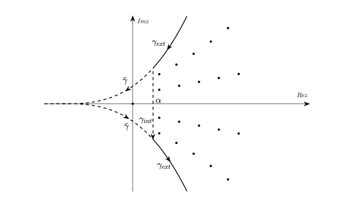
Figure 1: Sketch of the cusp-shaped region of the complex plane enclosing the spectrum of $\mathcal{K}$ and $\mathcal{Q}\mathcal{K}\mathcal{Q}$. The curve $\gamma_{ext}$ represents the boundary of the cusp. We denote by $\partial\mathcal{S}_{\mathcal{K}}$ the curve defined by the union of $\gamma_{ext}$ and $\bar{\gamma}$, while $\partial\mathcal{S}^{\prime}_{\mathcal{K}}$ is defined by the union $\gamma_{ext}$ (up to intersection with $\gamma_{int}$) and $\gamma_{int}$.

One of the key estimates used by Eckmann and Hairer in the proof of Theorem 1 is

$$\frac{1}{4}|z+1|^{2/M}\|u\|^{2}\leq C_{1}\left([1+\operatorname{Re}z]^{2}\|u\|^{2}+\|(\mathcal{K}-z)u\|^{2}\right),\qquad\forall\operatorname{Re}z\geq 0.$$ (29)

In a series of papers, Hèrau, Nier and Helffer [21, 20] proved that the Kolmogorov operator $\mathcal{K}$ corresponding to classical Langevin dynamics generates a semigroup $e^{-t\mathcal{K}}$ that decays exponentially fast to an equilibrium state. Hereafter we show that similar results can be obtained for Kolmogorov operators in the more general form (22).

Theorem 2.

Suppose that $\mathcal{K}$ satisfies all conditions in Theorem 1. If the spectrum $\sigma(\mathcal{K})$ of $\mathcal{K}$ in $L^{2}(\mathbb{R}^{n})$ is such that

$$\sigma(\mathcal{K})\cap i\mathbb{R}=\{0\},$$ (30)

then for any $0<\alpha<\min(\operatorname{Re}\sigma(\mathcal{K})/\{0\})$, there exits a positive constant $C=C(\alpha)$ such that the estimate

$$\|e^{-t\mathcal{K}}u_{0}-\pi_{0}u_{0}\|\leq Ce^{-\alpha t}\|u_{0}\|$$ (31)

holds for all $u_{0}\in L^{2}(\mathbb{R}^{n})$ and for all $t>0$, where $\pi_{0}$ is the spectral projection onto the kernel of $\mathcal{K}$.

Proof.

The Kolmogorov operator $\mathcal{K}$ is closed, maximal-accretive and densely defined in $L^{2}(\mathbb{R}^{n})$. Hence, by the Lumer-Phillips theorem, the semigroup $e^{-t\mathcal{K}}$ is a contraction in $L^{2}(\mathbb{R}^{n})$. It was shown in [13, 21] that the core of $\mathcal{K}$ is the Schwartz space, and that the hypoelliptic estimate (29) holds for any $u\in L^{2}(\mathbb{R}^{n})$. According to Theorem 1, $\mathcal{K}$ only has a discrete spectrum, i.e., $\sigma(\mathcal{K})=\sigma_{dis}(\mathcal{K})$. Condition (30) requires that $\lambda=0$ is the only eigenvalue on the immaginary axis $i\mathbb{R}$. This condition, together with the von-Neumann theorem (see the proof of Theorem 6.1 in [20]), allows us to obtain a weakly convergent Dunford integral [37] representation of the semigroup $e^{-t\mathcal{K}}$ given by

$$e^{-t\mathcal{K}}u_{0}-\pi_{0}u_{0}=\frac{1}{2\pi i}\int_{\partial\mathcal{S}^{\prime}_{\mathcal{K}}}e^{-tz}(z-\mathcal{K})^{-1}u_{0}dz,$$ (32)

where $\partial\mathcal{S}^{\prime}_{\mathcal{K}}=\gamma_{int}\,\cup\,\gamma_{ext}$ is the union of the two curves shown in Figure 1, and $(z-\mathcal{K})^{-1}$ is the resolvent of $\mathcal{K}$. Weak convergence is relative to the inner product

$$\langle(e^{-t\mathcal{K}}-\pi_{0})u_{0},\phi\rangle=\frac{1}{2\pi i}\int_{\partial\mathcal{S}^{\prime}_{\mathcal{K}}}\langle e^{-tz}(z-\mathcal{K})^{-1}u_{0},\phi\rangle dz$$ (33)

for $u_{0}\in L^{2}(\mathbb{R}^{n})$ and $\phi\in D(\mathcal{K}^{*})$. Equation (32) allows us to formulate the semigroup estimation problem as an estimation problem involving an integral in the complex plane. In particular, to derive the upper bound (31), we just need an upper bound for the norm of resolvent $(z-\mathcal{K})^{-1}$. To derive such bound, we notice that for all $z\not\in\mathcal{S}_{\mathcal{K}}$, where $\mathcal{S}_{\mathcal{K}}$ is the cusp (28), and $\operatorname{Re}z\geq 0$, we have $|z+1|^{2/M}\geq(8C_{1})(1+\operatorname{Re}z)^{2}$. A substitution of this inequality into (29) yields, for all $u\in L^{2}(\mathbb{R}^{n})$

$$\frac{1}{8}|z+1|^{2/M}\|u\|^{2} \leq C_{1}\|(\mathcal{K}-z)u\|^{2},\qquad\forall\operatorname{Re}z\geq 0,z\not\in\mathcal{S}_{\mathcal{K}}.$$

Hence, $\|(\mathcal{K}-z)^{-1}\|\leq\sqrt{8C_{1}}|z+1|^{-1/M}$. Next, we rewrite the Dunford integral (32) as

$$\frac{1}{2\pi i}\int_{\partial\mathcal{S}^{\prime}_{\mathcal{K}}}e^{-tz}(z-\mathcal{K})^{-1}u_{0}dz=\frac{1}{2\pi i}\int_{\gamma_{int}}e^{-tz}(z-\mathcal{K})^{-1}u_{0}dz+\frac{1}{2\pi i}\int_{\gamma_{ext}}e^{-tz}(z-\mathcal{K})^{-1}u_{0}dz.$$ (34)

Since $(\mathcal{K}-z)^{-1}$ is a compact linear operator, we have that for any $0<\alpha<\min(\operatorname{Re}\sigma(\mathcal{K})/\{0\})$ there exits a constant $C_{\alpha}>0$ such that $\|(\mathcal{K}-\alpha)u\|\geq C_{\alpha}\|u\|$. On the other hand, $\mathcal{K}$ is also a real operator, which implies that for all complex numbers $z=(\alpha+iy)\not\in\sigma(\mathcal{K})$, we have

$$\|(\mathcal{K}-(\alpha+iy))u\|^{2} =\|(\mathcal{K}-\alpha)u\|^{2}+y^{2}\|u\|^{2}\geq(C_{\alpha}^{2}+y^{2})\|u\|^{2},$$

i.e.,

$$\|(\mathcal{K}-(\alpha+iy))^{-1}u\| \leq\frac{1}{\sqrt{C_{\alpha}^{2}+y^{2}}}\|u\|.$$ (35)

This suggests that the resolvent $(\mathcal{K}-z)^{-1}$ is uniformly bounded by $1/C_{\alpha}$ along the line $\gamma_{int}$, which leads to

$$\left\|\frac{1}{2\pi i}\int_{\gamma_{int}}e^{-tz}(z-\mathcal{K})^{-1}u_{0}dz\right\|\leq Ce^{-\alpha t}\|u_{0}\|.$$ (36)

The boundary $\gamma_{ext}$ is defined by all complex numbers $z=x+iy$ such that $|z+1|=(8C_{1})^{M/2}(1+\operatorname{Re}z)^{M}$. Also, if $z\not\in\mathcal{S}_{\mathcal{K}}$ then the norm of the resolvent is bounded by $\|(\mathcal{K}-z)^{-1}\|\leq\sqrt{8C_{1}}|z+1|^{-1/M}=(x+1)^{-1}$. Combining these two inequalities yields

$$\left\|\frac{1}{2\pi i}\int_{\gamma_{ext}}e^{-tz}(z-\mathcal{K})^{-1}u_{0}dz\right\| \leq C\|u_{0}\|\int_{\gamma_{ext}}^{\infty}e^{-tx}(1+x)^{-1}dz$$

$$\leq C\|u_{0}\|\int_{\alpha}^{\infty}e^{-tx}dx\leq C\|u_{0}\|\frac{e^{-\alpha t}}{t}\qquad t>0.$$ (37)

At this point we recall that $e^{-t\mathcal{K}}$ is a dissipative semigroup and that $\pi_{0}$ is a projection operator into the kernel of $\mathcal{K}$. This allows us to write $\|e^{-t\mathcal{K}}u_{0}-\pi_{0}u_{0}\|=\|e^{-t\mathcal{K}}(u_{0}-\pi_{0}u_{0})\|\leq\|u_{0}-\pi_{0}u_{0}\|$. By combining this inequality with (32), (34), (36) and (3.1) we see that there exists a constant $C=C(\alpha)$ such that

$$\|e^{-t\mathcal{K}}u_{0}-\pi_{0}u_{0}\|\leq Ce^{-\alpha t}\|u_{0}\|.$$ (38)

This completes the proof.

∎

In the following Corollary we derive an upper bound for the norm of the derivatives of the semigroup $e^{-t\mathcal{K}}$.

Corollary 2.1.

Suppose that $\mathcal{K}$ satisfies all conditions listed in Theorem 2. Then for any $t>0$, the $n$-th order time derivative of the semigroup $e^{-t\mathcal{K}}$ satisfies

$$\|e^{-t\mathcal{K}}\mathcal{K}^{n}u_{0}\|\leq\left(\|\pi_{0}\mathcal{K}\|+B\left(\frac{t}{n}\right)\right)^{n}\|u_{0}\|,$$ (39)

where

$$B(t)=Ce^{-\alpha t}\left[1+\frac{1}{t}+\frac{1}{t^{2}}+\cdots\frac{1}{t^{M}}\right],$$ (40)

$C$ is a positive constant, $\alpha$ and $\pi_{0}$ are defined in Theorem 2, and $M$ is the constant defining the cusp (28).

Proof.

By combining the resolvent identity $(z-\mathcal{K})^{-1}\mathcal{K}=z(z-\mathcal{K})^{-1}-\mathcal{I}$ with the Cauchy integral representation theorem and the Dunford integral representation (32) we obtain, for all $t>0$,

$$e^{-t\mathcal{K}}\mathcal{K}-\pi_{0}\mathcal{K} =\frac{1}{2\pi i}\int_{\partial\mathcal{S}^{\prime}_{\mathcal{K}}}e^{-tz}(z-\mathcal{K})^{-1}\mathcal{K}dz$$

$$=\frac{1}{2\pi i}\int_{\partial\mathcal{S}^{\prime}_{\mathcal{K}}}ze^{-tz}(z-\mathcal{K})^{-1}dz.$$ (41)

As before, we split the integral along $\partial\mathcal{S}^{\prime}_{\mathcal{K}}$ into the sum of two integrals (see equation (34))

$$e^{-t\mathcal{K}}\mathcal{K}-\pi_{0}\mathcal{K}=\frac{1}{2\pi i}\left(\int_{\gamma_{int}}ze^{-tz}(z-\mathcal{K})^{-1}dz+\int_{\gamma_{ext}}ze^{-tz}(z-\mathcal{K})^{-1}dz\right).$$ (42)

If $z=x+iy$ is in $\gamma_{int}$ then we have that $|z|$ is bounded by constant. By using the uniform boundedness of the resolvent (35) we obtain

$$\left\|\frac{1}{2\pi i}\int_{\gamma_{int}}e^{-tz}z(z-\mathcal{K})^{-1}dz\right\|\leq Ce^{-\alpha t}.$$ (43)

To derive an upper bound for the second integral in (42), we notice that if $z=x+iy$ is in $\gamma_{ext}$, then $|z|<|z+1|=(8C_{1})^{M/2}(1+x)^{M}$ and $\|(z-\mathcal{K})^{-1}\|\leq\sqrt{8C_{1}}|z+1|^{-1/M}=(1+x)^{-1}$. A substitution of these estimates into the second integral at the right hand side of (42) yields, for all $t>0$,

$$\left\|\frac{1}{2\pi i}\int_{\gamma_{ext}}ze^{-tz}(z-\mathcal{K})^{-1}dz\right\| \leq C\int_{\alpha}^{\infty}e^{-tx}(1+x)^{M-1}dx$$

$$\leq Ce^{-\alpha t}\left[\frac{1}{t}+\frac{1}{t^{2}}+\cdots\frac{1}{t^{M}}\right]$$

$$\leq\underbrace{Ce^{-\alpha t}\left[1+\frac{1}{t}+\frac{1}{t^{2}}+\cdots\frac{1}{t^{M}}\right]}_{B(t)}.$$ (44)

Combining (43) and (3.1) we conclude that the Dunford integral (41) is bounded by $B(t)$. Since $\mathcal{K}$ has a compact resolvent, if there is any zero eigenvallue then it must have finite algebraic multiplicity (Theorem 6.29, Page 187 in [24]). This implies that the projection operator $\pi_{0}$ is a finite rank operator that admits the canonical form (in $L^{2}$)

$$\pi_{0}=\sum_{i=1}^{n}\alpha_{i}\langle\cdot,v_{i}\rangle u_{i}.$$ (45)

On the other hand, since

$$\pi_{0}\mathcal{K}f= \sum_{i=1}^{n}\alpha_{i}\langle\mathcal{K}f,v_{i}\rangle u_{i}$$

$$= \sum_{i=1}^{n}\alpha_{i}\langle f,\mathcal{K}^{*}v_{i}\rangle u_{i},$$

where $\mathcal{K}^{*}$ is the $L^{2}$-adjoint of $\mathcal{K}$, we have

$$\|\pi_{0}\mathcal{K}\|\leq\sum_{i=1}^{n}|\alpha_{i}|\|\mathcal{K}^{*}v_{i}\|\|u_{i}\|.$$ (46)

Hence, $\pi_{0}\mathcal{K}$ is a bounded operator. By using the Dunford integral representation over $\partial\mathcal{S}_{\mathcal{K}}$ it is straightforward to show that $e^{-t\mathcal{K}}\mathcal{K}$ is also a bounded operator for $t>0$. Combining these results with the triangle inequality, we have that for any fixed $t>0$ and any $n\in\mathbb{N}$

$$\left|\left\|e^{-t\mathcal{K}/n}\mathcal{K}\right\|-\left\|\pi_{0}\mathcal{K}\right\|\right|\leq\left\|e^{-t\mathcal{K}/n}\mathcal{K}-\pi_{0}\mathcal{K}\right\|\leq B\left(\frac{t}{n}\right).$$ (47)

Finally, by using the operator identity $e^{-t\mathcal{K}}\mathcal{K}^{n}=(e^{-t\mathcal{K}/n}\mathcal{K})^{n}$ we obtain

$$\left\|e^{-t\mathcal{K}}\mathcal{K}^{n}\right\|\leq\left\|e^{-t\mathcal{K}/n}\mathcal{K}\right\|^{n}\leq\left(B\left(\frac{t}{n}\right)+\left\|\pi_{0}\mathcal{K}\right\|\right)^{n}\qquad t>0,$$ (48)

which completes the proof.

∎

The inequality (39) suggests the flow defined by the semigroup $e^{-t\mathcal{K}}$ has bounded derivatives in time. We emphasize that the estimate (39) is not sufficent to prove the convergence of the formal power series expansion of $e^{-t\mathcal{K}}$ since

$$\lim_{n\rightarrow\infty}\frac{\|e^{-t\mathcal{K}}\mathcal{K}^{n}\|}{n!}\neq 0.$$ (49)

3.2 Analysis of the projected Kolmogorov operator

In this section we analyze the semigroup $e^{-t\mathcal{Q}\mathcal{K}\mathcal{Q}}$ generated by the operator $\mathcal{Q}\mathcal{K}\mathcal{Q}$, where $\mathcal{K}$ is the Kolmogorov operator (4), $\mathcal{P}$ and $\mathcal{Q}=\mathcal{I}-\mathcal{P}$ are projection operators in $L^{2}(\mathbb{R}^{n})$. Such semigroup appears in the EMZ memory and fluctuation terms (see Eqs. (10), (12c) and (12d)). In principle, the projection operator $\mathcal{P}$ and therefore the complementary projection $\mathcal{Q}$ can be chosen arbitrarily [53, 6]. Here we restrict our analysis to finite-rank symmetric projections in $L^{2}(\mathbb{R}^{n})$. Mori’s projection (9) is one of such projections.

Theorem 3.

Let $\mathcal{P}:L^{2}(\mathbb{R}^{n})\rightarrow L^{2}(\mathbb{R}^{n})$ be a finite-rank, symmetric projection operator. If $\mathcal{K}$ satisfies all conditions listed in Theorem 1, then the operator $\mathcal{Q}\mathcal{K}\mathcal{Q}$ is also maximal accretive and has a compact resolvent. Moreover, the spectrum of $\mathcal{Q}\mathcal{K}\mathcal{Q}$ lies within the cusp

$$\mathcal{S}_{\mathcal{Q}\mathcal{K}\mathcal{Q}}=\{z\in\mathbb{C}|\operatorname{Re}z\geq 0,|z+1|<(8C_{\mathcal{Q}})^{M_{\mathcal{Q}}/2}(1+\operatorname{Re}z)^{M_{\mathcal{Q}}}\}$$ (50)

for some the positive constants $C_{\mathcal{Q}}$ and integer $M_{\mathcal{Q}}$.

Proof.

We first show that if $\mathcal{K}$ is closely defined and maximal accretive, and that $\mathcal{Q}\mathcal{K}\mathcal{Q}$ has the same properties. According to the Lumer-Phillips theorem [15], the adjoint of a maximal-accretive operator is accretive, and therefore

$$\operatorname{Re}\langle\mathcal{K}f,f\rangle \geq 0\qquad\forall f\in D(\mathcal{K}),$$

$$\operatorname{Re}\langle\mathcal{K}^{*}f,f\rangle \geq 0\qquad\forall f\in D(\mathcal{K}^{*}).$$

Here $D(\mathcal{K})$ and $D(\mathcal{K}^{*})$ denote the domain of the linear operators $\mathcal{K}$ and $\mathcal{K}^{*}$, respectively (see, e.g., [45]). On the other hand, if $\mathcal{P}$ is a symmetric operator in $L^{2}(\mathbb{R}^{n})$ then $\mathcal{Q}=\mathcal{I}-\mathcal{P}$ is also symmetric. This implies that

$$\operatorname{Re}\langle\mathcal{Q}\mathcal{K}\mathcal{Q}f,f\rangle =\operatorname{Re}\langle\mathcal{K}\mathcal{Q}f,\mathcal{Q}f\rangle\geq 0\qquad\forall f\in D(\mathcal{K}),$$

$$\operatorname{Re}\langle(\mathcal{Q}\mathcal{K}\mathcal{Q})^{*}f,f\rangle =\operatorname{Re}\langle\mathcal{K}^{*}\mathcal{Q}f,\mathcal{Q}f\rangle\geq 0\qquad\forall f\in D(\mathcal{K}^{*}),$$

i.e., $\mathcal{Q}\mathcal{K}\mathcal{Q}$ and its adjoint $\mathcal{Q}\mathcal{K}^{*}\mathcal{Q}$ are both maximal-accretive. $\mathcal{Q}\mathcal{K}\mathcal{Q}$ is also a closable operator defined in $D(\mathcal{K})$. This can be seen by decomposing it as $\mathcal{Q}\mathcal{K}\mathcal{Q}=\mathcal{K}-\mathcal{K}\mathcal{P}-\mathcal{P}\mathcal{K}\mathcal{Q}$. In fact, if $\mathcal{K}$ is a closed operator then $\mathcal{Q}\mathcal{K}\mathcal{Q}$ is closed since $\mathcal{K}\mathcal{P}$ and $\mathcal{P}\mathcal{K}\mathcal{Q}$ are bounded [24], as we shall see hereafter. By using the Lumer-Philips theorem, we conclude that $\mathcal{Q}\mathcal{K}\mathcal{Q}$ is also maximal accretive, and its closure generates a contraction semigroup $e^{-t\mathcal{Q}\mathcal{K}\mathcal{Q}}$ in $L^{2}(\mathbb{R}^{n})$. Next, we show that if $\mathcal{K}$ satisfies the hypoelliptic estimate $\|u\|_{\delta,\delta}\leq C(\|u\|+\|\mathcal{K}u\|)$, then so does $\mathcal{Q}\mathcal{K}\mathcal{Q}$, i.e.,

$$\|u\|_{\delta,\delta}\leq C(\|u\|+\|\mathcal{Q}\mathcal{K}\mathcal{Q}u\|).$$ (51)

By using triangle inequality we obtain

$$\|u\|_{\delta,\delta}\leq C(\|u\|+\|\mathcal{K}u\|)\leq C(\|u\|+\|\mathcal{K}\mathcal{P}u\|+\|\mathcal{Q}\mathcal{K}\mathcal{Q}u\|+\|\mathcal{P}\mathcal{K}\mathcal{Q}u\|).$$

To prove (51), it is sufficient to show that $\mathcal{K}\mathcal{P}$ and $\mathcal{P}\mathcal{K}\mathcal{Q}$ are bounded operators in $L^{2}(\mathbb{R}^{n})$. To this end, we recall that any finite-rank projection admits the canonical representation

$$\mathcal{P}=\sum_{i=1}^{m}\lambda_{i}\langle\cdot,\phi_{i}\rangle\varphi_{i},$$ (52)

where $\{\phi_{i}\}_{i=1}^{m}$ and $\{\varphi_{i}\}_{i=1}^{m}$ are elements $L^{2}(\mathbb{R}^{n})$. This implies that

$$\|\mathcal{K}\mathcal{P}u\| =\left\|\sum_{i=1}^{m}\lambda_{i}\langle u,\phi_{i}\rangle\mathcal{K}\varphi_{i}\right\|\leq\sum_{i=1}^{m}|\lambda_{i}|\|\mathcal{K}\varphi_{i}\|\|\phi_{i}\|\|u\|=C\|u\|,$$ (53)

$$\|\mathcal{P}\mathcal{K}\mathcal{Q}u\| =\left\|\sum_{i=1}^{m}\lambda_{i}\langle\mathcal{K}\mathcal{Q}u,\phi_{i}\rangle\varphi_{i}\right\|=\left\|\sum_{i=1}^{m}\lambda_{i}\langle u,\mathcal{Q}\mathcal{K}^{*}\phi_{i}\rangle\varphi_{i}\right\|\leq\sum_{i=1}^{m}|\lambda_{i}|\|\mathcal{Q}\mathcal{K}^{*}\phi_{i}\|\|\varphi_{i}\|\|u\|=C\|u\|.$$ (54)

This proves that $\mathcal{K}\mathcal{P}$ and $\mathcal{P}\mathcal{K}\mathcal{Q}$ are both bounded linear operators. At this point we notice that if $\mathcal{Q}\mathcal{K}\mathcal{Q}$ is accretive, then $(\mathcal{Q}\mathcal{K}\mathcal{Q}+\mathcal{I})$ invertible. Moreover, since $\mathcal{K}$ is accretive we have

$$\|(\mathcal{Q}\mathcal{K}\mathcal{Q}+\mathcal{I})u\|^{2}=\|\mathcal{Q}\mathcal{K}\mathcal{Q}\|^{2}+2\operatorname{Re}\langle\mathcal{K}\mathcal{Q}u,\mathcal{Q}u\rangle+\|u\|^{2}\geq\|\mathcal{Q}\mathcal{K}\mathcal{Q}\|^{2}+\|u\|^{2}.$$

This implies that

$$\|u\|_{\delta,\delta}\leq C(\|u\|+\|\mathcal{Q}\mathcal{K}\mathcal{Q}u\|)\leq\sqrt{2}C\|(\mathcal{Q}\mathcal{K}\mathcal{Q}+\mathcal{I})u\|\Rightarrow\|(\mathcal{Q}\mathcal{K}\mathcal{Q}+\mathcal{I})^{-1}u\|_{\delta,\delta}\leq\sqrt{2}C\|u\|,$$

i.e., $(\mathcal{Q}\mathcal{K}\mathcal{Q}+\mathcal{I})^{-1}$ is a bounded operator from $L^{2}$ into the weighted Sobolev space $\mathcal{S}^{\delta,\delta}$ defined in (24). At this point we recall that $S^{\delta,\delta}$ is compactly embedded into $L^{2}$ (Lemma 3.2 [13]). Hence, $(\mathcal{Q}\mathcal{K}\mathcal{Q}+\mathcal{I})^{-1}$ is compact from $L^{2}$ into $L^{2}$ and therefore $\mathcal{Q}\mathcal{K}\mathcal{Q}$ has a compact resolvent [24]. To prove that the discrete spectrum of $\mathcal{Q}\mathcal{K}\mathcal{Q}$ lies within the cusp $\mathcal{S}_{\mathcal{Q}\mathcal{K}\mathcal{Q}}$ defined in (50), we follow the procedure outlined in [13]. To this end, let $\mathcal{K}\in\text{Pol}_{2}^{N}$. Then, for $\delta=\max\{2,N\}$ we have the bound

$$\|(\mathcal{K}+\mathcal{I})u\|\leq C\|u\|_{\delta,\delta}\qquad\forall u\in\mathscr{S}_{n},$$

and

$$\|(\mathcal{Q}\mathcal{K}\mathcal{Q}+\mathcal{I})u\|\leq\|\mathcal{Q}\|(\|\mathcal{K}u\|+\|\mathcal{K}\mathcal{P}u\|)+\|u\|\leq C(\|\mathcal{K}u\|+\|u\|)\leq\sqrt{2}C\|(\mathcal{K}+\mathcal{I})u\|\leq C\|u\|_{\delta,\delta}.$$

Recall that $\mathcal{Q}\mathcal{K}\mathcal{Q}:D(\mathcal{Q}\mathcal{K}\mathcal{Q})\rightarrow L^{2}(\mathbb{R}^{2d})$ is maximally accretive. Therefore, by Lemma 4.5 in [13], for all $\delta>0$ we can find an integer $M_{\mathcal{Q}}>0$ and a constant $C$ such that

$$\langle u,[(\mathcal{Q}\mathcal{K}\mathcal{Q}+\mathcal{I})^{*}(\mathcal{Q}\mathcal{K}\mathcal{Q}+\mathcal{I})]^{1/M_{\mathcal{Q}}}\rangle\leq C\|u\|^{2}_{\delta,\delta}.$$ (55)

By using the hypoelliptic estimate (55), (51), Proposition B.1 in [20] and the triangle inequality we obtain

$$\frac{1}{4}|z+1|^{2/M_{\mathcal{Q}}}\|u\|^{2} \leq C\|u\|^{2}_{\delta,\delta}+\|(\mathcal{Q}\mathcal{K}\mathcal{Q}-z)\|^{2}$$

$$\leq C_{\mathcal{Q}}([1+\operatorname{Re}z]^{2}\|u\|^{2}+\|(\mathcal{Q}\mathcal{K}\mathcal{Q}-z)u\|^{2}).$$

This result, together with the compactness of the resolvent of $\mathcal{Q}\mathcal{K}\mathcal{Q}$, implies that if $z\in\sigma(\mathcal{Q}\mathcal{K}\mathcal{Q})$ (spectrum of $\mathcal{Q}\mathcal{K}\mathcal{Q}$) then

$$\frac{1}{8}|z+1|^{2/M_{\mathcal{Q}}}\|u\|^{2}<\frac{1}{4}|z+1|^{2/M_{\mathcal{Q}}}\|u\|^{2}\leq C_{\mathcal{Q}}(1+\operatorname{Re}z)^{2}\|u\|^{2}.$$

This proves that the spectrum of $\mathcal{Q}\mathcal{K}\mathcal{Q}$ is contained in the cusp-shaped region $\mathcal{S}_{\mathcal{Q}\mathcal{K}\mathcal{Q}}$ defined in equation (50). If $z\not\in\mathcal{S}_{\mathcal{Q}\mathcal{K}\mathcal{Q}}$, then we have resolvent estimate

$$\|(\mathcal{Q}\mathcal{K}\mathcal{Q}-z)^{-1}\|\leq\sqrt{8C_{\mathcal{Q}}}|z+1|^{-1/M_{\mathcal{Q}}}.$$ (56)

∎

Remark

The main assumption at the basis of Theorem 3 is that $\mathcal{P}$ is a finite-rank symmetric projection. Mori’s projection (9) is one of such projections. If $\mathcal{P}$ is of finite-rank then both $\mathcal{K}\mathcal{P}$ and $\mathcal{P}\mathcal{K}\mathcal{Q}$ are bounded operators, which yields the hypoelliptic estimate (26). On the other hand, if $\mathcal{P}$ is an infinite-rank projection, e.g., Chorin’s projection [53, 7, 8, 59], then $\mathcal{K}\mathcal{P}$ and $\mathcal{P}\mathcal{K}\mathcal{Q}$ may not be bounded. Whether Theorem 3 holds for infinite-rank projections is an open question.

With the resolvent estimate (56) available, we can now prove the analog of Theorem 2 and Corollary 2.1, with $\mathcal{K}$ replaced by $\mathcal{Q}\mathcal{K}\mathcal{Q}$. These results establish exponential relaxation to equilibrium of $e^{-t\mathcal{Q}\mathcal{K}\mathcal{Q}}$ and the regularity of the EMZ orthogonal dynamics induced by $e^{-t\mathcal{Q}\mathcal{K}\mathcal{Q}}$.

Theorem 4.

Assume that $\mathcal{K}$ satisfies all conditions listed in Theorem 1. Let $\mathcal{P}:L^{2}(\mathbb{R}^{n})\rightarrow L^{2}(\mathbb{R}^{n})$ be a symmetric finite-rank projection operator. If the spectrum of $\mathcal{Q}\mathcal{K}\mathcal{Q}$ in $L^{2}(\mathbb{R}^{n})$ satisfies

$$\sigma(\mathcal{Q}\mathcal{K}\mathcal{Q})\cap i\mathbb{R}\subseteq\{0\},$$ (57)

then for any $0<\alpha_{\mathcal{Q}}<\min(\operatorname{Re}\sigma(\mathcal{Q}\mathcal{K}\mathcal{Q})/\{0\})$ there exits a positive constant $C=C(\alpha_{\mathcal{Q}})$ such that

$$\|e^{-t\mathcal{Q}\mathcal{K}\mathcal{Q}}u_{0}-\pi^{\mathcal{Q}}_{0}u_{0}\|\leq Ce^{-\alpha_{\mathcal{Q}}t}\|u_{0}\|,$$ (58)

for all $u_{0}\in L^{2}(\mathbb{R}^{n})$ and for all $t>0$, where $\pi^{\mathcal{Q}}_{0}$ is the spectral projection onto the kernel of $\mathcal{Q}\mathcal{K}\mathcal{Q}$.

Corollary 4.1.

Suppose that $\mathcal{P}$ and $\mathcal{K}$ satisfy all conditions listed in Theorem 4. Then for any $t>0$ the $n$-th order derivative of the semigroup $e^{-t\mathcal{Q}\mathcal{K}\mathcal{Q}}$ satisfies

$$\|e^{-t\mathcal{Q}\mathcal{K}\mathcal{Q}}(\mathcal{Q}\mathcal{K}\mathcal{Q})^{n}u_{0}\|\leq\left(\|\pi_{0}(\mathcal{Q}\mathcal{K}\mathcal{Q})\|+B_{\mathcal{Q}}\left(\frac{t}{n}\right)\right)^{n}\|u_{0}\|,$$ (59)

where the function $B_{\mathcal{Q}}(t)$ has the same form as (40), with $\alpha$ replaced by $\alpha_{\mathcal{Q}}$ and $M$ replaced by $M_{\mathcal{Q}}$.

The proofs of Theorem 4 and Corollary 4.1 closely follow the proofs of Theorem 2 and Corollary 2.1. Therefore we omit them. The semigroup estimate (58) allows us to prove exponential convergence to the equilibrium state of the EMZ memory kernel and fluctuation force. Specifically, we have the following:

Corollary 4.2.

Consider a scalar observable $u(t)=u(\bm{x}(t))$ with initial condition $u(0)=u_{0}$, and let $\mathcal{P}(\cdot)=\langle(\cdot),u_{0}\rangle u_{0}$ be a one-dimensional Mori’s projection (9). Then the EMZ memory kernel (12c) converges exponentially fast to the equilibrium state $\langle\mathcal{Q}\mathcal{K}^{*}u_{0},\pi^{\mathcal{Q}}_{0}\mathcal{K}u_{0}\rangle$, with rate $\alpha_{\mathcal{Q}}$. In other words, there exists a positive constant $C$ such that

$$|K(t)-\langle\mathcal{Q}\mathcal{K}^{*}u_{0},\pi^{\mathcal{Q}}_{0}\mathcal{K}u_{0}\rangle|\leq Ce^{-\alpha_{\mathcal{Q}}t}.$$ (60)

Proof.

A substitution of (58) into (12c) and subsequent application of Cauchy-Schwartz inequality yields

$$|K(t)-\langle\mathcal{Q}\mathcal{K}^{*}u_{0},\pi^{\mathcal{Q}}_{0}\mathcal{K}u_{0}\rangle| =|\langle u_{0},\mathcal{K}e^{t\mathcal{Q}\mathcal{K}\mathcal{Q}}\mathcal{Q}\mathcal{K}u_{0}\rangle-\langle\mathcal{Q}\mathcal{K}^{*}u_{0},\pi^{\mathcal{Q}}_{0}\mathcal{K}u_{0}\rangle|$$

$$=|\langle\mathcal{Q}\mathcal{K}^{*}u_{0},e^{t\mathcal{Q}\mathcal{K}\mathcal{Q}}\mathcal{K}u_{0}\rangle-\langle\mathcal{Q}\mathcal{K}^{*}u_{0},\pi^{\mathcal{Q}}_{0}\mathcal{K}u_{0}\rangle|$$

$$\leq C\|\mathcal{Q}\mathcal{K}^{*}u_{0}\|\|\mathcal{K}u_{0}\|e^{-\alpha_{\mathcal{Q}}t}.$$ (61)

∎

It is straightforward to generalize Corollary 4.2 to matrix-valued memory kernels (12c) and obtain the following exponential convergence result

$$\|\bm{K}(t)-\bm{G}^{-1}\bm{C}^{\mathcal{Q}}\|_{\mathscr{M}}\leq C\|\bm{G}^{-1}\bm{D}^{\mathcal{Q}}\|_{\mathscr{M}}e^{-\alpha_{\mathcal{Q}}t},$$ (62)

where $\|\cdot\|_{\mathscr{M}}$ denotes any matrix norm and $\bm{G}$ is the Gram matrix (12a). Also, the matrix $\bm{C}^{\mathcal{Q}}$ has entries $C^{\mathcal{Q}}_{ij}=\langle\mathcal{Q}\mathcal{K}^{*}u_{i}(0),\pi^{\mathcal{Q}}_{0}\mathcal{K}u_{j}(0)\rangle$, while $D^{\mathcal{Q}}_{ij}=\|\mathcal{Q}\mathcal{K}u_{i}(0)\|\|\mathcal{K}u_{j}(0)\|$. The proof of (62) follows immediately from the following inequality

$$\langle u_{i}(0),\mathcal{K}e^{t\mathcal{Q}\mathcal{K}\mathcal{Q}}\mathcal{Q}\mathcal{K}u_{j}(0)\rangle-\langle\mathcal{Q}\mathcal{K}^{*}u_{i}(0),\pi^{\mathcal{Q}}_{0}\mathcal{K}u_{j}(0)\rangle =\langle\mathcal{Q}\mathcal{K}^{*}u_{i}(0),e^{t\mathcal{Q}\mathcal{K}\mathcal{Q}}\mathcal{K}u_{j}(0)-\pi^{\mathcal{Q}}_{0}\mathcal{K}u_{j}(0)\rangle$$

$$\leq C\|\mathcal{Q}\mathcal{K}u_{i}(0)\|\|\mathcal{K}u_{j}(0)\|e^{-\alpha_{\mathcal{Q}}t}.$$ (63)

In fact, a substitution of (3.2) into (12c) yields (62). Similarly, we can prove that the fluctuation term (12d) reaches the equilibrium state exponentially fast in time. If we choose the initial condition as $\bm{u}_{0}=\mathcal{Q}\mathcal{K}\bm{u}_{0}$ then for all $j=1,...,m$, we have

$$\|f_{j}(t)-\pi^{\mathcal{Q}}_{0}\mathcal{Q}\mathcal{K}u_{j}(0)\|=\|e^{-t\mathcal{Q}\mathcal{K}\mathcal{Q}}\mathcal{Q}\mathcal{K}u_{j}(0)-\pi^{\mathcal{Q}}_{0}\mathcal{Q}\mathcal{K}u_{j}(0)\|\leq Ce^{-\alpha_{\mathcal{Q}}t}\|\mathcal{Q}\mathcal{K}u_{j}(0)\|.$$ (64)

Let us now introduce the tensor product space $\displaystyle V=\otimes_{i=1}^{m}L^{2}(\mathbb{R}^{n})$ and the following norm

$$\|\bm{r}(t)\|_{V}:=\left\|\left(\|r_{1}(t)\|,\|r_{2}(t)\|,\cdots,\|r_{m}(t)\|\right)\right\|_{\mathscr{M}},$$ (65)

where $\|\cdot\|$ is the standard $L^{2}(\mathbb{R}^{n})$ norm, and $\|\cdot\|_{\mathscr{M}}$ is any matrix norm. Then from (64) it follows that

$$\|\bm{f}(t)-\pi^{\mathcal{Q}}_{0}\mathcal{Q}\mathcal{K}\bm{u}_{0}\|_{V}\leq Ce^{-\alpha_{\mathcal{Q}}t}\|\mathcal{Q}\mathcal{K}\bm{u}(0)\|_{V}.$$ (66)

4 An application to Langevin dynamics

All results we obtained so far can be applied to stochastic differential equations of the form (1), provided the MZ projection operator is of finite-rank. In this section, we study in detail the Langevin dynamics of an interacting particle system widely used in statistical mechanics to model liquids and gasses [27, 38], and show that the EMZ memory kernel (12c) and fluctuation term (12d) decay exponentially fast in time to a unique equilibrium state. Such state is defined by the projector operator $\pi_{0}^{\mathcal{Q}}$ appearing in Theorem 4 and Corollary 4.2. Hereafter we will determine the exact expression of such projector for a system of interacting identical particles modeled by the following SDE in $\mathbb{R}^{2d}$

$$\begin{dcases}\frac{d\bm{q}}{dt}=\frac{1}{\mu}\bm{p},\\ \frac{d\bm{p}}{dt}=-\nabla V(\bm{q})-\frac{\gamma}{\mu}\bm{p}+\sigma\bm{\xi}(t),\end{dcases}$$ (67)

where $\mu$ is the mass of each particle, $V(\bm{q})$ is the interaction potential and $\bm{\xi}(t)$ is a $d$-dimensional Gaussian white noise process modeling physical Brownian motion. The parameters $\sigma$ and $\gamma$ represent, respectively, the amplitude of the fluctuations and the viscous dissipation coefficient. Such parameters are linked by the fluctuation-dissipation relation $\sigma=(2\gamma/\beta)^{1/2}$, where $\beta$ is proportional to the inverse of the thermodynamic temperature. The stochastic dynamical system (67) is widely used in statistical mechanics to model the mesoscopic dynamics of liquids and gases. Letting the mass $\mu$ in (67) go to zero, and setting $\gamma=1$ yields the so-called overdamped Langevin dynamics, i.e., Langevin dynamics where no average acceleration takes place. The (negative) Kolmogorov operator (4) associated with the SDE (67) is given by

$$\mathcal{K}=-\frac{\bm{p}}{\mu}\cdot\nabla_{\bm{q}}+\nabla_{\bm{q}}V(\bm{q})\cdot\nabla_{\bm{p}}+\gamma\left(\frac{\bm{p}}{\mu}\cdot\nabla_{p}-\frac{1}{\beta}\Delta_{p}\right),$$ (68)

where “$\cdot$” denotes the standard dot product. If the interaction potential $V(\bm{q})$ is strictly positive at infinity then the Langevin equation (67) admits an unique invariant Gibbs measure given by

$$\rho_{eq}(\bm{p},\bm{q})=\frac{1}{Z}e^{-\beta H(\bm{p},\bm{q})},$$ (69)

where

$$H(\bm{p},\bm{q})=\frac{\|\bm{p}\|_{2}^{2}}{2\mu}+V(\bm{q}),$$ (70)

is the Hamiltonian and $Z$ is the partition function. At this point we introduce the unitary transformation $\mathcal{U}:L^{2}(\mathbb{R}^{2d})\rightarrow L^{2}(\mathbb{R}^{2d},\rho_{eq})$ defined by

$$(\mathcal{U}g)(\bm{p},\bm{q})=\sqrt{Z}e^{\beta H(\bm{p},\bm{q})/2}g(\bm{p},\bm{q}),$$ (71)

where $L^{2}(\mathbb{R}^{2d};\rho_{eq})$ is a weighted Hilbert space endowed with the inner product

$$\langle h,g\rangle_{\rho_{eq}}=\int h(\bm{p},\bm{q})g(\bm{p},\bm{q})\rho_{eq}(\bm{p},\bm{q})d\bm{p}d\bm{q}.$$ (72)

The linear transformation (71) is an isometric isomorphism between the spaces $L^{2}(\mathbb{R}^{2d})$ and $L^{2}(\mathbb{R}^{2d};\rho_{eq})$. In fact, for any $\tilde{u}\in L^{2}(\mathbb{R}^{2d})$, there exists a unique $u\in L^{2}(\mathbb{R}^{2d};\rho_{eq})$ such that $\tilde{u}=(e^{-\beta H/2}/\sqrt{Z})u$ and

$$\|\tilde{u}\|_{L^{2}}=\|u\|_{L^{2}_{eq}}.$$ (73)

By applying (71) to (68) we construct the transformed Kolmogorov operator $\tilde{\mathcal{K}}=\mathcal{U}^{-1}\mathcal{K}\mathcal{U}$, which has the explicit expression

$$\tilde{\mathcal{K}}=-\frac{\bm{p}}{\mu}\cdot\nabla_{\bm{q}}+\nabla V(\bm{q})\cdot\nabla_{\bm{p}}+\frac{\gamma}{\beta}\left(-\nabla_{\bm{p}}+\frac{\beta}{2\mu}\bm{p}\right)\cdot\left(\nabla_{\bm{p}}+\frac{\beta}{2\mu}\bm{p}\right).$$ (74)

This operator can be written in the canonical form (22) as

$$\tilde{\mathcal{K}}=\sum_{i=1}^{d}\mathcal{X}_{i}^{*}\mathcal{X}_{i}-\mathcal{X}_{0},$$ (75)

provided we set

$$\begin{dcases}\mathcal{X}_{0}=\frac{\bm{p}}{\mu}\cdot\nabla_{\bm{q}}-\nabla V(\bm{q})\cdot\nabla_{\bm{p}},\\ \mathcal{X}_{i}=\sqrt{\frac{\gamma}{\beta}}\left(\partial_{p_{i}}+\frac{\beta}{2\mu}p_{i}\right),\\ \mathcal{X}_{i}^{*}=\sqrt{\frac{\gamma}{\beta}}\left(-\partial_{p_{i}}+\frac{\beta}{2\mu}p_{i}\right).\end{dcases}$$ (76)

Note that $\mathcal{X}_{0}$ is skew-symmetric in $L^{2}(\mathbb{R}^{2d})$. Also, $\mathcal{X}_{i}^{*}$ and $\mathcal{X}_{i}$ can be interpreted as creation and annihilation operators, similarly to a harmonic quantum oscillator [57]. The Kolmogorov operator $\tilde{\mathcal{K}}$ and its formal adjoint $\tilde{\mathcal{K}}^{*}$ are both accretive, closable and with maximally accretive closure in $L^{2}(\mathbb{R}^{2d})$ (see, e.g., [21, 20, 12]) Similar to the Kolmogorov operator $\tilde{\mathcal{K}}=\mathcal{U}^{-1}\mathcal{K}\mathcal{U}$, we can transform the MZ projection operators $\mathcal{P}$ and $\mathcal{Q}$ into operators in the “flat” Hilbert space $L^{2}(\mathbb{R}^{2d})$ as $\tilde{\mathcal{P}}=\mathcal{U}^{-1}\mathcal{P}\mathcal{U}$ and $\tilde{\mathcal{Q}}=\mathcal{U}^{-1}\mathcal{Q}\mathcal{U}$. The relationship between $L^{2}(\mathbb{R}^{2d})$, $L^{2}(\mathbb{R}^{2d};\rho_{eq})$ and the operators defined between such spaces can be summarized by the following commutative diagram

The properties of all operators in $L^{2}(\mathbb{R}^{2d})$ and $L^{2}(\mathbb{R}^{2d};\rho_{eq})$ are essentially the same since $\mathcal{U}$ is a bijective isometry. For instance if $\mathcal{P}$ is compact and symmetric then $\tilde{\mathcal{P}}$ is also a compact and symmetric operator.

Next, we apply the analytical results we obtained in Section 3.1 and Section 3.2 to the particle system described by the SDE (67). To this end, we just need to verify whether $\tilde{\mathcal{K}}$ is a poly-Hörmander operator, i.e., if the operators $\{\mathcal{X}_{i}\}_{i=0}^{d}$ appearing in (75)-(76) satisfy the poly-Hörmander conditions in Proposition 1 and the estimate in Theorem 1 (see Section 3.1). This can be achieved by imposing additional conditions on the particle interaction potential $V(\bm{q})$ (see [12, Proposition 3.7]). In particular, following Helffer and Nier [20], we assume that $V(\bm{q})$ satisfies the following weak ellipticity hypothesis

Hypothesis 1.

The particle interaction potential $V(\bm{q})$ is of class $C^{\infty}(\mathbb{R}^{d})$, and for all $\bm{q}\in\mathbb{R}^{d}$ it satisfies the following conditions:

1. $\forall\bm{\alpha}\in\mathbb{N}^{d}$ such that $|\bm{\alpha}|=1$, $|\partial_{\bm{q}}^{\bm{\alpha}}V(\bm{q})|\leq C_{\bm{\alpha}}\sqrt{1+\|\nabla V(\bm{q})\|^{2}}$ for some positive constant $C_{\bm{\alpha}}$,

2. There exists $M\in\mathbb{N}$, and $C\geq 1$, such that $C^{-1}(1+\|\bm{q}\|^{2})^{1/(2M)}\leq\sqrt{1+\|\nabla V(\bm{q})\|^{2}}\leq C(1+\|\bm{q}\|^{2})^{M/2}$.

Hypothesis 1 holds for any particle interaction potential that grows at most polynomially at infinity, i.e., $V(\bm{q})\simeq\|\bm{q}\|^{M}$ as $\left\|\bm{q}\right\|\rightarrow\infty$. With this hypothesis, it is possible to prove the following

Proposition 2 (Helffer and Nier [20]).

Consider the Langevin equation (67) with particle interaction potential $V(\bm{q})$ satisfying Hypothesis 1. Then the operator $\tilde{\mathcal{K}}$ defined in (74) has a compact resolvent, and a discrete spectrum bounded by the cusp $\mathcal{S}_{\mathcal{K}}$. Moreover, there exists a positive constant $C$ such that the estimate

$$\|e^{-t\tilde{\mathcal{K}}}u_{0}-\tilde{\pi}_{0}\tilde{u}_{0}\|\leq Ce^{-\alpha t}\|\tilde{u}_{0}\|$$ (77)

holds for all $\tilde{u}_{0}\in L^{2}(\mathbb{R}^{2d})$ and for all $t>0$, where $\tilde{\pi}_{0}$ is the orthogonal projection onto the kernel of $\tilde{\mathcal{K}}$ in $L^{2}(\mathbb{R}^{2d})$.

By using the isomorphism (71) we can rewrite Proposition 2 in $L^{2}(\mathbb{R}^{2d};\rho_{eq})$ as

$$\|e^{-t\mathcal{K}}u_{0}-\pi_{0}u_{0}\|_{L^{2}_{eq}}=\|e^{-t\tilde{\mathcal{K}}}\tilde{u}_{0}-\tilde{\pi}_{0}\tilde{u}_{0}\|_{L^{2}}\leq Ce^{-\alpha t}\|\tilde{u}_{0}\|_{L^{2}}=Ce^{-\alpha t}\|u_{0}\|_{L^{2}_{eq}},$$ (78)

where $\pi_{0}=\mathcal{U}\tilde{\pi}_{0}\mathcal{U}^{-1}$ is the orthogonal projection $\pi_{0}(\cdot)=\mathbb{E}[(\cdot)]$. The inequality (78) is completely equivalent to the estimate (31). It is also possible to obtain a prior estimate on the convergence rate $\alpha$ by building a connection between the Kolmogorov operator and the Witten Laplacian (see [21, 20] for further details).

Our next task is to derive an estimate for the operator $\tilde{\mathcal{Q}}\tilde{\mathcal{K}}\tilde{\mathcal{Q}}$, and for the semigroup $e^{-t\tilde{\mathcal{Q}}\tilde{\mathcal{K}}\tilde{\mathcal{Q}}}$ generated by the closure of $\tilde{\mathcal{Q}}\tilde{\mathcal{K}}\tilde{\mathcal{Q}}$. According to Theorem 3 the spectrum of $\tilde{\mathcal{Q}}\tilde{\mathcal{K}}\tilde{\mathcal{Q}}$ is bounded by the cusp $\mathcal{S}_{\tilde{\mathcal{Q}}\tilde{\mathcal{K}}\tilde{\mathcal{Q}}}$, provided that $\mathcal{P}$ is an orthogonal finite-rank projection operator. On the other hand, Theorem 4 establishes exponential convergence of $e^{-t\tilde{\mathcal{Q}}\tilde{\mathcal{K}}\tilde{\mathcal{Q}}}$ to equilibrium if $\tilde{\mathcal{Q}}\tilde{\mathcal{K}}\tilde{\mathcal{Q}}$ satisfies condition (57). It is left to determine the exact form of the spectral projection $\tilde{\pi}_{0}^{\tilde{\mathcal{Q}}}$, i.e., the projection onto the kernel of $\tilde{\mathcal{Q}}\tilde{\mathcal{K}}\tilde{\mathcal{Q}}$ (see Theorem 4) and verify condition (57). To this end, we consider a general Mori-type projection $\mathcal{P}$ and its unitarily equivalent version $\tilde{\mathcal{P}}=\mathcal{U}^{-1}\mathcal{P}\mathcal{U}$

$$\mathcal{P}(\cdot)=\sum_{i=1}^{m}\langle\cdot,v_{i}\rangle_{\rho_{eq}}v_{i},\qquad\tilde{\mathcal{P}}(\cdot)=\sum_{i=1}^{m}\langle\cdot,v_{i}\rangle_{\rho_{eq}/2}v_{i}e^{-\beta H/2},$$ (79)

where $\{v_{j}\}_{j=1}^{m}=\{v_{j}(\bm{q},\bm{p})\}_{j=1}^{m}$ are zero-mean, i.e. $\langle v_{i}\rangle_{\rho_{eq}}=0$, orthonormal basis functions. In (79) we used the shorthand notation

$$\langle h\rangle_{\rho_{eq}/2}=\frac{1}{Z}\int g(\bm{p},\bm{q})e^{-\beta H(\bm{p},\bm{q})/2}d\bm{p}d\bm{q}.$$ (80)

Lemma 5.

Suppose that the particle interaction potential $V(\bm{q})$ in (68) satisfies Hypothesis 1. Then for any set of observables $\{w_{j}\}_{j=1}^{m}$ satisfying $\langle w_{j},v_{i}\rangle_{\rho_{eq}}=0$ and $\mathcal{K}w_{j}=v_{j}$ we have that the kernel of $\tilde{\mathcal{Q}}\tilde{\mathcal{K}}\tilde{\mathcal{Q}}$ is given by

$$\textrm{Ker}(\tilde{\mathcal{Q}}\tilde{\mathcal{K}}\tilde{\mathcal{Q}}) =\text{Ker}(\tilde{\mathcal{K}})\,\cup\,\text{Ran}(\tilde{\mathcal{P}})\,\cup\,\text{Span}\{w_{j}e^{-\beta H/2}\}_{j=1}^{m},$$ (81)

where $\tilde{\mathcal{K}}$ and $\tilde{\mathcal{P}}$ are defined in (74) and (79), respectively. In particular, if $\mathcal{P}$ is defined as $\mathcal{P}(\cdot)=\langle\cdot,p_{j}\rangle_{\rho_{eq}}p_{j}$, where $p_{j}$ is the momentum of $j$-th particle, then we have

$$\sigma(\tilde{\mathcal{Q}}\tilde{\mathcal{K}}\tilde{\mathcal{Q}})\cap i\mathbb{R} \subseteq\{0\}.$$ (82)

Proof.

We first prove (81). To this end, let us first define the finite-dimensional space

$$W=\text{Ker}(\tilde{\mathcal{K}})\,{\cup}\,\text{Ran}(\tilde{\mathcal{P}})\,{\cup}\,\text{Span}\{w_{j}e^{-\beta H/2}\}_{j=1}^{m}.$$ (83)

If $u\in\text{Ker}(\tilde{\mathcal{Q}}\tilde{\mathcal{K}}\tilde{\mathcal{Q}})$ then $\tilde{\mathcal{Q}}\tilde{\mathcal{K}}\tilde{\mathcal{Q}}u=0$. This implies $\tilde{\mathcal{K}}\tilde{\mathcal{Q}}u-\tilde{\mathcal{P}}\tilde{\mathcal{K}}\tilde{\mathcal{Q}}u=0$. Equivalently,

$$\tilde{\mathcal{K}}u =\tilde{\mathcal{K}}\tilde{\mathcal{P}}u+\tilde{\mathcal{P}}\tilde{\mathcal{K}}\tilde{\mathcal{Q}}u$$ (84)

$$=\sum_{j=1}^{m}\langle u,v_{i}\rangle_{eq/2}\tilde{\mathcal{K}}v_{i}e^{-\beta H/2}+\sum_{j=1}^{m}\langle\tilde{\mathcal{K}}\tilde{\mathcal{Q}}u,v_{i}\rangle_{eq/2}v_{i}e^{-\beta H/2}$$

$$\in\text{Span}\{v_{j}e^{-\beta H/2}\}_{j=1}^{m}\,{\cup}\,\text{Span}\{\tilde{\mathcal{K}}v_{j}e^{-\beta H/2}\}_{j=1}^{m}.$$

Since $\mathcal{K}w_{j}=\mathcal{U}\tilde{\mathcal{K}}\mathcal{U}^{-1}w_{j}=v_{j}$, we have $\tilde{\mathcal{K}}w_{j}e^{-\beta H/2}=v_{j}e^{-\beta H/2}$. This implies that $u\in{W}$ and $\text{Ker}(\tilde{\mathcal{Q}}\tilde{\mathcal{K}}\tilde{\mathcal{Q}})\subseteq{W}$. Let $f$ be an arbitrary element in $W$. Then,

$$f=\alpha e^{-\beta H/2}+\sum_{j=1}^{m}\rho_{j}v_{j}e^{-\beta H/2}+\sum_{j=1}^{m}\theta_{j}w_{j}e^{-\beta H/2}.$$

$\{\alpha,\rho_{1},\ldots,\rho_{m},\theta_{1},\ldots,\theta_{m}\}$ are the coordinates of $f$ in the finite-dimensional space $W$. By using the definition of $\mathcal{P}$, the fact that $\langle v_{i}\rangle_{\rho_{eq}}=\langle v_{i},w_{j}\rangle_{\rho_{eq}}=0$ and $\langle v_{j}^{2}\rangle_{\rho_{eq}}=1$ we obtain

$$\tilde{\mathcal{P}}f=\sum_{j=1}^{m}\rho_{j}v_{j}e^{-\beta H/2} \Rightarrow\tilde{\mathcal{Q}}f=\alpha e^{-\beta H/2}+\sum_{j=1}^{m}\theta_{j}w_{j}e^{-\beta H/2}.$$

Therefore,

$$\tilde{\mathcal{K}}\tilde{\mathcal{Q}}f=\tilde{\mathcal{P}}\tilde{\mathcal{K}}\tilde{\mathcal{Q}}f=\sum_{j=1}^{m}\theta_{j}v_{j}e^{-\beta H/2} \Rightarrow\tilde{\mathcal{Q}}\tilde{\mathcal{K}}\tilde{\mathcal{Q}}f=0.$$

This proves that $W\subseteq\text{Ker}(\tilde{\mathcal{Q}}\tilde{\mathcal{K}}\tilde{\mathcal{Q}})$, and therefore (81) holds. In fact, the kernel of $\tilde{\mathcal{Q}}\tilde{\mathcal{K}}\tilde{\mathcal{Q}}$ can be constructed by taking the union of three sets defined by the conditions:

1. $\tilde{\mathcal{Q}}u=0$, which implies $\tilde{\mathcal{P}}u=0$, i.e., $u\in\text{Ran}(\tilde{\mathcal{P}})$;

2. $\tilde{\mathcal{Q}}u\neq 0,\tilde{\mathcal{K}}\tilde{\mathcal{Q}}u=0$, which implies $\tilde{\mathcal{Q}}u\in\text{Ker}(\tilde{\mathcal{K}})$. This is possible only if $u\in\text{Ran}(\tilde{\mathcal{Q}})\cap\text{Ker}(\tilde{\mathcal{K}})$ since in this case we have $\tilde{\mathcal{Q}}u=u$;

3. $\tilde{\mathcal{Q}}u\neq 0,\tilde{\mathcal{K}}\tilde{\mathcal{Q}}u\neq 0,\tilde{\mathcal{Q}}\tilde{\mathcal{K}}\tilde{\mathcal{Q}}u=0$, which implies $\tilde{\mathcal{K}}\tilde{\mathcal{Q}}u=\tilde{\mathcal{P}}\tilde{\mathcal{K}}\tilde{\mathcal{Q}}u\neq 0$. This is possible only if $\tilde{\mathcal{Q}}u=u$, $\tilde{\mathcal{K}}u\neq 0$ and $u\in\text{Span}\{w_{i}e^{-\beta H/2}\}_{i=1}^{m}$, provided that the set of observables $\{w_{j}\}_{j=1}^{m}$ satisfies $\langle w_{j},v_{i}\rangle_{\rho_{eq}}=0$ and $\mathcal{K}w_{j}=v_{j}$.

Combining these three cases and using the fact that $L^{2}(\mathbb{R}^{2d})=\text{Ran}(\tilde{\mathcal{P}})\oplus\text{Ran}(\tilde{\mathcal{Q}})$ we have

$$\textrm{Ker}(\tilde{\mathcal{Q}}\tilde{\mathcal{K}}\tilde{\mathcal{Q}}) =\text{Ran}(\tilde{\mathcal{P}})\oplus\left(\text{Ker}(\tilde{\mathcal{K}})\cap\text{Ran}(\tilde{\mathcal{Q}})\right)\oplus\left(\text{Ker}^{\perp}(\tilde{\mathcal{K}})\cap\text{Ran}(\tilde{\mathcal{Q}})\cap\text{Span}\{w_{j}e^{-\beta H/2}\}_{j=1}^{m}\right),$$

$$=\text{Ran}(\tilde{\mathcal{P}})\cup\text{Ker}(\tilde{\mathcal{K}})\cup\text{Span}\{w_{j}e^{-\beta H/2}\}_{j=1}^{m}.$$

Next, we prove condition (82) for $\mathcal{P}=\langle\cdot,p_{i}\rangle_{\rho_{eq}}p_{j}$. Such condition states that the only eigenvalue of $\tilde{\mathcal{Q}}\tilde{\mathcal{K}}\tilde{\mathcal{Q}}$ on the imaginary axis $i\mathbb{R}$ is the origin. Equivalently, this means that for all $u\in L^{2}(\mathbb{R}^{2d})$ such that $\tilde{\mathcal{Q}}\tilde{\mathcal{K}}\tilde{\mathcal{Q}}u=i\lambda u$ ($\lambda\in\mathbb{R}$) we have that $\lambda=0$. To see this, we first notice that $\operatorname{Re}(\tilde{\mathcal{Q}}\tilde{\mathcal{K}}\tilde{\mathcal{Q}})u=0$. Since $\tilde{\mathcal{Q}}$ is a symmetric operator, we have that $\operatorname{Re}(\tilde{\mathcal{Q}}\tilde{\mathcal{K}}\tilde{\mathcal{Q}})u=[\tilde{\mathcal{Q}}(\tilde{\mathcal{K}}+\tilde{\mathcal{K}}^{*})\tilde{\mathcal{Q}}]u/2=\tilde{\mathcal{Q}}\tilde{\mathcal{S}}\tilde{\mathcal{Q}}u=0$, where $\tilde{\mathcal{S}}=\sum_{j=1}^{d}\mathcal{X}_{i}^{*}\mathcal{X}_{i}$. This means that $u\in\text{Ker}(\tilde{\mathcal{Q}}\tilde{\mathcal{S}}\tilde{\mathcal{Q}})$. As before, $\text{Ker}(\tilde{\mathcal{Q}}\tilde{\mathcal{S}}\tilde{\mathcal{Q}})$ can be constructed by taking the union of three different sets defined by the conditions:

1. $\tilde{\mathcal{Q}}u=0$, which implies $u=\rho p_{j}$;

2. $\tilde{\mathcal{Q}}u\neq 0,\tilde{\mathcal{S}}\tilde{\mathcal{Q}}u=0$, which imply $u\in\text{Ker}(\mathcal{S})$, i.e., $u=\alpha\Phi(\bm{q})e^{-\frac{\beta}{4\mu}\|\bm{p}\|^{2}}$, where $\Phi(\bm{q})$ is an arbitrary function of the coordinates $\bm{q}$;

3. $\tilde{\mathcal{Q}}u\neq 0,\tilde{\mathcal{S}}\tilde{\mathcal{Q}}u\neq 0,\tilde{\mathcal{Q}}\tilde{\mathcal{S}}\tilde{\mathcal{Q}}u=0$, which imply $\tilde{\mathcal{P}}\tilde{\mathcal{S}}\tilde{\mathcal{Q}}u=\tilde{\mathcal{S}}\tilde{\mathcal{Q}}u$.

The first condition implies that $\tilde{\mathcal{Q}}\tilde{\mathcal{K}}\tilde{\mathcal{Q}}u=0=i\lambda u$, i.e., $\lambda=0$. Upon definition of $g=\tilde{\mathcal{Q}}u$, the third condition implies that $\langle\tilde{\mathcal{S}}g,p_{j}\rangle_{eq/2}p_{j}e^{-\beta H/2}=\tilde{\mathcal{S}}g$. This is a linear ODE for $g$ that has the unique solution $g=\theta p_{j}e^{-\beta H/2}$ for some constant $\theta\neq 0$. However, it is easy to show that there is no $u$ such that $\tilde{\mathcal{Q}}u=g=\theta p_{j}e^{-\beta H/2}$. In fact, if such $u$ exists then $\tilde{\mathcal{P}}\tilde{\mathcal{Q}}u=\tilde{\mathcal{P}}g=\theta p_{j}e^{-\beta H/2}\neq 0$ which contradicts the operator identity $\tilde{\mathcal{P}}\tilde{\mathcal{Q}}=0$. Lastly, the second conditions implies that if $u=\Phi(\bm{q})e^{-\frac{\beta}{4\mu}\|\bm{p}\|^{2}}$ then $\tilde{\mathcal{P}}u=0$ and $\tilde{\mathcal{Q}}u=u$. Now consider $\operatorname{Im}(\tilde{\mathcal{Q}}\tilde{\mathcal{K}}\tilde{\mathcal{Q}})u=\tilde{\mathcal{Q}}\mathcal{X}_{0}\tilde{\mathcal{Q}}u=i\lambda u$. By using the conditions above we obtain

$$\tilde{\mathcal{Q}}\mathcal{X}_{0}\tilde{\mathcal{Q}}u =\mathcal{X}_{0}\tilde{\mathcal{Q}}u-\tilde{\mathcal{P}}\mathcal{X}_{0}\tilde{\mathcal{Q}}u$$

$$=\mathcal{X}_{0}u-\langle\mathcal{X}_{0}\tilde{\mathcal{Q}}u,p_{j}\rangle_{eq/2}p_{j}e^{-\beta H/2}$$

$$=\sum_{i=1}^{d}-\frac{\beta}{2\mu}p_{i}\partial_{q_{i}}V(\bm{q})\Phi(\bm{q})e^{-\frac{\beta}{4\mu}\|\bm{p}\|^{2}}-\frac{p_{i}}{\mu}\partial_{q_{i}}\Phi(\bm{q})e^{-\frac{\beta}{4\mu}\|\bm{p}\|^{2}}-\langle\mathcal{X}_{0}\tilde{\mathcal{Q}}u,p_{j}\rangle_{eq/2}p_{j}e^{-\beta H/2}$$

$$=\sum_{i=1}^{d}p_{i}(f_{i}(\bm{q}))e^{-\frac{\beta}{4\mu}\|\bm{p}\|^{2}}$$

$$=i\lambda\Phi(\bm{q})e^{-\frac{\beta}{4\mu}\|\bm{p}\|^{2}}.$$ (85)

The last equality holds if and only if $f_{i}(\bm{q})=0$ and $\lambda=0$. This proves that $\tilde{\mathcal{Q}}\tilde{\mathcal{K}}\tilde{\mathcal{Q}}$ has no purely imaginary eigenvalues.

∎

Remark

Proving the existence and uniqueness of a set of observables $\{w_{1},\ldots,w_{m}\}$ such that $\langle w_{j},v_{i}\rangle_{\rho_{eq}}=0$ and $\mathcal{K}w_{j}=v_{j}$ is not straightforward as it involves the analysis of a system of $m$ hypo-elliptic equations $\mathcal{K}w_{j}=v_{j}$. Fortunately, this can avoided in some cases, e.g., when the observable $v_{j}$ coincides with time derivative of $w_{j}$. A typical example is the momentum $p_{j}$ of the $j$-th particle. We also emphasize that in Lemma 5 we proved that $\mathcal{Q}\mathcal{K}\mathcal{Q}$ has no purely imaginary eigenvalues if the projection operator $\mathcal{P}$ is chosen as $\mathcal{P}=\langle\cdot,p_{j}\rangle_{\rho_{eq}}p_{j}$. This result may not be true for other projections, i.e., $\mathcal{Q}\mathcal{K}\mathcal{Q}$ can, in general, have purely imaginary eigenvalues.

Lemma 5 allows us to prove the following exponential convergence result for the semigroup $e^{-t\mathcal{Q}\mathcal{K}\mathcal{Q}}$.

Proposition 3.

Suppose that the particle interaction potential $V(\bm{q})$ in (68) satisfies Hypothesis 1. Let $\mathcal{P}$ be the projection operator (79). For any set of observables $\{w_{1},\ldots,w_{m}\}$ satisfying $\langle w_{j},v_{i}\rangle_{\rho_{eq}}=0$, $\mathcal{K}w_{j}=\mathcal{K}^{*}w_{j}=v_{j}$ and $\sigma(\mathcal{Q}\mathcal{K}\mathcal{Q})\cap i\mathbb{R}\subseteq\{0\}$ there exist two positive constants $C$ and $\alpha_{\mathcal{Q}}$ such that

$$\|e^{-t\mathcal{Q}\mathcal{K}\mathcal{Q}}u_{0}-\pi^{\mathcal{Q}}_{0}u_{0}\|_{L^{2}_{eq}}\leq Ce^{-\alpha_{\mathcal{Q}}t}\|u_{0}\|_{L^{2}_{eq}}$$ (86)

for all $u_{0}\in L^{2}(\mathbb{R}^{2d};\rho_{eq})$ and $t>0$. In (86), $\pi^{\mathcal{Q}}_{0}$ is the orthogonal projection onto the linear space $\text{Ker}(\mathcal{Q}\mathcal{K}\mathcal{Q})=\text{Ker}(\mathcal{K})\,{\cup}\,\text{Ran}(\mathcal{P})\,{\cup}\,\text{Span}\{w_{j}\}_{j=1}^{m}$.

Proof.

Rewrite (86) as an $L^{2}(\mathbb{R}^{2d})$ estimation problem

$$\|e^{-t\tilde{\mathcal{Q}}\tilde{\mathcal{K}}\tilde{\mathcal{Q}}}\tilde{u}_{0}-\tilde{\pi}^{\tilde{\mathcal{Q}}}_{0}\tilde{u}_{0}\|_{L^{2}}\leq Ce^{-\alpha_{\mathcal{Q}}t}\|\tilde{u}_{0}\|_{L^{2}},$$ (87)

where $\tilde{\pi}^{\tilde{\mathcal{Q}}}_{0}=\mathcal{U}^{-1}\pi_{0}^{\mathcal{Q}}\mathcal{U}$. The transformed Kolmogorov operator $\tilde{\mathcal{K}}$ is of the form (22) with compact resolvent and a spectrum enclosed in cusp-shaped region of the complex plane shown in Figure 1 (see Proposition 2). Then, by Theorem 3, the operator $\tilde{\mathcal{Q}}\tilde{\mathcal{K}}\tilde{\mathcal{Q}}$ has exactly the same properties, provided $\tilde{\mathcal{P}}$ is a symmetric, finite-rank projection. To derive the estimate (86) we simply use the conclusions of Theorem 4. To this end, we need to make sure that the following two conditions are satisfied

1. Condition 1. $\text{Ran}(\pi_{0}^{\mathcal{Q}})=\text{Ker}(\tilde{\mathcal{Q}}\tilde{\mathcal{K}}\tilde{\mathcal{Q}})=\text{Ker}(\tilde{\mathcal{K}})\,{\cup}\,\text{Ran}(\tilde{\mathcal{P}})\,{\cup}\,\text{Span}\{w_{j}e^{-\beta H/2}\}_{j=1}^{m}$. Moreover, the $L^{2}$-orthogonal space $\text{Ker}(\tilde{\mathcal{Q}}\tilde{\mathcal{K}}\tilde{\mathcal{Q}})^{\perp}$ is an invariant subspace of operator $\tilde{\mathcal{Q}}\tilde{\mathcal{K}}\tilde{\mathcal{Q}}$.

2. Condition 2. $\tilde{\pi}^{\tilde{\mathcal{Q}}}_{0}$ is an orthogonal projection in $L^{2}(\mathbb{R}^{2d})$.

Proof of Condition 1

In Lemma 5, we have shown that $\text{Ker}(\tilde{\mathcal{Q}}\tilde{\mathcal{K}}\tilde{\mathcal{Q}})=\text{Ker}(\tilde{\mathcal{K}})\,{\cup}\,\text{Ran}(\tilde{\mathcal{P}})\,{\cup}\,\text{Span}\{w_{j}e^{-\beta H/2}\}_{j=1}^{m}$. Hence, we just need to prove that $\text{Ker}(\tilde{\mathcal{Q}}\tilde{\mathcal{K}}\tilde{\mathcal{Q}})^{\perp}$ is an invariant subspace of operator $\tilde{\mathcal{Q}}\tilde{\mathcal{K}}\tilde{\mathcal{Q}}$. To this end, we recall that the projection operator $\tilde{\mathcal{P}}$ is a symmetric operator, therefore $\text{Ran}(\tilde{\mathcal{P}})=\text{Ran}(\tilde{\mathcal{P}}^{*})$. In [20], Helffer and Nier proved that $\text{Ker}(\tilde{\mathcal{K}})=\text{Ker}(\tilde{\mathcal{K}}^{*})=e^{-\beta H/2}$. By following the same mathematical steps that lead us to equation (81) we obtain

$$\text{Ker}(\tilde{\mathcal{Q}}\tilde{\mathcal{K}}\tilde{\mathcal{Q}})=\text{Ker}(\tilde{\mathcal{Q}}\tilde{\mathcal{K}}^{*}\tilde{\mathcal{Q}})=\text{Ker}(\tilde{\mathcal{K}})\,{\cup}\,\text{Ran}(\tilde{\mathcal{P}})\,{\cup}\,\text{Span}\{w_{j}e^{-\beta H/2}\}_{j=1}^{m}.$$ (88)

We now verify that $\tilde{\mathcal{Q}}\tilde{\mathcal{K}}\tilde{\mathcal{Q}}$ maps the linear subspace $\text{Ker}(\tilde{\mathcal{Q}}\tilde{\mathcal{K}}\tilde{\mathcal{Q}})^{\perp}$ into itself, i.e., that for any $u\in\text{Ker}(\tilde{\mathcal{Q}}\tilde{\mathcal{K}}\tilde{\mathcal{Q}})^{\perp}$ we have that $\tilde{\mathcal{Q}}\tilde{\mathcal{K}}\tilde{\mathcal{Q}}u\in\text{Ker}(\tilde{\mathcal{Q}}\tilde{\mathcal{K}}\mathcal{Q})^{\perp}$. To this end, we notice that if $w\in\text{Ker}(\tilde{\mathcal{Q}}\tilde{\mathcal{K}}\tilde{\mathcal{Q}})$ then

$$\langle\tilde{\mathcal{Q}}\tilde{\mathcal{K}}\tilde{\mathcal{Q}}u,w\rangle=\langle u,\tilde{\mathcal{Q}}\tilde{\mathcal{K}}^{*}\tilde{\mathcal{Q}}w\rangle=0.$$

This follows directly from $\text{Ker}(\tilde{\mathcal{Q}}\tilde{\mathcal{K}}\tilde{\mathcal{Q}})=\text{Ker}(\tilde{\mathcal{Q}}\tilde{\mathcal{K}}^{*}\tilde{\mathcal{Q}})$. On the other hand, if $u\in\text{Ker}(\tilde{\mathcal{Q}}\tilde{\mathcal{K}}\tilde{\mathcal{Q}})^{\perp}$ then $\tilde{\mathcal{Q}}\tilde{\mathcal{K}}\tilde{\mathcal{Q}}u\neq 0$ and therefore we must have $\tilde{\mathcal{Q}}\tilde{\mathcal{K}}\tilde{\mathcal{Q}}u\in\text{Ker}(\tilde{\mathcal{Q}}\tilde{\mathcal{K}}\tilde{\mathcal{Q}})^{\perp}$. Next, consider the following orthogonal decomposition of the Hilbert space $L^{2}(\mathbb{R}^{2d})$

$$L^{2}(\mathbb{R}^{2d})=\text{Ker}(\tilde{\mathcal{Q}}\tilde{\mathcal{K}}\tilde{\mathcal{Q}})\overset{\perp}{\oplus}\text{Ker}(\tilde{\mathcal{Q}}\tilde{\mathcal{K}}\tilde{\mathcal{Q}})^{\perp}.$$

If we define a projection operator $\pi_{0}^{\tilde{\mathcal{Q}}}$ with range $\text{Ran}(\pi_{0}^{\tilde{\mathcal{Q}}})=\text{Ker}(\tilde{\mathcal{Q}}\tilde{\mathcal{K}}\tilde{\mathcal{Q}})$, then for any $\tilde{u}_{0}\in L^{2}(\mathbb{R}^{2d})$, we have the orthogonal decomposition

$$\tilde{u}_{0}=\pi_{0}^{\tilde{\mathcal{Q}}}\tilde{u}_{0}+(\tilde{u}_{0}-\pi_{0}^{\tilde{\mathcal{Q}}}\tilde{u}_{0}),\quad\text{where}\quad\pi_{0}^{\tilde{\mathcal{Q}}}\tilde{u}_{0}\in\text{Ker}(\tilde{\mathcal{Q}}\tilde{\mathcal{K}}\tilde{\mathcal{Q}}),\quad\tilde{u}_{0}-\pi_{0}^{\mathcal{Q}}\tilde{u}_{0}\in\text{Ker}(\tilde{\mathcal{Q}}\tilde{\mathcal{K}}\tilde{\mathcal{Q}})^{\perp}.$$

Since $\text{Ker}(\tilde{\mathcal{Q}}\tilde{\mathcal{K}}\tilde{\mathcal{Q}})^{\perp}$ is an invariant subspace of $\tilde{\mathcal{Q}}\tilde{\mathcal{K}}\tilde{\mathcal{Q}}$, and therefore of $e^{-t\tilde{\mathcal{Q}}\tilde{\mathcal{K}}\tilde{\mathcal{Q}}}$, we have that $e^{-t\tilde{\mathcal{Q}}\tilde{\mathcal{K}}\tilde{\mathcal{Q}}}(\tilde{u}_{0}-\pi_{0}^{\mathcal{Q}}\tilde{u}_{0})\in\text{Ker}(\tilde{\mathcal{Q}}\tilde{\mathcal{K}}\tilde{\mathcal{Q}})^{\perp}$ for all $t>0$. On the other hand, since $\mathcal{U}$ is an unitary transformation we have $\sigma(\tilde{\mathcal{Q}}\tilde{\mathcal{K}}\tilde{\mathcal{Q}})\cap i\mathbb{R}=\{0\}$. These facts allow us to deform the domain of the Dunford integral representing $e^{t\tilde{\mathcal{Q}}\tilde{\mathcal{K}}\tilde{\mathcal{Q}}}\tilde{u}_{0}-\tilde{\pi}_{0}^{\tilde{\mathcal{Q}}}\tilde{u}_{0}$ from $[-i\infty,+i\infty]$ to the cusp $\mathcal{S}^{\prime}_{\tilde{\mathcal{Q}}\tilde{\mathcal{K}}\tilde{\mathcal{Q}}}$, as we did in Theorem 2. This yields

$$e^{t\tilde{\mathcal{Q}}\tilde{\mathcal{K}}\tilde{\mathcal{Q}}}\tilde{u}_{0}-\tilde{\pi}_{0}^{\tilde{\mathcal{Q}}}\tilde{u}_{0}=e^{t\tilde{\mathcal{Q}}\tilde{\mathcal{K}}\tilde{\mathcal{Q}}}\left(\tilde{u}_{0}-\tilde{\pi}_{0}^{\tilde{\mathcal{Q}}}\tilde{u}_{0}\right)=\frac{1}{2\pi i}\int_{\partial\mathcal{S}^{\prime}_{\tilde{\mathcal{Q}}\tilde{\mathcal{K}}\tilde{\mathcal{Q}}}}e^{-tz}\left(z-\tilde{\mathcal{Q}}\tilde{\mathcal{K}}\tilde{\mathcal{Q}}\right)^{-1}\tilde{u}_{0}dz.$$

At this point we can follow the exact same procedure in the proofs of Theorem 2 and Theorem 3 to show that the semigroup estimate (86) holds true.

Proof of Condition 2

We first recall that $\text{Ran}(\tilde{\pi}_{0}^{\tilde{\mathcal{Q}}})=\text{Ker}(\tilde{\mathcal{Q}}\tilde{\mathcal{K}}\tilde{\mathcal{Q}})$. This implies that for all $u\in L^{2}$ and all $w\in\text{Ker}(\tilde{\mathcal{Q}}\tilde{\mathcal{K}}\tilde{\mathcal{Q}})^{\perp}$ we have

$$\langle\tilde{\pi}_{0}^{\tilde{\mathcal{Q}}}u,w\rangle=\langle u,[\tilde{\pi}_{0}^{\tilde{\mathcal{Q}}}]^{*}w\rangle=0.$$

Hence, $[\tilde{\pi}_{0}^{\tilde{\mathcal{Q}}}]^{*}w=0$ for all $w\in\text{Ker}([\tilde{\pi}_{0}^{\tilde{\mathcal{Q}}}]^{*})$, which implies that $\text{Ker}(\tilde{\mathcal{Q}}\tilde{\mathcal{K}}\tilde{\mathcal{Q}})^{\perp}\subset\text{Ker}([\tilde{\pi}_{0}^{\tilde{\mathcal{Q}}}]^{*})$. On the other hand, for all $u\in L^{2}$ and all $w\in\text{Ker}([\tilde{\pi}_{0}^{\tilde{\mathcal{Q}}}]^{*})$, we have

$$\langle u,[\tilde{\pi}_{0}^{\tilde{\mathcal{Q}}}]^{*}w\rangle=\langle\tilde{\pi}_{0}^{\tilde{\mathcal{Q}}}u,w\rangle=0.$$

From this equations it follows that $\text{Ker}([\tilde{\pi}_{0}^{\tilde{\mathcal{Q}}}]^{*})=\text{Ker}(\tilde{\mathcal{Q}}\tilde{\mathcal{K}}\tilde{\mathcal{Q}})^{\perp}$. Next we decompose $L^{2}(\mathbb{R}^{2d})$ as

$$L^{2}(\mathbb{R}^{2d})=\text{Ker}\left(\tilde{\pi}_{0}^{\tilde{\mathcal{Q}}}\right)\oplus\text{Ran}\left(\tilde{\pi}_{0}^{\tilde{\mathcal{Q}}}\right),\qquad L^{2}(\mathbb{R}^{2d})=\text{Ker}\left(\left[\tilde{\pi}_{0}^{\tilde{\mathcal{Q}}}\right]^{*}\right)\oplus\text{Ran}\left(\left[\tilde{\pi}_{0}^{\tilde{\mathcal{Q}}}\right]^{*}\right)$$

It follows from the above result that $\text{Ran}(\tilde{\pi}_{0}^{\tilde{\mathcal{Q}}})=\text{Ran}([\tilde{\pi}_{0}^{\tilde{\mathcal{Q}}}]^{*})=\text{Ker}(\tilde{\mathcal{Q}}\tilde{\mathcal{K}}\tilde{\mathcal{Q}})$ and $\text{Ker}(\tilde{\pi}_{0}^{\tilde{\mathcal{Q}}})=\text{Ker}([\tilde{\pi}_{0}^{\tilde{\mathcal{Q}}}]^{*})=\text{Ker}(\tilde{\mathcal{Q}}\tilde{\mathcal{K}}\tilde{\mathcal{Q}})^{\perp}$. For all $u,w\in L^{2}(\mathbb{R}^{2d})$ we have that $w-\tilde{\pi}_{0}^{\tilde{\mathcal{Q}}}w\in\text{Ker}(\tilde{\pi}_{0}^{\tilde{\mathcal{Q}}})$, which can be written as

$$\langle\tilde{\pi}_{0}^{\tilde{\mathcal{Q}}}u,w-\tilde{\pi}_{0}^{\tilde{\mathcal{Q}}}w\rangle=\langle u,[\tilde{\pi}_{0}^{\tilde{\mathcal{Q}}}]^{*}(w-\tilde{\pi}_{0}^{\tilde{\mathcal{Q}}}w)\rangle=0.$$

Therefore the operator $\tilde{\pi}_{0}^{\tilde{\mathcal{Q}}}$ is an orthogonal projection. This completes the proof. In addition, since $\tilde{\pi}_{0}^{\tilde{\mathcal{Q}}}$ has range $\text{Ker}(\tilde{\mathcal{K}})\,{\cup}\,\text{Ran}(\tilde{\mathcal{P}})\,{\cup}\,\text{Span}\{w_{j}e^{-\beta H/2}\}_{j=1}^{m}$ it can be shown that for the special case $\langle v_{i}e^{-\beta H}\rangle_{\rho_{eq}}=\langle w_{i}e^{-\beta H}\rangle_{\rho_{eq}}=0$ and $\langle v_{i},w_{j}\rangle_{\rho_{eq}}=0$ we have that $\tilde{\pi}_{0}^{\tilde{\mathcal{Q}}}$ admits the explicit representation

$$\tilde{\pi}^{\tilde{\mathcal{Q}}}_{0}=\tilde{\pi}_{0}+\tilde{\mathcal{P}}+\sum_{i=1}^{m}\langle\cdot,w_{i}\rangle_{\rho_{eq}}w_{i}e^{-\beta H/2}.$$ (89)

The projection $\tilde{\pi}^{\tilde{\mathcal{Q}}}_{0}$ can be transformed back to ${\pi}^{\mathcal{Q}}_{0}$ by using the mapping $\mathcal{U}$ defined in (71).

∎

Remark

In general, the orthogonal projection onto $\text{Ker}(\tilde{\mathcal{K}})\,{\cup}\,\text{Ran}(\tilde{\mathcal{P}})\,{\cup}\,\text{Span}\{w_{j}e^{-\beta H/2}\}_{j=1}^{m}$ can be written as

$$\tilde{\pi}_{0}^{\tilde{\mathcal{Q}}}=\sum_{i=1}^{2m+1}\langle\cdot,\tilde{e}_{i}\rangle\tilde{e}_{i},$$ (90)

where $\{\tilde{e}_{i}\}_{i=1}^{2m+1}$ is an orthonormal basis of $\text{Ker}(\tilde{\mathcal{Q}}\tilde{\mathcal{K}}\tilde{\mathcal{Q}})$ in $L^{2}(\mathbb{R}^{2d})$.

Remark

In Proposition 3, we assumed that $\mathcal{K}w_{j}=\mathcal{K}^{*}w_{j}=v_{j}$. If this condition is not satisfied then the operator $\pi_{0}^{\mathcal{Q}}$ (or $\tilde{\pi}_{0}^{\mathcal{Q}}$) is no longer an orthogonal projection, and equation (89) does not hold. It is rather difficult to obtain an explicit expression for $\pi_{0}^{\mathcal{Q}}$ in this case. We also remark that estimating the convergence constant $\alpha_{\mathcal{Q}}$ in (86) is a non-trivial task since such constant coincides with the real part of the smallest non-zero eigenvalue of $\mathcal{Q}\mathcal{K}\mathcal{Q}$.

4.1 EMZ memory and fluctuation terms

Proposition 3 allows us to prove that the EMZ memory kernel (12c) and the fluctuation term (12d) of the particle system converge exponentially fast to an equilibrium state for any observable (2).

Corollary 5.1.

Under the same hypotheses of Proposition 3 and Corollary 4.2 the one-dimensional memory kernel $K(t)=\langle u(0),\mathcal{K}e^{t\mathcal{Q}\mathcal{K}\mathcal{Q}}\mathcal{Q}\mathcal{K}u(0)\rangle_{\rho_{eq}}/\langle u(0)^{2}\rangle_{\rho_{eq}}$ converges to an equilibrium state exponentially fast in time, i.e.,

$$\left|K(t)-\left(\langle\mathcal{K}u_{0}\rangle_{\rho_{eq}}\langle\mathcal{Q}\mathcal{K}^{*}u_{0}\rangle_{\rho_{eq}}+\langle\mathcal{Q}\mathcal{K}^{*}u_{0},w\rangle_{\rho_{eq}}\langle\mathcal{K}u_{0},w\rangle_{\rho_{eq}}\right)\right|\leq Ce^{-\alpha_{\mathcal{Q}}t},$$ (91)

where $\mathcal{K}w=\mathcal{K}^{*}w=u$.

Proof.

The Corollary follows immediately from (60), (89) and the fact that $\mathcal{P}\mathcal{Q}=0$.

∎

We emphasize that if $w$ is known then the equilibrium state can be calculated explicitly. It is straightforward to extend (91) to matrix-valued memory kernels (12c). By following the same steps that lead us to (62), we obtain

$$\|\bm{K}(t)-\bm{G}^{-1}\bm{C}^{\mathcal{Q}}\|_{\mathscr{M}}\leq C\|\bm{G}^{-1}\bm{D}^{\mathcal{Q}}\|_{\mathscr{M}}e^{-\alpha_{\mathcal{Q}}t},$$ (92)

where $\|\cdot\|_{\mathscr{M}}$ denotes any matrix norm, and $\bm{G}$ is the Gram matrix (12a). The entries of the matrix $\bm{D}^{\mathcal{Q}}$ and $\bm{C}^{\mathcal{Q}}$ are given explicitly by

$$D^{\mathcal{Q}}_{ij} =\|\mathcal{Q}\mathcal{K}^{*}u_{i}(0)\|_{L^{2}_{eq}}\|\mathcal{K}u_{j}(0)\|_{L^{2}_{eq}},$$

$$C^{\mathcal{Q}}_{ij} =\langle\mathcal{Q}\mathcal{K}^{*}u_{i}(0)\rangle_{\rho_{eq}}\langle\mathcal{K}u_{j}(0)\rangle_{\rho_{eq}}+\sum_{k=1}^{m}\langle\mathcal{K}u_{j}(0),w_{k}(0)\rangle_{\rho_{eq}}\langle\mathcal{Q}\mathcal{K}^{*}u_{i}(0),w_{k}(0)\rangle_{\rho_{eq}}.$$

The components of the EMZ fluctuation term (12d) decay to an equilibrium state as well, exponentially fast in time. In fact, if we choose the initial condition as $\bm{u}_{0}=\mathcal{Q}\mathcal{K}\bm{u}_{0}$, then (58) yields the following $L^{2}(\mathbb{R}^{n};\rho_{eq})$-equivalent estimate

$$\Bigl{\|}f_{j}(t)-\Bigl{(}\langle\mathcal{Q}\mathcal{K}u_{j}(0)\rangle_{\rho_{eq}}+\sum_{k=1}^{m}\langle\mathcal{Q}\mathcal{K}u_{j}(0),w_{k}(0)\rangle_{\rho_{eq}}\Bigr{)}\Bigr{\|}_{L^{2}_{eq}}\leq Ce^{-\alpha_{\mathcal{Q}}t}\|\mathcal{Q}\mathcal{K}u_{j}(0)\|_{L^{2}_{eq}}.$$ (93)

The inequality (93) can be written in a vector form as

$$\Bigl{\|}\bm{f}(t)-\Bigl{(}\langle\mathcal{Q}\mathcal{K}\bm{u}(0)\rangle_{\rho_{eq}}+\sum_{k=1}^{m} \langle\mathcal{Q}\mathcal{K}\bm{u}(0),w_{k}(0)\rangle_{\rho_{eq}}w_{k}(0)\Bigr{)}\Bigr{\|}_{V_{eq}}$$

$$\leq Ce^{-\alpha_{\mathcal{Q}}t}\|(\|\mathcal{Q}\mathcal{K}u_{1}(0)\|_{L^{2}_{eq}},\cdots,\|\mathcal{Q}\mathcal{K}u_{m}(0)\|_{L^{2}_{eq}})\|_{\mathscr{M}},$$ (94)

where $\|\cdot\|_{V_{eq}}$ is a norm in the tensor product space $V_{eq}=\otimes_{i=1}^{m}L^{2}(\mathbb{R}^{n};\rho_{eq})$, defined similarly to (65).

5 Summary

We developed a thorough mathematical analysis of the effective Mori-Zwanzig equation governing the dynamics of noise-averaged observables in nonlinear dynamical systems driven by multiplicative Gaussian white noise. Building upon recent work of Eckmann, Hairer, Helffer, Hérau and Nier [13, 20] on the spectral properties of hypoelliptic operators, we proved that the EMZ memory kernel and fluctuation terms converge exponentially fast (in time) to a computable equilibrium state. This allows us to effectively study the asymptotic dynamics of any smooth quantity of interest depending on the stochastic flow generated by the SDE (1). We applied our theoretical results to a particle system widely used in statistical mechanics to model the mesoscale dynamics of liquids and gasses, and proved that for smooth polynomial-bounded particle interaction potentials the EMZ memory and fluctuation terms decay exponentially fast in time to a unique equilibrium state. Such an equilibrium state depends on the kernel of the orthogonal dynamics generator $\mathcal{Q}\mathcal{K}\mathcal{Q}$ and its adjoint $\mathcal{Q}\mathcal{K}^{*}\mathcal{Q}$. We conclude by emphasizing that the Mori-Zwanzig framework we developed in this paper can be generalized to other stochastic dynamical systems, e.g., systems driven by fractional Brownian motion with anomalous long-time behavior [1, 10, 32], provided there exists a strongly continuous semigroup for such systems that characterizes the dynamics of noise-averaged observables.

Acknowledgements This research was partially supported by the Air Force Office of Scientific Research (AFOSR) grant FA9550-16-586-1-0092 and by the National Science Foundation (NSF) grant 2023495 – TRIPODS: Institute for Foundations of Data Science. The authors would like to thank Prof. F. Hérau, Prof. B. Helffer and Prof. F. Nier for helpful discussions on the spectral properties of the Kolmogorov operator.

Data availability statement The data that support the findings of this study are available from the corresponding author upon request.

Conflict of interest The authors have no conflicts to disclose.

References

- [1] A. Bazzani, G. Bassi, and G. Turchetti. Diffusion and memory effects for stochastic processes and fractional Langevin equations. Physica A, 324(3-4):530–550, 2003.
- [2] C. Brennan and D. Venturi. Data-driven closures for stochastic dynamical systems. J. Comp. Phys., 372:281–298, 2018.
- [3] A. Budhiraja, P. Dupuis, and V. Maroulas. Large deviations for stochastic flows of diffeomorphisms. Bernoulli, (1):234–257, 2010.
- [4] H. Cho, D. Venturi, and G. E. Karniadakis. Statistical analysis and simulation of random shocks in Burgers equation. Proc. R. Soc. A, 2171(470):1–21, 2014.
- [5] A. J. Chorin, O. H. Hald, and R. Kupferman. Optimal prediction and the Mori-Zwanzig representation of irreversible processes. Proc. Natl. Acad. Sci. USA, 97(7):2968–2973, 2000.
- [6] A. J. Chorin, O. H. Hald, and R. Kupferman. Optimal prediction with memory. Physica D, 166(3-4):239–257, 2002.
- [7] A. J. Chorin, R. Kupferman, and D. Levy. Optimal prediction for Hamiltonian partial differential equations. J. Comput. Phys., 162(1):267–297, 2000.
- [8] A. J. Chorin and P. Stinis. Problem reduction, renormalization and memory. Comm. App. Math. and Comp. Sci., 1(1):1–27, 2006.
- [9] E. Darve, J. Solomon, and A. Kia. Computing generalized Langevin equations and generalized Fokker-Planck equations. Proc. Natl. Acad. Sci. USA, 106(27):10884–10889, 2009.
- [10] S. Denisov, W. Horsthemke, and P. Hänggi. Generalized Fokker-Planck equation: Derivation and exact solutions. Eur. Phys. J. B, 68(4):567–575, 2009.
- [11] J. M. Dominy and D. Venturi. Duality and conditional expectations in the Nakajima-Mori-Zwanzig formulation. J. Math. Phys, 58(8):082701, 2017.
- [12] J. P. Eckmann and M. Hairer. Non-equilibrium statistical mechanics of strongly anharmonic chains of oscillators. Commun. Math. Phys., 212(1):105–164, 2000.
- [13] J. P. Eckmann and M. Hairer. Spectral properties of hypoelliptic operators. Commun. Math. Phys., 235(2):233–253, 2003.
- [14] J. P. Eckmann, C. A. Pillet, and L. Rey-Bellet. Non-equilibrium statistical mechanics of anharmonic chains coupled to two heat baths at different temperatures. Commun. Math. Phys., 201(3):657–697, 1999.
- [15] K.-J. Engel and R. Nagel. One-parameter semigroups for linear evolution equations, volume 194. Springer, 1999.
- [16] P. Espanol. Hydrodynamics from dissipative particle dynamics. Phys. Rev. E, 52(2):1734, 1995.
- [17] P. Espanol and P. Warren. Statistical mechanics of dissipative particle dynamics. EPL, 30(4):191, 1995.
- [18] S. K. J. Falkena, C. Quinn, J. Sieber, J. Frank, and H. A. Dijkstra. Derivation of delay equation climate models using the Mori- Zwanzig formalism. Proc. R. Soc. A, 475, 2019.
- [19] D. Givon, R. Kupferman, and O. H. Hald. Existence proof for orthogonal dynamics and the Mori-Zwanzig formalism. Isr. J. Math., 145(1):221–241, 2005.
- [20] B. Helffer and F. Nier. Hypoelliptic estimates and spectral theory for Fokker-Planck operators and Witten Laplacians. Springer, 2005.
- [21] F. Hérau and F. Nier. Isotropic hypoellipticity and trend to equilibrium for the Fokker-Planck equation with a high-degree potential. Arch. Ration. Mech. Anal, 171(2):151–218, 2004.
- [22] T. Hudson and H. X. Li. Coarse-graining of overdamped Langevin dynamics via the Mori–Zwanzig formalism. Multiscale Modeling & Simulation, 18(2):1113–1135, 2020.
- [23] N. G. Van Kampen and I. Oppenheim. Brownian motion as a problem of eliminating fast variables. Physica A, 138(1-2):231–248, 1986.
- [24] T. Kato. Perturbation theory for linear operators, volume 132. Springer Science & Business Media, 2013.
- [25] P. E. Kloeden and E. Platen. Numerical solution of stochastic differential equations, volume 23. Springer Science & Business Media, 2013.
- [26] H. Kunita. Stochastic flows and stochastic differential equations. Cambridge university press, 1997.
- [27] H. Lei, N.A. Baker, and X. Li. Data-driven parameterization of the generalized Langevin equation. Proc. Natl. Acad. Sci., 113(50):14183–14188, 2016.
- [28] Z. Li, , X. Bian, X. Li, and G. E. Karniadakis. Incorporation of memory effects in coarse-grained modeling via the Mori-Zwanzig formalism. J. Chem. Phys, 143:243128, 2015.
- [29] K. K. Lin and F. Lu. Data-driven model reduction, Wiener projections, and the Koopman-Mori-Zwanzig formalism. J. Comput. Phys., 424:109864, 2021.
- [30] F. Lu, K. K. Lin, and A. J. Chorin. Data-based stochastic model reduction for the Kuramoto–Sivashinsky equation. Physica D, 340:46–57, 2017.
- [31] H. Mori. Transport, collective motion, and Brownian motion. Prog. Theor. Phys., 33(3):423–455, 1965.
- [32] T. Morita, H. Mori, and K Mashiyama. Contraction of state variables in non-equilibrium open systems. II. Prog. Theor. Phys, 64(2):500–521, 1980.
- [33] M. Ottobre, G. A. Pavliotis, and K. P. Starov. Exponential return to equilibrium for hypoelliptic quadratic systems. Journal of Functional Analysis, 262:4000–4039, 2012.
- [34] E. J. Parish and K. Duraisamy. A dynamic subgrid scale model for large eddy simulations based on the Mori–Zwanzig formalism. J. Comp. Phys., 349:154–175, 2017.
- [35] E. J. Parish and K. Duraisamy. Non-Markovian closure models for large eddy simulations using the Mori-Zwanzig formalism. Phys. Rev. Fluids, 2(1):014604, 2017.
- [36] G. Da Prato and J. Zabczyk. Ergodicity for infinite dimensional systems, volume 229. Cambridge University Press, 1996.
- [37] M. Reed and B. Simon. Methods of modern mathematical physics: Fourier Analysis, Self-Adjointness, volume 2. Elsevier, 1975.
- [38] H. Risken. The Fokker-Planck equation: methods of solution and applications. Springer-Verlag, second edition, 1989. Mathematics in science and engineering, vol. 60.
- [39] P. Stinis. Stochastic optimal prediction for the Kuramoto–Sivashinsky equation. Multiscale Modeling & Simulation, 2(4):580–612, 2004.
- [40] P. Stinis. Renormalized reduced models for singular PDEs. Comm. Appl. Math. and Comput. Sci., 8(1):39–66, 2013.
- [41] P. Stinis. Renormalized Mori–Zwanzig-reduced models for systems without scale separation. Proc. Royal Soc. A, 471(2176):20140446, 2015.
- [42] D. Venturi. The numerical approximation of nonlinear functionals and functional differential equations. Physics Reports, 732:1–102, 2018.
- [43] D. Venturi, H. Cho, and G. E. Karniadakis. The Mori-Zwanzig approach to uncertainty quantification. In R. Ghanem, D. Higdon, and H. Owhadi, editors, Handbook of uncertainty quantification. Springer, 2016.
- [44] D. Venturi, M. Choi, and G. E. Karniadakis. Supercritical quasi-conduction states in stochastic Rayleigh-Bénard convection. Int. J. Heat and Mass Transfer, 55(13-14):3732–3743, 2012.
- [45] D. Venturi and A. Dektor. Spectral methods for nonlinear functionals and functional differential equations. Res. Math. Sci., 8(27):1–39, 2021.
- [46] D. Venturi and G. E. Karniadakis. New evolution equations for the joint response-excitation probability density function of stochastic solutions to first-order nonlinear PDEs. J. Comput. Phys., 231:7450–7474, 2012.
- [47] D. Venturi and G. E. Karniadakis. Convolutionless Nakajima-Zwanzig equations for stochastic analysis in nonlinear dynamical systems. Proc. R. Soc. A, 470(2166):1–20, 2014.
- [48] D. Venturi, T. P. Sapsis, H. Cho, and G. E. Karniadakis. A computable evolution equation for the joint response-excitation probability density function of stochastic dynamical systems. Proc. R. Soc. A, 468(2139):759–783, 2012.
- [49] C. Villani. Hypocoercivity. Memoirs of the American Mathematical Society, 202(950), 2009.
- [50] S. Watanabe. Lectures on Stochastic Differential Equations and Malliavin Calculus. Lectures delivered at the Indian Institute of Science, Bangalore, 1984.
- [51] V. Wihstutz and M. Pinsky. Diffusion processes and related problems in analysis, volume II: Stochastic flows, volume 27. Springer Science & Business Media, 2012.
- [52] Y. Yoshimoto, I. Kinefuchi, T. Mima, A. Fukushima, T. Tokumasu, and S. Takagi. Bottom-up construction of interaction models of non-Markovian dissipative particle dynamics. Phys. Rev. E, 88(4):043305, 2013.
- [53] Y. Zhu, J. M. Dominy, and D. Venturi. On the estimation of the Mori-Zwanzig memory integral. J. Math. Phys, 59(10):103501, 2018.
- [54] Y. Zhu, H. Lei, and C. Kim. Generalized second fluctuation-dissipation theorem in the nonequilibrium steady state: Theory and applications. arXiv:2104.05222:1–29, 2021.
- [55] Y. Zhu and D. Venturi. Faber approximation of the Mori-Zwanzig equation. J. Comp. Phys., (372):694–718, 2018.
- [56] Y. Zhu and D. Venturi. Generalized Langevin equations for systems with local interactions. J. Stat. Phys, (178):1217–1247, 2020.
- [57] J. Zinn-Justin. Quantum field theory and critical phenomena. Oxford Univ. Press, fourth edition, 2002.
- [58] R. Zwanzig. Memory effects in irreversible thermodynamics. Phys. Rev, 124(4):983, 1961.
- [59] R. Zwanzig. Nonlinear generalized Langevin equations. J. Stat. Phys., 9(3):215–220, 1973.