Dynamic Radar Network of UAVs:
A Joint Navigation and Tracking Approach

Abstract

Nowadays there is a growing research interest on the possibility of enriching small flying robots with autonomous sensing and online navigation capabilities. This will enable a large number of applications spanning from remote surveillance to logistics, smarter cities and emergency aid in hazardous environments. In this context, an emerging problem is to track unauthorized small unmanned aerial vehicles hiding behind buildings or concealing in large UAV networks. In contrast with current solutions mainly based on static and on-ground radars, this paper proposes the idea of a dynamic radar network of UAVs for real-time and high-accuracy tracking of malicious targets. To this end, we describe a solution for real-time navigation of UAVs to track a dynamic target using heterogeneously sensed information. Such information is shared by the UAVs with their neighbors via multi-hops, allowing tracking the target by a local Bayesian estimator running at each agent. Since not all the paths are equal in terms of information gathering point-of-view, the UAVs plan their own trajectory by minimizing the posterior covariance matrix of the target state under UAV kinematic and anti-collision constraints. Our results show how a dynamic network of radars attains better localization results compared to a fixed configuration and how the on-board sensor technology impacts the accuracy in tracking a target with different radar cross sections, especially in non line-of-sight (NLOS) situations.

I Introduction

The use of UAVs in densely inhabited areas like cities is expected to open an unimaginable set of new applications thanks to their low-cost and high flexibility for deployment. They can be useful in response to specific events, like for instance in natural disasters or terrorist attacks as an emergency network for assisting rescuers [1], or for extended coverage and capacity of mobile radio networks [2]. In fact, UAVs have been proposed as flying base stations for future wireless networks [3, 4, 5] because 5G and Beyond networks will be characterized by a massive density of nodes requiring high data rates and supporting huge data traffic [6]. This will require a much higher degree of network flexibility than in the past in order to smoothly and autonomously react to fast temporal and spatial variations of traffic demand. At the same time, the idea of having swarms of UAVs being accepted by the wide public might be challenging because of the possibility of their malicious use [7, 8]. In fact, an important problem is the possible presence of sinister UAVs that can hide behind buildings for illegal activities, e.g., terrorist attacks, or can blind UAV swarms to inhibit their functionality. The problem of fast, reliable, and autonomous detection and tracking of malicious UAVs is challenging and still an unsolved issue because most solutions would require the deployment of ad-hoc aerial or terrestrial radar or vision-based infrastructures that might not be economically sustainable or acceptable [9].

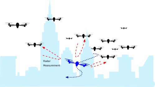
Figure 1: Pictorial representation of a DRN considered in this paper.

Today, current technological solutions are mainly based on surface-sited (terrestrial) and fixed radars, as battlefield radars, bird detection radars, perimeter surveillance radars, or high-resolution short-range radars, adopted in critical areas (e.g., airports) (see [7, 9, 8, 10, 11, 12] and the references therein). The possibility of monitoring the movement of small-sized UAVs using a multi-functional airfield radar is considered in [11]. In [13, 14, 15], the detection and localization performance of frequency-modulated continuous-wave (FMCW) radar systems is discussed. In [12], a joint connectivity and navigation problem is considered when the radar receiver is mounted on UAVs while the transmitter is on the ground in a multi-static configuration. In [16], a network of UAVs is used to track ground vehicles.

Nevertheless, the tracking of a malicious UAV with conventional terrestrial radars poses some difficulties since UAVs might be of small size and concealed within the UAV swarm, implying a low probability of being detected and tracked. For these reasons, differently from the literature and from our previous works [17, 18, 19], where usually radar sensor networks and UAVs are treated separately, this paper aims at introducing the concept of a monostatic dynamic radar network (DRN) consisting of UAVs carrying scanning radars of small sizes and weights, able to track a target and, simultaneously, adapt their formation-navigation control based on the quality of the signals backscattered by a non-cooperative (passive) flying target present in the environment. The considered network interrogates the surrounding via echoing signals, estimates and exchanges some target position-related information (e.g., ranging, bearing, and/or Doppler shifts), and jointly infers the target’s current position and velocity. The proposed scenario is displayed in Fig. 1 where each UAV individually exchanges measurements with neighboring UAVs and takes navigation decisions on-the-fly in order to reduce the uncertainty on target tracking.

In order to realize the aforementioned UAV-DRN, on-board radar technology should be chosen according to the UAV size and maximum payload. To this end, a promising solution might be to use millimeter wave (mm-wave) radar technology because of the possibility to miniaturize it for an on-board system and for its ranging accuracy and precision thanks to its larger available bandwidth [20, 21]. Furthermore, a MIMO solution can be employed due to its small size, which will resul in a highly directional radiation pattern (up to $1$-degree angular accuracy [20]). For example, in [21], FMCW radar sensors working at $77$ GHz are proposed for automotive applications. Moreover, when considering a target whose size is comparable to that of a mini/micro-UAV, FMCW scanning radars are usually preferred compared to pulse radars that perform poorly in localizing small radar cross sections [11]. For this reason, some research activities have focused on the assessment of the RCS values of drones and their impact on the detection performance [7, 22]. However, how the target RCS affects tracking accuracy and navigation performance is an open issue.

Another challenge in the realization of a UAV-DRN is the design of optimized paths for the UAVs to track malicious targets in the best possible way. The optimization of UAV trajectories has been the subject of numerous research studies [23, 24, 25, 26, 27, 28, 29, 30, 31, 32, 33, 34]. In regard to control design, many works in the literature have focused on optimal sensor/anchor placement [23], while others tackle the problem from an optimal control point-of-view [34]. Among other approaches, information-seeking optimal control (e.g., strategies driven by Shannon or Fisher information measures) has been extensively investigated for localization and tracking applications [30, 28, 26, 31, 32, 33, 27]. However, these solutions usually do not account for dynamics of the environment and a-priori define the entire paths, and, thus, they are not suitable for our scenario where UAVs should plan their trajectory in accordance to the movements of the unauthorized flying target.

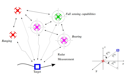
Figure 2: A UAV network, where different groups of UAVs acquire radar measurements. On the left, starting from the environment echo, the red UAVs estimate ranging information, the magenta the direction of arrival, and the green has full sensing capabilities (including the possibilities of inferring Doppler shifts). On the right, there is the used coordinate system.

Therefore, the aim of this paper is to study a UAV DRN as a cooperative radar sensing network for jointly tracking a non-authorized UAV in real-time and with high-accuracy and for smartly navigating the environment in order to reduce the correspondent tracking error (via multi-hop exchange of information). The design of DRNs, where the sensors and the target are flying (hence, mobile) poses new challenging issues because of their reconfigurability and mobility, but also offers an unprecedented level of flexibility for target tracking systems thanks to an increased degrees of freedom. Since not all the paths are the same from an information gathering point-of-view, the navigation will be formulated as a 3D optimization problem where an information-theoretic cost function permits to combine the a-priori information given by the history of measurements and the contributions brought by the currently acquired data, that can be delayed by the number of hops (and, hence, they can be aged). The impact of the RCS of small target (e.g., micro-UAV) will be taken into consideration in the measurement noise model, and in assessing the estimation accuracy.

The rest of the paper is organized as follows: Sec. II describes the problem, Sec. III reports details about the radar signal model and the tracking of a non-cooperative UAV, Sec. IV derives the cost function for optimizing the UAV navigation, Sec. V provides a possible solution for the optimization problem, and Sec. VI describes some simulations results.

Notation: Vectors and matrices are denoted by bold lowercase and uppercase letters, respectively; $[\mathbf{X}]_{ij}$ denotes the $(i,j)$-th entry of the matrix $\mathbf{X}$; $f\left(x\right)$ symbolizes a probability density function (pdf) of a continuous random variable $x$; $f\left(x\lvert z\right)$ is the conditional distribution of $x$ given $z$; $\mathbf{x}\sim\mathcal{N}\left(\bm{\mu},\bm{\Sigma}\right)$ means that $\mathbf{x}$ is distributed according to a Gaussian pdf with mean $\bm{\mu}$ and covariance matrix $\bm{\Sigma}$; ${x}\sim\mathcal{U}\left[a,b\right]$ denotes that ${x}$ is a uniform random variable with support $\left[a,b\right]$; $\mathbb{E}\left\{\cdot\right\}$ represents the expectation of the argument; $\left[\cdot\right]^{\mathsf{T}}$ denotes transposition of the argument. Finally, $\mathbf{I}_{n\times m}$ and $\mathbf{0}_{n\times m}$ indicate the identity and zero matrices of $n\times m$ size, respectively.

II Problem Statement

We consider a DRN of $N$ UAVs acting as mobile reference nodes (that is, with a-priori known positions, for instance available from GPS) that navigate through an outdoor environment in order to optimize the accuracy in tracking the position, $\mathbf{p}_{0}^{(k)}$, and the velocity, $\mathbf{v}_{0}^{(k)}$, of a moving non-cooperative target. The time is discrete and indexed with the symbol $k$.

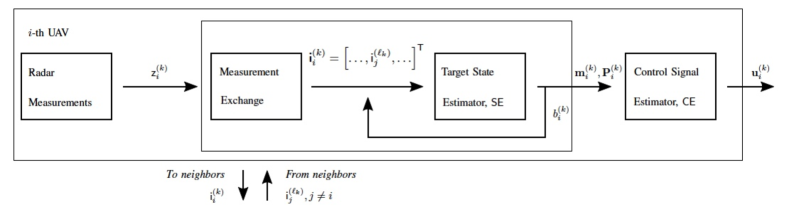
Figure 3: A block-diagram for decentralized joint tracking and navigation at the $i$-th UAV.

The mobility model of UAVs can be considered deterministic as the UAVs are flying outdoors (and, hence, they access the GPS signal with a high degree of accuracy) and, at each time instant, the next position of the $i$-th UAV is given by $\mathbf{p}_{i}^{(k+1)}=\varphi\left(\mathbf{p}_{i}^{(k)},\mathbf{u}_{i}^{(k)}\right)$, where $\varphi\left(\cdot\right)$ is the transition function, $\mathbf{p}_{i}^{(k)}=\left[x_{i}^{(k)},y_{i}^{(k)},z_{i}^{(k)}\right]^{\mathsf{T}}$ is the position of the $i$-th UAV at time instant $k$, and $\mathbf{u}_{i}^{(k)}=\left[u_{\mathsf{x},i}^{(k)},u_{\mathsf{y},i}^{(k)},u_{\mathsf{z},i}^{(k)}\right]^{\mathsf{T}}=g\left(v_{i}^{(k)},\Psi_{i}^{(k)},\Theta_{i}^{(k)}\right)$ is the control signal that the $i$-th UAV computes on its own for accurate tracking of the target [24]. The magnitude of the speed, the heading and the tilt angles are denoted by $v_{i}^{(k)}$, $\Psi_{i}^{(k)}$, and $\Theta_{i}^{(k)}$, respectively. In particular, the update of the position is given by

$$\left[\begin{array}[]{l}x_{i}^{(k+1)}\\ y_{i}^{(k+1)}\\ z_{i}^{(k+1)}\end{array}\right]=\left[\begin{array}[]{l}x_{i}^{(k)}+u_{\mathsf{x},i}^{(k)}\\ y_{i}^{(k)}+u_{\mathsf{y},i}^{(k)}\\ z_{i}^{(k)}+u_{\mathsf{z},i}^{(k)}\end{array}\right]=\left[\begin{array}[]{l}x_{i}^{(k)}+{\left(v_{i}^{(k)}\cdot\Delta t\right)\,\cos\left(\Psi_{i}^{(k)}\right)\,\sin\left(\Theta_{i}^{(k)}\right)}\\ y_{i}^{(k)}+{\left(v_{i}^{(k)}\cdot\Delta t\right)\,\sin\left(\Psi_{i}^{(k)}\right)\sin\left(\Theta_{i}^{(k)}\right)}\\ z_{i}^{(k)}+{\left(v_{i}^{(k)}\cdot\Delta t\right)\,\cos\left(\Theta_{i}^{(k)}\right)}\end{array}\right]\,,$$ (10)

with $\Delta t$ being the time interval between $k$ and $k+1$. To make the model more realistic, three constraints are added to impose the minimum and maximum speed and a maximum turn rate in both azimuthal and elevation planes [26], that are

$$\begin{cases}\,\,v_{\mathsf{min}}\leq v_{i}^{(k)}\leq v_{\mathsf{max}},\\ \,\,\big{\lvert}{\Psi_{i}^{(k)}-\Psi_{i}^{(k-1)}}\big{\rvert}\leq\Psi_{\mathsf{max}},\\ \,\,\big{\lvert}{\Theta_{i}^{(k)}-\Theta_{i}^{(k-1)}}\big{\rvert}\leq\Theta_{\mathsf{max}},\\ \end{cases}$$ (11)

where $v_{\text{min}}$ and $v_{\text{max}}$ are the minimum and maximum UAV speeds, respectively, and $\Psi_{\mathsf{max}}$ and $\Theta_{\mathsf{max}}$ are the turn rate limits, respectively. The geometry of the system in depicted in Fig. 2.

On the other hand, the target state vector at time instant $k$ is defined as $\mathbf{s}^{(k)}=\left[\left(\mathbf{p}_{0}^{(k)}\right)^{\mathsf{T}},\,\left(\mathbf{v}_{0}^{(k)}\right)^{\mathsf{T}}\right]^{\mathsf{T}}$, where the target position expressed in relation to the $i$-th UAV position at time instant $k$ is

$$\mathbf{p}_{0}^{(k)}\!\!=\!\!\left[\begin{array}[]{l}x_{0}^{(k)}\\ y_{0}^{(k)}\\ z_{0}^{(k)}\end{array}\right]\!\!=\!\!\left[\begin{array}[]{l}\!x_{i}^{(k)}\!+\!d_{i}^{(k)}\,\sin\left(\theta_{i}^{(k)}\right)\,\cos\left(\phi_{i}^{(k)}\right)\!\!\\ \!y_{i}^{(k)}\!+\!d_{i}^{(k)}\,\sin\left(\theta_{i}^{(k)}\right)\,\sin\left(\phi_{i}^{(k)}\right)\!\!\\ \!z_{i}^{(k)}\!+\!d_{i}^{(k)}\,\cos\left(\theta_{i}^{(k)}\right)\!\!\end{array}\right]\!\!,$$ (18)

where $d_{i}^{(k)}=\lVert\mathbf{p}_{0}^{(k)}-\mathbf{p}_{i}^{(k)}\rVert_{2}$ is the distance between the $i$-th UAV and the target at time instant $k$, and $\mathbf{v}_{0}^{(k)}=\left[v_{\mathsf{x},0}^{(k)},\,v_{\mathsf{y},0}^{(k)},\,v_{\mathsf{z},0}^{(k)}\right]^{\mathsf{T}}$ is its velocity. The state evolves according to the following dynamic model,

$$\mathbf{s}^{(k+1)}=\mathbf{A}^{(k)}\,\mathbf{s}^{(k)}+\mathbf{q}^{(k)},$$ (19)

where $\mathbf{A}^{(k)}$ is the transition matrix, which is assumed known, and $\mathbf{q}^{(k)}\sim\mathcal{N}\left(\mathbf{0},\mathbf{Q}^{(k)}\right)$ is the process noise.

All UAVs perform radar measurements with respect to the target, and starting from the acquired data, they can estimate Doppler shifts, ranging and/or bearing from which the position and the velocity of the target can finally be estimated at each time step (two-step localization) through cooperation [35]. In fact, starting from the radar received signals, the Doppler shift and ranging information can be inferred given the beat frequency estimation [15]; whereas the direction-of-arrival (DOA) can be associated with the antenna steering direction. More specifically, UAV rotations might be exploited to point the on-board radar antenna in different angular directions and to form a received signal strength (RSS) pattern after each rotation as in [36]. As an alternative, one may consider a MIMO radar system with electronic beamforming capabilities [10]. Hence, each UAV can process the collected measurements in different ways: we indicate with $\mathcal{N}_{\mathsf{r}}$ the set of UAVs acquiring ranging estimates, $\mathcal{N}_{\mathsf{d}}$ the set able to collect Doppler shifts, $\mathcal{N}_{\mathsf{b}}$ the set inferring bearing data, and $\mathcal{N}_{\mathsf{j}}$ the set able to estimate all the parameters. The network composed of UAVs with heterogeneous capabilities is indicated with $\mathcal{N}=\mathcal{N}_{\mathsf{r}}\cup\mathcal{N}_{\mathsf{d}}\cup\mathcal{N}_{\mathsf{b}}\cup\mathcal{N}_{\mathsf{j}}$.

In accordance with Fig. 3, the $i$-th UAV performs the following steps at time instant $k$:

Measurement step

The first task is to retrieve state-related information from radar measurements, i.e., from the signal backscattered by the environment where the malicious target navigates. In Fig. 3, we indicate with $\mathsf{z}_{i}^{(k)}$ the estimates inferred by the $i$-th UAV at time instant $k$;

Communication step

Once the $i$-th UAV obtains its own estimates, it communicates this information to the neighbors together with its own position $\left(\text{defined as\,\,}\mathsf{i}_{i}^{(k)}=\left[\mathsf{z}_{i}^{(k)},\mathbf{p}_{i}^{(k)}\right]\right)$, and it receives back the same data from neighboring UAVs via multi-hop propagation, i.e., $\mathsf{i}_{j}^{(\ell_{k})}=\left[\mathsf{z}_{j}^{(\ell_{k})},\mathbf{p}_{j}^{(\ell_{k})}\right]$, where $\ell_{k}$ is a time index accounting for the delay due to multi-hops [17, 18, 37]. Each node can directly communicate with its neighbors within a radius of length $r_{\mathsf{max}}$, while for greater distances, the information is delayed by $h_{ij}^{(k)}$ time slots, equal to the number of hops between the $i$-th and $j$-th UAV at instant $k$. We indicate with $\mathcal{N}_{\mathsf{nb},i}^{(k)}$ the set of neighbors of the $i$-th UAV at time instant $k$. Due to multi-hop propagation, the information obtained at each UAV can be aged, preventing an updated view of the network. Finally, we gather all the acquired data in $\bm{\mathsf{i}}_{i}^{(k)}$, which is the vector that contains the estimates and locations of the $i$-th UAV and its neighbors.

Target Tracking

Given the measurements and the positions of the other UAVs, the presence of a malicious target can be detected and its state can be tracked by each UAV. A Bayesian estimator can be used to compute the a-posteriori probability distribution of the target state given the acquired information (the belief is denoted with $b_{i}^{(k)}\left(\mathbf{s}^{(k)}\right)$ in Fig. 3). In our case, we adopt an Extended Kalman Filter (EKF) algorithm to compute the Gaussian belief of the state as $b_{i}^{(k)}\left(\mathbf{s}^{(k)}\right)=f\left(\mathbf{s}^{(k)}\lvert\bm{\mathsf{i}}_{i}^{(1:k)}\right)\overset{\mathrm{EKF}}{=}\mathcal{N}\left({\mathbf{m}_{i}^{(k)}},{\mathbf{P}_{i}^{(k)}}\right)$, where ${\mathbf{m}_{i}^{(k)}}$ and ${\mathbf{P}_{i}^{(k)}}$ are the conditional mean vector and the covariance matrix of the state and $\bm{\mathsf{i}}_{i}^{(1:k)}$ is the acquired information by the $i$-th UAV up to time instant $k$. The EKF filter algorithm produces estimates that minimize the mean-squared estimation error conditioned on the history of acquired information. Consequently, the estimate of the state at time $k$, $\hat{\mathbf{s}}_{i}^{(k)}$, is defined as the conditional mean $\hat{\mathbf{s}}_{i}^{(k)}=\mathbf{m}_{i}^{(k\lvert k)}=\mathbb{E}\left\{\mathbf{s}^{(k)}\lvert\bm{\mathsf{i}}_{i}^{(1:k)}\right\}$. With reference to Fig. 3, we can write

$$\hat{\mathbf{s}}_{i}^{(k)} =\mathsf{SE}\left(\bm{\mathsf{i}}_{i}^{(k)},b_{i}^{(k-1)}\left(\mathbf{s}_{0}^{(k-1)}\right)\right)\overset{\mathrm{EKF}}{=}\mathsf{SE}\left(\bm{\mathsf{i}}_{i}^{(k)},\mathbf{m}_{i}^{(k-1)},\mathbf{P}_{i}^{(k-1)}\right),$$ (20)

with $\mathsf{SE}\left(\cdot\right)$ being a function describing the state estimator. Subsequently, an approach based on diffusion of information [39] can follow the tracking step to further enhance the estimation accuracy.

UAV control step

The last step is the control signal estimation by the $i$-th agent that will allow the UAV to reach its next position, $\mathbf{p}_{i}^{(k+1)}$, according to a given command, $\mathbf{u}_{i}^{(k)}$. Since the quality of the measurements depends on the DRN geometry and target position, the control law should properly change the UAV formation and position in order to maximize the quality of the tracking process and, at the same time, take into account physical constraints (e.g., obstacles). For this reason, at each time step, each UAV searches for the next UAV formation that minimizes an information-theoretic cost function at the next time instant, that can be written as

$$\left(\mathbf{L}_{i}^{(k+1)}\right)^{\star}= \operatorname*{argmin}_{\mathbf{L}_{i}^{(k+1)}}\,\,\mathcal{C}\left(\mathbf{J}_{i}^{(k)}\left(\hat{\mathbf{p}}_{0;i}^{(k+1\lvert k)},\,\mathbf{L}_{i}^{(k+1)}\right)\right),$$ (21)

where $\mathbf{L}_{i}^{(k)}=\left[\ldots,\mathbf{p}_{j}^{(\ell_{k})},\ldots\right]^{\mathsf{T}}$, $j\in\mathcal{N}_{\mathsf{nb},i}^{(k)}$, is the vector containing the locations of UAVs that are neighbors of the $i$-th UAV at time instant $k$ (those belonging to the set $\mathcal{N}_{\mathsf{nb},i}^{(k)}$), $\ell_{k}=k-h_{ij}^{(k)}+1$ is the time instant associated with the exchanged information due to multi-hops, $\mathcal{C}\left(\cdot\right)$ is a function that will be defined in the sequel, $\mathbf{J}_{i}^{(k)}$ is the cost function also defined in the next, and $\hat{\mathbf{p}}_{0;i}^{(k+1\lvert k)}=\left[\hat{\mathbf{s}}_{i}^{(k+1\lvert k)}\right]_{1:3}$ is the predicted target position where $\hat{\mathbf{s}}_{i}^{(k+1\lvert k)}$ is derived during the prediction step of (20).

Then, recalling the transition model (10), the control signal of the $i$-th UAV that satisfies (21) is given by $\mathbf{u}_{i}^{(k)}=\left[\left(\mathbf{L}_{i}^{(k+1)}\right)^{\star}\right]_{i}-\mathbf{p}_{i}^{(k)}$, where $\left[\cdot\right]_{i}$ is an operator that picks the $i$-th entry of the optimal formation in (21).

According to the D-optimality criterion described in [30], we choose the following cost function:

$$\mathcal{C}\left(\mathbf{J}_{i}^{(k)}\left(\mathbf{p}_{0}^{(k)},\mathbf{L}_{i}^{(k)}\right)\right)=-\ln\det\left(\mathbf{J}_{i}^{(k)}\left(\mathbf{p}_{0}^{(k)};\mathbf{L}_{i}^{(k)}\right)\right),$$ (22)

where $\text{det}\left(\cdot\right)$ is the determinant operator, and $\mathbf{J}_{i}^{(k)}\left(\mathbf{p}_{0}^{(k)};\mathbf{L}_{i}^{(k)}\right)$ is the information matrix of the target’s location as a function of the current and previous locations of the neighboring UAVs. Following the same principle as in [26], we consider the posterior covariance matrix in its inverse (information) form as

$$\mathbf{J}_{i}^{(k)}\left(\mathbf{p}_{0}^{(k)};\mathbf{L}_{i}^{(k)}\right)=\left[\left(\mathbf{P}_{i}^{(k\lvert k)}\right)^{-1}\right]_{11},$$ (23)

where the operator $\left[\cdot\right]_{11}$ picks the sub-matrix relative to the target position, and with the covariance matrix defined as

$$\mathbf{P}_{i}^{(k\lvert k)} =\left[\begin{array}[]{cc}\mathbf{P}_{\mathsf{pp},i}^{(k\lvert k)}&\mathbf{P}_{\mathsf{pv},i}^{(k\lvert k)}\\ \mathbf{P}_{\mathsf{vp},i}^{(k\lvert k)}&\mathbf{P}_{\mathsf{vv},i}^{(k\lvert k)}\end{array}\right],$$ (26)

whose diagonal contains the variances of the position and the velocity estimates. The cost function defined in (22) requires knowledge of the actual target position which is the unknown parameter to be estimated, and for this reason (21) is evaluated at the position estimate available to the $i$-th UAV at time instant $k$.

Finally, we consider that the problem is subjected to the following set of constraints:

$$\begin{cases}\,\,d_{ij}^{(k)}\geq d_{\mathsf{U}}^{*},\,\,d_{i}^{(k)}\geq d_{\mathsf{T}}^{*},\,\,\mathcal{T}_{i}\cap\mathcal{O}=\varnothing,\\ \,\,v_{\mathsf{min}}\leq v_{i}^{(k)}\leq v_{\mathsf{max}},\,\,\,\,\,\,\,\,\,\,\,\,\,\quad\,\,\,\,\qquad\quad\,\,\,\\ \lvert\Psi_{i}^{(k+1)}-\Psi_{i}^{(k)}\rvert\leq\Psi_{\mathsf{max}},\\ \lvert\Theta_{i}^{(k+1)}-\Theta_{i}^{(k)}\rvert\leq\Theta_{\mathsf{max}},\end{cases}$$ (27)

for $i,j=1,\ldots,N$, and where $d_{ij}^{(k)}$ is the inter-UAV distance, $d_{\mathsf{U}}^{*}$ is the anti-collision safety distance among UAVs, $d_{\mathsf{T}}^{*}$ is the safety distance with respect to the target, $\mathcal{T}_{i}$ is the set of feasible position points of the trajectory of the $i$-th UAV, and $\mathcal{O}$ is the set of obstacles present in the environment from which the UAVs should keep a safety distance equal to $d_{\mathsf{O}}^{*}$.

III UAV-Target Tracking

The target tracking aims to estimate the state of the target (e.g., its position and velocity) starting from the received echo signals. In this section, we briefly recall the signal model used by a FMCW radar that might be integrated in the UAV payload and, then, we focus on a Bayesian filtering method for target tracking. More specifically, we adopt an EKF as a tool to solve the tracking problem thanks to its capability of dealing with heterogeneous measurements, statistical characterization of uncertainties, and UAV mobility models.

III-A Example of Signal Model for on-board FMCW Radar

A widely used radar technology for UAVs is the FMCW radar that, differently from pulse radars, interrogates the environment with a signal linearly modulated in frequency (namely, chirp). Sometimes, in order to increase the signal-to-noise ratio (SNR) and infer Doppler shift measurements, multiple chirps can be transmitted in a fixed time window (chirp train). Once the signal is received back by the radar, it is combined with a template of the transmitted waveform by a mixer. As a result, different target-related parameters, such as ranging and Doppler shifts, can be inferred by processing the frequency and phase information of the signal at the output of this mixer. In particular, to retrieve velocity information, it is possible to rely on phase differences between different received chirps, or, directly, on Doppler-shift estimates. If the FMCW radar consists of multiple transmitting and receiving antennas (MIMO radar), the angle-of-arrival can be estimated through the measurement of phase differences between the antennas. Another possibility is to exploit the UAV rotations: by rotating the on-board antenna towards ad-hoc steering directions, the direction of arrival can be inferred by considering the maximum power of the received echoes.

A promising solution for UAV integration is to operate at millimeter-waves so that FMCW radars can be miniaturized and equipped with multiple antennas. By working at high frequencies, a resolution smaller than a millimeter can be obtained thanks to the higher available bandwidth, up to $4$ GHz at $77$ GHz. Example of FMCW for UAVs can be found in [10] and the references therein.

For the following analysis and in order to derive a suitable observation model for the tracking algorithm, it is important to characterize the noise uncertainties of the ranging, bearing, and Doppler shift estimates as inferred by the radar. To this end, the Cramér-Rao lower bound (CRLB) expression, which can be viewed as the minimum variance achievable by an unbiased estimator, can be considered for ranging and Doppler shift estimates, given by [40, 41]

$$\text{var}\left(d_{i}^{(k)}\right)\geq\frac{3}{2}\,\left(\frac{2\,c}{\gamma}\right)^{2}\frac{1}{\left(2\,\pi\,B_{i}\right)^{2}\,\mathsf{SNR}_{i}^{(k)}},\quad\text{var}\left(f_{\mathsf{d},i}^{(k)}\right)\geq\frac{1}{\left(2\,\pi\right)^{2}}\frac{6}{T_{i}^{2}\,\,\mathsf{SNR}_{i}^{(k)}},$$ (28)

where $T_{i}=\tau_{i}\,M_{i}$ is the observation time, $\tau_{i}$ is the time sweep of a single sawtooth, $B_{i}$ is the frequency sweep, $M_{i}$ is the number of chirps (processing gain), $\gamma=4$ is the path-loss exponent for two-way (radar) channel, $c$ is the speed-of-light, and the SNR is defined as

$$\mathsf{SNR}_{i}^{(k)}=\frac{\lambda^{2}\,P_{\mathsf{t}}\,G^{2}\left(\Theta_{b}\right)}{\left(4\pi\right)^{3}\,P_{\mathsf{n}}}\times\frac{\rho}{\left(d_{i}^{(k)}\right)^{\gamma}}=\mathsf{SNR}_{0}\times\frac{\rho}{\left(d_{i}^{(k)}\right)^{\gamma}}$$ (29)

where $\rho$ is the target RCS, $\mathsf{SNR}_{0}$ is the SNR evaluated at $d_{0}=1$ m and $\rho_{0}=1$ m², $\lambda$ is the wavelength, $P_{\mathsf{t}}$ is the transmitted power, $G\left(\Theta_{b}\right)$ is the antenna gain pointing at $\Theta_{b}=(\theta_{b},\phi_{b})$, $P_{\mathsf{n}}=N_{0}\,B_{i}$ is the noise power with $N_{0}=\kappa_{\mathsf{b}}\,T_{0}\,F$, $\kappa_{\mathsf{b}}$ is the Boltzmann constant, $T_{0}$ is the receiver temperature, and $F$ is the receiver noise figure.

On the other hand, for the bearing case, we suppose that the noise uncertainty (in terms of standard deviation) is constant in the azimuthal and elevation planes and coincides with the Half Power Beamwidth (HPBW) of the on-board antenna.

III-B Observation Model

As described in the previous section, starting from the received signal echoes, each UAV estimates information about the target state, e.g., the distance and angle from the target or the Doppler shift. Subsequently, such information is exchanged between UAVs via multi-hops together with the UAV positions. At the end of this communication step, each UAV puts together the gathered information, exploitable for target tracking in a vector. Let $\bm{\mathsf{i}}_{i}^{(k)}=\left[\ldots,\mathsf{i}_{j}^{(\ell_{k})},\ldots\right]^{\mathsf{T}}$ be the information available to the $i$-th UAV at time instant $k$, where the generic element $\mathsf{i}_{j}^{(\ell_{k})}=\left[\mathsf{z}_{j}^{(\ell_{k})},\mathbf{p}_{j}^{(\ell_{k})}\right]^{\mathsf{T}},$ $j\in\mathcal{N}_{\mathsf{nb},i}^{(k)}$, contains the radar estimates and the position of the $j$-th neighboring UAV delayed due to the multi-hop connection with the $i$-th agent. The generic radar measurement can be written as

$$\mathsf{z}_{i}^{(k)}=\mathrm{l}_{i}^{(k)}\,o_{i}^{(k)}+\left(1-\mathrm{l}_{i}^{(k)}\right)\,w_{i}^{(k)},$$ (30)

where $\mathrm{l}_{i}^{(k)}$ is a flag indicating the presence (if any) of a line-of-sight (LOS) link between the $i$-th UAV and the target, and $w_{i}^{(k)}$ is an outlier term due to the presence of multipath components or extremely noisy measurements [42]. The first term in (30) contains information about the target state, that is

$$o_{i}^{(k)}=h_{i}^{(k)}\left(\mathbf{s}^{(k)}\right)+n_{i}^{(k)},$$ (31)

where $h_{i}^{(k)}$ is a function that relates the data to the target state and whose expression depends on the UAV sensing and processing capabilities, i.e.,

$$h_{i}^{(k)}=\begin{cases}\frac{\gamma}{2}d_{i}^{(k)}=\frac{\gamma}{2}\,\Big{\lVert}\mathbf{p}_{0}^{(k)}-\mathbf{p}_{i}^{(k)}\Big{\rVert}_{2},\,\,\,\,\,\text{if $i\in\mathcal{N}_{\mathsf{r}}\vee\mathcal{N}_{\mathsf{j}}$},\\ \phi_{i}^{(k)}=\text{tan}^{-1}\left({y_{0i}^{(k)}}/{x_{0i}^{(k)}}\right),\quad\text{if $i\in\mathcal{N}_{\mathsf{b}}\vee\mathcal{N}_{\mathsf{j}}$},\\ \theta_{i}^{(k)}=\text{cos}^{-1}\left({z_{0i}^{(k)}}/{d_{i}^{(k)}}\right),\quad\text{if $i\in\mathcal{N}_{\mathsf{b}}\vee\mathcal{N}_{\mathsf{j}}$},\\ f_{\mathsf{d},i}^{(k)}=\left({\gamma\,v_{\mathsf{rad},i}^{(k)}}/{2\,\lambda}\right),\quad\quad\,\,\,\,\text{if $i\in\mathcal{N}_{\mathsf{d}}\vee\mathcal{N}_{\mathsf{j}}$},\end{cases}$$ (32)

where $d_{i}^{(k)}$, $\phi_{i}^{(k)}$, $\theta_{i}^{(k)}$, and $f_{\mathsf{d},i}^{(k)}$ are the actual distance, azimuth, elevation, and Doppler shift between the $i$-th UAV and the target, $v_{\mathsf{rad},i}^{(k)}$ is the radial velocity, $\vee$ is the or-operator, and $x_{0i}^{(k)}=x_{0}^{(k)}-x_{i}^{(k)}$, $y_{0i}^{(k)}=y_{0}^{(k)}-y_{i}^{(k)}$, and $z_{0i}^{(k)}=z_{0}^{(k)}-z_{i}^{(k)}$.

The measurement noise in (31) is modeled as $n_{i}^{(k)}\sim\mathcal{N}\left(0,\left(\sigma_{i}^{(k)}\right)^{2}\right)$, where, in accordance with the type of measurement, the ranging and Doppler shift variances are described by the CRLB as in (28), that can be reformulated as

$$\left(\sigma_{\mathsf{r},i}^{(k)}\right)^{2}=\sigma_{\mathsf{r},0}^{2}\,\frac{\left(d_{i}^{(k)}\right)^{\gamma}}{\rho},\quad\left(\sigma_{\mathsf{d},i}^{(k)}\right)^{2}=\sigma_{\mathsf{d},0}^{2}\,\frac{\left(d_{i}^{(k)}\right)^{\gamma}}{\rho},$$ (33)

where $\sigma_{\mathsf{r},0}^{2}$ and $\sigma_{\mathsf{d},0}^{2}$ are the variances at the reference distance $d_{i}^{(k)}=1$ m and with a target RCS of $\rho=1$ m². On the contrary, the bearing noise variance is constant with respect to the distance and the target RCS, and ${\sigma}^{2}_{\mathsf{b},0}$ is related to the radar HPBW, as previously stated.

Eq. (30) can be written in vector form as

$$\bm{\mathsf{z}}_{i}^{(k)}=\bm{\mathrm{l}}_{i}^{(k)}\odot\left(\mathbf{h}_{i}^{(k)}\left(\mathbf{s}^{(k)}\right)+\mathbf{n}_{i}^{(k)}\right)+(1-\bm{\mathrm{l}}_{i}^{(k)})\odot\mathbf{w}_{i}^{(k)},$$ (34)

where $\odot$ is the Hadamard product, and the noise can be described as $\mathbf{n}_{i}^{(k)}\sim\mathcal{N}\left(\mathbf{0},\mathbf{R}_{i}^{(k)}\right)$ with a covariance matrix given by $\mathbf{R}_{i}^{(k)}=\text{diag}\left(\ldots,\left(\sigma_{j}^{(\ell_{k})}\right)^{2},\ldots\right)$.

III-C UAV-Target Tracking

Starting from the transition and measurement model previously described, each UAV can perform tracking to estimate the state of the target. Within this framework, the main goal of each UAV is to infer the full joint posterior probability of the state at time instant $k$, $\mathbf{s}^{(k)}$, given the available information up to the current time instant, namely $\bm{\mathsf{i}}_{i}^{(1:k)}$.

In this context, it is possible to define a probabilistic state-space Markovian model by considering the following statistical models:

• Measurement model. It describes how the state is related to the available information by the likelihood $f\left(\bm{\mathsf{i}}_{i}^{(k)}\lvert\mathbf{s}^{(k)}\right)=f\left(\bm{\mathsf{z}}_{i}^{(k)}\lvert\mathbf{s}^{(k)}\right)$, defined by the statistical measurement model in (34);

• State transition model. It describes how the state evolves in time, in accordance with the dynamic model in (19) and given by $f\left(\mathbf{s}^{(k)}\lvert\mathbf{s}^{(k-1)}\right)$.

$$\mathbf{J}_{\mathsf{pp},i}^{(k\lvert k)}\left(\mathbf{p}_{0}^{(k)};\mathbf{L}_{i}^{(k)}\right)= \sum_{j=1}^{\lvert\mathcal{N}_{\mathsf{nb},i}^{(k)}\rvert}\mathrm{l}_{j}^{(\ell_{k})}\left[\frac{\kappa_{j}}{\left(\sigma_{\mathsf{r},j}^{(\ell_{k})}\right)^{2}}\,\mathbf{G}_{\mathsf{r},j}^{(\ell_{k})}\left(\mathbf{p}_{0}^{(k)};\mathbf{p}_{j}^{(\ell_{k})}\right)+\frac{\xi_{j}}{\left(\sigma_{\mathsf{d},j}^{(\ell_{k})}\right)^{2}}\,\mathbf{G}_{\mathsf{d},j}^{(\ell_{k})}\left(\mathbf{p}_{0}^{(k)};\mathbf{p}_{j}^{(\ell_{k})}\right)\right.$$

$$\left.+\,\beta_{j}\left(\frac{1}{\left(\sigma_{\mathsf{\phi},j}^{(\ell_{k})}\right)^{2}}\,\mathbf{G}_{\mathsf{\phi},j}^{(\ell_{k})}\left(\mathbf{p}_{0}^{(k)};\mathbf{p}_{j}^{(\ell_{k})}\right)+\frac{1}{\left(\sigma_{\mathsf{\theta},j}^{(\ell_{k})}\right)^{2}}\,\mathbf{G}_{\mathsf{\theta},j}^{(\ell_{k})}\left(\mathbf{p}_{0}^{(k)};\mathbf{p}_{j}^{(\ell_{k})}\right)\right)\,\right],$$ (35)

 

Given this state-space model, an EKF approach can be used because the observation functions in (30) are non-linear and the noises are Gaussian distributed. In this case, each UAV performs the two main steps of the EKF algorithm: (1) A prediction step within which each UAV computes the predictive information $\left(\mathbf{m}_{i}^{(k\lvert k-1)},\mathbf{P}_{i}^{(k\lvert k-1)}\right)$ given a model for the target mobility as in (19); and (2) An update step for updating the mean and covariance $\left(\mathbf{m}_{i}^{(k\lvert k)},\mathbf{P}_{i}^{(k\lvert k)}\right)$ once a new measurement becomes available. The Jacobian matrix $\nabla\mathbf{h}_{i}^{(k)}$ is given by

$$\nabla\mathbf{h}_{i}^{(k)}=\left[\begin{array}[]{cc}\nabla_{\mathbf{p}_{0}^{(k)}}\left(\mathbf{h}_{\mathsf{r},i}^{(k)}\right)&\mathbf{0}\\ \nabla_{\mathbf{p}_{0}^{(k)}}\left(\mathbf{h}_{\mathsf{\phi},i}^{(k)}\right)&\mathbf{0}\\ \nabla_{\mathbf{p}_{0}^{(k)}}\left(\mathbf{h}_{\mathsf{\theta},i}^{(k)}\right)&\mathbf{0}\\ \nabla_{\mathbf{p}_{0}^{(k)}}\left(\mathbf{h}_{\mathsf{d},i}^{(k)}\right)&\nabla_{\mathbf{v}_{0}^{(k)}}\left(\mathbf{h}_{\mathsf{d},i}^{(k)}\right)\end{array}\right]_{\mathbf{s}^{(k)}=\mathbf{m}_{i}^{(k\lvert k-1)}},$$ (36)

where the generic elements in (36) are the derivatives of the measurement models in (30) with respect to the state, that is.

$$\nabla_{\mathbf{p}_{0}^{(k)}}\frac{\gamma}{2}\,\,d_{j}^{(\ell_{k})}=\frac{\gamma}{2}\,\mathbf{a}_{j}^{(\ell_{k})}\left(\phi_{j}^{(\ell_{k})},\theta_{j}^{(\ell_{k})}\right),$$ (37)

$$\nabla_{\mathbf{p}_{0}^{(k)}}\phi_{j}^{(\ell_{k})}=\mathbf{a}_{j}^{(\ell_{k})}\left(\phi_{j}^{(\ell_{k})}+\pi/2,\pi/2\right)/\left(d_{j}^{(\ell_{k})}\,\sin(\theta_{j}^{(\ell_{k})})\right),$$ (38)

$$\nabla_{\mathbf{p}_{0}^{(k)}}\theta_{j}^{(\ell_{k})}=\mathbf{a}_{j}^{(\ell_{k})}\left(\phi_{j}^{(\ell_{k})},\theta_{j}^{(\ell_{k})}+\pi/2\right)/\left(d_{j}^{(\ell_{k})}\right),$$ (39)

$$\nabla_{\mathbf{v}_{0}^{(k)}}f_{\mathsf{d},j}^{(\ell_{k})}=\frac{\gamma}{2\,\lambda}\,\mathbf{a}_{j}^{(\ell_{k})}\,\left(\phi_{j}^{(\ell_{k})},\theta_{j}^{(\ell_{k})}\right),$$ (40)

where $\mathbf{a}_{j}^{(\ell_{k})}=\left[\mathsf{c}_{\phi,j}^{(\ell_{k})}\,\mathsf{s}_{\theta,j}^{(\ell_{k})},\mathsf{s}_{\phi,j}^{(\ell_{k})}\,\mathsf{s}_{\theta,j}^{(\ell_{k})},\mathsf{c}_{\theta,j}^{(\ell_{k})}\right]^{\mathsf{T}}$ is the direction vector and where the following notation has been adopted: $\mathsf{c}_{\alpha,i}^{(k)}=\cos\left(\alpha_{i}^{(k)}\right)$, $\mathsf{s}_{\alpha,i}^{(k)}=\sin\left(\alpha_{i}^{(k)}\right)$ with $\alpha_{i}^{(k)}$ being the azimuth/elevation angle in the set $\left\{\phi_{i}^{(k)},\theta_{i}^{(k)}\right\}$. Finally, we have

$$\nabla_{x_{0}^{(k)}}f_{\mathsf{d},j}^{(\ell_{k})}=\frac{\gamma}{2\,\lambda}\left(-\mathsf{s}_{\phi,j}^{(\ell_{k})}\,\mathsf{s}_{\theta,j}^{(\ell_{k})}\,\omega_{\mathsf{z}}+\mathsf{c}_{\theta,j}^{(\ell_{k})}\,\omega_{\mathsf{y}}\right)\,,$$

$$\nabla_{y_{0}^{(k)}}f_{\mathsf{d},j}^{(\ell_{k})}=\frac{\gamma}{2\,\lambda}\left(\mathsf{c}_{\phi,j}^{(\ell_{k})}\,\mathsf{s}_{\theta,j}^{(\ell_{k})}\,\omega_{\mathsf{z}}-\mathsf{c}_{\theta,j}^{(\ell_{k})}\,\omega_{\mathsf{x}}\right)\,,$$

$$\nabla_{z_{0}^{(k)}}f_{\mathsf{d},j}^{(\ell_{k})}=\frac{\gamma}{2\,\lambda}\left(-\mathsf{c}_{\phi,j}^{(\ell_{k})}\,\mathsf{s}_{\theta,j}^{(\ell_{k})}\,\omega_{\mathsf{y}}+\mathsf{s}_{\phi,j}^{(\ell_{k})}\,\mathsf{s}_{\theta,j}^{(\ell_{k})}\,\omega_{\mathsf{x}}\right)\,,$$ (41)

where the 3D angular velocity is given by

$$\bm{\omega}_{i}^{(k)} =\left[\omega_{\mathsf{x}},\,\omega_{\mathsf{y}},\,\omega_{\mathsf{z}}\right]^{\mathsf{T}}=\frac{\left(\mathbf{p}_{0}^{(k)}-\mathbf{p}_{i}^{(k)}\right)\times\left(\mathbf{v}_{0}^{(k)}-\mathbf{v}_{i}^{(k)}\right)}{\left(d_{i}^{(k)}\right)^{2}},$$ (42)

where $\times$ indicates the cross product between the two vectors. If a measurement is not available (e.g., when a drone collects only ranging information), the correspondent row is eliminated from (36).

IV Information-Theoretic Cost Function

The autonomous control in (21) is designed to estimate the next location of each UAV in order to maximize its capability to best track the target, considering also the locations and estimates of the neighboring UAVs. The tracking performance mainly depends on the prior information acquired (if present), on the UAV network formation (geometry) and on the uncertainty of the collected measurements.

In this section, we aim at deriving the analytical expression of the information matrix $\mathbf{J}_{i}^{(k)}\left(\cdot\right)$ in (22). Starting from the information model described in Sec. III-B and from the output of the EKF, it is possible to write the information matrix for the dynamic scenario as [23]

$$\mathbf{J}_{i}^{(k)}\left(\mathbf{p}_{0}^{(k)};\mathbf{L}_{i}^{(k)}\right)=\left[\mathbf{P}_{i}^{-}-\mathbf{P}_{i}^{-}\,\,\nabla^{\mathsf{T}}\mathbf{h}_{i}^{(k)}\,\left(\mathbf{S}_{i}^{(k)}\right)^{-1}\,\nabla\mathbf{h}_{i}^{(k)}\,\mathbf{P}_{i}^{-}\right]_{11}^{-1},$$ (43)

where $\mathbf{P}_{i}^{-}=\mathbf{P}_{i}^{(k\lvert k-1)}$ is the predictive covariance, $\nabla^{\mathsf{T}}\mathbf{h}_{i}^{(k)}$ is the Jacobian matrix defined in (36), $\mathbf{S}_{i}^{(k)}=\nabla\mathbf{h}_{i}^{(k)}\,\mathbf{P}_{i}^{-}\,\nabla^{\mathsf{T}}\mathbf{h}_{i}^{(k)}+\mathbf{R}_{i}^{(k)}$, and $\mathbf{R}_{i}^{(k)}$ is the covariance matrix that depends on the statistical characterization of the measurement noise.

Then, according to the matrix inversion lemma [43], (43) can be reformulated in a more convenient form as

$$\mathbf{J}_{i}^{(k)}\left(\mathbf{p}_{0}^{(k)};\mathbf{L}_{i}^{(k)}\right)\! =\left[\left(\mathbf{P}_{i}^{-}\right)^{-1}+\nabla^{\mathsf{T}}\mathbf{h}_{i}^{(k)}\left(\mathbf{R}_{i}^{(k)}\right)^{-1}\nabla\mathbf{h}_{i}^{(k)}\right]_{11}=\mathbf{J}_{\mathsf{pp},i}^{(k\lvert k-1)}+\mathbf{J}_{\mathsf{pp},i}^{(k\lvert k)},$$ (44)

where $\mathbf{J}_{\mathsf{pp},i}^{(k\lvert k-1)}=\left[\left(\mathbf{P}_{i}^{-}\right)^{-1}\right]_{11}$ is the sub-block matrix corresponding to the predictive information matrix of the target position, while $\mathbf{J}_{\mathsf{pp},i}^{(k\lvert k)}$ corresponds to the Fisher Information Matrix (FIM) for non-random parameters, that is,

$$\mathbf{J}_{\mathsf{pp},i}^{(k\lvert k)}\left(\mathbf{p}_{0}^{(k)};\mathbf{L}_{i}^{(k)}\right)=\nabla^{\mathsf{T}}_{\mathbf{p}_{0}^{(k)}}\mathbf{h}_{i}^{(k)}\left(\mathbf{R}_{i}^{(k)}\right)^{-1}\nabla_{\mathbf{p}_{0}^{(k)}}\mathbf{h}_{i}^{(k)}.$$ (45)

Equation (45) puts in evidence the relation of the information model (encapsulated in $\mathbf{R}_{i}^{(k)}$) and of the UAV-target geometric configuration (in the Jacobian matrix, $\nabla_{\mathbf{p}_{0}^{(k)}}\mathbf{h}_{i}^{(k)}$) on the localization performance. The deterministic FIM depends on the true target position and on the UAV locations as known by each UAV. Because this information is not available, they are substituted with their estimates. After some computation, it is possible to write (45) as in (III-C) with $\kappa_{j}=1$ if the $j$-th neighbor of the $i$-th UAV can process ranging information ($j\in\mathcal{N}_{\mathsf{r}}\vee\mathcal{N}_{\mathsf{j}}$), otherwise $\kappa_{j}=0$; similarly $\beta_{j}=1$ if bearing data are available at the $j$-th node ($j\in\mathcal{N}_{\mathsf{b}}\vee\mathcal{N}_{\mathsf{j}}$), and $\xi_{j}=1$ if $j\in\mathcal{N}_{\mathsf{d}}\vee\mathcal{N}_{\mathsf{j}}$. As we can see, (III-C) is composed of four main terms, each one carrying the position-related information from the corresponding measurements (ranging/bearing/Doppler). In turn, each term has a geometric component dependent on the UAV-target positions (the matrices $\mathbf{G}$) weighted by the measurement uncertainty (the factors $1/\sigma^{2}$). The latter are the inverse of the diagonal entries in the measurement covariance matrix $\mathbf{R}_{i}^{(k)}$, and are reported in (33). Thanks to the possibility to discriminate LOS/NLOS situations, we assume that the UAVs exactly know the values of the coefficients in (33). The geometric matrices in (III-C) are given by

$$\mathbf{G}_{\mathsf{r},j}^{(\ell_{k})}\left(\mathbf{p}_{0}^{(k)};\mathbf{p}_{j}^{(\ell_{k})}\right)=\frac{\gamma^{2}}{4}\,\nabla_{\mathbf{p}_{0}^{(k)}}^{\mathsf{T}}\left(d_{j}^{(\ell_{k})}\right)\nabla_{\mathbf{p}_{0}^{(k)}}\left(d_{j}^{(\ell_{k})}\right)=\frac{\gamma^{2}}{4}\,\ {\,\mathbf{a}_{j}^{(\ell_{k})}\left(\mathbf{a}_{j}^{(\ell_{k})}\right)^{\mathsf{T}}},$$ (46)

$$\mathbf{G}_{\mathsf{\phi},j}^{(\ell_{k})}\left(\mathbf{p}_{0}^{(k)};\mathbf{p}_{j}^{(\ell_{k})}\right)=\nabla_{\mathbf{p}_{0}^{(k)}}^{\mathsf{T}}\left(\phi_{j}^{(\ell_{k})}\right)\nabla_{\mathbf{p}_{0}^{(k)}}\left(\phi_{j}^{(\ell_{k})}\right)=\frac{\mathbf{G}_{\mathsf{r},j}^{(\ell_{k})}\left(\phi_{j}^{(\ell_{k})}+\pi/2,\pi/2\right)}{\left(d_{j}^{(\ell_{k})}\,\sin\left(\theta_{j}^{(\ell_{k})}\right)\right)^{2}},$$ (47)

$$\mathbf{G}_{\mathsf{\theta},j}^{(\ell_{k})}\left(\mathbf{p}_{0}^{(k)};\mathbf{p}_{j}^{(\ell_{k})}\right)=\nabla_{\mathbf{p}_{0}^{(k)}}^{\mathsf{T}}\left(\theta_{j}^{(\ell_{k})}\right)\nabla_{\mathbf{p}_{0}^{(k)}}\left(\theta_{j}^{(\ell_{k})}\right)=\frac{\mathbf{G}_{\mathsf{r},j}^{(\ell_{k})}\left(\phi_{j}^{(\ell_{k})},\theta_{j}^{(\ell_{k})}+\pi/2\right)}{\left(d_{j}^{(\ell_{k})}\right)^{2}},$$ (48)

$$\mathbf{G}_{\mathsf{d},j}^{(\ell_{k})}\left(\mathbf{p}_{0}^{(k)};\mathbf{p}_{j}^{(\ell_{k})}\right)=\frac{\gamma^{2}}{4\,\lambda^{2}}\,\nabla_{\mathbf{p}_{0}^{(k)}}^{\mathsf{T}}\left(f_{\mathsf{d},j}^{(\ell_{k})}\right)\,\nabla_{\mathbf{p}_{0}^{(k)}}\left(f_{\mathsf{d},j}^{(\ell_{k})}\right),$$ (49)

where the elements of (49) are reported in Appendix A.

When all the UAVs in $\mathcal{N}_{\mathsf{nb},i}^{(k)}$ are collecting non-informative or ambiguous measurements, for example when all the UAVs are in NLOS with the target ($\mathrm{l}_{j}^{(\ell_{k})}=0$, $\forall j$) or all have a malfunction in their processing capabilities ($\kappa_{j}=\beta_{j}=\xi_{j}=0$, $\forall j$), they can rely on the previous state information to compute (44) and to perform the control task. In fact, in (44), when the measurement covariance matrix goes to zero (when $\sigma^{2}$ in (33) $\rightarrow\infty$), the only surviving term is the predictive information matrix $\mathbf{J}_{\mathsf{pp},i}^{(k\lvert k-1)}$. The elements of (44) are given in Appendix B.

In the next section, a solution for the navigation problem in (21) is proposed based on a non-linear programming approach.

V Navigation Algorithm

     

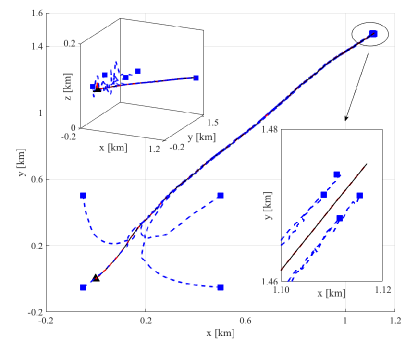
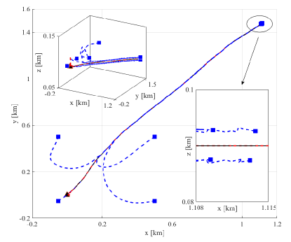
Figure 4: Simulated scenarios in LOS conditions with $4$ UAVs estimating ranging information (left) with an accuracy $\sigma_{\mathsf{r},0}=10^{-4}\,$m, and bearing information (right) with an accuracy $\sigma_{\mathsf{b},0}=10^{\circ}\,$deg. The initial positions and trajectory of the target and UAVs are indicated with black and blue lines, respectively. The estimated target trajectory is a dashed red line.

To solve the trajectory problem in (21), one can rely on an approach based on optimization theory (e.g., non-linear programming [45]) or on a more advanced approaches of machine learning (e.g., reinforcement learning algorithms [27], dynamic programming [46] or based on approaches based on graph neural networks [47]).

One possibility to solve the minimization problem in (21) is to use a numerical approach as, for example, the projection gradient method [45]

$$\mathbf{u}_{i}^{(k+1)}\!=\!-\nu\,\mathbf{P}\,\nabla_{\mathbf{p}_{i}^{(k)}}\,\mathcal{C}\left(\mathbf{J}_{i}^{(k)}\left(\hat{\mathbf{p}}_{0;i}^{(k)},\,\mathbf{L}_{i}^{(k)}\right)\right)\!-\!\mathbf{N}\left(\mathbf{N}^{\mathsf{T}}\mathbf{N}\right)^{-1}\mathbf{g},$$ (50)

where $\nu$ represents the spatial step, $\nabla_{\mathbf{p}_{i}^{(k)}}\,\left(\cdot\right)$ is the gradient operator with respect to the UAV positions which, taken with the negative sign, represents the direction of decrease of the cost function. The control signal computations are reported in Appendix C. The projection matrix is denoted with $\mathbf{P}=\mathbf{I}-\mathbf{N}\left(\mathbf{N}^{\mathsf{T}}\mathbf{N}\right)^{-1}\mathbf{N}^{\mathsf{T}}$ with $\mathbf{I}$ being the identity matrix and $\mathbf{N}=\left(\nabla_{\mathbf{p}_{i}^{(k)}}\mathbf{g}\right)$ being the gradient of the constraints in $\mathbf{g}=\left[\mathbf{g}_{1}\,\,\mathbf{g}_{2}\,\,\mathbf{g}_{3}\right]$, where

$$\mathbf{g}_{1}=\mathbf{d}_{\mathsf{U}}-d_{\mathsf{U}}^{*},\quad\mathbf{d}_{\mathsf{U}}=\left\{d_{ij}^{(k)}:d_{ij}^{(k)}<d_{\mathsf{U}}^{*}\right\},$$ (51)

$$\mathbf{g}_{2}=\mathbf{d}_{\mathsf{S}}-d_{\mathsf{T}}^{*},\,\,\,\,\,\,\mathbf{d}_{\mathsf{S}}=\left\{d_{i}^{(k)}:d_{i}^{(k)}<d_{\mathsf{T}}^{*}\right\},$$ (52)

$$\mathbf{g}_{3}=\mathbf{d}_{\mathsf{O}}-d_{\mathsf{O}}^{*},\,\,\,\,\,\mathbf{d}_{\mathsf{O}}=\left\{d_{i,\mathsf{O}}^{(k)}:d_{i,\mathsf{O}}^{(k)}<d_{\mathsf{O}}^{*}\right\}.$$ (53)

Finally, we limit the UAV speed, altitude and the maximum turning rates according to (27).

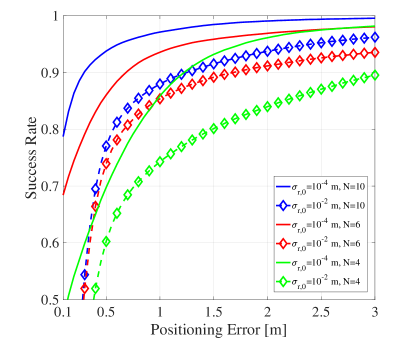
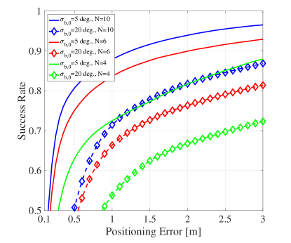
Figure 5: Success rate as a function of the number of UAVs for ranging (left) and bearing (right) measurements and different sensing accuracy.

VI Case Study

In this section, we analyze the performance of a DRN in different conditions: by changing the number of UAVs; by varying their sensing capabilities; by dealing with different RCS; by varying the number of communication hops; and by operating in LOS-NLOS channel conditions. The investigated scenarios are displayed in Figs. 4-9, with environments covering more than one square kilometer.

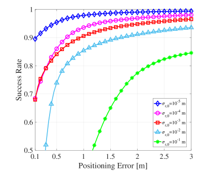
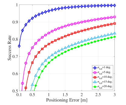
Figure 6: Success rate as a function of the ranging and bearing errors.

TABLE I: RMSE [m] on target position for the configurations of Fig.4

	$N=4$	$N=6$	$N=10$
Ranging-Only, $\sigma_{\mathsf{r},0}=10^{-4}$ m	0.53	0.33	0.15
Ranging-Only, $\sigma_{\mathsf{r},0}=10^{-2}$ m	1.55	0.82	0.64
Bearing-Only, $\sigma_{\mathsf{b},0}=5$ deg	1.38	0.85	0.82
Bearing-Only, $\sigma_{\mathsf{b},0}=20$ deg	3.85	2.27	1.55

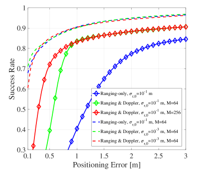
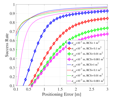
Figure 7: Success rate as a function of the positioning error when ranging measurements are collected. On the left, the case with and without Doppler shifts is considered for a ranging error of $\sigma_{\mathsf{r},0}=10^{-3}\,$m (dashed lines) and $\sigma_{\mathsf{r},0}=10^{-1}\,$m (diamond markers); on the right, the performance is compared as a function of the RCS.

In the simulations, the target mobility in (19) was modeled according to a random walk model [35], with

$$\mathbf{A}\!=\!\left[\begin{array}[]{cc}\mathbf{I}_{3\times 3}&\Delta t\,\mathbf{I}_{3\times 3}\\ \mathbf{0}_{3\times 3}&\mathbf{I}_{3\times 3}\end{array}\right],\mathbf{Q}\!=\!\left[\begin{array}[]{cc}\frac{\Delta t^{3}}{3}\,\mathbf{W}&\frac{\Delta t^{2}}{2}\,\mathbf{W}\\ \frac{\Delta t^{2}}{2}\,\mathbf{W}&\Delta t\,\mathbf{W}\end{array}\right],$$ (58)

where $\mathbf{W}=\text{diag}\left(w_{\mathsf{x}},\,w_{\mathsf{y}},\,w_{\mathsf{z}}\right)=\left(10^{-5},\,10^{-5},\,0\right)$ is a diagonal matrix containing the variances of the process noise in each direction. The number of UAVs and the target RCS were set to $6$ and $0.1\,$m², if not otherwise indicated. The safety distances, i.e., $d_{\mathsf{U}}^{*}$, $d_{\mathsf{T}}^{*}$ and $d_{\mathsf{O}}^{*}$, were all fixed at $5\,$m, the number of Monte Carlo iterations and the trajectory time steps at $100$ and $3000$ (each time step lasts 1 second), respectively. A communication range of $900$ m between the UAVs and a single hop were considered [27, 48], if not otherwise indicated. We initialized the EKF as $\mathbf{m}_{i}^{(0)}=\mathbf{0}_{6\times 1}$ and $\mathbf{P}_{i}^{(0)}=\text{diag}\left(20^{2}\cdot\mathbf{I}_{3\times 3},\,0.5^{2}\cdot\mathbf{I}_{3\times 3}\right)$.

To compare the results, the success rate was evaluated as

$$\mathsf{SR}\left(e_{\mathsf{th}}\right)=\frac{1}{K\,N_{\mathsf{MC}}\,N}\sum_{k=1}^{K}\,\sum_{i=1}^{N}\sum_{m=1}^{N_{\mathsf{MC}}}\mathbf{1}\left(e_{\mathsf{th}}-e_{im}^{(k)}\right),$$ (59)

where $N_{\mathsf{MC}}$ is the number of Monte Carlo iterations, $K$ is the number of time steps, $\mathbf{1}\left(x\right)$ is the unit step function that is equal to $1$ if $x\geq 0$ and $0$ otherwise, $e_{im}^{(k)}$ is the estimation error of the target position at the $i$-th UAV for the $m$-th Monte Carlo iteration, where $e_{i,m}^{(k)}=\lVert\hat{\mathbf{p}}_{0;im}^{(k)}-\mathbf{p}_{0}^{(k)}\rVert_{2}$, and $e_{\mathsf{th}}$ is a localization threshold.

In the simulations of Fig. 4, the initial positions of UAVs were at the vertexes of a square lying on the $XY$-plane with $x_{i}^{(0)}=\left[-50,\,-50,\,500,\,500\right]^{\mathsf{T}}\,$m, $y_{i}^{(0)}=\left[-50,\,500,\,-50,\,500\right]^{\mathsf{T}}\,$m, and $z_{i}^{(0)}\sim\mathcal{U}\left[80,150\right]\,$m, while the target initial position and velocity were $\left[0,0,90\right]^{\mathsf{T}}\,$m and $\left[-0.3,0.4,0\right]^{\mathsf{T}}\,$m/s.

In Fig. 4, we present qualitative examples of estimated UAV trajectories for different sensing capabilities (ranging and bearing) and considering $N=4$. The trajectories of UAVs are reported as blue lines and the positions are displayed with blue square markers for the initial and last time instants. The initial target position is drawn with a black triangle and its actual trajectory with a continuous black line. The estimated trajectory of the target is marked with a red dotted line. As can be seen, after an initial transient, the UAVs of the DRN jointly surround the target.

Given this scenario, in Table I, we show the tracking performance in terms of average root mean squared error (RMSE) by varying the measurement accuracy and considering different number of UAVs. The RMSE on position and velocity was averaged over the number of discrete time instants and over the number of UAVs. A group of four radars with only ranging capability and accuracy of $\sigma_{\mathsf{r},0}=10^{-2}\,$m obtains approximately the same tracking performance of four radars with only bearing capability and accuracy of about $5^{\circ}\,$degrees. Instead, when considering a better performing radar, such as the FMCW radar in [49] (i.e., with $\sigma_{\mathsf{r},0}\approx 10^{-4}\,$m), the average localization accuracy is below $1\,$m.

In Fig. 5, we provide the success rate evaluated as in (59) by varying the number of UAVs and the sensing capabilities. A localization error lower than $1\,$m can be achieved in nearly $80\%$ of the cases with $N=4$ drones with either a reference ranging accuracy of $10^{-2}\,$m or a bearing accuracy of $5^{\circ}\,$degrees. This is also confirmed by Fig. 6 where several ranging and bearing errors were tested.

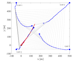
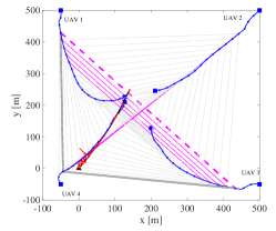
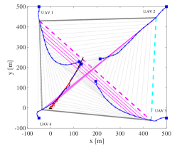
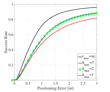
Figure 8: Plot of the first $K=500$ instants of the trajectories with highlighted multi-hop connections. Top (from the left to the right): Single-hop scenario ($h_{\mathsf{max}}=1$); double-hop scenario ($h_{\mathsf{max}}=2$) with links reported with grey and magenta lines when a 1- or 2-hop is established, respectively; and triple-hop scenario ($h_{\mathsf{max}}=3$) with links reported with grey, magenta and cyan lines when a 1- or 2- or 3-hop is established, respectively. Bottom: Success rate as a function of the maximum number of hops.

We now investigate the impact of the Doppler shifts and target RCS on the tracking performance with a fixed number of UAVs ($N=6$). In Fig. 7-left, we show the success rate by considering ranging measurements and the presence of Doppler shifts with different chirp gains (i.e., $M_{i}=64$-$256$) and different ranging accuracies. It can be observed that relying on Doppler shifts in addition to ranging measurements is beneficial especially when ranging is not sufficiently accurate: by fixing the desired localization error to $1\,$meter, the percentage increase experienced by adding Doppler shifts in the measurement vector is approximately of $100\%$ with a ranging error of $\sigma_{\mathsf{r},0}=10^{-1}\,$m (with $M_{i}=256,\,\,\,\forall i=1,\ldots,N$) whereas there are no evident improvements for $\sigma_{\mathsf{r},0}=10^{-3}\,$m. Finally, in Fig. 7-right, we plot the success rate as a function of the target RCS. It is interesting to notice that a UAV with a RCS of $0.01\,$m can be localized in the $90\%$ of cases with an error lower than $1$ meter provided that a sensor with a ranging accuracy of $10^{-3}\,$m is adopted.

In Fig. 8, we study the impact of a multi-hop exchange of measurements by limiting the number of temporal steps to $K=500$ because the impact of multi-hops is more evident at the beginning of the trajectory. The ranging accuracy was $\sigma_{\mathsf{r},0}=10^{-3}\,$m, the number of UAVs to $N=4$, and a communication range of $r_{\mathsf{max}}=505\,$m was considered. In Fig. 8, from the left to the right, we have plotted the single hop scenario with links depicted with grey lines, the two-hop schenario, i.e., $h_{\mathsf{max}}=2$, with magenta lines and $3-$hop case with cyan lines, respectively. For example, in the single hop case, UAV 1 is only connected with UAV 4 at time instant $k=30$ because $h_{\mathsf{max}}=1$ and by having $r_{\mathsf{max}}=505\,$m only UAV 4 is in the neighboring set of UAV 1. Contrarily, when $h_{\mathsf{max}}=2$, it is also connected with UAV 3 through UAV 4. This means that the ranging information collected by UAV 3 will be available at UAV 1 after two time instants. Apart from an initial transient when the multi-hop propagation can be helpful as it allows to connect nodes otherwise unreachable, for the majority of the navigation time, a single-hop is sufficient thanks to the fact that the navigation control is conceived for minimizing the tracking error and, consequently, for minimizing the UAV-target and inter-UAVs distances. This is also confirmed from the results plotted in Fig. 8-(bottom) in terms of success rate.

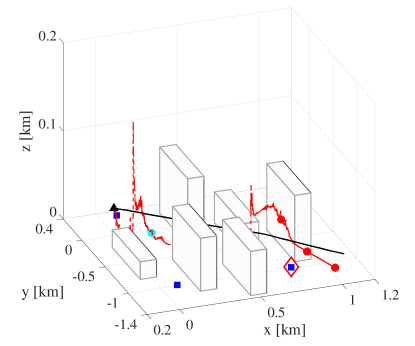
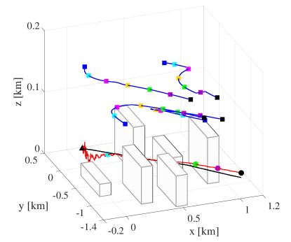
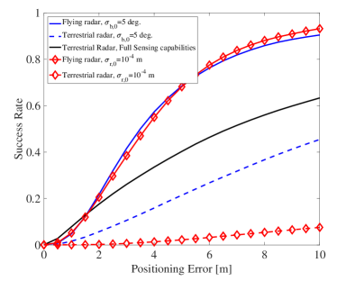
Figure 9: Simulated scenarios in NLOS conditions and success rate as a function of radar network configuration: comparison between terrestrial/fixed and flying/dynamic radars, and success rate results (bottom).

TABLE II: RMSE for the configurations of Fig.9

	RMSE on position [m]		RMSE on velocity [m/s]
	Terr. Rad.	Flying Rad.	Terr. Rad.	Flying Rad.
Ranging-Only	65.17	5.07	0.12	0.05
Bearing-Only	17.43	5.70	0.071	0.063

At this point, we aim at comparing the performance of a DRN in presence of obstacles in order to assess the advantages of DRNs with respect to terrestrial fixed radar networks. To this purpose, we consider the scenario of Fig. 9 where obstacles are depicted with grey parallelepipeds, the UAVs composing the DRN with squared markers of different colors (every $500$ time steps), and the terrestrial radars with squared blue markers. The ranging and bearing errors were $10^{-4}\,$m and $5^{\circ}\,$degrees, respectively. In the DRN, the UAV initial positions were $x_{i}^{(0)}=\left[100,\,100,\,800,\,800\right]^{\mathsf{T}}\,$m, $y_{i}^{(0)}=\left[-1000,\,300,\,300,\,-1000\right]^{\mathsf{T}}\,$m, and with a UAV height $z_{i}^{(0)}\sim\mathcal{U}\left[90,150\right]\,$m. The target altitude was set to $30\,$m, and its trajectory followed the dynamics described by (58). For a better comparison, two situations with a fixed deployment of radar sensors were considered: one with a single terrestrial radar with full sensing capabilities (capable of retrieving ranging, bearing and Doppler shift information) represented with a red diamond in Fig. 9-top, and another where, for fairness of comparison, the fixed radar network is with the same number ($N=4$) and sensing capabilities of UAVs. These radar configurations are compared in Fig. 9-bottom showing the superiority of a dynamic radar configuration over terrestrial networks in terms of success rate. Moreover, the RMSE results on position and velocity are reported in Table II. In the case of a single terrestrial radar with full sensing capabilities, the RMSE on position and velocities is of $11.36\,$m and $0.06\,$m/s, respectively.

VII Conclusion

In this paper, the idea of a UAV dynamic radar network for the tracking of a non-cooperative (e.g., unauthorized) UAV has been described. In contrast with current on-ground radar systems, the UAV network provides new degrees of freedom thanks to its reconfigurability and flexibility. Moreover, the UAVs are considered autonomous in navigating and estimating their best trajectory to minimize the tracking error of the dynamic target. The proposed network has heterogeneous sensing capabilities and estimates are shared among the UAVs. In this sense, the UAV cooperation can significantly increase the tracking accuracy without impacting the communication latency. The proposed control law aimed at minimizing an information-driven cost function derived starting from measurements and estimates exchanged by the UAVs at each time instant.

Results demonstrate that having a flexible network instead of a terrestrial deployment of radars helps in preventing NLOS conditions and, thus, in better tracking a non-cooperative target. Moreover, even if the intruder is a small UAV (a target with RCS of $0.1\,$m² or less), the positioning performance is below $1\,$m most of the time, provided that a radar sensor with a millimeter ranging accuracy is available on-board, as for example a FMCW radar operating at $77\,$GHz. The same performance can be obtained with bearing measurements given an angular accuracy of about $5^{\circ}\,$degrees. Finally the use of Doppler shift estimates is beneficial to retrieve the velocity of the target instead of inferring it from position estimates. For this reason, the impact of the Doppler shift estimates is more valuable in the case where the ranging error is larger. Future directions of research include the development of a control law able to maximize the expected information metric over a longer horizon (non-myopic approach) in order to deal better with complex and dynamic environments.

Appendix A

The elements in (49) provide the geometric matrix relative to Doppler shift measurements, and they are given by

$$\mathbf{G}_{\mathsf{d},j}^{(\ell_{k})}\left(\mathbf{p}_{0}^{(k)},\mathbf{p}_{j}^{(\ell_{k})}\right) =\left[\nabla_{\mathbf{p}_{0}^{(k)}}^{\mathsf{T}}\left(f_{\mathsf{d},j}^{(\ell_{k})}\right)\,\nabla_{\mathbf{p}_{0}^{(k)}}\left(f_{\mathsf{d},j}^{(\ell_{k})}\right)\right]_{\mathbf{s}^{(k)}=\mathbf{s}_{0}^{-}}=\left(\frac{\gamma}{2\,\lambda}\right)^{2}\,\left[\begin{array}[]{ccc}g_{\mathsf{xx}}&g_{\mathsf{xy}}&g_{\mathsf{xz}}\\ g_{\mathsf{xy}}&g_{\mathsf{yy}}&g_{\mathsf{yz}}\\ g_{\mathsf{xz}}&g_{\mathsf{yz}}&g_{\mathsf{zz}}\\ \end{array}\right],$$ (63)

with $\mathbf{s}_{0}^{-}=\hat{\mathbf{s}}_{i}^{(k\lvert k-1)}$ and

$$g_{\mathsf{xx}}\!=\!\left(-\mathsf{s}_{\phi,j}^{(\ell_{k})}\,\mathsf{s}_{\theta,j}^{(\ell_{k})}\,\omega_{\mathsf{z}}+\mathsf{c}_{\theta,j}^{(\ell_{k})}\,\omega_{\mathsf{y}}\right)^{2},$$

$$g_{\mathsf{yy}}\!=\!\left(\mathsf{c}_{\phi,j}^{(\ell_{k})}\,\mathsf{s}_{\theta,j}^{(\ell_{k})}\,\omega_{\mathsf{z}}{-}\mathsf{c}_{\theta,j}^{(\ell_{k})}\,\omega_{\mathsf{x}}\right)^{2},$$

$$g_{\mathsf{zz}}\!=\!\left(-\mathsf{c}_{\phi,j}^{(\ell_{k})}\,\mathsf{s}_{\theta,j}^{(\ell_{k})}\,\omega_{\mathsf{y}}+\mathsf{s}_{\phi,j}^{(\ell_{k})}\,\mathsf{s}_{\theta,j}^{(\ell_{k})}\,\omega_{\mathsf{x}}\right)^{2},$$

$$g_{\mathsf{xy}}\!=\!\left(-\mathsf{s}_{\phi,j}^{(\ell_{k})}\,\mathsf{s}_{\theta,j}^{(\ell_{k})}\,\omega_{\mathsf{z}}+\mathsf{c}_{\theta,j}^{(\ell_{k})}\,\omega_{\mathsf{y}}\right)\!\left(\mathsf{c}_{\phi,j}^{(\ell_{k})}\,\mathsf{s}_{\theta,j}^{(\ell_{k})}\,\omega_{\mathsf{z}}{-}\mathsf{c}_{\theta,j}^{(\ell_{k})}\,\omega_{\mathsf{x}}\right),$$

$$g_{\mathsf{xz}}\!=\!\left(\mathsf{s}_{\phi,j}^{(\ell_{k})}\mathsf{s}_{\theta,j}^{(\ell_{k})}\omega_{\mathsf{z}}-\mathsf{c}_{\theta,j}^{(\ell_{k})}\omega_{\mathsf{y}}\right)\!\left(\mathsf{c}_{\phi,j}^{(\ell_{k})}\mathsf{s}_{\theta,j}^{(\ell_{k})}\omega_{\mathsf{y}}-\mathsf{s}_{\phi,j}^{(\ell_{k})}\mathsf{s}_{\theta,j}^{(\ell_{k})}\omega_{\mathsf{x}}\right),$$

$$g_{\mathsf{yz}}\!=\!\left(\mathsf{c}_{\phi,j}^{(\ell_{k})}\mathsf{s}_{\theta,j}^{(\ell_{k})}\omega_{\mathsf{z}}{-}\mathsf{c}_{\theta,j}^{(\ell_{k})}\omega_{\mathsf{x}}\right)\!\left(-\mathsf{c}_{\phi,j}^{(\ell_{k})}\mathsf{s}_{\theta,j}^{(\ell_{k})}\omega_{y}+\mathsf{s}_{\phi,j}^{(\ell_{k})}\mathsf{s}_{\theta,j}^{(\ell_{k})}\,\omega_{\mathsf{x}}\right).$$

Appendix B

In this appendix, the elements of the information matrix in (44), that is,

$$\mathbf{J}_{i}^{(k)}\left(\mathbf{p}_{0}^{(k)};\mathbf{L}_{i}^{(k)}\right) =\left[\begin{array}[]{ccc}J_{\mathsf{xx},i}&J_{\mathsf{xy},i}&J_{\mathsf{xz},i}\\ J_{\mathsf{xy},i}&J_{\mathsf{yy},i}&J_{\mathsf{yz},i}\\ J_{\mathsf{xz},i}&J_{\mathsf{yz},i}&J_{\mathsf{zz},i}\\ \end{array}\right],$$ (67)

are expanded in scalar notation. In particular, we have

$$J_{\mathsf{xx},i} =J_{\mathsf{xx},i}^{-}\!+\!\sum_{j=1}^{\lvert\mathcal{N}_{\mathsf{nb},i}^{(k)}\rvert}\!\mathrm{l}_{j}^{(\ell_{k})}\,\left\{\frac{\kappa_{j}\,\gamma^{2}}{4\,\left(\sigma_{\mathsf{r},j}^{(\ell_{k})}\right)^{2}}\,\left(\mathsf{c}_{\phi,j}^{(\ell_{k})}\mathsf{s}_{\theta,j}^{(\ell_{k})}\right)^{2}+\frac{\beta_{j}}{\left(\sigma_{\mathsf{b},j}^{(\ell_{k})}\,d_{j}^{(\ell_{k})}\right)^{2}}\,\left[\left(\frac{\mathsf{s}_{\phi,j}^{(\ell_{k})}}{\mathsf{s}_{\theta,j}^{(\ell_{k})}}\right)^{2}+\left(\mathsf{c}_{\phi,j}^{(\ell_{k})}\,\mathsf{c}_{\theta,j}^{(\ell_{k})}\right)^{2}\right]\right.$$

$$\left.+\frac{\xi_{j}\,\gamma^{2}\,}{4\,\lambda^{2}\,\left(\sigma_{\mathsf{d},j}^{(\ell_{k})}\right)^{2}}\,g_{\mathsf{xx}}\right\},$$ (68)

$$J_{\mathsf{xy},i} =\,J_{\mathsf{xy},i}^{-}+\sum_{j=1}^{\lvert\mathcal{N}_{\mathsf{nb},i}^{(k)}\rvert}\mathrm{l}_{j}^{(\ell_{k})}\left\{\frac{\kappa_{j}\,\gamma^{2}}{4\,\left(\sigma_{\mathsf{r},j}^{(\ell_{k})}\right)^{2}}\,\mathsf{s}_{\phi,j}^{(\ell_{k})}\,\mathsf{c}_{\phi,j}^{(\ell_{k})}\,\left(\mathsf{s}_{\theta,j}^{(\ell_{k})}\right)^{2}+\xi_{j}\,\frac{\gamma^{2}\,g_{\mathsf{xy}}}{4\,\lambda^{2}\,\left(\sigma_{\mathsf{d},j}^{(\ell_{k})}\right)^{2}}-\frac{\beta_{j}}{\left(\sigma_{\mathsf{b},j}^{(\ell_{k})}\,d_{j}^{(\ell_{k})}\right)^{2}}\frac{\mathsf{s}_{\phi,j}^{(\ell_{k})}\,\mathsf{c}_{\phi,j}^{(\ell_{k})}}{\left(\mathsf{s}_{\theta,j}^{(\ell_{k})}\right)^{2}}\right.$$

$$\left.+\frac{\beta_{j}}{\left(\sigma_{\mathsf{b},j}^{(\ell_{k})}\,d_{j}^{(\ell_{k})}\right)^{2}}\mathsf{s}_{\phi,j}^{(\ell_{k})}\,\mathsf{c}_{\phi,j}^{(\ell_{k})}\,\left(\mathsf{c}_{\theta,j}^{(\ell_{k})}\right)^{2}\right\},$$ (69)

$$J_{\mathsf{xz},i} =\,J_{\mathsf{xz},i}^{-}+\sum_{j=1}^{\lvert\mathcal{N}_{\mathsf{nb},i}^{(k)}\rvert}\,\mathrm{l}_{j}^{(\ell_{k})}\,\left\{\frac{\kappa_{j}\,\gamma^{2}}{4\,\left(\sigma_{\mathsf{r},j}^{(\ell_{k})}\right)^{2}}\,\mathsf{c}_{\phi,j}^{(\ell_{k})}\,\mathsf{s}_{\theta,j}^{(\ell_{k})}\,\mathsf{c}_{\theta,j}^{(\ell_{k})}-\frac{\beta_{j}}{\left(\sigma_{\mathsf{b},j}^{(\ell_{k})}\,d_{j}^{(\ell_{k})}\right)^{2}}\,\mathsf{c}_{\phi,j}^{(\ell_{k})}\,\mathsf{s}_{\theta,j}^{(\ell_{k})}\,\mathsf{c}_{\theta,j}^{(\ell_{k})}+\frac{\xi_{j}\,\gamma^{2}}{{2}\,\lambda^{2}\,\left(\sigma_{\mathsf{d},j}^{(\ell_{k})}\right)^{2}}\,g_{\mathsf{xz}}\right\},$$ (70)

$$J_{\mathsf{yy},i} =J_{\mathsf{yy},i}^{-}+\sum_{j=1}^{\lvert\mathcal{N}_{\mathsf{nb},i}^{(k)}\rvert}\mathrm{l}_{j}^{(\ell_{k})}\,\left\{\frac{\kappa_{j}\,\gamma^{2}}{4\,\left(\sigma_{\mathsf{r},j}^{(\ell_{k})}\right)^{2}}\,\left(\mathsf{s}_{\phi,j}^{(\ell_{k})}\,\mathsf{s}_{\theta,j}^{(\ell_{k})}\right)^{2}+\frac{\beta_{j}}{\left(\sigma_{\mathsf{b},j}^{(\ell_{k})}\,d_{j}^{(\ell_{k})}\right)^{2}}\left[\left(\frac{\mathsf{c}_{\phi,j}^{(\ell_{k})}}{\mathsf{s}_{\theta,j}^{(\ell_{k})}}\right)^{2}+\left(\mathsf{s}_{\phi,j}^{(\ell_{k})}\,\mathsf{c}_{\theta,j}^{(\ell_{k})}\right)^{2}\right]\right.$$

$$\left.+\xi_{j}\,\frac{\gamma^{2}}{4\,\lambda^{2}\,\left(\sigma_{\mathsf{d},j}^{(\ell_{k})}\right)^{2}}\,\,g_{\mathsf{yy}}\right\},$$ (71)

$$J_{\mathsf{zz},i} =\,J_{\mathsf{zz},i}^{-}+\sum_{j=1}^{\lvert\mathcal{N}_{\mathsf{nb},i}^{(k)}\rvert}\mathrm{l}_{j}^{(\ell_{k})}\left\{\frac{\kappa_{j}\,\gamma^{2}}{4\,\left(\sigma_{\mathsf{r},j}^{(\ell_{k})}\right)^{2}}\,\left(\mathsf{c}_{\theta,j}^{(\ell_{k})}\right)^{2}+\frac{\xi_{j}\,\gamma^{2}}{4\,\lambda^{2}\,\left(\sigma_{\mathsf{d},j}^{(\ell_{k})}\right)^{2}}\,g_{\mathsf{zz}}+\beta_{j}\,\frac{1}{\left(\sigma_{\mathsf{b},j}^{(\ell_{k})}d_{j}^{(\ell_{k})}\right)^{2}}\,\left(\mathsf{s}_{\theta,j}^{(\ell_{k})}\right)^{2}\right\},$$ (72)

$$J_{\mathsf{yz},i} =\,\,J_{\mathsf{yz},i}^{-}+\sum_{j=1}^{\lvert\mathcal{N}_{\mathsf{nb},i}^{(k)}\rvert}\mathrm{l}_{j}^{(\ell_{k})}\left\{\frac{\kappa_{j}\,\gamma^{2}}{4\,\left(\sigma_{\mathsf{r},j}^{(\ell_{k})}\right)^{2}}\,\mathsf{s}_{\theta,j}^{(\ell_{k})}\,\mathsf{c}_{\theta,j}^{(\ell_{k})}\,\mathsf{s}_{\phi,j}^{(\ell_{k})}+\frac{\xi_{j}\,\gamma^{2}}{4\,\lambda^{2}\,\left(\sigma_{\mathsf{d},j}^{(\ell_{k})}\right)^{2}}\,g_{\mathsf{yz}}\,-\,\frac{\beta_{j}}{\left(\sigma_{\mathsf{b},j}^{(\ell_{k})}\,d_{j}^{(\ell_{k})}\right)^{2}}\,\mathsf{s}_{\phi,j}^{(\ell_{k})}\,\mathsf{s}_{\theta,j}^{(\ell_{k})}\,\mathsf{c}_{\theta,j}^{(\ell_{k})}\right\}.$$ (73)

Appendix C

In this appendix, we derive the analytical expressions for control signals in (50). More specifically, we determine the term $\nabla_{\mathbf{p}_{i}^{(k)}}\,\mathcal{C}\left(\hat{\mathbf{p}}_{0;i}^{(k)},\mathbf{L}_{i}^{(k)}\right)$. According to (22), we have

$$\nabla_{\mathbf{p}_{i}^{(k)}}\,\mathcal{C}\left(\hat{\mathbf{p}}_{0;i}^{(k)},\mathbf{L}_{i}^{(k)}\right) =-\frac{\nabla_{\mathbf{p}_{i}^{(k)}}\left(\mathcal{D}_{i}^{(k)}\left(\mathbf{L}_{i}^{(k)}\right)\right)}{\mathcal{D}_{i}^{(k)}\left(\mathbf{L}_{i}^{(k)}\right)},$$ (74)

where $\mathcal{D}_{i}^{(k)}\left(\mathbf{L}_{i}^{(k)}\right)=\det\left(\mathbf{J}_{i}^{(k)}\left(\hat{\mathbf{p}}_{0;i}^{(k)};\mathbf{L}_{i}^{(k)}\right)\right)=J_{\mathsf{xx},i}\,C_{\mathsf{xx}}+J_{\mathsf{xy},i}\,C_{\mathsf{yx}}+J_{\mathsf{xz},i}\,C_{\mathsf{zx}}$ is the determinant of the information matrix, and $C_{\mathsf{xx}}=J_{\mathsf{yy},i}J_{\mathsf{zz},i}-J_{\mathsf{zy},i}^{2}$ $C_{\mathsf{xy}}=C_{\mathsf{yx}}=J_{\mathsf{xz},i}J_{\mathsf{zy},i}-J_{\mathsf{xy},i}\,J_{\mathsf{zz},i}$, $C_{\mathsf{xz}}=C_{\mathsf{zx}}=J_{\mathsf{xy},i}J_{\mathsf{yz},i}-J_{\mathsf{xz},i}\,J_{\mathsf{yy},i}$, $C_{\mathsf{yy}}=J_{\mathsf{xx},i}\,J_{\mathsf{zz},i}-J_{\mathsf{xz},i}^{2}$, $C_{\mathsf{yz}}=J_{\mathsf{xz},i}\,J_{\mathsf{yx},i}-J_{\mathsf{xx},i}\,J_{\mathsf{yz},i}$, $C_{\mathsf{zz}}=J_{\mathsf{xx},i}\,J_{\mathsf{yy},i}-J_{\mathsf{xy},i}^{2}$ are the cofactors of the inverse. Consequently, the derivatives of the cost functions are

$$\nabla_{\mathbf{p}_{i}^{(k)}}\left(\mathcal{D}_{i}^{(k)}\left(\mathbf{L}_{i}^{(k)}\right)\right) =\left(\nabla_{\mathbf{p}_{i}^{(k)}}J_{\mathsf{xx},i}\right)C_{\mathsf{xx}}+\left(\nabla_{\mathbf{p}_{i}^{(k)}}C_{\mathsf{xx}}\right)J_{\mathsf{xx},i}+\left(\nabla_{\mathbf{p}_{i}^{(k)}}J_{\mathsf{xy},i}\right)C_{\mathsf{yx}}+\left(\nabla_{\mathbf{p}_{i}^{(k)}}C_{\mathsf{yx}}\right)J_{\mathsf{xy},i}$$

$$+\left(\nabla_{\mathbf{p}_{i}^{(k)}}J_{\mathsf{xz},i}\right)C_{\mathsf{zx}}+\left(\nabla_{\mathbf{p}_{i}^{(k)}}C_{\mathsf{xz}}\right)J_{\mathsf{zx},i}\,,$$ (75)

where

$$\nabla_{\mathbf{p}_{i}^{(k)}}C_{\mathsf{xx}} =\left(\nabla_{\mathbf{p}_{i}^{(k)}}J_{\mathsf{yy},i}\right)J_{\mathsf{zz},i}+\left(\nabla_{\mathbf{p}_{i}^{(k)}}J_{\mathsf{zz},i}\right)J_{\mathsf{yy},i}-2\,J_{\mathsf{zy},i}\,\left(\nabla_{\mathbf{p}_{i}^{(k)}}J_{\mathsf{zy},i}\right),$$

$$\nabla_{\mathbf{p}_{i}^{(k)}}C_{\mathsf{yx}} =\left(\nabla_{\mathbf{p}_{i}^{(k)}}J_{\mathsf{xz},i}\right)J_{\mathsf{zy},i}+J_{\mathsf{xz},i}\left(\nabla_{\mathbf{p}_{i}^{(k)}}J_{\mathsf{zy},i}\right)-\left(\nabla_{\mathbf{p}_{i}^{(k)}}J_{\mathsf{xy},i}\right)\,J_{\mathsf{zz},i}-J_{\mathsf{xy},i}\,\left(\nabla_{\mathbf{p}_{i}^{(k)}}J_{\mathsf{zz},i}\right),$$

$$\nabla_{\mathbf{p}_{i}^{(k)}}C_{\mathsf{xz}} =\left(\nabla_{\mathbf{p}_{i}^{(k)}}J_{\mathsf{xy},i}\right)J_{\mathsf{yz},i}+J_{\mathsf{xy},i}\left(\nabla_{\mathbf{p}_{i}^{(k)}}J_{\mathsf{yz},i}\right)-\left(\nabla_{\mathbf{p}_{i}^{(k)}}J_{\mathsf{xz},i}\right)\,J_{\mathsf{yy},i}-J_{\mathsf{xz},i}\,\left(\nabla_{\mathbf{p}_{i}^{(k)}}J_{\mathsf{yy},i}\right).$$ (76)

Starting from (73), it is straightforward to derive (76).

References

- [1] N. Zhao et al., “UAV-assisted emergency networks in disasters,” IEEE Wireless Commun., vol. 26, no. 1, pp. 45–51, 2019.
- [2] R. Shakeri et al., “Design challenges of multi-UAV systems in cyber-physical applications: A comprehensive survey, and future directions,” IEEE Commun. Surveys & Tutorials, 2019.
- [3] M. Mozaffari, A. T. Z. Kasgari, W. Saad, M. Bennis, and M. Debbah, “Beyond 5G with UAVs: Foundations of a 3D wireless cellular network,” IEEE Trans. Wireless Commun., vol. 18, no. 1, pp. 357–372, 2018.
- [4] R. Gangula, P. de Kerret, O. Esrafilian, and D. Gesbert, “Trajectory optimization for mobile access point,” in Proc. 2017 51st Asilomar Conf. Signals, Sys., Comput. IEEE, 2017, pp. 1412–1416.
- [5] J. Chen, U. Yatnalli, and D. Gesbert, “Learning radio maps for UAV-aided wireless networks: A segmented regression approach,” in Proc. 2017 IEEE Int. Conf. Commun. (ICC). IEEE, 2017, pp. 1–6.
- [6] P. Cerwall, P. Jonsson, R. Möller, S. Bävertoft, S. Carson, and I. Godor, “Ericsson mobility report,” On the Pulse of the Networked Society. Hg. v. Ericsson, 2015.
- [7] I. Guvenc, F. Koohifar, S. Singh, M. L. Sichitiu, and D. Matolak, “Detection, tracking, and interdiction for amateur drones,” IEEE Commun. Mag., vol. 56, no. 4, pp. 75–81, 2018.
- [8] F. Koohifar, I. Guvenc, and M. L. Sichitiu, “Autonomous tracking of intermittent RF source using a UAV swarm,” IEEE Access, vol. 6, pp. 15 884–15 897, 2018.
- [9] I. Bisio, C. Garibotto, F. Lavagetto, A. Sciarrone, and S. Zappatore, “Unauthorized amateur UAV detection based on WiFi statistical fingerprint analysis,” IEEE Commun. Mag., vol. 56, no. 4, pp. 106–111, 2018.
- [10] P. Hügler, F. Roos, M. Schartel, M. Geiger, and C. Waldschmidt, “Radar taking off: New capabilities for UAVs,” IEEE Microw. Mag., vol. 19, no. 7, pp. 43–53, 2018.
- [11] M. Ezuma, O. Ozdemir, C. K. Anjinappa, W. A. Gulzar, and I. Guvenc, “Micro-UAV detection with a low-grazing angle millimeter wave radar,” arXiv preprint arXiv:1902.05483, 2019.
- [12] D. Casbeer, A. L. Swindlehurst, and R. Beard, “Connectivity in a UAV multi-static radar network,” in AIAA Guidance, Navig., Control Conf. Exhibit, 2006, p. 6209.
- [13] D. Solomitckii, M. Gapeyenko, V. Semkin, S. Andreev, and Y. Koucheryavy, “Technologies for efficient amateur drone detection in 5G millimeter-wave cellular infrastructure,” IEEE Commun. Mag., vol. 56, no. 1, pp. 43–50, 2018.
- [14] B. Paul and D. W. Bliss, “Extending joint radar-communications bounds for FMCW radar with doppler estimation,” in Proc. 2015 IEEE Radar Conf. (RadarCon). IEEE, 2015, pp. 0089–0094.
- [15] S. Schuster, S. Scheiblhofer, L. Reindl, and A. Stelzer, “Performance evaluation of algorithms for SAW-based temperature measurement,” IEEE Trans. Ultrason. Ferroelectr. Freq. Control, vol. 53, no. 6, pp. 1177–1185, 2006.
- [16] Y. Liu, W. Li, Q. Lu, J. Wang, and Y. Shen, “Relative localization of ground vehicles using non-terrestrial networks,” in 2019 IEEE/CIC Int. Conf. Commun. Workshops China (ICCC Workshops). IEEE, 2019, pp. 93–97.
- [17] A. Guerra, N. Sparnacci, D. Dardari, and P. M. Djurić, “Collaborative target-localization and information-based control in networks of UAVs,” in Proc. 2018 IEEE 19th Inter. Workshop Signal Process. Adv. Wireless Commun. (SPAWC). IEEE, 2018, pp. 1–5.
- [18] A. Guerra, D. Dardari, and P. M. Djurić, “Joint indoor localization and navigation of uavs for network formation control,” in Proc. 2018 52nd Asilomar Conf. Signals, Sys., Comput. IEEE, 2018, pp. 13–19.
- [19] A. Guerra, D. Dardari, and P. M. Djuric, “Non-centralized navigation for source localization by cooperative uavs,” arXiv preprint arXiv:1910.12780, 2019.
- [20] R. Feger, C. Wagner, S. Schuster, S. Scheiblhofer, H. Jager, and A. Stelzer, “A 77-GHz FMCW MIMO radar based on an SiGe single-chip transceiver,” IEEE Trans. Microw. Theory and Techn., vol. 57, no. 5, pp. 1020–1035, 2009.
- [21] F. Folster, H. Rohling, and U. Lubbert, “An automotive radar network based on 77 GHz FMCW sensors,” in Proc. IEEE Int. Radar Conf., 2005. IEEE, 2005, pp. 871–876.
- [22] F. Hoffmann, M. Ritchie, F. Fioranelli, A. Charlish, and H. Griffiths, “Micro-doppler based detection and tracking of UAVs with multistatic radar,” in Proc. 2016 IEEE Radar Conf. (RadarConf). IEEE, 2016, pp. 1–6.
- [23] S. Martínez and F. Bullo, “Optimal sensor placement and motion coordination for target tracking,” Automatica, vol. 42, no. 4, pp. 661–668, 2006.
- [24] S. Ragi and E. K. Chong, “UAV path planning in a dynamic environment via partially observable Markov decision process,” IEEE Trans. Aerosp. Electron. Syst., vol. 49, no. 4, pp. 2397–2412, 2013.
- [25] Z. M. Kassas and T. E. Humphreys, “Receding horizon trajectory optimization in opportunistic navigation environments,” IEEE Trans. Aerosp. Electron. Syst., vol. 51, no. 2, pp. 866–877, 2015.
- [26] K. Dogancay, “UAV path planning for passive emitter localization,” IEEE Trans. Aerosp. Electron. Syst., vol. 48, no. 2, pp. 1150–1166, 2012.
- [27] C. Wang, J. Wang, Y. Shen, and X. Zhang, “Autonomous navigation of UAVs in large-scale complex environments: A deep reinforcement learning approach,” IEEE Trans. Veh. Technol., vol. 68, no. 3, pp. 2124–2136, 2019.
- [28] Y. Cai and Y. Shen, “An integrated localization and control framework for multi-agent formation,” IEEE Trans. Signal Process., vol. 67, no. 7, pp. 1941–1956, 2019.
- [29] R. Opromolla, G. Inchingolo, and G. Fasano, “Airborne visual detection and tracking of cooperative UAVs exploiting deep learning,” Sensors, vol. 19, no. 19, p. 4332, 2019.
- [30] D. Ucinski, Optimal measurement methods for distributed parameter system identification. CRC Press, 2004.
- [31] F. Meyer, H. Wymeersch, M. Fröhle, and F. Hlawatsch, “Distributed estimation with information-seeking control in agent networks,” IEEE J. Sel. Areas Commun., vol. 33, no. 11, pp. 2439–2456, 2015.
- [32] F. Meyer, P. Braca, P. Willett, and F. Hlawatsch, “A scalable algorithm for tracking an unknown number of targets using multiple sensors,” IEEE Trans. Signal Process., vol. 65, no. 13, pp. 3478–3493, 2017.
- [33] F. Meyer, O. Hlinka, H. Wymeersch, E. Riegler, and F. Hlawatsch, “Distributed localization and tracking of mobile networks including noncooperative objects,” IEEE Trans. Signal Inf. Process. Netw., vol. 2, no. 1, pp. 57–71, 2015.
- [34] S. Tang and V. Kumar, “Autonomous flight,” Annual Review of Control, Robotics, and Autonomous Systems, vol. 1, pp. 29–52, 2018.
- [35] D. Dardari, P. Closas, and P. M. Djurić, “Indoor tracking: Theory, methods, and technologies,” IEEE Trans. Veh. Technol., vol. 64, no. 4, pp. 1263–1278, 2015.
- [36] J. T. Isaacs, F. Quitin, L. R. G. Carrillo, U. Madhow, and J. P. Hespanha, “Quadrotor control for RF source localization and tracking,” in Proc. 2014 Int. Conf. Unmanned Aircraft Systems (ICUAS). IEEE, 2014, pp. 244–252.
- [37] S. Xu, K. Doğançay, and H. Hmam, “3D AOA target tracking using distributed sensors with multi-hop information sharing,” Signal Process., vol. 144, pp. 192–200, 2018.
- [38] S. Särkkä, Bayesian filtering and smoothing. Cambridge University Press, 2013, vol. 3.
- [39] K. Dedecius and P. M. Djurić, “Sequential estimation and diffusion of information over networks: A bayesian approach with exponential family of distributions,” IEEE Trans. Signal Process., vol. 65, no. 7, pp. 1795–1809, 2016.
- [40] I. Ivashko, O. Krasnov, and A. Yarovoy, “Performance analysis of multisite radar systems,” in Proc. 2013 European Radar Conf. IEEE, 2013, pp. 459–462.
- [41] ——, “Topology optimization of monostatic radar networks with wide-beam antennas,” in Proc. 2015 European Radar Conf.). IEEE, 2015, pp. 133–136.
- [42] M. Petitjean, S. Mezhoud, and F. Quitin, “Fast localization of ground-based mobile terminals with a transceiver-equipped UAV,” in Proc. 2018 29th Annual Int. Symp. Personal, Indoor, Mobile Radio Commun. (PIMRC). IEEE, 2018.
- [43] Y. Bar-Shalom, X. R. Li, and T. Kirubarajan, Estimation with applications to tracking and navigation: theory algorithms and software. John Wiley & Sons, 2004.
- [44] D. Dardari, E. Falletti, and M. Luise, Satellite and terrestrial radio positioning techniques: a signal processing perspective. Elsevier, 2012.
- [45] D. G. Luenberger, Y. Ye et al., Linear and nonlinear programming. Springer, 1984, vol. 2.
- [46] D. P. Bertsekas, Dynamic programming and optimal control. Athena scientific Belmont, MA, 1995, vol. 1, no. 2.
- [47] J. Fink, A. Ribeiro, and V. Kumar, “Robust control of mobility and communications in autonomous robot teams,” IEEE Access, vol. 1, pp. 290–309, 2013.
- [48] Y. Wang, Y. Wu, and Y. Shen, “Cooperative tracking by multi-agent systems using signals of opportunity,” IEEE Trans. Commun., 2019.
- [49] “IWR1443 single-chip 76-GHz to 81-GHz mmWave sensor,” http://www.ti.com/lit/wp/spyy005/spyy005.pdf.