ExoMol molecular line lists - XXXVII: spectra of acetylene

Abstract

A new ro-vibrational line list for the ground electronic state of the main isotopologue of acetylene, ¹²C₂H₂, is computed as part of the ExoMol project. The aCeTY line list covers the transition wavenumbers up to 10 000 cm^-1  ($\lambda>1$ $\mu$m), with lower and upper energy levels up to 12 000 cm^-1 and 22 000 cm^-1 considered, respectively. The calculations are performed up to a maximum value for the vibrational angular momentum, $K_{\rm max}=L_{\rm max}$ = 16, and maximum rotational angular momentum, $J$ = 99. Higher values of $J$ were not within the specified wavenumber window. The aCeTY line list is considered to be complete up to 2200 K, making it suitable for use in characterising high-temperature exoplanet or cool stellar atmospheres. Einstein-A coefficients, which can directly be used to calculate intensities at a particular temperature, are computed for 4.3 billion (4 347 381 911) transitions between 5 million (5 160 803) energy levels. We make comparisons against other available data for ¹²C₂H₂, and demonstrate this to be the most complete line list available. The line list is available in electronic form from the online CDS and ExoMol databases.

1 Introduction

In its electronic ground state, acetylene, HCCH, is a linear tetratomic unsaturated hydrocarbon whose spectra is important in a large range of environments. On Earth, these range from the hot, monitoring of oxy-acetylene flames which are widely used for welding and related activities (Gaydon, 2012; Schmidt et al., 2010), to the temperate, monitoring of acetylene in breath, giving insights into the nature of exhaled smoke (Metsälä et al., 2010), vehicle exhausts (Schmidt et al., 2010), and other air-born pollutants (Hughes & Gorden, 1959). Acetylene is also important in the production of synthetic diamonds using carbon-rich plasma (Kelly et al., 2012).

Further out in our solar system, acetylene is found in the atmospheres of cold gas giants Saturn (Moses et al., 2000; de Graauw et al., 1997), Uranus (Encrenaz et al., 1986) and Jupiter (Ridgway, 1974; Drossart et al., 1986), the hydrothermal plumes of Enceladus (Waite et al., 2006; Miller et al., 2014), and in the remarkably early-earth-like atmosphere of Titan (Hörst, 2017; Oremland & Voytek, 2008; Singh et al., 2016; Dinelli et al., 2019), where there has even been some speculation as to acetylene’s role in potential non-earth-like life (McKay & Smith, 2005; Lovett, 2011; Oremland & Voytek, 2008; Belay & Daniels, 1987; Bains, 2004; Seager et al., 2013) and reactions involving molecules of pre-biotic interest (Hörst, 2017; Lovett, 2011; Oremland & Voytek, 2008). It has been detected on comets such as Hyakotake (Brooke et al., 1996), Halley, and 67P/Churyumov-Gerasimenko (Le Roy et al., 2015). Even further into the galactic neighbourhood, acetylene appears in star forming regions (Ridgway et al., 1976; van Dishoeck et al., 1998; Rangwala et al., 2018), is speculated to be an important constituent of clouds in the upper atmospheres of brown dwarfs and exoplanets (Tennyson & Yurchenko, 2017, 2016; Bilger et al., 2013; Madhusudhan et al., 2016; Oppenheimer et al., 2013; Shabram et al., 2011), and is thought to play an important role in dust formation (Dhanoa & Rawlings, 2014) and AGB star evolution and atmospheric composition (Jørgensen et al., 2000; Cernicharo, 2004; Gautschy-Loidl et al., 2004; Loidl et al., 1999; Aringer et al., 2009), providing a major source of opacity in cool carbon stars (Rinsland et al., 1982; Gautschy-Loidl et al., 2004). For example, C₂H₂ was detected in the carbon star Y CVn by Goebel et al. (1978) and in the low-mass young stellar object IRS 46 by Lahuis et al. (2005). The first analysis of the atmosphere of a “super-Earth” exoplanet, 55 Cancri e by Tsiaras et al. (2016), speculates that acetylene could be present in its atmosphere; however the spectral data available at the time did not allow for an accurate verification of its presence in such a high temperature environment. A similar conclusion was found for the “hot Jupiter” extrasolar planet HD 189733b (de Kok et al., 2014) and for carbon-rich stars in the Large Magellanic Cloud (Matsuura et al., 2006; Lederer, M. T. & Aringer, B., 2009; Marigo, P. & Aringer, B., 2009).

The infra-red spectrum of acetylene has been well studied in the lab, see Amyay et al. (2016); Lyulin & Campargue (2017) for example; a complete, up to 2017, compilation of laboratory studies can be found in Chubb et al. (2018c). More recent studies include those of Lyulin & Campargue (2018); Cassady et al. (2018); Lyulin et al. (2019); Lyulin et al. (2018).

At the temperatures of many exoplanets and cool stars (up to around 3000 – 4000 K (Tanaka et al., 2007; Gaudi et al., 2017)), molecules are expected in abundance (Tsuji, 1986). An essential component in the analysis of such astrophysical atmospheres is therefore accurate and comprehensive spectroscopic data for all molecules of astrophysical importance, for a variety of pressures and temperatures. While a large amount of highly accurate data have been determined experimentally for a number of such molecules, they have largely been measured at room-temperature and are thus not well suited to the modelling of high-temperature environments; theoretical data are required for this purpose. The ExoMol project (Tennyson & Yurchenko, 2012; Tennyson et al., 2016) was set up for this reason, to produce a database of computed line lists appropriate for modelling exoplanet, brown dwarf or cool stellar atmospheres. As a result, high quality variational line lists which are appropriate up to high temperatures have been computed for a host of molecules as part of the ExoMol project, including CH₄ (Yurchenko & Tennyson, 2014; Yurchenko et al., 2014, 2017b), HCN/HNC (Barber et al., 2014), NH₃ (Coles et al., 2019), PH₃ (Sousa-Silva et al., 2015), H₂O₂ (Al-Refaie et al., 2016), SO₂ (Underwood et al., 2016a), H₂S (Azzam et al., 2016), SO₃ (Underwood et al., 2016b), VO (McKemmish et al., 2016), CO₂ (Zak et al., 2017), SiH₄ (Owens et al., 2017), H₂O (Polyansky et al., 2017), C₂H₄ (Mant et al., 2018), and, as presented in this work, C₂H₂ (see also Chubb et al. (2018b)). Other molecular spectroscopic databases include HITRAN (Rothman et al., 2010a), HITEMP (Rothman et al., 2010b), CDMS (Endres et al., 2016), GEISA (Jacquinet-Husson et al., 2016), TheoReTS (Rey et al., 2016), SPECTRA (Mikhailenko et al., 2005), PNNL (Sharpe et al., 2004), MeCaSDA and ECaSDa (Ba et al., 2013); however none of these provide line lists for hot acetylene. The ASD-1000 database of Lyulin & Perevalov (2017) provides data on acetylene transitions which is designed to be valid for temperatures up to 1000 K; we compare with this database below.

Acetylene is a four-atomic (tetratomic) molecule which is linear in its equilibrium configuration. The rotation-vibration spectrum of a polyatomic molecule of this size, at the temperatures of exoplanets and cool stars, typically spans the infra-red region of the electromagnetic spectrum. In this region, only transitions between rotation-vibration (ro-vibrational) levels are important; electronic transitions are of too high energy to be of interest. Such ro-vibrational calculations essentially require a solution to the nuclear-motion Schrödinger equation, with some approximations required to enable feasible computational treatment. The challenge with acetylene comes with its linear geometry at equilibrium structure; linear molecules require special consideration for calculations of ro-vibrational energies. This was demonstrated by Watson (1968) and very recently by Chubb et al. (2018b); these two approaches differ in their choice of internal coordinates used to represent the vibrational Hamiltonian.

This paper is structured as follows. In Section 2 we outline the details of the calculations used to produce the aCeTY line list. This Section includes details on the basis set in Section 2.1, the potential energy surface (PES) in Section 2.2, the refinement of this surface to empirical energy levels in Section 2.3, empirical band centre replacement in Section 2.4, and details of the dipole moment surface (DMS) and its subsequent scaling in Sections 2.5 and 2.6, respectively. The results of the line list calculations are given in Section 3, with comparisons of the resulting spectra made against previous works in Section 4. In Section 5, we demonstrate the differences in applying different line list data to exoplanet atmosphere modelling. We give our summary in Section 6.

2 Calculations

The $(3N-5)$ model for treating a four-atomic linear molecule such as HCCH has been fully implemented in the variational nuclear motion program TROVE (Theoretical ROVibrational Energies) (Yurchenko et al., 2007; Yachmenev & Yurchenko, 2015; Yurchenko et al., 2017a), as detailed in Chubb et al. (2018b). Here, we outline only the main calculation steps towards computing the extensive aCeTY ro-vibrational line list for C₂H₂ in its ground electronic state.

2.1 Basis set

The polyad number used to control the size of the primitive and contracted basis sets is given by:

$$P=2n_{1}+n_{2}+n_{3}+n_{4}+n_{5}+n_{6}+n_{7}\leq P_{\rm max}.$$ (1)

Here, the vibrational quantum numbers follows the TROVE basis set selection, with $n_{1}$ corresponding to the excitation of the C–C stretching mode, $n_{2}$ and $n_{3}$ representing the C–H₁ and C–H₂ stretching modes and $n_{4}$, $n_{5}$, $n_{6}$ and $n_{7}$ representing the bending modes (see Table 1). This local mode notation deviates from the standard normal mode quantum numbers used for ¹²C₂H₂, most notedly for the bending modes: the TROVE bending quantum umbers $n_{4}$, $n_{5}$, $n_{6}$, $n_{7}$ represent excitations along the $\Delta x_{1}$, $\Delta y_{1}$, $\Delta x_{2}$, $\Delta y_{2}$, while the corresponding normal mode quantum numbers correspond to symmetric ($\upsilon_{4}$) and asymmetric ($\upsilon 5$) modes as well as to the corresponding vibrational angular momenta ($\ell_{4}$ and $\ell_{5}$), see Table 1 and also Section 3.

For a linear molecule such as HCCH, another condition has been introduced in TROVE to control the basis set size; a maximum value for the total vibrational angular momentum, $L_{\rm max}$, which is equal to the $z$-projection of the rotational angular momentum, $K_{\rm max}$. This is linked to the total number of bending mode quanta (i.e. $n_{\rm bend}=n_{4}+n_{5}+n_{6}+n_{7}$) in each vibrational band. Therefore we have a condition that:

$$L_{\rm max}=K_{\rm max}\leq n_{\rm bend(max)},$$ (2)

which is linked to the polyad number of Eq. (1). The aCeTY line list is relatively small in comparison to other polyatomic molecules of this size, largely due to the fact that the $K=L$ condition limits the number of allowed rotational sub-states in a vibrational band. As vibrational states go up quickly in energy with increasing $n_{\rm bend}$, their energy will also rise quickly with increasing values of $L$. We therefore do not expect high values of $L$ to contribute until much higher energies.

Table 1: Quantum numbers used to classify the energy states of acetylene, ¹²C₂H₂.

Label	Description
Conventional (normal mode) quantum numbers
$\upsilon_{1}$	CH symmetric stretch ($\Sigma_{g}^{+}$)
$\upsilon_{2}$	CC symmetric stretch ($\Sigma_{g}^{+}$)
$\upsilon_{3}$	CH antisymmetric stretch ($\Sigma_{u}^{+}$)
$\upsilon_{4}$	Symmetric (trans) bend ($\Pi_{g}$)
$\ell_{4}$	Vibrational angular momentum associated with $\upsilon_{4}$
$\upsilon_{5}$	Antisymmetric (cis) bend ($\Pi_{u}$)
$\ell_{5}$	Vibrational angular momentum associated with $\upsilon_{5}$
$L=|l|$	Total vibrational angular momentum, $|\ell_{4}+\ell_{5}|$
$K=|k|$	Rotational quantum number; $z$-projection of ${\bf J}$
$J$	QN associated with rotational angular momentum, ${\bf J}$.
$e/f$	Rotationless parity of the ro-vibrational state
ortho/para	Nuclear spin state, see Chubb et al. (2018a)
TROVE local mode quantum numbers
$n_{1}$	CC symmetric stretch
$n_{2}$	CH1 stretch
$n_{3}$	CH2 stretch
$n_{4}$	$x_{1}$ bend
$n_{5}$	$y_{1}$ bend
$n_{6}$	$x_{2}$ bend
$n_{7}$	$y_{2}$ bend
$L=|l|$	Total vibrational angular momentum $L=K$
$\Gamma_{\rm str}$	Symmetry of the vibrational component (${\mathcal{D}}_{n{\rm h}}$, $n=34$)
$K=|k|$	Rotational quantum number; $z$-projection of ${\bf J}$
$\Gamma_{\rm rot}$	Symmetry of the rotational component (${\mathcal{D}}_{n{\rm h}}$, $n=34$)
$J$	QN associated with rotational angular momentum, ${\bf J}$.
$\Gamma_{\rm tot}$	Symmetry of the rotational component (${\mathcal{D}}_{n{\rm h}}$, $n=34$)

TROVE uses a multi-step contraction scheme. At step 1, the stretching primitive basis functions $\phi_{n_{1}}(\xi_{1})$, $\phi_{n_{2}}(\xi_{2})$ and $\phi_{n_{3}}(\xi_{3})$ are generated using the Numerov-Cooley approach (Yurchenko et al., 2007; Noumerov, 1924; Cooley, 1961) as eigenfunctions of the corresponding 1D reduced stretching Hamiltonian operators $\hat{H}_{i}^{\rm(1D)}$, obtained by freezing all other degrees of freedom at their equilibrium values in the $J=0$ Hamiltonian. For the bending basis functions, $\phi_{n_{4}}(\xi_{4}),\ldots,\phi_{n_{7}}(\xi_{7})$, 1D harmonic oscillators are used. These seven 1D basis sets are then combined into three sub-groups

$$\phi^{\rm(1D)}_{n_{1}}(\xi_{1})=\phi_{n_{1}}(\xi_{1}),$$ (3)

$$\phi^{\rm(2D)}_{n_{2}n_{3}}(\xi_{2},\xi_{3})=\phi_{n_{2}}(\xi_{2})\phi_{n_{3}}(\xi_{3}),$$ (4)

$$\phi^{\rm(4D)}_{n_{4}n_{5}n_{6}n_{7}}(\xi_{4},\xi_{5},\xi_{6},\xi_{7})=\phi_{n_{4}}(\xi_{4})\phi_{n_{5}}(\xi_{5})\phi_{n_{6}}(\xi_{6})\phi_{n_{7}}(\xi_{7})$$ (5)

and used to solve eigenvalue problems for the three corresponding reduced Hamiltonian operators: stretching $\hat{H}^{\rm(1D)}$ and $\hat{H}^{\rm(2D)}$, and bending $\hat{H}^{\rm(4D)}$. The reduced Hamiltonians $\hat{H}^{(N{\rm D})}$ ($N=1,2,4$) are constructed by averaging the total vibrational Hamiltonian operator $\hat{H}^{(J=0)}$ over the other ground vibrational basis functions (Chubb et al., 2018a; Chubb et al., 2018b). The eigenfunctions of the three reduced problems $\psi^{\rm(1D)}_{\lambda_{1}}$, $\psi^{\rm(2D)}_{\lambda_{2}}$ and $\psi^{\rm(4D)}_{\lambda_{3}}$ are contracted and classified according with the ${\mathcal{D}}_{n{\rm h}}$(M) symmetry using the symmetrisation procedure by Yurchenko et al. (2017a) to form a symmetry-adapted 7D vibrational basis set as a product $\psi^{\rm(1D)}_{\lambda_{1}}\psi^{\rm(2D)}_{\lambda_{2}}\psi^{\rm(4D)}_{\lambda_{3}}$. At step 2, the $(J=0)$ eigenproblem is solved using this contracted basis. The eigenfunctions of the latter are then contracted again and used to form the symmetry-adapted ro-vibrational basis set, together with the spherical harmonics representing the rotational part.

For the current work, the polyad number in Eq. (1) was chosen as $P_{\rm max}$=18 for the primitive basis set and reduced to 16 after the 1st contraction. Energy cutoffs of 60 000 cm^-1, 50 000 cm^-1 and 22 000 cm^-1  were used for the primitive, contracted and $(J=0)$-contracted basis functions, respectively. The ro-vibrational basis set was formed using the energy cutoff of 22 000 cm^-1. The energies computed using these cutoff values are better converged than those of the ab initio room-temperature line list of Chubb et al. (2018b). The vibrational and rotational states are classified with the ${\mathcal{D}}_{n{\rm h}}$ representations ($n=34$) and the projections of the vibrational and rotational angular momenta, $L$ and $K$, respectively, with the constraint $K=L$. The maximum value for the total vibrational angular momentum, $K_{\rm max}=L_{\rm max}$, used to build the multidimensional basis sets, see Eq. (2), is 16. The ro-vibrational states can only span the four irreducible representations of ${\mathcal{D}}_{34{\rm h}}$; $A_{1g}$, $A_{2g}$, $A_{1u}$ and $A_{2u}$. For the vibrational basis set used ($L_{\rm max}=16$), the symmetry group ${\mathcal{D}}_{34{\rm h}}$ is equivalent to ${\mathcal{D}}_{\infty{\rm h}}$. The following selection rules apply to the electric dipole transitions of ¹²C₂H₂:

$$J^{\prime}+J^{\prime\prime}>0\quad{\rm and}\quad J^{\prime}\leftrightarrow J^{\prime\prime}\pm 1,$$ (6)

$$A_{1g}\leftrightarrow A_{1u}\quad{\rm and}\quad A_{2g}\leftrightarrow A_{2u}.$$ (7)

The corresponding nuclear statistical weights $g_{\rm ns}$ are 1 and 3 for the $A_{1g},A_{1u}$ and $A_{2g},A_{2u}$ pairs of states, respectively. The kinetic energy and potential energy expansions are truncated at 2^nd and 8^th order, respectively (the kinetic energy terms of higher than 2^nd order appear to contribute very little to the calculated ro-vibrational energies, with expansion to higher orders becoming more computationally demanding). The equilibrium bond lengths are set to 1.20498127 Å and 1.06295428 Å for the C-C and C-H bonds, respectively. Nuclear masses were used. Calculations were performed up to a high value of $J=99$, which was determined by the maximum values of lower and upper energies used in the line list calculations; these have an effect on the temperature dependence of the line list, as discussed in Section 3.

2.2 Potential Energy Surface

TROVE represents all components of the Hamiltonian operator using a Taylor expansion about the equilibrium structure in terms of the linearised coordinates $\xi_{\lambda}$, $\lambda=1\ldots 7$ (or some 1D functions of them). This leads to a sum-of-product form which allows the the matrix to be computed as products of 1D-integrals. In general the potential energy surface (PES), $V(\mn@boldsymbol{\xi})$, is represented in terms of user-chosen curvilinear coordinates; TROVE uses a quadruple-precision numerical finite difference method to re-expand $V(\mn@boldsymbol{\xi})$ in terms of the TROVE-coordinates $\mn@boldsymbol{\xi}=\{\xi_{\lambda}\}$. As detailed in Chubb et al. (2018b), the TROVE linearised coordinates for C₂H₂ are selected as

$$\xi_{1} =\Delta R^{\rm lin}, \xi_{2} =\Delta r^{\rm lin}_{1}, \xi_{3} =\Delta r^{\rm lin}_{2},$$

$$\xi_{4} =\Delta x_{1}, \xi_{5} =\Delta y_{1}, \xi_{6} =\Delta x_{2}, \xi_{7} =\Delta y_{2}.$$

where $R^{\rm lin},r^{\rm lin}_{1}$ and $r^{\rm lin}_{2}$ are based on the curvilinear, bond-length coordinates $R\equiv r_{\rm CC}$, $r_{1}\equiv r_{{\rm CH}_{1}}$ and $r_{2}\equiv r_{{\rm CH}_{2}}$; $x_{1},y_{1},x_{2}$ and $y_{2}$ are Cartesian coordinates of the hydrogen atoms along the $x$ and $y$ axes. The displacements are taken from the equilibrium values of $R$, $r_{1}$ and $r_{2}$, respectively. The equilibrium values (at the linear configuration) of $x_{i}$ and $y_{i}$ ($i=1,2$) are zero.

Here we use the potential energy function of C₂H₂ reported recently by Chubb et al. (2018b). It is represented in terms of the linelarised coordinates as follows:

$$V({\bf\chi})=\sum_{i,j,k,\ldots}f_{i,j,k,\ldots}\chi_{1}^{i}\chi_{2}^{j}\chi_{3}^{k}\ldots,$$ (8)

where $\chi_{\lambda}$ are given by:

$$\chi_{1} = 1-\exp\left(-a\,\Delta R^{\rm lin}\right),$$ (9)

$$\chi_{2} = 1-\exp\left(-b\,\Delta r^{\rm lin}_{1}\right),$$

$$\chi_{3} = 1-\exp\left(-b\,\Delta r^{\rm lin}_{2}\right),$$

$$\chi_{4} = \Delta x_{1},$$

$$\chi_{5} = \Delta y_{1},$$

$$\chi_{6} = \Delta x_{2},$$

$$\chi_{7} = \Delta y_{2}.$$

Here $a$ and $b$ are two Morse parameters.

The ab initio PES of Chubb et al. (2018b) was computed using MOLPRO (Werner et al., 2012) at the VQZ-F12/CCSD(T)-F12c level of theory (Peterson et al., 2008) on a grid of 66 000 points spanning the 6D nuclear-geometry coordinate space up to 50 000 cm^-1. A least squares fit was used to determine the coefficients $f_{i,j,k,\ldots}$ in Eq. (8) to the ab initio energies, using a grid of 46 986 ab initio points covering up to 14 000 cm^-1, with a weighted root-mean-square (rms) error of 3.98 cm^-1 and an un-weighted rms of 15.65 cm^-1, using 358 symmetrised parameters expanded up to 8^th order.

To improve the accuracy of the variational calculations, here we refine the ab initio PES of C₂H₂ by fitting the expansion potential parameters $f_{i,j,k,\ldots}$ to experimental data, as outlined below.

2.3 Refinement of the Potential Energy Surface to Experimental Energy Levels

The refinement procedure is carried out under the assumption that the ab initio PES can be used to initially determine a set of energy levels and eigenfunctions. In this case, a correction is added to the ab initio PES in terms of a set of internal coordinates $\xi$ (Yurchenko et al., 2011a):

$$\Delta V=\sum_{ijk\ldots}\Delta f_{ijk\ldots}\chi_{1}^{i}\chi_{2}^{j}\chi_{3}^{k}\ldots,$$ (10)

where $\Delta f_{ijk\ldots}$ are the refined parameters, given as correction terms to the expansion coefficients of the original PES in Eq. (8), with the symmetry of the molecule taken into account in the same way as for the original ab initio PES. The eigenfunctions of the “unperturbed”, ab initio Hamiltonian are used as basis functions when solving the new ro-vibrational eigenproblems with the correction $\Delta V$ to the PES included. This process is performed iteratively in TROVE, with the fitting procedure making use of empirical energy levels which should be added in gradually, according to the level of confidence placed in them. For details of the TROVE refinement procedure the reader is referred to Yurchenko et al. (2011a).

Highly accurate experimentally determined data provide an essential component in the calculation of a high-quality line list, for both effective Hamiltonian and the majority of variational approaches. Fortunately for ¹²C₂H₂, a wealth of experimental ro-vibrational spectral data has been recorded over the decades (see, for example, Lyulin & Campargue (2017); Amyay et al. (2016); Herman (2007); Didriche & Herman (2010); Herman (2011)). Chubb et al. (2018c) gathered, collated and analysed all such experimental data from the literature for ¹²C₂H₂. They used the Marvel (measured active vibration-rotation energy level) procedure (Furtenbacher et al., 2007) to provide a set of empirically-derived energy levels. We use these Marvel energies for the PES refinement procedure, with level weighted according to the level of confidence in their experimental assignment. The ab initio energies which were used to fit the initial PES (see above) are also included in the refinement procedure in order to constrain the shape of the refined PES to the ab initio PES (see Yurchenko et al. (2003)).

Good quantum numbers for acetylene states are the rotational angular momentum quantum number $J$ and overall symmetry $\Gamma$. These are therefore the primary criteria used to match energy levels from the energy levels in the supplementary data of Chubb et al. (2018c) to those computed using TROVE. An important parameter in the Marvel energy level output of Chubb et al. (2018c) is NumTrans, which gives the number of transitions linking a particular state to other energy levels. The higher the number of linking transitions, the higher the confidence which should be given to that empirical energy level. States with NumTrans=1 were deemed unreliable and were therefore not included into the fit. A few states with NumTrans=2 and large residuals were also omitted. The fact that vibrational states which include some quanta of C-H stretch are more likely to be observed in experiment than those without was used to inform our judgement when matching theoretical TROVE energy levels with their experimentally determined counterpart. Table 2 is a summary of the fit, for which only experimental energies with $J\leq 5$ were used; the rms errors between the experimental (Marvel) and calculated (refined) ro-vibrational energies are shown for a set of vibrational bands in the column rms-I. The full Table is included as part of the supplementary information to this work. The vibrational quantum numbers used for labelling the states of ¹²C₂H₂ in Table 2 are detailed in Table 1 together with the rotational quantum numbers used typically (see Chubb et al. (2018c)).

The refined potential energy function is available as supplementary data to this article and from exomol.com.

Table 2: An extract of the Obs.-Calc. residuals for ¹²C₂H₂. The root-mean-square errors between the experimental and calculated (refined) ro-vibrational energies for different vibrational bands (classified by their symmetry $\Gamma$, quantum numbers $\upsilon_{1},\upsilon_{2},\upsilon_{3},\upsilon_{4},l_{4},\upsilon_{5},l_{5},k$ and energy $E_{i}/hc$), before (rms-I) and after (rms-II) the band-centre shifts. The full table is given as part of the supplementary information to this paper. $E_{i}/hc$ is the TROVE energy after the band centre shift.

$\Gamma$	$\upsilon_{1}$	$\upsilon_{2}$	$\upsilon_{3}$	$\upsilon_{4}$	$l_{4}$	$\upsilon_{5}$	$l_{5}$	$k$	$E_{i}/hc$	rms-I	rms-II
$\Sigma_{g}^{+}$	0	0	0	0	0	0	0	0	0.00	0.0009	0.0009
$\Pi_{g}$	0	0	0	1	1	0	0	1	612.86	0.0021	0.0021
$\Pi_{u}$	0	0	0	0	0	1	1	1	730.33	0.0016	0.0016
$\Sigma_{g}^{+}$	0	0	0	2	0	0	0	0	1230.38	0.0160	0.0042
$\Delta_{g}$	0	0	0	2	2	0	0	2	1233.49	0.0151	0.0137
$\Sigma_{u}^{+}$	0	0	0	1	1	1	-1	0	1328.07	0.2978	0.0012
$\Sigma_{u}^{-}$	0	0	0	1	1	1	-1	0	1340.55	0.0045	0.0017
$\Delta_{u}$	0	0	0	1	1	1	1	2	1347.51	0.0048	0.0048
$\Sigma_{g}^{+}$	0	0	0	0	0	2	0	0	1449.11	0.0043	0.0012
$\Delta_{g}$	0	0	0	0	0	2	2	2	1463.00	0.0082	0.0081
$\Pi_{g}$	0	0	0	3	1	0	0	1	1855.77	0.0548	0.0037
$\Pi_{u}$	0	0	0	2	2	1	-1	1	1941.18	0.3933	0.0019
$\Pi_{u}$	0	0	0	2	0	1	1	1	1960.87	0.0024	0.0023
$\Sigma_{g}^{+}$	0	1	0	0	0	0	0	0	1974.35	0.0242	0.0185
$\Pi_{g}$	0	0	0	1	1	2	0	1	2049.06	0.0298	0.0021
$\Pi_{g}$	0	0	0	1	-1	2	2	1	2066.97	0.0394	0.0031
$\Phi_{g}$	0	0	0	1	1	2	2	3	2084.68	0.0708	0.0698
$\Pi_{u}$	0	0	0	0	0	3	1	1	2170.34	0.1247	0.0005
$\Sigma_{u}^{+}$	0	0	0	3	1	1	-1	0	2560.59	0.1499	0.0027
$\Pi_{g}$	0	1	0	1	1	0	0	1	2574.76	0.2551	0.0193
$\Sigma_{u}^{-}$	0	0	0	3	1	1	-1	0	2583.84	0.6489	0.0043
$\Sigma_{g}^{+}$	0	0	0	2	2	2	-2	0	2648.01	0.0233	0.0058
$\Sigma_{g}^{-}$	0	0	0	2	2	2	-2	0	2661.16	0.1688	0.0088
$\Delta_{g}$	0	0	0	2	2	2	0	2	2666.06	0.5931	0.0009
$\Pi_{u}$	0	1	0	0	0	1	1	1	2703.10	0.0073	0.0072
$\Sigma_{u}^{+}$	0	0	0	1	1	3	-1	0	2757.80	0.0314	0.0011
$\Sigma_{g}^{+}$	0	0	0	0	0	4	0	0	2880.22	0.1967	0.0025
$\Delta_{g}$	0	0	0	0	0	4	2	2	2894.04	0.0195	0.0161
$\Sigma_{u}^{+}$	0	1	0	1	1	1	-1	0	3281.91	0.0040	0.0040
$\Sigma_{u}^{+}$	0	0	1	0	0	0	0	0	3294.85	0.0112	0.0039
$\Sigma_{u}^{-}$	0	1	0	1	1	1	-1	0	3300.65	0.0802	0.0078
$\Delta_{u}$	0	1	0	1	1	1	1	2	3307.73	0.2140	0.0023
$\Sigma_{g}^{+}$	1	0	0	0	0	0	0	0	3372.84	0.1657	0.0028
$\Pi_{u}$	0	1	0	2	0	1	1	1	3882.42	0.9276	0.0032
$\Pi_{u}$	0	0	1	1	1	0	0	1	3898.34	0.0481	0.0017
$\Sigma_{g}^{+}$	0	2	0	0	0	0	0	0	3933.97	0.0387	0.0297
$\Pi_{g}$	1	0	0	1	1	0	0	1	3970.05	0.0097	0.0043
$\Pi_{g}$	0	1	0	1	1	2	0	1	4002.46	0.0396	0.0076
$\Pi_{g}$	0	0	1	0	0	1	1	1	4016.73	0.0979	0.0056
$\Pi_{u}$	1	0	0	0	0	1	1	1	4092.34	0.0558	0.0011
$\Pi_{u}$	0	1	0	0	0	3	1	1	4140.08	0.7091	0.0084

2.4 Band Centre Replacement and “MARVELisation’

As mentioned previously, TROVE uses a double layer contraction scheme with vibrational basis functions obtained as the solution of the $J=0$ problem. This $J=0$-representation has a more compact vibrational basis set and also facilitates the matrix elements calculations. Indeed, the vibrational part of the ro-vibrational Hamiltonian is diagonal on this basis with the matrix elements given by the corresponding vibrational ($J=0$) band centres $E_{i}^{(\rm vib)}$. An indirect advantage of this representation is a direct access to the $J=0$ energies used in the consecutive ro-vibrational calculations allowing us to empirically modify the band centres (Yurchenko et al., 2011b). This is a necessary procedure if the line list is to be used in any high-temperature, high-resolution Doppler-shift studies (see, for example Brogi et al. (2017); de Kok et al. (2014)), where the line positions in a line list need to be as accurate as possible. In this work, 128 calculated band-centres were shifted to minimise the difference with the ro-vibrational Marvel term values (Chubb et al., 2018c). Again, we only used Marvel energies with $J\leq 5$ based on more than one experimental data (NumTrans ¿ 1). A few NumTrans = 2 states represented by large residuals were suspected as outliers and also were left out. This has improved the accuracy of the resulting line positions, as demonstrated by Table 2, which shows root-mean-square errors between the experimental and calculated (refined) ro-vibrational energies for a small number of vibrational bands, before (rms-I) and after the band-centre shifts (rms-II). The full Table is included as part of the supplementary information to this work. For details of the procedure see Yurchenko et al. (2011b), where it was referenced as EBSC. To improve the accuracy of our line positions, we “MARVELise” the data: the energy levels in the ExoMol states file are replaced by the Marvel energies of Chubb et al. (2018c). The MARVEL uncertainties are kept as part of the line list. In doing this we take advantage of the ExoMol data format; see Tennyson et al. (2013) for details. It should be noted that the Marvel analysis was performed in 2017, and a periodic update will be undertaken at some point in the future in order to include experimental data which has been published since then. We also provide indicative estimates of the uncertainties of all TROVE energies. This is done using the following approximation. 1) For all states which were replaced with Marvel energies, we take the associated Marvel uncertainty. 2) Where we have applied band centre shifting, we take the root-mean-square error for a particular band, before band shifting (i.e. rms-I in Table 2). 3) For all other bands which have not been “MARVELised” or had a band centre shift applied, we use an approximate method to determine the shift, based on how the rms-I for each shifted band correlates with the number of quanta associated with the C-C stretch ($n_{1}$ in the local mode, TROVE notation), the C-H stretches ($n_{2}+n_{3}$) and the bending modes ($n_{4}+n_{5}+n_{6}+n_{7}$):

$$0.4n_{2}+0.5(n_{1}+n_{3})+0.4(n_{4}+n_{5})+0.003(n_{4}+n_{5})^{2}.$$ (11)

These uncertainities are then rounded to the nearest integer, with those under 0.5cm^-1 rounded up to 0.5cm^-1. We stress that the estimation of these uncertainties in this way is very approximate, and the main aim is to distinguish between those states considered reliable and those states which should not be considered reliable when comparing to high-resolution observations.

2.5 Dipole Moment Surface

Here we use the ab initio dipole moment surface (DMS) computed by Chubb et al. (2018b) with the finite field method in MOLPRO at the CCSD(T)/aug-cc-PVQZ level of theory on a grid of 66 000 points covering energies up to 50 000 cm^-1. The electric dipole moment components, $\mu_{\alpha}$ ($\alpha$=$x,y,z$), were represented using the same set of seven linearised coordinates as for the $3N-5$ potential above to the following function:

$$\mu_{x}({\bf\zeta}) = \sum_{i}F_{i,j,k,\ldots}^{x}\zeta_{1}^{i}\zeta_{2}^{j}\zeta_{3}^{k}\ldots,$$ (12)

$$\mu_{y}({\bf\zeta}) = \sum_{i}F_{i,j,k,\ldots}^{y}\zeta_{1}^{i}\zeta_{2}^{j}\zeta_{3}^{k}\ldots,$$ (13)

$$\mu_{z}({\bf\zeta}) = \sum_{i}F_{i,j,k,\ldots}^{z}\zeta_{1}^{i}\zeta_{2}^{j}\zeta_{3}^{k}\ldots.$$ (14)

where $\zeta_{\lambda}$ are given by:

$$\zeta_{1} =\Delta R^{\rm lin}, \zeta_{2} =\Delta r_{1}^{\rm lin}, \zeta_{3} =\Delta r_{2}^{\rm lin},$$

$$\zeta_{4} =\Delta x_{1}, \zeta_{5} =\Delta y_{1}, \zeta_{6} =\Delta x_{2}, \zeta_{7} =\Delta y_{2}.$$

Use was made of discrete symmetries (see Chubb et al. (2018a)), and the three components of the dipole were expanded up to 7^th order and symmetrised according to the operations of ${\mathcal{D}}_{12{\rm h}}$. The value of $n$ here in ${\mathcal{D}}_{n{\rm h}}$ is determined by the order up to which the function (dipole moment or potential energy) is expanded. See, for example Chubb (2018). The three Cartesian components of the dipole moment, $\mu_{x}$, $\mu_{y}$, $\mu_{z}$, transform differently to one another ($\mu_{x}$ and $\mu_{y}$ as $E_{1u}$ and $\mu_{z}$ as $A_{2u}$ for $D_{nh}(M)$ (Bunker & Jensen, 2006)): the $\mu_{x}$ and $\mu_{y}$ components share the corresponding expansion parameters, while that the parameters for the $\mu_{z}$ component are independent. This dipole moment function is provided as supplementary material to this work as a Fortran program.

2.6 Vibrational Transition Dipole Moment Scaling

In order to improve the quality of the line intensities, at least for the vibrational bands known experimentally from HITRAN, we have applied scalings to the corresponding vibrational transition dipole moments. This is a new approach implemented in TROVE which takes advantage of the $J=0$ representation of the basis set. Since the rovibrational line intensities are computed using vibrational matrix elements of the electronically averaged dipole moment components $\bar{\mu}_{x},\bar{\mu}_{y}$ and $\bar{\mu}_{z}$, modifying these vibrational moments by a scaling factor specific for a given band will propagate this scaling to all rotational lines within this band in a consistent manner. A band scaling factor was obtained as a geometric average of $n$ matched individual line intensities within each vibrational band:

$$\bar{S}=\left[{\prod_{i=1}^{n}\frac{I_{i}^{\rm HITRAN}}{I_{i}^{\rm TROVE}}}\right]^{\frac{1}{n}},$$ (15)

which leads to a $\sqrt{\bar{S}}$ scaling factor on the dipole moment. To this end, we have correlated the HITRAN transition $T=$ 296 K intensities to the corresponding intensities computed with TROVE using the methodology described above (after the band centre shifts).

Figure 1 shows an example of the dipole scaling procedure applied to the (000110) $\Sigma_{u}^{+}$ band. The unscaled TROVE (shown in green) intensities are $\sim$ 1.365 times stronger than those from HITRAN, at 296 K. We can therefore apply a 0.856 ($=1/\sqrt{1.365}$) scaling factor to the $z$ dipole moment component of the corresponding vibrational matrix element $\langle 000110|\mu_{z}|000000\rangle$, with the result shown in Figure 1 in blue. We have thus applied scaling factors to 216 bands, listed in the supplementary information to this work. Extracts are given in Tables 5–7.

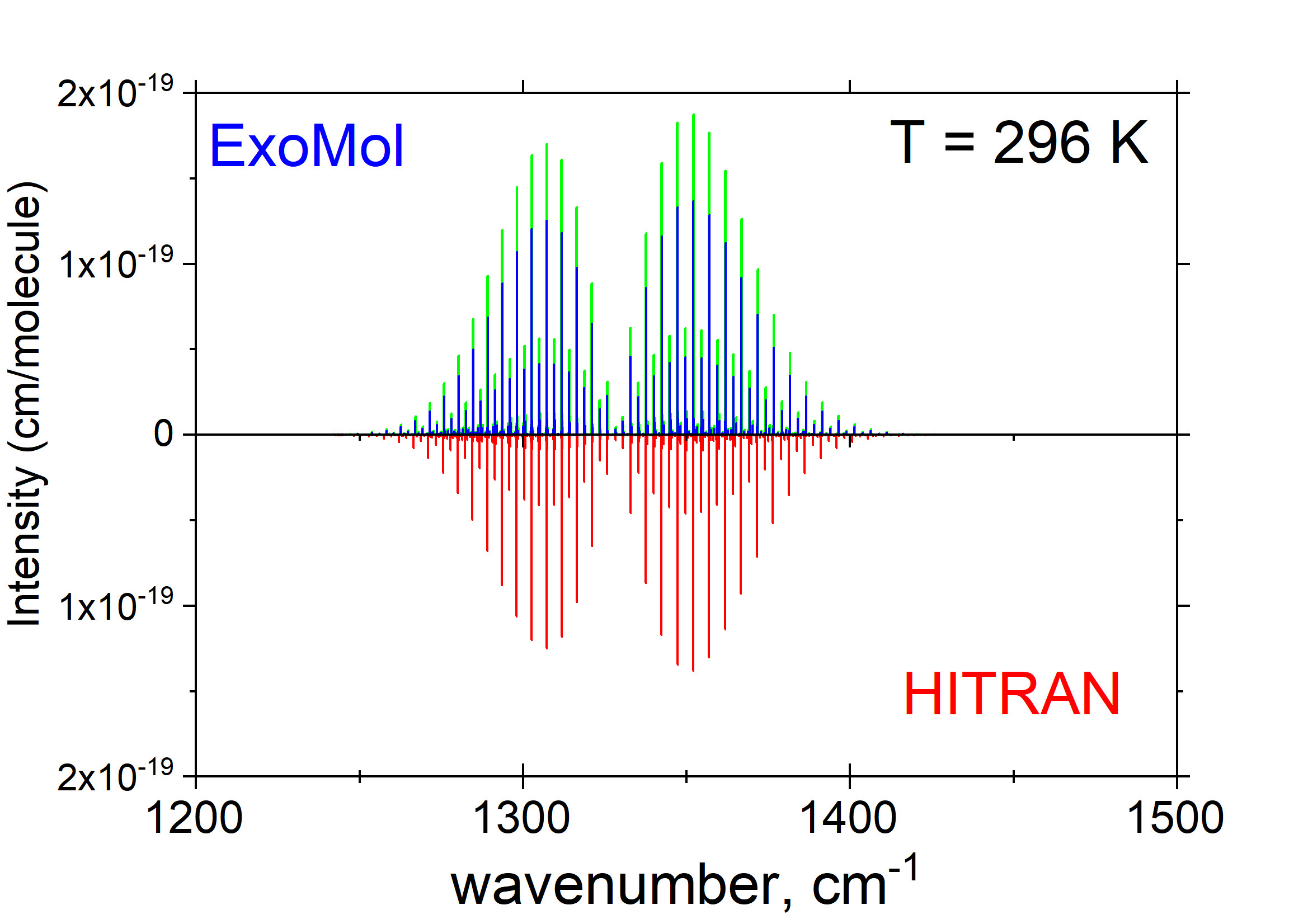
Figure 1: Comparison of aCeTY (this work) stick spectra, before (green) and after (blue) dipole moment scaling by a factor of 0.856, against HITRAN for the vibrational band (000110) $\Sigma_{u}^{+}$ of acetylene at $T=$ 296 K.

3 Results: the aCeTY line list

The aCeTY line list has been computed using the variational calculations outlined above. Figure 2 illustrates the temperature-dependence of the acetylene spectra computed using the aCeTY line list, with cross-sections computed using ExoCross (Yurchenko et al., 2018) at a variety of temperatures between 296–2000 K. The cross-sections are calculated at a low-resolution of 1 cm^-1 for demonstration purposes.

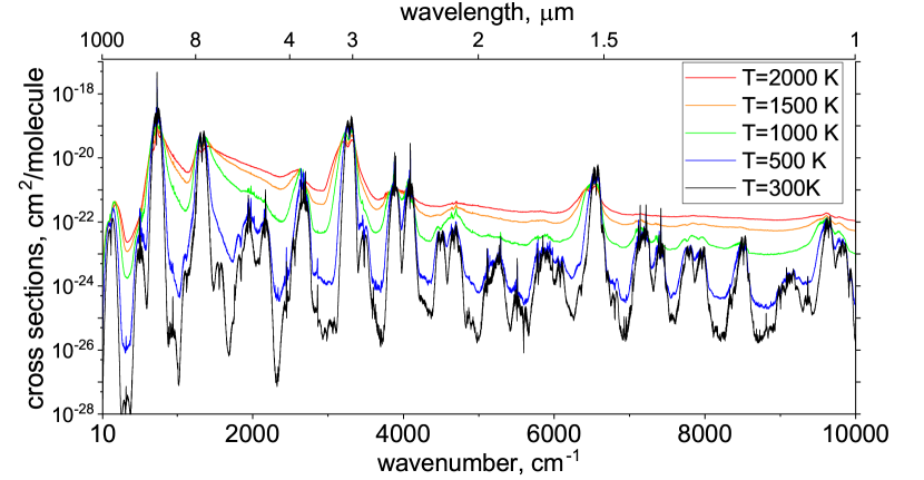
Figure 2: Variation of aCeTY line list spectra with temperature: low-resolution (1 cm^-1) cross-sections computed using ExoCross (Yurchenko et al., 2018). The spectrum becomes flatter with increasing temperature.

The TROVE assignment is based on the largest basis set contribution to the eigenfunction. TROVE uses the local mode quantum numbers (QNs) to assign vibrational state, collected in Table 1. This selection of the quantum numbers is based on the choice of the vibrational basis set in Eqs. (3–5). There is no direct correlation between the local mode and normal mode assignment. For an approximation correlation, the following rules apply:

$$\upsilon_{1}+\upsilon_{3} = n_{2}+n_{3},$$ (16)

$$\upsilon_{2} = n_{1},$$ (17)

$$\upsilon_{4}+\upsilon_{5} = n_{4}+n_{5}+n_{6}+n_{7}.$$ (18)

The number density of a particular molecular state as a fraction of the total number density of the molecular species is given by the Boltzmann law. The total internal partition function, $Q$, is a sum over all molecular states, weighting each by their probability of occupation at a given temperature, and therefore offers an indication of the completeness of a calculated line list at a particular temperature:

$$Q=\sum_{i=1}^{N}{g_{ns}}^{(i)}(2J_{i}+1)\exp\left({\frac{-c_{2}\tilde{E}_{i}}{T}}\right).$$ (19)

Here, c₂=$\frac{hc}{k}$ is the second radiative constant, $\tilde{E}_{i}$ is the energy term value of each $i$ molecular state (relative to the ground ro-vibronic state), $T$ is the temperature, ${g_{ns}}^{(i)}$ is the nuclear statistical weight of each $i$ molecular state, and the sum is over all molecular states. The partition function can easily be computed from the ExoMol states file (Tennyson et al., 2016) using ExoCross (Yurchenko et al., 2018). A comparison of the partition function for ¹²C₂H₂ computed using the aCeTY states file against the partition function computed using TIPS (Gamache et al., 2017), the coefficients by Irwin (1981) and the energies extracted from the ASD-1000 database of Lyulin & Perevalov (2017) is given in Figure 3. All these partition functions, with the exception of the one due to (Irwin, 1981), use the “physicists” convention which weights ortho and para states of ¹²C₂H₂ 3 and 1, respectively, as opposed to the weighting of 0.75 and 0.25 often adopted by astronomers.

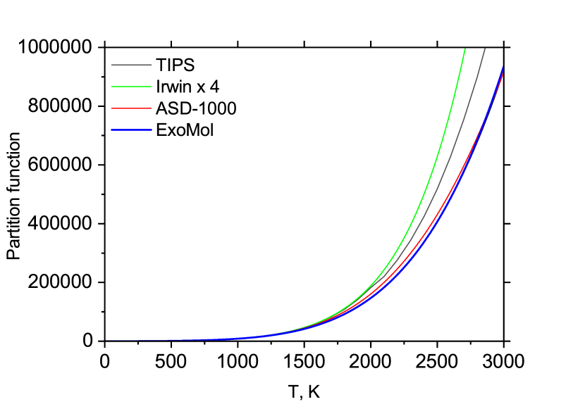
Figure 3: The ¹²C₂H₂ partition function up to 3000 K; comparing the states from the aCeTY line list (this work) against that computed using TIPS (Gamache et al., 2017), the coefficients of Irwin (1981), and using energies extracted from ASD-1000 (Lyulin & Perevalov, 2017).

The temperature at which a line list is complete up to is generally dictated by the range of energy levels included in a line list production. For the aCeTY line list we use a maximum lower energy of 12 000 cm^-1, and a maximum upper energy of 22 000 cm^-1, which gives a line list that is complete up to 10 000 cm^-1 (i.e. $\lambda>1$ $\mu$m), i.e. the maximum upper energy is 10 000 cm^-1 above the maximum lower energy level value. The completeness as a function of temperature of such a line list can be estimated by calculating the partition function up to the lower energy level cut-off as a percentage of the total partition function which includes all states involved in a line list calculation. Figure 5 gives these values at a variety of temperatures. A line list is generally considered to be “complete” if the ratio of the partition function of the lower energy states to the partition function of all energy states involved in a line list calculation is $>90\%$. It can be seen from Figure 5 that the aCeTY line list is therefore estimated, using this metric, to be complete up to around 2200 K. The other factor which could have an impact on the completeness of the line list is the value used for $K_{\rm max}=L_{\rm max}$ in Eq. (2). As discussed, however, we do not expect the states below 22 000 cm^-1 which are being used for the line list to have high values of $L_{\rm max}$; the bending states which correspond to a high value of $L$ are expected at very high energies, and therefore temperatures. Figure 4 shows the contributions from transitions with upper states with different values of $K$ ($=L$) to a line list computed up to $K_{\rm max}=L_{\rm max}$ = 16. It can be seen that states with higher values of $K$ contribute a vanishingly small amount to the overall opacity. We therefore do not expect increasing the value of $K_{\rm max}=L_{\rm max}$ in a calculation to have a significant effect on the opacity of a acetylene even at high temperatures.

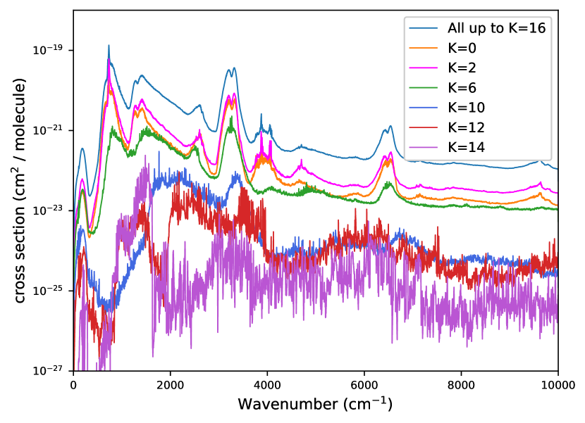
Figure 4: Contribution from transitions with upper states of different $K^{\prime}$ to the aCeTY opacity at $T$ = 2000 K. Note that the $K^{\prime}$ = 16 transitions do not appear on this scale.

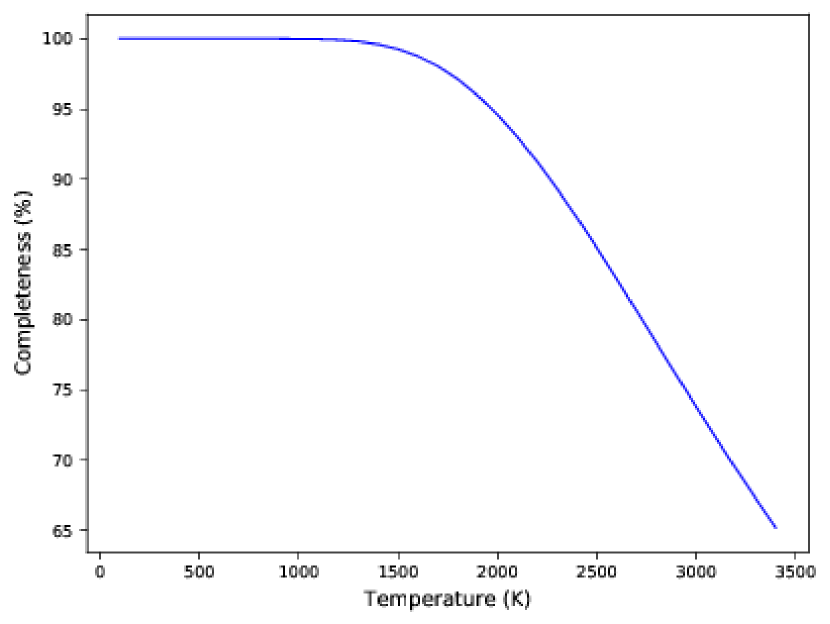
Figure 5: The completeness of the aCeTY line list as a function of temperature, up to 3400 K.

A complete description of the ExoMol data structure along with examples was reported by Tennyson et al. (2016). The ExoMol .states file contains all computed ro-vibrational energies (in cm^-1) relative to the ground state. Each energy level is assigned a unique state ID with symmetry and quantum number labelling; an extract for ¹²C₂H₂ is shown in Table 3. The .trans files, which are split into frequency windows for ease of use, contain all computed transitions with upper and lower state ID labels, and Einstein A coefficients. An example from a .trans file for the aCeTY line list is given in Table 4.

Table 3: Extract from the .states file for the aCeTY line list. The theoretical energies were replaced with MARVEL where available (see text).

$N$	$\tilde{E}$	$g_{\text{tot}}$	$J$	Unc.	$\Gamma_{\text{tot}}$	$n_{1}$	$n_{2}$	$n_{3}$	$n_{4}$	$n_{5}$	$n_{6}$	$n_{7}$	$\Gamma_{\text{vib}}$	$K$	$\tau_{\text{rot}}$	$\Gamma_{\text{rot}}$	$\tilde{E}^{\rm TROVE}$
793042	14.119512	21	3	0.000041	A2g	0	0	0	0	0	0	0	A1g	0	1	A2g	14.117789
793043	625.7974	21	3	0.000204	A2g	0	0	0	0	0	0	1	E1g	1	1	E1g	625.793876
793044	1242.947091	21	3	0.000434	A2g	0	0	0	0	1	0	1	E2g	2	0	E2g	1242.933977
793045	1244.544497	21	3	0.000368	A2g	0	0	0	1	0	1	0	A1g	0	1	A2g	1244.546193
793046	1463.286132	21	3	0.000266	A2g	0	0	0	0	0	0	2	A1g	0	1	A2g	1463.285595
793047	1472.462847	21	3	0.000532	A2g	0	0	0	0	1	0	1	E2g	2	0	E2g	1472.455065
793048	1865.740794	21	3	1	A2g	0	0	0	1	0	1	1	E3g	3	1	E3g	-1
793049	1868.702371	21	3	0.001250	A2g	0	0	0	0	2	0	1	E1g	1	1	E1g	1868.70286
793050	1988.361458	21	3	0.001649	A2g	1	0	0	0	0	0	0	A1g	0	1	A2g	1988.353787
793051	2062.011051	21	3	0.001087	A2g	0	0	0	0	3	0	0	E1g	1	1	E1g	2062.010327
793052	2080.003537	21	3	0.001923	A2g	0	0	0	2	0	0	1	E1g	1	1	E1g	2080.003632
793053	2088.260006	21	3	1	A2g	0	0	0	2	1	0	0	E3g	3	1	E3g	-1
793054	2500.471967	21	3	2	A2g	0	0	0	0	2	0	2	E2g	2	0	E2g	-1
793055	2502.756348	21	3	2	A2g	0	0	0	2	0	2	0	A1g	0	1	A2g	-1
793056	2587.563753	21	3	0.001414	A2g	1	0	0	0	0	0	1	E1g	1	1	E1g	2587.571805
793057	2662.227679	21	3	0.004000	A2g	0	0	0	0	2	0	2	A1g	0	1	A2g	2662.229753
793058	2675.549505	21	3	2	A2g	0	0	0	2	0	2	0	E2g	2	0	E2g	-1
793059	2699.065141	21	3	2	A2g	0	0	0	2	0	0	2	A1g	0	1	A2g	-1
793060	2703.164786	21	3	2	A2g	0	0	0	2	1	0	1	E2g	2	0	E2g	-1
793061	2894.449628	21	3	0.000970	A2g	0	0	0	4	0	0	0	A1g	0	1	A2g	2894.449274

$N$ : State ID;

$\tilde{E}$: Term value (in cm^-1);

$g_{\text{tot}}$: Total degeneracy;

$J$: Total angular momentum;

$\Gamma_{\text{tot}}$: Total symmetry in ${\mathcal{D}}_{\infty{\rm h}}$(M)

$n_{1}$-$n_{7}$: TROVE vibrational quantum numbers (QN) (see Eq. (16));

$\Gamma_{\text{vib}}$: Symmetry of vibrational component of state in D_∞h(M);

$K$: Projection of $J$ on molecule-fixed $z$-axis ($K=L$);

$\tau_{\text{rot}}$: Rotational parity (0 or 1);

$\Gamma_{\text{rot}}$: Symmetry of rotational component of state in D_∞h(M);

$\tilde{E}^{\rm TROVE}$: TROVE term value, if replaced with MARVEL (in cm^-1);

Unc.: Uncertainty (cm^-1).

Table 4: Extract from a .trans file for the aCeTY line list.

$f$	$i$	$A_{fi}$
56645	1	2.19617648E-05
56554	1	4.23999064E-02
56923	1	3.00213998E-03
56736	1	8.28753699E-09
56839	1	8.60646693E-07
56646	1	1.25543720E-05
56555	1	8.33151532E-04
56924	1	2.58105436E-06

$f$: Upper state ID;
$i$: Lower state ID;
$A_{fi}$: Einstein A coefficient (in s^-1).

4 Comparison to Other Data

Figure 6 shows an overview of an absorption spectrum of ¹²C₂H₂ computed using aCeTY (this work) to that produced using HITRAN-2016 (Gordon et al., 2017) at $T=$ 296 K for the wavenumber range from 0 to 10 000 cm^-1. Apart from some missing weak bands in HITRAN, it shows a generally good agreement. Figures 7 and 8 give more detailed comparisons of the main bands of ¹²C₂H₂ in the range 0–10 000 cm^-1 with the data from HITRAN-2016 (Gordon et al., 2017), again in the form of stick spectra (absorption coefficients) at room-temperature. The overall agreement of the line positions and intensities is good, except several weaker bands of C₂H₂, overestimated by aCeTY, as well as bands not present in HITRAN. Table 2 gives a summary of the accuracy of the line positions for $J\leq 5$ states presented in Marvel and used in the refinement and band-centre corrections. The full table is given as supplementary information to this work.

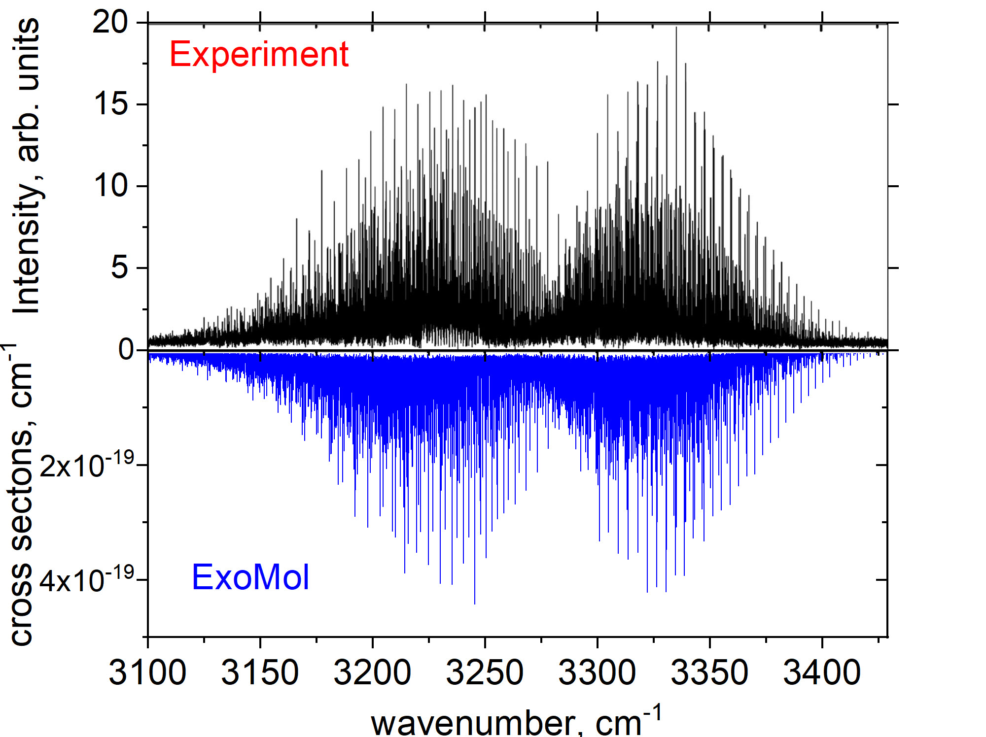
Figure 9: Comparison of the acetylene spectra in the 3$\mu$m region computed using aCeTY at $T=1355$ K with the experimental data by Amyay et al. (2009). The aCeTY cross-sections were generated using ExoCross and a Voigt line profile assuming $P=1$ atm.

Figure 9 shows the hot spectrum (cross-sections) of the 3 $\mu$m band of C₂H₂ at $T=1355$ K compared to the experimental data by Amyay et al. (2009) demonstrating the generally good agreement also at high temperatures.

The ASD-1000 database of Lyulin & Perevalov (2017) is a calculated acetylene line list which covers transitions up 10 000 cm^-1 and $J$=100, based on the use of an effective Hamiltonian fit to experimental data and extrapolated to higher energies. The energies and intensities at room-temperature agree reasonably well with those in the HITRAN-2016 (Gordon et al., 2017) database (see Lyulin & Perevalov (2017) and Lyulin & Campargue (2017) for detailed comparisons), and ASD-1000 has been used to update the 2016 HITRAN release in the low energy region (Gordon et al., 2017; Jacquemart et al., 2017). Figure 10 gives a comparison of cross-sections computed using the aCeTY and ASD-1000 line lists at $T=1000$ K. The results are significantly different and it would appear that ASD-1000 fails to adequately account for the many hot bands which become important at higher temperatures.

A comparison with PNNL is given in Figure 11, for $T=50^{\circ}$.

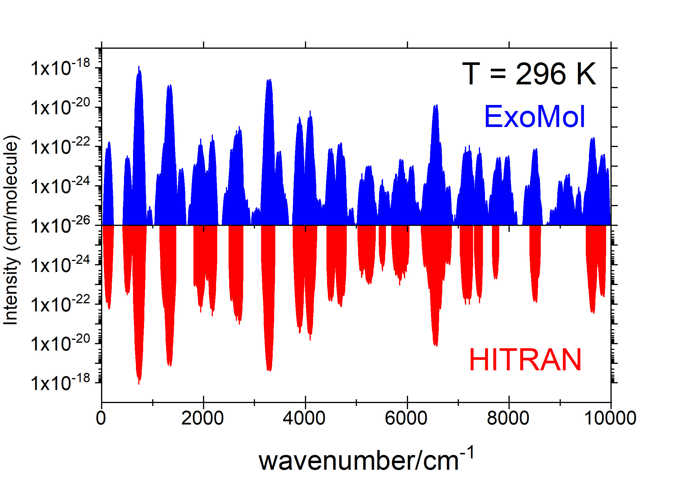
Figure 6: Comparison of the aCeTY stick spectrum with the HITRAN data for the range up to 10 000 cm^-1 at 296 K.

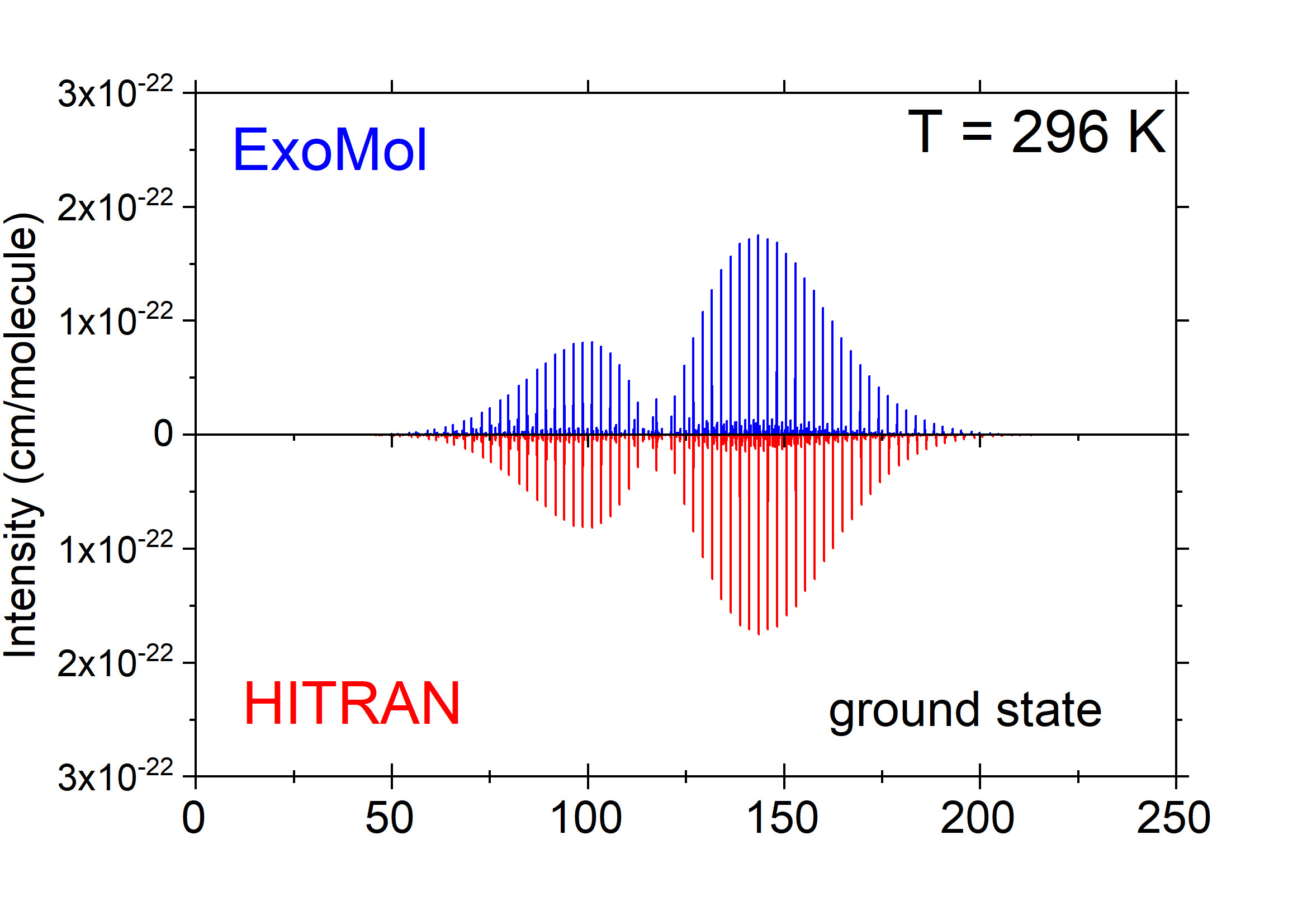
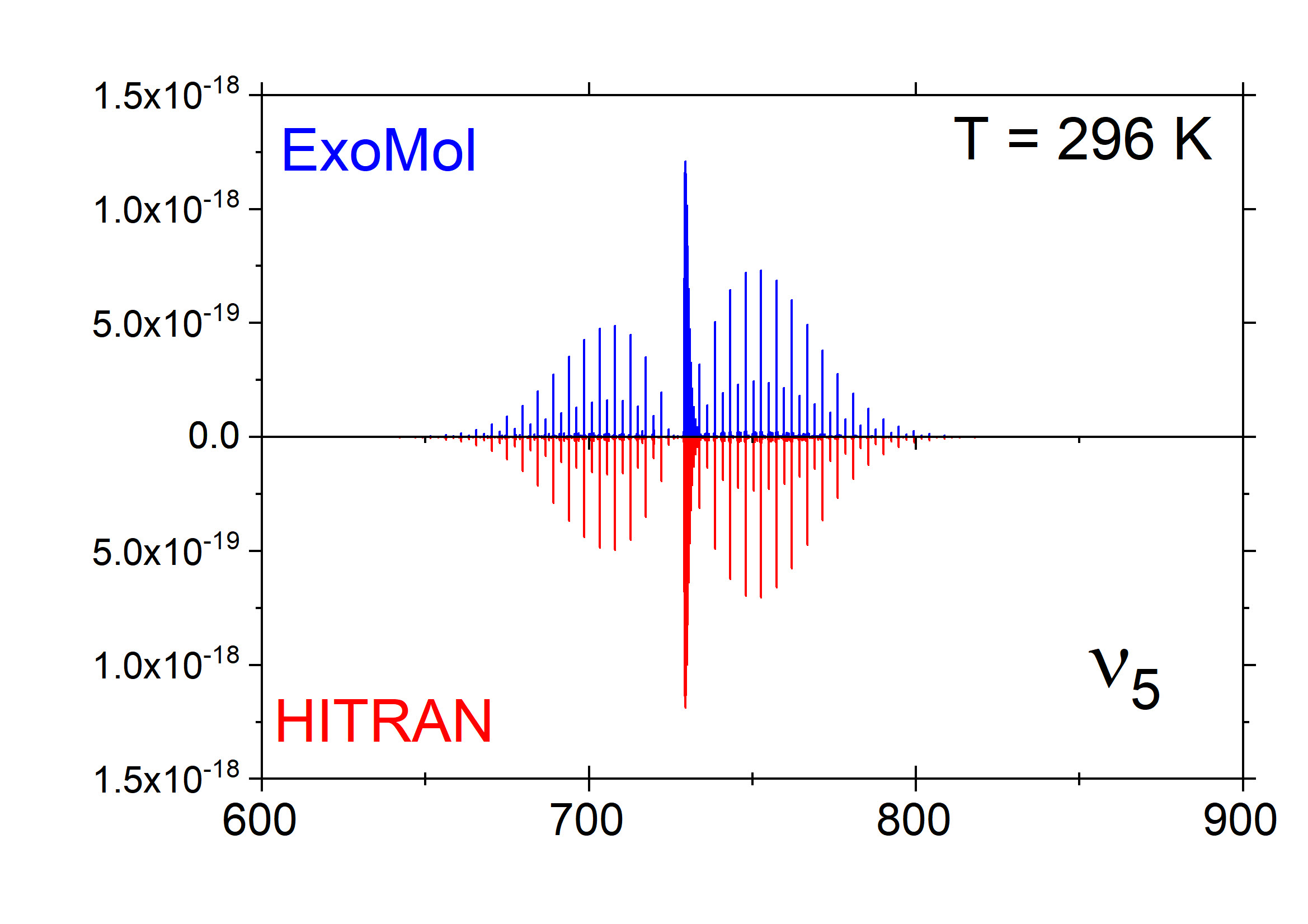
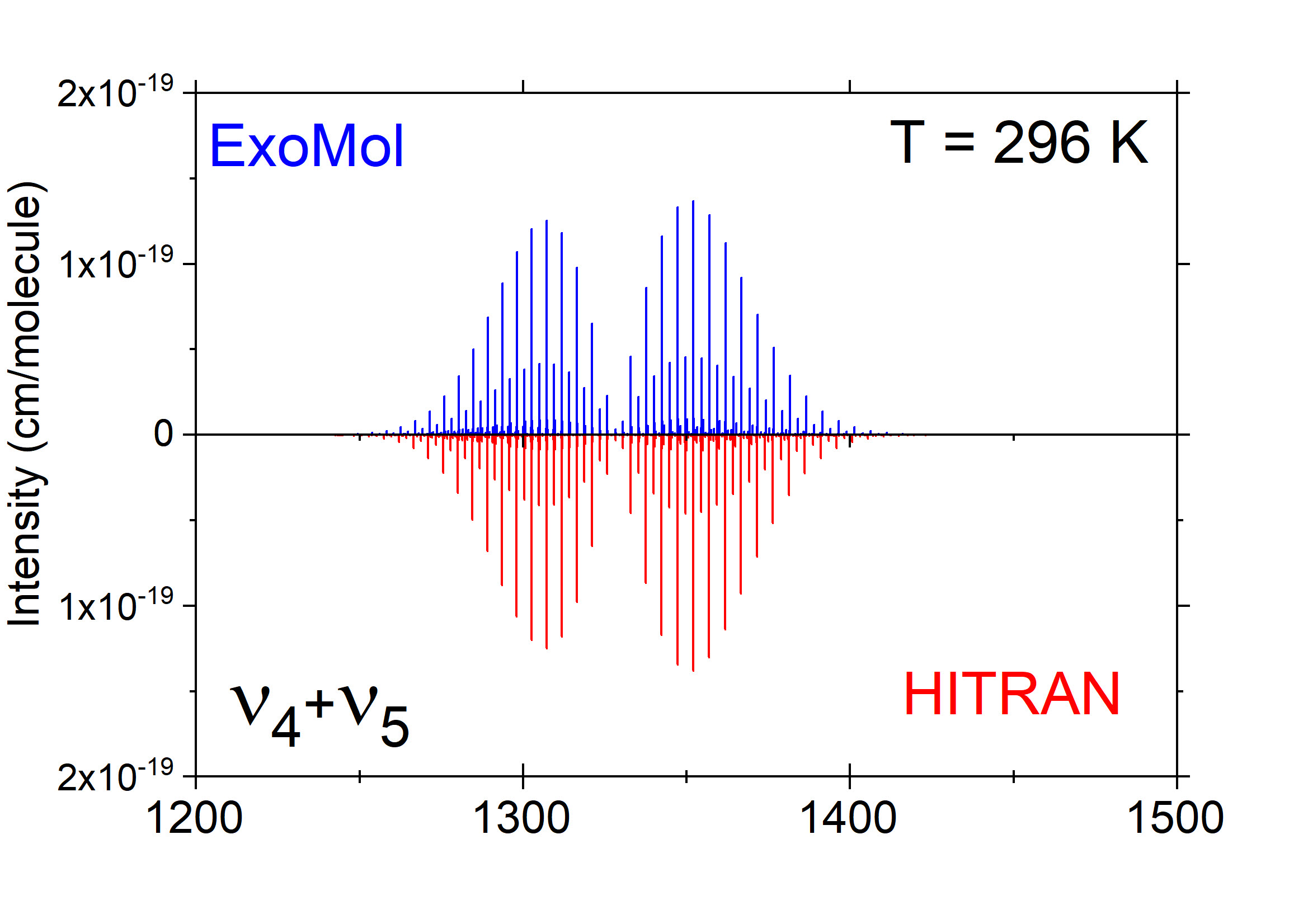
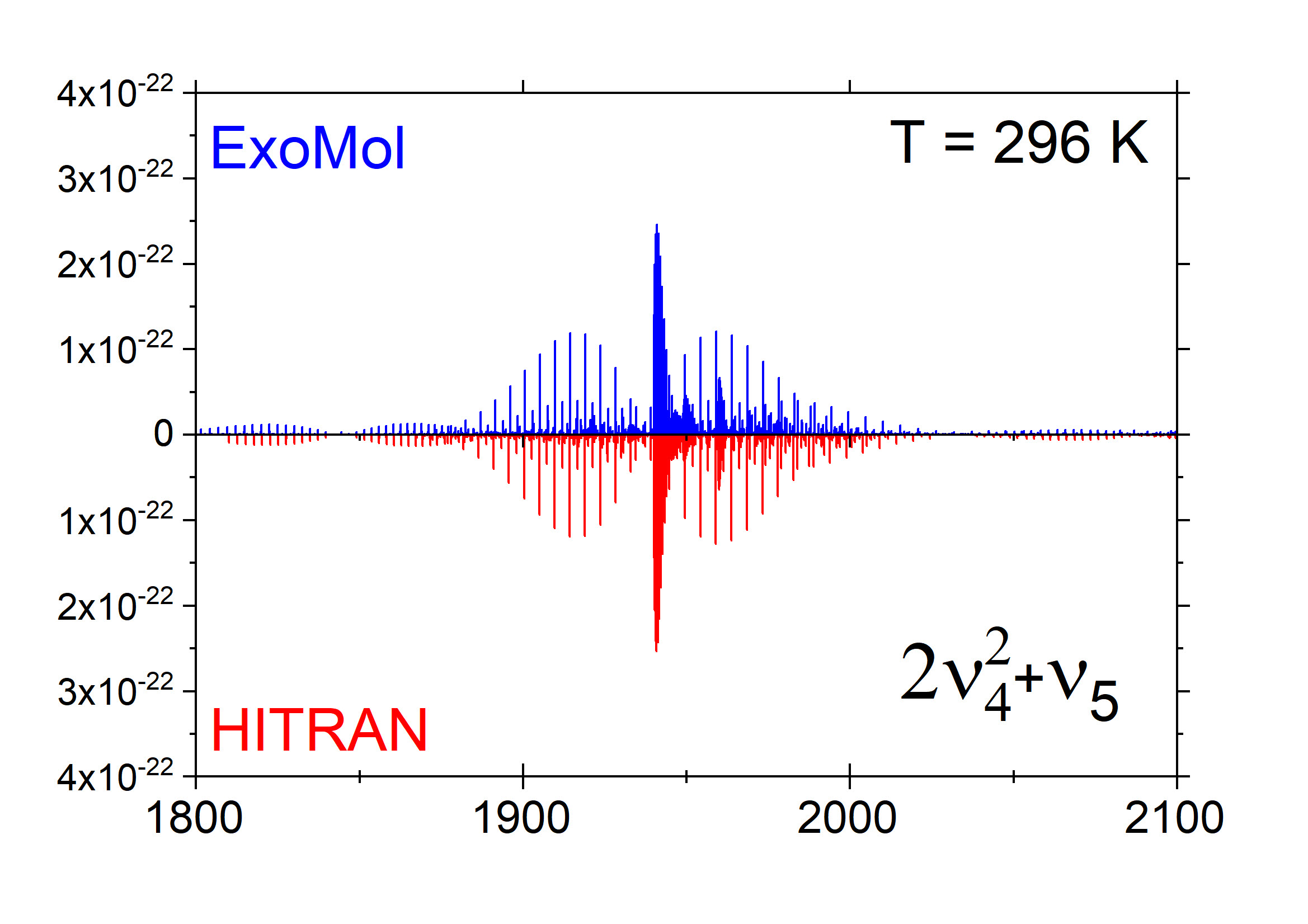
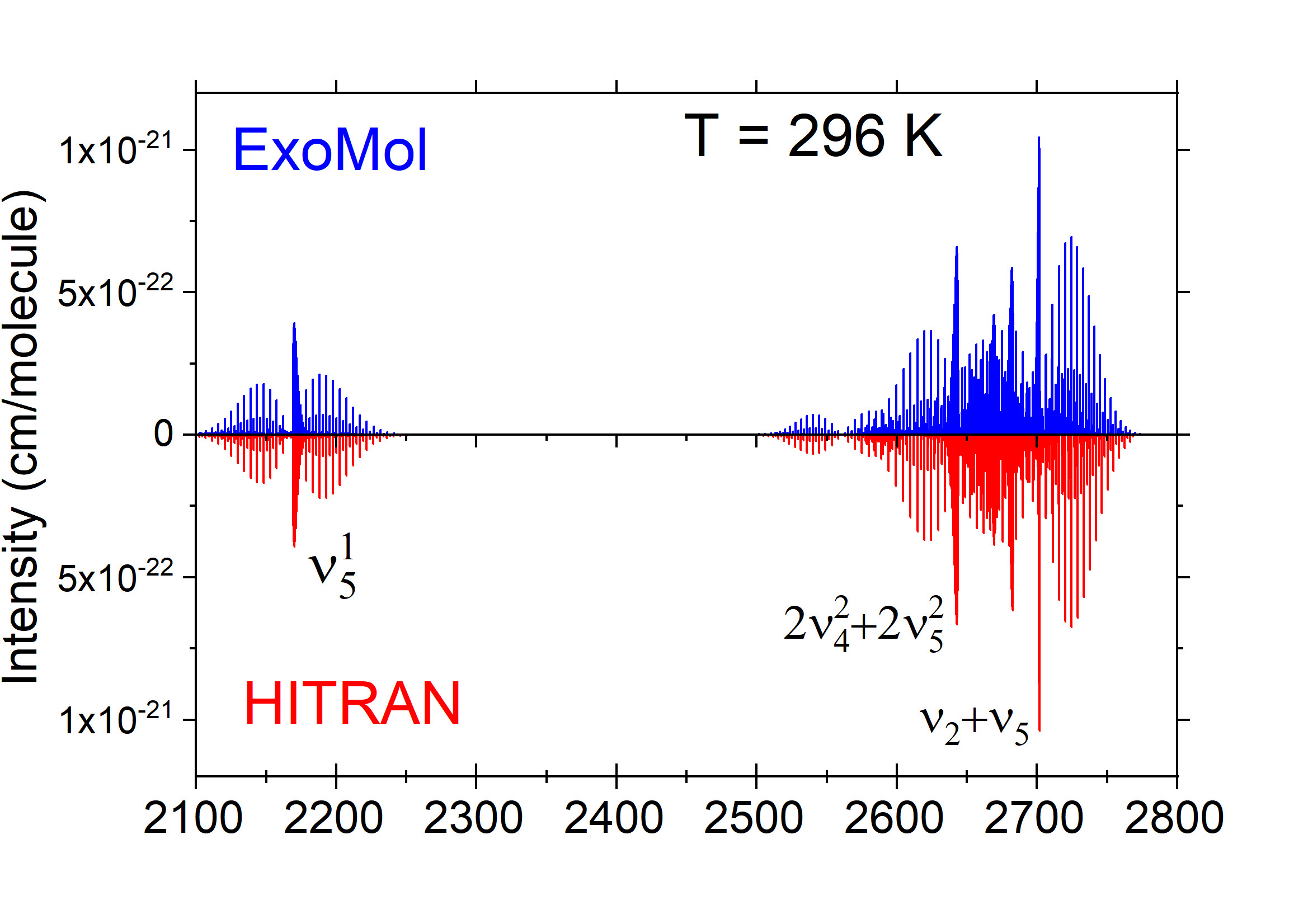
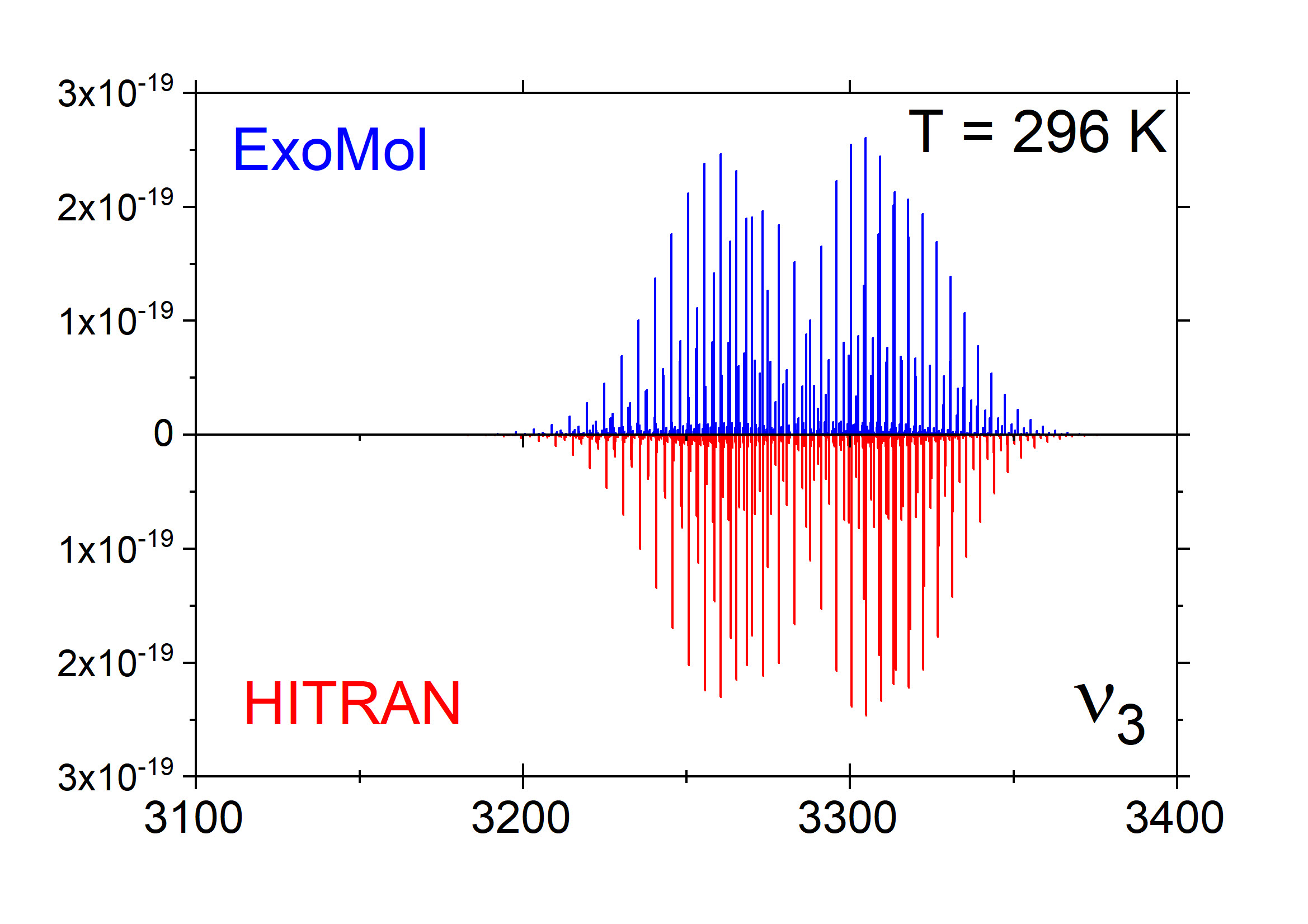
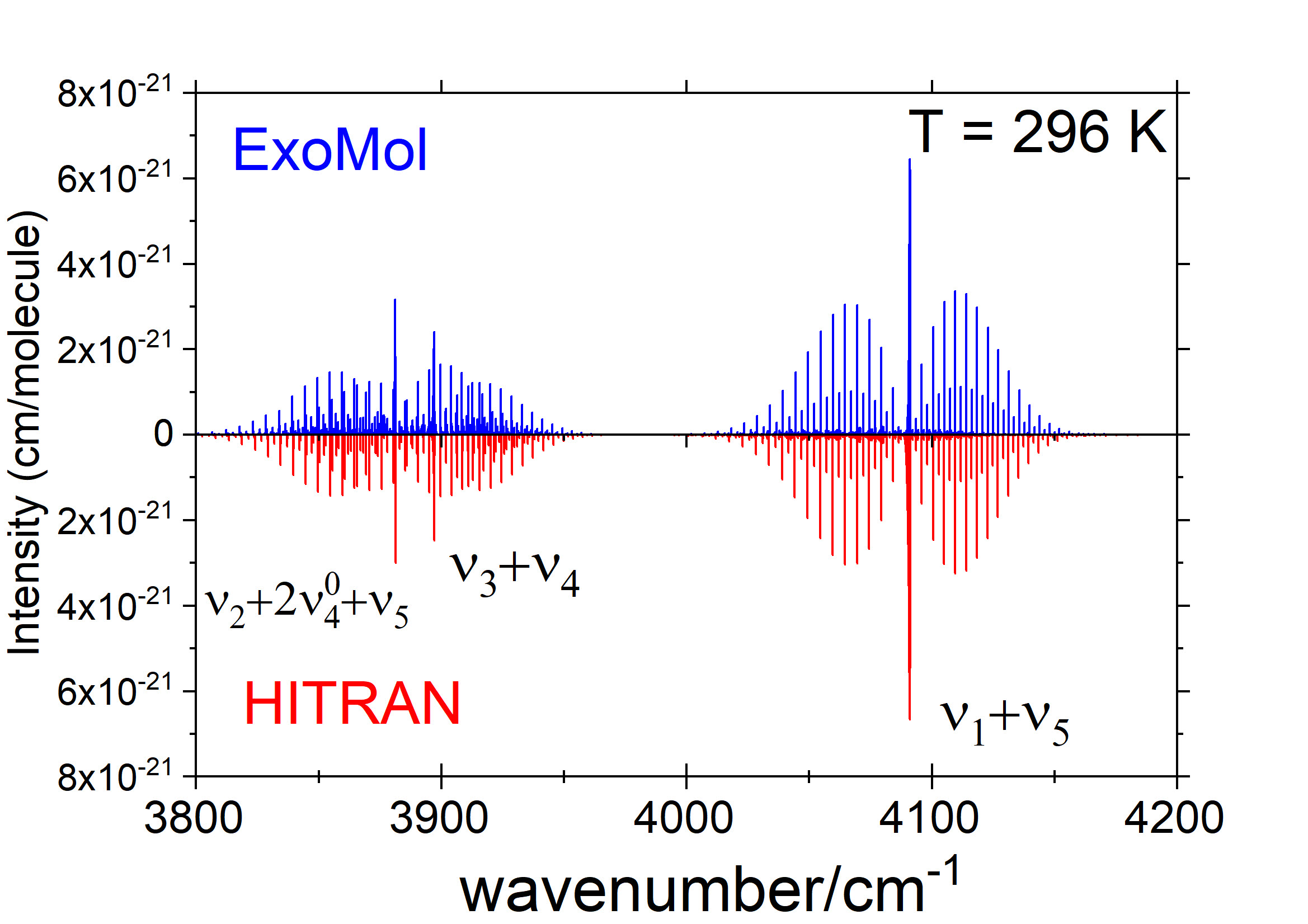
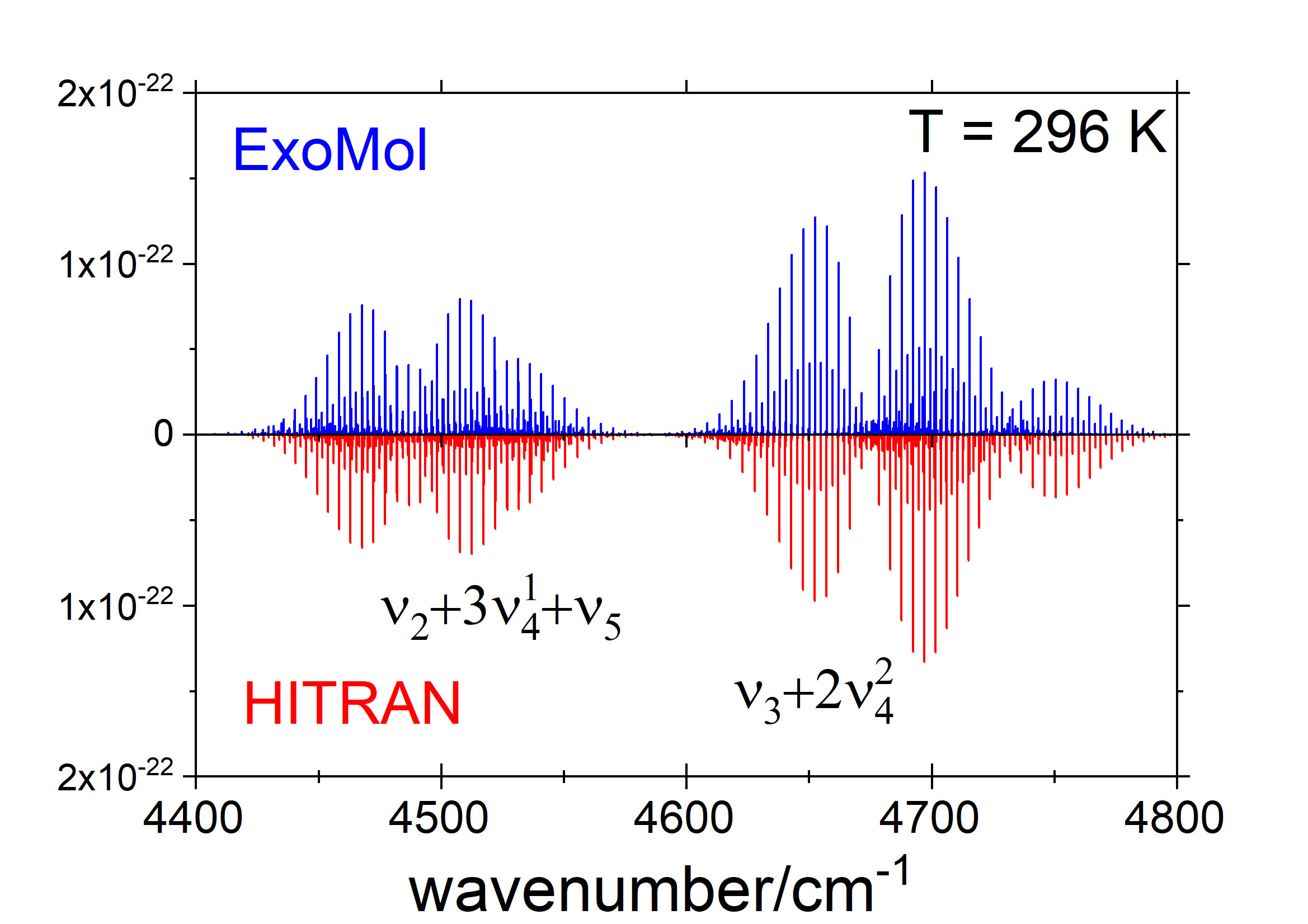
Figure 7: Comparison of the aCeTY stick spectra (with scaling of the dipole moment applied) against HITRAN for different vibrational bands of acetylene at 296 K (in the range 0-5000 cm^-1). The vibrational assignment of the strongest bands is shown.

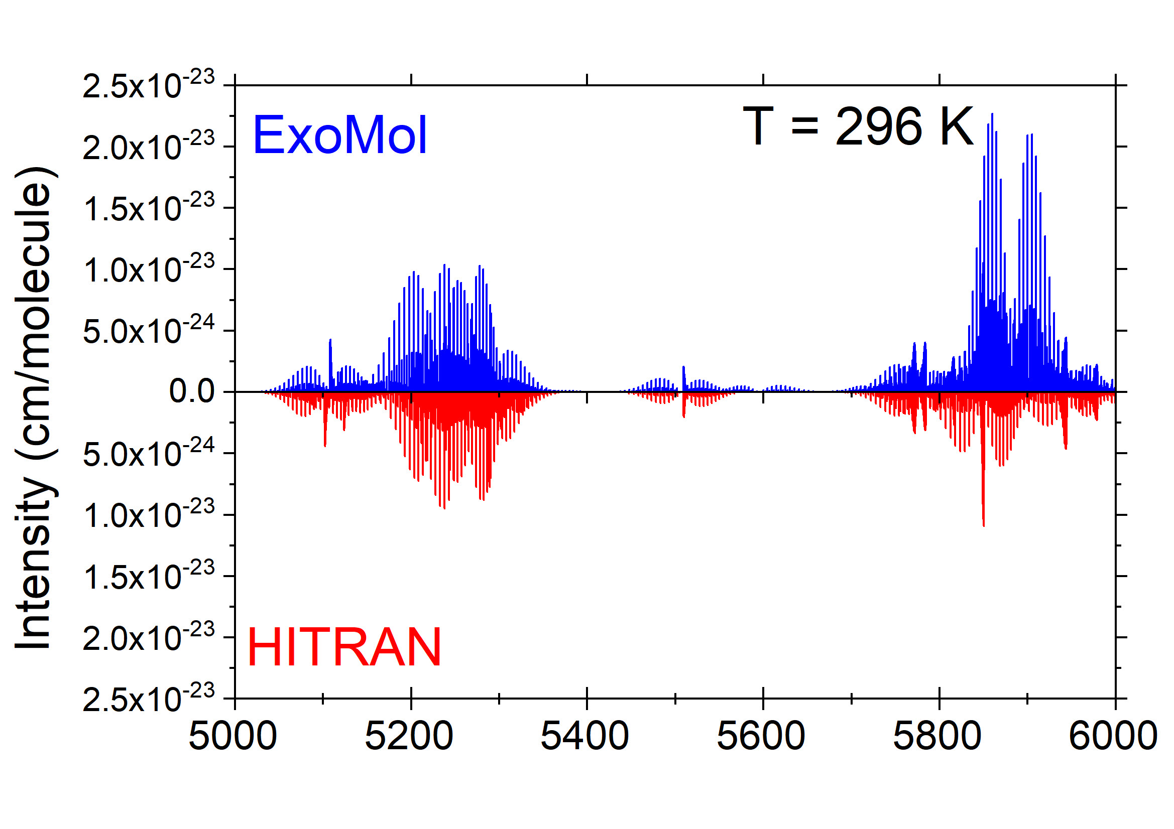
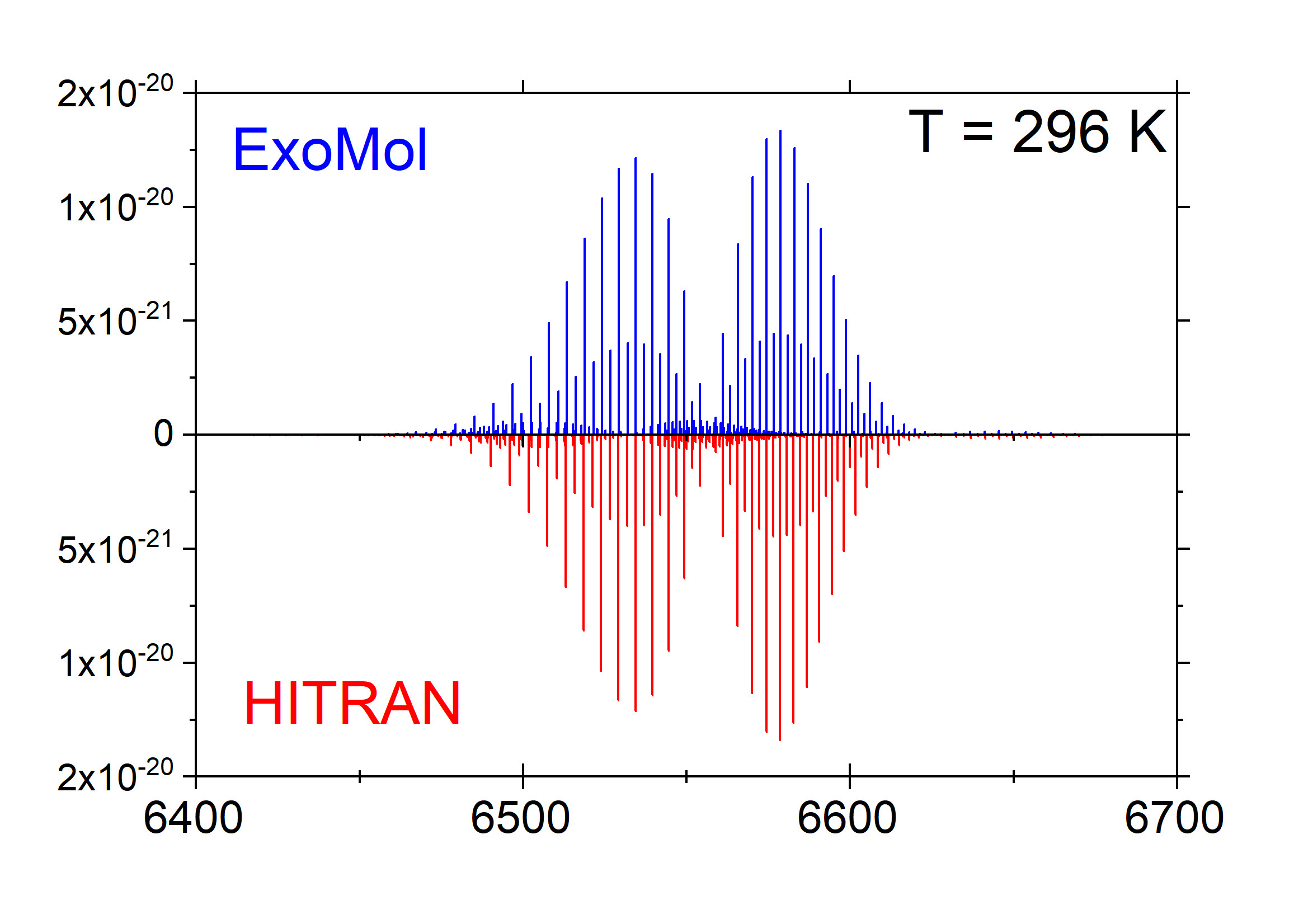
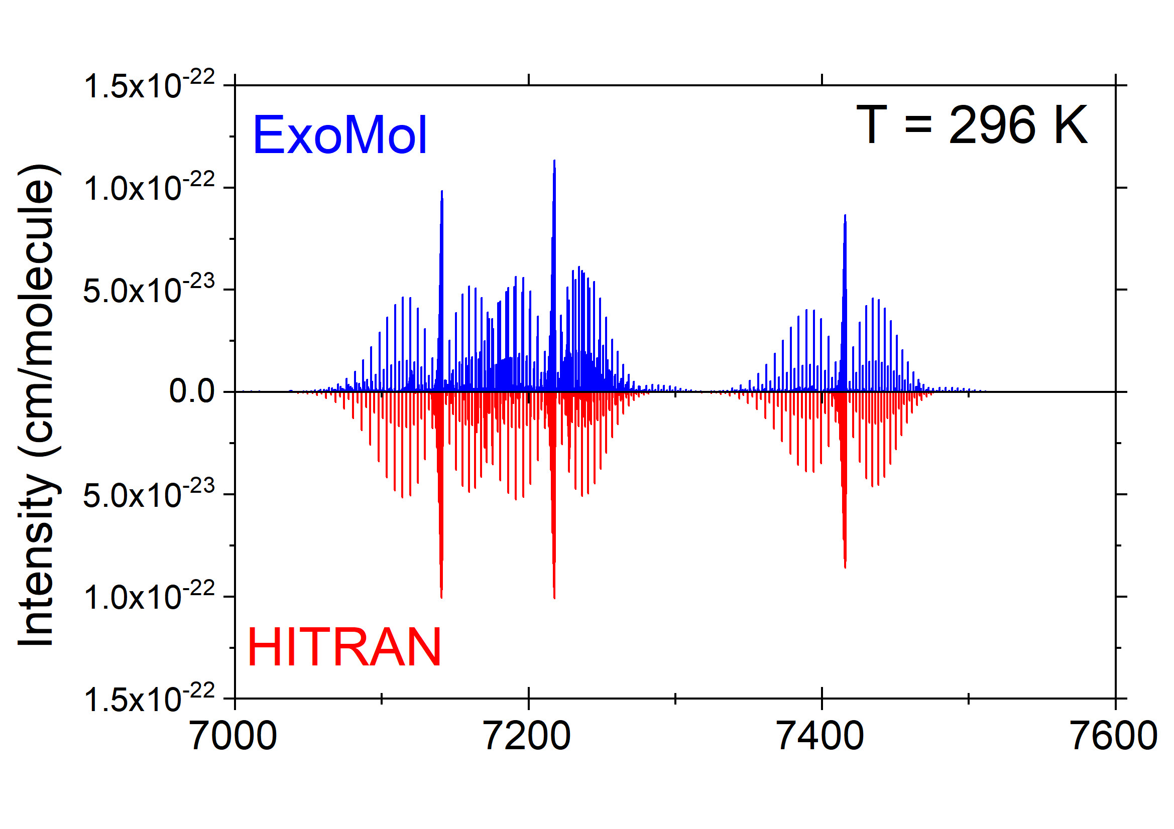
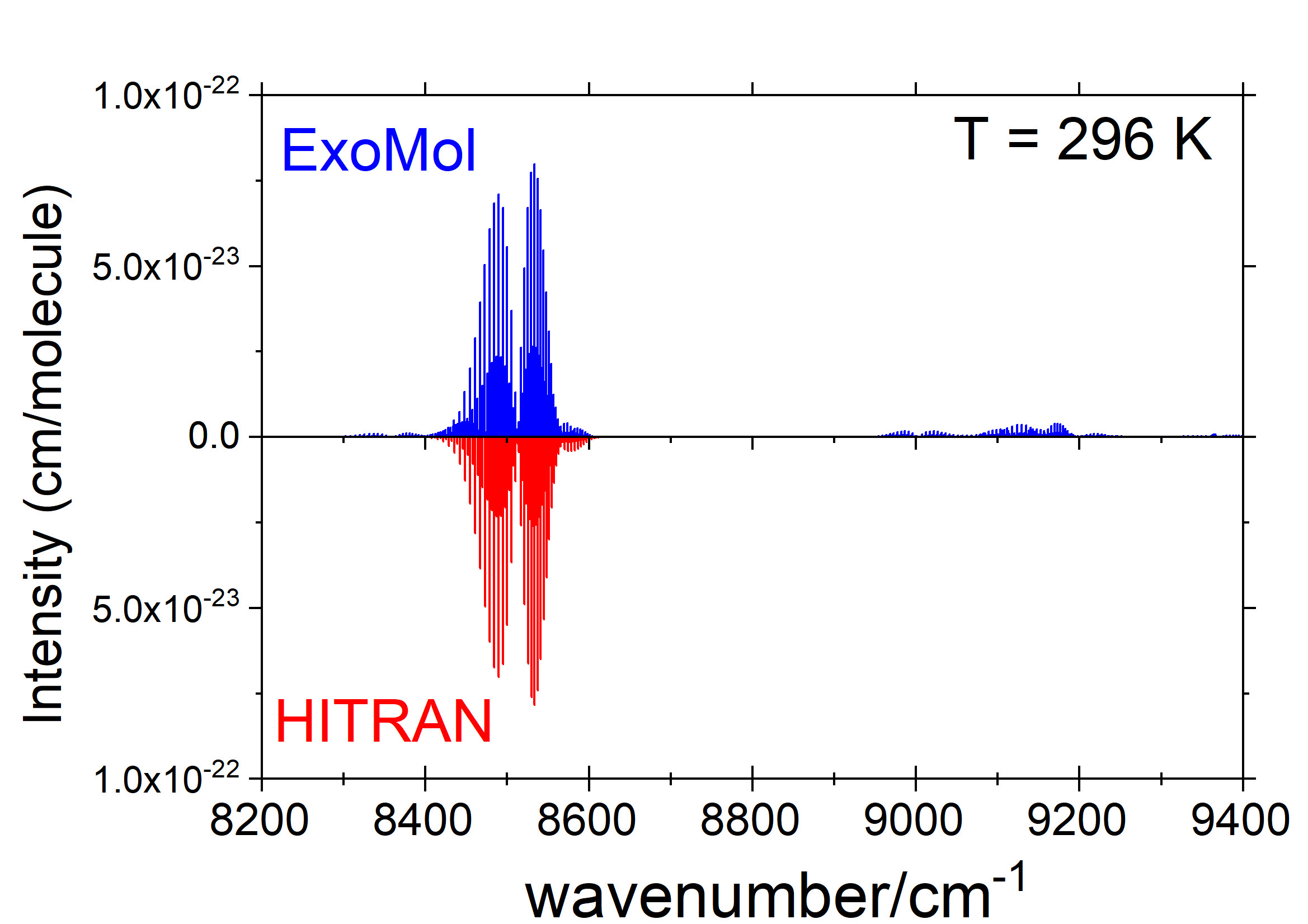
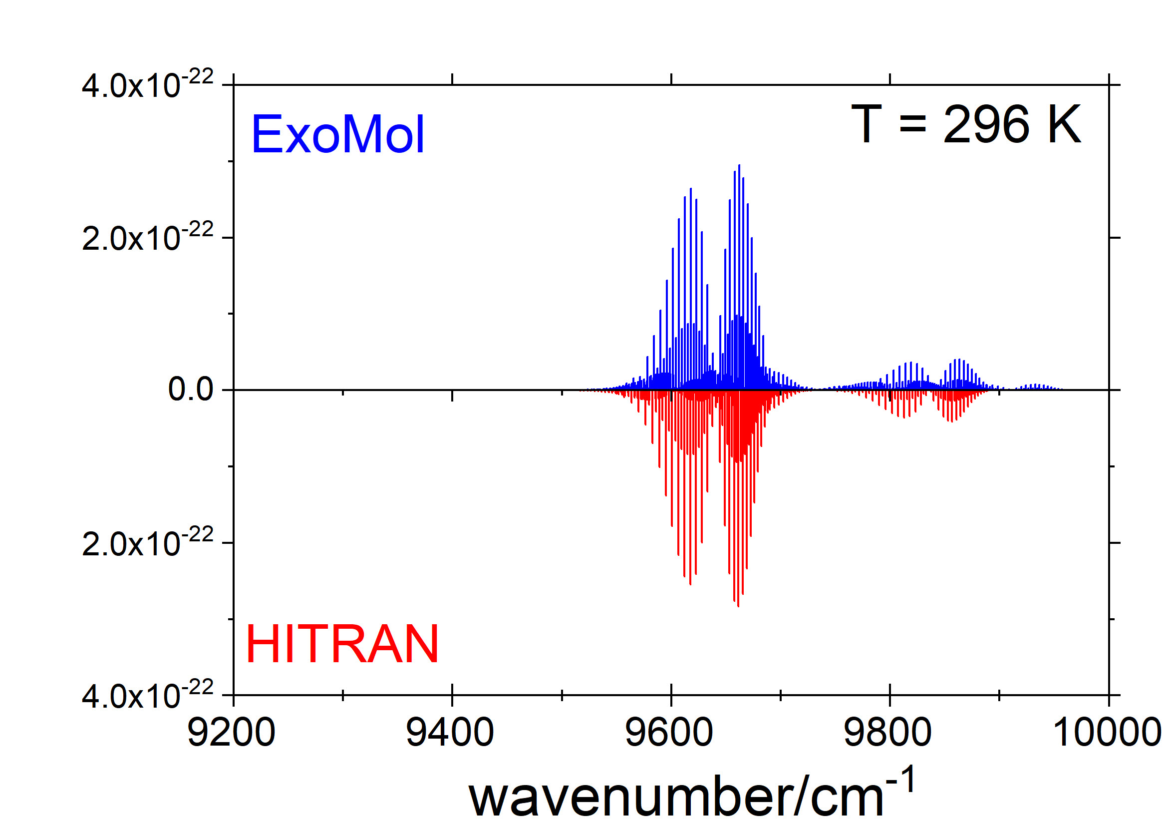
Figure 8: Comparison of the aCeTY stick spectra against HITRAN (with scaling of the dipole moment applied) against HITRAN for different vibrational bands of acetylene at 296 K (in the range 5000-10 000 cm^-1).

Table 5: An extract of vibrational transition dipole moment scaling factors, $f_{\mu}=\sqrt{\bar{S}}$, used to produce the line list for fundamental and overtone bands. $\sqrt{\bar{S}}$ is the band intensity scaling factor. The full table is given as part of the supplementary information to this work.

$\Gamma$	$\upsilon_{1}$	$\upsilon_{2}$	$\upsilon_{3}$	$\upsilon_{4}$	$l_{4}$	$\upsilon_{5}$	$l_{5}$	$L$	$E_{i}/hc$	$f_{\mu}$
$\Pi_{u}$	0	0	0	0	0	1	1	1	730.33	1.0181
$\Sigma_{u}^{+}$	0	0	0	1	1	1	-1	0	1328.07	0.8561
$\Delta_{u}$	0	0	0	1	1	1	1	2	1347.51	0.9813
$\Pi_{u}$	0	0	0	2	2	1	-1	1	1941.18	0.3653
$\Pi_{u}$	0	0	0	2	0	1	1	1	1960.87	1.3899
$\Pi_{u}$	0	0	0	0	0	3	1	1	2170.34	1.0429
$\Sigma_{u}^{+}$	0	0	0	3	1	1	-1	0	2560.59	1.7062
$\Pi_{u}$	0	1	0	0	0	1	1	1	2703.10	1.0271
$\Sigma_{u}^{+}$	0	1	0	1	1	1	-1	0	3281.91	1.0268
$\Sigma_{u}^{+}$	0	0	1	0	0	0	0	0	3294.85	0.8923
$\Pi_{u}$	0	1	0	2	0	1	1	1	3882.42	0.8122
$\Pi_{u}$	0	0	1	1	1	0	0	1	3898.34	0.5774
$\Pi_{u}$	1	0	0	0	0	1	1	1	4092.34	0.9985
$\Pi_{u}$	0	1	0	0	0	3	1	1	4140.08	0.9636
$\Sigma_{u}^{+}$	0	1	0	3	1	1	-1	0	4488.85	0.6464
$\Sigma_{u}^{+}$	0	0	1	2	0	0	0	0	4508.02	0.7419
$\Sigma_{u}^{+}$	1	0	0	1	1	1	-1	0	4673.71	1.5789
$\Sigma_{u}^{+}$	0	0	1	0	0	2	0	0	4727.07	0.8830

Table 6: An extract of the transition dipole moment scaling factors, $f_{\mu}=\sqrt{\bar{S}}$, used to produce the line list for hot bands starting from the $(000100)$ $\Pi_{g}$ state. $\sqrt{\bar{S}}$ is the band intensity scaling factor. The full table is given as part of the supplementary information to this work.

$\Gamma$	$\upsilon_{1}$	$\upsilon_{2}$	$\upsilon_{3}$	$\upsilon_{4}$	$l_{4}$	$\upsilon_{5}$	$l_{5}$	$L$	$E_{i}/hc$	$f_{\mu}$
$\Pi_{u}$	0	0	0	0	0	1	1	1	730.33	0.8730
$\Sigma_{u}^{+}$	0	0	0	1	1	1	-1	0	1328.07	1.0490
$\Delta_{u}$	0	0	0	1	1	1	1	2	1347.51	1.0312
$\Pi_{u}$	0	0	0	2	2	1	-1	1	1941.18	0.8233
$\Pi_{u}$	0	0	0	2	0	1	1	1	1960.87	1.5482
$\Sigma_{u}^{+}$	0	0	0	3	1	1	-1	0	2560.59	0.5440
$\Delta_{u}$	0	0	0	3	3	1	-1	2	2561.67	0.4387
$\Sigma_{u}^{-}$	0	0	0	3	1	1	-1	0	2583.84	1.3237
$\Pi_{u}$	0	1	0	0	0	1	1	1	2703.10	0.7272
$\Sigma_{u}^{+}$	0	0	0	1	1	3	-1	0	2757.80	1.2130
$\Delta_{u}$	0	0	0	1	1	3	1	2	2773.41	1.0312
$\Sigma_{u}^{-}$	0	0	0	1	1	3	-1	0	2783.63	0.9999
$\Delta_{u}$	0	0	0	1	-1	3	3	2	2796.30	1.1276
$\Sigma_{u}^{+}$	0	1	0	1	1	1	-1	0	3281.91	0.8752
$\Sigma_{u}^{+}$	0	0	1	0	0	0	0	0	3294.85	0.8065
$\Pi_{u}$	0	1	0	2	0	1	1	1	3882.42	1.1363
$\Pi_{u}$	0	0	1	1	1	0	0	1	3898.34	0.8653
$\Sigma_{u}^{+}$	1	0	0	1	1	1	-1	0	4673.71	0.9740
$\Sigma_{u}^{-}$	1	0	0	1	1	1	-1	0	4688.83	1.0084
$\Delta_{u}$	1	0	0	1	1	1	1	2	4692.06	0.9710

Table 7: Vibrational transition dipole moment scaling factors, $f_{\mu}=\sqrt{\bar{S}}$, used to produce the line list: hot bands starting from the $(0000011)$ $\Pi_{u}$ state. $\sqrt{\bar{S}}$ is the band intensity scaling factor.

$\Gamma$	$\upsilon_{1}$	$\upsilon_{2}$	$\upsilon_{3}$	$\upsilon_{4}$	$l_{4}$	$\upsilon_{5}$	$l_{5}$	$L$	$E_{i}/hc$	$f_{\mu}$
$\Sigma_{g}^{+}$	0	0	0	2	0	0	0	0	1230.38	1.3200
$\Delta_{g}$	0	0	0	2	2	0	0	2	1233.49	0.6750
$\Sigma_{g}^{+}$	0	0	0	0	0	2	0	0	1449.11	1.0060
$\Delta_{g}$	0	0	0	0	0	2	2	2	1463.00	0.9773
$\Sigma_{g}^{+}$	0	1	0	0	0	0	0	0	1974.35	1.0368
$\Pi_{g}$	0	0	0	1	1	2	0	1	2049.06	0.8462
$\Pi_{g}$	0	0	0	1	-1	2	2	1	2066.97	0.7603
$\Pi_{g}$	0	1	0	1	1	0	0	1	2574.76	0.8972
$\Sigma_{g}^{+}$	0	0	0	2	2	2	-2	0	2648.01	0.3475
$\Sigma_{g}^{-}$	0	0	0	2	2	2	-2	0	2661.16	0.4196
$\Delta_{g}$	0	0	0	2	2	2	0	2	2666.06	0.5947
$\Sigma_{g}^{+}$	0	0	0	0	0	4	0	0	2880.22	1.0651
$\Delta_{g}$	0	0	0	0	0	4	2	2	2894.04	1.0543
$\Sigma_{g}^{+}$	1	0	0	0	0	0	0	0	3372.84	0.9953
$\Pi_{g}$	1	0	0	1	1	0	0	1	3970.05	1.5178
$\Pi_{g}$	0	1	0	1	1	2	0	1	4002.46	1.2100
$\Pi_{g}$	0	0	1	0	0	1	1	1	4016.73	0.8622
$\Sigma_{g}^{+}$	1	0	0	0	0	2	0	0	4800.13	0.9912
$\Delta_{g}$	1	0	0	0	0	2	2	2	4814.19	0.9952

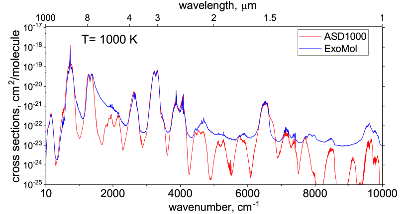
Figure 10: Comparison of the aCeTY line list with ASD-1000 (Lyulin & Perevalov, 2017); spectra computed up to 10 000 cm^-1 at 1000 K.

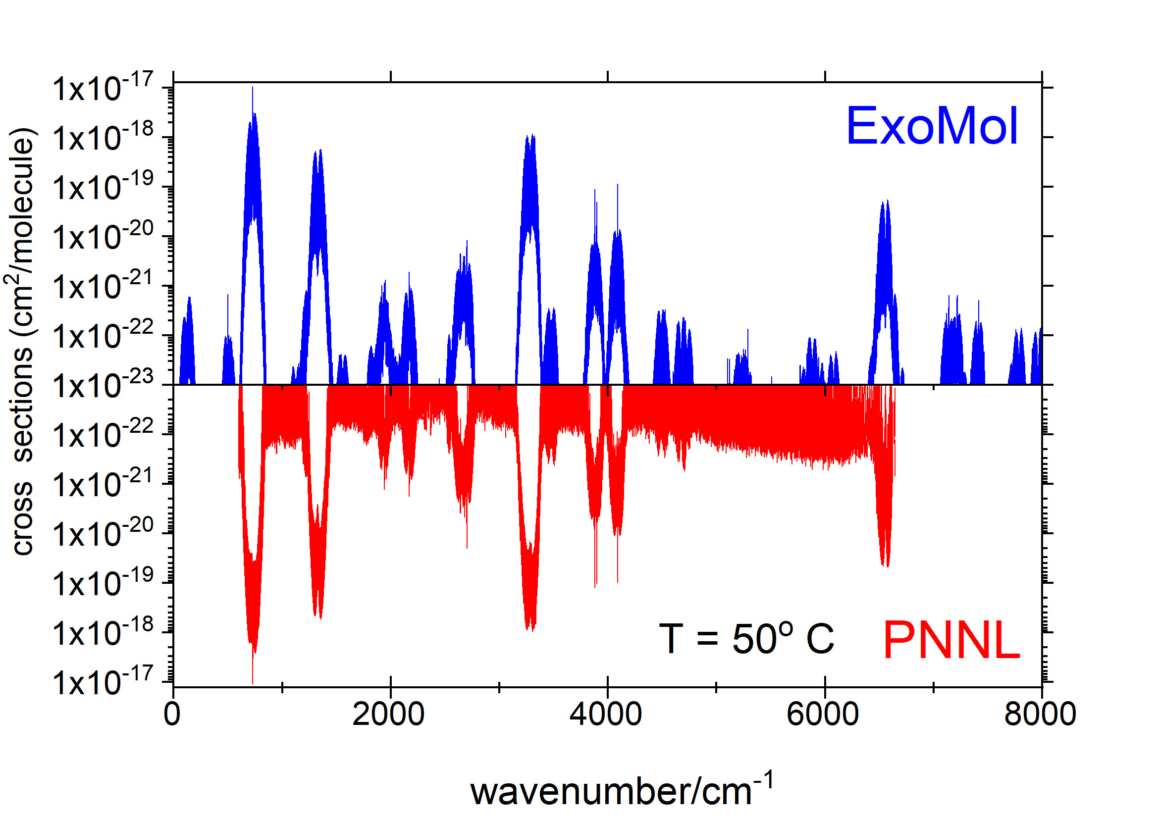
Figure 11: Comparison of the aCeTY cross-sections against PNNL (Sharpe et al., 2004) at $T=$ 50^∘. The aCeTY cross-sections were generated using the Gaussian line profile with half-width-at-half-maximum of $0.01$ cm^-1. The PNNL data below $1\times 10^{-22}$ cm² / molecule are largely due to noise.

5 Exoplanet Atmospheres

Figure 12 gives the transmission spectra of a hypothetical planetary atmosphere of a Jupiter-size planet around a solar-like star, with an atmosphere of pure ¹²C₂H₂, at 1000 K, computed using TauREx (Waldmann et al., 2015). A comparison of such an atmosphere using the aCeTY line list is made against one using HITRAN cross-section data (both are computed at a resolving power of R=${\lambda}/{\Delta\lambda}=$10 000). It can be seen that a large amount of opacity would be lost if one used HITRAN data at high-temperatures. This is further demonstrated by an atmosphere of a planet with the same mass and temperature, which contains H₂O (Polyansky et al., 2018), CO₂ (Rothman et al., 2010a), CH₄ (Yurchenko et al., 2017b), CO (Li et al., 2015), HCN (Barber et al., 2014), H₂S (Azzam et al., 2016) and C₂H₂ at approximately equilibrium abundances. Figure 13 shows the differences between using aCeTY and HITRAN data as input into the transmission spectrum computation for C₂H₂. Low resolution (R=${\lambda}/{\Delta\lambda}=$300) k-tables are used here. All other molecules and parameters remain the same between the two spectra. The cross-sections and k-tables (the latter are produced using a method of opacity sampling which enables low resolution computations while still taking strong opacity fluctuations at high resolution into account; see, for example, Min (2017)) used in these model will shortly be made publicly available (Chubb et al., 2019).

Figure 12: The transmission spectra of a hypothetical planetary atmosphere of a Jupiter-size planet around a solar-like star, with an atmosphere of pure ¹²C₂H₂, at 1000 K, computed using TauREx (Waldmann et al., 2015). A comparison is made using aCeTY (this work) against HITRAN line list data as input into the cross-sections used in the transmission spectrum computation.

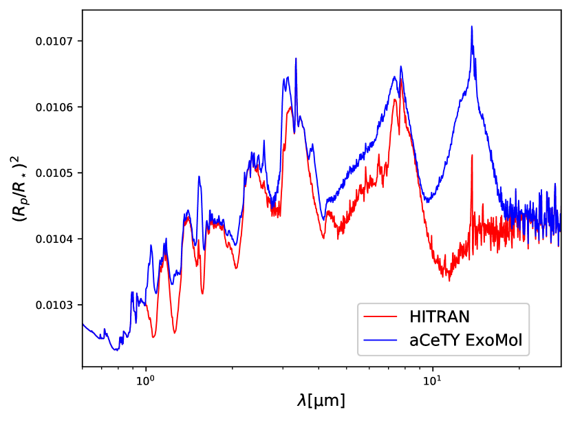
Figure 13: The transmission spectra of a hypothetical planetary atmosphere of a Jupiter-size planet around a solar-like star, with an atmosphere of H₂O, CO₂, CH₄, CO, HCN, H₂S and C₂H₂ at approximately equilibrium abundances at 1000 K, computed using TauREx (Waldmann et al., 2015). A comparison is made using aCeTY (this work) against HITRAN line list data as input into the transmission spectrum computation for C₂H₂. All other molecules and parameters remain the same between the two spectra.

6 Summary and Future Work

In this work we present a new ro-vibrational line list for the ground electronic state of the main isotopologue of acetylene, ¹²C₂H₂; the aCeTY line list. This line list was computed as part of the ExoMol project (Tennyson & Yurchenko, 2012; Tennyson et al., 2016), for characterising exoplanet and cool stellar atmospheres. It is considered complete up to 2200 K, with transitions computed up to 10 000 cm^-1  (down to 1 $\mu$m), with lower and upper energy levels up to 12 000 cm^-1 and 22 000 cm^-1 considered, respectively. The calculations were performed up to a maximum value for the vibrational angular momentum, $K_{\rm max}=L_{\rm max}$ = 16, and maximum rotational angular momentum, $J$ = 99. The aCeTY line list is based on ab initio electronic structure calculations for the potential energy and dipole moment surfaces, but with improvements on the accuracy of both the line positions and the dipole moments made using the wealth of experimental data available from the literature.

Comparisons against other available line list data demonstrate that the aCeTY line list is the most complete and accurate available line list for acetylene to date. It is therefore recommended for use in characterising exoplanet and cool stellar atmospheres. Computing cross-section and k-table opacity data for ¹²C₂H₂, at a range of temperatures and pressures suitable for use in exoplanet atmospheres, for use in retrieval codes such as Tau-REx (Waldmann et al., 2015), ARCiS (Min et al., 2019), NEMESIS (Irwin et al., 2008) and petitRADTRANS (Molliére, P. et al., 2019) will be published in soon (Chubb et al., 2019).

For high-resolution applications, however, some caution is advised. More work needs to be done, which is ongoing, to further improve and ensure the accuracy of line position to achieve precision required for studies of exoplanets using high resolution Doppler spectroscopy. The line list can be improved by augmenting the Marvel analysis of Chubb et al. (2018c) with new laboratory data, such as Twagirayezu et al. (2018); Di Sarno et al. (2019); Nürnberg et al. (2019), and then inserting the resulting energy levels in aCeTY; this would ensure that energies and associated transition wavenumbers are at the current limit of accuracy. The high-accuracy experiments of Tao et al. (2018) and Liu et al. (2013) (which was not included in Chubb et al. (2018c)) demonstrates that updates should be made to the $\nu_{1}+3\nu_{3}$ band included in the Marvel analysis of ¹²C₂H₂.

The new intensity scaling technique presented in this work will be useful for future high-precision spectroscopic applications, especially if combined with the MARVELisation procedure. It has the potential to target the accuracy of experiment when predicting line intensities within a given vibrational band at different temperatures.

The line lists aCeTY can be downloaded from the CDS, via ftp://cdsarc.u-strasbg.fr/pub/cats/J/MNRAS/, or http://cdsarc.u-strasbg.fr/viz-bin/qcat?J/MNRAS/, or from www.exomol.com.

References

- Al-Refaie et al. (2016) Al-Refaie A. F., Polyansky O. L., Ovsyannikov R. I., Tennyson J., Yurchenko S. N., 2016, Mon. Not. R. Astron. Soc., 461, 1012
- Amyay et al. (2009) Amyay B., et al., 2009, J. Chem. Phys., 131, 114301
- Amyay et al. (2016) Amyay B., Fayt A., Herman M., Auwera J. V., 2016, J. Phys. Chem. Ref. Data, 45, 023103
- Aringer et al. (2009) Aringer B., Girardi L., Nowotny W., Marigo P., Lederer M. T., 2009, Astron. Astrophys., 503, 913
- Azzam et al. (2016) Azzam A. A. A., Yurchenko S. N., Tennyson J., Naumenko O. V., 2016, Mon. Not. R. Astron. Soc., 460, 4063
- Ba et al. (2013) Ba Y. A., et al., 2013, J. Quant. Spectrosc. Radiat. Transf., 130, 62
- Bains (2004) Bains W., 2004, Astrobiology, 4, 137
- Barber et al. (2014) Barber R. J., Strange J. K., Hill C., Polyansky O. L., Mellau G. C., Yurchenko S. N., Tennyson J., 2014, Mon. Not. R. Astron. Soc., 437, 1828
- Belay & Daniels (1987) Belay N., Daniels L., 1987, Appl Environ Microbiol., 53, 1604
- Bilger et al. (2013) Bilger C., Rimmer P., Helling C., 2013, Mon. Not. R. Astron. Soc., 435, 1888
- Brogi et al. (2017) Brogi M., Line M., Bean J., Désert J.-M., Schwarz H., 2017, Astrophys. J. Lett., 839, L2
- Brooke et al. (1996) Brooke T. Y., Tokunaga A. T., Weaver H. A., Crovisier J., BockeleeMorvan D., Crisp D., 1996, Nature, 383, 606
- Bunker & Jensen (2006) Bunker P. R., Jensen P., 2006, Molecular Symmetry and Spectroscopy, Second Edition. NRC Research Press, Ottawa, Canada
- Cassady et al. (2018) Cassady S. J., Peng W. Y., Hanson R. K., 2018, J. Quant. Spectrosc. Radiat. Transf., 221, 172
- Cernicharo (2004) Cernicharo J., 2004, Astrophys. J., 608, L41
- Chubb (2018) Chubb K. L., 2018, PhD thesis, University College London, London, UK
- Chubb et al. (2018a) Chubb K. L., Jensen P., Yurchenko S. N., 2018a, Symmetry, 10, 137
- Chubb et al. (2018b) Chubb K. L., Yachmenev A., Tennyson J., Yurchenko S. N., 2018b, J. Chem. Phys., 149, 014101
- Chubb et al. (2018c) Chubb K. L., et al., 2018c, J. Quant. Spectrosc. Radiat. Transf., 204, 42
- Chubb et al. (2019) Chubb K. L., et al., 2019, Astron. Astrophys.
- Coles et al. (2019) Coles P. A., Yurchenko S. N., Tennyson J., 2019, Mon. Not. R. Astron. Soc., 490, 4638
- Cooley (1961) Cooley J. W., 1961, Math. Comp., 15, 363
- Dhanoa & Rawlings (2014) Dhanoa H., Rawlings J. M. C., 2014, Mon. Not. R. Astron. Soc., 440, 1786
- Di Sarno et al. (2019) Di Sarno V., et al., 2019, OPTICA, 6, 436
- Didriche & Herman (2010) Didriche K., Herman M., 2010, Chem. Phys. Lett., 496, 1
- Dinelli et al. (2019) Dinelli B. M., et al., 2019, Icarus, 331, 83
- Drossart et al. (1986) Drossart P., Bézard B., Atreya S., Lacy J., Serabyn E., Tokunaga A., Encrenaz T., 1986, Icarus, 66, 610
- Encrenaz et al. (1986) Encrenaz T., Combes M., Atreya S. K., Romani P. N., Fricke K., 1986, Astron. Astrophys., 162, 317
- Endres et al. (2016) Endres C. P., Schlemmer S., Schilke P., Stutzki J., Müller H. S. P., 2016, J. Mol. Spectrosc., 327, 95
- Furtenbacher et al. (2007) Furtenbacher T., Császár A. G., Tennyson J., 2007, J. Mol. Spectrosc., 245, 115
- Gamache et al. (2017) Gamache R. R., et al., 2017, J. Quant. Spectrosc. Radiat. Transf., 203, 70
- Gaudi et al. (2017) Gaudi B. S., et al., 2017, Nature, 546, 514+
- Gautschy-Loidl et al. (2004) Gautschy-Loidl R., Høfner S., Jorgensen U., Hron J., 2004, Astron. Astrophys., 422, 289
- Gaydon (2012) Gaydon A., 2012, The spectroscopy of flames. Springer Science Business Media B.V. 1974, doi:10.1007/978-94-009-5720-6
- Goebel et al. (1978) Goebel J. H., Bregman J. D., Strecker D. W., Witteborn F. C., Erickson E. F., 1978, Astrophys. J. Lett., 222, L129
- Gordon et al. (2017) Gordon I. E., et al., 2017, J. Quant. Spectrosc. Radiat. Transf., 203, 3
- Herman (2007) Herman M., 2007, Mol. Phys., 105, 2217
- Herman (2011) Herman M., 2011, High-resolution infrared spectroscopy of acetylene: Theoretical background and research trends. John Wiley & Sons, Ltd, pp 1993–2026, doi:10.1002/9780470749593.hrs101
- Hörst (2017) Hörst S. M., 2017, J. Geophys. Res.: Planets, 122, 432
- Hughes & Gorden (1959) Hughes E. E., Gorden R., 1959, Analytical Chemistry, 31, 94
- Irwin (1981) Irwin A.-W., 1981, Astrophys. J. Suppl., 45, 621
- Irwin et al. (2008) Irwin P. G. J., et al., 2008, J. Quant. Spectrosc. Radiat. Transf., 109, 1136
- Jacquemart et al. (2017) Jacquemart D., Lyulin O. M., Perevalov V. I., 2017, J. Quant. Spectrosc. Radiat. Transf., 203, 440
- Jacquinet-Husson et al. (2016) Jacquinet-Husson N., et al., 2016, J. Mol. Spectrosc., 327, 31
- Jørgensen et al. (2000) Jørgensen U. G., Hron J., Loidl R., 2000, Astron. Astrophys., 356, 253
- Kelly et al. (2012) Kelly M. W., Richley J. C., Western C. M., Ashfold M. N. R., Mankelevich Y. A., 2012, J. Phys. Chem. A, 116, 9431
- Lahuis et al. (2005) Lahuis F., et al., 2005, Astrophys. J., 636, L145
- Le Roy et al. (2015) Le Roy L., et al., 2015, Astron. Astrophys., 583, A1
- Lederer, M. T. & Aringer, B. (2009) Lederer, M. T. Aringer, B. 2009, Astron. Astrophys., 494, 403
- Li et al. (2015) Li G., Gordon I. E., Rothman L. S., Tan Y., Hu S.-M., Kassi S., Campargue A., Medvedev E. S., 2015, Astrophys. J. Suppl., 216, 15
- Liu et al. (2013) Liu A.-W., Li X.-F., Wang J., Lu Y., Cheng C.-F., Sun Y. R., Hu S.-M., 2013, J. Chem. Phys., 138, 014312
- Loidl et al. (1999) Loidl R., Høfner S., Jørgensen U. G., Aringer B., 1999, Astron. Astrophys., 342, 531
- Lovett (2011) Lovett R. A., 2011, Enceladus named sweetest spot for alien life, doi:10.1038/news.2011.337
- Lyulin & Campargue (2017) Lyulin O. M., Campargue A., 2017, J. Quant. Spectrosc. Radiat. Transf., 203, 461
- Lyulin & Campargue (2018) Lyulin O., Campargue A., 2018, J. Quant. Spectrosc. Radiat. Transf., 215, 51
- Lyulin & Perevalov (2017) Lyulin O. M., Perevalov V. I., 2017, J. Quant. Spectrosc. Radiat. Transf., 201, 94
- Lyulin et al. (2018) Lyulin O. M., Béguier S., Hu S. M., Campargue A., 2018, J. Quant. Spectrosc. Radiat. Transf., 208, 179
- Lyulin et al. (2019) Lyulin O., Vasilchenko S., Mondelain D., Campargue A., 2019, J. Quant. Spectrosc. Radiat. Transf., 234, 147
- Madhusudhan et al. (2016) Madhusudhan N., Agundez M., Moses J. I., Hu Y., 2016, Space Sci. Rev., 205, 285
- Mant et al. (2018) Mant B. P., Yachmenev A., Tennyson J., Yurchenko S. N., 2018, Mon. Not. R. Astron. Soc., 478, 3220
- Marigo, P. & Aringer, B. (2009) Marigo, P. Aringer, B. 2009, Astron. Astrophys., 508, 1539
- Matsuura et al. (2006) Matsuura M., et al., 2006, Mon. Not. R. Astron. Soc., 371, 415
- McKay & Smith (2005) McKay C. P., Smith H. D., 2005, Icarus, 178, 274
- McKemmish et al. (2016) McKemmish L. K., Yurchenko S. N., Tennyson J., 2016, Mon. Not. R. Astron. Soc., 463, 771
- Metsälä et al. (2010) Metsälä M., Schmidt F. M., Skytta M., Vaittinen O., Halonen L., 2010, J. Breath Res., 4, 046003
- Mikhailenko et al. (2005) Mikhailenko S. N., Babikov Y. L., F. G. V., 2005, Atmospheric and Oceanic Optics, 18, 685
- Miller et al. (2014) Miller L. G., Baesman S. M., Oremland R. S., 2014, AGU Fall Meeting Abstracts, pp P53B–4009
- Min (2017) Min M., 2017, Astron. Astrophys., 607, A9
- Min et al. (2019) Min M., Ormel C. W., Chubb K. L., Helling C., Kawashima Y., 2019, A&A
- Molliére, P. et al. (2019) Molliére, P. Wardenier, J. P. van Boekel, R. Henning, Th. Molaverdikhani, K. Snellen, I. A. G. 2019, A&A, 627, A67
- Moses et al. (2000) Moses J. I., Bézard B., Lellouch E., Gladstone G., Feuchtgruber H., Allen M., 2000, Icarus, 143, 244
- Noumerov (1924) Noumerov B. V., 1924, Mon. Not. R. Astron. Soc., 84, 592
- Nürnberg et al. (2019) Nürnberg J., Alfieri C. G. E., Chen Z., Waldburger D., Picqué N., Keller U., 2019, Opt. Express, 27, 3190
- Oppenheimer et al. (2013) Oppenheimer B. R., et al., 2013, Astrophys. J., 768, 24
- Oremland & Voytek (2008) Oremland R. S., Voytek M. A., 2008, Astrobiology, 8, 45
- Owens et al. (2017) Owens A., Yurchenko S. N., Yachmenev A., Thiel W., Tennyson J., 2017, Mon. Not. R. Astron. Soc., 471, 5025
- Peterson et al. (2008) Peterson K. A., Adler T. B., Werner H.-J., 2008, J. Chem. Phys., 128, 084102
- Polyansky et al. (2017) Polyansky O. L., Kyuberis A. A., Lodi L., Tennyson J., Ovsyannikov R. I., Zobov N., 2017, Mon. Not. R. Astron. Soc., 466, 1363
- Polyansky et al. (2018) Polyansky O. L., Kyuberis A. A., Zobov N. F., Tennyson J., Yurchenko S. N., Lodi L., 2018, Mon. Not. R. Astron. Soc., 480, 2597
- Rangwala et al. (2018) Rangwala N., et al., 2018, Astrophys. J., 856, 9
- Rey et al. (2016) Rey M., Nikitin A. V., Babikov Y. L., Tyuterev V. G., 2016, J. Mol. Spectrosc., 327, 138
- Ridgway (1974) Ridgway S. T., 1974, Astrophys. J., 187, L41
- Ridgway et al. (1976) Ridgway S. T., Hall D. N. B., Kleinmann S. G., Weinberger D. A., Wojslaw R. S., 1976, Nature, 264, 345
- Rinsland et al. (1982) Rinsland C. P., Baldacci A., Rao K. N., 1982, Astrophys. J. Suppl., 49, 487
- Rothman et al. (2010a) Rothman L. S., et al., 2010a, J. Quant. Spectrosc. Radiat. Transf., 111, 2139
- Rothman et al. (2010b) Rothman L., et al., 2010b, J. Quant. Spectrosc. Radiat. Transf., 111, 2139
- Schmidt et al. (2010) Schmidt F. M., Vaittinen O., Metsälä M., Kraus P., Halonen L., 2010, Appl. Phys. B-Lasers Opt., 101, 671
- Seager et al. (2013) Seager S., Bains W., Hu R., 2013, Astrophys. J., 775, 104
- Shabram et al. (2011) Shabram M., Fortney J. J., Greene T. P., Freedman R. S., 2011, Astrophys. J., 727, 65
- Sharpe et al. (2004) Sharpe S. W., Johnson T. J., Sams R. L., Chu P. M., Rhoderick G. C., Johnson P. A., 2004, Appl. Spectrosc., 58, 1452
- Singh et al. (2016) Singh S., et al., 2016, Astrophys. J., 828, 55
- Sousa-Silva et al. (2015) Sousa-Silva C., Al-Refaie A. F., Tennyson J., Yurchenko S. N., 2015, Mon. Not. R. Astron. Soc., 446, 2337
- Tanaka et al. (2007) Tanaka M., Letip A., Nishimaki Y., Yamamuro T., Motohara K., Miyata T., Aoki W., 2007, Publications of the Astronomical Society of Japan, 59, 939
- Tao et al. (2018) Tao L.-G., Hua T.-P., Sun Y. R., Wang J., Liu A.-W., Hu S.-M., 2018, J. Quant. Spectrosc. Radiat. Transf., 210, 111
- Tennyson & Yurchenko (2012) Tennyson J., Yurchenko S. N., 2012, Mon. Not. R. Astron. Soc., 425, 21
- Tennyson & Yurchenko (2016) Tennyson J., Yurchenko S., 2016, Exp. Astron., 40, 563
- Tennyson & Yurchenko (2017) Tennyson J., Yurchenko S. N., 2017, Mol. Astrophys., 8, 1
- Tennyson et al. (2013) Tennyson J., Hill C., Yurchenko S. N., 2013, in 6th international conference on atomic and molecular data and their applications ICAMDATA-2012. AIP, New York, pp 186–195, doi:10.1063/1.4815853
- Tennyson et al. (2016) Tennyson J., et al., 2016, J. Mol. Spectrosc., 327, 73
- Tsiaras et al. (2016) Tsiaras A., et al., 2016, Astrophys. J., 820, 99
- Tsuji (1986) Tsuji T., 1986, Annual review of astronomy and astrophysics, 24, 89
- Twagirayezu et al. (2018) Twagirayezu S., Hall G. E., Sears T. J., 2018, J. Chem. Phys., 149, 154308
- Underwood et al. (2016a) Underwood D. S., Tennyson J., Yurchenko S. N., Huang X., Schwenke D. W., Lee T. J., Clausen S., Fateev A., 2016a, Mon. Not. R. Astron. Soc., 459, 3890
- Underwood et al. (2016b) Underwood D. S., Tennyson J., Yurchenko S. N., Clausen S., Fateev A., 2016b, Mon. Not. R. Astron. Soc., 462, 4300
- Waite et al. (2006) Waite J. H., et al., 2006, Science, 311, 1419
- Waldmann et al. (2015) Waldmann I. P., Tinetti G., Rocchetto M., Barton E. J., Yurchenko S. N., Tennyson J., 2015, Astrophys. J., 802, 107
- Watson (1968) Watson J. K. G., 1968, Mol. Phys., 15, 479
- Werner et al. (2012) Werner H.-J., Knowles P. J., Knizia G., Manby F. R., Schütz M., 2012, WIREs Comput. Mol. Sci., 2, 242
- Yachmenev & Yurchenko (2015) Yachmenev A., Yurchenko S. N., 2015, J. Chem. Phys., 143, 014105
- Yurchenko & Tennyson (2014) Yurchenko S. N., Tennyson J., 2014, Mon. Not. R. Astron. Soc., 440, 1649
- Yurchenko et al. (2003) Yurchenko S. N., Carvajal M., Jensen P., Herregodts F., Huet T. R., 2003, Chem. Phys., 290, 59
- Yurchenko et al. (2007) Yurchenko S. N., Thiel W., Jensen P., 2007, J. Mol. Spectrosc., 245, 126
- Yurchenko et al. (2011a) Yurchenko S. N., Barber R. J., Tennyson J., Thiel W., Jensen P., 2011a, J. Mol. Spectrosc., 268, 123
- Yurchenko et al. (2011b) Yurchenko S. N., Barber R. J., Tennyson J., 2011b, Mon. Not. R. Astron. Soc., 413, 1828
- Yurchenko et al. (2014) Yurchenko S. N., Tennyson J., Bailey J., Hollis M. D. J., Tinetti G., 2014, Proc. Nat. Acad. Sci., 111, 9379
- Yurchenko et al. (2017a) Yurchenko S. N., Yachmenev A., Ovsyannikov R. I., 2017a, J. Chem. Theory Comput., 13, 4368
- Yurchenko et al. (2017b) Yurchenko S. N., Amundsen D. S., Tennyson J., Waldmann I. P., 2017b, Astron. Astrophys., 605, A95
- Yurchenko et al. (2018) Yurchenko S. N., Al-Refaie A. F., Tennyson J., 2018, Astron. Astrophys., 614, A131
- Zak et al. (2017) Zak E. J., Tennyson J., Polyansky O. L., Lodi L., Zobov N. F., Tashkun S. A., Perevalov V. I., 2017, J. Quant. Spectrosc. Radiat. Transf., 189, 267
- de Graauw et al. (1997) de Graauw T., et al., 1997, Astron. Astrophys., 321, L13
- de Kok et al. (2014) de Kok R. J., Birkby J., Brogi M., Schwarz H., Albrecht S., de Mooij E. J. W., Snellen I. A. G., 2014, Astron. Astrophys., 561, A150
- van Dishoeck et al. (1998) van Dishoeck E. F., Wright C. M., Cernicharo J., González-Alfonso E., de Graauw T., Helmich F. P., Vandenbussche B., 1998, The Astrophysical Journal, 502, L173